Download - GCOE Discussion Paper Series - Osaka U
Discussion Paper No. 171
Weather and Individual Happiness
Yoshiro Tsutsui
January 2011; revised March 2012
GCOE Secretariat Graduate School of Economics
OSAKA UNIVERSITY 1-7 Machikaneyama, Toyonaka, Osaka, 560-0043, Japan
GCOE Discussion Paper Series
Global COE Program Human Behavior and Socioeconomic Dynamics

Weather and Individual Happiness
Yoshiro Tsutsui
Osaka University
Abstract
This paper investigates the influence of weather on happiness. While previous studies
have examined climatic influence by comparing the well-being of people living in
different regions, this paper focuses on how daily changes in weather affect individuals
living in a single location. Our data set consists of 516 days of data on 75 students from
Osaka University. Daily information on outside events, as well as the daily physical
condition and individual characteristics of the respondents, are used as controls.
Subjective happiness is negatively related to temperature and humidity. In a quadratic
model, happiness is maximized at 13.9 degrees Celsius. The effects of other
meteorological variables—wind speed and precipitation—are not significant. The
sensitivity of happiness to temperature also depends on attributes such as sex, age, and
academic department. Happiness is more strongly affected by current weather
conditions than average weather over the day. While sadness and depression (negative
affect) are affected by weather in a similar way to happiness, enjoyment (positive affect)
behaves somewhat differently.
JEL Classification Number: I31, Q51, Q54
Keywords: happiness, weather, daily web survey, Osaka region
Correspondence to: Graduate School of Economics, Osaka University 1-7 Machikane-yama, Toyonaka, 560-0043 Japan Phone: +81-6-6850-5223 Fax: +81-6-6850-5274 E-mail: [email protected]
Running title : Weather and Individual Happines I am grateful for the insightful comments by two anonymous reviewers of this journal, which triggered a revision and extension of the earlier version. Financial support from the 21st Century Center of Excellence (COE) and Global Center of Excellence (GCOE) programs of Osaka University is gratefully acknowledged.
- 1 -
1. Introduction
This paper seeks to identify the effect of weather on happiness. Although economists are
interested in the material factors shaping happiness, such as income (Frey and Stutzer 2002),
happiness is known to depend on a broader range of variables, including education, health, and
personal characteristics such as age, gender, ethnicity, and personality (Dolan et al. 2008).
Climate and the natural environment also affect happiness.1 There have been many
studies arguing that climate is an important element of quality of life (e.g. see Moro et al. 2008,
Oswald and Wu 2010).2 In spite of the importance of climate, a relatively limited number of
studies have analyzed its influence on happiness (Dolan et al. 2008).3
A survey of earlier studies on the impact of climate on happiness indicates the current
state of this field of inquiry. Rehdanz and Maddison (2005) analyzed a panel of 67 countries and
found that temperature and precipitation have a significant effect on happiness. Specifically,
people prefer higher mean temperatures in the coldest month and lower temperatures in the
1 Recall the famous lyric by the Carpenters: “Rainy days and Mondays always get me down.” 2 Additional direct evidence for the fact that people regard a pleasant climate as essential for a good life and for personal satisfaction is obtained from a large-scale survey conducted by Osaka University in 2007 and 2008. In that survey, respondents were asked to select a prefecture in which they wished to live and to select the reasons for their choices. Of the 16 possible reasons, "Nice climate and rich natural environment” was tied for the most common. 3 Several articles analyze the effect of climate on life patterns. For example, Maddison (2003) demonstrated that climate is a significant determinant of expenditure patterns. Hoch and Drake (1974) investigated the relation between climate and wages, under the hypothesis that higher money wages compensate for a lower quality of life. Maddison and Bigano (2003) studied the relationship between climate and wage and home price differentials in Italy. Van Praag (1988) researched the dependence of household costs on climatic conditions, and estimated a climate index and climate equivalence scales for European cities. Bigano et al. (2008) analyzed the effect of climate on sea levels and tourism flows.
- 2 -
hottest month. Those living in regions with many dry months prefer more precipitation.
Examining the data on Ireland, Brereton et al. (2008) found that wind speed has a significant
negative influence on happiness, while the effects of increases in both January minimum and
July maximum temperatures are positive and significant. Using the first two waves of the
Russian National Panel data set on 3,727 households in 1993 and 1994, Frijters and van Praag
(1998) revealed that while temperature and precipitation exert a measurable influence on
self-reported happiness and on the cost of living in Russia, the effects of climate in that nation
are different from those in the rest of Europe, an incongruity that “is probably due to the greater
range of climate in Russia.”
Psychologists have studied the relationship between mood and weather. Recently, using
three large-scale German surveys, Kämpfer and Mutz (2011) found that respondents surveyed
on days with exceptionally sunny weather reported higher life satisfaction compared with
respondents interviewed on days with “ordinary” weather. Using data from a large-scale
depression-screening program in the south of the Netherlands, Huibers et al. (2010) reported
that the prevalence of major depression and sad mood showed seasonal variation, with peaks in
the summer and fall. Eisinga et al. (2011) found that television viewing time in the Netherlands
is related to weather.
Most of these previous studies have examined the effect of climate by comparing the
- 3 -
happiness of the residents of different regions or countries. Although the studies conclude that
happiness is affected by regional differences in climate, they are unable to assess whether the
happiness of an individual responds to daily weather variations. Answering the latter question
requires time series data on individual happiness rather than cross-sectional data. Thus, the
central question in this study - whether the happiness of individuals varies with daily weather
changes – has not yet been definitively answered.
One notable exception is Schwarz and Clore (1983), who telephoned 84 German subjects
on sunny and rainy days to ask about their immediate mood (momentary happiness) and
well-being (general life happiness). On sunny days subjects reported higher levels of
momentary happiness, while on rainy days mood was lower. This study suggests that
momentary happiness depends on current weather. Barnston (1988), using six-week
mood/productivity diaries from 62 students in 1974, report that the weather appears to influence
mood and productivity, but only to a small extent.
Recently, three more relevant studies have been published. Denissen et al. (2008)
collected mood data for 1,233 people over 14 days, and found that temperature, wind power,
and sunlight influence negative affect. However, the size of the effect of weather on mood was
small. Kööt et al. (2011), sampling subjects’ affect for 14 days on 7 occasions per day, found
that positive and negative affect were weakly related to temperature, and that positive affect was
- 4 -
also related to sunlight. Klimstra et al. (2011) identified weather reactivity types by linking
self-reported daily mood across 30 days to objective weather data. They found large individual
differences in how people’s moods were affected by weather, which may hide the effect of
weather on mood as a whole.
A limitation of these studies is the limited number of sampling days: even the longest
study covers only six weeks. In order to investigate the effect of weather on happiness or mood,
it is desirable to analyze data covering the whole year.
To this end, I conducted a daily web survey to collect data on the levels of happiness of
75 college students over 17 months, resulting in 32,125 observations. Additionally, I collected
daily data on important individual-level control variables. Though many studies have concluded
that the effect of weather is weak (if it exists at all), controlling for individual factors that are
likely to affect happiness (or mood) may increase weather’s effect size. In this paper, daily
information on events that occurred on the same day, and on the physical conditions of the
respondents, are used as control variables (in addition to fixed individual characteristics, or
“attributes”).
The rest of this paper is organized as follows: In Section 2, I explain the data and methods.
The subsequent section presents the basic estimation results. In Section 4, I check the robustness
of the results, and extend the basic equation to incorporate individual attributes. Section 5
- 5 -
concludes.
2. Data and Methods
2.1 The daily web survey
Survey participants consisted of 70 undergraduate and graduate students of Osaka University.
We asked these respondents to report their daily happiness and their evaluation of the day’s
personal events and news. The survey was conducted from November 1, 2006 to March 31,
2008. Since five subjects did not finish the survey, I added five more subjects in the middle of
the survey period, increasing the total number of respondents to 75. At the outset of the web
survey, detailed data on the attributes (fixed individual characteristics) of each subject were
collected.
Subjects were paid 160 yen per daily survey response. Additionally, those who responded
more than 22 days in a month were paid 1300 yen as a bonus, while those who answered more
than 27 days received 2600 yen.4 The overall daily response rate was about 89%.
The first question in the daily web survey was: “(Q1) How happy are you now?” The
respondents answered this question on a scale of 0 to 10, where 0 was “very unhappy” and 10
4 Respondents were also asked to report their happiness every hour over one day of their choice per month. Answering this hourly survey was a necessary condition for the monthly bonus.
- 6 -
was “very happy.” I named this variable HAPPINESS.5
Other questions also attempted to assess subjects’ emotional state. Question 5 asked:
“What was the most important piece of personal news that you received since responding to the
questionnaire yesterday? How do you evaluate this news?” The answer, labeled P_NEWS,
could range between -5 and 5, where 5 was “very good” and -5 was “very bad.” Question 7
asked about news received via public news media: “What was the most important piece of
news from television or newspapers that you received since responding to the questionnaire
yesterday? How do you evaluate this news?” This answer, labeled M_NEWS (for “macro
news”), could also range between -5 and 5.
Some questions asked respondents about their physical condition, which I named SLEEP,
HEALTH, and STRESS. SLEEP was defined as the answer to the following question: “(Q9) Did
you sleep well last night?” An answer of 1 indicated poor sleep; 2, somewhat poor sleep; 3,
good sleep; and 4, very good sleep. HEALTH was assessed with the following question: “(Q10)
How is your health now?” The answers ranged from 1 (good), 2 (generally good), 3 (generally
not good), to 4 (bad); the variable HEALTH was defined by subtracting the answer to this
question from 5. STRESS was defined by the answer to the following question: “(Q11) Do you
feel any stress now?” Answers ranged from 1 (a lot), 2 (a little), 3 (not much), and 4 (none).
5 In section 4.6, I investigate the effect of weather on affect measures other than self-reported happiness.
- 7 -
Variables were defined so a higher value corresponded to a physical condition presumably more
conducive to happiness (better health, less stress, etc.).
2.2 Meteorological data
Weather data was obtained from the website of the Meteorological Agency of Japan. Hourly and
daily data on temperature (TEMPERATURE), humidity (HUMIDITY), wind speed
(WINDSPEED), precipitation (PRECIPITATION), and hours of sunshine (SUNSHINE) are
available for Osaka city. The hourly data of TEMPERATURE, HUMIDITY, and WINDSPEED
are the values taken at the beginning of the hour, PRECIPITATION is the total precipitation over
the hour, and SUNSHINE is the fraction of sunshine time over the hour. Since the exact time of
each subject’s survey responses was recorded automatically, I matched each individual response
with hourly weather data at the time of the response. However, in order to consider the
possibility that happiness was influenced by the average weather over the entire day rather than
the weather at the time of the survey response, I also included daily averages in the analysis
(subsection 4.5).
Although the exact location of respondents at the time they answered the survey is not
known, they were almost certainly in the Osaka region for most of the time, because all subjects
were students of Osaka University when the survey was conducted. Osaka University has two

- 8 -
campuses, one in Toyonaka and one in Suita, which are suburbs of Osaka (see Figure 1).6 The
distance between the two campuses is only about five kilometers, so that the difference in
weather between the two is not considerable. Weather data for Suita are not available, while
only limited data are available for Toyonaka. One reason to use Toyonaka’s weather data would
be that it is the location of one of the campuses. On the other hand, the Osaka weather data is
richer. Furthermore, the distance between Toyonaka campus and the Osaka City Hall is only 13
kilometers, so that the weather of these two cities does not differ very much. For these reasons I
use the Osaka weather data in my baseline analyses, but I check the robustness of the results
with the Toyonaka data when applicable. I conclude that using the meteorological data of Osaka
city does not produce large biases in any of my estimates (see subsections 4.1 and 4.3).
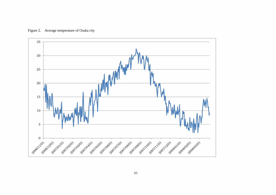
Osaka city is located in the middle of Japan, facing Osaka Bay. The daily average
temperatures for the observation period, which ranged between 5 and 30 degrees Celsius, are
shown in Figure 2. The climate of Osaka is mild and characterized by four seasons, of which
spring and autumn are most loved by residents.7 Winter is not severe: the average temperature
in February, the coldest month, was around 5 degrees Celsius, with almost no snow in the
observation years. However, it is hot and humid in summer; the average temperature in August
was around 30 degrees during the observation period. Osaka residents often complain about the
6 Out of 75 total subjects, 38 belong to Suita campus, 32 to Toyonaka, and five unknown. 7 Sei Shonagon described beautiful scenes set in both of these seasons in her famous book Makurano Soshi (The Pillow Book), written in the 10th and 11th centuries.
- 9 -
high temperature and high humidity of the city in summer. Indeed, the discomfort index (DI)
rises to a high value (80) in August.8 The correlation coefficient between DI and temperature
for the observation period is over 0.99, suggesting that high temperatures made people in Osaka
uncomfortable.
2.3 Descriptive analysis of the data
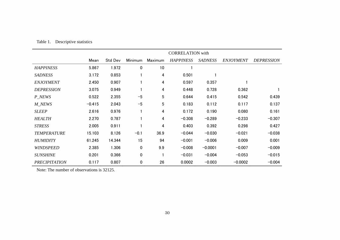
Table 1 presents the means, standard deviations, and maximum and minimum values of the
variables used in this paper, along with the correlation coefficients between HAPPINESS and
the other variables. The observation period is from November 1, 2006 to March 31, 2008, and
the number of observations is 32,125. The means displayed in the table indicate that personal
news is, on average, good (positive), while macro news is generally bad (negative). Average
temperature is about 15 degrees Celsius; average humidity, about 60%; average wind speed, 2.4
m/s; average time of sunshine per hour, about 0.2 hours; and average precipitation per hour,
0.12 mm.
The correlations of P_NEWS, HEALTH, and STRESS with HAPPINESS are quite high.
Among the meteorological variables, TEMPERATURE shows the highest correlation with
happiness, followed by SUNSHINE; however, the size of these correlations is much less than
8 For an explanation of the discomfort index, see Tselepidaki et al. (1992).
- 10 -
that of P_NEWS, suggesting that the effect of weather is relatively limited, if it exists at all.
2.4 Statistical methods
I regress HAPPINESS on the variables representing the conditions of the subjects, the
meteorological variables, and the day-of-the-week dummies.9 Thus, the basic equation to be
estimated is:
, , , , ,
, ∑ , ,
, , , , , , (1)
where is an individual-level fixed effect and , is a disturbance term.
I estimate all the equations with three models: ordinary least squares (OLS), a fixed
effects model, and a random effects model, and then for each regression select a model using a
Hausman test (random effects model vs. fixed effects model) and an F-test of the same constant
(OLS vs. fixed effects model). 10 Section 4 contains several modifications of the basic
regression equation, included as robustness checks.
9 In subsection 4.4, I check whether the results are robust to inclusion of respondent attributes in the regression. 10 Since happiness is an ordered variable, it should be estimated with an ordered probit (logit). However, because it is difficult to interpret the effect sizes in such models, and because controlling for individual-level effects is important, I use the fixed and random effects models.
- 11 -
3. Estimation results of the basic equation
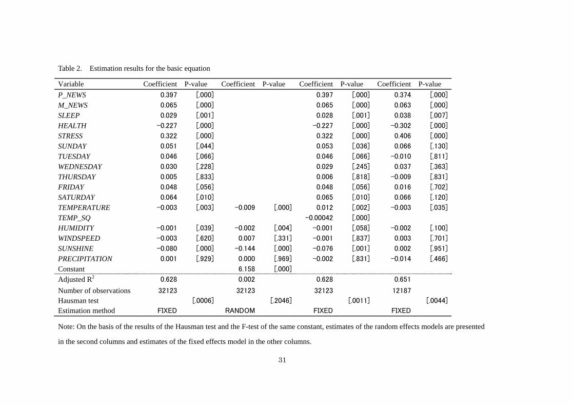
The estimation results are shown in Table 2. In the first column, I show the results for the basic
equation (1).11 All control variables associated with the conditions of the subjects are highly
significant, with reasonable signs. The coefficients on P_NEWS, HEALTH, and STRESS are
especially large, while M_NEWS and SLEEP also have some impact. Estimates for
day-of-the-week dummies reveal that the subjects are significantly happier on Sunday and
Saturday than on Monday. The magnitude of the weekend effect is comparable to that of macro
news.
Among the meteorological variables, temperature, humidity, and sunshine are significant
at the 5% level. The estimated coefficients of temperature and humidity take a negative sign,
implying that the students of Osaka University are happier when the temperature and humidity
are lower. The coefficient on sunshine also takes a negative sign.
In the second column of the table, I present the results when all control variables are
omitted.12 The adjusted R-squared falls from 0.628 to 0.0024, confirming the importance of the
control variables. However, the sign and significance of the estimates of the meteorological
variables does not change much, suggesting that the meteorological variables are not correlated
with the control variables; temperature, humidity, and sunshine are negative and significant at
11 In this case, the fixed effects model was selected. 12 In this case, the random effects model was selected.
- 12 -
the 1% level, while the other variables are not significant.
The finding that subjects liked lower temperatures is consistent with our intuition, since
summer in Osaka is generally perceived to be too hot. However, it does not seem reasonable to
assert that temperature has a linear negative influence, because the temperature in winter is
rather low in the Osaka region. Thus, it is reasonable to assume that there is a temperature
within the observed range that maximizes happiness. To assess this, I add squared temperature
(TEMP_SQ) to the basic specification; the estimation results are shown in the third column of
Table 2. The linear term and the squared term are significantly positive and negative,
respectively, at the 1% level. This result implies that the subjects are the happiest at 13.9
degrees Celsius, which is the average temperature in April and November.
The result that longer sunshine time lowers happiness contradicts our intuition. The
reason of this result may be that SUNSHINE takes a zero value during nighttime, during which
people tend to be happier (Kahneman et al., 2004). To assess this effect, I added hour dummies
for each hour of the day to the basic equation. Subjects were significantly happier from 19:00 to
23:00 than during the daytime. The coefficients on SUNSHINE and HUMIDITY became
insignificant when hour dummies were included, while that on TEMPERATURE remained
significantly negative at the 1% level (results not shown). When hour dummies were added to
the model with no control variables, the coefficient on SUNSHINE became significantly
- 13 -
positive.
In addition, I re-estimated the basic equation while excluding all data reported at night.
Estimates using data from 7:00 to 17:00 are presented in the fourth column of Table 2. The
number of observations was reduced to 12,187. While temperature remained significant at the
5% level, SUNSHINE became insignificant. Given these results, I conclude that the negative
coefficient on SUNSHINE is spurious, and merely reflects the fact that people are happier at
night.
Since some meteorological variables are more correlated with each other than with
HAPPINESS, a multicollinearity problem is suspected. Thus, I re-estimated the model including
only one meteorological variable at a time. The coefficient on humidity became insignificant,
while the other coefficients did not change much (results not shown).
Overall, temperature has the most noteworthy effect among the meteorological variables.
Still, the magnitude of the estimate is not large: the change in happiness brought about by an
alteration of 20 degrees Celsius is equivalent in size to a change in one point of macro news on
a ten-point-scale. This result is consistent with previous studies (Denissen et al. 2008, Barnston
1988).
4. Robustness checks and extensions
- 14 -
In this section, I check the robustness of the results obtained in the previous section and extend
the basic equation in several ways. First, I assess whether the results are valid when I use data
from Toyonaka city instead of Osaka city for some of the meteorological variables. Second, I
separate the total period into “summer” and “winter” seasons and check if the result in the
previous section on temperature is confirmed. Third, since the exact location of respondents is
not known, I examine if lack of this information brings about large biases. Specifically, I utilize
the information on days when the respondents travel and on days when they attend classes to
infer whether subjects stayed near the Toyonaka-Osaka region during the bulk of the
observation period. Fourth, I extend the model to incorporate variables representing the
attributes (fixed individual characteristics) of respondents - sex, age, living standard, body mass
index, etc. I examine not only the effect of these variables on happiness, but also their effects on
the sensitivity of happiness to weather. Fifth, I estimate the basic equation with daily
meteorological data instead of hourly data. Finally, I determine if the meteorological variables
have the same effect on alternative positive and negative affect variables (such as sadness,
pleasure, and depression) that they have on happiness.
4.1 Examination of possible bias due to the use of Osaka city data instead of Toyonaka city
data
- 15 -
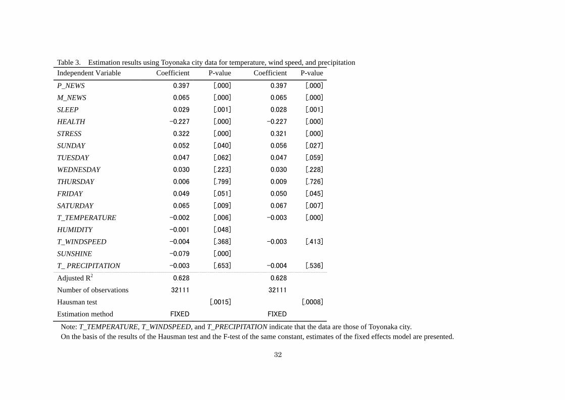
Let me begin with the analysis using the Toyonaka city data. Since one of the two campuses of
Osaka University is in Toyonaka city, it might be the case that subjects spent more time in
Toyonaka city than in Osaka city. Thus, it is interesting to check the size of the biases arising
from the use of Osaka city weather data instead of Toyonaka city data. In a re-estimation of the
basic model, I use Toyonaka data for temperature (T_TEMPRETURE), wind speed
(T_WINDSPEED), and precipitation (T_PRECIPITATION), and Osaka city data for humidity
and sunshine (as these latter two are not available for Toyonaka city). The estimation results are
presented in the left-hand columns of Table 3. The estimates are quite similar to those in Table 2,
implying that using the alternative city data does not affect the results. The right-hand columns
of Table 3 show the results when the data from Osaka city, HUMIDITY and SUNSHINE, are
deleted; the estimates are again quite similar. This is not surprising, since the two cities are quite
near, so that the correlation between the Osaka and Toyonaka data is 0.992 for temperature,
0.495 for wind speed, and 0.389 for precipitation. These results support, at least partially, the
use of the meteorological data of Osaka city, even though respondents’ exact locations are not
known.
4.2 Effect of temperature is opposite in summer and winter
In section 3, it was demonstrated that happiness increases with temperature up to about 14
- 16 -
degrees Celsius, and then decreases. This result leads to the prediction that in summer people
like lower temperatures, while in winter they prefer higher temperatures. To see if this is really
the case I divide the total observation period into two seasons, warm (“summer”) and cold
(“winter”), and re-estimate the basic equation; the former period is from May 16 to November
15, while the latter includes the remainder of the sample period.13
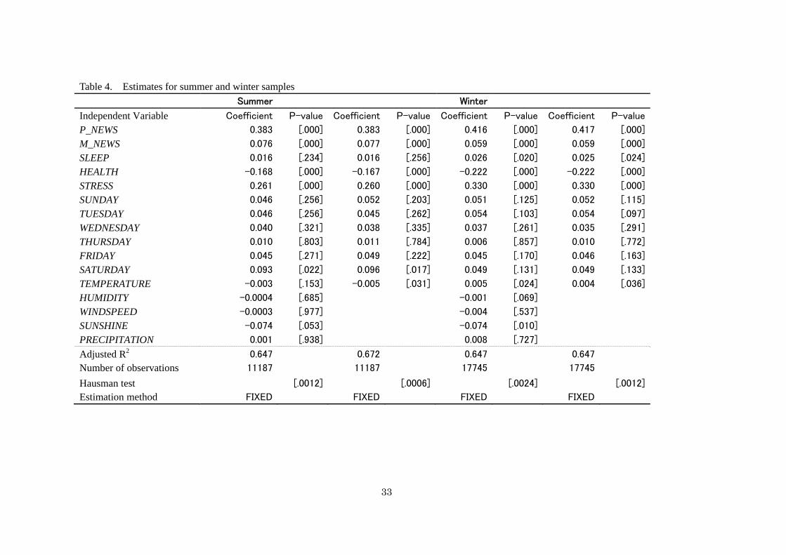
The estimation results are presented in Table 4. In the first columns, the results for
“summer” are shown. Most of the estimates are similar to those in Table 2, confirming the basic
results. However, although the key coefficient of TEMPERATURE takes a negative sign, it is
insignificant at the 10% level. In the second column, I show the estimates when meteorological
variables other than TEMPERATURE are omitted. The coefficient on TEMPERATURE becomes
significantly negative at the 5% level, supporting the prediction. In the table’s third column, the
results for “winter” are presented. The coefficient on TEMPERATURE is significantly positive
at the 5% level, again confirming the prediction. When meteorological variables other than
TEMPERATURE are omitted, the result is unchanged. These results indicate that people in the
Osaka region do not like higher temperatures in summer, but do like them in winter, as one
would expect.14
13 Note that the total period started in “winter” time and ended in “winter” time sixteen months later; thus, the “winter” sample consists of two separated periods, while the “summer” time consists of one consecutive period. 14 I also re-did the estimation dividing the total period into three subperiods: “winter” defined as January to March, “summer” defined as July to September, and “other seasons” (spring and
- 17 -
4.3 Analysis using data on travel and class attendance
One potential problem with the survey data is that the location of respondents at the time of
response is not recorded. However, the respondents are all students of Osaka University, so that
they live within a relatively small region, near the Toyonaka-Suita area, over which hourly
weather is almost uniform. Indeed, in subsection 4.1, I confirmed that the use of Toyonaka or
Osaka city data does not change the results at all. Thus, the use of Osaka data is acceptable and
does not lead to large biases, except on days when respondents traveled away from the area. In
this subsection, I will further examine the robustness of the results, utilizing two additional
location variables that give some indication of respondents’ locations.
In the questionnaire, I asked the respondents to rank the importance of their most
important personal event on that day, and to identify the event. One hundred and forty seven
answers listed travel as the most important event. This is a small number out of the total of
32,125 answers (0.5%). This does not mean that these are all the trips the subjects made over
the sample period, since in most cases they stopped responding to the survey while they were
traveling for a long time, especially when they went abroad. On the other hand, subjects
probably reported their trips when they could, because traveling represents an important
autumn). The coefficient for winter was positive and that for summer was negative, but they were insignificant at the 10% level. The reason for these insignificant results is probably that variation of temperature is small within each season.
- 18 -
personal event. Therefore, it is reasonable to suppose that subjects’ responses were made near
the Osaka region, unless they explicitly noticed that they were traveling.
When I add a cross term between TEMPERATURE and a travel dummy (equal to unity if
a respondent was traveling and zero otherwise) to the basic equation, the coefficient of the cross
dummy is positive (p-value of 23%). Although the significance level is low, the result suggests
that the effect of TEMPERATURE became smaller when subjects made a trip, suggesting that
deleting the traveling samples strengthens the sensitivity of happiness to temperature. In
addition, estimation results when deleting traveling samples produces almost identical results to
those shown in Table 2, suggesting that the results in the previous section are robust (results not
shown). Estimation results for the basic equation using only traveling samples (N=147) are
shown in the left-hand columns of Table 5. While P_NEWS and STRESS are significant and
positive, all meteorological variables, including TEMPERATURE and SUNSHINE, are
insignificant; this is exactly what one would expect, although it may also arise from the small
sample.
From December 1, 2007 to March 31, 2008, I collected data on whether respondents
attended class on the day of the response. The total number of responses during this period is
7,459, while the number during which students attended class is 2,342. It is essentially certain
that students were in the Osaka area when the “attended class” responses were made.
- 19 -
To measure the effect of attending class on happiness and on its sensitivity to temperature,
I added a dummy variable CLASS that takes a value of unity if a subject attended class on the
day of response and zero otherwise, as well as a cross term between TEMPERATURE and the
CLASS dummy (CLASS*TEMP), to the basic equation; the estimation results are presented in
the middle columns of Table 5. The coefficients on the variables of news and physical
conditions are quite similar to those in Table 2. The coefficient on CLASS is negative, but not
significant at the 10% level, suggesting that attending a class might have lowered happiness. As
for the meteorological variables, one notable result is that the coefficient on TEMPERATURE is
positive and significant at the 10% level, suggesting that higher temperature relates to higher
happiness. This is reasonable because the sample period is in the winter season.
Day-of-the-week dummies are not significant here. This is also reasonable, because the period
includes a two-week New Year vacation and term examinations in early February, followed by
one and a half months of spring vacation, so that the distinction between weekdays and
weekends was not very important during the period. The cross term is positive but insignificant,
suggesting that attending class does not affect the sensitivity of happiness to temperature. This
last result has an important implication for the current paper. Reports on days on which subjects
attended a class were definitely sent from Toyonaka-Osaka region. The result that class
attendance does not affect my estimates suggests that subjects also stayed in the
- 20 -
Toyonaka-Osaka region on most of the days when they had no classes. This result is consistent
with the report that subjects made only 147 responses while traveling.
Weekdays and weekends might see different effects on the sensitivity of happiness to
meteorological variables. To assess this, I added a cross term between TEMPERATURE and a
weekend dummy to the basic equation; the estimation results are presented in the right-hand
columns of Table 5. The cross term is not significant at all, indicating that the sensitivity of
happiness to temperature does not differ between weekdays and weekends.
To reiterate, the effect of temperature in Osaka city on happiness when respondents were
traveling is smaller than when they were not. In addition, the sensitivity to temperature does not
differ based whether or not subjects attended class on the day or whether it was a weekday or
weekend. These results suggest that the subjects made most of their answers while in the
Toyonaka-Osaka region, so that biases from day-to-day location changes is very small.
4.4 Effects of attributes on the sensitivity of happiness to temperature
At the start of the web survey in 2006, I sent a paper questionnaire to the respondents to
investigate their attributes (fixed individual characteristics). Thus, it is possible to examine
whether the inclusion of these attributes as regressors changes the estimates of the basic model
from section 3. The variables that I add to the basic model are a dummy variable for male sex
- 21 -
(DMAN), age (AGE), current living standard ranked from 0 to 10 (LIVING), living standard
when subjects were 15 years old (LIVING15), a variable coding the highest education level that
subjects’ fathers finished (F_ACADEMIC, which takes larger values for higher education levels),
an equivalent variable for subjects’ mothers (M_ACADEMIC), smoking habit (SMOKING)
ranging from 1 (do not smoke) to 6 (more than two boxes per day), body mass index (BMI),
strength of religious belief on a five-point scale (RELIGION), and a dummy variable for area of
academic study that takes a value of unity when respondents belong to science departments and
0 when they are affiliated with humanities or social science departments (SCIENCE).
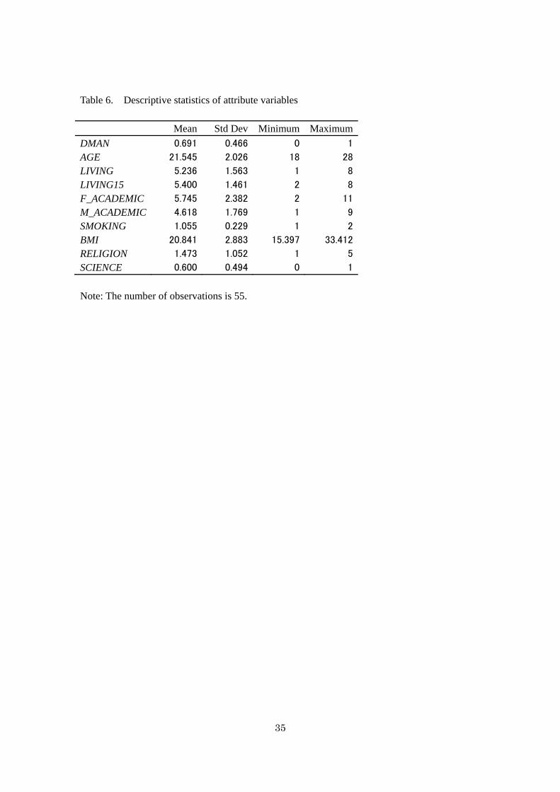
Descriptive statistics for these variables are presented in Table 6. Out of 55 respondents
who answered all the questions, the number of males is 38 (69%). Age ranges from 18 to 28
years old, with an average of 21.5. Only three subjects smoke, and these are all light smokers.
BMI ranges between 15 and 33, with an average of 20.8. Most of the subjects are not deeply
religious.
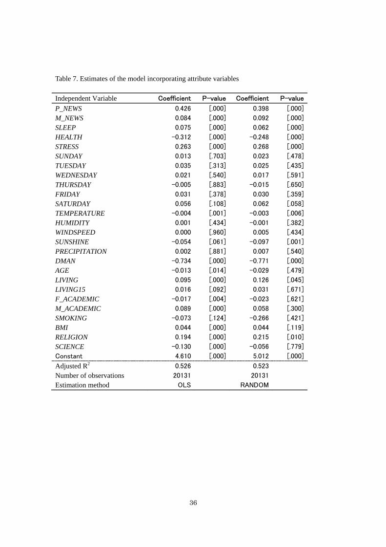
Estimation results for the model when these attributes are included are presented in Table
7. The number of observations decreases to 20,131. The left-hand columns show the results of
OLS estimation.15 The coefficients on all the variables of the basic equation are qualitatively
the same as those in Table 2, except that the coefficient on HUMIDITY becomes insignificant
15 Since the attributive variables have only one observation per subject, fixed effects models that include these variables cannot be estimated.
- 22 -
and that no coefficients on day-of-the-week dummies are significant.
Most of the attributes are significant, and the signs of their coefficients are consistent with
intuition and with previous studies (e.g. Frey and Stutzer 2002). Females are happier than males,
and younger students are happier than older students. Higher current and past standards of living
are positively correlated with happiness. Those whose mothers have more education are happier,
while for fathers the result is the opposite.16 The coefficient on SMOKING is negative but
insignificant (possibly due to the fact that there were no heavy smokers). Higher BMI is
correlated with higher happiness. Religious people are happier. Those who belong to science
departments are unhappier than those affiliated with humanities and social science departments.
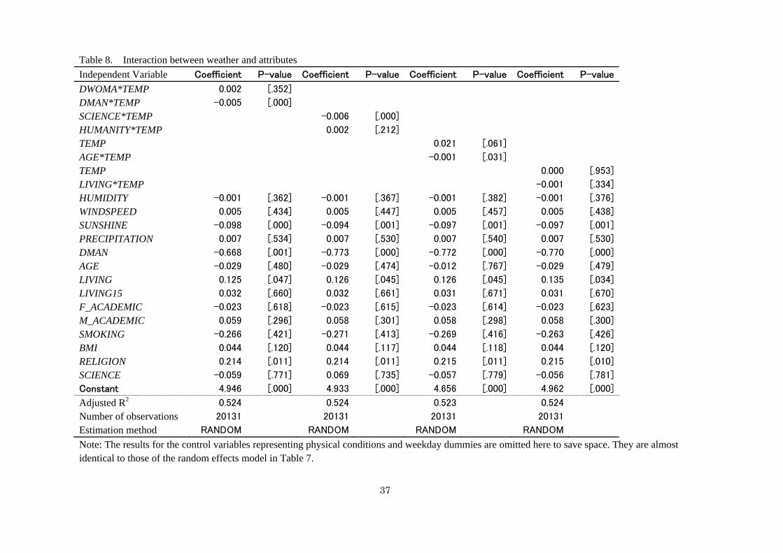
It is interesting to ask whether the sensitivity of happiness to weather conditions differs
depending on a respondent’s attributes. To check this, I constructed cross terms between the
attributes and TEMPERATURE and added these to the extended equation shown in Table 7. The
estimation results are presented in Table 8. Estimates for variables of physical condition and
day-of-the-week dummies are omitted to save space, since they are almost the same as those in
Table 7. In the first column, cross terms between female and male dummies and
TEMPERATURE (DWOMAN*TEMP and DMAN*TEMP) are added. Interestingly, only males
prefer low temperatures, while females are not affected by temperature, which is consistent with
16 This result is not easy to interpret.
- 23 -
the result of Barston (1988).
In the second column, cross terms between TEMPERATRE and academic department
dummies (SCIENCE*TEMP and HUMANITY*TEMP) are added. Science majors are negatively
affected by higher temperatures, while humanities majors show insignificant sensitivity. This
may simply be due to the fact that science majors contain a much higher percentage of males
than humanities departments.
In the third column, a cross term between AGE and TEMPERATURE is added. The cross
term is significantly negative at the 5% level, indicating that older students dislike high
temperatures more. In the fourth column, a cross term between living standard and
TEMPERATURE is added; however, living standard does not affect sensitivity to temperature.
In sum, the sensitivity of happiness to temperature does depend on certain individual
attributes.
4.5 Hourly weather data vs. daily average weather data
Various specifications, including the basic equation, have so far been estimated with hourly
weather data on the right-hand side. However, it might be the case that happiness is influenced
more by overall weather over the course of a day than by weather at the exact time of the survey.
To investigate this possibility, I re-estimated the basic equation with daily weather data.
- 24 -
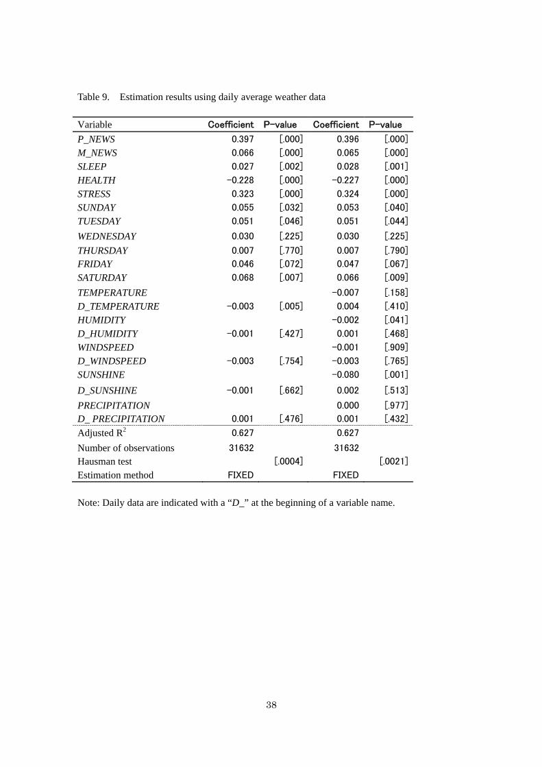
Estimation results using daily data for Osaka city are presented in the left-hand columns of
Table 9. In the table, a daily average weather variable is identified with a “D_” at the beginning
of the variable name. D_TEMPERATURE, D_HUMIDITY, and D_WINDSPEED are daily
averages, while D_SUNSHINE and D_PRECIPITATION are total daily amounts.
The estimates for the control variables, including day-of-the-week dummies, are almost
identical to the estimates in the specifications using hourly weather data. However, the estimates
for meteorological variables are somewhat different. Among them, D_TEMPERATURE is only
noteworthy at the 1% significance level (Table 9); the other four variables are not significant at
all. Comparing these results with those obtained with hourly data suggests that hourly data have
a stronger effect on HAPPINESS than do daily average data, and that the effect of temperature is
the most robust.
To further examine the former suggestion, I estimated a regression incorporating both
hourly and daily meteorological variables, shown in the right-hand columns of Table 9. Hourly
data are significant for humidity and sunshine, while daily data are not, suggesting that the
former has more explanatory power. For temperature, both hourly and daily data are
insignificant; however, the hourly data have a negative coefficient (p-value of 15%), while the
daily data take a positive sign. These results support the notion that hourly data have more
explanatory power, suggesting that happiness depends on current weather rather than on average
- 25 -
weather over a day.
4.6 Impact of weather on other affect variables
In the questionnaire, I solicited additional measures of positive and negative affect. The first of
these is “(Q2) Are you sad now?” Possible responses to this question are 1 (sad), 2 (somewhat
sad), 3 (somewhat not sad), and 4 (not sad). I define the variable SADNESS as the answer to this
question. The second is “(Q3) Are you enjoying life now?” Possible responses are 1 (enjoying
life), 2 (somewhat enjoying life), 3 (somewhat not enjoying life), and 4 (not enjoying life). I
define the variable ENJOYMENT as 5 minus the answer to this question. Finally, respondents
were asked “(Q4) Are you depressed now?” They had four possible responses: 1 (very
depressed), 2 (somewhat depressed), 3 (somewhat not depressed), and 4 (not depressed). I
define the variable DEPRESSION as the answer to this question. Note that all of these variables
are defined so that a higher value indicates a more positive affect. It is interesting to ask how
these variables are affected by the weather.
In Table 1, descriptive statistics for SADNESS, PLEASURE, and DEPRESSION are
shown. The correlation coefficients between HAPPINESS and these three variables range from
0.4 to 0.6. The correlations between these affect variables and the various conditions of the
subjects are quite similar to those of HAPPINESS. However, the correlations of these affect
- 26 -
measures with the meteorological variables are slightly different from those of HAPPINESS.
For example, the correlation with humidity is positive for ENJOYMENT and DEPRESSION,
while it is negative for other measures of affect.
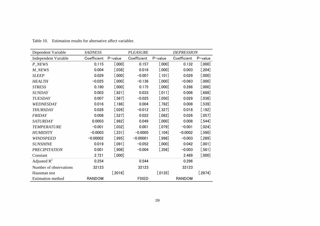
In Table 10, I present regression results for the basic model using these three measures as
the dependent variable. Results for negative affect variables, SADNESS and DEPRESSION, are
consistent with the results for HAPPINESS, in that temperature has a negative effect on
happiness. However, SUNSHINE has positive effects on SADNESS and DEPRESSION. On the
other hand, positive affect, PLEASURE, behaves somewhat differently. Higher temperature
correlates with higher PLEASURE, which is the opposite of the outcome for HAPPINESS. Thus,
the effects of meteorological variables on well-being depend on how well-being is measured.
5. Conclusions
This paper investigates the time-series dependence of happiness on weather for individuals
living in a single location, while most earlier studies examine the effects of differing climates on
geographically dispersed populations. Although there are some studies that focus on how daily
weather affects mood, the present study is unique in that the data covers 17 months, which is
much longer than the six weeks or less covered in previous studies. Additionally, this study
includes detailed data on the individual attributes, physical conditions, and daily experiences of
- 27 -
the respondents, which allow more robust controls than in past studies.
Empirical analysis reveals that happiness is negatively related to temperature in a linear
model, and is maximized at 13.9 degrees Celsius in a quadratic model. Humidity and sunshine
also have a negative effect on happiness; however, the result for sunshine is found to be
spurious: the effect is entirely due to the fact that sunshine is zero at night and people are
happier at night. The other meteorological variables, wind speed, and precipitation, do not
significantly affect happiness.
I check the robustness of my results in various ways. The survey I use does not identify
the exact locations of respondents; however, all of the respondents were students of Osaka
University, so that they stayed near campus for most of the sample period. Using subjects’
reports on travel and class attendance, I showed that the use of Osaka city weather data does not
produce large biases. In addition, using detailed data on subjects’ attributes, I found that the
sensitivity of happiness to temperature depends on attributes such as sex, age and academic
major. It is also the case that happiness is more strongly affected by current hourly weather than
by averaged weather over the entire day. Finally, while negative affect is affected by weather in
a similar way to happiness, positive affect behaves in a somewhat different manner.
- 28 -
References
Barnston, A. G. (1988). The effect of weather on mood, productivity, and frequency of
emotional crisis in a temperate continental climate. International Journal of Biometeorology, 32,
134-143.
Bigano, A., Bosello, F., Roon, R., & Tol, R. S. J. (2008). Economy-wide impacts of climate
change: A joint analysis for sea level rise and tourism. Mitigation and Adaptation Strategies for
Global Change, 13, 765–791.
Brereton, F., Clinch, J.P., & Ferreira, S., (2008). Happiness, geography and the environment.
Ecological Economics, 65 (2), 386-396.
Denissen, J. J. A., Butalid, L., Penke, L., & van Aken, M. A. G. (2008). The effects of weather
on daily mood: A multilevel approach. Emotion, 8, 662–667.
Dolan, P., Peasgood, T., & White, M. (2008). Do we really know what makes us happy? A
review of the economic literature on the factors associated with subjective well-being. Journal
of Economic Psychology, 29, 94–122.
Eisinga, R., Franses, P. H. & Vergeer, M. (2011). Weather conditions and daily television use in
the Netherlands, 1996–2005, International Journal of Biometeorology, 55, 555–564.
Frey, B. S., & Stutzer, A. (2002). What can economists learn from happiness research? Journal
of Economic Literature, 40(2), 402–435.
Frijters, P., & Van Praag, B. M. S. (1998). The effects of climate on welfare and well-being in
Russia. Climatic Change, 39, 61–81.
Hoch, I., & Drake, J. (1974). Wages, climate, and the quality of life. Journal of Environmental
Economics and Management, l, 268–295.
Huibers, M.J.H., Esther de Graaf, L., Peeters, F. P. M. L., & Arntz, A. (2010). Does the weather
make us sad? Meteorological determinants of mood and depression in the general population.
Psychiatry Research, 180, 143–146.
Kahneman, D., Kruger, A. B., Schkade, D. A., Schwartz, N., & Stone, A.A. (2004). A survey
method for characterizing daily life experience: The day reconstruction method. Science, 306,
- 29 -
1776-1780.
Kämpfer, S. & Mutz, M. (2011). On the sunny side of life: Sunshine effects on life satisfaction.
Social Indicators Research, available online.
Klimstra, T. A., Frijns, T., Keijsers, L., Denissen, J. J. A., Raaijmakers, Q. A. W., van Aken, M.
A. G., Koot, H. M., van Lier, P. A. C. & Meeus, W. H. J. (2011). Come rain or come shine:
Individual differences in how weather affects mood. Emotion, 11 (6), 1495–1499.
Kööt, L., Realo, A., & Allik, J. (2011). The influence of the weather on affective experience: An
experience sampling study. Journal of Individual Differences, 32 (2), 74-84.
Maddison, D. J. (2003). The amenity value of climate: The household production function
approach. Resource and Energy Economics, 25, 155–175.
Maddison, D. J., & Bigano, A. (2003). The amenity value of the Italian climate. Journal of
Environmental Economics and Management, 45, 319–332.
Moro, M., Brereton, F., Ferreira, S., Clinch, J. P. (2008). Ranking quality of life using
subjective well-being data. Ecological Economics, 65(3): 448-460.
Oswald, A. J. and Wu, S. (2010). Objective confirmation of subjective measures of human
well-being: Evidence from the U.S.A. Science, 327 (5965), 576-579.
Rehdanz, K., & Maddison, D. (2005). Climate and happiness. Ecological Economics, 52, 11–
125.
Schwarz, N. and Clore, G. L. (1983). Mood, misattribution and judgments of well-being:
information and directive functions of affective states. Journal of Personality and Social
Psychology, 45, 513-23.
Tselepidaki, I. M., Santamouris, C. M., & Poulopoulou, G. (1992). Analysis of the summer
discomfort index in Athens, Greece, for cooling purposes. Energy and Buildings, 18, 51–56.
Van Praag, B. M. S. (1988). Climate equivalence scales. European Economic Review, 32, 1019–
1024.
30
Table 1. Descriptive statistics
CORRELATION with
Mean Std Dev Minimum Maximum HAPPINESS SADNESS ENJOYMENT DEPRESSION
HAPPINESS 5.867 1.972 0 10 1
SADNESS 3.172 0.853 1 4 0.501 1
ENJOYMENT 2.450 0.907 1 4 0.597 0.357 1
DEPRESSION 3.075 0.949 1 4 0.448 0.728 0.362 1
P_NEWS 0.522 2.355 -5 5 0.644 0.415 0.542 0.439
M_NEWS -0.415 2.043 -5 5 0.183 0.112 0.117 0.137
SLEEP 2.616 0.976 1 4 0.172 0.190 0.080 0.161
HEALTH 2.270 0.787 1 4 -0.308 -0.289 -0.233 -0.307
STRESS 2.005 0.911 1 4 0.403 0.392 0.298 0.427
TEMPERATURE 15.103 8.126 -0.1 36.9 -0.044 -0.030 -0.021 -0.038
HUMIDITY 61.245 14.344 15 94 -0.001 -0.006 0.009 0.001
WINDSPEED 2.385 1.306 0 9.9 -0.008 -0.0001 -0.007 -0.009
SUNSHINE 0.201 0.366 0 1 -0.031 -0.004 -0.053 -0.015
PRECIPITATION 0.117 0.807 0 26 0.0002 -0.003 -0.0002 -0.004
Note: The number of observations is 32125.
31
Table 2. Estimation results for the basic equation
Variable Coefficient P-value Coefficient P-value Coefficient P-value Coefficient P-value
P_NEWS 0.397 [.000] 0.397 [.000] 0.374 [.000]
M_NEWS 0.065 [.000] 0.065 [.000] 0.063 [.000]
SLEEP 0.029 [.001] 0.028 [.001] 0.038 [.007]
HEALTH -0.227 [.000] -0.227 [.000] -0.302 [.000]
STRESS 0.322 [.000] 0.322 [.000] 0.406 [.000]
SUNDAY 0.051 [.044] 0.053 [.036] 0.066 [.130]
TUESDAY 0.046 [.066] 0.046 [.066] -0.010 [.811]
WEDNESDAY 0.030 [.228] 0.029 [.245] 0.037 [.363]
THURSDAY 0.005 [.833] 0.006 [.818] -0.009 [.831]
FRIDAY 0.048 [.056] 0.048 [.056] 0.016 [.702]
SATURDAY 0.064 [.010] 0.065 [.010] 0.066 [.120]
TEMPERATURE -0.003 [.003] -0.009 [.000] 0.012 [.002] -0.003 [.035]
TEMP_SQ -0.00042 [.000]
HUMIDITY -0.001 [.039] -0.002 [.004] -0.001 [.058] -0.002 [.100]
WINDSPEED -0.003 [.620] 0.007 [.331] -0.001 [.837] 0.003 [.701]
SUNSHINE -0.080 [.000] -0.144 [.000] -0.076 [.001] 0.002 [.951]
PRECIPITATION 0.001 [.929] 0.000 [.969] -0.002 [.831] -0.014 [.466]
Constant 6.158 [.000]
Adjusted R2 0.628 0.002 0.628 0.651
Number of observations 32123 32123 32123 12187
Hausman test [.0006] [.2046] [.0011] [.0044]
Estimation method FIXED RANDOM FIXED FIXED
Note: On the basis of the results of the Hausman test and the F-test of the same constant, estimates of the random effects models are presented
in the second columns and estimates of the fixed effects model in the other columns.
32
Table 3. Estimation results using Toyonaka city data for temperature, wind speed, and precipitation
Independent Variable Coefficient P-value Coefficient P-value
P_NEWS 0.397 [.000] 0.397 [.000]
M_NEWS 0.065 [.000] 0.065 [.000]
SLEEP 0.029 [.001] 0.028 [.001]
HEALTH -0.227 [.000] -0.227 [.000]
STRESS 0.322 [.000] 0.321 [.000]
SUNDAY 0.052 [.040] 0.056 [.027]
TUESDAY 0.047 [.062] 0.047 [.059]
WEDNESDAY 0.030 [.223] 0.030 [.228]
THURSDAY 0.006 [.799] 0.009 [.726]
FRIDAY 0.049 [.051] 0.050 [.045]
SATURDAY 0.065 [.009] 0.067 [.007]
T_TEMPERATURE -0.002 [.006] -0.003 [.000]
HUMIDITY -0.001 [.048]
T_WINDSPEED -0.004 [.368] -0.003 [.413]
SUNSHINE -0.079 [.000]
T_ PRECIPITATION -0.003 [.653] -0.004 [.536]
Adjusted R2 0.628 0.628
Number of observations 32111 32111
Hausman test [.0015] [.0008]
Estimation method FIXED FIXED
Note: T_TEMPERATURE, T_WINDSPEED, and T_PRECIPITATION indicate that the data are those of Toyonaka city. On the basis of the results of the Hausman test and the F-test of the same constant, estimates of the fixed effects model are presented.
33
Table 4. Estimates for summer and winter samples
Summer Winter
Independent Variable Coefficient P-value Coefficient P-value Coefficient P-value Coefficient P-value
P_NEWS 0.383 [.000] 0.383 [.000] 0.416 [.000] 0.417 [.000]
M_NEWS 0.076 [.000] 0.077 [.000] 0.059 [.000] 0.059 [.000]
SLEEP 0.016 [.234] 0.016 [.256] 0.026 [.020] 0.025 [.024]
HEALTH -0.168 [.000] -0.167 [.000] -0.222 [.000] -0.222 [.000]
STRESS 0.261 [.000] 0.260 [.000] 0.330 [.000] 0.330 [.000]
SUNDAY 0.046 [.256] 0.052 [.203] 0.051 [.125] 0.052 [.115]
TUESDAY 0.046 [.256] 0.045 [.262] 0.054 [.103] 0.054 [.097]
WEDNESDAY 0.040 [.321] 0.038 [.335] 0.037 [.261] 0.035 [.291]
THURSDAY 0.010 [.803] 0.011 [.784] 0.006 [.857] 0.010 [.772]
FRIDAY 0.045 [.271] 0.049 [.222] 0.045 [.170] 0.046 [.163]
SATURDAY 0.093 [.022] 0.096 [.017] 0.049 [.131] 0.049 [.133]
TEMPERATURE -0.003 [.153] -0.005 [.031] 0.005 [.024] 0.004 [.036]
HUMIDITY -0.0004 [.685] -0.001 [.069]
WINDSPEED -0.0003 [.977] -0.004 [.537]
SUNSHINE -0.074 [.053] -0.074 [.010]
PRECIPITATION 0.001 [.938] 0.008 [.727]
Adjusted R2 0.647 0.672 0.647 0.647
Number of observations 11187 11187 17745 17745
Hausman test [.0012] [.0006] [.0024] [.0012]
Estimation method FIXED FIXED FIXED FIXED

34
Table 5. Effect of class attendance and weekend on the sensitivity to temperature
Independent Variable Coefficient P-value Coefficient P-value Coefficient P-value
P_NEWS 0.521 [.000] 0.431 [.000] 0.397 [.000]
M_NEWS -0.010 [.872] 0.060 [.000] 0.065 [.000]
SLEEP -0.099 [.451] 0.014 [.362] 0.029 [.001]
HEALTH -0.198 [.217] -0.158 [.000] -0.227 [.000]
STRESS 0.505 [.000] 0.187 [.000] 0.322 [.000]
CLASS -0.101 [.123]
SUNDAY 0.520 [.191] 0.017 [.702] 0.053 [.157]
TUESDAY 0.560 [.187] -0.035 [.423] 0.046 [.066]
WEDNESDAY 0.077 [.871] 0.031 [.474] 0.030 [.228]
THURSDAY 0.095 [.812] -0.006 [.897] 0.005 [.833]
FRIDAY 0.581 [.127] 0.025 [.558] 0.048 [.056]
SATURDAY 0.452 [.231] 0.046 [.284] 0.066 [.076]
TEMPERATURE 0.004 [.771] 0.007 [.072] -0.002 [.014]
CLASS*TEMP 0.003 [.670]
WEEKEND*TEMP -0.0001 [.950]
HUMIDITY -0.006 [.512] -0.001 [.244] -0.001 [.039]
WINDSPEED 0.099 [.260] 0.006 [.487] -0.003 [.618]
SUNSHINE 0.247 [.634] -0.159 [.000] -0.080 [.000]
PRECIPITATION -0.154 [.592] -0.030 [.282] 0.001 [.929]
Constant 4.969 [.000]
Adjusted R2 0.398 0.761 0.628
Number of observations
147 7459 32123
Hausman test [.3275] [.0003] [.0010]
Estimation method RANDOM FIXED FIXED
Note: In the left-hand columns, estimation results are presented where only traveling days are used. The observation period for the results shown in the middle columns is from December 1, 2007 to March 31, 2008. The coefficient on TEMPERATURE is positive, since the estimation period is “winter”.
35
Table 6. Descriptive statistics of attribute variables
Mean Std Dev Minimum Maximum
DMAN 0.691 0.466 0 1
AGE 21.545 2.026 18 28
LIVING 5.236 1.563 1 8
LIVING15 5.400 1.461 2 8
F_ACADEMIC 5.745 2.382 2 11
M_ACADEMIC 4.618 1.769 1 9
SMOKING 1.055 0.229 1 2
BMI 20.841 2.883 15.397 33.412
RELIGION 1.473 1.052 1 5
SCIENCE 0.600 0.494 0 1
Note: The number of observations is 55.
36
Table 7. Estimates of the model incorporating attribute variables
Independent Variable Coefficient P-value Coefficient P-value
P_NEWS 0.426 [.000] 0.398 [.000]
M_NEWS 0.084 [.000] 0.092 [.000]
SLEEP 0.075 [.000] 0.062 [.000]
HEALTH -0.312 [.000] -0.248 [.000]
STRESS 0.263 [.000] 0.268 [.000]
SUNDAY 0.013 [.703] 0.023 [.478]
TUESDAY 0.035 [.313] 0.025 [.435]
WEDNESDAY 0.021 [.540] 0.017 [.591]
THURSDAY -0.005 [.883] -0.015 [.650]
FRIDAY 0.031 [.378] 0.030 [.359]
SATURDAY 0.056 [.108] 0.062 [.058]
TEMPERATURE -0.004 [.001] -0.003 [.006]
HUMIDITY 0.001 [.434] -0.001 [.382]
WINDSPEED 0.000 [.960] 0.005 [.434]
SUNSHINE -0.054 [.061] -0.097 [.001]
PRECIPITATION 0.002 [.881] 0.007 [.540]
DMAN -0.734 [.000] -0.771 [.000]
AGE -0.013 [.014] -0.029 [.479]
LIVING 0.095 [.000] 0.126 [.045]
LIVING15 0.016 [.092] 0.031 [.671]
F_ACADEMIC -0.017 [.004] -0.023 [.621]
M_ACADEMIC 0.089 [.000] 0.058 [.300]
SMOKING -0.073 [.124] -0.266 [.421]
BMI 0.044 [.000] 0.044 [.119]
RELIGION 0.194 [.000] 0.215 [.010]
SCIENCE -0.130 [.000] -0.056 [.779]
Constant 4.610 [.000] 5.012 [.000]
Adjusted R2 0.526 0.523
Number of observations 20131 20131
Estimation method OLS RANDOM
37
Table 8. Interaction between weather and attributes
Independent Variable Coefficient P-value Coefficient P-value Coefficient P-value Coefficient P-value
DWOMA*TEMP 0.002 [.352]
DMAN*TEMP -0.005 [.000]
SCIENCE*TEMP -0.006 [.000]
HUMANITY*TEMP 0.002 [.212]
TEMP 0.021 [.061]
AGE*TEMP -0.001 [.031]
TEMP 0.000 [.953]
LIVING*TEMP -0.001 [.334]
HUMIDITY -0.001 [.362] -0.001 [.367] -0.001 [.382] -0.001 [.376]
WINDSPEED 0.005 [.434] 0.005 [.447] 0.005 [.457] 0.005 [.438]
SUNSHINE -0.098 [.000] -0.094 [.001] -0.097 [.001] -0.097 [.001]
PRECIPITATION 0.007 [.534] 0.007 [.530] 0.007 [.540] 0.007 [.530]
DMAN -0.668 [.001] -0.773 [.000] -0.772 [.000] -0.770 [.000]
AGE -0.029 [.480] -0.029 [.474] -0.012 [.767] -0.029 [.479]
LIVING 0.125 [.047] 0.126 [.045] 0.126 [.045] 0.135 [.034]
LIVING15 0.032 [.660] 0.032 [.661] 0.031 [.671] 0.031 [.670]
F_ACADEMIC -0.023 [.618] -0.023 [.615] -0.023 [.614] -0.023 [.623]
M_ACADEMIC 0.059 [.296] 0.058 [.301] 0.058 [.298] 0.058 [.300]
SMOKING -0.266 [.421] -0.271 [.413] -0.269 [.416] -0.263 [.426]
BMI 0.044 [.120] 0.044 [.117] 0.044 [.118] 0.044 [.120]
RELIGION 0.214 [.011] 0.214 [.011] 0.215 [.011] 0.215 [.010]
SCIENCE -0.059 [.771] 0.069 [.735] -0.057 [.779] -0.056 [.781]
Constant 4.946 [.000] 4.933 [.000] 4.656 [.000] 4.962 [.000]
Adjusted R2 0.524 0.524 0.523 0.524
Number of observations 20131 20131 20131 20131
Estimation method RANDOM RANDOM RANDOM RANDOM
Note: The results for the control variables representing physical conditions and weekday dummies are omitted here to save space. They are almost identical to those of the random effects model in Table 7.
38
Table 9. Estimation results using daily average weather data
Variable Coefficient P-value Coefficient P-value
P_NEWS 0.397 [.000] 0.396 [.000]
M_NEWS 0.066 [.000] 0.065 [.000]
SLEEP 0.027 [.002] 0.028 [.001]
HEALTH -0.228 [.000] -0.227 [.000]
STRESS 0.323 [.000] 0.324 [.000]
SUNDAY 0.055 [.032] 0.053 [.040]
TUESDAY 0.051 [.046] 0.051 [.044]
WEDNESDAY 0.030 [.225] 0.030 [.225]
THURSDAY 0.007 [.770] 0.007 [.790]
FRIDAY 0.046 [.072] 0.047 [.067]
SATURDAY 0.068 [.007] 0.066 [.009]
TEMPERATURE -0.007 [.158]
D_TEMPERATURE -0.003 [.005] 0.004 [.410]
HUMIDITY -0.002 [.041]
D_HUMIDITY -0.001 [.427] 0.001 [.468]
WINDSPEED -0.001 [.909]
D_WINDSPEED -0.003 [.754] -0.003 [.765]
SUNSHINE -0.080 [.001]
D_SUNSHINE -0.001 [.662] 0.002 [.513]
PRECIPITATION 0.000 [.977]
D_ PRECIPITATION 0.001 [.476] 0.001 [.432]
Adjusted R2 0.627 0.627
Number of observations 31632 31632
Hausman test [.0004] [.0021]
Estimation method FIXED FIXED
Note: Daily data are indicated with a “D_” at the beginning of a variable name.
39
Table 10. Estimation results for alternative affect variables
Dependent Variable SADNESS PLEASURE DEPRESSION
Independent Variable Coefficient P-value Coefficient P-value Coefficient P-value
P_NEWS 0.115 [.000] 0.157 [.000] 0.132 [.000]
M_NEWS 0.004 [.038] 0.016 [.000] 0.003 [.204]
SLEEP 0.029 [.000] -0.007 [.101] 0.029 [.000]
HEALTH -0.025 [.000] -0.136 [.000] -0.063 [.000]
STRESS 0.190 [.000] 0.175 [.000] 0.286 [.000]
SUNDAY 0.003 [.821] 0.033 [.011] 0.006 [.688]
TUESDAY 0.007 [.567] -0.025 [.050] 0.029 [.036]
WEDNESDAY 0.016 [.186] 0.004 [.782] 0.008 [.539]
THURSDAY 0.028 [.026] -0.012 [.327] 0.018 [.192]
FRIDAY 0.008 [.527] 0.022 [.082] 0.026 [.057]
SATURDAY 0.0003 [.982] 0.049 [.000] 0.008 [.544]
TEMPERATURE -0.001 [.032] 0.001 [.079] -0.001 [.024]
HUMIDITY -0.0003 [.231] -0.0005 [.104] -0.0002 [.590]
WINDSPEED -0.00002 [.995] -0.00001 [.998] -0.003 [.289]
SUNSHINE 0.019 [.091] -0.052 [.000] 0.042 [.001]
PRECIPITATION 0.001 [.908] -0.004 [.356] -0.003 [.561]
Constant 2.721 [.000] 2.489 [.000]
Adjusted R2 0.254 0.544 0.296
Number of observations 32123 32123 32123
Hausman test [.2016] [.0135] [.2874]
Estimation method RANDOM FIXED RANDOM

40
Figure 1. Map of three locations: two campuses of Osaka University and Osaka city
Osaka University Toyonaka Campus
Osaka University Suita Campus
Osaka City
41
Figure 2. Average temperature of Osaka city
0
5
10
15
20
25
30
35


