Download - Gate Sizing by Lagrangian Relaxation Revisitedjwang/gs_iccad07_talk.pdf · Gate Sizing by Lagrangian Relaxation Revisited Jia Wang, Debasish Das, and Hai Zhou Electrical Engineering

Gate Sizing by Lagrangian Relaxation Revisited

Jia Wang, Debasish Das, and Hai ZhouElectrical Engineering and Computer Science

Northwestern UniversityEvanston, Illinois, United States

October 17, 2007

1 / 41

Outline

Introduction to Gate Sizing

Generalized Convex Sizing

The Dual Problems

The DualFD Algorithm

Experiments

Conclusions

2 / 41

Gate Sizing

I A mathematical programming formulation.I Timing constraints: delays, arrival times.I Objective function: clock period, total weighted area, etc.

I Trade off performance and cost.I Optimize performance.I Optimize cost under performance constraint.

3 / 41

Previous Works – General Convex Optimization

TILOS [Fishburn & Dunlop, ’85], [Sapatnekar et al., ’93], etc.

I Transform sizing into a convex programming problem.I Assume convex delays (after variable transformation).I Convexity through geometric programming commonly.

I Apply general convex optimization techniques.I Studied for decades.I High running time.

4 / 41

Previous Works – Lagrangian Relaxation

[Chen, Chu, & Wong, ’99], [Tennakoon & Sechen, ’02, ’05]

I Special structure:timing constraints are system of difference inequalities.

I The Lagrangian dual problem is simplified.I Objective function (Lagrangian dual function):

available through Lagrangian subproblems.I Constraints: flow conservation on Lagrangian multipliers.

I Lagrangian dual function is not differentiable in general.Apply subgradient optimizations.

I Difficult to choose good initial solution and step sizes.I Pre-processing can help choosing initial solutions for some

delay models.I No universal pre-processing method for all convex delays.

5 / 41

Contribution

I Combine gate sizing with sequential optimization.I Revisit Lagrangian relaxation.

I Correct misunderstandings.I Check primal feasibility in dual problems.

I Identify a class of problems with differentiable dual functions.I The DualFD algorithm: use gradient and network flow.

6 / 41

Outline



The Dual Problems


Experiments

Conclusions

7 / 41

Generalized Convex Sizing (GCS)

Minimize C (x)

s.t. ti + di ,j(x)− tj ≤ 0,∀(i , j) ∈ E ,

x ∈ Ω.

I G = (V ,E ): a directed graph, the system structure.

I x: the system parameters belonging to

Ω∆= x : lk ≤ xk ≤ uk ,∀1 ≤ k ≤ n.

I t: (relative) arrival times.

I C (x), di ,j(x): objective function and delays, twicedifferentiable and convex.

8 / 41

The GCS Formulation

I Timing specification in sequential circuits.

Feasible timing ⇔ No positive cycle

I Prefer edge delays to vertex delays for accuracy.I Timing arcs in one gate/cell.I Rise/fall delay and slew.

I Flexibility in choosing x.I Logarithms of sizes (gate, wire, transistor, etc. )for Elmore and

posynomial delays.I Clock skews and clock period.

9 / 41

GCS is Convex

I GCS formulation is convex.I Objective function and feasible set are convex.I Not necessary to establish convexity through geometric

programming.

I Non-convex formulations can be transformed into convexones.

I Properties of convex formulations are not necessarily hold forequivalent non-convex ones.

10 / 41

Proper GCS Problems

DefinitionA GCS is proper iff:

∀x ∈ Ω,∀z 6= 0, z>HC (x)z 6= 0.

I With differentiable dual functions (shown later).I di,j(x) are irrelevant.

I Optimizing total positive weighted area is proper.

11 / 41

Simultaneous Sizing and Clock Skew Optimization

I Minimize total area under performance bound while allowingclock skew optimization.

I Handle long path conditions (setup condition).

I Assume post-processing for repairing of violated short pathconditions (hold condition).

I Not proper: ∂C∂s = 0,∀clock skew variable s.

I Cancel s. Transform to a proper one.

12 / 41

Simultaneous Sizing and Clock Skew OptimizationMake a Non-Proper Problem Proper

I Constraints concerning clock skew sk :

(tI + sk ≤ tQk) ∧ (tDk

− sk ≤ tO) ∧ (s−k ≤ sk ≤ s+k )

I Cancel sk : [tDk− tO, tQk

− tI]∩[s−k , s+k ] 6= ∅. Equivalently:

(tDk− s+

k ≤ tO) ∧ (tI + s−k ≤ tQk) ∧ (tDk

− tQk≤ T )

13 / 41

Outline



The Dual Problems


Experiments

Conclusions

14 / 41

Lagrangian Relaxation Overview

I Lagrangian function:

L∗(x, t, f) = C (x) +∑

(i ,j)∈E

fi ,j(ti + di ,j(x)− tj)

I Lagrangian subproblem:

L(f) = infL∗(x, t, f) : x ∈ Ω, t ∈ R |V |

I Lagrangian dual problem (D-GCS):

Maximize L(f)

s.t. f ∈ N .

N : non-negative f.

15 / 41

Duality Gap

P∆= infC (x) : x ∈ X,D ∆

= supL(f) : f ∈ N.

X : feasible x.

I Zero duality gap is necessary: P = D.

I Establish P = D through Strong Duality Theorem.I Strictly feasible solution ⇒ exists saddle point (x, t, f):

D = L(f) = L∗(x, t, f) = C (x) = P.

I Misunderstanding: previous work applied Strong DualityTheorem to original non-convex formulation (transformationwas necessary for convexity).

I GCS is convex without transformation.

16 / 41

Duality Gap

P∆= infC (x) : x ∈ X,D ∆

= supL(f) : f ∈ N.

X : feasible x.

I Zero duality gap is necessary: P = D.I Establish P = D through Strong Duality Theorem.

I Strictly feasible solution ⇒ exists saddle point (x, t, f):

D = L(f) = L∗(x, t, f) = C (x) = P.

I Misunderstanding: previous work applied Strong DualityTheorem to original non-convex formulation (transformationwas necessary for convexity).

I GCS is convex without transformation.

16 / 41

Duality Gap

I What if there is no strictly feasible solution?

I Regularity condition ⇒ zero duality gap. [Rockafellear 1971]

I More general than Strong Duality Theorem for zero dualitygap.

I No guarantee for saddle points as Strong Duality Theorem.

∀f ∈ N , L(f) < D.

17 / 41

Simplify the Dual Problem

I Flow conservation on G :

F ∆= f :

∑(i ,k)∈E

fi ,k =∑

(k,j)∈E

fk,j ,∀k ∈ V .

I L(f) = −∞ for f /∈ F , since

∀f /∈ F ,M ∈ R, x ∈ Ω,∃t ∈ R |V |, L∗(x, t, f) < M.

I Simplify D-GCS into FD-GCS:

Maximize L(f)

s.t. f ∈ F ∩N .

I Misunderstanding: previous works obtained FD-GCS by theKarush-Kuhn-Tucker (KKT) conditions ∂L∗

∂tk= 0. However,

KKT conditions are not necessary conditions.

18 / 41

A trivial example that is not trivial.

Will the extreme cases happen for sizing?

I Optimal solutions do NOT satisfy KKT conditions.

I No saddle point.

∀f ∈ F ∩N , L(f) < D.

.

19 / 41


Optimize a single inverter with size ex and fixed driver/load:

Minimize ex

s.t. t1 + ex ≤ t2, t2 + e−x ≤ t3, t3 ≤ t1 + 2,

− ln 2 ≤ x ≤ ln 2.

I Single feasible solution x = 0.Optimal but not strictly feasible.

I KKT conditions cannot be satisfied by x = 0:

0 =∂L∗

∂x= ex + f1,2e

x − f2,3e−x = 1 + f1,2 − f2,3,

0 =∂L∗

∂t2= f2,3 − f1,2.

20 / 41


I Since f ∈ F ∩N , assume β = f1,2 = f2,3 = f3,1 ≥ 0.

I Compute L(f):

L(f) = q(β) =

1+β

2 , if 0 ≤ β < 13

2√1+1/β+1

, if β ≥ 13

I q(β) increases from 12 to 1 when β increases from 0 to +∞.

I Therefore,∀f ∈ F ∩N , L(f) < 1 = D.

21 / 41

Further Simplification of the Dual Problem

I Simplify L(f) given f ∈ F :

Pf(x)∆= C (x) +

∑(i ,j)∈E

fi ,jdi ,j(x),

Q(f)∆= infPf(x) : x ∈ Ω.

⇒ L(f) = Q(f),∀f ∈ F .

I SD-GCS:

Maximize Q(f)

s.t. f ∈ F ∩N .

I SD-GCS is different from FD-GCS.

I D-GCS, FD-GCS, SD-GCS are equivalent.

22 / 41

Infeasibility for GCS

I GCS can be infeasible: clock period is too small.

I C (x) is continuous and Ω is compact:

∃U,∀x ∈ Ω,C (x) ≤ U.

I Assume zero duality gap, GCS is feasible iff

∀f ∈ F ∩N ,Q(f) ≤ U.

23 / 41

Outline



The Dual Problems


Experiments

Conclusions

24 / 41

Differentiable Dual Objective Q(f)

I Sufficient condition (from textbook):

∃xf ∈ Ω,∀x ∈ Ω,Q(f) = Pf(xf) < Pf(x).

I Assume the condition is NOT satisfied.

∃x′ 6= x′′ ∈ Ω,Q(f) = Pf(x′) = Pf(x

′′)

⇒ ∀0 ≤ γ ≤ 1,Q(f) = Pf((1− γ)x′ + γx′′)

⇒ (x′′ − x′)>HPf(x′′ + x′

2)(x′′ − x′) = 0

⇒ (x′′ − x′)>HC (x′′ + x′

2)(x′′ − x′) = 0

GCS is NOT proper!I For proper GCS problems, Q(f) is differentiable, and

∂Q(f)

∂fi ,j= di ,j(xf).

25 / 41

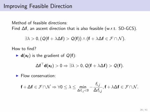
Improving Feasible Direction

Method of feasible directions:Find ∆f, an ascent direction that is also feasible (w.r.t. SD-GCS).

∃λ > 0, (Q(f + λ∆f) > Q(f)) ∧ (f + λ∆f ∈ F ∩N ).

How to find?

I d(xf) is the gradient of Q(f):

∆f>d(xf) > 0 ⇒ ∃λ > 0,Q(f + λ∆f) > Q(f).

I Flow conservation:

f +∆f ∈ F ∩N ⇒ ∀0 ≤ λ ≤ min∆fi,j<0

−fi ,j

∆fi ,j, f +λ∆f ∈ F ∩N .

26 / 41

Improving Feasible Direction

I The direction finding (DF) problem:

Maximize ∆f>d(xf)

s.t. f + ∆f ∈ F ∩N ,

−u ≤ ∆fi ,j ≤ u,∀(i , j) ∈ E .

∆f are decision variables, u is positive constant.

I ∆f>d(xf): first order approx. of Q(f + ∆f)− Q(f).

I DF is a min-cost network flow problem.

I For optimal ∆f, ∆f>d(xf) ≥ 0. And

∆f>d(xf) = 0 ⇒ xf is optimal for GCS.

27 / 41


I Iterative algorithm. Q(f) is increasing every iteration.I Q(f) is convex ⇒ local maximal is global maximum.I For subgradient optimizations, Q(f) may decrease.

I Each iteration,I Solve DF for ∆f.I Perform a line search to find Q(f + λ∆f) > Q(f)I Check GCS infeasibility when computing Q.I Claim optimality if the changes are marginal.

28 / 41

Outline



The Dual Problems


Experiments

Conclusions

29 / 41

Experimental Setup

I Minimize total area under performance bound with Elmoredelay model.

I ISCAS89 sequential circuits, 29 totally.Largest: ∼55000 vertices, ∼70000 edges, ∼21000 variables.

I Implement DualFD algorithm in C++.

I Use the CS2 min-cost network flow solver for DF. [Goldberg]

I Compare to subgradient optimizations: SubGrad.

30 / 41

Experimental Results

I 15 largest benchmarks.I Clock period achieved T vs. target clock period T0

I s838 is NOT feasible.

31 / 41

Experimental Results

I 15 largest benchmarks.

I Compare area, dual objective, and running time.

DualFD SubGradname area dual t(s) area dual t(s)s832 1060 1074 8.28 493 493 0.11s838 2916 80458 0.07 10189 -257K 51.51s953 776 775 5.92 3449 -80K 55.15s1196 1089 1088 10.90 1642 -14K 54.88s1238 1080 1080 7.80 974 -1823 27.19s1423 1668 1670 1.53 3346 -251K 120.76s1488 2055 2107 28.22 1150 557 31.28s1494 2161 2318 28.33 1140 529 32.02s5378 5856 6083 91.49 9396 -52K 308.39s9234 12935 15508 236.49 11517 -46K 384.86s13207 14608 14608 111.91 15642 -121K 432.81s15850 17766 17766 229.25 20628 -287K 600.10s35932 33522 44344 304.61 80650 -1M 600.34s38417 42176 44551 301.48 49126 -363K 600.35s38584 34973 34973 149.87 35016 -23K 600.19

32 / 41

DualFD vs. SubGrad

I 29 benchmarks totally.

I SubGrad never dominates DualFD.

33 / 41

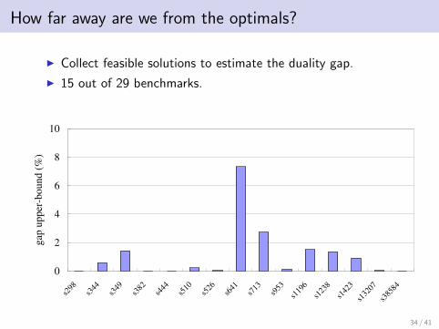
How far away are we from the optimals?

I Collect feasible solutions to estimate the duality gap.

I 15 out of 29 benchmarks.

34 / 41

Convergence of s38584

35 / 41

Outline



The Dual Problems


Experiments

Conclusions

36 / 41

Conclusions

I Formulate GCS problems to handle sequential optimization.

I Correct misunderstandings when applying Lagrangianrelaxation.

I Show how to detect infeasibility in GCS.

I Prove gradient exists for proposed proper GCS problems.

I Design the DualFD algorithm to solve proper GCS problems.

37 / 41

Q & A

38 / 41

Thank you!

39 / 41

L(f) vs. Q(f)

L(f) = Q(f), ∀f ∈ F ∩N ,

L(f) = −∞, ∀f ∈ N − F ,

Q(f) 6= −∞, ∀f ∈ N − F .

I L(f) is convex but not differentiable for f ∈ N .

I Q(f) is convex and differentiable for f ∈ N .

40 / 41

Proper GCS Problems

Posynomial objective functions of exk :

C (x) =l∑

i=1

ci eb>i x, ci > 0,∀1 ≤ i ≤ l

Let B = (b1,b2, . . . ,bl), rank(B) = n ⇔ proper.Full row rank.

41 / 41

Download - Gate Sizing by Lagrangian Relaxation Revisitedjwang/gs_iccad07_talk.pdf · Gate Sizing by Lagrangian Relaxation Revisited Jia Wang, Debasish Das, and Hai Zhou Electrical Engineering

Top Related