
1
FULBRIGHT VISITING REPORT RESEARCH ACTIVITIES
Analysis of Urban Structures Response to Ultra-High Frequency
Excitation from Close-in Blasting
DepartmentofCivilandEnvironmentalEngineeringNorthwesternUniversity–Evanston–Illinois(USA)
August 11, 2014 – February 10, 2015
Dr Essaieb Hamdi
Université de Tunis El Manar
Ecole Nationale d’Ingénieurs de Tunis
LR14ES03-Ingénierie Géotechnique
Civil Engineering Department
BP 37 Le Belvédère, 1002 Tunis. Tunisia
Phone: (216) 20 32 32 89
Email : [email protected]

ii
Acknowledgments
This report has been written during my Fulbright Visiting Research Stay at the Department of Civil and Envi-ronmental Engineering of Northwestern University (IL, USA). Special thanks go to the Fulbright Visiting Pro-gram selection committee at the US Embassy in Tunisia and in Washington DC and namely Mr. Sami Saaied from the US Embassy in Tunisia and Ms Ashley Gempp and Mr from the Council for International Exchange of Scholars (USA). I would like to thank Professor Charles H. Dowding for inviting me to this research stay at Northwestern Uni-versity, for his guidance, motivation, expertise, and foresight without which this work would certainly not have been possible. A lot of expertise has been acquired by me during this stay on construction and quarrying blast-ing operations and on how to measure and interpretate crack displacements and temperature measured by wire-less and wired systems. I am very grateful to Professor Catherine Aimone, Professor at New Mexico Institute of Mining and Technolo-gy and manager of Aimone-Martin Associates LLC. She gave me the opportunity to work on the New York City project which provided field experience for the analysis of blast induced vibrations from construction blasting. Pr Karen Chou is very thanked for her kindness towards me and for her very helpful assistance in the early steps of my stay. Special thanks go as well to Graig, Jennie, and George from the Infrastructure Technology Institute at North-western University for technical and administrative assistance provided during my stay. All colleagues that I met at the Nothwestern University, Yida, Montacer, Ferdinando, Constance, Ze Pei, Mehmet, Jo are very thanked for their friendship and the good atmosphere during my stay at Evanston. I cannot end without a thought to my wife Jihene, my children Mohamed Salah and Adem, my sisters Amira, Salma and Yosra and all my family and my wife’s family for the support and encouragement they have contin-ued to give me. I dedicate this report to the souls of my parents as a sign of reconnaissance of all education and principles they have given me.
Essaieb HAMDI

iii
Abstract
This report summarizes a case study that provides the multiple position, time correlated measurements
of structure response needed to advance the understanding of the response of larger urban structures to
ultra-high frequency blast induced excitation. While the first part of the report provides information to
determine the type of response, the second part provides the information concerning calculation of
strains and the distortion. The response is divided into three main chapters: Site & Instrumentation,
Time Histories, and Response. Site and Instrumentation is divided into three sections: site and geology,
transducers, and blasting practice. Time history is divided into three sections: attenuation, dominant fre-
quencies, and propagation. Structure Response is divided into two sections: amplification-
deamplification and response spectrum. The case study allowed the following conclusions: Urban struc-
tures respond predominantly in a wave transmission mode where there is noticeable difference in time,
frequency, phase, and amplitude of motions measured at the extreme top corners of the structure. Exci-
tation motions along the base are not the same; they differ significantly in time, frequency, and ampli-
tude. Excitation frequencies are so much larger than the natural frequencies of the structures and com-
ponents that the excitation motions were deamplified for all events.

iv
Content
Acknowledgments ......................................................................................................................................... iiAbstract ......................................................................................................................................................... iiiContent .......................................................................................................................................................... ivList of figures ................................................................................................................................................ viList of tables ................................................................................................................................................. viiIntroduction ................................................................................................................................................... 8
1Close-in blasting ...................................................................................................................................... 82Present study summary ............................................................................................................................ 9
Chapter 1. Site environment and building monitoring ............................................................................ 111Site and Geology .................................................................................................................................... 112Transducer description and installation ................................................................................................. 12
2.1 Building 1 transducers .................................................................................................................. 122.2 Building 2 transducers .................................................................................................................. 13
3Blasting practice ..................................................................................................................................... 14Chapter 2. Time histories analysis ............................................................................................................. 16
1Analysis methodology ............................................................................................................................ 162Blast-induced vibrations time histories .................................................................................................. 16
2.1 Attenuation of peak particle velocity ............................................................................................ 182.2 Ground vibration and frequency ................................................................................................... 19
3Propagation velocity in rock and structure ............................................................................................ 203.1 Rock wave velocity ...................................................................................................................... 203.2 Wave velocity within the structure ............................................................................................... 20
4Structure response to ultra high frequency excitation from close-in blasting ........................................ 214.1 Comparison of ground motion and structure response ................................................................. 214.2 Natural frequency and damping ratio ........................................................................................... 224.3 Amplification-deamplification ..................................................................................................... 234.1 Mid-wall versus upper structure amplification ............................................................................. 234.1 Comparison with wall and superstructure response measured by USBM .................................... 23
5Pseudo velocity response spectra demonstrate the expectaion of low distortion .................................. 255.1 Filtering and SDOF Calculation ................................................................................................... 25

v
5.2 Comparison with MS Excel 200-central moving average filtering .............................................. 275.3 Comparison with tunnel and quarrying blasts .............................................................................. 28
6Comparison of time correlated time histories illustrates wave transmission ......................................... 297Conclusion ............................................................................................................................................. 30
Chapter 3. Close-in blast induced strains ................................................................................................. 321Ground Motion Environment ................................................................................................................. 32
1.1 Integration of velocity time history .............................................................................................. 321.2 Differential displacement calculation ........................................................................................... 33
2Strain calculations .................................................................................................................................. 342.1 Procedure for calculating strains .................................................................................................. 342.3 Basement Wall response at building 2 ......................................................................................... 362.4 Comparison with ACM surveillance ............................................................................................ 372.5 Comparison with previous studies of tall structure response in urban close-in blasting .............. 38
3Strains versus Peak Particle Velocities .................................................................................................. 394Single-Degree-Of-Freedom response spectra ........................................................................................ 41
4.1 Displacement estimated from SDOF response spectrum ............................................................. 424.2 SDOF displacement versus PPV/freq and PPV ............................................................................ 464.1 Use of SDOF as Control Index ..................................................................................................... 484.2 Absolute displacement calculations .............................................................................................. 51
5Conclusions ............................................................................................................................................ 53References .................................................................................................................................................... 55Appendix A .................................................................................................................................................. 57Appendix B .................................................................................................................................................. 60

vi
List of figures
Figure 1. Blast locations with regards to the buildings. .................................................................................................................. 11Figure 2. Locations of the sensors at the upper and lower parts of the monitored walls at the two buildings. .............................. 13Figure 3. Simplified Sketch of the two buildings and a current blast ............................................................................................. 14Figure 4. Flowchart of the general methodology adopted for the buildings response analysis. ..................................................... 17Figure 5. Transmission of the ground motion to the lower transducer during blast 06/02. ............................................................ 17Figure 6. Transmission of the ground motion to the lower transducer during blast 06/02. ............................................................ 18Figure 7. Comparison of measured square root scaled distance attenuation and Oriard’s (1972) .................................................. 19Figure 8. Transit time estimation .................................................................................................................................................... 21Figure 9. Upper North transverse velocity time history recorded at Building 1 ............................................................................. 22Figure 10. Peak velocities for radial ground motion and north lower radial component ................................................................ 24Figure 11. Instrumentation for USBM 1-story, 2-story residential structures and the taller urban structures of this study. .......... 25Figure 12. Comparison of ratios of response to excitation observed by Siskind et al. (1980) ........................................................ 25Figure 13. Drift correction and response spectrum calculation (case of NBT, blast 06/02/2014) .................................................. 26Figure 14. Radial rock motion time history (case of NG, blast 06/02/2014) .................................................................................. 26Figure 15. Raw NBT velocity time history as recorded during 06/02 blast event and 200-central moving average. .................... 27Figure 16. Drift correction using 200-central moving average in MS Excel .................................................................................. 27Figure 17. Drift correction using 200-central moving average in Matlab ...................................................................................... 27Figure 18. Comparison of response spectra of ground motions from close-in blast event 06/02 ................................................... 28Figure 19. Wave transmission theory in the structure ...................................................................... Error! Bookmark not defined.Figure 20. Displacements calculation by drift correction and 200 point central-moving-average filtering ................................... 33Figure 21. Differential transverse displacements between the top and bottom north corners of building 1 ................................... 34Figure 22. Displacement in the bottom southern part of the wall in Building 2 ............................................................................. 36Figure 23. Differential displacements calculation ........................................................................................................................... 37Figure 24. Strains at the top and bottom of buildings versus peak ground displacement. .............................................................. 39Figure 25. Variation of Maximum Differential Displacement versus the PPV of ground/street level motion. .............................. 40Figure 26. Variation of Shear strains versus the PPV of ground/street level motion. .................................................................... 40Figure 27. Variation of Maximum Differential Displacement versus the PPV/f of ground/street level motion. ........................... 41Figure 28. Variation of Shear strains versus the PPV/f of ground/street level motion. .................................................................. 41Figure 29. SDOF displacement calculation for NBR time history recorded during 08/05 event in building 1. ............................. 43Figure 30. SDOF displacement calculation for NBT time history recorded during 08/05 event in building 1. ............................. 44Figure 31. SDOF displacement calculation for NBR time history recorded during 06/02 event in building 1. ............................. 45Figure 32. SDOF displacement calculation for NBT time history recorded during 06/02 event in building 1. ............................. 46Figure 33. Variation of SDOF displacement versus the PPV/f from lower street level velocity time histories. ............................ 47Figure 34. Variation of SDOF displacement versus the PPV from lower street level velocity time histories. .............................. 47Figure 35. SDOF displacement/maximum differential displacement versus the principal peak frequency ................................... 48Figure 36. SDOF displacement/maximum differential displacement versus the PPV/f ratio ......................................................... 48Figure 37. SDOF based prediction of absolute displacements at 2.5Hz and 16Hz ......................................................................... 52Figure 38. SDOF based prediction of absolute displacements at 2.5Hz and 16Hz ......................................................................... 52Figure 39. Frequency and Maximum Peak Velocity compared to the safety USBM and DIN 4150 criteria. ................................ 53

vii
List of tables
Table 1. Different prediction models used in literature .................................................................................................................... 9Table 2. Used Explosive characteristics. ......................................................................................................................................... 15Table 3. Charges per delay and distances from monitored buildings for the different investigated blasts. .................................... 19Table 4. Principal peak frequencies for rock motion time histories recorded in the two buildings ................................................ 20Table 5. Wave velocity in rock ....................................................................................................................................................... 21Table 6. Time amplification factors. ............................................................................................................................................... 24Table 7. Amplitudes and time arrival at northern upper and southern upper part for the transverse component. .......................... 29Table 8. Differential displacements and strain levels in previous ACM and non ACM studies .................................................... 38

8
Introduction
1 CLOSE-IN BLASTING
The vibration environment associated with urban blasting works has become of increasing in-terest, especially in cities where construction activities become increasingly significant. In this special case of blasting operations, a lot of attention is required in order to design more efficiently the blast to produce vibrations not exceeding the thresholds in terms of amplitudes and dominant frequencies. This concern leads naturally to the instrumentation of surrounding buildings and to analyze thoroughly the recorded results in terms of time histories and frequency content. Since the works of Siskind et al. (1980) and Dowding (1980) on the frequency bounds and their rela-tionship with the maximum allowable particle velocity, a lot of research work has been un-dertaken around the world in order to adapt the regulations to ground and constructions types. In all these studies, several techniques have been used, among them Fourier frequency spec-trum, Single Degree of Freedom response spectrum (Dowding, 2000; Snider, 2003; Dowding et McKenna, 2005). The ratio of the natural frequency of the system (building) divided by the frequency of excitation (blast loading) is often used in construction vibration analysis as ground motions generally have frequencies that are 2 to 10 times the fundamental frequencies of most common structures (Dowding, 2000). Several methods and approaches have been suggested in previous research works to predict amplitude and frequency levels such as the hybrid modeling method proposed by Hinzen (1988) which uses both field measurement of one single blasthole shot vibrations and com-puter simulation to linearly superpose these recorder vibrations and thus calculating vibration theoretical seismograms. More recently, Blair (2008) used a non-linear superposition model-ing procedure considered to be more appropriate especially for near-field distances. He showed that non-linear superposition modeling gives lower vibration levels than those pre-dicted by linear superposition (Blair, 1987). Besides these first type approaches, based on analytical and field measurements, one can find other prediction methods based on empirical field experience such as the conventional predic-tors of USBM (Duvall and Petkof, 1959), of Langefors–Kihlstrom (1963), of Ambraseys–Hendron (1968), of the Bureau of Indian Standard (1973) and of Ghosh–Daemen (1983). Table 1 shows the different attenuation laws proposed by these researchers.

9
Table 1. Different prediction models used in literature (Qmax: maximum charge per delay (kg), R: distance blast-transducer (m) and PPV: peak particle ve-
locity (mm/s). Reference Equation
USBM (1959) BQRKPPV −= )( max
Langefors–Kihlstrom (1963) BRQKPPV )/( 3/2max=
Ambraseys–Hendron (1968) BQRKPPV −= ])([ 3/1max
Bureau of Indian Standard (1973) BRQKPPV ][ 3/2max=
Ghosh–Daemen predictor (1983) RB eQRKPPV α−−= )( max
Finally, a third predication method set is based on the mathematical and artificial intelligence techniques such statistical multivariate methods (Hudaverdi, 2012; Singh et al. 2008) and Ar-tificial Neural Networks techniques (Khandelwal and Singh, 2006; 2007 and 2009; Mo-hamed, 2009). These methods are based on the previous acquainted vibrations records and have the disadvantage to require a large number of data in order to be efficient in predicting future blast vibration results.
2 PRESENT STUDY SUMMARY
The case study summarized by this study provides the multiple positions, time-correlated ve-locity time histories needed to advance understanding of response of urban structures to ultra-high frequency excitation. Much of the current regulation and understanding are based upon measurements of the response of residential, 1 to 2 story structures (Siskind et al., 1980; Dowding, 2000). Extension of these observations by response spectrum analysis to taller structures when excited by high frequency excitation needs to be validated (Abeel, 2012).
Most often standard response spectrum analysis assumes that excitation wave lengths are long enough that buildings are excited homogenously and respond synchronously. In other words excitation motions along the base of the structure are the same and response at the top occurs synchronously. As will be shown, for close-in rock blasting this is not valid. With high excitation frequencies (> 100 Hz for rock to rock transmission) the amplitudes and phase are likely to change along the bottom. For instance, with a propagation velocity of 3000 m/s, 150 Hz frequency and a distance along the bottom of the structure of 60 m, the excitation pulse would have traveled (60/(3000/150)=) 3 wave lengths and might have attenuated significantly (Woods and Jedele, 1985). In addition the time of arrival would not be equal at the ends of the building if the blast were detonated at one end. The peak would arrive some 60/3000 = 20 milliseconds later the other end. If the building was 5 stories high and had a fundamental re-sponse frequency of 0.5 sec., its response at the other end would be (0.020/0.5)2π or 0.080π out of phase from the end where the blast was initiated. This study provides needed additional multiple position, time-correlated information not pro-vided by required compliance monitoring. Current regulations often only require that the ex-citation motions be measured at one location. Building response is then most likely to be con-sidered as synchronous and similar to that measured by the Siskind et al (1980). There is no requirement to measure building response, and as a result compliance measurements provide no new information about the nature of larger building response to ultra-high frequency exci-tation.

10
While this study provides this needed information to determine the type of response, the se-cond part provides the information concerning calculation of strains and the distortion. Addi-tional interpretation and information in the second part will help initiate development of strain- and displacement-based methods and guidelines and criteria for the evaluation and protection of structures,
Regulatory guidance that will result from these measurements can reduce the confusion in specifications, help define the most appropriate locations of measurement of response, and provide more appropriate construction controls and thus reduce costs of urban construction in rock founded cities around the world
The present study is divided into three main parts: Site and Instrumentation, Time Histories, Response. Site and Instrumentation is divided into three sections: Site and geology, Trans-ducers, Blasting Practice. The Time History section is divided into three sections: attenuation, dominant frequencies, and propagation. The concluding section on Structure Response is di-vided into two sections: amplification-deamplification and response spectrum.

11
Chapter 1. Site environment and building monitoring
1 SITE AND GEOLOGY
This study was conducted in a dense urban location where blasting was required not just ad-jacent to buildings but contiguous to them as shown by the photograph in Figure 1. Blast ex-cavation was carried out at the two sites simultaneously which led to instrumentation of the two buildings and allowed response from a blast at one to be measured at both. Contiguous blasting produced excitation ground motions that were unusually high in amplitude and with ultra-high dominant frequencies. Both of the buildings are over 100 years old and are landmarked structures. They are 4- to 6-story unreinforced brick masonry buildings, built from the late1800s, and are typical of those structures built in this city at that time. They both have basements, details of which are shown by the photographs of the excavation for building 1 shown in Figure 2.
Figure 1. Blast locations with regards to the buildings. The close proximity and simultaneous construction allows blast response from ground motions with
high amplitudes and ultra-high frequency to be measured at both buildings. (a: blast 06/02/2014; b: blast 06/05/2014; c: blast 06/06/2014; d: blast 06/09/2014; e: blast 06/27/2014; f: blast 06/30/2014; g: blast
07/07/2014; h: blast 08/05/2014).

12
The rock supporting these structures is a mica schist whose foliation dips into the excavation from beneath the structures. It is a dark-gray to silvery, rusty-weathering, generally coarse grained, foliated but poorly layered to massive gneiss or schistose gneiss, composed of quartz, oligoclase, microcline, biotite, and muscovite, and generally sillimanite and garnet (Panish, 1992). Vertical rock faces are supported by rock bolts that are 3m long. As will be described later in the data section, propagation velocities confirm the relative stiffness of the rock mass.
2 TRANSDUCER DESCRIPTION AND INSTALLATION
Buildings and rock were instrumented with geophone transducers that meet International So-ciety of Explosive Engineers (ISEE) standards. They measure velocity and have flat respons-es between 2 and 250 Hz. These transducers were monitored with LARCOR Mini Seis seis-mographs. Transducer output is digitized at 2048 samples per second (sps). Seismographs begin recording (6 seconds duration with 0.25 seconds of pre-trigger) when the particle ve-locity exceeds a threshold. The threshold had to be variably set because of the background noise produced by mechanical, rock excavation through hoe ramming. Where possible the seismographs were connected in series with one channel that provided a common time stamp that was accurate within one sample interval of 0.0005 sec. This time stamp allows meas-urements to be time-correlated. When the closest seismograph detects ground motion that ex-ceeds the threshold value, it starts recording and triggers the other sensors.
2.1 Building 1 transducers
Four transducers were placed at the north and south corners of the west wall nearest the exca-vation as shown in Figure 2 (a). Two sensors were bolted at the building street level (denoted in the following as B (bottom) sensor) and two to the top of the wall (denoted hereafter sen-sors A). Vertical distance between the sensors B and A differs at the south and north loca-tions because of the differing building geometry. The lower (B) transducers are bolted on brackets which in turn are bolted into the mortar between bricks on the building about 1 m (3-4ft) above street level. The upper (A) transducers are epoxied to the inside of the parapet wall just above roof mastic.
At each location, there were two transducers; one in the radial direction, parallel to the west wall and the other in the transverse direction, perpendicular to the west wall. Each set of transducers was monitored with a mini Seis. Each Mini Seis was connected vertically to pro-vide a common time stamp. In addition, where and when possible, south and north sets of transducers were connected to provide a common time stamp. In addition one set of rock transducers was installed in the rock beneath the north corner. These transducers were also oriented in the radial (parallel) and transverse west wall direc-tions. Typical construction interference and hoe ramming reduced the number of blast events wherein rock transducers were in place and operating so as to trigger off the blast events. Construction interaction prevented installation of rock transducers altogether at the south end.

13
Foundation details of Building 1 Foundation details of south end of Building 2
Figure 2. Locations of the sensors at the upper and lower parts of the monitored walls at the two build-ings.
2.2 Building 2 transducers
Building 2 was instrumented in a manner similar to that of building 1 as shown in Figure 2 (b). As with building 1, transducers were placed at the lower and upper parts of the wall in the radial and transverse directions. North A transducers with bolted to the inside of the upper tower portion instead of the parapet location. As with building 1, the north and south sets of transducers were time correlated. In addition, the north and south pairs of transducers sets were wired to produce time correlated response time histories.
Two other transducers were also bolted to building 2. One transversely sensitive transducer was bolted to the inside of the basement wall at mid height, 10 m (33 ft) north of the south wall as shown in Figure 2. A second, vertically sensitive transducer was mounted to the un-derside to the basement ceiling (first floor) also 10 m north of the south wall.

14
Two sets of rock transducers were installed beneath building 2; one set beneath each the north and south wall. As with the building motion transducers, rock transducers were oriented both radially (parallel) and transversely to the west wall. As shown in Figure 2, they were in-stalled 5.5m (18ft) below the basement floor level. Time correlation connections and timing of transducer installation were difficult to coordi-nate with construction and blasting. As is true for instrumentation of any construction project, many opportunities are lost because of either timing. There was no provision for time corre-lation between the two buildings, as the distance was too large and the cable rout too com-plex. While much of the data obtained for bottom (B) and top (A) responses is time correlat-ed, correlation between corners was difficult to obtain because of connection challenges. Because of late installation, rock response is missing for several of the blasts.
3 BLASTING PRACTICE
Rock fragmentation and excavation was accomplished with close-in blasting technique shown in Figure 3. Blasts are initiated by a Nonel initiation system. Holes are delayed with 25 and 17 ms surface delays with 500 ms in-hole delays. A blast typically contains 20-50 holes with 2 to 10 rows. The holes are arranged in a spacing and burden pattern of less than 60cm x 60cm (2ft x 2ft). There was usually at least one free vertical face, and often two. Blastholes are charged with either of two explosives types described in Table 1. Because of limitations in blast-induced vibrations, the number of holes is often high, hole diameter is small and in-hole delays are used. A typical blast hole contains capped Emulex cartridges at the bottom of the hole as it is a detonator sensitive emulsion explosive. Then, a couple Emulex chubs above and few sticks of Red-D Lite-E, followed by one capped Emulex chub are incorporated at the top of the hole before stemming.
Figure 3. Simplified Sketch of the two buildings and a current blast
(A: half casts of continuous line-drilling to produce a slot).
NA SA
SB NB
d1 d2
d1 d2
A

15
Table 2. Used Explosive characteristics. Explosive
Type Cartridge size
(mm)
Cartridge weight
(kg)
Density
(g/cm3) Water resistance
VOD
(m/s)
Emulex 927 Emulsion 38 x 300 0.4 1.17 Excellent 5413
Red-D Lite-E Emulsion 22 x 600 0.43 1.06 Excellent 4570

16
Chapter 2. Time histories analysis
1 ANALYSIS METHODOLOGY
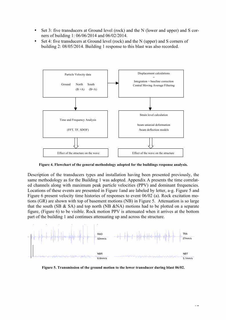
Several Matlab® routines have been developed during this work in order to derive the main time and frequency characteristics of the recorded velocity time histories and to calculate the displacements and to finally estimate the strains level within the west walls of the two build-ings. The following sections present the different results. This includes Peak Particle Velocity (PPV), Wave velocity within the structure, Principal Peak frequency, Fast Fourier Transform Analysis and Transfer Function calculations between the upper and the lower records, Single-Degree-Of-Freedom response spectra, displacement histories and strain levels. The general methodology followed in the present work is summarized in the flowchart of Figure 4 and described in the following subsections.
2 BLAST-INDUCED VIBRATIONS TIME HISTORIES
Events for which response velocity time histories were time correlated can be grouped into four clusters on the basis of the number of active transducers whose responses were time cor-related.
• Set 1: four transducers at the N (upper and lower) and S corners of the west wall of building 1: 06/27/2014; 06/30/2014; 07/07/2014; 08/05/2014
• Set 2: three transducers at Ground level (rock) and the N (upper and lower) corner of building 1: 06/09/2014 and 06/05/2014.
17
• Set 3: five transducers at Ground level (rock) and the N (lower and upper) and S cor-ners of building 1: 06/06/2014 and 06/02/2014.
• Set 4: five transducers at Ground level (rock) and the N (upper) and S corners of building 2: 08/05/2014. Building 1 response to this blast was also recorded.
Figure 4. Flowchart of the general methodology adopted for the buildings response analysis. Description of the transducers types and installation having been presented previously, the same methodology as for the Building 1 was adopted. Appendix A presents the time correlat-ed channels along with maximum peak particle velocities (PPV) and dominant frequencies. Locations of these events are presented in Figure 1and are labeled by letter, a-g. Figure 5 and Figure 6 present velocity time histories of responses to event 06/02 (a). Rock excitation mo-tions (GR) are shown with top of basement motions (NB) in Figure 5. Attenuation is so large that the south (SB & SA) and top north (NB &NA) motions had to be plotted on a separate figure, (Figure 6) to be visible. Rock motion PPV is attenuated when it arrives at the bottom part of the building 1 and continues attenuating up and across the structure.
Figure 5. Transmission of the ground motion to the lower transducer during blast 06/02.
0 0.1 0.2 0.3 0.4 0.5 0.6-50
0
50
RAD
52mm/s
Time(s)
RAD(mm/s)
0 0.1 0.2 0.3 0.4 0.5 0.6-50
0
50
TRA
27mm/s
Time(s)
TRA(mm/s)
0 0.1 0.2 0.3 0.4 0.5 0.6-50
0
50
RAD
52mm/s
Time(s)
RAD(mm/s)
0 0.1 0.2 0.3 0.4 0.5 0.6-50
0
50
TRA
27mm/s
Time(s)
TRA(mm/s)
0 0.1 0.2 0.3 0.4 0.5 0.6-50
0
50
NBR
6.6mm/s
Time(s)
NBR(mm/s)
0 0.1 0.2 0.3 0.4 0.5 0.6-50
0
50
NBT
5.1mm/s
Time(s)
NBT(mm/s)
0 0.1 0.2 0.3 0.4 0.5 0.6-50
0
50
NBR
6.6mm/s
Time(s)
NBR(mm/s)
0 0.1 0.2 0.3 0.4 0.5 0.6-50
0
50
NBT
5.1mm/s
Time(s)
NBT(mm/s)
Particle Velocity data
Ground North South (B +A) (B+A)
Time and Frequency Analysis
(FFT, TF, SDOF)
Displacement calculations =
Integration + baseline correction Central Moving Average Filtering
Strain level calculation
beam uniaxial deformation /beam deflection models
Effect of the structure on the wave Effect of the wave on the structure

18
Figure 6. Transmission of the ground motion to the lower transducer during blast 06/02.
2.1 Attenuation of peak particle velocity
Ground motions monitored in this study produced peak particle velocities (PPV’s) that atten-uate at expected rates when plotted against square root scaled distance .Table 2 gives the charge per delay and the distances from the two buildings for the eight blasts.
Peak particle velocity (PPV) and their scaled distances are compared to Oriard’s expected values in Figure 7 (Oriard, 1972). Building PPV’s fall between the upper and lower bounds of typical blasts and are well below the upper bound for confined blasts. Rock PPVs occur along Oriard’s upper bound. The higher rock motions are likely a result of the unusually small transmission distances and complete rock to rock transmission. As will be shown later, these rock to rock motions occur at unusually high frequencies and produce unusually low building response. They are rarely measured because most urban geometries only allow measurement at the street level, the lower or B level in this study.
The lower, typical PPV’s at the street level in such proximate and challenging conditions re-sult from the high drill factor (large number of holes per fractured volume) and the line drill-ing illustrated in Figure 3. The over lapping line drilling produces a slot that in most instances prevents immediate rock to rock transmission above the bottom of the slot. Typical practice advances the slot below the elevation of the bottom of the present blast holes.
0 0.1 0.2 0.3 0.4 0.5 0.6
-5
0
5 NBR
6.6mm/s
0 0.1 0.2 0.3 0.4 0.5 0.6
-5
0
5 NBT
5.1mm/s
0 0.1 0.2 0.3 0.4 0.5 0.6
-5
0
5
5.1mm/s
Time(s)
NBT(mm/s)
0 0.1 0.2 0.3 0.4 0.5 0.6
-5
0
5 NBT
5.1mm/s
0 0.1 0.2 0.3 0.4 0.5 0.6
-5
0
5 NAR
7.1mm/s
0 0.1 0.2 0.3 0.4 0.5 0.6
-5
0
5 NAT
4.4mm/s
Time(s)
NAT(mm/s)
0 0.1 0.2 0.3 0.4 0.5 0.6
-5
0
5 NAR
7.1mm/s
0 0.1 0.2 0.3 0.4 0.5 0.6
-5
0
5 NAT
4.4mm/s
Time(s)
NAT(mm/s)
0 0.1 0.2 0.3 0.4 0.5 0.6
-5
0
5 SBR
9.1mm/s
0 0.1 0.2 0.3 0.4 0.5 0.6
-5
0
5 SBT
3.8mm/s
0 0.1 0.2 0.3 0.4 0.5 0.6
-5
0
5 SBR
9.1mm/s
0 0.1 0.2 0.3 0.4 0.5 0.6
-5
0
5 SBT
3.8mm/s
0 0.1 0.2 0.3 0.4 0.5 0.6
-5
0
5 SAR
1.5mm/s
0 0.1 0.2 0.3 0.4 0.5 0.6
-5
0
5 SAT
1.7mm/s
0 0.1 0.2 0.3 0.4 0.5 0.6
-5
0
5 SAR
1.5mm/s
0 0.1 0.2 0.3 0.4 0.5 0.6
-5
0
5 SAT
1.7mm/s
0.1s

19
Figure 7. Comparison of measured square root scaled distance attenuation and Oriard’s (1972) expected values for typical practice showing the difference between rock to rock motions and those
from rock to street motions.
Table 3. Charges per delay and distances from monitored buildings for the different investigated blasts.
Blast Sym-
bol
Charge/del
ay(kg)
Vertical distance
(m)
(Scaled) Distance from Building 1
(m/kg0.5) (m)
(Scaled) Distance from Building 2
(m/kg0.5) (m)
North South North South
06/02/2014 a 2.41 9.4 (14.1) 19.8 (23.7) 35.6 (42.6) 65.5 (26.8) 40.5
06/05/2014 b 2.29 9.4 (7.3) 5.8 (35.6) 53.0 (33.1) 49.1 (17.1) 24.1
06/06/2014 c 2.41 9.4 (8.5) 9.1 (30.4) 46.3 (35.8) 54.9 (20.0) 29.6
06/09/2014 d 2.41 10.4 (7.9) 6.7 (32.1) 48.7 (34.6) 52.7 (18.9) 27.4
06/27/2014 e 2.81 13.4 (8.8) 6.0 (33.2) 54.0 (29.4) 47.4 (16.1) 23.5
06/30/2014 f 2.81 12.5 (7.5) 1.9 (33.7) 55.1 (28.2) 45.7 (14.5) 20.9
07/07/2014 g 2.81 11.0 (10.1) 12.9 (34.5) 56.7 (29.1) 47.9 (16.1) 24.7
08/05/2014 h 2.96 16.2 (11.4) 11.0 (33.6) 55.5 (29.7) 48.5 (17.2) 24.7
2.2 Ground vibration and frequency
Measurement of particle velocity time histories of rock to rock motions reveals ultra-high ex-citation frequencies. The principal peak frequency of ground motion was calculated directly from the time history because of the singular pulse excitation. Fourier frequency calculations of transient motions can be misleading unless windowed tightly around the principal pulses, which is likely to return the same frequency as that calculated directly from the time history as shown below. First, the principal pulse is detected. Then, a zero-crossing half-period of that pulse is determined and the dominant frequency is calculated as 1/(2x (½ T)) as shown in Figure 8.
Principal pulse frequencies for the radial and transverse components of all ground motion time histories recorded during the survey are compared in Table 3. These range from 250Hz to 465 Hz for the building 1 and 68 to 128 for the more distant building 2. These high princi-pal peak frequencies are one of the important unique features of this study. Implication of this ultra-high frequency motions will be discussed in the following sections.
bd
ac
h
0.1
1
10
100
1000
1 10 100 1000
PPV
(mm
/s)
Scaled distance (m/kg0.5)
CBAB DataRock Data

20
Table 4. Principal peak frequencies for rock motion time histories recorded in the two buildings
Blast Symbol Building Radial Transverse
06/02/14 a 1 435 385
06/05/14 b 1 465 341
06/06/14 c 1 333 250
06/09/14 d 1 286 266
08/05/14 h 2 68 128
3 PROPAGATION VELOCITY IN ROCK AND STRUCTURE
Propagation velocities in the rock and structure can be calculated from the differences in time correlated arrival times. Complexity of the time histories produced by close-in multi-hole blasts only allows calculation of the first arriving compressive waves. Arrival times at the N & S, lower, B, locations were employed to estimate rock propagation velocities. Arrival times at the A & B locations at the either the N or S locations were employed to calculate building propagation velocities. Figure 3 shows a simplified sketch of the geometry for a hy-pothetical position of the blast.
3.1 Rock wave velocity
Assume that the blast is initiated at time t0 and that the ground motion arrives at the northern lower point at t1 and the southern lower receiver at time t2. If the distances between the blast and these two sensor positions are respectively d1 and d2 then, the compressive wave propa-gation velocity within the rock is given by:
12
12
02
2
01
1
ttdd
Vsott
dtt
dV
−
−=
−=
−=
Based on the blast and lower N and S sensor positions, as well as on the arrival time differ-ence between the S and N records, the wave velocity could be estimated with either the R or T component records. Table 4 shows the computed values and the mean value using the three blast records. Distances account for both plan locations of the nearest boreholes and shot in-duced travel path shown in Figure 3.
3.2 Wave velocity within the structure
The compressive wave propagation velocity within the structure was derived from the transit time differences between A and B transducers and the distance between them. The transit time was computed as the difference between the wave arrival times to the lower (B) and up-per (A) sensors at Northern and Southern parts of the structure. Figure 8illustrates the time differences in arrival times with full wave forms at northern positions of the structure. Table 5 gives the propagation velocity values when traveling within the structure at the N and S corners.

21
Figure 8. Transit time estimation Case of north radial velocity wave recorded at lower and upper transducers in building 1 during
06/06/2014 event.
Table 5. Wave velocity in rock Blast # Blast date Distance to blast (m) (tS-tN) (s) Wave velocity in rock (m/s)
N S R T R T 1 6/30/2014 13.3 62.4 0.006347 0.007812 7729 6280 2 6/27/2014 10.3 66.7 0.006348 0.008301 8871 6784 3 7/7/2014 21.9 72.6 0.011718 0.0078123 4328 6492 Mean value 6976 6518
4 STRUCTURE RESPONSE TO ULTRA HIGH FREQUENCY EXCITATION FROM
CLOSE-IN BLASTING
4.1 Comparison of ground motion and structure response
Rock ground motion wave arrives with high amplitudes (up to 200 mm/s) and ultra-high fre-quency (250~500Hz). It is quickly attenuated in the structure (down to 24 mm/s in the lower, B, transducers and 21 mm/s in the upper, A, transducers) and filtered (down to 50Hz). Domi-nant frequencies at the lower, B, level are higher than that at the upper, A, level. For instance mean values of radial dominant frequencies are 108Hz and 158Hz at the lower northern and southern levels at building 1 and 72Hz and 36Hz at the upper, A, levels. The closest (06/30/2014) and the furthest (06/02/2014) blasts to the north end of building 1 produced similar dominant frequencies at both B and A levels at the north corner.
-0.02 0 0.02 0.04 0.06 0.08 0.1
-10
-5
0
5
10
Time(s)
Velo
city
(mm
/s)
NBRNAR
Δt

22
4.2 Natural frequency and damping ratio
As will be demonstrated later, these urban structures do not respond sufficiently synchro-nously to allow standard techniques for calculating dynamic response properties of the entire structure. Responses of 17 Hz components were found in several instances, but not those of the building as a whole. Some sense of dynamic structural response properties can be ob-tained by investigating amplification-deamplification of the excitation motions. The structure damping ratio was determined using two approaches using the free vibrations part of the transverse velocity time history recorded at the upper northern sensor (parallel to the short axis of the building). As mentioned by Dowding (1985, 2000), the critical damping ratio can be estimated from the decay of the free vibration using:
⎟⎟⎠
⎞⎜⎜⎝
⎛−= +
n
n
uu!! 1ln
21π
β
Where nu! and 1+nu! are successive amplitudes (Thompson, 1981). As annotated in Figure 9, the blast loading ends around 0.75s and a free vibrations period
begins until 1.8s. Two successive peaks were noted: 254.0=nu! mm/s and 381.01 =+nu! .
Therefore: =β 66.5% On the other hand, the damped natural period of the first mode of vibration, labeled T can
be read on the free vibrations plot: T=59ms So, the natural frequency is:
Hzfs 17= And the damped circular natural frequency is:
srdfpp sd /5.10621 2 ==−= πβ Where p is the undamped circular natural frequency.
Figure 9. Upper North transverse velocity time history recorded at Building 1
during blast 06/02showing free vibrations of the structure
0.6 0.8 1 1.2 1.4 1.6 1.8-3
-2
-1
0
1
2
3
0.3810.254
Time(s)
NAT(mm/s)
Free vibrations
End of blast vibrations
T

23
4.3 Amplification-deamplification
A sense of the structural dynamic response properties can be obtained from ratios of response amplification-deamplification. The greater the amplification, the closer is the building’s natu-ral frequency to the excitation frequency. These ratios can also be compared to past amplifi-cation ratios to determine the degree to which these buildings behave in similar or dissimilar fashion to those studies in the past. The most useful comparison is the amplification values observed by the US Bureau of Mines during their study of cosmetic cracking induced by blasting near residential structures (Siskind et al., 1980). To be compatible with the Siskind study, the ratios were determined from response to the principal (greatest amplitude) pulse of any blast event as illustrated in Figure 10. Given the travel time from bottom to top the re-sponse maximum was chosen as the amplitude within 0.01 sec of the principal pulse. This is not the max response; however a study with maximum response, no matter its timing with re-spect to the principal pulse, returned ratios that were similar. Three measures of amplification were examined:
• Top (A)/Rock(G): maximum velocity at the upper transducer and that at the rock lev-el.
• Bottom (B)/Rock(G): maximum velocity at the lower transducer and that at the rock level.
• Top(A)/Bottom(B): maximum velocity at the upper transducer and that at the lower. For each of these amplification factors, the two components (radial and transverse) were con-sidered. Figure 10 presents this procedure for the case of radial lower and radial ground ve-locities recorded at the northern part of building 1 during the 06/05/2014 blast event. Table 6 presents all amplification factors calculated for the 8 investigated blasts.
4.1 Mid-wall versus upper structure amplification
Basement walls are the only freely responding element in direct contact with rock. All other components respond to the attenuated building motions. Thus comparison of basement wall response to that of other elements, lower amplification (Bottom/Rock) and upper amplifica-tion (Top/Rock), is of special interest. The response of building 2 during the 08/05/2014 event provides this comparison. Basement deamplification is 0.61, which can be compared to Bottom/Rock amplification of 0.28 and Top/Rock amplification factor 0.51.
4.1 Comparison with wall and superstructure response measured by USBM
Figure 11 and Figure 12 compare amplification factors from this case and those reported by Siskind et al. (1980) for one- and two-story residential structures (homes) . Top/rock and top/bottom amplification factors obtained at the corners of the two buildings are found to the extreme right of the superstructure response (Figure12.a). In no case is there amplification, the largest ratio of 0.92. Wall/rock amplification factor for building 2 during the 08/05 event and bottom/rock amplification factors are again found on the extreme right of the wall re-sponse (Figure12.b) again there is no amplification, even for the basement wall that is in di-rect contact with the rock. However, even though it sustains high particle velocity, its relative displacement remains low because of the high excitation frequency as discussed below.

24
Figure 10. Peak velocities for radial ground motion and north lower radial component
during blast 06/05 (duration of the blast equal to 0.33s)
Table 6. Time amplification factors.
Bottom / Rock amplification Top / Rock amplification Top / Bottom amplification
Building Blast NBR/RAD NBT/TRA SBR/RAD SBT/TRA NAR/RAD NAT/TRA SAR/RAD SAT/TRA NAR/NBR NAT/NBT SAR/SBR SAT/SBT
Buil1 06/27 - - - - - - - - 0.39 0.45 0.39 0.50
Buil1 06/30 - - - - - - - - 0.68 0.92 0.19 0.09
Buil1 07/07 - - - - - - - - 0.10 0.17 0.21 0.47
Buil1 08/05 - - - - - - - - 0.26 0.38 0.11 0.36
Buil1 06/05 0.17 0.05 - - 0.09 0.04 - - 0.23 0.34 - -
Buil1 06/09 0.03 0.03 - - 0.02 0.01 - - 0.32 0.34 - -
Buil1 06/02 0.06 0.18 - - 0.05 0.10 - - 0.69 0.65 0.17 0.10
Buil1 06/06 0.05 0.007 - - 0.03 0.09 - - 0.33 0.24 0.25 0.10
Buil2 08/05 - - 0.13 0.28 - - 0.06 0.05 - - 0.51 0.19
0.05 0.1 0.15 0.2 0.25 0.3-40
-30
-20
-10
0
10
20
30
40
X: 0.09766Y: -39.37
Time(s)
RA
D (m
m/s
)
0.09 0.095 0.1 0.105-40
-30
-20
-10
0
10
20
30
40
X: 0.09766Y: -39.37
Time(s)
RADNBR

25
Figure 11. Instrumentation for USBM 1-story, 2-story residential structures and the taller urban struc-
tures of this study.
(a) Superstructure (b) Wall
Figure 12. Comparison of ratios of response to excitation observed by Siskind et al. (1980) and those from this study shows that the ultra-high frequency excitation fails to cause amplified re-
sponse.
5 PSEUDO VELOCITY RESPONSE SPECTRA DEMONSTRATE THE EXPECTAION
OF LOW DISTORTION
5.1 Filtering and SDOF Calculation
From time to time, a low frequency rider is observed in the velocity time history like that shown in Figure13 (a-upper). It persists after integration and typical baseline correction in the displacement time history and results in displacement time histories that end with a per-manent offset that cannot be true. In addition the rider produces an unusual response spec-trum as shown by the thin lined spectrum in Figure13 (b) In this study, these low frequency riders were filtered with a 200 point window central moving average filter as shown in Figure13 (a-lower) to return a velocity and displacement time history that oscillates about zero. While many explanations have been advanced for the rider, there is as yet no universally ac-cepted explanation. This particular case is enlightening, as it rules out one possibility, a de-layed gas pressure pulse. As shown in Figure14, the rock motions (G) do not contain this low
0
2
4
6
8
5 50 500
Amplificatio
nFactor
GroundVibrationFrequency(Hz)
1story(USBM)
2stories(USBM)
TOP/ROCK
TOP/BOTTOM
0
2
4
6
8
5 50 500
Amplificatio
nFactor
GroundVibrationFrequency(Hz)
1story(USBM)
2stories(USBM)
BOTTOM/ROCK
WALL/ROCKBUIL2
W

26
frequency motion, while those measured at building’s street level, B1 (a) do. Therefore it cannot be a result of a delayed gas pressure pulse, which if it existed, would be evident in the rock motions. The possibility that the rider is the building’s fundamental frequency response, is also unlikely as it occurs too early in the time history, was not observed at the south end and there was no free response at this low frequency after excitation ceased. Pseudo velocity response spectra were calculated with two routines; NUVIB2 and Matlab. NUVIB2 (Chok t al., 2003) is software developed at the Department of Civil Engineering of Northwestern University to process velocity time histories with provisions for filtering, and baseline correction. The Matlab routine was developed by (Papazafeiropoulos, 2014) which is based on the General Single Step Single Solve (GSSSS) family of algorithms published by (Zou and Temma, 2004). These algorithms are employed for direct time integration of the various SDOF oscillators.
(a) Measured and corrected velocity time histories (b) Measured and corrected response spectra
Figure 13. Drift correction and response spectrum calculation (case of NBT, blast 06/02/2014)
Figure 14. Radial rock motion time history (case of NG, blast 06/02/2014)
0 0.1 0.2 0.3 0.4 0.5 0.6-5
0
5
5.1mm/s
Time(s)
NBT(
mm
/s)
0 0.1 0.2 0.3 0.4 0.5 0.6-5
0
5
5.9mm/s
Time(s)
Corre
cted
NBT
(mm
/s)
0 0.1 0.2 0.3 0.4 0.5 0.6-5
0
5
4.4mm/s
Time(s)
NAT(mm/s)
0 0.1 0.2 0.3 0.4 0.5 0.6-5
0
5
5.1mm/s
Time(s)
NBT(mm/s)
100 101 102 10310-1
100
101
102
Fn (Hz)
PSV(m
m/s
)
Pseudo Velocity Spectrum (mm/s)
NBTCor. NBT
0 0.1 0.2 0.3 0.4 0.5 0.6-50
-40
-30
-20
-10
0
10
20
30
40
50
52mm/s
Time(s)
RAD(mm/s)

27
5.2 Comparison with MS Excel 200-central moving average filtering The results of such a Matlab procedure was compared to those of performing a simple Cen-tral Moving Average of the velocity time history using Excel software. Figure 15 gives the raw measured NBT velocity time history as recorded during 06/02 event and the central mov-ing average using 200 point window. This figure shows the drift phenomenon that should be removed from the raw data. Figure 16 and Figure 17 give the results of data processing using respectively the Excel central average moving filter and the developed Matlab procedure. The Peak Particle Velocities obtained from these two methods are respectively 5.97 mm/s and 5.94 mm/s. This so small difference is due to error in calculations as the Matlab procedure uses integration of raw velocity data (to obtain displacement) and then derivation to re-compute the corrected time history velocity.
Figure 15. Raw NBT velocity time history as recorded during 06/02 blast event and 200-central moving
average.
Figure 16. Drift correction using 200-central moving average in MS Excel
(case of NBT velocity time history as recorded during 06/02 blast event)
Figure 17. Drift correction using 200-central moving average in Matlab
(case of NBT velocity time history as recorded during 06/02 blast event).
-6
-4
-2
0
2
4
6
-0.3 -0.2 -0.1 0 0.1 0.2 0.3 0.4 0.5 0.6 0.7
Velocity(m
m/s)
Time(s)
CMAF(mm/s)
RawNBT(mm/s)
-6
-4
-2
0
2
4
6
-0.3 -0.2 -0.1 0 0.1 0.2 0.3 0.4 0.5 0.6 0.7
Velocity(m
m/s)
Time(s)
-6
-4
-2
0
2
4
6
-0.3 -0.2 -0.1 0 0.1 0.2 0.3 0.4 0.5 0.6 0.7
Velocity(m
m/s)
Time(s)

28
5.3 Comparison with tunnel and quarrying blasts Considerations of energy and mass show that response of large, urban structures to ultra-high frequency excitation is likely to be lower than that predicted by standard response spectrum analysis. First consider single degree of freedom (SDOF) pseudo velocity response with 5% damping of the 06/02 event compared to shown with that from a large, distant quarry (B) and close tunnel (A) blast shown in Figure 18. Details of this calculation are described in Appen-dix B. Spectrum A was developed from ground motions recorded 12m (38ft) away from a 0 to 9 ms delayed tunnel blast with a maximum charge in any single delay of 1.7 kg (3.8lb). Spectrum B was developed from the ground motions recorded 72m (220ft) away from a sin-gle 91 kg (200lb) charge detonated in a typical bench blast hole in a limestone quarry. The quarry blast generated a peak radial particle velocity of 43 mm/s (1.7 in/s) and the tunnel blast generated a peak radial particle velocity of 61 mm/s (2.39 in/s) (Dowding, 2000). The 06/02/2014 blast generated a radial peak particle velocity of 51 mm/s in the rock from a 2.4 kg blast some 9+ m distant.
Figure 18. Comparison of response spectra of ground motions from close-in blast event 06/02 and a low frequency quarry blast (Q) and a near-by tunnel blast (T).
Even though the peak particle velocities are similar, standard response spectrum analysis pre-dicts that a single story, 10Hz structure will sustain a response velocity 60 and 6 larger for the quarry and tunnel blasts. Since the pseudo velocity is proportional to relative displacement for structures with the same natural frequency ( 10 Hz in this case), the 06/02 event would be expected to induce far less relative displacement, strain, and cosmetic cracking to a typical single story residential structure. Now consider that these particular urban structures are far more massive because of their size and masonry construction. Their super structures can be expected to have periods, T, of 1/10 sec per story, where a five story structure would have a
100 101 102 10310-1
100
101
102
103
Fn (Hz)
PSV(m
m/s
)
Tunnel (T)Quarry (Q)
GRGT

29
natural frequency (1/T) of 1/ (5*0.1) = 2 Hz. The 2 Hz response to the 06/02 event is 1/5th that of the 10 Hz response and an urban structure would likely sustain 1/5th the relative dis-placement strain and cosmetic cracking. Response of the urban structure is likely to be even less than predicted by SDOF analysis. SDOF analysis carries with it an implicit assumption that the entire building is AND can be entirely excited synchronously. First consider synchronous excitation. These urban structures have a larger foot print (65 x 15 m ) compared to a residence (8 x 10 m) and are excited by motions with pulses ( = ½ a wave length) that are only 10 m (= c/f = 6000 m/s/300 Hz). The distance from the north to the south of building 1 is 3 wave lengths. The same pulse cannot excite the entire structure synchronously. Now consider the mass to energy ratio. A structure with a natural frequency of 2 Hz that is 4 time stiffer than a 10 Hz structure would be some 100 times more massive if its natural frequency could be estimated as the square root of the stiffness divided be the mass. Now consider the energy of the excitation pulses. If it is as-sumed that the energy of the excitation is proportional to the peak particle velocity divided by peak acceleration (Sucuoglu and Nurtug, 1995) or 1/f of a single principal pulse event with the same displacement, then a 300 Hz excitation is some 100 times less energetic than a 30 Hz event. Thus the energy to mass ratio of the close-in rock blast excitation of an urban struc-ture is 1/10,000 that of a quarry blast excitation of a residential structure. Thus there are two reasons to suspect that close in blast perturbation of a large urban structure will produce less distortion than a SDOF analysis: it is not excited synchronously and the energy to mass ratio is smaller than associated with observations of cosmetic cracking.
6 COMPARISON OF TIME CORRELATED TIME HISTORIES ILLUSTRATES WAVE
TRANSMISSION
Time correlated comparison of rock excitation and building response motions demonstrates that the buildings do not respond synchronously as a unit. Table 7 presents maximum veloci-ty amplitudes and arrival times of the blast-induced response at the northern and southern transducer strings of all events. To more clearly illustrate details of building response, veloci-ty time histories from one event are plotted in a common amplitude scale in their relative po-sitions in both time and space in Error! Reference source not found.. Differences in times of arrival are illustrated by the arrows. Differences in amplitude are illustrated by differences in size. Arrival times are delayed by some 60 milliseconds (ms). This time difference is large enough to encompass some 3 separate excitation pulses as shown by comparison of differ-ences in arrival times and the excitation motions at the bottom of the figure. Amplitudes and dominant frequencies decline both upward and across (north to south) the structure. Structure response amplitudes and dominant frequencies decline by factors of 5 at the north, which is closest to the blast. Dominant rock excitation frequency is 333 Hz and the dominant response frequency is only 60 Hz. These responses: large deamplification and significant delays in building response are more reflective of wave transmission than synchronous dynamic re-sponse.

30
Table 7. Amplitudes and time arrival at northern upper and southern upper part for the transverse com-ponent.
Building Blast Symbol A(NAT) t(NAT) A(SAT) t(SAT) A(S)/A(N) Dt
(mm/s) (ms) (mm/s) (ms) % (ms)
1 06/27/2014 e 6.1 7.81 0.9 83.98 14.8 76.2
1 06/30/2014 f 19.8 6.34 1.7 58.11 8.6 51.8
1 07/07/2014 g 8.5 12.7 1.1 75.2 12.9 62.5
1 08/05/2014 h 4.1 7.81 1.1 35.63 26.8 27.8
1 06/02/2014 a 4.4 -22.46 1.7 31.74 38.6 54.2
1 06/06/2014 c 10.2 3.42 1 31.25 9.8 27.8
2 08/05/2014 h 8.3 -66.41 2 -40.53 24.1 25.9
Building Blast Symbol A(NBT) t(NBT) A(NAT) t(NAT) A(A)/A(B) Dt
(mm/s) (ms) (mm/s) (ms) % (ms)
1 06/27/2014 e 10.8 -4.4 6.1 7.81 56.5 12.2
1 06/30/2014 f 17.3 -3.9 19.8 6.34 114.5 10.2
1 07/07/2014 g 22.9 -3.4 8.5 12.7 37.1 16.1
1 08/05/2014 h 6.6 -4.8 4.1 7.81 62.1 12.6
1 06/02/2014 a 5.1 -32.7 4.4 -22.46 86.3 10.2
1 06/06/2014 c 10.8 -5.4 10.2 3.42 94.4 8.8
2 08/05/2014 h - - 8.3 -66.41 - -
7 CONCLUSION
Measurements of multiple positions, time correlated response of two urban buildings to ultra-high frequency excitation allow the following observations to be made. These observations are based upon bidirectional horizontal velocity responses at ten positions during eight blast events, which provided over 70 time histories for analysis.
• Close-in blasting with rock transmission imposes isolated, ultra-high frequency exci-tation pulses with a short duration.
• First arrival propagation velocities are high as expected for this rock • Excitation motions attenuate as expected from scaled distance relations • The structures respond predominantly in a wave transmission mode where there is no-
ticeable difference in time, frequency, and amplitude of motions measured at the ex-treme top corners of the structure.
• Excitation motions along the base are not the same; they differ significantly in both time, frequency, and amplitude.
• Excitation frequencies are so much larger than the natural frequencies of the struc-tures and components that the excitation motions were deamplified for all events.

31
Figure 19. Spatial variation of time correlated transverse building1 velocity during blast 06/02/2014. Shown are differences in 1) times of arrival by arrows 2) amplitude by same scale (except rock motion is
at 1/3 scale) 3) dominant frequencies by wave train time histories.
0 0.05 0.1 0.15 0.2 0.25 0.3 0.35
-5
0
5
0 0.05 0.1 0.15 0.2 0.25 0.3 0.35
-5
0
5
00.05
0.1
0.15
0.2
0.25
0.3
0.35
-505
00.05
0.1
0.15
0.2
0.25
0.3
0.35
-505
0 0.05 0.1 0.15 0.2 0.25 0.3 0.35
-5
0
5
0 0.05 0.1 0.15 0.2 0.25 0.3 0.35
-5
0
5
00.05
0.1
0.15
0.2
0.25
0.3
0.35
-505
00.05
0.1
0.15
0.2
0.25
0.3
0.35
-505
0 0.05 0.1 0.15 0.2 0.25 0.3 0.35
-5
0
5
0 0.05 0.1 0.15 0.2 0.25 0.3 0.35
-5
0
5
0 0.1 0.2 0.3 0.4 0.5 0.6
-5
0
5
5.1mm/s
Time(s)
NBT(mm/s)
0 0.1 0.2 0.3 0.4 0.5 0.6
-5
0
5
NA NB NG
SA SB
NA SA

32
Chapter 3. Close-in blast induced strains
1 GROUND MOTION ENVIRONMENT
Ground motions monitored in this study produced peak particle velocities (PPV’s) that atten-uate at expected rates when plotted against square root scaled distance. These PPV’s and their scaled distances are compared to Oriard’s expected values in Figure 7 (Oriard, 1972). Street level (B) PPV’s fall between the upper and lower bounds of typical blasts and are well below the upper bound for confined blasts. Rock (G) PPV’s occur along Oriard’s upper bound. The higher rock motions are likely a result of the unusually small transmission distances and complete rock to rock transmission. These rock to rock motions occur at unusually high fre-quencies (300 to 500 Hz) and produce unusually low building response as shown by the re-sponse spectra of the rock motions in Figure 18. Rock motions are rarely measured in urban blasting because most immediately adjacent urban excavations only allow measurement at the street level, the lower or B level in this study, because rock is inaccessible at the begin-ning and changes elevation with the adjacent excavation. There are many possible explanations for the lower PPV’s on the building at the street level. Large mismatches between response and excitation frequencies (0.5 and 500 Hz) results in very low velocity response as shown in the response spectrum in Figure 18. The small energy in a 500 Hz pulse is not sufficient to excite these relatively massive (compared to a one story suburban residence) structures. The impulse is so small (due to its infinitesimally small dura-tion) that it imparts little change in the momentum of the structure. High attenuation, and change in phase of excitation motions along the structure creates high damping overall and low response.
1.1 Integration of velocity time history
As described in the introduction, strains associated with the fundamental, dominant, or first mode of response can be calculated from time correlated displacements, which were devel-oped by integrating the velocity time histories. Before calculation of strains, the velocity time histories were corrected for baseline irregularities. An example of the four steps in this cor-rection process is shown in Figure 20. First, the velocity time history (Figure 20.a) is baseline corrected. Linear and second order polynomial baseline corrections were tested as shown in Figure 20.b, As can be seen the polynomial correction did not remove the low frequency (~ 2

33
Hz artifact) that is not in the original velocity time history. It was removed by subtracting the 200 point central-moving–average shown in Figure 20.c to produce the displacement time history that oscillates about 0 as shown in Figure 20.d.
Figure 20. Displacements calculation by drift correction and 200 point central-moving-average filtering
(case of SBT recording at Building 2): (a) (top)Velocity recording, (b) Displacement after linear and second order polynomial baseline correction, (c) 200 point central-moving-average filtering of the second
order baseline correction displacement, (d) (bottom) Final displacement.
1.2 Differential displacement calculation
Prior to the calculation of strains, the differential structure motions were computed from the difference between displacements at the upper, A, and lower, B, transducer positions. Rela-tive displacements, δ, were calculated in both the radial (parallel to the plane of the west wall) and in transverse directions. Differential displacements in these two directions allowed calculation of in-plane shear and tensile strain as well as out-of-plane bending strains. Since the motions were time correlated, the differential displacements are most simply calculated as the difference in displacements at the two transducers at the same time. The high rate of sam-pling, 2048 samples per second, allows precise time correlation. Calculation of differential displacement can be subdivided into the following steps that are il-lustrated in Figure 21 for event 06/06. Velocity time histories are first integrated using the procedure described in the previous section to obtain displacement time histories. Then the differential displacement is found by simple subtraction of the two displacements (at A & B) at the same time. These differential displacements are then searched for the largest. Plots of the transverse velocities recorded at upper and lower transducers of Building 1, as well as corresponding displacements and differential displacements time histories for the 06/06 event are shown in Figure 21. Table of Appendix A compares the maximum calculated differential displacements between measurement points and PPV’s induced by all eight events. The maximum recorded whole or super-structure differential displacement was 334.4µm between the rock (G) and lower (B-street) levels at the north corner of building 1 during the 06/09 event. The maximum calculat-
LinearPolynomial
LinearPolynomial
Data200 CMA Filter
-0.1 0 0.1 0.2 0.3 0.4 0.5 0.6 0.7Time(s)
Data200 CMA Filter
-0.1 0 0.1 0.2 0.3 0.4 0.5 0.6 0.7Time(s)

34
ed differential displacement between bottom (B) and top (A) was 178.7 µm at the north cor-ner of the building 1 during the 07/07 event.
Appendix B contains all velocity and displacement time histories for all events.
Figure 21. Differential transverse displacements between the top and bottom north corners of building 1
case of the 06/06 event: a) top two time histories–velocities at top (NAT) and bottom (NBT); b) middle two time histories – displacements at top and bottom and c) bottom time history – difference between top
and bottom displacements.
2 STRAIN CALCULATIONS
2.1 Procedure for calculating strains
Two types of strain can be calculated: a) distortion parallel the plane of the wall and b) distor-tion perpendicular to the plane of the wall (Dowding, 2000). First consider distortion parallel to the plane of a building wall, which produces shear strains that can be calculated as:
Lδ
γ =
(1)
where L is the wall or building height and δ is the distortion or difference of displacement between the top and bottom of the wall in a direction parallel to the plane of the wall . This shear strain can be translated into tensile strains, εt, as follows:
ϕϕδ
ε cossinLt = ; )/arctan( WH=ϕ (2)
where H is the wall height (or in this case the vertical distance between transducer loca-tion) and W is the width (not thickness) of the wall or building face on which the transducers are located. The H and W’s employed in these calculations are visible in Figure 2 and are enumerated in a footnote in the Appendix A table.
NAT - 10mm/s
NBT - 11mm/s
NAT - 10mm/s
NBT - 11mm/s
NAT - 0.052mm
NBT - 0.036mm
NAT - 0.052mm
NBT - 0.036mm
0 0.1 0.2 0.3 0.4 0.5 0.6Time(s)
Dif - 0.058mm
0 0.1 0.2 0.3 0.4 0.5 0.6 0.7 0.8 0.9 10
0.5
1

35
Now consider distortion in a direction perpendicular to the plane of the wall, which produces bending strains in the wall. A beam deflection model, which assumes a “fixed-fixed” end condition, was used to calculate the strain from the relative displacementδ :
26Lcδ
ε =
(3)
where c is the distance from neutral axis to most extreme fiber, taken here as half the wall thickness and L is the length of the beam or in this case the height of the wall or distance be-tween the two transducers, H. For calculations in this study, the walls were assumed to be 18 mm (7 in) thick. The fixed-fixed condition was assumed as it gives the highest strain calcula-tion (most distorted mode shape)
5.2 Induced Strains
Appendix A enumerates and compares all the PPV’s and maximum strains induced in the two buildings by the eight blast events. As described above these strains were calculated from the differential displacements that are also compared in this table. Maximum and minimum glob-al (A-B) in plane shear strains were 12.0 and 0.3µ-strains respectively. Corresponding maxi-mum in-plane tensile strain calculated was 4.8µ-strains. The blast induced strains are low despite high excitation particle velocities. They vary from blast to blast as would be expected. All of the strains are smaller to the south in building 1, which is some 60 m south of the blasts located at the north corner as shown in Figure 1. This consistent difference results (A-B) from the attenuation of the ground motions along the base of the structure. North to south declination on strain ranges from 75% to 97% for the radial strains and from 70% to 96% for the transverse strains.
Basement response is more complex. While shear and tensile strains in the basement can be calculated from the differential displacements, they are not reflective of whole body distor-tion. They are calculated from differences in displacement time histories which are differ-ences in amplitude of waves propagating through the structure. First consider shear strains. The street level floor is not free to move laterally as the floors above because the basement walls supporting it are restrained from lateral movement by the soil surrounding the basement walls. Thus there can be no free response of the walls or free inter-story “drift” between the basement floor and the street level floor without interaction with the surrounding soil and in-frastructure. In other words the basement walls and first story cannot be treated as single de-gree of freedom systems defined by their mass stiffness and damping. Calculated basement strains between the rock (G) and lower building transducers (B) tabulat-ed in Appendix A do not reflect the strains that would be calculated from inter-story drift for the freely responding upper floors. Even though they were calculated with equations in Sec-tion 5.1, the underlying assumption of synchronous, free inter-story drift, is not valid because of the restraint provided by the surrounding soil. Calculated basement strains are presented only to show the degree to which the differential displacements decline in the above ground section of the building. The ratio between the upper building shear strains (A-B) and the basement shear strains (B-G) strains ranged from 10% to 72% in the transverse direction and 11% to 82% for the radial shear strains. This declination s expected as the lower portion of the building absorbs the vibratory energy first. The greatest declinations of strains above the

36
basement level occurred with rock motions at the north end of building 1 that exceeded75 mm/s (3 ips). The largest excitation motion was some 200 mm/s (8 ips). These high PPVs oc-curred at dominant frequencies of greater than 300 Hz.
There is one basement location where there can be response without interaction with the sur-rounding soil and below-ground infrastructure: out of plane bending of the west basement wall adjacent to the excavation. Response of the basement mid-wall (W) transducer on build-ing 2 to the 08/05 event discussed below demonstrates the extent to which the basement wall responds in this direction
2.3 Basement Wall response at building 2
Of special interest is the out plane response of a wall, which cannot be calculated with corner motions. This location is of particular interest as it is the only wall that 1) can respond freely without interaction with the surrounding soil and 2) is distorted directly by rock motions. Walls separating above-ground floors are excited by motions transmitted by the building, which have been shown to decline significantly with distance from the blast location and ele-vation.
Displacements of the mid wall (W) transducer at building 2 can be employed to calculate ten-sile bending strains. The out of plane, beam bending model is employed with time correlated displacements measured in the rock (G) and at the street level (B).The L distances needed for this calculation were those shown in Figure 2. For the particular case, three values of the rela-tive transverse displacements, δ , were used: either a) SBT-W, or b) W-GT components, or c) Wall- average SBT and GT as shown in Figure 22. Differential displacements between the transverse rock (GT) and mid-wall (W) motions are shown in Figure 23(a) in relation to the velocity and displacement time histories.
The out of plane response basement wall response is not large. The PPV of the mid-wall was 7.1 with a rock excitation of 5. 2 mm/s at 140 Hz. Calculated tensile bending strains of 0.6 to 1.45 µ-strains are similar to the tensile strains calculated from the in-plane shear strains in walls above the street level. They are small compared to the stains that are necessary to cos-metically crack brick mortar and weak wall covering (300 to 500 µ-strains) (Alan and Adrian, 2002; Dowding, 2000).
Figure 22. Displacement in the bottom southern part of the wall in Building 2 (W: Mid-wall, SBT: south lower, GRT: transverse ground motion).
SBTT
WT
GRT
Initial position of the wall
.Rock
B.
W

37
Figure 23. Differential displacements calculation
(case of rock and mid-wall recordings at Building 2 during blast 08/05/2014): (a) and (b) Velocity re-cordings, (c) and (d) Displacements after second order polynomial baseline correction, (e) Final differen-
tial displacement.
2.4 Comparison with ACM surveillance
Comparison of differential displacements and strains from this case study with those from au-tonomous crack monitoring (ACM) will allow an assessment of the level of dynamic distor-tion relative to that induced by weather effects. While this comparison is not as direct as measurement of the weather effects in these urban structures, it does provide a measure of the significance of the differential displacements and strains induced by urban blasting. This comparison is made through use of the Table 2 which presents crack response and strains and differential displacements induced by quarry blasting near suburban, one to two story resi-dential structures as well as strains and differential displacements induced in this study. Comparisons of the strain columns in Table 2 show that close-in blasting induces less distor-tion and strain (< 1.5 to 12 µ-strains) in urban structures than does typical quarry blasting near residential structures (0.3 to 280 µ-strains). Furthermore comparison of the blast in-duced crack response (3rd column from the right) with that induced by weather effects (last two columns on right) shows that these larger blast induced strains in residential structures fail to induce crack response that is greater than that induced by weather effects. Thus by ex-tension, if the urban structures are as responsive to weather effects as the suburban residential structures, than crack responses induced by close-in blasting are small compared to those in-duced by weather effects.
Further perspective for the significance of strains of less than 12 µ-strains is provided by strains necessary to crack wall covering material such as drywall (plasterboard). Strains nec-
GT - 5.2mm/s
W(T) - 7.1mm/s
GT - 5.2mm/s
W(T) - 7.1mm/s
GT - 0.0076mm
W(T) - 0.019mm
GT - 0.0076mm
W(T) - 0.019mm
0 0.1 0.2 0.3 0.4 0.5 0.6Time(s)
Dif - 0.018mm

38
essary for cracking are on the order of 300 to 500(Alan and Adrian, 2002; Dowding, 2000; AS3600, 1998).
Table 8. Differential displacements and strain levels in previous ACM and non ACM studies (d: absolute distance; f:peak frequency; Dif: Maximum differential displacement; τ: Maximum shear
strain; σ: Maximum in-plane tensile strain. Reference Construction Blast
type d
(m) Charge
(kg) PPV
(mm/s) f
(Hz) Dif
(µm) H
(m)
τ (µstrain
s)
σ (µstrains)
Crack disp./blast
(µm)
Crack disp./daily
(µm)
Crack disp./front
(µm)
Louis (2000) Book House Quarry - - 19 - 8.9 2.8 3.2 - 10 6 25 One-story, concrete masonry Quarry - - 3.3 - 7.0 2.8 2.5 - 43 58 21
McKenna (2002)
Double-wide trailer Mine 438 277.5 8.1 - 150.2 2.1 71.5 - 0.9 24.4 16.2 Adobebrick ranch house Mine 1506 4350 4 - 49.3 4.8 10.2 - 4.2 20.1 9
Concrete block basement wall Mine 315 68 5.8 - 19.0 2.4 7.9 - 0.3 12.5 -
Distressedwood-framed house Mine 635 476 7.1 - 2.3 6.1 0.3 - 13.6 53 10.9
Stone-faced, con-crete block Quarry - - 4.5 - 11.7 2.9 4 - 5 47 20.7
Alan and Adrian (2002)
Conventional brick veneer Mine 450 1300 20.8 10 - - 282.4 47.8 84 2200
(rainfall) -
Single and double storey Mine 700 800 2.37 10 - - 47.5 6.6 270 - -
Aimone and Dowding (2005)
Brick structure Quarry 335 73.4 2.74 8.0 236.2 5 47 21 6.8 38.1 4.5
Aimone and Rosenhaim (2006)
Concrete masonry brick structure Quarry 825 42.6 1.85 28.4 17.0 2.8 4.6 2.48 2.9 137.8 1386
Two-structure wood frame Quarry 825 42.6 1.85 28.4 24.4 2.3 12.4 6.2 7.4 510 30505
Rosenhaim et al. (2005)
Wood frame house -stucco exterior
Pre-split 293 87.9 9.27 5.2 496.1 3.6 135.6 67.4 73.9 300 410
Abeel (2012) Five-story masonry load bearing
Close-in - 3.6 62 >150 - - 12.0 - - - -
Present study
Building 1, d, NT(A-B)
Close-in 6.7 2.41 200.4 500 70 11.6 2.5 - - - -
Building 1, b, NT(A-B)
Close- in 1.9 2.81 128.8 500 54 11.6 4.7 4.8 - - -
Building 2, h, GT(B-G)
Close-in 24.7 2.96 5.2 143 19.1 15.8 1.4 - - - -
Maximum differential displacements induced in these urban structures by ultra-high frequen-cy ground motion are also compared to those measured in residential structures in Table 2. Responses of the suburban one to two story residential structures were induced by typical quarry blasting during autonomous crack monitoring (ACM) studies (Dowding and McKen-na, 2005). The maximum differential displacement observed in that 2005 study was 150 µm for case T. Even in case T the weather induced crack displacements (last two columns in Ta-ble 2) were more than 15 times greater than induced by blasting (3rd column from the right)
2.5 Comparison with previous studies of tall structure response in urban close-in
blasting
Strains measured in this study are lower than those observed in similar tall urban structures by Aimone et al (2014). Figure 24 compares data from this case with that of others by com-paring calculated strains with peak ground displacement up to 0.1 mm. Aimone data are pre-sented as the insert to Figure 24, with both the figure and insert possessing the same range of strains (up to 7 µ-strains). While this study included situations with greater peak ground dis-placement, smaller strains were induced as some of the data fall outside the lower limit curve (A) and upper limit bound (B). The upper bound of all strains vs peak ground displacement as reported by Aimone et al. (2014) is not exceeded.

39
Figure 24. Strains at the top and bottom of buildings versus peak ground displacement. Comparison with Aimone et al. (2014)
3 STRAINS VERSUS PEAK PARTICLE VELOCITIES
Figure 25 to Figure 28 shows the variation of the maximum differential displacement and the resulting shear strains versus the Peak Particle Velocity (PPV) and the ratio PPV over princi-pal pulse frequency. These figures confirm an increasing trend of strains within the structure when the generated PPV or PPV/f ratio increases.
0
1
2
3
4
5
6
7
0 0.05 0.1 0.15 0.2 0.25 0.3 0.35 0.4
Strains(
µ-strains)
PeakGroundDisplacement(mm)
Shear(Top) Tension
AB
Aimone et al. (2014)

40
Figure 25. Variation of Maximum Differential Displacement versus the PPV of ground/street level mo-
tion.
Figure 26. Variation of Shear strains versus the PPV of ground/street level motion.
0
50
100
150
200
250
300
350
400
0 50 100 150 200 250
Maxim
umDifferen
tialD
isplacemen
t(µm
)
PPV(mm/s)
0
10
20
30
40
50
60
70
0 50 100 150 200 250
ShearS
trains(µ
strains)
PPV(mm/s)

41
Figure 27. Variation of Maximum Differential Displacement versus the PPV/f of ground/street level mo-
tion.
Figure 28. Variation of Shear strains versus the PPV/f of ground/street level motion.
4 SINGLE-DEGREE-OF-FREEDOM RESPONSE SPECTRA
Comparison of the pseudo velocity response spectrum of the 500 Hz dominant frequency rock (G) motions from the 06/02 event is compared with that from a distant quarry (Q) and
0
50
100
150
200
250
300
350
400
0.000 0.050 0.100 0.150 0.200 0.250 0.300 0.350 0.400 0.450
Maxim
umDifferen
tialdisp
alcemen
t(µm
)
PPV/f(mm)
0
10
20
30
40
50
60
70
0.000 0.050 0.100 0.150 0.200 0.250 0.300 0.350 0.400 0.450
ShearS
trains(µ
strains)
PPV/f(mm)

42
close tunnel (T) blast in Figure 18. Spectrum T was developed from ground motions recorded 12m (38ft) away from a 0 to 9 ms delayed tunnel blast with a maximum charge in any single delay of 1.7 kg (3.8lb). Spectrum Q was developed from the ground motions recorded 72m (220ft) away from a single 91 kg (200lb) charge detonated in a typical bench blast hole in a limestone quarry. The quarry blast generated a peak radial particle velocity of 43 mm/s (1.7 in/s) and the tunnel blast generated a peak radial particle velocity of 61 mm/s (2.39 in/s) (Dowding, 2000). The 06/02 blast generated a radial peak particle velocity of 51 mm/s in the rock from a 2.4 kg blast some 9+ m distant.
Even though the peak particle velocities are similar, standard pseudo-velocity response spec-trum analysis in Figure 38 predicts that a single story, 10Hz structure or component will sus-tain a response velocity 60 and 6 times larger for the quarry and tunnel blasts than for the 06/02 event. Since the pseudo velocity is proportional to relative displacement for structures with the same natural frequency (10 Hz in this case), the 06/02 event would be expected to induce far less potential relative displacement, strain, and cosmetic cracking than induced in a typical single story residential structure or 10 Hz component. Furthermore, since the larger urban structures, have lower fundamental frequencies (2 to 3 Hz) expected superstructure rel-ative displacements would be 3 to 5 times lower than 10 Hz structures.
Although the SDOF response spectrum in Figure 38 shows that the relative displacements will be low, additional comparisons show that relative displacements calculated with the SDOF model (SDOF) do not match those calculated from the measured velocity time histo-ries (Diff). For instance, while it is not always true, use of rock motions to calculate SDOF relative displacements will more closely match those measured DIFF relative displacements. Use of street level motions with the SDOF model tended to yield relative displacements that were smaller than measured, Diff. However relative displacements and shear strain calculated with from velocity time histories were still small in absolute sense.
4.1 Displacement estimated from SDOF response spectrum SDOF model response spectrum corresponding to the bottom (rock or street level, B) velocity time histories was used in order to estimate the displacement and compared to the maximum differential displacement computed from integration of the velocity time histories. The procedure adopted for the estimation of SDOF spectrum based displacement is as fol-lows: 1. For each frequency data between 2.5 Hz and 16Hz, the displacement is computed as:
i
ii f
Vπ
δ2
= where Vi is the Pseudo velocity corresponding to frequency fi
2. The SDOF based displacement is defined as the average value on all N frequencies of the considered range:
∑=
=N
iiN
SDOF1
1)( δδ
For instance, Figure 29 to Figure 32 show the raw velocity time history (a), the corresponding displacement time history (b), the corresponding response spectrum (c) and the SDOF based displacement variation between 2.5 Hz and 16Hz (d) respectively for the NBT and NBR (blast 08/05, building 1) and NBT (blast 07/07 and blast 06/02, building 1).

43
In the present work, it has been decided to use the average value which is thought to be the most representative value of displacement over the range of frequencies that represent most likely the natural behavior of the building.
(a)Velocitytimehistory (b)Displacementtimehistory
(c)SDOFspectrum (d)Displacementbetween2.5Hzand16Hz
Figure 29. SDOF displacement calculation for NBR time history recorded during 08/05 event in building 1.
0 0.1 0.2 0.3 0.4 0.5 0.6
-6
-4
-2
0
2
4
6
Time(s)
NBR(mm/s)
0 0.1 0.2 0.3 0.4 0.5 0.6
-0.01
-0.008
-0.006
-0.004
-0.002
0
0.002
0.004
0.006
0.008
0.01
Time(s)
NB
R d
isp.
(mm
)
100 101 102 10310-2
10-1
100
101
102
Fn (Hz)
PSV (m
m/s
)
4 6 8 10 12 140.008
0.01
0.012
0.014
0.016
0.018
0.02
0.022
Fn (Hz)
SDO
F di
spl.(
mm
)
0.011mm

44
(a)Velocitytimehistory (b)Displacementtimehistory
(c)SDOFspectrum (d)Displacementbetween2.5Hzand16Hz
Figure 30. SDOF displacement calculation for NBT time history recorded during 08/05 event in building 1.
0 0.1 0.2 0.3 0.4 0.5 0.6
-5
-4
-3
-2
-1
0
1
2
3
4
5
Time(s)
NBT(mm/s)
0 0.1 0.2 0.3 0.4 0.5 0.6
-0.015
-0.01
-0.005
0
0.005
0.01
0.015
Time(s)
NB
T di
sp.(m
m)
100 101 102 10310-1
100
101
102
Fn (Hz)
PSV (m
m/s
)
4 6 8 10 12 140.01
0.015
0.02
0.025
0.03
0.035
Fn (Hz)
SDO
F di
spl.(
mm
)0.025mm

45
(a)Velocitytimehistory (b)Displacementtimehistory
(c)SDOFspectrum (d)Displacementbetween2.5Hzand16HzFigure 31. SDOF displacement calculation for NBR time history recorded during 06/02 event in building
1.
0 0.1 0.2 0.3 0.4 0.5 0.6
-6
-4
-2
0
2
4
6
Time(s)
NBR(mm/s)
0 0.1 0.2 0.3 0.4 0.5 0.6
-0.01
-0.005
0
0.005
0.01
Time(s)
NB
R d
isp.
(mm
)
100 101 102 10310-2
10-1
100
101
102
Fn (Hz)
PSV (m
m/s
)
4 6 8 10 12 140.01
0.012
0.014
0.016
0.018
0.02
0.022
0.024
0.026
Fn (Hz)
SDO
F di
spl.(
mm
)
0.015mm

46
(a)Velocitytimehistory (b)Displacementtimehistory
(c)SDOFspectrum (d)Displacementbetween2.5Hzand16HzFigure 32. SDOF displacement calculation for NBT time history recorded during 06/02 event in building
1.
4.2 SDOF displacement versus PPV/freq and PPV Figure 33 shows the variation of the so computed SDOF displacement versus the ratio be-tween the PPV and principal pulse frequency of the lower street level velocity time history. Figure 34 draws the variation of the same SDOF displacement versus the PPV of the same lower street level velocity time histories. These two figures prove SDOF displacement, like previously shown for differential displacement between the upper and lower part of the build-ing, increases when the PPV or PPV/f increases.
0 0.1 0.2 0.3 0.4 0.5 0.6
-5
-4
-3
-2
-1
0
1
2
3
4
5
Time(s)
NBT(mm/s)
0 0.1 0.2 0.3 0.4 0.5 0.6
-0.015
-0.01
-0.005
0
0.005
0.01
0.015
Time(s)
NB
T di
sp.(m
m)
100 101 102 10310-1
100
101
102
Fn (Hz)
PSV (m
m/s
)
4 6 8 10 12 140.015
0.02
0.025
0.03
0.035
0.04
0.045
0.05
Fn (Hz)
SDO
F di
spl.(
mm
)
0.031mm

47
Figure 33. Variation of SDOF displacement versus the PPV/f from lower street level velocity time histo-
ries.
Figure 34. Variation of SDOF displacement versus the PPV from lower street level velocity time histories.
In order to analyze how further the SDOF is based displacement from measured maximum differential displacement in the building between A and B transducer, the ratio SDOF dis-placement/Differential displacement was plotted in Figure 35 and Figure 36 respectively ver-
0
0.01
0.02
0.03
0.04
0.05
0.06
0.07
0.08
0.000 0.050 0.100 0.150 0.200 0.250 0.300 0.350
SDOFdisplacemen
t(mm)
PPV/f(mm)
0
0.01
0.02
0.03
0.04
0.05
0.06
0.07
0.08
0 5 10 15 20 25 30
SDOFdisplacemen
t(mm)
PPV(mm/s)

48
sus the principal peak frequency and the ratio PPV/frequency for the rock motion and the street level velocity time histories. These two figures show especially that SDOF model un-derestimate the real differential displacement if level street velocity time history (B) are con-sidered as input motion (mean value of SDOF displacement/Diff (A-B) is 0.62). On the other side, if the rock motion is considered, the computed SDOF displacement is closer to the measured values (SDOF displacement/Diff (A-B) close to 1).
Figure 35. SDOF displacement/maximum differential displacement versus the principal peak frequency
from rock motion and lower street level velocity time histories.
Figure 36. SDOF displacement/maximum differential displacement versus the PPV/f ratio from rock motion and lower street level velocity time histories.
4.1 Use of SDOF as Control Index
It is instructive to compare measured relative displacement (or strain) with indices for con-trol of the potential for cosmetic cracking to determine their effectiveness. The most often
0
0.2
0.4
0.6
0.8
1
1.2
1.4
0 100 200 300 400 500 600
SDOFdispl./Diff(A-B)
Frequency(H(z)
B
Rock
0
0.2
0.4
0.6
0.8
1
1.2
1.4
0.000 0.100 0.200 0.300 0.400 0.500
SDOFdispl./Diff(A-B)
PPV/f(mm)
B
Rock

49
employed index is peak particle velocity ground motion (PPV), which is measured immedi-ately adjacent to the structure in the ground. In urban construction often PPVs are measured on the structure at the street level or in the basement of the structures because of the lack of ground between excavation and the structure. Single degree of freedom (SDOF) response can also be employed as an index using ground motion time history. SDOF modeling is ad-vantageous because it takes into account the time history of the excitation motion (dominant excitation frequency) as well as amplitude (PPV). Comparative SDOF modeling is especially applicable since it returns relative displacement which is directly comparable with measured relative displacement. Since displacements are measured in the plane of the wall comparisons are made with excitation velocity time histories measured in a direction parallel to the re-sponse motions.
Control indices are compared with measured relative displacements in Figure 37. These
data are presented in Table 9Table 9. SDOF displacements model as control indices.. Fidelity of each of these comparisons is assessed with the square of the regression coefficient1 Maxi-mum measured relative displacements on the X axis for all 9 graphs are compared to three indices or predictors of peak relative displacements (Y axis). These three indices are PPV of the excitation motions (top), SDOF response at 2.5 Hz (Mid) and SDOF response at 16 Hz (Bottom), with 5% damping. There are three columns of these comparisons. The left most is for basement wall relative displacements (B-G) with excitation motions measured in the rock below the structure (G). The middle is for super structure relative displacements (A-B) with excitation motions measured in the rock below the structure (G). And the right most column is for super structure relative displacements (A-B) with excitation motions measured at the street level on the structure (B). The right most column was produced because most often in dense urban settings rock motions are not measured in the rock below the structure but rather on the structure because of access difficulties with immediately adjacent excavation.
Correlation and fidelity of PPV and SODF indices for the measured relative displacement
vary with both location of excitation motion, rock-G (two left most columns) and bottom or street level of the building-B (rightmost column). They also vary with the relative displace-ment being estimated; basement (B-G) on left and super structure (A-B); two columns on the right. Basement relative displacement (or strain) response correlates best with either measure PPV or SDOF calculations with rock excitation motions. No comparisons of basement re-sponse with street level motions were made. Super structure relative displacements are less correlated with either PPV or SDOF no matter the location of index motions; rock (G); mid-dle column or building street level (B); right column.
Usefulness of the SDOF model to predict response can be assessed by considering the ra-
tio of model (x) to measured motion (y); or the closeness to the dashed line on the bottom two rows. SDOF prediction of differential displacements in the basement with rock motion exci-tation with 2.5 or 16 Hz models is nearly 1 to 1 and in the super structure is conservative.
1 In this paper, the square of the regression coefficient, R2, was employed to describe the tightness of data to
a best-fit trendline. The R2 value is the square of the Pearson product moment correlation coefficient, which is
the proportion of the variance in y, depending on the variance in x. The tightness of fit (of the data to the best-fit
trendline) can also be calculated with standard deviations, using the y- distances, as well as the perpendicular
distances, of the data points from their respective trendline. Other work [11] has shown that conclusions did not
change with varying methods of calculating tightness of data about best-fit trendlines.

50
SDOF modeling is also acceptable for predicting super structure differential displacement with the 16 Hz systems with excitation motions measured on the structure at the street level, but not with 2.5 Hz systems. One of the possible explanations for this unconservative dis-crepancy is that time correlated building responses indicate that these large urban structures are do not respond synchronously at their fundamental frequencies to ultra-high (300 to 500 Hz) frequency excitation but in a wave transmission mode ([17], in review). In all instances the measured and SDOF predicted values were small, 30 µ strain for the basement (even with rock PPV’s of 200mm/s) and 4 µ strains for the super structure.
(a) (b) (c)
(d) (e) (f)
(g) (h) (i)
Figure 37. Control indices compared with measured relative displacements: PPV of the excitation mo-tions (top), SDOF response at 2.5 Hz (Mid) and SDOF response at 16 Hz (Bottom), with 5% damping.
y = 0.6477x + 25.818R² = 0.84406
0
50
100
150
200
250
0 100 200 300 400
Gro
und
velo
city
(mm
/s)
y = 2.1282x - 3.3827R² = 0.48508
0
50
100
150
200
250
0 20 40 60 80
Gro
und
velo
city
(mm
/s)
y=0.1516x+2.8817R²=0.68443
0
2
4
6
8
10
12
14
16
18
0 20 40 60 80
B v
eloc
ity (m
m/s
)y=1.0597x- 8.065
R²=0.98417
0
50
100
150
200
250
300
350
400
450
0 100 200 300 400 500
SDO
F G
roun
d di
spl.
(mm
)at 2
.5H
z
y = 2.5702x - 16.887R² = 0.30822
0
50
100
150
200
250
300
350
400
0 20 40 60 80
SDO
F G
roun
d di
spl.
(mm
) at 2
.5H
z
y = 0.3744x + 10.6R² = 0.71826
0
10
20
30
40
50
60
70
80
90
100
0 20 40 60 80
SDO
F B
dis
pl. (
mm
) at 2
.5H
z
y = 1.3763x - 15.997R² = 0.9756
0
50
100
150
200
250
300
350
400
450
500
0 100 200 300 400 500
SDOFGrou
nddisp
l.(µm)a
t16H
z
Differential displacement B-G(mm)
y = 3.6709x - 41.673R² = 0.36948
0
50
100
150
200
250
300
350
400
450
500
0 20 40 60 80
SDO
F G
roun
d di
spl.
(mm
) at 1
6Hz
Differential displacement A-B (mm)
y = 0.8483x + 8.8556R² = 0.75822
0
10
20
30
40
50
60
70
80
90
100
0 20 40 60 80
SDO
F B
dis
pl. (
mm
) at 1
6Hz
Differential displacement A-B (mm)

51
Table 9. SDOF displacements model as control indices.
Blast Symbol Component Measured PPV
(mm/s) Ground SDOF displ.
(µm) B SDOF displ.
(µm) Diff. Displ.
(µm) Ground A B 2.5Hz 16Hz 2.5Hz 16Hz B-G A-B
06/05 b R 39.4 3.6 12.8 28.6 33.4 31.8 51.9 33.1 62.3
T 128.8 4.1 13.6 74.8 87.3 36.3 48.3 89.1 54.4
06/09 d R 201.4 7.1 15.7 206.1 238.4 27.0 54.5 208.7 49.7
T 200.4 10.3 9.8 360.1 471.5 31.9 92.5 334.4 69.8
06/02 a R 51.6 7.1 6.6 16.8 19.9 14.0 22.0 33.8 32.9
T 27.4 4.4 5.1 14.5 15.8 22.5 27.4 19.3 27.9
06/06 c R 131.6 6.6 12.1 112.8 132.2 43.9 63.8 127.1 63.1
T 70.4 10.2 10.8 59.5 121.1 31.0 50.6 72.9 58.0
08/05 h R 5.2 4.1 3 41.1 21.3 9.3 16.3 17.4 4.6
T 19.4 2 4.1 15.3 10.9 18.4 23.7 17.4 4.7
4.2 Absolute displacement calculations
SDOF model responses to rock (G) and street level (B) excitation were compared to meas-ured top of building (A) response to assess their applicability. For example Figure 38 presents absolute rock (G) displacements excitation and measured response (top 3 time histories). These measured motions can be compared to the modeled motions in the lower two absolute displacement time histories. Responses of 5% damped SDOF models of 2.5 and 16 Hz sys-tems to 500 Hz rock excitation are shown, with the 16 Hz response on the bottom. The 2.5Hz and 16Hz systems span the range of super structure and wall natural frequencies for these ur-ban buildings. The 2.5 Hz system response is essentially zero, while the 16 system response, more closely matches the frequency content of the upper story response, but with 1/3 meas-ured amplitude.
While street level motions are not true excitation motions, it is of interest to compare the top (A) response with SDOF model response to street level (B) motions. Figure 39 compares measured A & B displacement responses (top two time histories), to SDOF absolute dis-placement response of 2.5 and 16 Hz systems. While use of the street level motions as excita-tion motions returns response amplitudes (0.034 and 0.057 mm) that are closer to the meas-ured 0.041 mm at A, the 16 Hz system more closely matches the frequency content but not time history. This consistent closer match of the 16 Hz models indicates that the measured re-sponse is most likely that of a component rather than the super structure.

52
Figure 38. SDOF based prediction of absolute displacements at 2.5Hz and 16Hz
case of radial rock motion input excitation as recorded during blast 06/02/2014 at building 1, compari-son with measured NAR and NBR displacement time histories (scale for absolute displacement corre-
sponding to 2.5Hz is multiplied by 3).
Figure 39. SDOF based prediction of absolute displacements at 2.5Hz and 16Hz
case of GT input excitation as recorded during blast 06/02/2014 at building 1, comparison with meas-ured NAT and NBT displacement time histories (scale for absolute displacement corresponding to 2.5Hz
is multiplied by 3).
GR - 0.024mm
NBR - 0.013mm
GR - 0.024mm
NBR - 0.013mm
NAR - 0.027mm
0 0.2 0.4 0.6 0.8 1 1.2Time(s)
AD(2.5Hz) - 0.00089mm
NAR - 0.027mm
0 0.2 0.4 0.6 0.8 1 1.2Time(s)
AD(2.5Hz) - 0.00089mm
0 0.2 0.4 0.6 0.8 1 1.2Time(s)
AD(16Hz) - 0.0076mm
0 0.2 0.4 0.6 0.8 1 1.2Time(s)
AD(16Hz) - 0.0076mm
GT - 0.017mm
NBT - 0.019mm
GT - 0.017mm
NBT - 0.019mm
NAT - 0.017mm
0 0.2 0.4 0.6 0.8 1 1.2Time(s)
AD(2.5Hz) - 0.00044mm
NAT - 0.017mm
0 0.2 0.4 0.6 0.8 1 1.2Time(s)
AD(2.5Hz) - 0.00044mm
0 0.2 0.4 0.6 0.8 1 1.2Time(s)
AD(16Hz) - 0.0033mm
0 0.2 0.4 0.6 0.8 1 1.2Time(s)
AD(16Hz) - 0.0033mm

53
8 COMPARISON WITH USBM SAFE BLASITNG CRITERIA FOR RESIDENTIAL
STRUCUTRES
Impact of ultra-high frequency excitation ground motions can be assessed by comparing them to the USBM “Z” curve criteria (Siskind et al. 1980) and European, DIN 4150 (1999) stand-ards. Time histories of the motions of the eight events were converted to a PPVs- dominant frequency format and potted with the Z curve in Figure 40. The second, right hand step in Figure 40 represents a typical 100 mm/s control limit for blasting adjacent to urban structures with slot separation of the fragmented volume from the rock beneath the adjacent structure. Rock ground motions solid dots are identified by letters defining events plotted in Figure 1 and tabulated in Appendix A. Dominant frequency was determined by calculating the zero crossing times for the pulse with the greatest amplitude. Particle velocities measured at street level (NB & SB) are also plotted as these are often assumed to be the default motions because of the inaccessibility of the rock surface. Generally speaking, the rock motion has the highest frequencies and highest PPVs. Lower north and south transducers (NB & SB) recorded PPV’s that do not exceed regulatory limits. For those velocities, the frequencies ranged from 36 Hz to 250Hz. As discussed earlier, even the events with the high rock PPVs produce only small building differential and strain re-sponse.
Figure 40. Frequency and Maximum Peak Velocity compared to the safety USBM and DIN 4150 criteria.
5 CONCLUSIONS
Time correlated velocity response to ultra-high frequency blast vibration excitation was measured at multiple positions in two urban buildings allow the following observations re-garding blast induced strains. These observations are based upon tangential and radial veloci-ty responses at ten positions during eight blast events, which provided over 70 time histories for analysis. Strains in these multiple story, urban structures are compared to those measured
b
bd
d
a
a
c
c
h
h
1
10
100
1000
1 10 100 1000
Maxim
umAllo
wab
lePeakParticleVelocity
(mm/s)
PeakFrequency(Hz)
USBM NB SB Rock DIN4150

54
in one to two stories, residential structures, whose response serves as the basis of many cur-rent blasting regulations:
• Close-in blasting practice with overlapping line-drilled slots combined to produce ul-tra-high frequency excitation motions.
• Despite high peak particle excitation velocities, differential displacements (and thus strains) along a structure are similar to and often less than those measured in residen-tial structures with lower peak particle velocity excitation.
• These measured strains are lower than those necessary to crack masonry structures and weak wall covering materials.
• Since blast induced differential displacements are similar to those in residential struc-tures, which induce less crack response than changes in the weather, it is expected that blast induced crack response of urban structures will also be less than that induced by weather effects (changes in temperature and humidity).
• Measurement techniques presented herein demonstrate how strain calculated from dif-ferential displacement can be employed to control blasting activities.
• Displacement response calculated with damped single degree of freedom models of the structures shows that differential displacements should be low.

55
References
Abeel P.A. 2012. Building and Crack Response to Blasting, Construction Vibrations and Weather Effects. Northwestern University Master of science thesis. 114p.
Aimone-Martin C. and Dowding C. (2005)“Blast- Induced Structural and Crack Response of a Brick Residential Structure Near an Aggregate Quarry” Proceedings of 31st Conference on explosives and Blasting Technique, International Society of Explosive Engineers, Cleveland, OH, USA.
Aimone-Martin C., Rosenhaim V. 2006. Structure response of two structures near the Sibley limestone quarry, Trenton, MI 38p
Aimone-Martin C., Meins B., Lauer J., Brent R (2014). Tall structure response to close-in urban blasting in New York City. The Journal of Explosives Engineers, 16p.
Ambraseys NR, Hendron AJ. Dynamic behaviour of rock masses: rock mechanics in engineering practices. London: Wiley; 1968.
Alan B. R. and Adrian J. M. 2002. Structure Response to Blast Vibration. Report C9040. 83p. Australian Standard AS3600 – 1998: Masonry Structures. Blair D.P. (2008) Non-linear superposition models of blast vibration. International Journal of Rock Mechanics
& Mining Sciences 45 235–247 Blair DP. (1987) The measurement, modelling and control of ground vibrations due to blasting. In: Second in-
ternational symposium rock fragmentation by blasting, Keystone, Colorado;, pp. 88–101 Bureau of Indian Standard. (1973) Criteria for safety and design of structures subjected to underground blast.
ISI Bull IS-6922. Chok, K., Huang, F. & Dowding, C. H. (2003). “NUVIB2 Northwestern University Vibration Analysis Program
User’s Manual, Version 1.01.” Northwestern University, Evanston, IL. DIN 4150, 1999. Part 3, Structural vibration - Effects of vibration on structures. Dowding C.H. (1971), Response of Buildings to Ground Vibrations Resulting from Construction Blasting”,
Ph.D. thesis, Department of Civil Engineering, University of Illinois, Urbana, IL. Dowding, C.H. (2000) Construction Vibrations, Available through Amazon. 1996 version: Prentice Hall, NJ,
USA, 620 pages Dowding, C.H. and McKenna, L. (2005) “Crack Response to Long-Term Environmental and Blast Vibration Ef-
fects”, Journal of Geotechnical and Geoenvironmental Engineering, ASCE, Vol. 131. No. 9, pp 1151-1161. Duvall WI, Petkof B. (1959) Spherical propagation of explosion generated strain pulses in rock. USBM Report
of Investigation 5483;. p. 21 Ghosh A, Daemen JK. (1983) A simple new blast vibration predictor. In: Proceedings of the 24th US symposi-
um on rock mechanics, College Station, Texas. p. 151–61. Hinzen, K. G., (1988), Modelling of blast vibrations, Int. J. Rock Mech. Min. Sci. Vol. 25, N°. 6 pp. 439-445,
1988 Hudaverdi, T. (2012) Application of multivariate analysis for prediction of blast-induced ground vibrations. Soil
Dynamics and Earthquake Engineering 43 (2012) 300–308 Khandelwal M, Singh TN. (2006), Prediction of blast induced ground vibrations and frequency in opencast
mine—a neural network approach. J Sound Vib; 289:711–25. Khandelwal M, Singh TN. (2007) Evaluation of blast induced ground vibration predictors. Soil Dyn Earthquake
Eng 27:116–25 Khandelwal M, Singh T.N. (2009) Prediction of blast-induced ground vibration using artificial neural network.
International Journal of Rock Mechanics & Mining Sciences 46 1214–1222 Langefors U, Kihlstrom B. (1963) The modern technique of rock blasting. New York: Wiley; Louis M. 2000. Autonomous Crack Comparometer Phase II. M.S. Thesis , Northwestern University, 115p. McKenna, L. 2002. Velocity Response of Atypical Residential Structure and Autonomous Crack Monitoring,
M.S. thesis , Northwestern University. Meirovitch, L. (1975) Elements of Vibration Analysis, McGraw-Hill Book Company, New York. Mohamed MT. (2009) Artificial neural network for prediction and control of blasting vibrations in Assiut
(Egypt) limestone quarry. Int J Rock Mech Min Sci; 46:426–31 Newmark, N.M., and Hall, W.J. (1982), Earthquake Spectra and Design, Earthquake Engineering Research In-
stitute, Berkeley, CA, 103 pp.

56
Oriard, L. L. (1972) “Blasting Effects and Their Control in Open Pit Mine” Proceedings of Second International Conference on Stability in Open Pit Mining, C.O. Brawner and V. Milligan, editors, ASME-AIME, Little-ton, CO,pp 197-222.
Papazafeiropoulos G. 2014. General Single Step Single Solve integration algorithm. Direct linear or nonlinear explicit or implicit time integration of structural dynamics problems Web: http://www.mathworks.com/matlabcentral/fileexchange/44649-general-single-step-single-solve-integration-algorithm
Panish, P.T. (1992) The Mt. Prospect region of western Connecticut; mafic plutonism in Iapetus-sequence strata and thrust emplacement onto the North American margin, IN Robinson, Peter, and Brady, J.B., eds., Guide-book for field trips in the Connecticut Valley region of Massachusetts and adjacent states; Volume 2: Uni-versity of Massachusetts, Geology Department Contribution, no. 66, New England Intercollegiate Geologi-cal Conference, 84th Annual Meeting, Amherst, MA, October, 9-11, 1992, p. 398-423.
Richart, F.E., Hall, J.R. and Woods, R.C. (1970), Vibrations of Soil and Foundations, Prentice Hall, Englewood Cliffs, NJ.
Rosenhaim V.L., Dowding C. H., Aimone-Martin C. T. (2005)“Structure Response to Trench and Road Blast-ing,” Proceedings of the 3rd World Conference on Explosives and Blasting, European Federation of Explo-sive Engineers, Brighton, England. GB.
Singh TN, Dontha LK, Bhardwaj V. (2008) Study into blast vibration and frequency using ANFIS and MVRA. Mining Technology 117(3):116–21.
Siskind, D.E., Stagg, M.S., Kopp, J.W., Dowding, C.H. (1980) “Structure Response and Damage Produced by Ground Vibrations from Surface Blasting”, Report of Investigations 8507, U.S. Bureau of Mines, Washing-ton D.C.
Snider M.L. (2003) Crack Response to Weather Effects, Blasting, and Construction Vibrations M.S. Thesis, Sucuoglu, H. and Nurtug, A (1995) “Earthquake Ground Motion Characteristics and Seismic Energy Dissipa-
tion” Earthquake Engineering and Structural Dynamics, Vol. 24, pgs 1195-1213. Thompson, W.T.( 1965), Vibration Theory and Applications, Prentice Hall, Englewood Cliffs, NJ. Veletsos, A.S. and Newmark, N.M. (1964), Design Procedures for Shock Isolation Systems of Underground
Protective Structures, Vol III, Response Spectra of Single Degree-of-Freedom Elastic and Inelastic Systems, Technical Documentary Report RTD TDR-6363096 AD44989, Volume 111, Air Force Weapons Laborato-ry, Kirkland, AFB.
Woods, R. & Jedele, J. (1985) “Energy-Attenuation Relationships from Construction Vibrations,” in Vibration Problems in Geotechnical Engineering (G Gazetas and E.T. Selig, Eds.), Special Technical Publication, ASCE, New York, pp. 187-202.
Zhou, X. and Tamma, (2004) “Design, Analysis, and Synthesis of Generalized Single Step Single Solve and Op-timal Algorithms for Structural Dynamics,” International Journal for Numerical Methods in Engineering, Vol. 59, pp. 597-668.

57
Appendix A

58
Table A1. Frequency analysis of the different recorded particle velocity time histories (Max: velocity ampli-
tude; fg: pseudo-velocity spectrum peak frequency).
Building Set Blast Symbol Position Max (mm/s) fg (Hz)
NBR 10.3 111
NBT 10.8 91
NAR 6.6 91
06/27/2014 e NAT 6.1 36
SBR 2.5 200
SBT 1.5 111
SAR 1.5 34
SAT 0.9 16
NBR 24.4 125
NBT 17.3 63
NAR 16.8 63
06/30/2014 f NAT 19.8 63
SBR 5.2 59
SBT 2.9 100
SAR 2.5 34
Set 1 SAT 1.7 17
NBR 19.3 167
NBT 22.9 77
NAR 21.3 77
07/07/2014 g NAT 8.5 67
SBR 2.4 125
SBT 1.7 36
SAR 2.0 36
SAT 1.1 18
NBR 7.6 125
NBT 6.6 77
NAR 3.6 59
08/05/2014 h NAT 4.1 63
SBR 4.7 111
SBT 1.1 100
SAR 1.0 42
Building 1 SAT 1.1 15
NBR 12.8 77
NBT 13.6 125
NAR 6.1 71
06/05/2014 b NAT 8.0 29
rad 39.4 333
Set 2 tra 128.8 500
NBR 15.7 77
NBT 9.8 167
NAR 7.1 71
06/09/2014 d NAT 10.3 59
rad 201.4 500
tra 200.4 500
NBR 6.6 100
NBT 5.1 59
NAR 7.1 100
06/02/2014 a NAT 4.4 53
SBR 9.1 200
SBT 3.8 200
SAR 1.5 42
SAT 1.7 17
rad 51.6 500
tra 27.4 333
Set 3
NBR 12.1 83
NBT 10.8 143
NAR 6.6 45
NAT 10.2 71
06/06/2014 c SBR 4.1 250
SBT 2.4 100
SAR 2.0 31
SAT 1.0 15
rad 131.6 500
tra 70.4 250
NAR 5.6 167
NAT 8.3 250
SBR 3.0 83
Building 2
08/05/2014 h SBT 4.1 100
SAR 4.1 83
SAT 2.0 71
rad 19.4 500
tra 5.2 143
wall 7.1 50
Table A1. Strain level estimation in the different parts of the two investigated buildings.

59
Building Set Blast
Symbol
Position
Differential displacement
(µm) Shear strain (µstrains)
Tensile strain
(µstrains)
NR(A-B) 54.8 4.7 0.9
06/27/2014 e NT(A-B) 37.4 1.3 0.5
SR(A-B) 7.9 0.3 0.1
ST(A-B) 7.9 0.3 0.1
NR(A-B) 132.8 11.0 2.0
06/30/2014 f NT(A-B) 136.5 12.0 4.9
SR(A-B) 14.6 0.5 0.2
set 1 ST(A-B) 14.7 0.5 0.2
NR(A-B) 178.7 15.0 2.8
07/07/2014 g NT(A-B) 113.9 9.8 4.0
SR(A-B) 12.1 0.4 0.1
ST(A-B) 10.5 0.4 0.2
NR(A-B) 17.8 1.5 0.3
08/05/2014 h NT(A-B) 21.6 1.9 0.8
SR(A-B) 8.1 0.3 0.1
Building 1 ST(A-B) 12.1 0.4 0.2
NR(A-B) 62.3 5.4 1.0
06/05/2014 b NT(A-B) 54.4 4.7 1.9
GR(B-G) 33.1 5.7 0.5
Set 2 GT(B-G) 89.1 15.3 3.7
NR(A-B) 49.7 4.3 0.8
06/09/2014 d NT(A-B) 69.8 6.0 2.5
GR(B-G) 208.7 36.0 3.4
GT(B-G) 334.4 57.7 14.1
NR(A-B) 32.9 2.8 0.5
NT(A-B) 27.9 2.4 1.0
06/02/2014 a GR(B-G) 33.8 5.8 0.5
SR(A-B) 19.6 0.7 0.3
ST(A-B) 12.6 0.7 0.3
Set 3 GT(B-G) 19.3 3.3 0.8
NR(A-B) 63.1 5.4 1.0
NT(A-B) 58.0 5.0 2.0
06/06/2014 c GR(B-G) 127.1 21.9 2.1
SR(A-B) 11.2 0.4 0.1
ST(A-B) 15.1 0.6 0.3
GT(B-G) 72.9 12.5 3.0
SR(A-B) 17.8 1.1 0.5
ST(A-B) 18.7 1.2 0.5
Building 2
08/05/2014 h WT(B-W) 19.1 - 2.0* -
WT(G-W) 18.4 - 0.8* -
WT(W-Avg(SBT,GT)) 17.5 - 1.9* -
Roof radial (SR-NR) 18.2 - 0.7
Roof transverse (ST-NT) 12.5 0.5 0.1 * Bending strains Distances used for the strain computation: − H=11.6m and W=22.2m for the North transverse components and H=11.6m and W=61m for the north radial components for the Building 1; − H=27.4m and W=22.2m for the South transverse components and H=27.4 and W=61m for the south radial components for the Building 1. − H=5.8m and W=22.2m for the North rock to bottom transverse components and H=5.8m and W=61m for the north rock to bottom radial components for
the Building 1. − H=15.8m and W=7.6m for the transverse components and H=15.8m and W=26.2m for the radial components for the Building 2; − H=3.5m and W=7.6m for the rock to mid-wall transverse components and H=3.5m and W=26.2m for the rock to mid-wall radial components for the Build-
ing 2; − H=2.2m and W=7.6m for the mid-wall to bottom transverse components and H=2.2m and W=26.2m for the mid-wall to bottom radial components for the
Building 2;

60
Appendix B

61
FigureB.1.Recordedvelocitytimehistoriesforblast06/27/2014.
(a)Northpart (b)Southpart
FigureB.2.Responsespectraforblast06/27/2014.
-10010
NBR
NBT
-10010
NAR
NAT
-10010
SBR
SBT
0 0.1 0.2 0.3 0.4-10010
SAR
Time(s)0 0.1 0.2 0.3 0.4
SAT
Time(s)
100 101 102 10310-1
100
101
102
103
Fn (Hz)
PSV(m
m/s
)
Pseudo Velocity Spectrum (mm/s)
Tunnel (T)Quarry (Q)
NBRNBTNARNAT
100 101 102 10310-2
10-1
100
101
102
103
Fn (Hz)
PSV(m
m/s
)
Pseudo Velocity Spectrum (mm/s)
Tunnel (T)Quarry (Q)
SBRSBTSARSAT

62
(a)Northtransverse (b)Northradial
(c)Southtransverse (d)Southradial
Figure B.3. Strain level calculations for blast 06/27/2014.
NAT - 6.1mm/s
NBT - 11mm/s
NAT - 0.026mm
NBT - 0.022mm
Sh - 3.2µ strain
-0.2 0 0.2 0.4 0.6 0.8 1Time(s)
Tn - 1.3µ strain
NAR - 6.6mm/s
NBR - 10mm/s
NAR - 0.033mm
NBR - 0.027mm
Sh - 4.7µ strain
-0.2 0 0.2 0.4 0.6 0.8 1Time(s)
Tn - 0.87µ strain
SAT - 0.89mm/s
SBT - 1.5mm/s
SAT - 0.0072mm
SBT - 0.0037mm
Sh - 0.29µ strain
-0.2 0 0.2 0.4 0.6 0.8 1Time(s)
Tn - 0.14µ strain
SAR - 1.5mm/s
SBR - 2.5mm/s
SAR - 0.0076mm
SBR - 0.0042mm
Sh - 0.29µ strain
-0.2 0 0.2 0.4 0.6 0.8 1Time(s)
Tn - 0.11µ strain

63
FigureB.4.Recordedvelocitytimehistoriesforblast06/30/2014.
(a)Northpart (b)Southpart
FigureB.5.Responsespectraforblast06/30/2014.
-20020
NBR
NBT
-20020
NAR
NAT
-20020
SBR
SBT
0 0.1 0.2 0.3 0.4-20020
SAR
Time(s)0 0.1 0.2 0.3 0.4
SAT
Time(s)
100 101 102 10310-1
100
101
102
103
Fn (Hz)
PSV(m
m/s
)
Pseudo Velocity Spectrum (mm/s)
Tunnel (T)Quarry (Q)
NBRNBTNARNAT
100 101 102 10310-2
10-1
100
101
102
103
Fn (Hz)
PSV(m
m/s
)
Pseudo Velocity Spectrum (mm/s)
Tunnel (T)Quarry (Q)
SBRSBTSARSAT

64
(a)Northtransverse (b)Northradial
(c)Southtransverse (d)Southradial
Figure B.6. Strain level calculations for blast 06/30/2014.
NAT - 20mm/s
NBT - 17mm/s
NAT - 0.11mm
NBT - 0.053mm
Sh - 12µ strain
-0.2 0 0.2 0.4 0.6 0.8 1Time(s)
Tn - 4.8µ strain
NAR - 17mm/s
NBR - 24mm/s
NAR - 0.11mm
NBR - 0.042mm
Sh - 11µ strain
-0.2 0 0.2 0.4 0.6 0.8 1Time(s)
Tn - 2.1µ strain
SAT - 1.7mm/s
SBT - 2.9mm/s
SAT - 0.014mm
SBT - 0.0065mm
Sh - 0.54µ strain
-0.2 0 0.2 0.4 0.6 0.8 1Time(s)
Tn - 0.26µ strain
SAR - 2.5mm/s
SBR - 5.2mm/s
SAR - 0.014mm
SBR - 0.0093mm
Sh - 0.53µ strain
-0.2 0 0.2 0.4 0.6 0.8 1Time(s)
Tn - 0.2µ strain

65
FigureA.7.Recordedvelocitytimehistoriesforblast07/07/2014.
(a)Northpart (b)Southpart
FigureB.8.Responsespectraforblast07/07/2014.
-20020
NBR
NBT
-20020
NAR
NAT
-20020
SBR
SBT
0 0.1 0.2 0.3 0.4-20020
SAR
Time(s)0 0.1 0.2 0.3 0.4
SAT
Time(s)
100 101 102 10310-1
100
101
102
103
Fn (Hz)
PSV(m
m/s
)
Pseudo Velocity Spectrum (mm/s)
Tunnel (T)Quarry (Q)
NBRNBTNARNAT
100 101 102 10310-2
10-1
100
101
102
103
Fn (Hz)
PSV(m
m/s
)
Pseudo Velocity Spectrum (mm/s)
Tunnel (T)Quarry (Q)
SBRSBTSARSAT

66
(a)Northtransverse (b)Northradial
(c)Southtransverse (d)Southradial
Figure B.9. Strain level calculations for blast 07/07/2014.
NAT - 8.5mm/s
NBT - 23mm/s
NAT - 0.071mm
NBT - 0.054mm
Sh - 9.8µ strain
-0.2 0 0.2 0.4 0.6 0.8 1Time(s)
Tn - 4µ strain
NAR - 21mm/s
NBR - 19mm/s
NAR - 0.15mm
NBR - 0.062mm
Sh - 15µ strain
-0.2 0 0.2 0.4 0.6 0.8 1Time(s)
Tn - 2.8µ strain
SAT - 1.1mm/s
SBT - 1.7mm/s
SAT - 0.011mm
SBT - 0.006mm
Sh - 0.38µ strain
-0.2 0 0.2 0.4 0.6 0.8 1Time(s)
Tn - 0.19µ strain
SAR - 2mm/s
SBR - 2.4mm/s
SAR - 0.012mm
SBR - 0.0066mm
Sh - 0.44µ strain
-0.2 0 0.2 0.4 0.6 0.8 1Time(s)
Tn - 0.17µ strain

67
FigureA.10.Recordedvelocitytimehistoriesforblast08/05/2014.
(a)Northpart (b)Southpart
FigureB.11.Responsespectraforblast08/05/2014.
-505
NBR
NBT
-505
NAR
NAT
-505
SBR
SBT
0 0.2 0.4 0.6-505
SAR
Time(s)0 0.2 0.4 0.6
SAT
Time(s)
100 101 102 10310-2
10-1
100
101
102
103
Fn (Hz)
PSV(m
m/s
)
Pseudo Velocity Spectrum (mm/s)
Tunnel (T)Quarry (Q)
NBRNBTNARNAT
100 101 102 10310-2
10-1
100
101
102
103
Fn (Hz)
PSV(m
m/s
)
Pseudo Velocity Spectrum (mm/s)
Tunnel (T)Quarry (Q)
SBRSBTSARSAT

68
(a)Northtransverse (b)Northradial
(c)Southtransverse (d)Southradial
Figure B.12. Strain level calculations for blast 08/05/2014.
NAT - 4.1mm/s
NBT - 6.6mm/s
NAT - 0.014mm
NBT - 0.018mm
Sh - 1.9µ strain
-0.2 0 0.2 0.4 0.6 0.8 1Time(s)
Tn - 0.76µ strain
NAR - 3.6mm/s
NBR - 7.6mm/s
NAR - 0.012mm
NBR - 0.011mm
Sh - 1.5µ strain
-0.2 0 0.2 0.4 0.6 0.8 1Time(s)
Tn - 0.28µ strain
SAT - 1.1mm/s
SBT - 1.1mm/s
SAT - 0.011mm
SBT - 0.0034mm
Sh - 0.44µ strain
-0.2 0 0.2 0.4 0.6 0.8 1Time(s)
Tn - 0.22µ strain
SAR - 1mm/s
SBR - 4.7mm/s
SAR - 0.0074mm
SBR - 0.0055mm
Sh - 0.29µ strain
-0.2 0 0.2 0.4 0.6 0.8 1Time(s)
Tn - 0.11µ strain

69
FigureB.13.Recordedvelocitytimehistoriesforblast06/05/2014.
(a)Northpart (b)Groundmotion
FigureB.14.Responsespectraforblast06/05/2014.
-100
0
100
RAD
-100
0
100
TRA
-100
0
100
NBR
NBT
0 0.2 0.4 0.6
NAR
0 0.2 0.4 0.6
NAT
100 101 102 10310-1
100
101
102
103
Fn (Hz)
PSV(m
m/s
)
Pseudo Velocity Spectrum (mm/s)
Tunnel (T)Quarry (Q)
NBRNBTNARNAT
100 101 102 10310-1
100
101
102
103
Fn (Hz)
PSV(m
m/s
)
Pseudo Velocity Spectrum (mm/s)
Tunnel (T)Quarry (Q)
RADTRA

70
(a)Northtransverse (b)Northradial
(c)Groundtransverse (d)Groundradial
Figure B.15. Strain level calculations for blast 06/05/2014.
NAT - 8mm/s
NBT - 14mm/s
NAT - 0.039mm
NBT - 0.033mm
Sh - 4.7µ strain
-0.2 0 0.2 0.4 0.6 0.8 1Time(s)
Tn - 1.9µ strain
NAR - 6.1mm/s
NBR - 13mm/s
NAR - 0.04mm
NBR - 0.029mm
Sh - 5.4µ strain
-0.2 0 0.2 0.4 0.6 0.8 1Time(s)
Tn - 0.99µ strain
NBT - 14mm/s
Gt - 1.3e+002mm/s
NBT - 0.033mm
Gt - 0.084mm
-0.2 0 0.2 0.4 0.6 0.8 1Time(s)
Sh - 1.4µ strain
NBR - 13mm/s
Gr - 39mm/s
NBR - 0.029mm
Gr - 0.035mm
-0.2 0 0.2 0.4 0.6 0.8 1Time(s)
Sh - 0.53µ strain

71
FigureB.16.Recordedvelocitytimehistoriesforblast06/09/2014.
(a)Northpart (b)Groundmotion
FigureB.17.Responsespectraforblast06/09/2014.
-200
0
200
RAD
-200
0
200
TRA
-200
0
200
NBR
NBT
0 0.2 0.4 0.6
NAR
0 0.2 0.4 0.6
NAT
100 101 102 10310-1
100
101
102
103
Fn (Hz)
PSV(m
m/s
)
Pseudo Velocity Spectrum (mm/s)
Tunnel (T)Quarry (Q)
NBRNBTNARNAT
100 101 102 103100
101
102
103
Fn (Hz)
PSV(m
m/s
)
Pseudo Velocity Spectrum (mm/s)
Tunnel (T)Quarry (Q)
RADTRA

72
(a)Northtransverse (b)Northradial
(c)Groundtransverse (d)Groundradial
Figure B.18. Strain level calculations for blast 06/09/2014.
NAT - 10mm/s
NBT - 9.8mm/s
NAT - 0.056mm
NBT - 0.035mm
Sh - 6µ strain
-0.2 0 0.2 0.4 0.6 0.8 1Time(s)
Tn - 2.5µ strain
NAR - 7.1mm/s
NBR - 16mm/s
NAR - 0.033mm
NBR - 0.028mm
Sh - 4.3µ strain
-0.2 0 0.2 0.4 0.6 0.8 1Time(s)
Tn - 0.79µ strain
NBT - 9.8mm/s
Gt - 2e+002mm/s
NBT - 0.035mm
Gt - 0.35mm
-0.2 0 0.2 0.4 0.6 0.8 1Time(s)
Sh - 5.3µ strain
NBR - 16mm/s
Gr - 2e+002mm/s
NBR - 0.028mm
Gr - 0.22mm
-0.2 0 0.2 0.4 0.6 0.8 1Time(s)
Sh - 3.3µ strain

73
FigureB.19.Recordedvelocitytimehistoriesforblast06/02/2014.
(a)Northpart (b)Southpart (c)Groundmotion
FigureB.20.Responsespectraforblast06/02/2014.
-50050
RAD
-50050
TRA
-50050
NBR
NBT
-50050
NAR
NAT
-50050
SBR
SBT
0 0.2 0.4 0.6-50050
SAR
Time(s)0 0.2 0.4 0.6
SAT
Time(s)
100 101 102 10310-1
100
101
102
103
Fn (Hz)
PSV(m
m/s
)
Pseudo Velocity Spectrum (mm/s)
Tunnel (T)Quarry (Q)
NBRNBTNARNAT
100 101 102 10310-1
100
101
102
103
Fn (Hz)
PSV(m
m/s
)
Pseudo Velocity Spectrum (mm/s)
Tunnel (T)Quarry (Q)
SBRSBTSARSAT
100 101 102 10310-1
100
101
102
103
Fn (Hz)
PSV(m
m/s
)
Tunnel (T)Quarry (Q)
GRGT

74
(a)Groundradial (b)Northradial (c)Southradial
(d)Groundtransverse (e)Northtransverse (f)Southtransverse
FigureB.21.Strainlevelcalculationsforblast06/02/2014.
NBR - 6.6mm/s
Gr - 52mm/s
NBR - 0.013mm
Gr - 0.024mm
-0.2 0 0.2 0.4 0.6 0.8 1Time(s)
Sh - 0.54µ strain
NAR - 7.1mm/s
NBR - 6.6mm/s
NAR - 0.027mm
NBR - 0.013mm
Sh - 2.8µ strain
-0.2 0 0.2 0.4 0.6 0.8 1Time(s)
Tn - 0.52µ strain
SAR - 1.5mm/s
SBR - 9.1mm/s
SAR - 0.011mm
SBR - 0.011mm
Sh - 0.71µ strain
-0.2 0 0.2 0.4 0.6 0.8 1Time(s)
Tn - 0.27µ strain
NBT - 5.1mm/s
Gt - 27mm/s
NBT - 0.019mm
Gt - 0.017mm
-0.2 0 0.2 0.4 0.6 0.8 1Time(s)
Sh - 0.31µ strain
NAT - 4.4mm/s
NBT - 5.1mm/s
NAT - 0.017mm
NBT - 0.019mm
Sh - 2.4µ strain
-0.2 0 0.2 0.4 0.6 0.8 1Time(s)
Tn - 0.98µ strain
SAT - 1.7mm/s
SBT - 3.8mm/s
SAT - 0.02mm
SBT - 0.0061mm
Sh - 0.74µ strain
-0.2 0 0.2 0.4 0.6 0.8 1Time(s)
Tn - 0.36µ strain

75
FigureB.22.Recordedvelocitytimehistoriesforblast06/06/2014.
(a)Northpart (b)Southpart (c)Groundmotion
FigureB.23.Responsespectraforblast06/06/2014.
-1000
100RAD
-1000
100
TRA
-1000
100
NBR
NBT
-1000
100
NAR
NAT
-1000
100
SBR
SBT
0 0.2 0.4 0.6-100
0100
SAR
Time(s)0 0.2 0.4 0.6
SAT
Time(s)
100 101 102 10310-1
100
101
102
103
Fn (Hz)
PSV(m
m/s
)
Pseudo Velocity Spectrum (mm/s)
Tunnel (T)Quarry (Q)
NBRNBTNARNAT
100 101 102 10310-1
100
101
102
103
Fn (Hz)
PSV(m
m/s
)
Pseudo Velocity Spectrum (mm/s)
Tunnel (T)Quarry (Q)
SBRSBTSARSAT
100 101 102 10310-1
100
101
102
103
Fn (Hz)
PSV(m
m/s
)
Tunnel (T)Quarry (Q)
GRGT

76
(a)Groundradial (b)Northradial (c)Southradial
(d)Groundtransverse (e)Northtransverse (f)Southtransverse
FigureB.24.Strainlevelcalculationsforblast06/06/2014.
NBR - 12mm/s
Gr - 1.3e+002mm/s
NBR - 0.042mm
Gr - 0.13mm
-0.2 0 0.2 0.4 0.6 0.8 1Time(s)
Sh - 2µ strain
NAR - 6.6mm/s
NBR - 12mm/s
NAR - 0.042mm
NBR - 0.042mm
Sh - 5.4µ strain
-0.2 0 0.2 0.4 0.6 0.8 1Time(s)
Tn - 1µ strain
SAR - 2mm/s
SBR - 4.1mm/s
SAR - 0.01mm
SBR - 0.0076mm
Sh - 0.41µ strain
-0.2 0 0.2 0.4 0.6 0.8 1Time(s)
Tn - 0.15µ strain
NBT - 11mm/s
Gt - 70mm/s
NBT - 0.036mm
Gt - 0.066mm
-0.2 0 0.2 0.4 0.6 0.8 1Time(s)
Sh - 1.2µ strain
NAT - 10mm/s
NBT - 11mm/s
NAT - 0.052mm
NBT - 0.036mm
Sh - 5µ strain
-0.2 0 0.2 0.4 0.6 0.8 1Time(s)
Tn - 2.1µ strain
SAT - 1mm/s
SBT - 2.4mm/s
SAT - 0.011mm
SBT - 0.0071mm
Sh - 0.55µ strain
-0.2 0 0.2 0.4 0.6 0.8 1Time(s)
Tn - 0.27µ strain

77
FigureB.25.Recordedvelocitytimehistoriesforblast08/05/2014(building2).
(a)Northpart (b)Southpart (c)Groundmotion
FigureB.26.Responsespectraforblast08/05/2014(building2).
-10010
RAD
-10010
TRA
-100
10
NBR
NBT
-10010
NAR
NAT
-10010
SBR
SBT
-0.2 0 0.2 0.4 0.6 0.8 1-100
10
SAR
Time(s)-0.2 0 0.2 0.4 0.6 0.8 1
SAT
Time(s)
100 101 102 10310-1
100
101
102
103
Fn (Hz)
PSV(m
m/s
)
Pseudo Velocity Spectrum (mm/s)
Tunnel (T)Quarry (Q)
NBRNBTNARNAT
100 101 102 10310-2
10-1
100
101
102
103
Fn (Hz)
PSV(m
m/s
)
Pseudo Velocity Spectrum (mm/s)
Tunnel (T)Quarry (Q)
SBRSBTSARSAT
100 101 102 10310-1
100
101
102
103
Fn (Hz)
PSV(m
m/s
)
Pseudo Velocity Spectrum (mm/s)
Tunnel (T)Quarry (Q)
GRGTW

78
(a)Southradial (b)Roofradial (c)Wall/SBtransverse
(d)Southtransverse (e)Rooftransverse (f)Wall/Groundtransverse
(g)Wall/Average(SBtransverse,Groundtrans-
verse)
FigureB27.Strainlevelcalculationsforblast08/05/2014(building2).
SAR - 4.1mm/s
SBR - 3mm/s
SAR - 0.017mm
SBR - 0.0087mm
Sh - 1.1µ strain
-0.2 0 0.2 0.4 0.6 0.8 1Time(s)
Tn - 0.5µ strain
SAR - 4.1mm/s
NAR - 5.6mm/s
Gr - 19mm/s
SAR - 0.017mm
NAR - 0.0071mm
Gr - 0.014mm
-0.2 0 0.2 0.4 0.6 0.8 1Time(s)
Sh - 0.7µ strain
SBT - 4.1mm/s
wall - 7.1mm/s
SBT - 0.016mm
wall - 0.019mm
-0.2 0 0.2 0.4 0.6 0.8 1Time(s)
Sh - 2µ strain
SAT - 2mm/s
SBT - 4.1mm/s
SAT - 0.0081mm
SBT - 0.016mm
Sh - 1.2µ strain
-0.2 0 0.2 0.4 0.6 0.8 1Time(s)
Tn - 0.46µ strain
SAT - 2mm/s
NAT - 8.3mm/s
Gt - 5.2mm/s
SAT - 0.0081mm
NAT - 0.0096mm
Gt - 0.0076mm
Sh - 0.48µ strain
-0.2 0 0.2 0.4 0.6 0.8 1Time(s)
Tn - 0.13µ strain
wall - 7.1mm/s
Gt - 5.2mm/s
wall - 0.019mm
Gt - 0.0076mm
-0.2 0 0.2 0.4 0.6 0.8 1Time(s)
Sh - 0.78µ strain
SBT - 4.1mm/s
wall - 7.1mm/s
tra - 5.2mm/s
SBT - 0.016mm
wall - 0.019mm
tra - 0.0076mm
-0.2 0 0.2 0.4 0.6 0.8 1Time(s)
Sh - 1.9µ strains

79
(a) NBR-GR (b) NAR-NBR (c) SAR-SBR
(d) NBT-GT (e) NAT-NBT (f) SAT-SBT
Figure B.28. Strain level calculations for blast 06/06.
NBR - 12mm/s
Gr - 1.3e+002mm/s
NBR - 0.042mm
Gr - 0.13mm
-0.2 0 0.2 0.4 0.6 0.8 1Time(s)
Sh - 2µ strain
NAR - 6.6mm/s
NBR - 12mm/s
NAR - 0.042mm
NBR - 0.042mm
Sh - 5.4µ strain
-0.2 0 0.2 0.4 0.6 0.8 1Time(s)
Tn - 1µ strain
SAR - 2mm/s
SBR - 4.1mm/s
SAR - 0.01mm
SBR - 0.0076mm
Sh - 0.41µ strain
-0.2 0 0.2 0.4 0.6 0.8 1Time(s)
Tn - 0.15µ strain
NBT - 11mm/s
Gt - 70mm/s
NBT - 0.036mm
Gt - 0.066mm
-0.2 0 0.2 0.4 0.6 0.8 1Time(s)
Sh - 1.2µ strain
NAT - 10mm/s
NBT - 11mm/s
NAT - 0.052mm
NBT - 0.036mm
Sh - 5µ strain
-0.2 0 0.2 0.4 0.6 0.8 1Time(s)
Tn - 2.1µ strain
SAT - 1mm/s
SBT - 2.4mm/s
SAT - 0.011mm
SBT - 0.0071mm
Sh - 0.55µ strain
-0.2 0 0.2 0.4 0.6 0.8 1Time(s)
Tn - 0.27µ strain
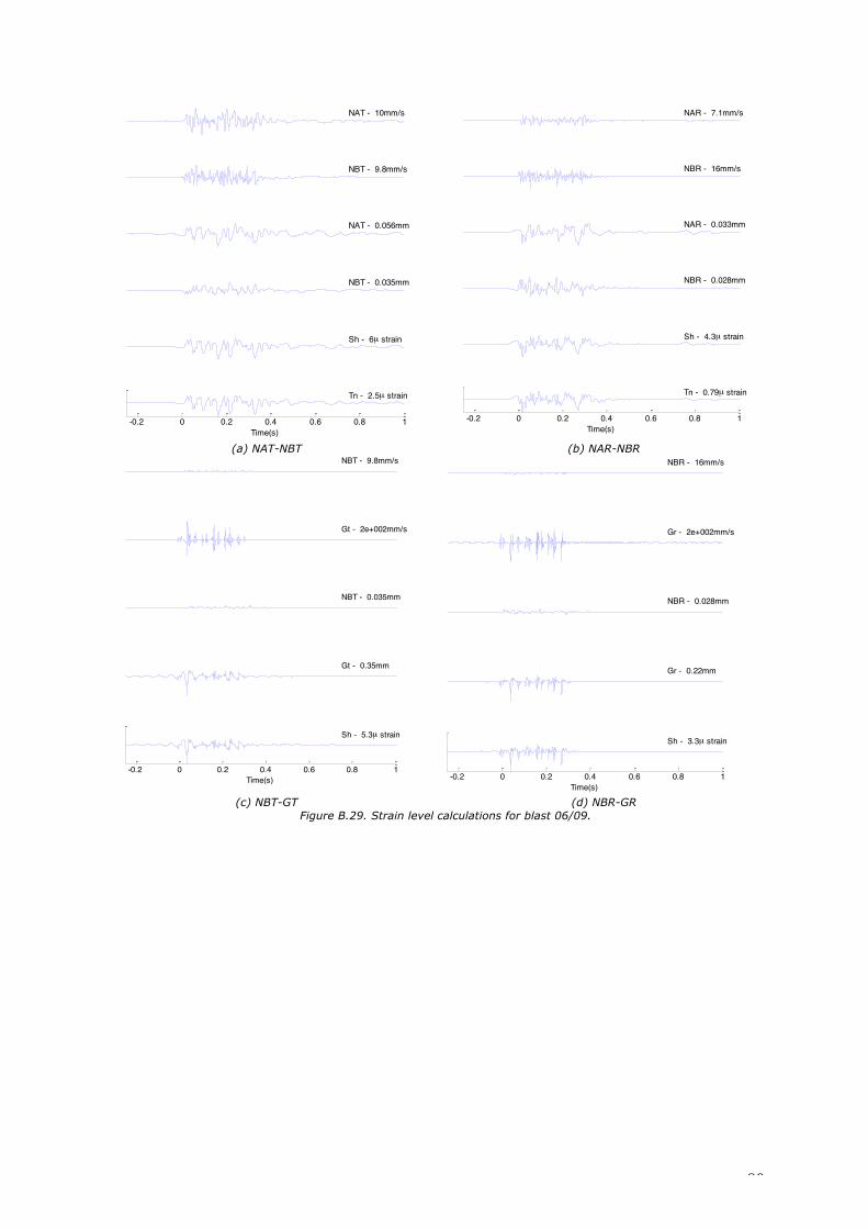
80
(a) NAT-NBT (b) NAR-NBR
(c) NBT-GT (d) NBR-GR
Figure B.29. Strain level calculations for blast 06/09.
NAT - 10mm/s
NBT - 9.8mm/s
NAT - 0.056mm
NBT - 0.035mm
Sh - 6µ strain
-0.2 0 0.2 0.4 0.6 0.8 1Time(s)
Tn - 2.5µ strain
NAR - 7.1mm/s
NBR - 16mm/s
NAR - 0.033mm
NBR - 0.028mm
Sh - 4.3µ strain
-0.2 0 0.2 0.4 0.6 0.8 1Time(s)
Tn - 0.79µ strain
NBT - 9.8mm/s
Gt - 2e+002mm/s
NBT - 0.035mm
Gt - 0.35mm
-0.2 0 0.2 0.4 0.6 0.8 1Time(s)
Sh - 5.3µ strain
NBR - 16mm/s
Gr - 2e+002mm/s
NBR - 0.028mm
Gr - 0.22mm
-0.2 0 0.2 0.4 0.6 0.8 1Time(s)
Sh - 3.3µ strain


