
EXPORTS AND ECONOMIC GROWTH RELATIONSHIP IN KENYA:
CAUSALITY AND COINTEGRATION ANALYSIS (1970 - 2004) fj
B Y
KARIUKI GODFREY MACHARIA C/50/7743/2004
UN IVERS ITY OF NA IROB, ^ S T A F R ( O A N A . O U E C R T ? OJ
RESFARCH PAPER SUBMITTED TO THE SCHOOL OF ECONOMICS, UNIVERSITY OF NAIROBI, IN PARTIAL FULFILMENT FOR THE AWARD OF
THE DEGREE OF MASTER OF ARTS IN ECONOMICS
University ol NAIROBI Library
0369983 2
mv n K£NY .'->Tr A ML MORML
JULY 2006

DECLARATION
This Research Paper is my original work and has not been presented for a degree course in any
other University.
rS-Sr: Date:
GODFREY MACHARIA KARIUK1
n / o
This Research Paper has been submitted for examination with our approval as University
supervisors
Date
DR. HELLEN OMMEH
n N U * * (=>
^ S t ^ T A Date:
MR. DANIEL ABALA
[diJAQ.
Research Paper by Kariuki G. M. C/50/7743/2004for M.A. (Earn), UO!\' Page ii

TABLE OF CONTENTS Declaration - 1 1
Acknowledgement ' v
Dedication Vl
List of Abbreviations vii List of Tables and Figures viii Abstract i x
CHAPTER ONE: INTRODUCTION AND BACKGROUND 1 1.1. Introduction 1 1.2. Kenya's Economic Growth Performance 2 1.3. Kenya's International Trade Performance 4
1.3.1 Structure and Composition of Exports 7 1.3.2 Structure and Composition of Imports 9 1.3.3 Kenya's Trade Policy 9
1.4. Conceptual Framework 11 1.5. Problem Statement 12 1.6. Research Objectives 13 1.7. Justification and Significance of the Study 14
CHAPTER TWO: LITERATURE REVIEW 16 2.1. Theoretical Literature '. 16 2.2. Empirical Literature 20
2.2.1 Cross-sectional Studies 21 2.2.2 Country-specific Studies 22 2.2.3 Case Studies of Kenya 24
2.3. Overview of the Literature Review 26
CHAPTER THREE: METHODOLOGY 29 3.1. Theoretical Framework 29 3.2. Analytical Framework - The Model 30 3.3. Hypotheses to Be Tested 32 3.4. The Variables 32 3.5. Econometric Approach 34 3.6. Data Type and Sources 35 3.7. Unit Root Tests 35 3.8. Causality Analysis 36 3.9. Cointegration Analysis 38
* 3.10. Error Correction Mechanism 40
CHAPTER FOUR: EMPIRICAL RESULTS AND DISCUSSIONS 42 4.1. Summary Statistics and Graphical Analysis 42 4.2. Stationarity Properties 43 4.3. Causality Results and Interpretation 44 4.4. Cointegration Results and Discussions 46
CHAPTER FIVE: CONCLUSIONS AND POLICY IMPLICATIONS 51 5.1. Policy Implications 52 5.2. Study Limitations and Research Agenda 54
REFERENCES 56 Appendix I: Graphica l Analysis 59
Research Paper by Kariuki G. M. C/50/7743/2004for M.A. (Earn), UO!\' Page ii

ACKNOWLEDGEMENT
I am gratified to express deep, heartfelt and special gratitude to my university supervisors, namely.
Dr. Hellen Ommeh and Mr. Daniel Abala for their professional guidance, sacrifice, encouragement,
patience and cordial working relationship, which greatly contributed to successful completion of
this research project. Precisely, their assistance was very beneficial. My fruitful discussions with the
supervisors coupled with their constructive comments, positive suggestions, tireless efforts and
unwavering support were indeed wonderful inspiration and fulfilling experience to me.
My sincere thanks equally go to my MA (Econ) lecturers, including Prof. G.M. Mwabu. Prof. F.M.
Mwega. Dr. D.M. Kulundu. Dr. R.W. Ngugi and others for rigorously imparting economics
discipline deep in my mind and their meticulous and valuable professional advice on research
methodology, an experience that I will never forget. Indeed, my interactions and discussions with
the lecturers gave me a lot of hope and determination in pursuing economics as a profession. I
would also like to sincerely thank my 2004/2006 classmates, including Joseph Muraga. Winnie
Karingithi, Joseph Gichimu, Joel Imitira, Yusuf Mbuno, Boniface Kariuki, Daniel Kamande,
Patricia Mukere. Fredrick Wamalwa and others, who unknowingly partly contributed to the success
of this paper, for their effective discussions and moral support. Special thanks go to Timothy
Kariuki for also being a helpful discussant of my research proposal. In fact, I was also encouraged
by my colleagues' enjoyable cooperation during the entire course, particularly the confidence they
bestowed on me to chair several group discussions.
I take this opportunity to pass my warm gratitude to the Government of Kenya, particularly the
Ministry of Cooperative Development and Marketing, for funding my MA (Econ) course. I am
especially grateful to the Permanent Secretary. MOCDM. who recognized the relevance of the
course and approved the sponsorship. I am also very thankful to African Economic Research
Consortium (AERC) for sponsoring me in their 2005 Collaborative Masters Programme (CMAP)
Joint Facility for Electives (JFE) in Karen. Nairobi and supporting this research project.
Deep in my heart I am greatly indebted to my wife Tabitha and our sons Timothy and Martin for
their understanding, tolerance and moral support that went a long way to make me succeed in my
MA course. They never accused me of domestic negligence and this is truly wonderful. I admire the
way my wife stood by me. accepted the loneliness and her understanding why I was spending long
and odd hours with books and computer.
Research Paper by Kariuki G. M. C/50/7743/2004for M.A. (Earn), UO!\' Page ii

I watched helplessly as Timothy wondered why Dad's "homework" was endless while Martin could
not understand why Daddy was hiding with books. Precisely, they inspired me and encouraged me
to soldier on and I am extremely happy that the young boys developed a culture of reading,
especially Martin at a tender age of two years. They truly deserve dedication and my sincere
apologies go to them for any missed attention.
Lastly and most important, I thank the Almighty God for His unfailing love, mercy and spiritual
support to me, giving me an opportunity to take the MA course and the successes that I have
achieved during my entire academic life. Actually, it is God ' s blessings, without which I could not
have done anything, that enabled me to study with a lot of hope, confidence, determination and
courage. I witnessed the miraculous hand of the Lord that saved and supported me at times when
failure and desperation were almost imminent during my studies.
All in all, any mistakes in this paper solely remain mine.
Research Paper by Kariuki G. M. C/50/7743/2004for M.A. (Earn), UO!\' Page ii

DEDICATION
I dedicate the entire MA (Econ) course to Tabitha, Timothy and Martin and this research project to
my parents. Joseph Kariuki and Catherine Wambura, who sensitized me on the essence of hard
work and the benefits of academic excellence, with a lot of passion when I was young.
Research Paper by Kariuki G. \1. C/50/7743/2004for M.A. (Econ), L O.\ Page 6

List of Abbreviations
ACP African. Caribbean and Pacific ADF Augmented Dickey-Fuller AIC Akaike Information Criterion AU African Union AGOA African Growth and Opportunity Act ASEAN Association of South East Asian Nations CBS Central Bureau of Statistics COMESA Common Market for Eastern and Southern Africa CRDW Cointegrating Regression Durbin Watson EAC East African Cooperation ECM Error Correction Model ECT Error Correction Term EG Engle-Granger ELG Export-led Growth ELGH Export-led Growth Hypothesis EPA Economic Partnership Agreement EPC Export Promotion Council EPPO Export Promotion Programmes Office EPS Export Promotion Strategy EPZ Export Processing Zones EU European Union FDI Foreign Direct Investment GDP Gross Domestic Product GLE Growth-led Exports GNP Gross National Product IFS International Financial Statistics IGAD Inter-Governmental Authority on Development IMF International Monetary Fund IRF Impulse Response Function ISS Import-Substitution Strategy KETA Kenya Export Trade Authority LDCs Least Developed Countries LM Lagrangian Multiplier MUB Manufacturing Under Bond NEPAD New Partnership for African Development NICs Newly Industrialized Countries OLS Ordinary Least Squares PP Phillips and Perron PTA Preferential Trade Area RESET Regression Specification Error SBC Schwartz Bayesian Criterion SEA South East Asia SSA Sub-Saharan African SUR Seemingly Unrelated Regressions UNCTAD United Nations Conference on Trade and Development USA United States of America VAR Vector Autoregression VECM Vector Error Correction Model WTO World Trade Organization
Research Paper by Kariuki G. \1. C/50/7743/2004for M.A. (Econ), L O.\ Page 7

List of Tables and Figures
Page No.
Figure 1: Kenya's Volume and Balance of Trade - Kshs Billions (1994 - 2004) 6
Table 1.1: Kenya's Trade and GDP Analysis 7
Table 1.2: Domestic Exports of Principal Commodities as % of Total Export 8
Table 4.1: Summary Statistics 42
Table 4.2: ADF Unit Roots Tests 43
Table 4.3: Granger Causality Tests 44
Table 4.4: Long-run Relationship 47
Table 4.5: Short-run Relationship 48
Research Paper by Kariuki G. \1. C/50/7743/2004for M.A. (Econ), L O.\ Page 8

A B S T R A C T
The relationship between exports and economic growth has been analysed for a long period.
Whether exports expansion cause economic gains or losses, whether economic growth causes
exports expansion or reduction, and whether a feedback relationship exists between exports growth
and economic growth has been a recurring empirical problem. Empirical evidence linking exports to
economic growth has been mixed and inconclusive due to fundamental differences in methodology,
analytical techniques, sample period and study countries.
This study examines the exports-growth relationship in Kenya using secondary annual time series
data for 1970 - 2004. Particularly, the study investigates export-led growth hypothesis for Kenya by
testing for Granger causality between exports growth and economic growth. The study also
investigates the long-run nature of the export-growth relationship by applying cointegration analysis
and error correction mechanism to estimate an augmented simple production function using
ordinary least squares method. Inclusion of exports and imports provides an alternative procedure to
capture total factor productivity growth. By considering relevant variables omitted in previous
studies for Kenya and by covering both imports-substitution and export-promotion eras, including
trade liberalization period, help clarify and improve past empirical results and minimizes the
existing knowledge gap.
The results of this study indicate that there is unidirectional causality from exports growth to
economic growth and by disaggregating exports into primary and manufactured exports; the
unidirectional causality is from primary exports to economic growth. There is a significant long-run
relationship between economic growth, exports, imports and capital formation. The study further
reveals significant long-run positive impact of exports, particularly primary exports on economic
growth while manufactured exports" impact, though positive is insignificant. On the other hand, the
short-run effects of both primary and manufactured exports are negative. Considering that Kenya
has been experiencing low, slow and unstable economic growth, coupled with rising poverty and
unemployment levels, this study concludes that primary exports-led growth is undesirable for
economic development. Therefore, primary exports should not be relied upon further as "engine of
growth", since this is unfavourable to Kenya's economic prosperity. Instead, more resources should
be directed towards value-addition of primary exports and growth and competitiveness of
manufactured exports.
Research Paper by Kariuki G. \1. C/50/7743/2004for M.A. (Econ), L O.\ Page 9

CHAPTER ONE: INTRODUCTION AND BACKGROUND
1.1. Introduction
Economic growth and development is a fundamental goal of any economy. While economic
growth is viewed as a process involving the entire economy's output performance, it
invariably depends on the productivity of a country. The sources of productivity growth and
productivity differences among countries and regions have today emerged as a central
unifying theme of growth and development. Particularly, the study of the role of exports on
economic growth is a recurrent research theme in trade and development literature and the
role of exports has been widely acknowledged. Although most research work have
emphasized on trade-growth relationship, it has been stressed that exports is only one of the
variables in output growth equation. Indeed, the idea that exports growth is a major
determinant of output growth, the export-led growth hypothesis (ELGH), has considerable
appeal to many developing countries due to positive externalities and other exports benefits.
Lately the export-led growth (ELG) paradigm has received a lot of attention following the
highly successful East Asian export-led growth strategy during the 1970s and 1980s, and
especially if compared to dramatic failures of import-substitution policies in most Latin
America and African countries. Earlier empirical studies generally concluded that there is
strong evidence in favour of ELGH. However, recent time series studies have generally
concluded that the statistical evidence in favour of exports-promotion per se is not as
unanimous as was previously thought. It is also possible that export promotion policies may
only increase exports in the long-run. Consequently, internally generated growth-led exports
hypothesis (GLEH) has been tested with supportive evidence. In fact renewed emphasis is
now placed on the role of internal factors or basic characteristics of an economy, such as
infrastructure, human capital, institutions and entrepreneurship. which reduce production
costs of tradables thus improving their international competitiveness.
After independence Kenya experienced impressive economic performance. However, the
1970s was a period of external shocks, which adversely affected balance of payments and
economic growth mainly due to the rigid, inward-looking and price-distorting imports-
substitution strategy that was being implemented.
Research Paper by Kariuki G. \1. C/50/7743/2004for M.A. (Econ), L O.\ Page 1

This prompted the introduction of exports-promotion strategies and structural reforms in early
1980s that culminated into a liberalized economy by early 1990s.
The available supportive evidence in favour of ELGH and global trend towards trade
liberalization appears to have influenced Kenya to adopt the ELG strategy. However, unlike
the fast growing Asian countries, which were at the same development level with Kenya in
1960s. Kenya has not been successful in gaining a competitive export sector and has been
experiencing slow and low economic growth with increasing poverty and unemployment
levels. So what went wrong for Kenya and when and how did this happen? What lessons can
Kenya learn from the Asian experience? During 1960s and early 1970s, when Kenya
promoted ISS and exports performed poorly, the country had impressive economic growth
record. After the structural reforms, when export performance improved, economic growth
has been slow and inadequate. This has led to the question whether export promotion can be
relied upon for economic growth in Kenya or is it economic growth that should precede
exports promotion. Consequently, there is need to understand the nature of exports-growth
relationship in Kenya. This forms the basis of the research problem addressed by this study.
The study therefore examines the causality direction and nature of the exports-growth
relationship in a simple growth model.
This paper is organized into five chapters. Chapter One on introduction and background
briefly discusses Kenya's economic growth and trade performances and also talks about the
research problem, study objectives and justification. Chapter Two provides both theoretical
and literature review and Chapter Three outlines the methodology used. Chapter Four
discusses and interprets the empirical results while Chapter Five summarises the study
findings, highlights policy implications and proposes areas of further research.
1.2. Kenya's Economic Growth Performance
The pre-colonial Kenya economy was almost a wholly subsistence one, with very little trade
with Arab and European traders. The advent of colonial administration and immigrant
communities brought in development of markets, institutions and general monetization of the
economy. Kenya experienced improved economic performance during the first decade of
independence.
Research Paper by Kariuki G. \1. C/50/7743/2004for M.A. (Econ), L O.\ Page 2

The economy recorded faster and higher economic growth in the country's economic history
with an average growth rate of about 6%. This was followed by a period of poor performance
between mid 1970s and early 1980s mainly due to the effects of 1973 and 1979 oil shocks,
mismanagement of 1976/77 coffee boom, collapse of the East African Community in 1977,
1982 military coup attempt and a severe drought in 1983/84. This led to balance of payments
problems, with the average growth rate declining to 5.2% in 1974-79 and 3.2% in the first half
of 1980s (Mwega and Ndung'u, 2004).
Structural reforms were implemented from mid 1980s and the period 1985-1989 witnessed a
bit of economic recovery, with annual growth averaging 5%. The reforms, implemented up to
early 1990s, covered nearly all sectors of the economy, including liberalization of trade,
payments system, the foreign exchange market, domestic financial and capital markets,
privatization and commercialization of public enterprises. The first half of 1990s witnessed
worsening economic environment, with an average growth rate of 2.5%. There was a drought
in 1991/92. the oil price increase due to the Gulf war. compounded by the aid embargo of
1991-93 and "ethnic clashes" in 1992 (Mwega and Ndung'u. 2004). These exogenous shocks
were accompanied by an increase in budget deficit and excessive money supply, due to
unwarranted government spending on the 1992 elections. As a result, this rapidly increased
inflation rate from 27.3% in 1992 to about 46% in 1993 alongside large exchange rate
depreciations over the same period.
In the late 1990s, economic growth declined further to an average of 1.9%, coupled with aid
embargo of 1997-2000, "ethnic clashes" in the run-up to and after the 1997 elections. This
situation was exacerbated by unfavourable weather conditions, including the El Nino rains in
1997/98 followed by a major drought that occasioned power rationing, that culminated into
very poor economic growth of -0.2% in 2000 (Mwega and Ndung'u. 2004). Due to improved
weather and macroeconomic policies together with increasing economic integration. Kenya's
economy started recovering and witnessed an average growth rate of 1.2% in 2001-02. Some
sectors such as tourism, horticulture, transport and telecommunication registered remarkable
growth rates and this steered the economic growth to 1.8% in 2003, 4.3% in 2004 and 5.8% in
2005. The GDP growth rate is projected to rise over 6% in 2006 and beyond but the 2005/06
drought is expected to have a negative impact.
Research Paper by Kariuki G. \1. C/50/7743/2004for M.A. (Econ), L O.\ Page 3

1.3. Kenya's International Trade Performance
At independence, Kenya adopted an industrialization policy based on import-substitution
strategy (ISS) which was characterised by protective and prohibitive trade barriers, such as
high rates of protection, price controls, foreign exchange controls and import licensing. This
involved development of domestic industries via protection at the expense of exports growth.
Large proportion of the industrial output was meant for the domestic market, which was more
profitable than the export market. This discouraged export promotion and partly accounted for
the poor export performance of Kenya's manufacturing sector (Were et al., 2002).
By 1980s. Kenya had achieved a reasonable level of industrialization in the region but like in
most African and Latin American countries, the ISS failed to achieve the intended objectives
despite the considerable protection the industries enjoyed. With a series of external shocks in
1970s, e.g. the oil crises of 1973 and 1979 and the collapse of the East African Community in
1977. the inefficiency and inadequacy of the ISS became evident. The balance of payments
deteriorated such that by the end of the period the Government recognized the need for an
export-oriented strategy as articulated in the Development Plan of 1979-83, which aimed at
efficient industries, increased competitiveness and diversification of exports (Kundhi (1996).
In the early 1980s, partly due to the increasing pressure, mainly from World Bank and IMF,
for structural adjustment reforms. Kenya government embraced liberalization policy, a major
component of which was a shift from ISS to export-promotion strategy (EPS). In mid-1980s,
a key policy milestone was the publication of the Sessional Paper No. 1 of 1986 on Economic
Management for Renewed Growth, in which liberalization and outward-looking development
strategies were adopted. By this time. Kenyan exports had deteriorated tremendously.
Merchandise export earnings as a percentage of GDP had for example declined from 19.6% in
the 1970s to 16.97% over 1980-84 and 13.6% over 1985-89 (Were et al., 2002).
In addition to the export compensation scheme established in 1976, a number of export
promotion programmes were initiated. These include the Green Channel in 1988, Export
Guarantee and Credit Scheme, Preferential Trade Area (PTA). revival of the Kenya Export
Trade Authority (KETA) in 1976, establishment of Export Promotion Council (EPC) and the
Export Promotion Programmes Office (EPPO) for tax rebates on imported inputs for exports.
Research Paper by Kariuki G. \1. C/50/7743/2004for M.A. (Econ), L O.\ Page 4

This also included establishment of Manufacturing Under Bond (MUB) in 1988 and Export
Processing Zones (EPZ) in 1989/90. It was observed that although in the long-run the best
incentive for exports expansion is flexible management of the exchange rate, the above
incentives were necessary1 to encourage potential exporters to make investments and break
into the foreign markets (GoK, 1986).
However, export incentives notwithstanding, export orientation in the 1980s remained weak
largely due to very high effective rates of protection accorded to domestic industries,
exchange rate bias against exports, high cost of imported inputs, foreign exchange controls,
administrative delays and high transaction costs among others (Were et al., 2002). The export
incentives also remained unattractive and less successful due to weaknesses in
implementation and poor coordination. There were initial attempts to liberalize imports during
1980-84 and 1988-91. but these were also less successful. These shortcomings called for
further reforms so as to get any meaningful trade benefits. This ushered in trade liberalization
era in the early 1990s.
Trade liberalization properly started in the 1990s with a conversion of quantitative restrictions
to tariffs equivalents and the Government embarked on phased tariff reductions and
rationalization of the tariff bands. The most significant shift in trade policy regime came in
May 1993 with the abolition of trade licensing requirements and more importantly,
liberalization of the foreign exchange market. During the period 1993-94. all current and
capital accounts restrictions were lifted and there was immense response on both imports and
exports. Nevertheless, the response on the exports was combined with a price effect
occasioned by the steep depreciation of the Kenya shilling from Kshs 36.22 in 1992 to Kshs
68.16 per US dollar in 1993. Exports earnings rose dramatically from 13% of GDP in 1992 to
over 20% between 1993 and 1996 (Were et al., 2002). This recovery was also brought about
by macroeconomic reforms and increasing regional integration under the East African
Cooperation (EAC) and the wider Common Market for Eastern and Southern Africa
(COMESA).
Research Paper by Kariuki G. \1. C/50/7743/2004for M.A. (Econ), L O.\ Page 5

Figure 1: Kenya's Volume and Balance of Trade - Kshs Billions (1994 - 2004)
MO
500
400
300
] 1 200
I
100
0
-100
-200 Year
—«— Export* —•—lapim —•—Trmd* Bahan - » Trade Volume
Source: C B S Statistical Abstracts
Figure 1 shows the general trends of Kenya's trade volume including exports, imports and
trade balance for the period 1994-2004. Over the last decade, Kenya's trade volume has
increased more than twofold from Ksh 201 billion in 1994 to Ksh 579 billion in 2004. Total
exports have increased from Ksh 86 billion to Ksh 215 billion, an increase of 150%, while
imports have increased from Ksh 115 billion to Ksh 364 billion, which is an increase of about
217%, over the same period. It is clear therefore, imports have increased more than exports
and this put Kenya on a trade deficit that increased from Ksh 29 billion in 1994 to Ksh 149
billion in 2004 although the deficit had declined to Ksh 99 billion and 88 billion in 2003 and
2002 respectively.
Table 1.1 below shows shares of Kenya's exports, imports and trade volume in GDP, shares
of primary and manufactured exports in domestic exports, exports/imports ratio and real GDP
and exports growth rates for three periods. The periods 1970-80, 1981-93 and 1994-2004
represents imports-substitution, export promotion and trade liberalization periods
respectively. For the past decade, the exports/GDP ratio has on average been 19.4%,
imports/GDP ratio has been around 32.2%, trade openness on average has been 51.5% and
imports cover has been 60.6%.
Research Paper by Kariuki G. \1. C/50/7743/2004for M.A. (Econ), L O.\ Page 6

Real GDP growth has continued to decline from an average of 5.0% in 1970-80 to 3.3% in
1981-93 and 2.4% in 1994-2004. Real exports growth rate remained constant at about 2.65%
in 1970-93 but increased to 3.7%, indicating the positive impact of trade liberalization.
Table 1.1: Kenya's Trade and GDP Analysis
Expo rts / GDP
Imports/ GDP
Primary Exports/ Exports
Manuf. Exports/ Exports
Trade Vol./ GDP
Exports/ Imports
Real GDP r.
Real exports
S- r. 1970 -1980
0.268 0.583 0.863 0.161 0.851 0.466 0.050 0.027
1981 -1993
0.172 0.262 0.842 0.191 0.434 0.666 0.033 0.026
1994-2004
0.194 0.322 0.745 0.345 0.515 0.606 0.024 0.037
Source: Author's computation from CBS Statistical Abstracts: g. r. - growth rate
1.3.1 Structure and Composition of Exports
Like most developing countries, Kenya's export trade is predominantly composed of primary
commodities mainly tea, horticulture and coffee besides tourism. The three primary products
together with petroleum products and cement account for over two thirds of total foreign
earnings (GoK, 2004). As it is evident in Table 1.1 above, primary exports represents about
75% of domestic exports. The Kenyan exports are therefore more vulnerable to world prices
fluctuations. Although horticultural exports have grown in the last few decades, manufactured
exports make a small proportion of total exports. However, the share of manufactured exports
in total exports has increased since 1994, mainly due to trade liberalization. All in all, export
growth has been highly erratic, based on fluctuating earnings of the primary exports and the
tourism sector.
Until the late 1980s, coffee exports contributed the largest share of about 32% to total
commodity exports, with notable performance in 1977 and 1986. which was attributed to
positive price shocks in the world market, especially the severe frost in Brazil in 1977 that
resulted into the "coffee boom" for Kenya (Were et al., 2002). Of late the performance of the
coffee sector has continued to worsen and has been overtaken by horticultural and tea exports.
Research Paper by Kariuki G. M. C/50/7743/2004for M.A. (Earn), UO!\' Page ii

Table 1.2: Domestic Exports of Principal Commodities as a percent of Total Value of
Commodities Export
Tea Coffee
(not roasted) Horticulture Petroleum products
Cement (building)
1994 20.2 15.6 10 6.1 2 1995 19.3 15.5 11.4 4.7 1.7 1996 19.9 14.4 12 6.2 2.2 1997 21.1 14.7 12 9 2 1998 28.8 11.2 8.2 8.5 1.3 1999 28.6 10.4 15.4 7.9 1.1 2000 29.3 9.8 17.7 7.9 1.1 2001 28.4 6.1 16.3 10.2 0.8 2002 26.2 5 21.6 3 1.1 2003 24.1 4.6 26.7 0.1 1.4 2004 22.7 4.4 24.9 0.7 1.2
Source: Central Bureau of Statistics, Statistical Abstracts
However, as indicated in Table 1.2 above, since the early 1990s tea exports took the lead up
to 2002. However, starting from 2003. horticultural exports took the lead of 26.7% of total
domestic commodity exports, followed by tea exports. In 2003. tea and horticulture exports
together accounted for 50.8% of the total domestic exports earnings (GoK, 2004). As
reflected in Table 1.2, in 2004 the combined share of horticulture, tea and coffee accounted
for 52% of total value of commodity exports, reflecting the dominance of agricultural
commodity exports.
From mid 1990s, Kenya's domestic exports have been rising with the largest share generally
going to Africa. Out of the total domestic exports value of about Ksh 159 billion in 2004,
approximately 39 % or Ksh 62 billion went to African countries. Regional integration
measures under the EAC and the wider COMESA and economic recovery and trade
liberalization initiatives in the region are some of the factors accounting for this dominance
exports share. The main countries of destination in Africa include Uganda, Tanzania, Egypt,
Sudan. DR Congo, Rwanda and Somali. Tanzania was a member of COMESA up to Sept
2000.
Research Paper by Kariukl G. XI. C/50/7743/2004for V/..4. (Econ), VON Page 8

Beyond Africa. Europe has maintained the biggest share of Kenya's domestic exports. In
particular, the European Union (EU) is the second destination of Kenya's exports after
COMESA. For example in 2004, out of the total value of exports to Europe of about Ksh 59
billion. 95% or Ksh 56 billion went to the EU. which represented 35% of total exports. The
main countries of destination in the EU include United Kingdom (UK), Netherlands,
Germany, France and Belgium. Over the world, other key countries of destination include
United States of America (USA), Pakistan, India and Yemen.
1.3.2 Structure and Composition of Imports
Over the years, Kenya's imports have been increasing. The imports mainly consist of
intermediate inputs and machinery. These includes crude petroleum, gas and diesel oils,
vegetable fats and oils, kerosene, jet fuel, synthetic plastic materials, medical and
pharmaceutical products, telecommunication equipment, motor vehicles and their parts. For a
long period Kenya's imports have mainly originated from Europe followed by Middle East
and Far East. However, Kenya's search for new markets and trade relations have borne fruits
since in 2004 the largest share of imports came from the Middle East followed by Europe and
Far East. In Europe, as was the case of exports, EU is the main source of imports.
In Africa unlike the case of exports, Kenya's imports are mainly from South Africa, a non-
COMESA member country. For instance in 2004. out of the total imports from Africa valued
at Ksh 52 billion, imports from South Africa amounted to Ksh 35 billion or 67% while from
COMESA countries imports amounted to 29% or about Ksh 15 billion. In Asia, the main
countries of origin of Kenya's imports include Saudi Arabia. Bahrain, Japan, India and
mainland China.
1.3.3 Kenya's Trade Policy
The import substitution strategy adopted in Kenya at independence created an anti-export bias
that led to unfavourable export growth performance especially of manufactured exports.
However, starting in the mid-1980s, Kenya shifted away from an ISS trade regime towards a
more outward-oriented growth policy. With globalization, export-led growth strategy has
become a major focus for many countries including Kenya, particularly in consideration of
development constraints facing the country such as limited external financing.
Research Paper by Kariukl G. XI. C/50/7743/2004for V/..4. (Econ), VON Page 9

As articulated in GoK (2003), it has been recognized that trade and export promotion are
crucial components of a sustainable economic growth strategy. The principle objectives are to
reduce the cost of doing business, eliminate impediments to supply chains, and introduce
appropriate policy, regulatory and institutional reforms conducive for sustained economic
growth in Kenya.
To promote exports growth a number of schemes to reduce and/or eliminate import taxes on
inputs for exportable goods, as well as providing other incentives to exporters have been
implemented. These include a duty suspension program, bonded warehousing and
manufacturing facilities, and export processing zones. Kenya's general trade policy objectives
include moving towards a more open trade regime, strengthening and increasing overseas
market access for Kenyan products, and further integrating the country into the world
economy. These policy objectives have been pursued through unilateral trade reforms,
multilateral, regional and bilateral trade agreements.
Besides being a member of the World Trade Organization (WTO), Kenya is a participant in
various regional, sub-regional and international trade initiatives, including the EAC,
COMESA. 1GAD. the A U ' s NEPAD. ACP - EU agreement and USA's AGOA. With the
launching of EAC's customs union, a similar arrangement to follow under COMESA. the
evolving trade arrangement with the EU under the EPA and the scheduled completion of
WTO's Doha Development Agenda, Kenya's integration with the rest of the world is about to
change significantly during the coming years. In particular, there are potential export
opportunities that include product and market diversification.
In light of the potential benefits of export promotion in economic growth, increased outward
orientation of the Kenyan trade policy is expected to have beneficial growth effects in the
economy. However, it is worth noting that even though Kenya has adopted a flexible
exchange rate system, which is an appropriate policy, the response of manufactured exports to
price incentives has not been very good. This could have been due to structural and
institutional constraints such as inadequate and poor infrastructural facilities (Kasyoka, 1999).
Hence in the long-run. the appropriate price policy must be supported by structural and
institutional policy measures.
Research Paper by Kariukl G. XI. C/50/7743/2004for V / . . 4 . (Econ), VON Page 10

However, it must be observed that a major stumbling block to trade reforms that encounter
developing countries like Kenya is the potential loss of customs revenues due to reduction in
tariffs. In Kenya import duties have represented a declining, but still important, component of
government revenues. Import duty as a proportion of total current revenue averaged 20%
before 1984. This declined to about 15% between 1985 and 1999 and from 2000 this has gone
down to an average of 10%. However, although import duties share of government revenues
has declined, there is evidence that revenue collection has increased relative to the reduction
of tariffs, due to improved tax administration.
1.4. Conceptual Framework
The relationship between exports and economic growth has been analysed for a long period.
The export-led growth hypothesis postulates that export growth is one of the key determinants
of economic growth and hence exports growth acts as a catalyst for income growth. Exports
are known to have both direct and indirect effects that positively affect economic growth. The
main exports benefits, or the channels through which total factor productivity is increased,
includes foreign exchange earnings, resource allocation according to comparative advantage,
exploitation of economies of scale, improved production techniques, greater capacity
utilization, positive externalities on non-exports, more efficient management styles and
increased employment. Growth performance in most developing countries is constrained by
shortage of foreign exchange and therefore these countries could grow faster with more
exports.
The ELGH assumes causality direction from exports to economic growth but in some cases
due to lack of competitiveness, manufactured exports particularly for developing countries,
negatively affects economic growth. The opposite causality direction implies growth-led
exports hypothesis (GLEH). This is grounded on the potential benefits of first developing the
domestic economic environment. This works out when the growth of domestic economy
boosts exports growth, but in some cases national income growth can result to increased
domestic consumption of exportables thus reducing exports. Empirical evidence linking
exports to economic growth has been mixed and inconclusive. The available supportive
evidence in favour of ELGH and global trend towards trade liberalization appears to have
influenced Kenya to adopt the ELG strategy.
Research Paper by Kariukl G. XI. C/50/7743/2004for V/..4. (Econ), VON Page 11

The ELG strategy is envisaged in several Kenya's policy documents, including Sessional
Paper No. 1 of 1986 on Economic Management for Renewed Growth. Sessional Paper No. 2
of 1997 on Industrial Transformation to the Year 2020 and the Economic Recovery Strategy
for Wealth and Employment Creation (2003-2007). Therefore, has Kenya really experienced
exports-led growth, growth-led exports or feedback between exports and economic growth?
Has there been any long-run relationship between exports and economic growth?
Consequently, there is need to understand causality direction and the nature of exports-growth
relationship in Kenya. This forms the basis of the research problem discussed in the next
section.
1.5. Problem Statement
Whether exports expansion cause GDP gains or losses, whether GDP growth causes exports
expansion or reduction, and whether a two-way causal relationship exist between exports
growth and GDP growth can only be decided empirically, preferably for individual countries.
However, in some cases these relations have been frequently invoked without detailed
empirical proof. Although the theoretical links between trade and economic growth has been
discussed for over two centuries, controversy still persists regarding their real effects.
However, over the last four decades substantial amount of research concerning the association
between exports and growth has been carried out in both developed and developing countries
fundamentally differing on methodology, analytical techniques, sample period, study
countries and hence their results.
Does rapid income growth lead to rapid trade expansion or is it the other way round?
Subjective evidence suggests that countries with strong exports performance have strong
growth performance and vice versa. Bhagwati (1988) as cited by Henriques and Sadorsky
(1996) suggests that, as with most economic phenomena, there is a reciprocal relationship
between the two economic indicators. Indeed many developing countries have been pursuing
aggressive export promotion strategies and some countries have actually achieved rapid
economic growth. While earlier empirical work indicates that there is positive correlation
between exports growth and economic growth, questions about causality direction remains
unanswered.
Research Paper by Kariuki G. \1. C/50/7743/2004for M.A. (Econ), L O.\ Page 12

Therefore, the main research problem is to find out whether specific countries or group of
countries have been experiencing export-led growth or growth-driven exports. Both positive
and negative signs are expected in either causality direction i.e. in case of ELG, there can be
growth-reducing exports and in case of GLE, there can be exports-reducing growth. This
research thus solidly concurs with Jung and Marshall (1985) that tests of ELGH should focus
on the causality direction as well as the sign of the relationship. Hence there is a problem of
deciding causality direction and determining the sign, magnitude, significance and nature of
the relationship between exports and economic growth. This is the research problem
addressed in this study using the case of Kenya.
Kenya adopted imports-substitution strategy in 1960s and 1970s and export-promotion
strategy from early 1980s. Economic growth was remarkable in 1960s but from mid-1970s, it
was adversely affected by external shocks with resultant poor performance mainly due to
rigidity of the ISS. This led to the adoption of exports-promotion strategy and structural
reforms that culminated into liberalization in early 1990s. Since then, economic growth has
been slow, low and wanting. This study investigates the causal relationship between exports
growth and economic growth in Kenya for the period 1970 - 2004. It is an attempt to answer
the questions: is export-led growth hypothesis or growth-led exports hypothesis valid for
Kenya? Eleven years after trade liberalization, what is still going wrong that is adversely
affecting Kenya's growth path? Could the poor growth performance be attributed to the nature
of exports-growth relationship? The study therefore tests the ELGH for Kenya and attempts to
address the extent to which exports growth drives GDP growth in a long-run relationship.
This study therefore is an addition to the prevailing literature on the exports-growth
relationship and it contributes towards minimising the existing knowledge gap.
1.6. Research Objectives
The overall objective of this study is to examine exports-growth relationship in Kenya.
Specifically, this research aims at achieving the following objectives:-
(i) To examine causality direction between exports growth and economic growth
in Kenya;
Research Paper by Kariuki G. \1. C/50/7743/2004for M.A. (Econ), L O.\ Page 13

(ii) To investigate and estimate long-run relationship between exports and
economic growth in Kenya; and,
(iii) To draw policy implications from the results of (i) and (ii) above.
1.7. Justification and Significance of the Study
This study is interested in investigating causality direction and estimating long-term
relationship between exports and economic growth in Kenya during the period 1970 - 2004.
This period is significant in Kenya's economic history since it covers the imports-substitution
era of 1960s and 1970s, the shift to export-promotion strategy in early 1980s and
liberalization era from early 1990s. Kenya is a developing country, whose economy
participates in international trade, has been affected by external shocks and the country is a
major economic player in the region. Hence, improvement of Kenya's economy is a boost in
the region and the other regional countries can learn from Kenya's economic growth
experience. The author is also well conversant with Kenya.
This study recognizes the weaknesses of cross-sectional studies and acknowledges the
limitations, omissions and recommendations of time series studies. The study hence adopts
time series analysis approach using a case study of Kenya. Non-existence of feedback
between exports and economic growth justifies use of OLS as opposed to system methods.
Although there has been past attempts to study exports-growth relationship in Kenya,
individual case studies are few. Most of the previous studies are not comprehensive while
others are not specific to Kenya. Those studies that have analyzed Kenya individually using
time series analysis did so in a different economic environment and applying different
methodologies. Kundhi (1996) recommended that a similar time series study should be carried
out in the long-run when Kenya's trade regime is more outward-looking and long after trade
liberalization.
This research therefore, recognizes the gaps left by past empirical studies and attempts to fill
the existing information gap. Eleven years after trade liberalization in Kenya, this study
attempts to analyse the exports- economic growth relationship, thus it is more up-to-date.
Research Paper by Kariuki G. \1. C/50/7743/2004for M.A. (Econ), L O.\ Page 14

The study employs a multivariate time series analytical framework using neoclassical growth
model. Granger causality tests, cointegration and error correction analysis. This study is also
different from past empirical work because it analyses additional causality relationships that
are closely related with exports-growth link such as exports-imports and imports-growth
relationships, which strengthens the results of the study. The analysis is extended to consider
whether trade liberalization affected trade and economic growth in Kenya. This kind of
analysis has not been carried out by past studies.
This research not only examines the effectiveness of Kenya's export promotion strategies but
also evaluates the success of the various economic policies adopted since 1970s and their
reliability for sustainable economic growth and development. By finding out whether there
exists a long-run relationship between exports and economic growth in Kenya and
discovering the causality direction, this study serves as a policy guide by attempting to answer
the questions: Has Kenya been successful in the pursuit of export-led growth? Should Kenya
pursue exports promotion first or should it first develop the domestic economy?
The findings of this study are quite informative and point out several issues of policy concern.
Particularly, the results will help policy makers to evaluate various trade policies, including
their impact on trade performance, particularly the exports sector, and the overall economy.
The study will guide in policy prioritization and resource allocation in trade and growth
policies in Kenya. Time series analysis remains the most widely used approach for analysing
exports-growth relationship, hence it can be argued that the results of this study gives better
insight and measure of Kenya's long-run relationship between exports, imports and economic
growth.
Research Paper by Kariukl G. XI. C/50/7743/2004for V/..4. (Econ), VON Page 15

CHAPTER TWO: LITERATURE REVIEW
2.1. Theoretical Literature
The idea of trade originates from mercantilism doctrine of 16th century that underlined exports
as a means of increasing a country's wealth. Favourable arguments for free trade started with
the classical school of economic thought when Adam Smith's absolute advantage theory of
1776 highlighted the importance of trade as a vent for surplus production and the accruing
benefits of specialization. This was later improved by David Ricardo's comparative advantage
theory of 1817, which clearly documents the gains from international trade. Since then, the
role of exports in economic growth has been widely acknowledged and the link between trade
and economic growth has been extensively discussed worldwide. Theoretical literature mainly
focuses on the relationship between trade and economic growth in contrast to empirical
studies that have typically focused on the relationship between exports and economic growth.
Traditional classical economic theory argues that economic growth is a function of the factors
of production, mainly labour and capital. But in the last two decades there has been an
impressive activity on economic growth literature triggered by the endogenous growth theory,
which has led to an extensive inventory of models that stress the importance of trade, among
many other factors, in promoting sustainable economic growth. Recent models of economic
growth emphasises the role of increasing returns to scale and extend the neoclassical growth
model so that technological changes are endogenous and total factor productivity (TFP)
growth is responsive to policy. Total factor productivity is determined by several factors
including competition, uninterrupted growth, policy changes, institutions among others, all of
which tend to point to a trade-related environment (Onjala, 2002). Therefore, trade policy
affects productivity and growth with a general conclusion that countries that practice more
open trade tend to grow faster.
Out of the exports-growth debate, there are three possible relationships between exports and
economic growth, namely, export-led growth, growth-driven exports and feedback. Export-
led growth hypothesis postulates that export growth leads to economic growth and hence
exports act as an "engine of growth". On the other hand growth-led export suggests that rapid
economic growth leads to rapid export expansion.
Research Paper by Kariuki G. \1. C/50/7743/2004for M.A. (Econ), L O.\ Page 16

The advocates of ELGH have emphasized that trade has been the main engine of growth in
South-East Asia, whereby the Four Tigers: Hong Kong, Taiwan, Singapore and South Korea,
have achieved high economic growth because of their free-market outward-oriented strategies
(Medina-Smith, 2001). Within trade theory there are several reasons put forward by exports-
optimists to support exports-led growth strategy as opposed to imports-substitution strategy.
Afxentiou and Serletis (2000), Balassa (1978) and Kunst and Marin (1989) have pointed out
that exports benefits are derived from (a) exports concentrates investment in the most efficient
sectors of the economy - those in which the country enjoys a comparative advantage. This
improves allocation of resources from inefficient non-trade sectors to higher productive
export sector and better ability to generate dynamic comparative advantage.
Stronger specialization in these sectors increases productivity; (b) high export growth allows
the country to gain from economies of scale since the wider international market permits large
scale operations than the smaller domestic market alone; (c) stronger exposure to international
competition increases pressure on export industries to lower costs and provide incentives for
introduction of technological change, which enhances product quality and competitiveness;
(d) growth of exports have a stimulating influence on economic growth via positive
externalities on other sectors, establishment of more efficient management practices,
improved production techniques and this promotes industrialization that generates
employment: and, (e) exports of good and services is a key source of foreign exchange
earnings, thus removing the foreign exchange constraint and eases pressure on the balance of
payments. The foreign exchange income makes it easier to import inputs, especially
machinery and intermediate inputs such as oil in most developing countries, which enable
output expansion. The outward-oriented trade policy also gives access to advanced
technology and learning-by-doing benefits that result in further efficiency gains.
On the other hand, advocates of import-substitution strategy (ISS) stress the benefits of
inward-looking development policies and protection. According to Todaro and Smith (2003),
the benefits include greater self-reliance, growth and diversification of indigenous industries,
employment and ultimate ability to export domestic manufactured goods as a result of
economies of scale and positive externalities of learning-by-doing. Additionally, the balance
of payments will be improved due to reduced imports of consumer goods.
Research Paper by Kariuki G. \1. C/50/7743/2004for M.A. (Econ), L O.\ Page 17

Macroeconomic theory, particularly the Keynesian theory considers exports as an injection
component of national income. Hence exports growth represents an increase in demand for a
country's output, which promotes production specialization and raises the skills in the export
sector. Export performance is determined by both internal and external factors. Exports
demand is influenced by income of trading partners, relative price or the terms of trade and
the exchange rate while export supply depends on domestic absorption and domestic price
level. Other factors include better foreign market access, larger domestic output, foreign direct
investment (FDI) contribution to capital formation, better institutions and infrastructure and a
competitive macroeconomic framework (Fugazza M„ 2004). In contrast, macroeconomic
theory considers imports as a withdrawal component of national income. Hence imports
growth reduces a country's output, a scenario that should be avoided particularly if imports
are growing faster than exports. Imports are known to be influenced by real income, real
expenditure, real exchange rate, terms of trade, index of trade restriction and availability of
foreign exchange (Egwaikhide. 1999).
By the early 1980s export-led orientation and export promotion had secured a wide consensus
among researchers and policy makers, to an extent that they had become "conventional
wisdom" among economists in the developing world and some international organizations
such as the World Bank and IMF (Medina-Smith, 2001). Advocates of the export-led growth
strategy and free trade pointed out that those countries that followed the imports-substitution
strategy (ISS), mostly in Latin America and Africa experienced poor economic performance
and were greatly affected by the debt crisis of the early 1980s. Export-led orientation was
subsequently taken as one of the most suitable and trustworthy mechanisms to enable
developing countries correct their external imbalances and at the same time ensure recovery
of domestic economies. As a result, the outward strategy became a key component in
developing countries' adjustment and stabilization programmes with numerous Governments
vigorously embarking on EPS. The growth records of Asian NICs support the argument for
trade openness as a mechanism for achieving rapid economic growth to an extent that the
World Bank and IMF perceives the experiences of these countries as role models for
development (Giles and Williams. 2000).
Research Paper by Kariuki G. \1. C/50/7743/2004for M.A. (Econ), L O.\ Page 18

In this debate however, Sodersten and Reed (1994) cautions that care should be taken not to
regard strategies of export-promotion (EP) and import-substitution (IS) as mutually exclusive.
In fact countries which have at later periods gone for EP policies started by applying IS
policies for considerable period of time e.g. Brazil and South Korea. As observed by Todaro
and Smith (2003), the current consensus therefore leans toward a diverse view that attempts to
fit the relevant arguments of both the free-trade and protectionist models to specific
economic, institutional, and political realities of various countries at different stages of
development. This study concurs with Thirlwall (2000) that historically no country has ever
developed on the basis of free trade except United Kingdom and therefore, although trade
liberalization should be an ultimate goal, its speed and manner needs careful consideration on
a country by country basis. Countries must not be afraid to deviate from free trade if
protection will raise income and output (Thirlwall, 2000).
In fact the potential benefits of ISS has led to renewed emphasis on the role of internal factors
such as entrepreneurship, infrastructure, human capital and institutions in promoting
economic growth that can boost exports, which is the internally-generated growth-led exports
hypothesis (GLEH). This hypothesis is in accordance with the development of a small open
economy, since a small economy developing efficiently in line with its comparative advantage
will specialize and exports goods that use its most abundant factor of production intensively
(Henriques and Sadorsky, 1996). In spite of the recent move towards trade reform in
developing countries, there still remain some controversies regarding some aspects of trade
policies, particularly on the role of trade liberalization (Edwards. 1993).
There are disagreements as to whether liberalization has really played an important role in the
performance of the outward oriented economies, especially the successful East Asian
countries. As Rodrik (1992) cautions, liberalization only provides an enabling environment
for development, but it does not guarantee that entrepreneurs will take advantage of the new
scenario, nor that private investment will be stimulated. Hence, trade liberalization does not
ensure adequate levels of economic growth in the long-run. Nevertheless, although there is a
popular policy view that more open and outward oriented economies have outperformed
countries with restrictive trade regimes, a stronger view argues that "development strategies
oriented internally may be a wise choice" (Edwards. 1993).
Research Paper by Kariuki G. \1. C/50/7743/2004for M.A. (Econ), L O.\ Page 19

Furthermore, economic development being a complex process of radical institutional and
structural transformations depends more on the domestic development dynamics than on trade
alone (Afxentiou and Serletis, 2000). However, as Afxentiou and Serletis (2000) observed this
does not imply that international trade plays a minor role in the growlh process, but rather the
main development forces are derived from domestic sources. In conclusion therefore, trade
has a significant role to play in economic growth, especially for developing countries, but
what matters most is whether a country adopts the right growth strategy. According to Rodrik
(2005), experience supports the view that domestic policies are what matters most and
therefore, development should focus not on trade and aid. but mainly on improving domestic
policy environment.
2.2. Empirical Literature
The debate on the relationship between exports and economic growth has occupied the center
stage in development and international trade policies for a long period. Since the late 1960s,
substantial amount of empirical work on the association between exports and economic
growth has been carried out in both developed and developing countries mainly based on the
theoretical framework. Consequently, over the last two decades, considerable amount of
empirical studies have been conducted on a number of divergent lines of research and
different time periods and countries or group of countries, fundamentally differing on
methodology and econometric techniques used.
Over time, empirical literature has developed in three phases: the first phase focused on
correlation coefficient; this was followed by least squares regressions; and the third phase
applies modern time series techniques such as causality and cointegration. Empirical studies
conducted in the past can be separated into two categories namely, cross-section studies and
country-specific time series studies. Time series evidence of country-specific studies fails to
provide uniform support for ELGH whereas a lot of literature applying the cross-section type
methodologies strongly supports the hypothesis. This study generally highlights the
methodologies and main findings, considering few developed country cases but focusing
more on developing countries cases, including some case studies of Kenya. Potential
problems with both categories are well documented.
Research Paper by Kariuki G. \1. C/50/7743/2004for M.A. (Econ), L O.\ Page 20

2.2.1 Cross-sectional Studies
Cross-section research looks at rank correlation coefficients, mainly the Spearman's rank
correlation and use simple OLS regressions between exports growth and output growth. The
first group of the earlier empirical studies explained growth in terms of export expansion
alone, in a two-variable framework. They used the rank correlation test in a cross-country
format to illustrate the alleged superior effects of the ELGH. Some notable examples of the
studies in this group include Michaely (1977) and Balassa (1978). They further concluded that
trade orientation has mainly contributed to inter-country differences in economic growth.
The second group of studies used a neoclassical production function framework, mainly
applying the Cobb-Douglas production function and OLS estimation technique. This group
estimated an augmented production function of the form Q = f (L, K, X), including exports
(X) as an input along with labour (L) and capital (K) whereby real GDP (Q) is used as the
dependent variable. Some notable examples of the studies in this group include Balassa (1978,
1985), Tyler (1981) and Fosu (1990).
Most of the cross-section studies have found a significant positive relationship between
exports performance and growth of national income. The ELGH is supported by the evidence
of positive and statistically significant export coefficient in the growth equation, and hence
concluding that high levels of economic growth are associated with high levels of export
growth. Balassa (1980) as cited by Medina-Smith (2001) summarized the cross-section
studies stating that "the evidence is quite conclusive: countries applying outward-oriented
development strategies performed better in terms of exports, economic growth and
employment than countries with continued inward orientation". Tyler (1981) cautions
countries that neglect their export sectors through discriminatory policies that they will have
to contend with lower rates of economic growth as a result.
Some of the earlier studies, e.g. Michaely (1977), claimed that these positive effects of
exports on growth, flourish only after countries have achieved a certain minimum level of
economic development. This implies that nations heavily dependent on agricultural
commodities are less likely to benefit from exports in comparison with industrialized
countries whose exports contain a higher domestic value-added (Medina-Smith, 2001).
Research Paper by Kariuki G. \1. C/50/7743/2004for M.A. (Econ), L O.\ Page 21

However, Fosu (1990) found that even though the export impact was smaller for Africa, the
difference was insignificant. This implies that African countries would also benefit from the
impact of exports, despite their reliance on agricultural products.
2.2.2 Country-specific Studies
These are more recent studies that use modern time series, cointegration and causality
techniques in both bivariate and multivariate analytical frameworks. The empirical results
strongly differ between countries, study periods and methodology employed. The studies have
cast doubts on the positive effects of exports on growth in the long-run since surprisingly,
more than half of the empirical investigations published in the 1990s found no long-run
relationship between exports and economic growth. They are against putting a lot of emphasis
on ELGH and argued that GLE is plausible since other factors may be sufficient enough to
foster exports growth without explicit export promotion policies. Some of the earlier
outstanding time series studies that focused on causality direction include Jung and Marshall
(1985) and Chow (1987). The main conclusion is that the statistical evidence in favour of
exports-promotion is not as unanimous as was previously thought.
According to Medina-Smith (2001), the studies for industrialized nations have analysed the
cases of France. Germany, the United Kingdom, the United States and Switzerland among
others, and only a few cases did empirical results confirm the ELGH. The same case applied
to Japan, whereby internal forces were the main drivers of great economic success and not
trade. Similarly, empirical results from the analysis of developing countries are varied. The
most recent time series investigations on developing countries that have used cointegration
analysis have not been able to unanimously establish robust long-term relationship between
exports and economic growth.
Henriques and Sadorsky (1996), using time series data investigated the ELGH for Canada by
using vector autoregression (VAR) in order to test for Granger causality between real exports,
real GDP and real terms of trade. Using ADF and PP unit roots tests and the Johansen's
cointegration analysis, the study by Henriques and Sadorsky (1996) found out that Canadian
real exports, terms of trade and GDP are cointegrated.
Research Paper by Kariuki G. \1. C/50/7743/2004for M.A. (Econ), L O.\ Page 22

Their results also revealed evidence of one-way Granger causal relationship w hereby changes
in GDP precede changes in exports, hence supporting the growth-led exports hypothesis. In
contrast, Awokuse (2003) re-examined the ELGH for Canada by testing Granger causality
between exports and national output growth using augmented VAR and vector ECM. The
results found a long-run steady state and unidirectional causality from real exports to real
GDP. hence supporting ELGH.
Medina-Smith (2001) examined the ELGH using the case of Costa Rica and estimated an
augmented Cobb-Douglas production function. By using DF and ADF unit root tests and
three cointegration tests: Engle-Granger (EG), Cointegrating Regression Durbin Watson
(CRDW) and Johansen method, Medina-Smith (2001) found that all the variables were
cointegrated. Cointegration was further confirmed by estimating an error correction model
(ECM). Exports are significant in the growth process thus supporting ELGH. However, even
though the long-term effects of exports on growth were significant, they were smaller
compared with the effects of the traditional factors of production.
Ahmad and Harnhirun (1996) investigated the causal relationship between exports and
economic growth for the five member countries of the Association of South East Asian
Nations (ASEAN) namely, Indonesia, Malaysia, the Philippines, Singapore and Thailand.
With an objective of testing ELGH, Ahmad and Harnhirun (1996) employed Granger
causality test and least squares estimation procedure. They used annual time series data for
exports and GNP. DF and ADF unit root tests, Engle and Yoo cointegration test and estimated
an ECM. The study by Ahmad and Harnhirun (1996) found out that there does not exist a
long-term relationship between exports and economic growth in four ASEAN countries.
Extensive testing on the pattern of causality between exports and economic growth in
individual ASEAN countries revealed that exports do not Granger cause GDP growth in any
of the countries but causality in the opposite direction, namely, from economic growth to
exports, w3s statistically supported in all the countries. Therefore according to Ahmad and
Harnhirun (1996), there is no statistical evidence of a long-term relationship from exports to
economic growth in the ASEAN region. However, it is the domestic economic growth that
causes exports to grow rather than growth being export-led.
Research Paper by Kariuki G. \1. C/50/7743/2004for M.A. (Econ), L O.\ Page 23

They concluded that the impressive economic performance of the region is attributable to
various domestic factors such as production for domestic economy, capital and technology
inflows, rapid growth of the service sector and growth of labour productivity. This is a pointer
to the important role of the "internally generated" mechanism rather than export promotion
per se (Ahmad and Harnhirun, 1996). Other recent time series studies include Sharma and
Panagiotidis (2005) that supports GLE hypothesis, and Siliverstov and Herzer (2005) and
Abou-Stait (2005). which supports ELG hypothesis.
2.2.3 Case Studies of Kenya
Several studies, both cross-sectional and time series, have included Kenya in their sample of
countries. The results are mixed and varied since they indicated non-causality, export-led
growth, growth-led exports and bidirectional causality between exports and economic growth.
Among the cross-section studies include Michaely (1977), Feder (1983) and Fosu (1990). all
of which found a statistically significant and positive export-economic growth relationship.
Michaely (1977) found a Spearman rank correlation equal to 0.380 that was significant at 1%.
Among the time series studies that studied groups of countries on country-by-country basis,
with Kenya in their samples include Jung and Marshall (1985), which supported internally-
generated exports or GLE. Afxentiou and Serletis (2000) did a time series analysis of fifty
developing countries, Kenya included, and examined possible causality relations between
GNP growth and exports and between GNP growth and imports. Afxentiou and Serletis
(2000) found out that export growth has not been an engine of growth. Specific case studies of
Kenya include Too (2005), Maina (2000) and Kundhi (1996).
Too (2005) tested the causal relationship between manufacturing exports and GDP growth.
Using EG cointegration analysis and error correction model Too (2005), estimated a
neoclassical type growth equation and found negative contribution of manufacturing exports
to economic growth. This was attributed to inadequate private investment in the
manufacturing sector and the adverse effects of ISS trade regime that suppressed growth of
manufacturing sector.
Research Paper by Kariuki G. \1. C/50/7743/2004for M.A. (Econ), L O.\ Page 24

Maina (2000). motivated by the observed difference in exports performance and development
experience between Africa and South East Asia (SEA) countries, investigated the role of
exports in economic growth. The study analysed the links between exports and growth in
Kenya with a general objective of investigating empirically the contribution of exports to
economic growth in comparison with the SEA countries. With panel data and using seemingly
unrelated regressions (SUR). Maina (2000) estimated two simultaneous equations, namely
export growth and economic growth. By use of Granger non-causality tests, the study found
out that there exist feedback effects between exports growth and economic growth. The
results showed that the main driving force for SEA's performance is economic growth, which
affects exports growth. Hence Maina (2000) argues that if Kenya wants to have an export
driven economy, the main thrust must come from increased economic growth, which will then
boost export growth.
Kundhi (1996) using three equations: an augmented Cobb-Douglas production function and
export demand and supply functions, investigated the growth contribution of exports in an
annual time series analytical framework using aggregated exports, disaggregated exports and
GDP. The study also assessed the indirect effects of exports on economic growth. There was
no feedback between GDP and the three variables and hence OLS estimation technique was
used. Empirical results of the study indicated a positive and significant contribution of exports
to GDP growth in Kenya. However, Kundhi (1996) observed that with disaggregation of
exports into primary and manufactured exports, the positive contribution is as a result of
primary and not manufactured exports. Specifically, primary exports contributed positively to
economic growth while manufactured exports contributed negatively.
Kundhi (1996) attributed the negative effects of manufactured exports to adverse effects of
the ISS trade regime that caused Kenya's manufacturing sector to lag behind in
competitiveness and hence the indirect effects, usually accompanying manufacturing exports,
were insignificant. It was also caused by vulnerability of manufactured exports to changes in
world prices and income. Kundhi (1996) therefore recommended adoption of an outward-
oriented trade regime, which would enhance growth of manufactured exports, facilitate
diversification of the exports and reduce dependence on primary exports, which are more
vulnerable to price fluctuations and external shocks such as changing weather conditions.
Research Paper by Kariukl G. XI. C/50/7743/2004for V/..4. (Econ), VON Page 25

2.3. Overview of the Literature Review
The importance of exports in economic growth has been extensively discussed in
development literature. Arising out of this debate, trade liberalization with minimal protection
has gained popularity to date. From the literature reviewed, it is clear that there exist a
correlation between export growth and economic growth. Theoretical literature focused more
on the role of trade in economic growth based on the positive externalities of trade. However,
the theoretical benchmark can be considered to be generally weak and based on bivariate and
ad hoc production functions, while the empirical results derived from traditional econometrics
have been highly criticized for being spurious (Medina-Smith. 2001). Additionally, as Ahmad
and Harnhirun (1996) noted, the results based on a bivariate system could also be misleading
since the effects of omitted variables on exports-growth relationship are not considered.
Empirical literature on exports-growth relationship is categorised into two groups: cross-
sectional and country-specific time series studies. The cross-sectional studies are good in
determining inter-country performances. Nevertheless, the studies are faced with the problems
of spurious correlations and endogeneity since exports are part of national product. This has
led to use of alternative exports variables such as growth in real exports, manufacturing or
merchandise exports, exports share of GDP or GDP net exports and simultaneous equations
estimation methods. These studies also fail to distinguish between statistical association and
statistical causation and they provide little insight into the dynamic behaviour within
countries.
The early cross-section studies were quick to make conclusions and therefore, could have
been misleading in that they advocated export expansion in an indiscriminate way without
comprehensive empirical analysis. The studies focused more on correlation and simple
regression and did not examine causality direction. The cross-section studies do not provide
any useful country-specific information for policy analysis in developing countries and due to
heterogeneity of different countries, they cannot give valid and applicable country specific
conclusions. This heterogeneity could emerge from industrial, organizational, managerial or
cultural factors that differ across countries (Kundhi, 1996). The cross-section studies assume
the same production function across different type of economies, ignoring the differing levels
of technology.
Research Paper by Kariuki G. \1. C/50/7743/2004for M.A. (Econ), L O.\ Page 26

However, few studies have considered specific country effects by estimating random effects
using panel data models. The cross-section studies samples are limited to at most twelve
countries and in cases where the sample is larger, the studies are limited to specific group of
countries. Particularly, as observed by Medina-Smith (2001) for developing countries, most
researchers choose a priori middle-income countries arbitrarily excluding low-income earners
and major oil exporters. This is prejudicial and does not have solid support in economic
theory. It is apparent that these studies cannot explain the effects of different trade strategies.
Therefore, the studies might be unreliable sources of knowledge for scholars and policy
makers especially in LDCs.
The shortcomings of cross-sectional research in examining ELGH. has led to the emergence
of country-specific time series causality studies. This study concurs with the sentiments
expressed by Todaro and Smith (2003), who notes that "what works for one nation may not
work for another", and therefore countries should be studied separately or in a group of
closely related countries in terms of economic, institutional, political realities and stage of
development. Bhagwati (1988) as cited by Kundhi (1996) argued that "detailed country-
specific studies are methodically superior and more persuasive". Time series studies are
usually more detailed and give more valid and applicable results for policy purposes. Most of
the recent time series empirical work is based on Granger (1969) causality approach together
with the cointegration and error correction analyses of Engle and Granger (1987), Johansen
(1991). It is also based on the work of Johansen (1988.) and Johansen and Juselius (1990).
Empirical evidence from the time series studies suggests that exports do not necessarily cause
growth. In fact there have been varied results, which support ELGH, GLEH, and feedback
between exports growth and economic growth. However, it is understandable that the reported
results are sensitive to the variables used, the theoretical framework and econometric
methodology employed. The time series studies raises questions regarding putting more
emphasis on ELGH and recognizes plausibility of GLEH. The basic idea behind these studies
as emphasized by Jung and Marshall (1985) is that tests of exports-growth relationship should
focus on the causal direction as well the sign of the relationship.
Research Paper by Kariukl G. XI. C/50/7743/2004for V/..4. (Econ), VON Page 27

Many of the case studies of Kenya focused more on the role of exports in economic growth
without examining the causality direction and significance of the long-run relationship. Most
of the studies investigated Kenya in a group of countries but did not study Kenya separately.
The few studies that have analyzed Kenya individually using time series analysis did so in a
different economic environment and applying different methodology. Therefore, there is need
for further multivariate time series analytical framework, which should examine additional
relationships, consider different modelling and cover trade liberalization era. This is the
motivation behind this study.
A major limitation of the time series studies is the extensive use of neoclassical growth
model. The model developed in 1956 is based on unrealistic assumptions of perfect
competition and exogenous technological change. Additionally, since most of the time series
studies do not aim at comprehensive estimation of growth or export models, their scope is
limited and the results should be taken with appropriate caution considering each country case
separately based on the economic problem under study. That notwithstanding, time series
analysis remains the most widely used approach for analysing exports-growth relationship,
hence it can be argued that their results give better insight into the long-run relationship
between exports and economic growth.
Research Paper by Kariuki G. \1. C/50/7743/2004for M.A. (Econ), L O.\ Page 28

CHAPTER THREE: METHODOLOGY
3.1. Theoretical Framework
Based on economic theory and the literature reviewed, this study is grounded on the basic
national income, trade and growth theories. Macroeconomic theory, particularly the
Keynesian theory considers exports as an injection component of national income.
Specifically, the national income accounting identity is given as:
Y = C + I + G + X - M
whereby Y is national income (or output), C is consumption, I is investment. G is government
expenditure. X is exports and M is imports. Hence exports growth represents an increase in
demand for a country's output, which promotes production specialization and raises the skills
in the export sector. The exports are known to have both direct and indirect effects that
positively affect output growth. Direct effects include increased foreign exchange earnings
and factor productivity. Indirect effects include efficient resource allocation, greater capacity
utilization, exploitation of economies of scale, technological improvements and increased
employment. Exports loosen the foreign exchange constraint and allow importation of capital
goods and intermediate inputs, which raises capital formation and hence output growth.
Growth of exports enhances efficiency due to foreign competition, technological change and
exploitation of scale economies. This leads to increased output, development of indigenous
entrepreneurship and better product quality (Jung and Marshall, 1985).
Export performance is determined by both internal and external factors. Exports demand is
influenced by income of trading partners, relative price or the terms of trade and the exchange
rate while export supply depends on domestic absorption and domestic price level.
Particularly, exports are known to be a decreasing function of domestic price level but an
increasing function of domestic output, exchange rate and terms of trade. Other factors that
influence exports include better foreign market access, larger domestic output, foreign direct
investment (FDI) contribution to capital formation, better institutions and infrastructure and a
competitive macroeconomic framework (Fugazza M„ 2004).
Research Paper by Kariuki G. \1. C/50/7743/2004for M.A. (Econ), L O.\ Page 29

Economic growth, defined as an increase in a country's productive capacity, is identified by a
sustained rise in real national income over a period of time. Traditional classical economic
theory argues that economic growth is a function of the factors of production, mainly labour
and capital. However, the recent endogenous growth theory has led to an extensive inventory
of models that stress the importance of several other factors such as trade in promoting
sustainable economic growth. Empirical studies have attempted to identify the influences of
these factors on economic growth by estimating output as a function of capital stock, labour
force and technical progress. Most growth models trace their roots back to the neoclassical
Solow (1956) framework.
In studying exports-growth relationship, the most popular approach has been fitting an
augmented production function to historical data and Cobb-Douglas production function has
been widely used. This involve including exports as an input together with capital and labour.
While exports are not a proper factor of the production function in that it is not a production
input, it is intended to reflect those international factors that influence productivity but are not
captured in labour or capital (Fosu, 1990). Due to different institutional characteristics such as
imperfections in labour and financial markets especially in developing countries, in most
cases a variant of the neoclassical model is usually preferred. This study adopts similar
framework and approach, which has also been used by Tyler (1981), Balassa (1985), Fosu
(1990). Kundhi (1996) and Awokuse (2003) among others.
3.2. Analytical Framework - The Model
Given the theoretical considerations on the possible role of exports in growth promotion, for
analytical purposes this study uses a simple neoclassical production function:
Y,=A,k:L?» (i)
where Yt denotes aggregate production of the economy at time t\ A t , K t , L, are total factor
productivity (TFP), capital stock and labour stock respectively; a and (3 are elasticities of
output with respect to Kt, Lt. The partial derivatives of Y with respect to K, L as well as A
are assumed to be positive. Proponents of export-led growth hypothesis such as Balassa
(1978) and Tyler (1981) argue that exports are a component of TFP since exports growth
Research Paper by Kariuki G. \1. C/50/7743/2004for M.A. (Econ), L O.\ Page 30

leads to development of infrastructure, which in turn facilitate production of other goods and
services. Since the objective of this study is to investigate if and how exports affect economic
growth via increases in productivity, it is assumed that total factor productivity is a function
of exports. However, exports are disaggregated into primary and manufactured exports while
imports are considered key when studying exports-growth relationship. Therefore, like Onjala
(2002) did, TFP or A, in this case, is expressed as a function of primary exports (PX),
manufactured exports (MX), imports (IM) and other exogenous factors (C) as follows:
A, - f(px, .MX. IMX,) - C, (PX)"(MX): (IM): < 2>
Substituting equation (2) into equation (1) gives
Y,-C,K:L:(PXi(MXi(IM): (3) where 5, X, p are elasticities of output with respect to PX t , MX, and IM,. Taking natural
logarithms of both sides of equation (3) results in the following linear function:
\nY, = c +a\nK,+5\x\(PX)t+X ln(MY),+p\n(IM)t+s, W
where a. p, 8, X., p are parameters to be estimated together with a constant, c. and e, is an error
term, assumed to be white noise and reflects the influence of all other factors not captured in
the equation. The log form of the variables reduces heteroscedasticity as it compresses the
scale in which the variables are measured. However, since according to national income
accounting identity exports are a component of output, simultaneity bias is inevitable. This
problem is corrected by using output or GDP net exports (NY,) i.e. NY, = Y, - X,. where X, =
PX,+ MX,, instead of Y,. This approach has been applied by Balassa (1978), Siliverstovs and
Herzer (2005), Sharma and Panagiotidis (2005) and Abou-Stait (2005). The substitution gives
an equation that represents the long-run relationship:
\nNY, = c +a\nK,+fi\nL+S I n (PX\+X I n ( M Y ) , + p I n ( /M) ,+^,
(5)
Research Paper by Kariuki G. \1. C/50/7743/2004for M.A. (Econ), L O.\ Page 31

On the basis of economic theory' and literature reviewed, it is hypothesized that a > 0, p > 0, 8
> 0, X > 0 and p < O.This study investigates and estimates equation (5) so as to determine the
impact of exports on economic growth and understand the nature of exports-growth
relationship in Kenya.
3.3. Hypotheses to Be Tested
This study tests the following four main hypotheses:-
(i) Exports does not Granger cause economic growth;
(ii) Economic growth does not Granger cause exports;
(iii) Exports and economic growth are not cointegrated; and,
(iv) Exports does not contribute to economic growth in the long-run;
In addition the following three hypotheses are also tested:-
(a) There is no causality between imports and economic growth;
(b) There is no causality between imports and exports and,
(c) Trade liberalization did not affect exports and economic growth in Kenya.
3.4. The Variables
This study uses the following variables:-
(i) Gross Domestic Product (Y);
(ii) Gross Domestic Product less domestic exports (NY)
(iii) Gross Fixed Capital Formation (GK) as a proxy for capital stock;
(iv) Employment or labour force (EM) as a proxy for labour stock;
(v) Exports (X): total domestic merchandise exports;
(vi) Primary Exports (PX): total domestic exports of primary goods. These include
agricultural commodities and raw materials;
(vii) Manufactured Exports (MX): These include domestic exports of manufactured
commodities;
(viii) Imports (IM) - total merchandise imports;
(ix) Liberalization dummy (D93): . }= 0 for 1970 - 1993 and
} = 1 for 1994 - 2004
Research Paper by Kariuki G. M. C/50/7743/2004for M. A. (Econ), t'ON Page 32

The variables, except employment and the dummy are used in real terms so as to control for
inflation or change in relative prices. GDP and gross capital formation are directly used in real
terms at constant 1982 prices while the trade variables are converted into real terms using the
appropriate price indices i.e. exports price index and import price index at constant 1982
prices. This also controls terms of trade effects hence taking care of exports and imports
growth that result from price competitiveness mainly due to exchange rate fluctuations and
possible trade policies in form of tariff and no-tariff barriers. The series, apart from the
dummy, are then expressed in natural logarithm form implying that the estimated parameters
are elasticities. When necessary, annual growth rates of the variables are approximated by
first differences of the logarithms of the corresponding variable value of successive years.
These variables have been chosen for several reasons. First, capital and labour are the
traditional classical economics factors of production, which have also been extensively used
in past empirical studies. Secondly, disaggregated exports are expected to give better results
than aggregated exports (Kundhi, 1996; Maina, 2000). Different components of Kenya's
exports could have different relationship with (or impact on) economic growth. Furthermore,
experience has shown that different export sectors are affected by different economic
variables and they also adjusts differently to external shocks. Aggregation hides important
differences between different exports categories and spurious conclusions may be drawn.
Disaggregation of exports helps to determine the contribution of primary and manufactured
exports to economic growth and it is expected to aid in better policy decisions in relation to
relative resource allocation.
Thirdly, imports are an important variable while testing ELGH in order to control for imports
effects on exports and growth. Omitting imports can result in spurious conclusions, because
intermediate inputs and capital, which enhances domestic production and exports, are largely
imported. In particular, in developing countries imports relieve the foreign exchange
constraint. Finally, merchandise trade in Kenya constitute a bigger component of the current
account, GDP is a good measure of national income and the policy shift dummy variable is
appropriate to capture the impact of export promotion and trade liberalization on export-
growth relationship and to check whether there was any significant structural break.
Research Paper by Kariuki G. \1. C/50/7743/2004for M.A. (Econ), L O.\ Page 33

Free trade allows a country to grow faster than under autarky. In particular, foreign exchange
liberalization reduces allocative inefficiencies. However, experience has cast doubts on the
impact of trade liberalization especially in developing countries with differing views.
Therefore, trade liberalization can increase or reduce economic growth.
3.5. Econometric Approach
The objective of this study is to analyse causal relationship between exports and economic
growth in Kenya using a simple growth model. The study employs a multivariate analytical
framework and ordinary least squares (OLS) estimation technique. Since no feedback is noted
between exports and economic growth OLS technique is preferred to systems methods such as
simultaneous equation method and vector autoregression. Summary statistics are computed
and normality tests are carried out before analysis and estimation.
The research first investigates the stationarity and integration properties of the data through
graphical examination of the time series plots and by using Augmented Dickey-Fuller (ADF)
tests on the individual time series. After ascertaining the stationarity properties of the series,
cointegration analysis is carried out and based on the findings, an error correction model
(ECM) is estimated. The study employs cointegration analysis and error correction
mechanism of Engle and Granger (1987). After verify ing existence of cointegrating or long-
run (steady state) relationship, the ECM is formulated to analyse the linkage between short-
run and long-run relationship of the series under consideration. This study, following the work
of Jung and Marshall (1985). applies Granger (1969) causality tests to examine the direction
of causal relationship(s) between different series.
This econometric approach has been selected for several reasons. Application of OLS, which
is a simple and very popular econometric technique, produces consistent and more reliable
results when the appropriate assumptions are met. The basic OLS assumptions include: the
residuals are normally distributed, not serially correlated, has constant variance and not
correlated with the explanatory variables and the regeressors are not correlated (Maddala,
2001; Gujarati, 2003; Greene. 2003). The approach avoids the problem of spurious
relationships by undertaking cointegration analysis of the non-stationary series. Furthermore,
the techniques of cointegration and causality have recently gained popularity in time series
analysis of exports-growth relationship.
Research Paper by Kariuki G. M. C/50/7743/2004for M. A. (Econ), t'ON Page 34

Therefore, to ensure proper statistical inference, several specification and diagnostic tests are
carried out. These include tests for normality, serial correlation and heteroscedasticity on the
residuals obtained from the estimated equation and model specification tests. This involves
histograms and Jarque-Bera statistic for testing normality; LM test for serial correlation;
White's heteroscedasticity test and stability tests. Ramsey's Regression Specification Error
(RESET) test is carried out to test the functional form of the estimated model. In this study,
computer application software PcGive Version 10 and Eviews Version 3.1 are used for
estimation and analysis.
3.6. Data Type and Sources
This research uses secondary annual time series data of GDP, gross capital formation,
employment, domestic exports, domestic primary exports, domestic manufactured exports and
imports, including 1993 trade liberalization dummy, for the period 1970 - 2004. The main
sources of the data include various issues of Government of Kenya's Statistical Abstract and
Economic Survey, IMF's International Financial Statistics (IFS) and UNCTAD's Handbook
of Statistics.
3.7. Unit Root Tests
Unit root tests are applied to check whether a series is stationary or nonstationary and
determine its order of integration. A nonstationary series has long memory, time-dependent
mean and variance, permanent innovations and strays away from its mean. Differencing is one
way to remedy nonstationarity, though this would lead to loss of long-run information. A
series that is differenced d times to achieve stationarity is said to be integrated of order d i.e.
1(d). A nonstationary series has a unit root or more, and is therefore differenced to make it
stationary and hence it is integrated of order one, 1(1) or higher. By contrast, a stationary
series is time-independent, has short memory, constant mean, finite variance, transitory
innovations and reverts to its mean or equilibrium value. A stationary series has no unit root
and does not require differencing, hence it is integrated of order zero i.e. 1(0) and it doesn't
have estimation problems.
anv-i "-k'VA-tta MEMORIAL
Research Paper by Kariuki G. \1. C/50/7743/2004for M.A. (Econ), L O.\ Page 35

If a series it is nonstationary use of classical estimation methods such as OLS and the
traditional t-tests and F-tests could lead to mistaken acceptance of spurious relationships with
meaningless results. Furthermore, parameter estimates of a regression using nonstationary
series are inconsistent unless the variables are cointegrated (Rao, 1994). Unit root tests
therefore precede cointegration and regression analyses.
In this study, existence of unit root(s) is examined by graphical analysis and carrying out ADF
tests. The unit root test is based on the null hypothesis of non-stationarity or existence of a
unit root against the alternative hypothesis of stationarity. The test model is defined as below:
where Y, is the variable in question, n is the intercept. T is t ime trend, k is the lag length and
£, is a random error term. The lag length that minimizes both the AIC and SBC is selected so
as to overcome autocorrelation in the error term and at the same time address parameterisation
problem ensuring the residuals are white noise. Essentially, the ADF approach involves
testing Ho: >9=0 (nonstationarity) against Hi: P < 0 (stationarity). The /? is expected not to be
positive since it would imply that the model is explosive. The joint hypothesis P = A = 0 is
also tested using F-test. Acceptance of P = 0 and rejection of P = X = 0 imply the series is
nonstationary with a significant trend. Significance of the trend variable may also be tested
using individual t-statistic. If the trend variable is insignificant, model (6) is run without the
trend variable and significance of the intercept is tested using both F and t statistics.
3.8. Causality' Analysis
Correlation does not necessarily imply causation. Without evidence of causation, the sign of
the long-run effect has little meaning in terms of economic hypotheses (Jung and Marshall,
1985). The Granger (1969) approach to the question of whether x causes y considers how
much of the current y can be explained by past values of y. It also helps to understand whether
adding lagged values of x can improve the explanation. As defined by Granger (1969), we say
that y is causing x, denoted by y —• x, if it is better able to predict x using all available
information than if the information without y had been used.
Research Paper by Kariuki G. \1. C/50/7743/2004for M.A. (Econ), L O.\ Page 36
k (6)

Therefore, y is said to be Granger-caused by x if x helps in the prediction of y, or equivalently
: the coefficients on the lagged x's are statistically significant in the y equation. Two-way
causation, or feedback, denoted by y «-> x, implies that x Granger causes y and y Granger
causes x.
It is important to note that the statement "x Granger causes y" does not imply that y is the
effect or the result of x. Granger causality measures precedence and information content but
does not by itself indicate causality in the more common use of the term. More importantly,
since the future cannot predict the past, if x causes y, then changes in x should precede
changes in y. The Granger approach assumes that only stationary series are involved,
therefore, if nonstationary variables are involved, the first differences are considered. This
study uses Granger causality approach, which performs pair-wise causality tests between (all
possible) pairs of the listed series. The simple Granger bivariate causal model, using two
stationary series Xt and Yt, is written as follows:
X . - B + i L a j X ^ t b J ^ + e , ™ j-1 j-1
Y,=P+icJXl-j+ldJY,-j+rii (8) 7-1 7-1
where a and P are constants, e, and rj, are uncorrected white noise series and m, the lag
length, is assumed finite and shorter than the given time series. General-to-specific approach
is used to determine the lag length. The null hypothesis in each case is that the variable under
consideration does not granger-cause the other variable, e.g. in the above model, the null
h>potheses are H 0 : I bj = 0 and H0: I Cj = 0 respectively and the F test, the Wald coefficient
restrictions test is used. However, as observed by Ahmad and Harnhirun (1996), when the
series are cointegrated, the causality tests are carried out in first differences with an ECT
included, in contrast to non-cointegrated series, whereby causality tests are carried out in first
differences without an ECT.
Research Paper by Kariuki G. \1. C/50/7743/2004for M.A. (Econ), L O.\ Page 37

3.9. Cointegration Analysis
The finding that many macro time series have unit roots has spurred the development of the
theory- of cointegration. A drawback of differencing a nonstationary time series in an attempt
to achieve stationarity is that, it results in loss of valuable information regarding long-term
relationship between variables (Rao, 1994). Cointegration overcomes this problem and allows
definition of long-run relationships in terms of variables at levels and avoids spurious
regression. Cointegration represents the tendency of macroeconomic variables to drift
together over time or having a long-run relationship. Engle and Granger (1987) pointed out
that a linear combination of two or more nonstationary series may be stationary. If such a
stationary, or 1(0), linear combination exists, the nonstationary time series are said to be
cointegrated. The stationary linear combination is called the cointegrating equation and may
be interpreted as a long-run equilibrium relationship between the variables. Therefore,
cointegration tests are only valid when working with nonstationary series. There are two
common methods of testing for cointegration namely, the Engle-Granger two-step residual-
based single-equation method and the Johansen system method.
If X, - 1(1) and Y, ~ 1(1) and p, = Y, - pX, is 1(0), then X, and Y, are said to be cointegrated.
The EG method first applies unit root tests to check whether both Xt and Yt are 1(1) and then
run the regression Y, = PX, + pt. In the second step, ADF unit root test is applied on the
estimated residual, p, = Yt - PX,. to check whether it is stationary. The null hypothesis is H0:
H, a nonststionary implying that Y, and Xt are not cointegrated, tested against the alternative
that |i( is stationary and hence Y, and Xt are cointegrated. The vector [ 1, - p ] is the
cointegrating vector.
The other method is the Johansen procedure, which is a multiple equation (system) method
that enables determination of the number of cointegrating relationships known as
cointegration rank (r). The Johansen method starts with an unrestricted VAR model expressed
in matrix notation as follows:
(9)
Research Paper by Kariuki G. M. C/50/7743/2004for M. A. (Econ), t'ON Page 38

where Y.- 's column vector of observations on the current values of the variables in the
model, k is the maximum lag length, ^ is a matrix of coefficients, K denote the constant
terras and £ is column vector of the random errors assumed to be non-autocorrelated but
contemporaneously correlated. Taking first differences equation (9) is transformed into an
error-correction form as follows:
AZ, = nZ ,- ,+Zr ,AZ,-y+ K + £, 00)
7-1
where II = - (I - A| - A2 - ... - Ak) and Tj = - (Aj+) + Aj+2 + ...+ Ak), j =1,..., k-1 (I is an
identity matrix). The matrix II is known as the impact matrix and it contains information
about the long-run relationships. The impact matrix is of much interest in cointegration
analysis. The Johansen procedure uses equation (10) above, which allows for three model
specifications:
(i) If the matrix n has a full rank, i.e. equal to the number of variables in the model,
then Z, is stationary in levels (all variables in Z, are 1(0));
(ii) If the matrix n has zero rank, then it contains no long-run information, implying
the variables are not cointegrated and are all;
(iii) If the rank of n is a positive number, r < n, there exists matrices a and (3. with
dimensions (n x r), such that U = a p\ The matrix p is called the cointegrating
matrix and has the property that p'Z, is 1(0) while Z, is 1(1). The matrix a is called
the adjustment matrix. Hence, in a model explaining n variables there can be at
most r = n-1 cointegrating vectors.
The Johansen procedure uses two test statistics namely, maximum eigenvalue test and the
trace test The former tests the null hypothesis that there is r cointegrating vectors versus the
alternative hypothesis that there is r+1 cointegrating vectors, while the later test the
hypothesis that there is at most r cointegrating vectors against the alternative of rank greater
than r+1. If r = 1, the cointegrating regression is uniquely determined. But in a multivariate
model there can be more than one cointegrating regression that need not be uniquely
determined.
Research Paper by Kariuki G. \1. C/50/7743/2004for M.A. (Econ), L O.\ Page 39
As underlined by Charemza and Deadman (1997), the EG and Johansen procedures are
j anded within different econometric methodologies. In EG method, endo-exogenous
division of variables is assumed and therefore, there might be only one cointegrating relation,
while in Johansen method, which is based on VAR modelling, there are no exogenous
variables. However, the Johansen method can be used as an auxiliary tool to check the
validity of the endo-exogenous variable division by EG method (Charemza and Deadman,
1997, p 178). Since this study is estimating a simple growth equation and unidirectional
causality from exports to economic growth is confirmed, the Engle-Granger method is thus
applied in cointegration analysis.
3.10. Error Correction Mechanism
The Granger Representation Theorem states that if a linear combination of variables is
stationary, then the variables are cointegrated and can be considered to be generated by an
error correction model (ECM). Hence, an ECM is designed for use with nonstationary series
that are known to be cointegrated. It can be stated that ECM generate cointegrated series and
conversely cointegrated series have an ECM representation, which implies there is a long-run
relationship among the series. The ECM integrates both short-run and long-run dynamics in a
model and ideally, it restricts the long-run behaviour of the endogenous variables to converge
to their cointegrating relationships while allowing a wide range of short-run dynamics. The
cointegrating error term is known as the error correction term (ECT) since the deviation from
long-run equilibrium is corrected gradually through a series of partial short-run adjustments.
Based on the cointegration theory, there are two common methods of estimating an ECM: the
EG two-step procedure and by the unrestricted ECM one-step approach. The EG procedure
provides information about short-term dynamics responses of the variables. It involves
running regressions using the stationary series 1(0). mainly the first differences of the non-
stationary series and including the one-step-lagged residual from level regression as an
explanatory variable. Using the simple model Y, = pXt + p.,, the ECM is of the form:
W ^ a A X . + y j u , ^ , ( i i )
Research Paper by Kariukl G. XI. C/50/7743/2004for V/..4. (Econ), VON Page 40

The lagged residual, also known as the error correction term, captures the error correction
process or the long-run responses. The coefficient y measures the speed of adjustment and it is
expected to be negative for a stable convergent model. If it is positive the model is explosive.
The rest of the variables, the first differences, in the model are the short-run responses. In the
absence of cointegration. only the short-run responses are considered hence missing the
valuable long-run information. The unrestricted ECM approach uses the 1(1) variables lagged
once, which is the form given by equation (10) above. The term P'Z,.i is the ECT, which
contains information about long-run relationships. In both methods however. OLS is applied.
This study applies the EG method to estimate the ECM.
Research Paper by Kariuki G. \1. C/50/7743/2004for M.A. (Econ), L O.\ Page 41

CHAPTER FOUR: EMPIRICAL RESULTS AND DISCUSSIONS
4.1. Summary Statistics and Graphical Analysis
s section highlights the descriptive statistics and the graphical analysis of the variables
used. Table 4.1 below shows the mean, median, maximum, minimum, standard deviation and
the Jarque-Bera normality test. There are 35 observations in each series. It is clear that the
n-!l hypothesis of normality cannot be rejected by the JB test, implying that all the variables
are normally distributed. Correlation analysis revealed that employment variable is highly
correlated with the other explanatory variables, with correlation coefficient greater than 0.80,
and therefore employment is dropped in model estimation in order to minimize
multicollinearity problem.
Table 4.1: Summary Statistics
LNY LX LPX LMX LIM LEM LGK Mean 10.903 9.549 9.345 7.782 10.107 0.700 9.620 Median 11.025 9.459 9.275 7.683 10.082 0.479 9.632 Maximum 11.379 10.124 9.845 8.729 10.696 2.054 9.875 Minimum 10.151 9.101 9.010 6.657 9.557 -0.547 9.352 Std. Dev. 0.417 0.268 0.205 0.609 0.262 0.764 0.166
Skewness -0.582 0.485 0.665 0.076 0.033 0.378 -0.133 Kurtosis 1.944 2.092 2.451 1.782 2.493 1.851 1.776
Jarque-Bera 3.601 2.571 3.021 2.197 0.381 2.760 2.288 Probability 0.165 0.276 0.221 0.333 0.827 0.252 0.319
Appendix I covers the graphical analysis including plots of the variables at levels and at first
difference and stability tests. Generally, the variables exhibit upward trends and breaks are
observed in 1973/74. 1983/84 and 1993. For exports and imports, 1983/84 break is explained
by the shift from imports-substitution strategy to exports promotion strategy while the 1993
break is expected due to trade liberalization. Some variables such as domestic exports and
primary exports tend to move together over the study period, an indication of primary exports
dominance. Other variables such as exports and imports also tend to move together, which is
an indication of cointegration. Since the first difference represents growth rates, their plots
indicate that the variables have not considerably changed their growth paths. This may be
possibly explained by failure to radically change the composition of the variables.
Research Paper by Kariuki G. \1. C/50/7743/2004for M.A. (Econ), L O.\ Page 42

For example, although the share of primary exports in domestic exports decreased over the
study period (see Table 1.1), they still constitute about 75% of domestic exports.
4.2. Stationarity Properties
From the graphical analysis, the variables at levels appear to be nonstationary but their first
differences seem to be stationary. The stationarity properties are confirmed by more detailed
ADF unit root tests. Univariate analysis is carried out applying equation (6) specification. The
lag length, k that minimizes both the Akaike and Schwarz information criterion is selected.
The ADF tests results are as follows:-
Table 4.2: ADF Unit Roots Tests
Variable Levels First Difference k ADF statistic 1% c.v. 5% c.v. k ADF statistic 1% c.v. 5% c.v.
LNY 1 -2.094323 -3.6422 -2.9527 0 -4.692353*** -3.6422 -2.9527 LGK 1 -3.475322 -4.2605 -3.5514 0 -4.625067*** -3.6422 -2.9527 LEM 2 1.664505 -2.6369 -1.9517 - - - -
LX 4 -2.306400 -4.2949 -3.5670 2 -3.403408*** -2.6395 -1.9521 LPX 0 -3.155087 -4.2505 -3.5468 1 -6.578537*** -3.6496 -2.9558 LMX 3 -2.873704 -4.2826 -3.5614 2 -4.450322*** -2.6395 -1.9521 LIM 0 -0.871597 -3.6353 -2.9499 0 -6.166811*** -2.6344 -1.9514 c.v. - critical value *** Stationary at 1% significance level
At levels, since the absolute values of the ADF statistics are less than the absolute critical
values, the null hypothesis of existence of unit root or nonstationarity cannot be rejected even
at 5% significance level. This implies that all the variables are nonstationary at levels. In
contrast, the null hypothesis is rejected at first difference implying the variables are stationary
at first difference even at 1% significance level. Since differencing once makes the variables
stationary, the variables are integrated of order one, 1(1). Therefore, the series are appropriate
for causality and cointegration analyses. It is worth noting that employment has a positive
ADF statistic at levels. This implies that employment variable is explosive and hence it is
dropped in causality and cointegration analyses including model estimation. The ADF tests
also revealed that trend is significant in capital formation, domestic exports, primary exports,
and manufactured exports while in cases of GDP, imports and employment trend is
insignificant. This confirms the findings of the graphical analysis on the trending variables.
Research Paper by Kariukl G. XI. C/50/7743/2004for V/..4. (Econ), VON Page 43

4J. Causality' Results and Interpretation
Since the variables are nonstationary at levels but stationary at first difference, following
Granger (1969) causality approach, causality tests are carried out with the stationary
variables, in this case the first differences of the variables. Using both AIC and SBC
information criterion as a guide for the lag length, the causality tests are carried out
considering any presence of cointegration in a bivariate framework. By using Engle-Granger
method, it is found out that only in cases of primary exports and manufactured exports
whereby an error correction term (ECT) is significant with correct negative sign; hence
causality tests are carried out with an ECT in both cases. The rest of the causality tests are
carried out without an ECT. By applying F test, the Wald coefficient restrictions test, the
results of pair-wise causality tests based on models (7) and (8) above are presented in Table
4.3 below:
Table 4.3: Granger Causality Tests
Null Hypothesis: F-Statistic Probability' DLX does not Granger Cause DLNY 14.88987*** 0.00056 DLNY does not Granger Cause DLX 1.068997 0.30944 DLIM does not Granger Cause DLNY 3.79482* 0.06082 DLNY does not Granger Cause DLIM 3.52912* 0.07005 DLIM does not Granger Cause DLX 0.46798 0.79507 DLX does not Granger Cause DLIM 3.26173** 0.02857 DLPX does not Granger Cause DLNY 8.84800*** 0.00575 DLNY does not Granger Cause DLPX 0.02023 0.88784 DLMX does not Granger Cause DLNY 1.11572 0.29927 DLNY does not Granger Cause DLMX 0.24749 0.62247 DLMX does not Granger Cause DLPX • 0.75009 0.39356 DLPX does not Granger Cause DLMX •• 2.04092 0.16380 DLIM does not Granger Cause DLPX 0.61678 0.68866 DLPX does not Granger Cause DLIM 2.45508* 0.07294 DLMX does not Granger Cause DLIM 2.61263* 0.06041 DLIM does not Granger Cause DLMX 0.33260 0.88660
*** significant at 1%, ** significant at 5%, * significant at 10% • causality test with an ECT, -0.4638 with probability 0.0598 •• causality test wit an ECT, -0.3656 with probability 0.0495
Several conclusions are made from the above results. First, domestic exports growth Granger
cause economic growth but economic growth does not cause domestic exports growth.
Research Paper by Kariuki G. \1. C/50/7743/2004for M.A. (Econ), L O.\ Page 44
This causality mainly emanates from the primary exports since primary exports Granger
causes economic growth while no causality exists between manufactured exports and GDP
growth. On the other hand, there is no causality from economic growth to either domestic
exports, primary exports or manufactured exports. These two results indicate unidirectional
causality from exports to economic growth and hence support the export-led-growth
hypothesis for Kenya. This implies that export changes, particularly primary exports changes,
precede GDP changes. Similar results were also found by Kundhi (1996). This could be
explained by the fact that exports earn the country foreign exchange, which increases national
income and is used for productive purposes and this influences output growth. Whether this
influence is positive or negative is determined under cointegration analysis discussed in the
next section. On the other hand changes in GDP are not influencing exports growth.
As expected, there is feedback or bidirectional causality between imports and GDP growth,
implying imports Granger causes GDP growth and GDP growth Granger causes imports
growth. This clearly supports economic theory whereby imports are an increasing function of
national income since economic growth tends to expand demand for intermediate inputs and
capital goods imports especially in the absence of foreign exchange constraints. On the other
hand importation, especially of capital and intermediate inputs influences domestic production
and hence promotes economic growth.
There is unidirectional causality from exports to imports indicating that domestic exports
Granger causes imports but imports do not cause domestic exports. Similarly, primary exports
Granger causes imports but imports do not cause primary exports and equally, manufactured
exports causes imports but imports do not Granger cause manufactured exports. Causality
from exports to imports is as expected since the foreign exchange earned through exports is
used for importation bearing in mind Kenya is a developing country that is a net importer of
capital and intermediate inputs. However non-causality from imports to exports is against
expectations since it was expected that importation of capital and inputs would positively
affect exports growth. Surprisingly, from the above results, imports are causing economic
growth. Therefore, it appears that Kenya's imports are not causing exports probably because
they are dominated by consumer goods or more likely that they are used to produce goods for
domestic consumption. It is also possible that imports are causing economic growth, not
through investment for exports but through both private and public consumption.
Research Paper by Kariuki G. M. C/50/7743/2004for M. A. (Econ), t'ON Page 45

4.4. Cointegration Results and Discussions
Model estimation using the first difference leads to loss of long-run information. This
problem is overcome by cointegration analysis. The concept of cointegration implies that if
there is a long-run steady-state relationship between two or more nonstationary variables,
deviations from this long-run path are stationary. From the causality results, since there is no
feedback between exports and economic growth, application of OLS single-equation
estimation technique is justified as opposed to simultaneous equations method or vector
autoregression. Therefore, following the Engle-Granger two-step residual based single-
equation cointegration method, four alternative regressions of model (5) are estimated as
follows: using domestic exports (la), using primary exports (2a). using manufactured exports
(3a) and using both primary and manufactured exports (4a), in addition to imports and capital.
The residuals in each equation, ECT, are subjected to ADF unit root tests and the results are
also included in Table 4.4.
The estimated equations indicate good explanatory power of over 80%, F statistic shows that
the coefficients are jointly significant and model specification is good. It is clear that domestic
exports, primary exports in particular, increase output growth in Kenya while imports
decrease economic growth. The estimated equations, 1(a), 2(a) and 4(a) indicate positive and
significant domestic exports and primary exports coefficients, while manufactured exports,
although with positive coefficient, are not significant. However, although regression 3(a)
indicate positive and significant manufactured exports coefficient, it fails specification test
and its residuals are serially correlated. The resultant residuals (ECT) of all equations are
stationary at levels at 1% significance level, implying the null of no cointegration is rejected.
This is evidence of significant long-run relationships between economic growth and exports,
imports and capital, i.e. the variables are cointegrated and the above four long-run
relationships are economically significant. The 1993 trade liberalization has a long-term
positive effect on economic growth but it is insignificant in equation 3(a). Therefore, removal
of trade restrictions and foreign exchange liberalization coupled with steep depreciation of
Kenya shilling in 1993 improved the performance of exports and hence economic growth.
Research Paper by Kariuki G. \1. C/50/7743/2004for M.A. (Econ), L O.\ Page 46

Table 4.4: Long-run Relationship
Dependent Variable: LNY (probability va ue in parenthesis) Regression 1(a) 2(a) 3(a) 4(a)
C -0.2353 -0.7172 4.0091 0.1255 (0.9375) (0.8175) (0.1765) (0.9688)
LX 0.8179 (0.0010)
LPX 0.9306 0.7418 (0.0014) (0.0272)
LMX 0.2481 0.1104 (0.0122) (0.3020)
LIM -1.3458 -1.3954 -1.2724 -1.3510 (0.0000) (0.0000) (0.0000) (0.0000)
LGK 1.7502 1.7575 1.8403 1.7191 (0.0000) (0.0000) (0.0000) (0.0000)
D93 0.2914 0.3793 0.3744 0.3216 (0.0415) (0.0048) (0.1410) (0.0250)
Adjusted R : 0.8334 0.8303 0.8060 0.8309 F(P) 0.0000 0.0000 0.0000 0.0000
Jarque-Bera F (p) 0.1958 0.3502 0.2569 0.2219 Autocorrelatio LM F(p) 0.1440 0.2176 0.0200** 0.1811
Het test F(p) 0.9061 0.8458 0.8006 0.9101 Reset F(p) 0.1991 0.1264 0.0511* 0.2289 ECT ADF -4.3690*** -4.4583*** -3.5768*** -2.6933***
*** significant at 1%, ** significant at 5%, * significant at 10% (p) diagnostic and specification tests probability values
These results clearly support the export-led-growth hypothesis, which mainly originates from
primary exports to economic growth. This is a confirmation of economic theory on exports
benefits and supports the ELGH in that exports growth positively influences economic
growth. The influence is brought by foreign exchange earnings and positive externalities of
exports. Foreign exchange earnings from exports are a major factor influencing imports
particularly in developing countries. However, it is notable that the impact of exports is less
than that of capital, implying that economic growth in Kenya is driven more by capital
formation than exports. In accordance with national income accounting identity, imports are
withdrawals from the national income system and this explains the negative impact of imports
on output growth.
Research Paper by Kariuki G. \1. C/50/7743/2004for M.A. (Econ), L O.\ Page 47

4.5 Error Correction Model Estimation
Foi wing the Granger representation theorem, cointegrated variables can be generated by an
r correction model, implying that cointegrated series have an ECM representation. Since
the \ariables in this study are cointegrated, the Engle-Granger method is applied to estimate
an error correction model given by equation (11) for each of the above four equations. The
stationary variables, the first differences, are used together with the one-step lagged residual
from the long-run equation. The results are given in Table 4.5 below.
Table 4.5: Short-run Relationship
Dependent Variable: DLNY (probability value in parenthesis) Kb) 2(b) 3(b) 4(b)
C 0.0469 0.0434 0.0459 0.0478 (0.0000) (0.0000) (0.0000) (0.0000)
DLX -0.2119 (0.0000)
DLPX -0.1554 -0.1292 (0.0013) (0.0003)
DLMX -0.0722 -0.0611 (0.0000) (0.0000)
DLIM -0.0662 -0.0798 -0.0864 -0.0741 (0.0533) (0.0731) (0.0397) (0.0246)
DLGK 0.2425 0.2600 0.2786 0.2552 (0.0000) (0.0008) (0.0003) (0.0000)
D93 -0.0219 -0.0193 -0.0628 -0.0233 (0.0061) (0.0590) (0.0100) (0.0027)
ECT(-l) -0.0548 -0.0756 -0.0628 -0.0586 (0.0462) (0.0307) (0.0490) (0.0275)
Adjusted R2 0.7561 0.5727 0.5884 0.7788 S.E. of regression 0.0194 0.0257 0.0253 0.0185
AIC -4.8839 -4.3233 -4.3608 -4.9594 SBC -4.6146 -4.0540 -4.0914 -4.6452 F(p) 0.0000 0.0002 0.0000 0.0000
Jarque-Bera F (p) 0.4827 0.0000*** 0.9884 0.9147 Autocorrelatio LM F(p) 0.6674 0.8100 0.3764 0.5272
Het test F(p) 0.2900 0.5553 0.1250 0.5975 Reset F(p) 0.0835* 0.0763* 0.6755 0.3787
*** significant at 1%, ** significant at 5%, * significant at 10% (p) diagnostic and specification tests probability values
Research Paper by Kariuki G. \1. C/50/7743/2004for M.A. (Econ), L O.\ Page 48

The coefficients of the error correction terms have the correct negative sign and are
significantly different from zero in all equations. Model 4(b) is preferred over the others since
it has the least standard errors, minimal AIC and SBC, it has the highest explanatory power of T7.9°o and model specification is satisfactory. As shown in Appendix I, based on recursive
residual estimates, CUSUM and CUSUM of squares stability tests, the model parameters are
stable since the cumulative sum lies within the area between the two critical lines. This model
indicates a significant adjustment rate of 5.9%. This further confirms the existence of
cointegration among the variables considered. The constant is significant and this indicates
that the equation does not include other relevant explanatory variables. The results indicate
that in the short-run changes in domestic exports and both primary and manufactured exports
negatively influence economic growth. As expected, changes in imports and capital formation
negatively and positively affects economic growth respectively.
Since the first differences represent growth rates of the variables, the results implies that
growth rates of domestic exports and both primary and manufactured exports negatively
influences economic growth rate in Kenya. This is the case of growth-reducing exports in an
exports-led growth scenario. Similar results for manufactured exports were also found by Too
(2005) and Kundhi (1996). The negative impact of primary exports could be explained by
instability of exports earnings due to either price or volume volatility emanating from
domestic supply constraints, external shocks, low price and income elasticities and
dominating influence of major trading partners, Kenya being a small trading country that
cannot influence commodity prices in the global market.
The negative impact of manufactured exports is possible due to inadequate investment and
uncompetitiveness of manufactured exports, which is a disadvantage of the imports-
substitution trade regime. Consequently, it is possible that exports instability increases
uncertainty in the domestic economic environment and since imports also highly depends on
exports earnings, this definitely causes imports instability. These two outcomes adversely
affect investment decisions in the country. This unfavourably affects economic growth
performance, a possible explanation of the undesirable growth path experienced in Kenya.
Research Paper by Kariuki G. \1. C/50/7743/2004for M.A. (Econ), L O.\ Page 49

••./.houeh the 1993 trade liberalization has a long-term positive effect on economic growth, in
x short-run. the impact is significantly negative. From economic theory, this could be
.\plained by "perverse" effect of exchange rate devaluation, also known as the "J-curve"
- momenon. This is indicated by balance of payments deterioration immediately after
evaluation followed by improvement, due to contracts maturity and both price and quantity
.djustment lags. In Kenya, the adverse effect of trade liberalization on economic growth could
Jso be explained by the negative impact of the liberalization on primary exports, which
dominates domestic exports. This is further attributed to long time lags and inefficient
institutions and structures in the primary export sectors that hamper effective realization of
potential benefits of the trade liberalization policy.
Research Paper by Kariuki G. \1. C/50/7743/2004for M.A. (Econ), L O.\ Page 50

CHAPTER FIVE: CONCLUSIONS AND POLICY IMPLICATIONS
he main objective of this study is to investigate the exports-growth relationship in case of
• .iya using multivariate time series analytical framework. Stationarity of the variables in
-st differences indicate that the growth paths of trade and GDP variables did not change
cnificantly. which can be possibly explained by the failure of the country to radically change
the composition of the growth components. For instance, primary exports continued to
dominate domestic exports.
The empirical results indicate unidirectional causality from domestic exports to economic
growth, implying Kenya has been experiencing export-led growth (ELG), which is attributed
to primary exports. On the other hand, there is no causality from economic growth to either
domestic exports, primary exports or manufactured exports. The feedback between economic
growth and imports as was expected is as explained by economic theory. An increase in GDP
represents an increase in income, which positively influences aggregate demand both
internally and externally. This also explains why both primary and manufactured exports are
causing imports, since exports increases national income through foreign exchange earnings
that are consequently used to import. On the other hand and contrary to expectations, imports
are not Granger causing exports. Therefore, it appears that Kenya's imports are not causing
exports probably because they are dominated by consumer goods or more likely that they are
used to produce goods for domestic consumption. It is also possible that even if imports are
causing economic growth, it is not through investment for exports but through other channels
such as private and public consumption.
Cointegration analysis has given evidence of a significant long-run relationship between
economic growth, exports, imports and capital formation. There is a significant and positive
impact of exports on economic growth, which mainly emanates from primary exports. The
results indicate that exports and capital are significant in the growth process but manufactured
exports are yet to make any significant impact on economic growth in Kenya, eleven years
after trade liberalization. However, since there is a significant long-run relationship when
manufactured exports are used instead of exports, this probably gives hope on the potential
benefits of manufactured exports.
Research Paper by Kuril, ki G. \1. C/50/7743/2004for M.A. (Econ), i'OS Page 51

ihe same time, the results show that capital's impact on growth is higher than that of
rvrts. This implies that growth is mainly driven primarily by traditional factors of
r eduction, capital formation in this case and, although exports have acted as an engine of
\vth. the impact is relatively smaller. This is a clear pointer to the significant role of capital
- the growth process. The results indicate that in the short-run changes in domestic exports
and both primary and manufactured exports negatively influence economic growth. This
c< Jd be explained by instability of primary exports earnings and uncompetitiveness and
inadequacy of manufactured exports.
5.1. Policy Implications
The policy implication of the positive association between exports and economic growth with
undesirable effects is that despite the economic reforms towards exports promotion, including
trade liberalization, there is much more to be done for Kenya to achieve desirable economic
growth and development. Kenya's economic growth performance under the ELG has not been
desirable, may be mainly due to instability associated with primary exports earnings largely
caused by eternal factors. This is an open indication that Kenya should not rely further on
primary exports-led growth for its development objectives. Indeed this has proved to be
unfavourable and unviable development strategy. Therefore, there is need to reflect on the
growth path and re-engineer the whole process. There is hope, since there is a long-run
positive relationship between economic growth and manufactured exports and this could be
an opportunity that should be exploited by promoting manufactured exports growth.
Kenya should create a more conducive policy environment in order to enhance manufacturing
exports performance. More resources and efforts should be directed to policies specific to
manufacturing exports growth, exports diversification through value-addition of primary
exports and exploration of new exports markets. For Kenya to achieve a better and sustainable
export-led growth path, the structural shift from primary exports to manufactured exports is
inevitable. This is expected to reduce dependence on primary exports which are more
vulnerable to external shocks including changing weather conditions. Furthermore,
industrialization may reduce the country's dependence on the rest of the world and ensure
greater economic stability.
Research Paper by Kariuki G. \1. C/50/7743/2004for M.A. (Econ), L O.\ Page 52

Kenya should therefore concentrate first on developing the domestic economy aiming at
increased investment, trade openness and improved economic integration in order to promote
industrialization in general and manufacturing exports in particular so as to effectively
compete in international markets. The domestic economic environment should be improved in
terms of physical infrastructure development, investment in human capital, good governance
through institutional reforms, telecommunication growth and macroeconomic stability. Hence
there is need for simultaneous efforts to improve both supply capacity and foreign market
access in order to enhance the performance of the exports sector. This internally generated
growth is expected to promote exports growth and a vicious circle will be developed whereby
in return exports are expected to boost national income as articulated in the neoclassical
growth theory. Kenya should learn from the highly successful South East Asian countries that
have benefited mainly due to internally generated growth.
It is expected that Kenya would accelerate its economic growth through application of modern
technology and relying on manufactured exports in an appropriate policy framework. Since
manufactured exports tend to offer greater potential for sustained learning and more
externalities to other industries, they are expected to contribute to a more stable growth path if
they are competitive. The more important issue is to get right the growth fundamentals of
internally generated growth and an industrialization structure with high and competitive
productivity. If this requires some elements of protection, Kenya must not be afraid to deviate
from free trade on legitimate grounds of increased domestic income, industrialization with
positive externalities such as increased employment.
Kenya's imports are not causing exports may be because consumer goods imports are more
than capital goods and raw material imports or may be the imports are used to produce goods
for domestic consumption. However, this could be partly explained by the high cost of major
inputs such as oil, which raises the cost of production resulting into uncompetitive exports.
However, there is need to closely monitor and regulate or even restrict importation of
consumer goods and encourage importation of goods for investment purposes. This is
expected to allow technology inflow, promote manufactured exports and make Kenya
meaningfully benefit from trade liberalization.
Research Paper by Kariuki G. \1. C/50/7743/2004for M.A. (Econ), L O.\ Page 53

5.2. Study Limitations and Research Agenda
This study encountered some problems worth mentioning. The first problem is data
inconsistency among the different sources and even within the same source, for example
Government of Kenya publications, discrepancies exist among publications of different time
r«riods. especially during 1970s. The other problem is lack of quarterly data, which could
have produced better results with higher degrees of freedom. Most of the macroeconomic data
in Kenya, especially those used in this study are not available in quarterly data.
The study is limited in that it uses the neoclassical growth model that has been extensively
used in past empirical work. The Solow model developed in 1956 is based on unrealistic
assumptions of perfect competition and exogenous technological change. However, by
considering the endogenous growth theory through productivity growth, this limitation is less
severe in this study. Finally, since this study does not aim at estimation of a comprehensive
growth model for Kenya, the results should be taken with appropriate caution. All in all,
despite these shortcomings, all the objectives of the study are achieved and the study is an
improvement of past empirical work and it provides helpful insight into the exports-growth
relationship, resource allocation prioritization in Kenya and areas of further research.
While the study gives some useful guidance for policy analysis, some issues could be clarified
by further empirical work, and this could give better specificity to policy guidelines.
Therefore, for future research, there is need to analyse the linkage between exports and
investment so as understand how exports can be influenced by investment and economic
growth. This requires estimation of Kenya's export model that should include investment and
income as explanatory variables and examine both exports supply and demand sides
simultaneously. This could help in understanding transmission mechanisms assumed under
growth-led exports hypothesis. Considering that Kenya's exports are dominated by few
commodities, this study recommends further disaggregation of both primary and
manufactured exports into specific commodities or sectors such as horticulture, tea, coffee
and tourism so as to get deeper understanding of their specific contribution to exports and
hence economic growth.
Research Paper by Kariuki G. \1. C/50/7743/2004for M.A. (Econ), L O.\ Page 54

major concern in this study is why imports are not causing exports. Hence, it is very
-portant to study the role of imports when examining determinants of investment in the
c ontry. Furthermore, the composition of Kenyan imports should be analysed. This will help
disaggregate the imports and get better and more specific results for example on relative
-.are and role of imported capital and intermediate inputs. The use into which imports are
utilized should be closely monitored in order to find out whether imports are used for
consumer goods production or investment for exports. Finally, a similar study, using dynamic
modelling and quarterly data, should be carried out using panel data analysis for Kenya and
also for its trading partners in the region. This could bring out individual country specific
effects more clearly for comparison and learning purposes under the on-going regional
economic integration initiatives.
Research Paper by Kariuki G. \1. C/50/7743/2004for M.A. (Econ), L O.\ Page 55

REFERENCES
^ibou-Stait. F. (2005) "Are Exports the Engine of Economic Growth? An Application of Cointegration and Causality Analysis for Egypt, 1977-2003", ADB Economic Research Working Paper Series, African Development Bank, Tunis
• rxentiou. P.C. and A. Serletis (2000) "Output Growth and Variability of Export and Import Growth: International Evidence from Granger Causality Test", The Developing Economies. 38, 2 (June): 141-63
Ahmad. J., and S. Harnhirun (1996) "Cointegration and Causality Between Exports and Economic Growth: Evidence from the ASEAN Countries", The Canadian Journal of Economics, Vol. 29, Special Issue: Part 2 (April): S413-S416
Awokuse, T. O. (2003) "Is the Export-led Growth Hypothesis Valid for Canada?", The Canadian Journal of Economics 36. 1: 126 - 136
Balassa, B. (1978) "Exports and Economic Growth: Further Evidence", Journal of Development Economics 5, 2 (June): 181-89
Balassa, B. (1985) "Exports. Policy Choices, and Economic Growth in Developing Countries after the 1973 Oil Shock", Journal of Development Economics 18, 1 (May - June): 23 - 3 5
Charemza. W and D. Deadman (1997) "New Directions in Econometric Practice: General to Specific Modelling, Cointegration and Vector Autoregression", Edward Elgar Publishing Ltd.
Chow, P. C. Y. (1987) "Causality Between Export Growth and Industrial Development: Empirical Evidence from the NICs", Journal of Development Economics 26, 1 (June): 55-63
Dornbusch, R. (1992) "The Case for Trade Liberalization in Developing Countries", The Journal of Economic Perspectives, Vol. 6, No. 1 (Winter): 69 - 85
Egwaikhide. F.O. (1999) "Determinants of Imports in Nigeria: A Dynamic Specification", AERC Research Paper No. 91, African Economic Research Consortium, Nairobi
Edwards. Sebastian (1993) "Openness, Trade Liberalization and Growth in Developing Countries", Journal of Economic Literature. Vol. 31, No. 3 (September): 1358 - 93
Fosu, A. K. (1990) "Exports and Economic Growth: the African Case", World Development 18, 6: 831-5
Fugazza M. (2004) "Exports Performance and its Determinants: Supply and Demand Constraints", UNCTAD Policy Issues in International Trade and Commodities Study-Series No. 26, United Nations. Geneva
Research Paper by Kariuki G. \1. C/50/7743/2004for M.A. (Econ), L O.\ Page 56

•:les. J.A. and C.L. Williams (2000) "Export-led Growth: A Survey of Empirical Literature and Some Noncausality Results Part 1", Econometrics Working paper EWP0001, University of Victoria
\ emment of Kenya (GoK) (2004) "Economic Survey 2004", Government Printer, Nairobi
Government of Kenya (GoK) (2003) "Economic Recovery Strategy for Wealth and Employment Creation, 2003-2007". Government Printer, Nairobi
Government of Kenya (1986) "Sessional Paper No. 1 of 1986 on Economic Management for Renewed Growth". Government Printer. Nairobi
Granger, C.W.J. (1969) "Investigating Causal Relations by Econometric Models and Cross-spectral Methods", Econometrica, Vol. 37, No. 3 (August): 424-438
Greene. William H. (2003) "Econometric Analysis", 5th Edition, Prentice Hall Pearson Education Inc., New Jersey
Gujarati. Damodar N. (2003) "Basic Econometrics", 4th Edition, McGraw Hill, New York
Henriques, I. and P. Sadorsky (1996) "Export-Led Growth or Growth-Driven Exports? The Canadian Case", The Canadian Journal of Economics, Vol. 29, No. 3 (August): 540-555
Johansen, S. (1991) "Estimation and Hypothesis Testing of Cointegration vectors in Gaussian Vector Autoregressive Models", Econometrica, Vol. 59, No. 6 (Nov.): 1551-80
Jung, W. S. and P. J. Marshall (1985) "Exports, Growth and Causality in Developing Countries", Journal of Development Economics 18, 1 (May - June): 1-12
Kasyoka, W. M. (1999) "Determinants of Manufactured Exports in Kenya: A Cointegration and Error Correction Approach", M.A. (Econ) Dissertation, University of Botswana
Kundhi. G. (1996) "Exports and Economic Growth in Kenya: An Empirical Investigation. 1964-1994". M.A. (Econ) Research Paper. University of Nairobi
Kunst, R.M. and D. Marin (1989) "On Exports and Productivity: A Causal Analysis", The Review of Economics and Statistics, Vol. 71, No. 4 (November): 699-703
Maddala G.S. (2001) "Introduction to Econometrics" 3rd Edition, Macmillan, New York
Maina. I.W. (2000) "Kenyan Exports and Economic Growth in a Comparative Setting", M.A. (Econ) Dissertation. University of Botswana
Medina-Smith, E.J. (2001) "Is the Export-Led Growth Hypothesis Valid for Developing Countries? A Case Study of Costa Rica", UNCTAD Policy Issues in International Trade and Commodities Study Series No. 7, United Nations, Geneva
Research Paper by Kariuki G. \1. C/50/7743/2004for M.A. (Econ), L O.\ Page 57

"chaely, M. (1977) "Exports and Growth: An Empirical Investigation", Journal of Development Economics 4, 1 (March): 49-53
•\ega. F.M. and N.S. Ndung'u (2004) "Explaining African Economic Growth Performance: The Case of Kenya", AERC Working Paper No. 3, African Economic Research Consortium. Nairobi
njala. J. O. (2002) "Total Factor Productivity in Kenya: The Links with Trade Policy", AERC Research Paper 118, African Economic Research Consortium, Nairobi
Rao. B. Bhaskara (1994) (ed) "Cointegration for Applied Economist", Macmillan Press Ltd
Rodrik. Dani (1992) "The Limits of Trade Policy Reform in Developing Countries", The Journal of Economic Perspectives, Vol. 6, No. 1 (Winter): 87 - 105
Rodrik. Dani (2005) "Trade Cannot be a Substitute for Good Economic Planning", Business Week. Daily Nation: (August 9), Nairobi
Sharma, A. and T. Panagiotidis (2005) "An Analysis of Exports and Growth in India: Cointegration and Causality Evidence (1971 - 2001) , Review of Development Economics, Vol. 9: 232 - 248
Siliverstovs, B. and D. Herzer (2005) "Manufacturing Exports. Mining Exports and Growth: Cointegration and Causality Analysis for Chile 1960 - 2001", Discussion Paper 497, German Institute for Economic Research, Berlin
Sodersten, Bo and G. Reed (1994) "International Economics", 3rd Edition. Macmillan Press Ltd.
Thirlwall, A. P. (2000) "Trade. Trade Liberalization and Economic Growth: Theory and Evidence", ADB Economic Research Papers No. 63, African Development Bank. Abidjan
Todaro, M.P. and S.C. Smith (2003) "Economic Development", Eighth Edition, Delhi: Pearson Education, Inc.
Too, W. K. (2005) "Manufacturing Exports Sector and Economic Growth in Kenya: A causal Linkage", M.A. (Econ) Research Paper, University of Nairobi
Tyler, W. G. (1981) "Growth and Export Expansion in Developing Countries: Some Empirical Evidence", Journal of Development Economics 9, 1 (August): 121-30
Were, M; N.S. Ndung'u; A. Geda and S.N. Karingi (2002) "Analysis of Kenya's Export Performance: An Empirical Evaluation", KIPPRA Discussion Paper No. 22, Kenya Institute for Public Policy Research and Analysis, Nairobi
Research Paper by Kariuki G. \1. C/50/7743/2004for M.A. (Econ), L O.\ Page 58

APPENDIX I: Graphical Analys is
Real GDP
— LNY
Real Gross Capital Formation
— IGK
i — DLNY
1
1 '
V
70 75 80 85 90 95 00
— DLGK
Page 59
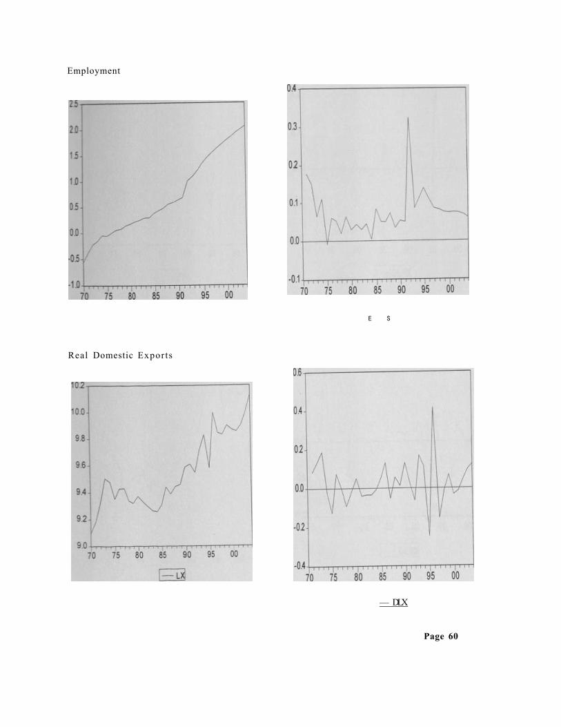
Employment
E S
Real Domestic Expor ts
— DLX
Page 60

— LPX
Real Manufactured Expor t s
1 — DLPX
— DLMX
Real Primary Exports
10JD,
Page 61

Real Imports
1 — LIM;
CUSUM Stability Test of Equation 4(b)
-10J , , , , , 1 95 96 97 98 99 00 01 02 03 04
' C U S U M 5% Significance I
CUSUM of Squares Stability Test of Equation
CUSUM of Squares, - _ 5%_Signi«cance
- DLIM
4(b)
Page 62

APPENDIX II: The Data
Domestic Manufactured Total GDP Exports Exports Imports
1970 10,432 2,061 179 2,841 1971 11,501 2,141 212 3,682 1972 13,172 2,557 224 3,679 1973 14,802 3,488 752 4.303 1974 17,926 4,577 876 7,384 1975 21,052 4,608 800 7,044 1976 25,562 6,708 985 8,140 1977 32,699 9,605 960 10,629 1978 35,601 7,399 967 13,223 1979 39,543 7,711 1.061 12,403 1980 44,648 9,753 1,343 19.181 1981 51.641 10,277 1.490 18,648 1982 60.987 10,915 1,356 18.006 1983 69,473 12,662 1,554 18,112 1984 77.524 15.096 1,715 21.944 1985 88.478 15.702 2,067 23,920 1986 102,299 19.159 2.286 26,758 1987 112.965 15.068 2,179 28,618 1988 129,612 18,354 2.720 35,303 1989 147.756 19,997 3,386 44.779 1990 168.455 24,647 4,151 50.913 1991 193,788 32,224 7,181 52,918 1992 228.050 34,162 6,730 59,097 1993 283,708 72.504 18,386 101.128 1994 338.065 83.414 26,919 115.080 1995 393,767 93.124 28,400 155,168 1996 449.621 113,926 30,499 168.486 1997 536,264 114,459 21,180 190.674 1998 596.539 114.445 26,510 197.789 1999 639.056 114.842 27,261 206.401 2000 685.436 119,764 26,883 247.804 2001 767.381 121.434 29,012 290.108 2002 849.988 131,394 34,930 257,710 2003 968,424 136,709 38,300 281.844 2004 1,080,328 159,063 38,700 364.205
NB: Values in Kshs millions at Current Prices, 2004 GDP estimated
U N I V E R S I T Y OF N A I R O B I
E M S T A F R I C A N A C O L L E C T I O M Page 63


