Air Force Institute of TechnologyAFIT Scholar
Theses and Dissertations Student Graduate Works
9-13-2012
Exploring the Dynamics and Modeling NationalBudget as a Supply Chain System: A Proposal forReengineering the Budgeting Process and forDeveloping a Management Flight SimulatorChristoforos Kalloniatis
Follow this and additional works at: https://scholar.afit.edu/etd
Part of the Operations and Supply Chain Management Commons
This Thesis is brought to you for free and open access by the Student Graduate Works at AFIT Scholar. It has been accepted for inclusion in Theses andDissertations by an authorized administrator of AFIT Scholar. For more information, please contact [email protected].
Recommended CitationKalloniatis, Christoforos, "Exploring the Dynamics and Modeling National Budget as a Supply Chain System: A Proposal forReengineering the Budgeting Process and for Developing a Management Flight Simulator" (2012). Theses and Dissertations. 1216.https://scholar.afit.edu/etd/1216

EXPLORING THE DYNAMICS AND MODELING NATIONAL BUDGET AS A SUPPLY CHAIN SYSTEM: A PROPOSAL FOR REENGINEERING THE
BUDGETING PROCESS AND FOR DEVELOPING A MANAGEMENT FLIGHT SIMULATOR
THESIS
Christoforos Kalloniatis, Captain, Hellenic Army
AFIT/LSCM/ENS/12-07
DEPARTMENT OF THE AIR FORCE
AIR UNIVERSITY
AIR FORCE INSTITUTE OF TECHNOLOGY
Wright-Patterson Air Force Base, Ohio
APPROVED FOR PUBLIC RELEASE, DISTRIBUTION UNLIMITED

The views expressed in this thesis are those of the author and do not reflect the official policy or position of the United States Air Force, Department of Defense, the United States Government, the Hellenic Army, the Ministry of National Defense of the Hellenic Republic, or the Hellenic Government.

AFIT/LSCM/ENS/12-07
EXPLORING THE DYNAMICS AND MODELING NATIONAL BUDGET AS A SUPPLY CHAIN SYSTEM: A PROPOSAL FOR REENGINEERING THE
BUDGETING PROCESS AND FOR DEVELOPING A MANAGEMENT FLIGHT SIMULATOR
THESIS
Presented to the Faculty
Department of Operational Sciences
Graduate School of Engineering and Management
Air Force Institute of Technology
Air University
Air Education and Training Command
In Partial Fulfillment of the Requirements for the
Degree of Master of Science in Supply Chain Management and Logistics
Christoforos Kalloniatis
Captain, Hellenic Army
September 2012
APPROVED FOR PUBLIC RELEASE, DISTRIBUTION UNLIMITED

AFIT/LSCM/ENS/12-07
EXPLORING THE DYNAMICS AND MODELING NATIONAL BUDGET AS A SUPPLY CHAIN SYSTEM: A PROPOSAL FOR REENGINEERING THE
BUDGETING PROCESS AND FOR DEVELOPING A MANAGEMENT FLIGHT SIMULATOR
Christoforos Kalloniatis Captain, Hellenic Army
Approved:
__________//Signed//_________________________ __31 Aug 2012_ Dr Cunningham William (Chairman) Date __________//Signed//_________________________ __31 Aug 2012_ Dr Cooper Martha (Member) Date

AFIT/LSCM/ENS/12-07
iv
Abstract
In the Science of Economics, there has been a debate about the optimal fiscal and
budgetary policy that should be implemented by governments. On the one side, the
advocates of the Keynesian Theory assert that in recession times governments should run
budgets with deficits, in order to stimulate the economy, while the supporters of the
Balanced Budget Theory, on the contrary, underscores the need to reduce and even
eliminate the budget deficits. However, previous experience shows that both theories can
fail to accomplish their goals, because they underestimate a very sensitive parameter:
national budgets are not just an estimate of revenues and receipts or a simple statement.
Rather, they are systems, the entities of which interact with each other and respond to any
event affecting their state. Even further, a national budget can be considered as a special
case of a supply chain system.
Within this framework, the present thesis seeks to introduce a new aspect in
budgeting. Specifically, the national budget is mapped as a supply chain and modeled as
a system. Thereafter, the research focuses on and explores the budget’s dynamics, which
are responsible for the failures experienced in the fiscal and budgetary policy and
concludes with a proposal for reengineering the budgeting process, according to the
postulates of the demand management process in a supply chain. Lastly, it underscores
the need to develop a Management Flight Simulator, which will reveal the dynamics of
national budgets, as the Beer Game does in the case of the supply chains, and that will act
as a learning tool for anyone interested in budgeting, supply chains or/ and public
economics.

AFIT/LSCM/ENS/12-07
v
To my wife and our daughter

vi
Acknowledgments
I would like to express my sincere appreciation to my thesis advisor, Dr William
Cunningham, for his guidance and support throughout the course of this thesis effort. The
insight and experience was certainly appreciated. I am also indebted to the reader of this
thesis, Dr Martha Cooper, for her mentoring, comments and help provided to me, in this
endeavor.
Moreover, I would like to thank Mrs. Robb, Director of the International Military
Students Office at AFIT and Lt Col Sharon Heilmann, for all their support and help.
I would like to express my sincere appreciation to my country and more
specifically to the Hellenic Army for this opportunity.
Lastly, and most importantly, my deepest gratitude and love to my wife and our
daughter for all their patience and understanding, and to my parents for their lifetime
support.
Christoforos Kalloniatis

vii
Table of Contents Page
Abstract .............................................................................................................................. iv
Acknowledgments.............................................................................................................. vi
Table of Contents .............................................................................................................. vii
List of Figures ......................................................................................................................x
List of Tables .................................................................................................................... xii
List of Equations .............................................................................................................. xiii
I. Introduction .....................................................................................................................1
General Issue ...................................................................................................................1 Problem Statement - Research Objectives ......................................................................2 Assumptions/Limitations ................................................................................................4 Preview ............................................................................................................................5
II. Literature Review ............................................................................................................6
National Budget ..............................................................................................................6 Budget Surplus – Deficits .......................................................................................... 8 Current Trends – Causes of Deficits ....................................................................... 13
Government/Public/National Debt ................................................................................16 The Traditional and the Ricardian View of Debt .................................................... 18 Debt: Dynamic not Static ........................................................................................ 20 Current Situation and trends ................................................................................... 21 Do Deficits and debt matter? .................................................................................. 22
Supply Chain Management ...........................................................................................38 Supply Chain Definition .......................................................................................... 38 Business Processes .................................................................................................. 42 Mapping Supply Chains .......................................................................................... 43
Systems - System Dynamics - Management Flight Simulators ....................................45 Systems- Models ...................................................................................................... 45 Simulation modeling - Management Flight Simulators .......................................... 50
The Beer Game .............................................................................................................52 Introduction to the Beer Game ................................................................................ 52 Rules 53 Results ..................................................................................................................... 55 Value - Lessons Learned from the Beer Game ........................................................ 56
III. Conceptual Model: Mapping a National Budget as a Supply Chain ...........................58

viii
Introduction ...................................................................................................................58 Mapping a National Budget as a Supply Chain ............................................................58
Supply Chain Tiers - Entities .................................................................................. 59 Links 63 Theoretical Justification of the Model..................................................................... 64 Practical Utility of the Model .................................................................................. 66
IV. Modeling and Exploring the Dynamics of the Budget Supply Chain as a System ....68
Budget as a System .......................................................................................................68 Entities ..........................................................................................................................68 Attributes .......................................................................................................................68 Activity ..........................................................................................................................68 Events ............................................................................................................................69 State of the system ........................................................................................................69 Flows .............................................................................................................................69 Classification of the Budget Model - System ...............................................................72 Dynamics of National Budgets: Theory and empirical evidence..................................76 Dynamics of the Budget System ...................................................................................76
Feedback Loops ....................................................................................................... 76 Time Delays ............................................................................................................. 84 Nonlinearities .......................................................................................................... 86 Stocks and Flows ..................................................................................................... 86
V. Reengineering the Budget Process: Utilizing the Supply Chain Demand Management Process in Budgeting..........................................................................................................87
Introduction ...................................................................................................................87 Reengineering the Budget Process: Utilizing Supply Chain Demand Management
Process in Budgeting ................................................................................................88 The Budget Team ..................................................................................................... 89 The Strategic Budget Process ................................................................................. 91 The Operational Budget Process ............................................................................ 96 The role of Information Technology to Reengineering Budget - Conclusions ........ 99
VI. The Budget Management Flight Simulator ...............................................................100
Introduction .................................................................................................................100 General Concept - Rules .............................................................................................101
VII. Conclusions and Recommendations .........................................................................104
Recommendations for Further Research .....................................................................105
Appendix A: OECD - Government deficit: Net lending/net borrowing as a percentage of GDP, surplus (+), deficit (-) .............................................................................................107

ix
Appendix B: General Government Gross Financial Liabilities as a percentage of GDP109
OECD Economic Outlook No. 91, OECD Economic Outlook: Statistics and Projections (database) .........................................................................................................................109
Vita. ..................................................................................................................................122

x
List of Figures Page Figure 1. The Global Debt Clock (The Economist) ............................................................ 3
Figure 2. The four stages of a National Budget .................................................................. 8
Figure 3. EU General government deficit/surplus (Percentage of GDP) 2011................. 14
Figure 4. U.S. Budget Deficit (1978 – 2016) .................................................................... 15
Figure 5. U.S. Gross Federal Debt and U.S. Gross Federal Debt as Percentage of the GDP
(1940-2017*) ............................................................................................................. 17
Figure 6. Deficit Effects .................................................................................................... 20
Figure 7. A simple Supply Chain (Hugos, 2003).............................................................. 39
Figure 8. Supply Chain Network for a Manufacturer ....................................................... 41
Figure 9. Types of Inter-Company Business Process Links ............................................. 44
Figure 10. Ways to study a system ................................................................................... 47
Figure 11. Beer Distribution Game Board ........................................................................ 55
Figure 12. Mapping National Budget as a Supply Chain ................................................. 60
Figure 13. Modeling Budget as a System ......................................................................... 75
Figure 14. Causal Loop Diagram Notation ....................................................................... 78
Figure 15. Feedback of the Keynesian Model .................................................................. 80
Figure 16. The Laffer Curve ............................................................................................. 81
Figure 17. CLD when tax rates increase ........................................................................... 83
Figure 18. CLD when tax rates increase ........................................................................... 84
Figure 19. The Strategic and Operational Sub Processes of Demand Management Process
................................................................................................................................... 90
Figure 20. Strategic Sub-Processes and Stages of the Budget .......................................... 91

xi
Figure 21. The Operational Sub Processes of Demand Management Process ................. 96
xii
List of Tables Page Table 1. Icons for Supply Chain Mapping ........................................................................ 64
Table 2. Symbols for Flow Diagrams ............................................................................... 72

xiii
List of Equations Page Equation 1. Budget Surplus/Deficit .................................................................................... 8
Equation 2. Government Budget Constraint ....................................................................... 9
Equation 3. Intertemporal Budget Constraint ................................................................... 33

-1-
I. Introduction
General Issue
In general terms, a Budget can be defined as an “estimate of revenue and
expenditure for a specified period” (Downes & Goodman, 2006). A special case of a
Budget is the National, Government, Public, or Federal Budget which the Oxford
Dictionary of Economics (Black, Hashimzade, & Myles, 2009) described as “a statement
of a government’s planned receipts and expenditures for some future period, normally a
year. This is usually accompanied by a statement of actual receipts and expenditures for
the previous period……The word budget originally meant the contents of a package; the
budget is so called because it brings all the government’s tax and spending plans together.
…”. A budget has a surplus when government’s receipts exceed the total expenditure or a
deficit when the expenses are greater than the revenue. In the case of equality between
the receipts and the expenditure, the budget is called balanced. Although before the Great
Depression, it was generally accepted that the budget should be balanced, Keynes
proposed that budget deficits may be desirable in periods of recession to stimulate the
economy (Stiglitz, 1986, p. 46). This approach as well as a number of other factors, such
as the governments’ failure to implement successfully their economic-tax policy and/or
the deviations between the actual and expected (budgeted) expenses - receipts in the
implementation stage and/or the inefficient use of the capital borrowed, led governments
to “run” budgets with deficits.
Budget deficits are financed mainly by borrowing (loans) and the total value of
government loans determines the country’s national or public debt (Stiglitz, 1988). A

-2-
deficit is not a static variable in the public debt’s formation; on the contrary, it is a
dynamic element, because of the interest that the governments have to pay to their
creditors or/and due to the need for “re-borrowing” in order to finance liabilities that
mature. The continuous governments’ trends to form and execute budgets with deficits
led to a situation where most of the countries (if not all) have to show at the present time
an, outstanding or not, amount of public dept.
Problem Statement - Research Objectives
Nowadays, sovereign debt has evolved into one of the most serious problems that
many governments have to solve and has been one of the main causes of the “crisis” that
the world economy faces. The current situation is highlighted by the debt crisis in the
Eurozone, the first, in history, US Federal Government’s downgrading concerning its
credit rating by Standard and Poor’s (5 August 2011) and the International Monetary
Fund’s financial help to even more countries that have been unable to finance their
budgets by borrowing the needed funds from the capital markets. Figure1 depicts
sovereign debt for 2012 and reveals that it is the U.S., Canada, Japan, and (some of) the
EU economies that are exposed to debt in higher levels than any other countries.
There is a plethora of “philosophies” and recommendations concerning the public
debt’s management. Some of these proposals involve the devaluation of the national
currency, stricter economic policies, austerity measures and plans, even defaults. On the
other hand, advocates of the Keynesian economics claim that the solution is to stimulate
the economy, even if that means even higher levels of debt and the maintenance of
running budgets with deficits.

-3-
Figure 1. The Global Debt Clock (The Economist)
Within this framework, the present thesis approaches the national budget as a
supply chain system and seeks to identify its dynamics which can lead both the
Keynesian theory and the Balanced-Budget approach, to fail in addressing the deficits
and public debt issue when implemented, and second to suggest a general framework of
budgeting, which could help face these failures. Specifically, a proposal is introduced for
reengineering the budget process, based on the supply chain demand management
process principles of operations and it is introduced the idea of developing a Budget
Management Flight Simulator, by utilizing systems dynamics, which will reveal the
-4-
complexity of budgets and the causes of fiscal policy failures, and will act as a learning
tool for anyone interested in public economics.
In order to achieve its research objectives, this study first approaches and maps
the national budget from a supply chain perspective, which depicts the relationships
between the budget’s entities as well as the structure of the fiscal and budget system. The
supply chain map is then used, as a basis for modeling a budget as a complex and
dynamic system. Thereafter, the budget’s dynamics are identified by utilizing systems
theory and the reasons that cause failures in the systems are acknowledged, in both the
Keynesian and the Balanced-Budget case. Finally, a general framework of forming,
implementing auditing budgets is initialized and, using the principles of systems
dynamics, a proposal for the development of a Budget Management Flight Simulator, that
will operate as a learning and educational tool, is introduced.
Assumptions/Limitations
The present thesis should not be considered as a research effort for optimal budget
policy or optimal level of debt, which are issues that have been extensively discussed in
the literature by economists, without reaching an agreement. Rather, it should be
considered as an effort to identify the reasons that budget policies fail to address the
deficits and public debt issues and as a proposal for a new framework for budgeting.
However, a review of the extensive literature concerning the budget deficits – public debt
issue was found necessary in order to model the national budget as a supply chain, to
show how economic thought evolved from balanced budgets to financing economy with
deficits and lastly to demonstrate the rationale which shaped the current status quo of

-5-
excessive sovereign debt and led many countries to run, especially in the later 20 years,
budgets with deficits.
Preview
The present chapter defines the problem and research objectives of this study, as
well as the assumptions and limitations that were made. Chapter II provides an extensive
review in the literature on the issues of budget deficits, public debt, supply chain, systems
theory and systems dynamics that are related to this research thesis. In Chapter III, the
national budget is mapped as a supply chain, and Chapter IV presents it as a system and
explores its dynamic elements and characteristics. Chapter V includes a proposal for
reengineering the national budget’s process and suggests the development of a
Management Flight Simulator. Finally, Chapter VI presents the conclusions of this thesis
and includes recommendations for further research.
-6-
II. Literature Review
National Budget
A budget, in general terms, is, as aforementioned, an “estimate of revenue and
expenditure for a specified period” (Downes & Goodman, 2006), or according to the IMF
Glossary of Selected Financial Terms (2006) as “a statement of the projected revenues,
proposed expenditures, and planned financing of any surplus or deficit of an entity,
especially government”. Research in this thesis focuses on government budgets which
usually cover a 12-month fiscal year period and may or may not match with a calendar
year. Stiglitz (1986, p. 47) parallelized them with the corporations’ income statements
and pointed out that they give a picture of the sources and the destinations of the money a
government collects and spends, respectively, adding that it is a measure of a
government’s cash flow, receipts and expenditure, too. However, a budget is not only a
descriptive statement of receipts and expenditure. Hackbart and Ramsey (2002, p.11)
“saw” budget as “a reflection of and the means by which the basic goals of the
government and society are achieved”, while Burkhead (1956) acknowledged a budget as
a “major weapon for instilling responsibility in the governmental structure” by bringing
public the government’s actions and destroying “the rule of invisible government”. In
parallel, Mussel (2009) stated that the budget is an instrument for governments to apply
their economic policy, a means of public relations, and that the purposes a budget serves
include the limitation and direction of governments’ activities and the effort to hold them
accountable. From another view, budgetary policies target an efficient allocation of
resources with the limitation of distributing the income fairly and to a stable

-7-
macroeconomic environment (OECD, 2012). Socially speaking, Caiden (1998) included
in the duties of government professionals (budget is formed and implemented by them)
the protection of the helpless, the service to the society by defending justice, the
environment’s protection, and the improvement of the health and the welfare of the
public.
Structurally, a budget is a cyclical process consisting of four stages (Mussel,
2009). The first is preparation, where an extended forecast takes place concerning the
revenue and the expenses for the year that the budget concerns. This procedure is usually
conducted by special government offices and departments, like the Office of
Management and Budget in the U.S. or the Ministry (Department) of Finance in other
countries. It must be mentioned that the agency responsible for preparing the budget
usually issues detailed instructions to all other government entities that are related to this
stage and asks the information sent by them to be in a certain format, because of the
amount of data gathered and time restrictions. The second stage is the approval of the
budget by a legislative body, like the Parliament or the Congress. After approval, the
budgets move to the implementation stage, which mainly involves collecting the revenues
and financing the activities of the budget. This stage contains all the actions which make
sure that the funds released by the government are spent for the purposes and the amounts
stated in the budget. Cash and debt management as well as essential adjustments in
budget plans are other activities that are associated with the implementation stage. Lastly,
the review stage consists of all the actions related to audits concerning the budget.

-8-
Figure 2. The four stages of a National Budget
Budget Surplus – Deficits
The budget surplus is defined as the excess of the revenues collected by the
government during a period of time (usually one year), over its total spending, while a
budget deficit is a negative surplus and indicates the level that the government’s revenues
fall short of its expenditure. The budget surplus is given by the following equation
(Dornbusch, Fisher, Startz, 1998):
Equation 1. Budget Surplus/Deficit
_ _ BS = TA − G – TR
__ _ where budget surplus is denoted by BS, TR are the government’s transfer payments , G is
the amount of government’s purchases of goods and services (spending) and TA is the
Preparation
Approval
Implementation
Review

-9-
revenue raised by taxes. When a deficit exists, government fills the gap between expenses
and receipts. There are mainly two potential sources of funds that can be used to finance
budget deficits. First, the government can borrow the funds needed and create debt by
issuing and selling bonds, which is a part of its fiscal policy and second, the deficit can be
financed by printing money, which is a means of monetary policy. This relation is shown
by the Government’s Budget Constraint (GBC), which is expressed with the following
equation (Kelton, 2011):
Equation 2. Government Budget Constraint
𝐺 + 𝑖𝐵𝑁𝑜𝑛−𝐺𝑜𝑣𝑡 = T + Δ𝐵𝑁𝑜𝑛−𝐺𝑜𝑣𝑡 +ΔM
where G is the non-interest spending of the government, 𝑖𝐵𝑁𝑜𝑛−𝐺𝑜𝑣𝑡 is the interest paid
due to the national debt that is held by non-governmental entities, T is the revenue raised
from taxation, ΔM denotes the change in the monetary base and finally Δ𝐵𝑁𝑜𝑛−𝐺𝑜𝑣𝑡 is the
change of the quantity of the government bonds held by the non-governmental entities.
The difference between spending G (outlays minus the interest) and taxes T (revenues) is
the primary deficit or surplus. What GBC mainly shows is that the budget deficit, which
equals spending (G) plus interest paid for bonds (𝑖𝐵𝑁𝑜𝑛−𝐺𝑜𝑣𝑡 ) minus tax receipts (T) is
covered either by borrowing (an increase in government’s bonds denoted by Δ𝐵𝑁𝑜𝑛−𝐺𝑜𝑣𝑡)
or by expanding the monetary base ΔM (printing money). The later phenomenon, namely
when the central banks print money to purchase a part of the government’s debt, is
known as “monetization” of deficits. Analyzing further the GBC equation we conclude

-10-
that a deficit in a national budget results in higher taxes and/or higher growth of money
and/or lower spending, in the future (Barth & Wells, 1999). It should be noted that some
economists (i.e. Dornbusch & Fischer, 1990) include in the GBC more sources of
revenue for the government (i.e. revenue from the privatization of companies that belong
to government), but creating debt and/or “monetization” of deficits are acknowledged as
the usual methods of financing budgets.
Budget deficits are mainly financed by the private sector (Mankiw 2010). In
particular, when needed, government issues bonds and sells them to investors in order to
cover the gap between expenditure and receipts. The creditors’ profit is the interest they
earn from purchasing the government’s bonds. However, nowadays, the private sector is
not the only borrowing source for governments. For countries that have been facing
severe problems with their public economics, the International Monetary Fund (IMF), an
organization with the participation of 188 countries that was established in order “to
foster global monetary cooperation, secure financial stability, facilitate international
trade, promote high employment and sustainable economic growth, and reduce poverty
around the world” (IMF, 2012), has been a source of financial funds, too. Additionally,
the recent world financial crisis triggered the establishment of the European Financial
Stability Facility (EFSF) by the euro area Member States, on 9 May 2010. EFSF, which
is a mechanism that helps countries participating in the Euro with financial problems,
(deficits, high debt), will be substituted by the European Stability Mechanism (ESM),
which is going to serve the same purposes. Lastly, but less usual, another way for a

-11-
government to finance its budget is by intergovernmental agreements for loans, under
which it borrows the funds needed from another country.
A second option for governments to finance budget deficits, besides borrowing is
just to monetize debt. However, this method has been widely criticized in the literature,
because of its effects to the economy, such as the increase of inflation. In an extreme
approach, Barth, Iden, and Russek (1986) considered monetization as “an indirect default
to the extent that the monetization leads to inflation which erodes the value of
outstanding debt”. Within this framework, Mankiw (2010, p.487) stated three reasons that
monetary policy is not used to address the problem of debt: First, he supported that
printing money is unnecessary as long as a government can sell debt, second central
banks have enough power to refuse to implement such policies and last but most
important, policymakers acknowledge that fiscal problems cannot be solved with
inflation. Worth mentioning that monetization of debt, namely the extent to which a
central bank finances the government’s deficit, depends on the level of its independence;
there are countries where governments have almost full authority over the country’s
central bank and others where central banks “enjoy” higher levels of independence.
Measuring Budget Deficit
The absolute value of the budget deficit (in currency units) cannot be considered
as a reliable measure of economic welfare, per se, for a number of reasons. In other
words, an economy with low or no deficits is not necessarily a prosperous economy. For
instance, underdeveloped countries or countries that have high national debt which
strengthens the possibility of a default or countries that experienced a default in the near

-12-
past and their economies have not recovered yet, usually lack the ability to run budgets
with deficits because of their inability to borrow financial funds from the world’s capital
and credit markets. Moreover, each country’s deficit in monetary units depends on a
number of factors i.e. the economy’s size - larger countries usually have higher needs for
funds to finance their budget. Under these conditions, the yardstick commonly used
nowadays to measure and to compare the budget deficit for a year is the ratio of the
deficit to the nominal GDP (both in monetary units) for this specific year. However, for
many economists even this index is insufficient and some of them (i.e. Rosen, 1992;
Mankiw, 2010) mentioned their concern about the traditional measures that are used to
express the magnitude of budget deficit and debt. Specifically, Mankiw (2010, p.472-46)
acknowledged four problems in the “traditional” way of measuring the deficit: The first
one is related to inflation in the sense that public debt is overstated by the amount of πD
where π is the inflation and D the nominal value of debt. The other ones have to do with
the fact that the value of capital assets and uncounted liabilities, as well as the business
cycles of the economy, are not taken into account, when the deficit is measured.
However, for the needs of this study we are going to use the nominal values of the budget
deficit and public debt as well as the ratio of these to the GDP.
Structurally, the budget deficit consists of the primary deficit and the interest
payments. The primary deficit is the difference between the government’s expenditure,
except interest payments, and the government’s revenue. In that sense, primary deficit
represents the burden that a government creates and the interest payments are the legacy
of past economic policies (Dornbusch et al., 1998, p.477). As it can be inferred, the

-13-
relation between primary deficit and interest payments is substantial for the government’s
fiscal policy. The higher the debt, the higher the interest (interest payments which appear
in the budget as an outlay) that should be paid each year, and consequently the less
available revenue for the government.
Current Trends – Causes of Deficits
As shown Appendix A, which presents the evolution of the OECD governments’
surpluses/deficits during the last 6 years and 1 in future and as mentioned in the OECD
Factbook 2011-2012: Economic, Environmental and Social Statistics “there is a big
variation in the shares of expenditure and revenues in the GDP across the OE CD
countries and over time”. In 2011 Ireland’s deficit was 13% of its GDP, Estonia had 1%
deficit/surplus, and Norway showed a surplus of 13.6%. In addition, there is difference in
deficit/surplus over the years for all countries. For example, the rule for the US Federal
Government was to run budget surpluses with the exception of wartime (Dornbusch et al.,
1998). Though, now deficits became the rule in the United States. Especially, after the
year 2008, when the global economic recession started, the United States experienced a
situation where budget deficits increased sharply. Specifically, the deficit of the US
Federal Government reached the amount of approximately $ 1.4 trillion in 2009 (Figure
4).
A similar trend, during the financial crisis the world economy has been facing
since 2008, is observed in many other western economies, too. For example, according to
Eurostat, the governments’ budget deficits in the Euro area as a percentage of the GDP
rose from 0.7% in 2007 to 6.4% in 2009 and in 2011 many of the member-countries did

-14-
not manage to achieve the 3% goal-deficit implied by the Stability and Growth Pact
(SGP). In Japan a similar substantial deficit increase took place. Nowadays, we
experience a period where the first signs of recovering from the crisis are expected,
although some countries continue to face serious fiscal problems and have severe deficits
in their budgets.
Figure 3. EU General government deficit/surplus (Percentage of GDP) 2011
The increase of deficits during the latest years is attributed to the world’s
economic recession and financial crisis which especially western economies have been
experiencing since 2008: Governments, loyal to the Keynesian theory, increased
spending in their effort to revitalize the economy and avoid the “death spiral” of
recession. Moreover, several studies (Gale & Orszag, 2003; Mankiw, 2010) underscored

-15-
that the main causes of budget deficits in the U.S. are the parameter of aging population
and the rising cost of healthcare. Earlier, Apostolides (1999) had argued that these two
parameters (health care and public pension system financial needs) will affect deficits of
the OECD member-countries, if left without attention. He also indicated that the increase
of budget deficits in these countries by the fact that government expenses have been
growing faster than revenues - Tanner (2011) underlined that the real budget problem of
the U.S. is a spending problem rather than a revenue issue, too- and attributed this
phenomenon to a number of reasons: The change of the government’s role in the
economy, the different attitude over the budget deficits (Keynesian theory of deficits
prevailed in many cases over running balanced budgets), the increase of social spending,
demographic reasons, structural unemployment - inflation and to the economic activity’s
slowdown that took place in many countries.
Figure 4. U.S. Budget Deficit (1978 – 2016)
Source: Office of Management and Budget, executive Office of the President (Last updated Feb 21 2012)

-16-
Government/Public/National Debt
Eurostat defines the government, national or public debt as “the sum of external
obligations (debts) of the government and public sector agencies”. From a different view,
debt is the accumulation of past borrowing (Mankiw, 2010, p.467) and it is the
“aftermath” of running budgets with deficits or as Stiglitz stated (1986, p.42), defining
comprehensively the relation between budget deficit and national debt, “deficit is the
additional value of the debt incurred by the government in any year”. National debt is
referred in the literature either as the Government Gross Debt which equals all of a
government’s financial liabilities, (mainly government bills and bonds) or as the
Government Net Debt which is defined as the difference between the sum of all the
government’s liabilities and the value of all government’s financial assets (OECD
Glossary of Statistical Terms, 2012). Relative to its source, government debt is separated
to internal and external debt. Internal debt consists of the government’s liabilities to
lenders within the country, and as characteristically stated by Adam Smith (1776) in this
case “it is the right hand which pays the left”. On the other hand, gross external debt, at
any given time, is “the outstanding amount of those actual current, and not contingent,
liabilities that require payment(s) of interest and/or principal by the debtor at some
point(s) in the future and that are owed to nonresidents by residents of an economy (IMF,
2003)”. Similarly with the case of the budget deficit, the “common” metric used for
measuring one country’s debt in relation with the size of its economy is the debt-income
ratio for a year, which is the value of the total debt divided by the country’s nominal GDP

-17-
for this year, though, Eisner and Pieper (1984) supported the opinion that official
measures of debt and deficits should take into account the government’s assets, either
financial or not, of the period that was used as the basis of reporting the deficit/debt.
Figure 5. U.S. Gross Federal Debt and U.S. Gross Federal Debt as Percentage of the
GDP (1940-2017*) Source: The White House Office of Management and Budget
In this point, it is important to emphasize the difference between the nominal
gross debt and the Debt/GDP ratio, for measuring the public debt’s magnitude. Figure 5
shows the U.S. Gross Federal Debt and the U.S. Gross Federal Debt as percentage of
GDP. As it can be easily implied, the behavior of the two indexes is totally different. The
0 5
10 15 20 25
1940
19
46
1952
19
58
1964
19
70
1976
19
81
1987
19
93
1999
20
05
2011
20
17 …
U.S. Gross Federal Debt in Trillions of U.S. Dollars
Gross Federal Debt
0
50
100
150
1940
19
47
1954
19
61
1968
19
75
1981
19
88
1995
20
02
2009
20
16 …
U.S. Gross Federal Debt as Percentage of
GDP
Gross Federal Debt as Percentage of GDP

-18-
Gross Federal Debt behavior can be considered as exponential, while when graphed as a
percentage of the GDP its mode is dissimilar and it shows oscillations.
The Traditional and the Ricardian View of Debt
In the literature, there are mainly two points to view on public debt in terms of its
consequences to the economy: the traditional or conventional and the Ricardian view.
The traditional or conventional view suggests that a deficit in the budget and
consequently an increase in the public debt will lead to a “domino” of economic
phenomena. According to Mankiw (2010), the traditional view implies that in the short
term, government spending on consumption will be increased and this will result in the
rise of output and employment, which in turn, will increase interest rates and inflation.
Consequently, investment will be reduced, the value of the country’s currency will
strengthen and the domestic economy will lose in competitiveness. Furthermore, in the
long run, although the overall effect on welfare is hard to judge, there is a general notion
that the current generation would benefit at the expense of future generations, in the sense
that it (the current generation) “enjoys” higher rates of employment and consumption and
imposes a burden to society that has to be paid in the future.
In contrast, the Ricardian equivalence hypothesis proposed by Barro (1974 &
1989), assumes that taxpayers will not increase their consumption in the case of a tax-cut
financed by an increase in debt. On the contrary, as tax-payers expect a future increase in
taxes in order to pay the debt caused by the tax-cut to be offset, they increase their
savings, responsively, in order to face this situation in the future (Barro, 1974).
Consequently, none of the predictions made due to the traditional view will come true.

-19-
The Ricardian Equivalence Theorem has been criticized in the literature for its accuracy.
For example, based on previous studies (Bernheim, 1987; Ball & Mankiw, 1995), Barth
and Wells (1999) declared that “The view that deficits will have no effect on economic
activity is disputed by both Keynesians and fiscal conservatives, who argue that it is
based upon questionable assumptions (Bernheim, 1987). Regardless of the merit of the
assumptions, substantial empirical evidence exists that fail to support the Ricardian
Equivalence theorem.” Similarly, other economists reject this view because they believe
that the prospect of future taxes does not influence present consumption because
taxpayers do not have the assumed knowledge and foresight of the government’s acts and
because of the borrowing constraints that people are subject to, by the banks (Mankiw,
2010). Gale and Orszag (2003), depicted the Ricardian equivalence theorem as well as
the othe different views on deficits comprehensively, as Figure 5 shows.
Elmendorf and Mankiw (1999) argued in a research paper that “… the idea of
Ricardian equivalence has been extraordinary important within the academic debate over
government debt”. In particular, the Ricardian equivalence, although theoretically correct,
is too “utopian” to be true in the real world. Despite the fact that potentially there will be
individuals that will follow what the Ricardian approach implies (increase savings
because they wait for a tax increase in the future), there will always be such a part of the
population who will behave according to the Traditional view (increase spending for
consumption), that will trigger all the forecasted economic phenomena.

-20-
Figure 6. Deficit Effects Source: Economic Effects of Sustained Budget Deficits
Gale, William D; Orszag, Peter R; National Tax Journal; Sep 2003; 56, 3; ABI/INFORM Research
Debt: Dynamic not Static
Governments do not borrow only to finance their current deficits, though an
outstanding share of the funds borrowed is used in order for previous debt to be paid back
to creditors in the form of principal debt or interest. So, the nature of budget deficits and
the public debt is not static, but dynamic due to the interest that the governments have to
pay to their creditors. Specifically, budget deficits increase government debt. Higher debt
demands higher yearly payments in interest or in principal debt. Taken into account that
each year’s debt payments are included in the budget as an expense, there is a risk that,

-21-
under some circumstances, the continuous raise of debt will continuously decrease the
funds available for the government budget revenue, until a point where the amount of
money needed to satisfy debt needs will be so high that government will be unable to
finance its operations with the remaining revenue and finally default. In other words,
there will be a point in the future that the debt will be unsustainable, mainly due to the
high demand of financial funds to repay debt, either principal or interest.
Current Situation and trends
High level of debt was traditionally considered as a usual phenomenon only in
periods of depression or war time (Elmendorf and Mankiw, 1999). However, government
debt has shown an increase since the 1980s, especially in the large western economies,
and has evolved nowadays into an important financial-economic issue. Indicatively, the
debt of the U.S. Federal Government increased from 26% of the country’s GDP in 1980
to 98.3% in 2010, exceeded the “symbolic tipping point” of 100% in 2011 and it is
expected to exceed the level of 108% of GDP in 2012, according to OECD Data
(Appendix B). This evolution led to the first in history credit rating downgrade of the
American economy by Standard and Poor’s in 2011. Similarly, Eurozone in general, and
especially some of the countries that participate in this economic and monetary union
(EMU), experienced an unprecedented sovereign debt crisis, while Japan’s debt is
expected to reach the 222.6% of the country’s GDP in 2013.
Considering the undesirable effects of debt on the economy and society, some
States of the U.S. have passed laws that require local governments to run balanced
budgets. Specifically, all states except one required a kind of budget balance (Yilin Hou,

-22-
Daniel Smith, 2006). As the debt of the Federal Government has recently increased
substantially, a debate is taking place nowadays whether a same clause should be applied
for Federal budget, too. Although, consensus has not been achieved yet, in the past the
U.S. government voted for legislation related to budget deficits and the amount of debt
(i.e. Balanced Budget and Emergency Deficit Reduction known as Gramm / Rudman /
Hollings Act, 1985). The EU established the Stability and Growth Pact (SGP), which is a
framework to safeguard public finances within the economic and monetary union. In its
dissuasive part, SGP contains the Excessive Deficit Procedure (EDP), which is triggered
when one country’s deficit reaches the level of 3% of GDP. In that case, the EU provides
at first the country with recommendations for how to address the problem. In case of non-
compliance further action against the country is taken, including for euro-area countries
the potential of imposing sanctions. Moreover, the Treaty on Stability, Coordination and
Governance in the Economic and Monetary Union, which was signed on 2 March 2012
by the EU Member Countries with the exception of the United Kingdom and the Czech
Republic and is expected to enter into force on 1 January 2013, implies a stricter
framework concerning budgetary policy. In particular, participating member-countries
agreed to run budgets, from 2013, either balanced or with surpluses.
Do Deficits and debt matter?
As aforementioned, balanced budgets was the prevailing strategy, until Keynes developed
his theory according to which deficits may be desirable in periods of recession, so as to
stimulate the economy (Stiglitz, 1986). Since then, there has been a plethora of research
studies, newspaper articles and journal papers that address this issue. On the one hand

-23-
there are economists who support budgets to be balanced, while on the other hand we
find advocates of the opinion that deficits are beneficial for the economy under certain
conditions. The debate of these two schools of economic thought seems to have started on
October 1932. In particular, Keynes and five more economists (MacGregor, Pigou,
Layton, Salter and Stamp) sent a letter to London Times which was published on 17
October 1932. This letter is thought to be a cornerstone to Keynesian economics, as it
underscored that “the public interest in present conditions does not point towards private
economy; to spend less money than we should like to do is not patriotic.” (MacGregor et
al., 1932). In order to support their point of view about the need of spending, the authors
of the article used a characteristic example, according to which “If the citizens of a town
wish to build a swimming-bath, or a library, or a museum, they will not, by refraining
from doing this, promote a wider national interest. They will be “martyrs by mistake,”
and in their martyrdom, will be injuring other as well as themselves. Through their
misdirected good will the mounting wove of unemployment will be lifted still higher.”
The answer came two days later by Hayek and three other professors (Gregory, Plant,
Robbins), who, among others, disagreed with the Keynesian view of budget deficits.
Specifically, they argued that high levels of public debt results in “frictions and obstacles
to readjustment very much greater than the frictions and obstacles imposed by the
existence of private debt” and answered to Keynes et al. (1932) example by stating that
“… we cannot agree with the signatories of the letter that this is a time for new municipal
swimming baths…”. The right behavior for governments was according to Hayek et al.
(1932) “… to abolish those restrictions on trade and the free movement of capital

-24-
(including restrictions on new issues) …” Another interesting approach about deficits is
the one stated by the Austrian School of economic thought, according to which:
“It is important to point out that Austrians do not argue that fiscal restraint or
"austerity" will bring about economic growth (America's Great
Depression, Murray Rothbard, 1963). Rather, they argue that all attempts by
central governments to prop up asset prices, bail out insolvent banks, or
"stimulate" the economy with deficit spending will only make the misallocations
and malinvestments worse, prolonging the depression and adjustment necessary to
return to stable growth1. Austrians argue the policy error rests in the
government's (and central bank's) weakness or negligence in allowing the "false"
credit-fueled boom to begin in the first place, not in having it end with fiscal and
monetary ‘austerity’”. (Wikipedia, 2012).
It should be noted that the Austrian School of economics has gained in popularity lately,
because it had predicted, in some way, the financial crisis of 2007-2008. Specifically,
according to the Austrian School of economics low interest rates trigger the amplification
of public debt, creating investment bubbles, which, in turn, when they burst cause a crisis.
This is more or less what happened in 2007 – 2008 (Financial Times Lexicon, 2012).
Although, since this debate, there has never been agreement about the optimal
deficits-debt issue among economists, the Keynesian theory started to gain approval by
an increasing number of economists and policy- makers throughout the years. It is
“convenient” for governments to run budgets with deficits, as they have in their disposal

-25-
more resources to apply their policies. Though, during the last years, when the first
problems started to appear due to deficits and debt, the balanced-budget approach seems
to gain more and more advocates.
Adam Smith devoted a whole chapter in his book “The Wealth of Nations”, which
is thought to be a cornerstone in the science of Economics, discussing the topic of public
debts (Book V, Chapter III). Particularly, Smith (1776) warned that the enormous
accumulated public debt oppressed at that time in all the great nations of Europe could
become a factor of ruining them in the long-run. He also expressed the opinion that “The
more the public debts may have been accumulated, the more necessary it may have
become to study to reduce them, the more dangerous, the more ruinous it may be to
misapply any part of the sinking fund”, which reveals his high concern about debt.
Furthermore, a powerful argument expressed by the opponents of budget deficits
and public debt is that current deficits are transferred from present to future (Stiglitz,
1986; Aliabadi et al., 2011; Laffargue, 2009; Barro 1974) and some of them introduce the
moral issue of how fair this shift is between generations. Specifically, Laffargue (2009)
argued for governments which “finance the costs of their transfers to the living by
increasing public debt recklessly”, that they increase taxes paid by consumers in order to
finance debt, which leads future generations to a process of “immiserisation” and
emphasized the fact that “Governments make their decisions without putting weight on
the welfare of future generations”. Moreover, Mankiw (2010) acknowledged that in the
short run, government borrowing resulted from a tax-cut would raise demand, output and
employment as well as the interest rates. Consequently, investment would be reduced,
-26-
capital flow from abroad would increase and finally economy would lose in
competitiveness, through a currency appreciation. In the long run, such a policy would
lead to smaller capital stock and to a higher debt level. Mankiw also argued that “simply
increasing the budget deficit is not feasible” and underlined the political impact of a high
debt rate: First, an increase in foreign borrowing will possibly have negative political
impacts as political power is related to whether a country is a debtor or creditor in the
world’s economy. To support this view he used Ben Friedman’s words in the book “Day
of Reckoning”:
World power and influence have historically accrued to creditor countries. It is
not coincidental that America emerged as a world power simultaneously with our
transition from a debtor nation … to a creditor supplying investment capital to the
rest of the world [Friedman, 1988 - quoted in Mankiw (2010)].
Second, Mankiw argued that a high level of debt increases the potential of a
default. Debt default as defined by the International Monetary Fund (2003) is the “failure
to meet a debt obligation payment, either principal or interest. A payment that is overdue
or in arrears is technically ‘in default,’ since by virtue of nonpayment the borrower has
failed to abide by the terms and conditions of the debt obligation. In practice, the point at
which a debt obligation is considered ‘in default’ will vary.” As a government continues
to run budgets with deficits and debt increases, credit markets become worried about the
potential that the country will not be able to repay its debts in the future. The level of
concern is usually depicted in the interest rate (bond yields) by which a country borrows
from the investors in the world’s financial markets. The norm is that “weaker” economies

-27-
or/and countries with high debt usually pay higher interest rates. As the level of debt
increases, investors gradually lose their confidence that they are going to be paid back the
money they lent and the interest rate increases, until the point where bonds cannot be sold
to markets, due to the investors’ unwillingness to buy them or until the moment that the
interest rate that is required to be paid by the country is “prohibitive” for the future
sustainability of its debt. It is then that the country defaults, because it fails to pay a
mature debt obligation. Worth mentioning at this point that creditors’ fear of a default is a
“sensitive” parameter as governments/countries/sovereigns are not subject to the same
sanctions that a company faces when bankrupted. Actually “There are no international
statutes to deal with a sovereign debt default…” (Olivares-Caminal, 2010). In particular,
when a corporation goes bankrupt, usually it is the court that intervenes in order for its
assets to be liquidated and/or its management to be substituted. On the contrary, when a
country defaults there are no practical sanctions to be imposed as in the case of an
enterprise, because litigation is a time consuming and costly process, which can be
proved as a “futile and hopeless labour” (Olivares-Caminal, 2010). However, previous
experience of defaults (i.e. Argentina) shows that its consequences to the economy and
society are severe. As stated by Kottlikoff and Burns (2005) in the prologue of their book
“The Coming Generational Storm: What You Need to Know about America's Economic
Future” [quoted in Kelton (2011)]:
History is replete with examples of what happens when countries can’t pay their
bills. They raise taxes to exorbitant levels, default on their explicit or implicit
obligations, and begin printing money like mad. This triggers inflation, drives

-28-
interest rates through the roof, and sends exchange rates down the tubes.
Businesses go belly up, and banks shut their doors. The result is financial and
economic meltdown (2004, xxiii).
So, in case of a default, the value of the domestic currency collapses, interest rates and
inflation increase sharply, investors lose their confidence and avoid-refuse to lend their
money to the defaulted country for a long period of time, imports become difficult and
the government has no choice but to rely exclusively on the tax-revenue to implement its
fiscal policy.
Other consequences of high government debt and budget deficits are the reduction
in economic performance by crowding out private investment and the decrease of
national income (Apostolides, 1999). Specifically, when foreign ownership of domestic
bonds, real estate or equity increases there is a flow of income in the form of interest or
profit abroad, which causes the reduction of the national income. Gale and Orszag (2003)
attributed the decrease of national income to sustained deficits, too. In particular, they
stated that deficits cause a decrease in national saving, future national income and
consequently future living standards (other factors constant), no matter if the interest rates
increase or not and regardless of the magnitude of the foreign capital flows. Furthermore,
Elmendorf and Mankiw (1999) underscored a number of other effects of debt over the
economy, including “the deadweight loss of the taxes needed to service that debt”, the
reduction of government’s flexibility to apply its fiscal policy and the increase in
vulnerability to a crisis of international confidence. Moreover, they argued that debt can
affect monetary policy. For example, high debt can trigger an increase in money supply

-29-
when there is difficulty for the government to borrow in order to finance its deficits,
which in turn is the “classical explanation for hyperinflation”. In parallel, Stiglitz (1986)
mentioned that, indeed, there is a concern about the issue that deficits result in inflation
and higher interest rates. Though, it should be mentioned for the deficit-inflation
relationship that Abizadeh and Yousefi, (1999) described a situation in the literature
where no consensus existed among economists on this issue and stated that the empirical
evidence for this subject is contradictory. In addition, Aliabadi et al. (2011) investigated
the relation between first, government spending and unemployment, and second, between
government spending and the Consumer Price Index (CPI) and concluded that there is no
significant association among them. However, it should be stated that CPI has been
calculated differently over the years (www.shadowstats.com). Lastly, Bowles (2012)
acknowledged deficits of the Federal Government as the most important threat of the U.S.
national security that should be faced neither entirely with raising taxes nor just with cuts;
instead the solution should include an economic growth parameter, too.
The Congressional Budget Office (CBO) “warns” that debt’s negative
consequences are not restricted to the output area. On the contrary, rising debt would lead
to higher interest payments for that debt annually, which would result in higher taxation
or in a government’s benefit and services reduction, or in a combination of the two.
Moreover, it would reduce the policymakers’ ability to face unexpected events such as a
financial crisis or an economic downturn. Finally, the CBO mentions that rising debt
would make a sudden fiscal crisis more possible, during which the government would not
be able to borrow at rates it can afford.

-30-
On the contrary, the advocates of deficits and debt stress a number of reasons that
dictate the implementation of non-balanced budgets. Generally, using the Keynesian
theory as a basis for their beliefs, they argue that deficits leverage the economy and pay
back the money borrowed in terms of increasing the national income (GDP). Historically,
it was Keynes in his book “The General Theory of Employment, Interest and Money”
(1936) that introduced the theory which implies that in recession periods during which
economy suffers from low employment rates, government should increase its spending by
running budgets with deficits, in order the recession to be confronted and the employment
rates to raise. The debt created during recession is to be paid when the economy recovers
either by increasing taxes or/and by reducing expenses. He writes characteristically:
“If the Treasury were to fill old bottles with banknotes, bury them at suitable
depths in disused coalmines which are then filled up to the surface with town rubbish,
and leave it to private enterprise on well-tried principles of laissez-faire to dig the notes
up again (the right to do so being obtained, of course, by tendering for leases of the note-
bearing territory), there need be no more unemployment and, with the help of the
repercussions, the real income of the community, and its capital wealth also, would
probably become a good deal greater than it actually is. It would, indeed, be more
sensible to build houses and the like; but if there are political and practical difficulties in
the way of this, the above would be better than nothing." (Chapter 10)
He also highlighted that “…It is for this reason that a change-over from a policy of
Government borrowing to the opposite policy of providing sinking funds (or vice versa)
-31-
is capable of causing a severe contraction (or marked expansion) of effective demand”
(Chapter 8).
Likewise, Mankiw (2010, p.486) stated that deficits or surpluses may at times
help the economy to stabilize. Specifically, in recession periods, government tax-revenue
declines due to the decrease in economic activity. In that case, the implementation of a
strict fiscal policy with balanced budgets will result in further recession, while an
increase in public spending through running a deficit will revitalize the economy.
Economists that support this view, declare that if governments insist to apply balanced
budgets and austerity measures in recession periods, the economy will be led to a “death
spiral” of continuous recession. The choice between austerity measures to balance the
budget and finance growth with further deficits has evolved nowadays into a debate
between economists and policy makers throughout the EU, during the sovereign crisis in
the Euro-area. Other reasons, according to Mankiw, that in some cases justify deficits are
the needs for “tax smoothing” and the needs to redistribute taxes among generations,
namely move taxes from current to future generations. Correspondingly, Alesina and
Tabellini (1990) mentioned that budget deficit and national debt serve a twofold purpose:
First, they are used for “redistributing income over time and across generations” and
second, “they serve as a means of minimizing the deadweight losses of taxation
associated with the provision of public goods and services”. Moreover, Galbraith (2010)
criticized the supporters of reducing deficits declaring that a program to reduce deficits
would destroy the economy, mentioning that “To cut current deficits without first
rebuilding the economic engine of the private credit system is a sure path to stagnation, to

-32-
a double-dip recession - even to a second Great Depression”. He also provided arguments
that for governments which keep control over their currency, the risk for nonpayment and
consequently default, does not exist, and he expressed the opinion that debt is not a
burden transferred to future generations and interest not a threat to the country’s
solvency. Kelton (2011, p.60) added to this argument that in countries like the U.S.,
deficits showed a temptation to cause a reduction of interest rates, favoring the view that
interest rate is a “policy variable” the nominal value of which can be set by the Federal
Reserve, no matter the level of deficit (p.61). Kelton also doubted about the predictions of
the dominant macroeconomic models that high levels of deficits and debt will increase
inflation and interest rates in the long-term, as well as cause the reduction of growth. In
order to support this point, Kelton used the historical paradigms of the U.S. and U.K.
economies, mentioned by Levy and Thiruvadanthi (2010), according to which although
right after World War II there was a high ratio of public debt, the inflation during the
following decade was kept at a low level. It was also mentioned, in this research paper,
that high public debt periods have preceded high economic growth. Moreover, Kelton
(2011) used the example of Japan in order to support that deficits and high debt is not a
cause of higher taxes. Specifically, it was highlighted that according to data, despite
Japan’s high level of debt (the higher in OECD members that is expected to exceed the
226% of the GDP in 2013) taxes imposed in this country continue to be among the lowest
of the developed countries. In one of the most “extreme” versions of support to deficits,
some economists, known as supply-siders argue that a tax-cut and consequently a deficit
can be “self-financed” in the sense that the increase in aggregate supply will be so high

-33-
that it can offset any revenue losses for the government (caused by the decrease in
taxation) (Mankiw, 2010). Based on this assumption, some supply-siders believe that a
deficit is not an important issue in fiscal policy and reject the hypothesis that interest rates
and inflation is increased by deficits (Yousefi, 1999).
Further reference to the literature about the issue of deficits and debt goes beyond
the scope of this Thesis. The main conclusion is that there is no agreement between
economists about the measurement or/and the effects of the government debt or about the
correct budget policy (Mankiw, 2010, p.490); there is an open debate about this issue not
only between economists but among policy makers, too [i.e. disagreement between
Republicans and Democrats in 2011 (U.S.) about the debt “ceiling” and among European
politicians about the right strategy so as to overcome recession (austerity vs deficits to
finance growth)]. Aliabadi et al. (2011) mentioned, budget deficit and public debt has
been a field of research and controversies. Moreover, Alexander Hamilton mentioned
that “a national debt, if it is not excessive, will be to us a national blessing”, while James
Madison’s believed that “a public debt is a public curse".
By another view, running deficits in national budgets should be examined on a
case-by-case basis according to the intertemporal budget constraint which is given by the
following equation (Kelton, 2011 following Blanchard, 1990):
Equation 3. Intertemporal Budget Constraint
𝛥 (𝐵𝑡/ 𝑌𝑡 ) = (r – g) 𝐵𝑡−1𝑌𝑡−1
+ (𝐺𝑡− 𝑇𝑡 )𝑌𝑡

-34-
where 𝐵𝑡/ 𝑌𝑡 is the public debt ratio, r is the real interest rate, g denotes the output
growth, Gt is the non-interest government spending, T the tax receipts, B the
government’s debt and Y the output. The(𝐺𝑡− 𝑇𝑡 )𝑌𝑡
part of the equation depicts the primary
deficit to output while the fraction 𝐵𝑡−1𝑌𝑡−1
denotes the “heritage” of past economic policies
applied. The intertemporal budget constraint shows that the ratio of the nominal debt to
output (𝐵𝑡/ 𝑌𝑡) can decline even if the primary deficit (𝐺𝑡 − 𝑇𝑡 ) is increasing in absolute
value, given that the value of the output growth g is greater than the real interest rate r.
Economists’ disagreement about the significance of debt is based on the relation between
interest rates, debt and growth. Advocates of deficits argue that growth can outpace real
interest at a rate where the ratio of debt to output can be reduced, while on the other hand,
“the conventional theory tends to dismiss this possibility” (Kelton, 2011, p.59). So,
according to this theory, government borrowing and deficits’ utility is a matter of growth.
If borrowed funds are invested productively so as the rate of national income growth is
stimulated and outpace the rate of interest (which may be increased by adding the (new)
borrowed funds to the country’s economy), then borrowing is beneficial for the country:
Economy grows and the public debt ratio decreases. For example, if a government
decides for a tax-cut for companies through creating a budget deficit, then this action will
be beneficial only if the amount saved from taxation is invested in activities that will
grow national income substantially. On the contrary, if funds are used for
“counterproductive” activities (i.e. spending on imported consumer goods) then national

-35-
income will not be raised and borrowing will just result in a higher public debt ratio.
Barth, Iden amd Russek (1986) presented this point of view in detail:
This brief discussion indicates that the disagreement over the economic
consequences of federal deficits seems to hinge on whether or not the federal debt
is net wealth. In this regard it has been argued that, if the rate of interest is less
than the rate of growth in the economy, then federal debt is unambiguously net
wealth. The reason is that in this case higher future taxes are not needed to service
the debt – economic growth will be sufficient to run deficits indefinitely without
exceeding the taxing capacity of the economy. If, however, the rate of interest
exceeds the growth rate, then the status of federal debt is ambiguous. It will be net
wealth only to the extent that current generations do not fully discount the
increase in future tax liability necessary to service the debt, which in this case
cannot be serviced solely with revenues generated by economic growth.
… A potential problem arises, however, if one assumes that the rate of interest
exceeds the growth rate. This is the problem of instability – unbounded growth of
the federal debt relative to GNP. If the rate of interest exceeds the growth rate and
there is a primary deficit (i.e. federal government expenditures net of interest
payments exceed tax receipts), then federal debt will continually grow more
rapidly than the economy. (p. 28)

-36-
Barth et al. (1986) continued their analysis by mentioning that if the situation of
instability continues, government will eventually either default or monetize its deficits,
which as aforementioned can be considered as an indirect default.
Within this framework, the increasing evolution of the debt/GDP ratio,
experienced especially in the western economies since 1980, can be attributed to a
continuing condition of instability that these economies faced. In other words, countries
used funds borrowed to finance deficits “inefficiently” in the sense that income was not
raised substantially enough, so as the government loans to be paid back. Therefore, debt
has been accumulating and tax revenue has not followed its pace of increase. As a result,
in some countries debt has risen to or close to unsustainable levels. Moreover, our
perception is that the high debt level of some countries is associated with choices
concerning the economic policies. In particular, the theory which supports deficits in
national budgets during recession periods also implies that deficits should be paid back
when the economy recovers. Data reveals that this is not what exactly happened since
1980. Even in boom economic periods budgets in western economies continued to raise
their debt and deficits, somewhat unreasonably. Adam Smith (1776) in his approach
mentioned about the public debt that when an event occurs in peacetime which needs to
be financed by the government, it is more convenient that this expense to be financed by
adding to debt (borrowing) rather by imposing new taxes that are immediately identified
by tax-payers and people complain about them.
The current situation is highlighted by the debt crisis in the Euro-zone, the first, in
history, US Federal Government’s downgrading concerning its credit rating by Standard
-37-
and Poor’s (5 August 2011) and the International Monetary Fund’s financial help to even
more countries that have been unable to finance their budgets. No matter what the causes
of running budgets with deficits and accumulating debts were, nowadays there are many
countries which are close to or have crossed the “red line” of their debt sustainability
limit and must act now in order to improve the “health” of their budgets and their national
accounts. Future forecasts and trends for debt and deficits call for immediate action now.
Both of these views are justified widely in recent literature by academics, policy makers
and economists. Douglas W. Elmendorf, Director of the Congressional Budget Office, in
response to a request from House Budget Committee Chairman Paul Ryan, highlighted
the need for policy changes so as the U.S. budget deficits would be reduced. Specifically,
he stated that:
“The explosive path of federal debt that the Congressional Budget Office (CBO)
projects under what many observers would view as current policies underscores
the need for policy changes to put the nation on a sustainable course. The aging of
the population and rising costs for health care will push spending for Social
Security, Medicare, Medicaid, and other federal health care programs
considerably higher as a percentage of the gross domestic product (GDP). If that
rising level of spending is coupled with revenues that are held close to the average
share of GDP that they have represented for the past 40 years, the resulting budget
deficits will increase federal debt to unsupportable levels. To prevent that
outcome, policymakers will need to increase revenues substantially relative to

-38-
GDP, decrease spending significantly from projected levels, or adopt some
combination of those two approaches.”
In the EU level, its member-countries, with the exception of the United Kingdom and the
Czech Republic, signed the intergovernmental Treaty on Stability, Coordination and
Governance in the Economic and Monetary Union, on 2 March 2012, (it is expected to
enter into force in 2013) which dictates that its parties have to run national budgets in
balance or in surplus. Earlier, on 7 June 2010, in Luxembourg, Eurogroup (the meeting of
the finance ministers of the Eurozone) remarked in a statement that “…Ministers fully
recognize the priority of halting and reversing the increase in the debt ratio and are
committed to take immediate action to that effect”.
Supply Chain Management
Supply Chain Definition
The term Supply Chain Management (SCM) was introduced in the early 1980’s
(1982) by Oliver R. Keith and Michael D. Webber in their study “Supply-Chain
Management: Logistics Catches Up with Strategy” (Lambert, 2008). Since then there has
been in the literature a plethora of overlapping terminology-meanings and supply chain
has been a concept variously labeled in different articles and books (Croom, Romano &
Giannakis, 2000). Within this framework, definitions range from Lambert’s simple,
though comprehensive, approach that “A supply chain is the alignment of firms that bring
products or services to markets” (Lambert, Stock, Ellram, 1998) to the more complex
definition given by Ganeshan and Harrison (1995), who stated that “a supply chain is a
network of facilities and distribution options that performs the functions of procurement

-39-
of materials into intermediate and finished products, and the distribution of these finished
products to customers”. A comprehensive definition of the term is given by Stock and
Boyer (2009), too, according to which, a supply chain is “a network of relationships
within a firm and between interdependent organizations and business units consisting of
material suppliers, purchasing, production facilities, logistics, marketing, and related
systems that facilitate the forward and reverse flow of materials, services, finances and
information from the original producer to final customer with the benefits of adding
value, maximizing profitability through efficiencies, and achieving customer
satisfaction”. Accordingly, Mentzer et al. (2001) defined supply chain is “a set of three or
more entities (organizations or individuals) directly involved in the upstream and
downstream flows of products, services, finances, and/or information from a source to a
customer”. Concerning its structure, Hugos (2003) and Mentzer et al. (2001) argued that
the supply chain in its simplest form consists of the company, its suppliers and its
customers (Figure 6). Both of the research papers identified three additional participants
in extended supply chains (Mentzer et al. (2001) used the term ultimate), which are the
supplier’s supplier, the customer’s customer and finally the service providers which are
companies offering a variety of services such as logistics, finance, marketing and
information technology.
Figure 7. A simple Supply Chain (Hugos, 2003)

-40-
Gupta et al., (2011) acknowledged three kinds of flows that take place throughout
a supply chain. First, goods/services, component parts and finished goods flow
downstream the SC, with the exception of returns. Second, information flows both
upstream and downstream and lastly, financial funds flows upstream in a supply chain.
However Coyle et al. (2011, p.20-22) agreed with the view supported by the Center of
Supply Chain Research (Penn State University), stating that financials flow in a two-way
manner throughout the supply chain By a cost perspective, the main difference of goods
and financials in a supply chain is that holding goods and materials in the downstream
flow leads to an increase of the inventory holding cost, while holding money has the
exactly opposite result, as the more time a company keeps in its possession a dollar the
more interest it earns (Gupta et al., 2011). In terms of the research conducted in the
literature between the different kinds of flows in a supply chain, the conclusion reached is
that, although there has been extensive study concerning the flow of goods (Kouvelis et
al., 2006), little research has been conducted in the field of the upstream flow of money
(Gupta et al, 2011).
Supply Chain: a network of businesses and relationships
As its concept evolved over time, a supply chain is now considered to be a
network of businesses and relationships. As Lambert (2008) stated “Strictly speaking, the
supply chain is not a chain of businesses, but a network of businesses and relationships.”
He also likened a supply chain to an uprooted tree where the root system represents the
network of suppliers and the branches of the tree the customer network. Consequently,

-41-
the number of tiers in a supply chain depends on the focal company’s nature. If we
consider a retail company as the focal entity that sells its products only directly to end
customers, there will be just one tier of customers to its supply chain. Similarly, a
manufacturer’s supply chain, which uses just raw materials in the production stage, will
have just one tier of suppliers. On the other hand, assembly warehouses that produce for
example, a special component for PCs, usually have an extended number of tiers on both
sides of its supply chain. Figure 8 shows a typical supply network for a Manufacturer.
.
Figure 8. Supply Chain Network for a Manufacturer
Source: Supply Chain Management: Processes, Partnerships, Performance, p. 199.

-42-
Supply chain members are segmented to primary and supporting members
(Lambert, 2008). Simply defined, primary are those members who carry-out value-adding
activities, while supporting are the members that just provide resources, assets, utilities
etc. to the primary members
Business Processes
A process is defined as “a collection of activities that takes one or more kinds of
input and creates an output that is of value to the customer” (Hammer and Champy,
2003). The Global Supply Chain Forum (GSCF) acknowledges 8 management processes
throughout a supply chain, which are:
1. Customer Relationship Management
2. Supplier Relationship Management
3. Customer Service Management
4. Demand Management
5. Order Fulfillment
6. Manufacturing Flow Management
7. Product Development and Commercialization
8. Returns Management
Business Process Links
According to Lambert (2008), supply chain members are connected with each
other in each of these processes according to 4 different types of links (Figure 9).
Managed Process Links are links that the focal company chooses to manage and
integrate. Monitored process links are mainly links between other members of the supply

-43-
chain that the focal company finds important to monitor how they are integrated or
managed. Finally, Not-Managed Process Links are links not-managed by the focal
company, while Non-Member Process Links are links between members of the focal
company’s supply chain and non-members of the supply chain, which, though, affect the
performance of the company and its supply chain.
Mapping Supply Chains
Reasons to map a Supply Chain
Gardner and Cooper (2003) gave a set of compelling reasons to map a supply
chain. Specifically, mapping a supply chain helps to link supply chain and corporate
strategy. Furthermore, a map may give a signal for constraints in the whole system and
may act as a basis for modifications or redesign. Moreover, a supply chain map displays
the dynamics of the supply chain and offers the so-called by the authors “big picture” of
it. Additionally, it provides a common understanding of the supply chain and acts as a
tool for communication. Another reason to map a supply chain, according to Gardner and
Cooper (2003), is that the integration progress of a supply chain can be improved. Lastly,
it is stated that a map can be a means of training and can improve the management
procedure of a supply chain.

-44-
Figure 9. Types of Inter-Company Business Process Links
Source: Douglas M. Lambert, Martha C. Cooper, and Janus D. Pagh, “Supply Chain Management: Implementation Issues and Research Opportunities,” The International
Journal of Logistics Management, Vol. 9, No. 2, 1998, p. 7, www.ijlm.org.
Other reasons to map a supply chain are to “determine how to better serve
existing customers, to improve competitive positioning, to evaluate the potential for
outsourcing, to meet the requirements of a customer segment, to improve up-stream
performance and to down-stream inventory replenishment” (Lambert, 2008).
A “typical” supply chain map
Figure 8 depicts a supply chain (Lambert, Cooper and Pagh, 1998) and shows its
entities and the process links between them. Worth mentioning is that the kind of link

-45-
which connects two entities depends on the process according to which the map is
generated. In other words, a supply chain may have different maps for each of the
processes abovementioned, in which there will be different entities and links between
them.
Systems - System Dynamics - Management Flight Simulators
Systems- Models
Supply chains are acknowledged to be systems and Sterman (2000) examined
their dynamic behavior (oscillations). The word system originates from the Greek word
σύστημα and is simply defined as a whole compounded of parts (Liddell and Scott, 1900)
or as “a group of objects that are joined together in some regular interaction or
interdependence toward the accomplishment of some purpose” (Banks et al., 2010). A
more comprehensive definition is given by Sadquist (1985) according to which a system
is:
Any collection, grouping, arrangement or set of elements, objects or entities that
may be material or immaterial, tangible or intangible, real or abstract to which a
measureable relationship of cause and effect exists or can be rationally assigned.
A system has entities, (objects of interest), activities, states (variables that
describe the system at any time, in terms of the study’s goals), and events (actions that
may modify the system’s state), while entities have attributes, which are the entities’
properties (Banks et al., 2010). Moreover a system has boundaries, which are defined as

-46-
the borders between the system and its environment. When a change occurs outside the
system but affects it, we say that it happened in the system’s environment (Banks et al.,
2010). Law and Kelton (2000) analyzed the ways that a system can be studied (Figure
10). When physically and cost feasible, it is desirable to study a system by conducting
experiments with the actual systems. However, in most cases this is not possible for a
number of reasons. For instance, costs may be high, or the outcomes of the experiment
may have disastrous results or the system may not even exist. Consequently, the usual
case is to create a model of the system in order to make the experiments needed. In that
case, models are distinguished as physical and mathematical. Although proved to be
useful in some instances, physical models are not usually used. The kind of modeling
typically used is the mathematical modeling, which according to the authors represents a
system in terms of logical and quantitative relationships, which are then changed, in order
to see how the whole system will react. For simple mathematical models, it may be
possible to get answers to the questions raised by working on the system’s relationships,
and get analytical solutions. On the contrary, in complex systems analytical solutions
cannot be obtained with simple mathematical modeling and simulation is the only way to
study a system.

-47-
Figure 10. Ways to study a system Source: AM Law, WD Kelton, “Simulation Modeling and Analysis”, McGraw Hill
Series in Industrial Engineering and Management Science, 2000
Policy Resistance – Systems Complexity
Our world is dominated by systems of different types and different natures (social,
economic etc.). Various types of problems arise in systems and action is required so as to
mitigate or even eliminate their negative effects to the system’s entities or to external
subjects and objects. For example, excess deficit is a problem for the budget system. If
the government attempts to reduce the deficit by cutting spending, this may result in a fall
in tax revenue that can outpace the reduction in outlays and finally lead to an increase of
deficit, which actually is the opposite of what was anticipated. Sterman (2000 & 2001)
who has made an extensive analysis of systems dynamic modeling, named such
phenomena, namely “the tendency for interventions to be defeated by the response of the

-48-
system to the intervention itself”, as policy resistance. Policy resistance is caused mainly
by the systems’ complexity and especially by the dynamic complexity which is defined as
a state of “counterintuitive behavior of complex systems that arises from the interactions
of the agents over time” (Sterman, 2001). Dynamic complexity arises, in turn, because
systems are constantly changing, tightly coupled, governed by feedback, nonlinear,
history dependent, self-organizing, adaptive, counterintuitive, policy resistant and are
characterized by trade-offs. (Sterman, 2001).
System Dynamics
The solution to the problem of policy resistance, according to Sterman (2001) is
systems thinking. Systems thinking is the skill to see the world as a system that is
complex and requires the acceptance of two assumptions: First, that “you can’t do just
one thing” and second that “everything is connected to everything else”.
Systems thinking operates as a basis for system dynamics (Toole & Hufford,
2004). According to the System Dynamic Society, system dynamics is an approach to
analyze and design policy in dynamic problems and it was introduced by Prof. Jay W.
Forester, at Massachusetts Institute of Technology (MIT), in his book “Industrial
Dynamics” (1961), which is thought to be a cornerstone in this field of science. Although,
system dynamics was first introduced by Forrester for the industrial sector, nowadays it is
used for many other kinds of systems and as Sterman (2000) stated, it has been applied to
a wide range of issues, including corporate strategy and public policy; it has even been
used in the arms race case between the U.S. and the USSR during the cold war.
Generally, system dynamics is used for systems that change over time i.e. to

-49-
socioeconomic systems (Größler, Thun & Milling, 2008; Sterman, 2000) and for any
dynamic system with spatial scale (Sterman, 2000). Moreover, it has been used as a
helping tool for management teams, in order to formulate strategy and to improve
learning (individual, team and organizational) (Warren and Langley, 1999).
As defined by Sterman (2001), system dynamics refers to a “method for
developing management flight simulators (often based on formal mathematical models
and computer simulations) to help us learn about dynamic complexity, understand the
sources of policy resistance, and design more effective policies”. It is based on the
hypothesis that feedback loops, accumulation processes, and delays between cause and
effects are characteristics of the social systems’ structure (Größler et al., 2008) and on the
statement that “technical tools and mathematical models” are not adequate for successful
interventions in complex systems (Sterman, 2000). System dynamics has gained in
popularity due to its unique ability to represent the real world, as it can embody the
complexity, nonlinearity and feedback loops that are present to social and physical
systems (Forrester, 1994).
Sterman (2001) also identified the tools that, in his view, can be used in order to
gain knowledge of complex systems: casual mapping and simulation modeling. However,
he underscored that in complex systems characterized by numerous loops accompanied
with time delays, nonlinearities etc., causal mapping becomes an insufficient tool and
stated that simulation in such cases is an essential choice. Accordingly, Größler et al.,
(2008), based on Forrester’s research (1994) mentioned that “a model-based analysis is
not complete without simulation”, while Maier & Strohhercker, (1996) stated that

-50-
simulation is essential for learning and understanding complex systems, as well as that,
analysis of problems, mapping of structural elements and modeling without to simulate is
not sufficient.
Simulation modeling - Management Flight Simulators
Models
The “products” when applying dynamics theory and method in order to analyze
social systems are models (Größler et al., 2008). According to Banks (2010) a model is “a
representation of a system for the purpose of studying that system”, i.e. when there is a
need to understand the relationships that exist between the system’s components and/or a
forecast of how a system will react in a new policy. Similarly, Forester (1961) defined
models as substitutes for systems and found them important because they are more
effective in transferring the behavior characteristics than the observation of the real
system does and because they offer information less costly.
Simulation - Management Flight Simulators
Simulation is defined as “the imitation of the operation of a real-world process or
system over time”. It is used either for designing new systems in order to specify their
behavior under different conditions and/or for forecasting changes in existing systems, if
we impose at least one change (Banks et al., 2010) and it is the characteristic that
distinguishes system dynamics from the other forms of systems thinking (Größler et al.,
2008).
A special case of simulation, used in system dynamics, is Management Flight
Simulators (MFS), which initially were named as Microworlds. A Management Flight

-51-
Simulator (MFS) is “a learning tool that allows managers to compress time and space,
experiment with various strategies, and learn from making rounds of simulated decisions.
… and can be used in situations where real life experimentation is unfeasible because of
cost considerations, time involvement, or both” (Bakken, Gould and Kim, 1992). MFSs
can have different forms such as physical models, board games and computer simulations
(Sterman, 2001). As implied by their name, they are based on the philosophy of the real
flight simulators. Like aircraft pilots, who use simulators for training in a virtual
environment, MFSs players manage virtual organizations.
MFSs are not a method of forecasting the future. Rather, they are virtual worlds
that give managers the opportunity to develop decision-making skills, to conduct
experiments or just to play (Sterman, 2001). For Toole and Hufford (2004), MFSs teach
principles of systems thinking, “… using simulation contexts that students could
understand without having advanced knowledge of a specific industry or underlying
technologies”. In general, management games, either MFSs or Corporate Planning
Games, have an important role as training and teaching tools (Milling, 1997) or as
Bakken et al. (1992) placed it, “a MFS can help in sorting out competing explanations by
allowing participants to conduct experiments and learn from them”. Cost is another
advantage of using MFSs, mentioned, directly or indirectly, by a number of researchers
(Bakken et al., 1992; Saunders, 2012; Maier & Strohhrcker, 1996). Moreover, like in the
case of real flight simulators, the MFSs’ virtual environment allows managers to replicate
situations of extreme conditions, without exposing real systems to any danger; managers

-52-
can conduct their experiments in environments that failures are allowed and they do not
have to face the consequences of the real world (Maier & Strohhrcker, 1996).
Despite the advantages abovementioned, research in the literature conducted by
Sapiri et al. (2012) showed poor development of MFSs, in several areas, for decision
making. The lack of MFSs’ extensive use is justified by the fact that most of them are
“either too simplistic to feel “real” or too complex to learn from” (Bakken et al. (1992).
The Beer Game
Introduction to the Beer Game
The Beer Distribution Game or Beer Game is a Management Flight Simulator and
it was developed at the MIT Sloan School of Management in the 1960s (Jacobs, 2000), so
as to introduce the management students to the concepts of computer simulation and
economic dynamics. Since after, it has been played internationally by a wide range of
people, including students, chief executive officers and government officials (Sterman,
1989). From a supply chain view, the game intends “to understand the distribution side
dynamics of a multi-echelon supply chain used to distribute a single item, in this case,
cases of beer” (Wikipedia, 2012). Strozzi, Bosch and Zaldivar (2007) mentioned that the
Beer Game has been broadly used in schools of management, in order to show students
the causal relationship between the decisions made by managers and the supply chain’s
reaction to these decisions and stated that the game illustrates “how oscillations can arise
in economic and managerial systems” and how simulation models can be used in order to

-53-
“fit different order policies”. Moreover, Reyes (2007) acknowledged that one of the
game’s goal is the understanding of the obstacles to effective supply chain management.
Rules
The game in its manual version is played on a board (Figure 10), which depicts a
system of beer production and distribution. The whole system consists of four entities:
Retailer, Wholesaler, Distributor, and Factory (R, W, D, and F). It is played by four or
more people. Players are assigned into teams of four or more people and each team forms
a production-distribution system with four entities. Each entity (R, W, D, and F) is
usually managed by one or two players. Cases of beer are represented by pennies and
customer demand derives from a deck of cards. The unit of time used in the game is one
week.
In this linear production - distribution system, there is a flow of information
(orders) and an opposite flow of products (cases of beer). For each week, the retailer
satisfies the customer demand from its inventory and makes an order to the wholesaler,
who ships the beer requested by its own inventory. The same procedure takes place
upstream on the board, between the subsequent entities of the supply chain (the
wholesaler orders and receives beer from the distributor, who in turn orders and receives
its beer from the factory, which produces the beer). Beer orders are not received right
after they are made. On the contrary, there are delays between each sector, which in the
classic version of the game is two weeks between echelons. The goal of each player is to
minimize cost, given that the inventory cost per case of beer per week is $0.50 and the
stockout cost (backlog) per case of beer per week is $1.00. In other words, players must

-54-
keep the lowest possible inventory and at the same time avoid backlogs. The “winner” of
the game is the team or the player (when only one team exists) that will have the lower
cost.
The production-distribution system is based on a number of assumptions. First,
there is no capacity constraint for the factory that produces the beer; the factory produces
the order given by the distributor, no matter its volume. Moreover, it is assumed that
order cancels and returns are not allowed.
During the game, information constraints apply. Specifically, players of different
stages are not allowed to communicate freely and information flow is restricted just to
shipments and orders between adjacent subjects. Moreover, each week’s customer
demand derived from the pack of cards is not communicated to all players, but the retailer
is the only level to know final demand. The only demand known by other entities
(wholesaler, distributor and factory) is the demand of their customer, by the orders
received. These restrictions eliminate the possibilities of synchronization and common
strategy, between the players that manage the different entities in the beer supply chain.
However, the entities of each chain keeps detailed records about the orders placed, the
orders received, their inventory level and the potential backlogs for each week.
The game is in equilibrium at first. Each entity has 12 cases in its inventory and
each delay phase contains four cases. Initially and for the first 4 usually weeks the
demand is constant at 4 cases and players are directed to keep the equilibrium by ordering
4 cases, in order to get acquainted with the game’s processes. After this familiarity
period, players are informed that demand is going to be unstable from that point on and

-55-
the game literally begins. Now each entity of the chain may order the quantity it wishes.
From this point on, the demand is set at 8 cases per week until the end of the game.
Simulation of the whole process is considered to run for a maximum of 50 weeks, but it is
actually stopped around the 36th week, in order to avoid “horizon effects”.
Figure 11. Beer Distribution Game Board Source: Sterman, J. D. (1989). “Modeling Managerial Behavior: Misperceptions of Feedback in a
Dynamic Decisionmaking Experiment”,.Management Science, 35(3), 321-339.
Results
Sterman (1989) analyzed econometrically some of the game results, approached
the players about their behavior during the game and finally presented some important
and interesting outcomes. He first took a “representative” sample of actual trials of the
game. He, then, simulated the process and he determined the minimum total costs that
could be obtained by “optimal” decision making. Afterwards, he compared the
benchmark costs created by simulation, with the actual costs taken by the eleven real

-56-
trials of the game (44 subjects) and concluded that the actual average team costs
exceeded the benchmark costs by ten times and that similar results are obtained when the
individual sectors are compared with each other. The results he presented were highly
significant. Additionally, he found three basic similarities in the behavior of the subjects.
The first similarity mentioned is oscillation, which is translated in large fluctuations of
orders and inventory levels. The second similarity is, according to Sterman, the
amplification in orders, which is known as the bullwhip effect and finally, the third is the
phase lag, namely the later occurrence of peak order rates, as we move from retailers to
factory. Sterman, according to Jacobs (2000), also concluded that:
… an anchoring and adjustment heuristic for stock management was a good fit to
the behavior” …players fall victim to several “misperceptions of feedback” … the
players failed to account for control actions, which had been initiated but have not
yet had their effect (i.e. they were looking at inventory on-hand rather than the
inventory in position). In Sterman’s studies the majority of players attributed the
dynamics they experienced to external events, when in fact these dynamics were
internally generated by their own actions.
Value - Lessons Learned from the Beer Game
The fact that the Beer Distribution Game has been played for over almost four
decades in universities, companies and governmental agencies reveals its value.
Specifically, as a competition game between teams, it serves several educational
purposes: cooperation between teammates, competence between teams and discipline to
the rules are only some of them. However, without underestimating its value as an

-57-
educational tool, the Beer Game teaches players some fundamental postulates of the
Management science, too. Some of them are presented on the webpage of the MIT Sloan
School of Management. Specifically, according to Sterman, at the end of the game
players realize that it was their decisions that created the instability in the whole system
and not an exogenous factor, like the instability in customer demand. Moreover, the game
operates as a proof that “Most people do not account well for the impact of their own
decisions on their teammates – on the system as a whole” and they “…forget that they are
part of a larger organization”.

-58-
III. Conceptual Model: Mapping a National Budget as a Supply Chain
Introduction
Considering Lambert (2008), who stated that mapping is the first critical step to
understand a supply chain and following Größler et al. (2008), who asserted that system
dynamics projects usually consists of the conceptualization/modeling phase and the
simulation/experiments phase, we present in this chapter the first part of the initial phase
of the project: the conceptual model - map, that depicts the national budget as a supply
chain, where the focal company is considered to be the government. The proposed map is
based on the Government Budget Constraint (GBC) equation and on the fundamentals of
mapping a supply chain (Cooper and Gardner, 2003 & 2005; Lambert 2008).
Mapping a National Budget as a Supply Chain
National budgets can be considered as a special case of a supply chain. Following
the Mentzer’s et al. (2001) broad definition of supply chains, a national budget is a set of
entities (organizations or/and individuals), directly involved in the upstream and
downstream flow of products (public goods), services (public services), finances (taxes
etc.), and/or information (tax policy guidelines) from a source to a customer.
The national budget is mapped as a relationship-based supply chain (Figure 12)
from a demand management process view, in the sense that a budget, by definition, is a
balancing supply-demand process of financial funds and it is the demand management
process in a supply chain that “balances the customer’s requirements with the capabilities
of the supply chain” (Lambert, 2008).

-59-
Within this framework, the following map (Figure 12) was created that illustrates
the national budget as a supply chain.
Supply Chain Tiers - Entities
The conceptual model presented in Figure 12 comprises three tiers. In particular,
the focal entity in the supply chain is considered to be the government, which is presented
in a two-level mode. The first level consists of the entity which is responsible for
applying the government’s fiscal policy (Ministry of Finance or the Department of the
Treasury), namely form, implement and audit the national budget. The second level
includes the government’s organizations (Ministries, Departments etc.) that are financed
with budgetary funds, in order to apply the government’s policies in education, health,
defense, etc. By another view, the entities that belong to the second level could form the
first tier of customers in the supply chain presented, as in some way the Ministry of
Finance or the Department of Treasury is the supplier of their funds. Though, it was
preferred to consider government entities as a whole and regard the later entities as
internal customers, rather than place them in a separate tier.
Tier 1 customers contains the recipients of public spending in the form of public
goods and services (individuals and companies), as well as the investors that earn interest
from the bonds they hold. For simplicity reasons, customers were segmented into two
major categories, as their number is large (usually there are millions of taxpayers and
investors). Though, customers can be and should be segmented in to more categories. For
instance, taxpayers can be separated in individuals and companies, or a creditor that

-60-
Figure 12. Mapping National Budget as a Supply Chain

-61-
keeps a significant amount of the country’s debt can be mapped separately and not be
included in the investors’ entity. Generally, like in the supply chain case, the criteria for
ranking, and segmenting suppliers and customers for the needs of a supply chain map
should be examined on a case-to-case basis.
Tier 1 suppliers are segmented into the tax payers of the country (individuals and
companies), the investors who buy government bonds and the country’s central bank and
they consist actually of the government’s sources of budgetary revenue. Tier 1 suppliers
are segmented in three general categories for simplicity, but this segmentation should be
examined carefully on a case-by-case basis, too. Theoretically, it appears that in this
supply chain, the customers are the same with its suppliers. Consequently, the question
that arises is why and how rational is in a supply chain to have customers that at the same
times belong to its suppliers. First, the sets of taxpayers (individual and companies) in the
two sides of the supply chain are not identical. For example there are companies that for
some reason are exempted for any form of taxation although they are recipients of public
goods and services; or there are investors that have bought government bonds during year
t, but they are not going to be paid interest annually, which means that for the years they
will not receive an interest payment, they are not going to be included in the supply chain
as customers. Though, it is a fact that the most part of suppliers and customers overlaps.
Although this characteristic makes budget a special case of a supply chain, it should be
mentioned that an entity, i.e. an individual taxpayer, does not behave the same as a
taxable subject and as a recipient of public goods. Moreover, as the number of the
taxpayers that comprise each category of suppliers and customers are large (millions of

-62-
taxpayers), two entities with the same characteristics in the tier of suppliers may belong
to different groups in the customer tier. For instance, two individuals may have the exact
same taxable income, but receive totally different levels of public goods and services.
Another interesting feature is that investors as suppliers and customers are unknown
(nobody is sure about the identity of the individuals or companies that hold government
bonds, and the value of the bonds that each of them has in his/her disposal). Although,
this is what happens in the case of customers in a typical supply chain (customers are
rarely known individually), suppliers of tier 1, whom identity is not known and cannot be
found, is something unique for a supply chain.
Furthermore, there are external factors and entities, which despite the fact that
they do not belong to the supply chain, they affect it in many ways and that is why they
are included in the map. Such an entity is for example the economy of another country,
which despite the fact that it is not a member of the supply chain, it can affect it under
specific conditions.
Lastly, it is important to distinguish the primary from the supporting members of
this supply chain. Tax payers, namely the individuals and companies that are taxed and
receive public goods and services, either as suppliers or as customers, the Ministry of
Finance or the Department of the Treasury (generally the organization(s) that is/are
responsible to form and apply the budget), and its internal customers (agencies that
receive budget funds) are the primary members of the budget supply chain, as they carry
out value adding activities. On the contrary, investors or/and the central bank, who
-63-
participate in the supply chain by just providing financial resources are usually
considered to be supporting members.
Links
For the needs of this study, the icons used by Gardner and Cooper (2003) and
Lambert (2008) were adopted, in order to link the entities in a supply chain (Table 3). It is
logical for the organization(s), which is/are responsible for the national budget, like every
focal company, to make efforts for managed process links with at least the first tier of
both suppliers and customers. In that sense, the relationship between the organization(s)
mentioned above and the tax payers, the investors who buy bonds issued by it and the
central bank can be considered as managed process links. The management and the
integration between the aforementioned organization(s) and the taxpayers are mostly
determined by the tax policy implied, while the relationship with the investors is
quantified and assessed by the interest rate that the later charge for borrowing their
money. The relationship of the central bank with the organization(s) responsible for the
budget is determined by the level of authority that government has on the central bank
and it is different in each country. Moreover, the focal entity of this supply chain is linked
to the government organizations/agencies that are financed by the budget with managed
process links. It is clear that the organization(s) responsible for the budget transfers funds
to these organization/agencies in order for them to implement their programs, with the
obligation to account for where the funds were spent. The relationship between the
organizations/agencies that are financed by the government and the taxpayers (as
customers) are monitored by the focal entity relationship. The Ministry of Finance or the
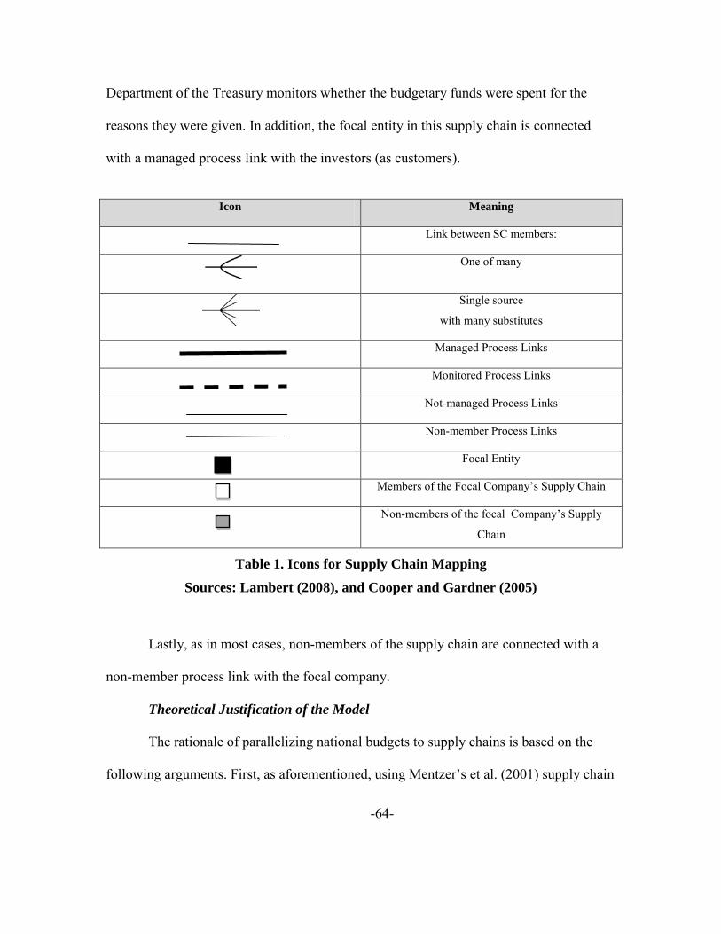
-64-
Department of the Treasury monitors whether the budgetary funds were spent for the
reasons they were given. In addition, the focal entity in this supply chain is connected
with a managed process link with the investors (as customers).
Lastly, as in most cases, non-members of the supply chain are connected with a
non-member process link with the focal company.
Theoretical Justification of the Model
The rationale of parallelizing national budgets to supply chains is based on the
following arguments. First, as aforementioned, using Mentzer’s et al. (2001) supply chain
Icon Meaning
Link between SC members:
One of many
Single source
with many substitutes
Managed Process Links
Monitored Process Links
Not-managed Process Links
Non-member Process Links
Focal Entity
Members of the Focal Company’s Supply Chain
Non-members of the focal Company’s Supply
Chain
Table 1. Icons for Supply Chain Mapping
Sources: Lambert (2008), and Cooper and Gardner (2005)

-65-
definition (“a set of three or more entities (organizations or individuals) directly involved
in the upstream and downstream flows of products, services, finances, and/or information
from a source to a customer”) a national budget is consistent with all the description and
the characteristics of a supply chain. As shown in the analysis conducted above, financial
and products/services flows exist in the conceptual model and there are numerous entities
involved in this upstream and downstream flow of information, financial funds and
product-services. The source is the entities that provide the funds to the government to
run the budget and the customers are the individuals and firms that are located in the
country’s territory as well as the investors that hold bonds. While the term “supplier
literally fits” in every case used in the conceptual model, the concept “customers” may
raise some questions: how can the citizens living in a country and the companies
stationed in its territory be characterized as the government’s “customers? The answer
lies in the definition of the word customer: A customer is “the recipient of
a good, service, product, or idea, obtained from a seller, vendor, or supplier for a
monetary or other valuable consideration”(Wikipedia, 2012). Within this framework, the
citizens, the companies and the investors, who have in their disposal government bonds,
can be considered as the government’s customers, as they receive the utility of the
(public) goods and services produced by the government, for a valuable consideration;
citizens and companies pay taxes, while investors buy bonds and receive profits
(interest).

-66-
Moreover, conceptually, relationship-based supply chain maps and budgets are
similar, in the sense that they both aim to allocate resources within a network of
organizations and their focus is the relationship between the entities they are comprised.
Practical Utility of the Model
Mapping - modeling a national budget as a supply chain can be beneficial in
various ways. First, based on Gardner and Cooper (2003), such a map helps to link the
whole supply chain (budget policy) with the fiscal policy. Moreover, a map may give a
signal for constraints in the whole system, i.e. as flows become apparent a supply chain
based map of a national budget reveals the actual government’s deficit and the magnitude
of debt, which can determine the limit of government’s borrowing capability. It can also
identify important entities for the supply chain’s operations, such as a group of taxpayers
that contributes substantially in the tax revenue gathered. Furthermore, it may act as a
basis for modifications or redesign of the government’s fiscal policy and it gives the “big
picture” of the national budget by transforming a mathematical equation into a
comprehensive figure, much friendlier to the reader. Additionally, it provides a common
understanding for the budget by visualizing the budget relationships and can act as a tool
for communication. Furthermore, such a map can be a means of training for policy
makers and can improve the budget’s management. Lastly, if the flows of goods/services
offered by the government to public (individuals and companies) are reported-mapped in
detail, the national budget supply chain map may be used as a basis for evaluating the
potential of outsourcing. Lastly, the potential of implementing supply chain techniques in

-67-
national budgets, with the intention of saving resources is a challenging approach of the
proposed conceptual model.

-68-
IV. Modeling and Exploring the Dynamics of the Budget Supply Chain as a System
Budget as a System
In this part of the thesis, research is focused on modeling the budget as a system
(Figure 13). Using as a basis the supply chain map introduced in the previous chapter and
taking into account the meaning and the definition of the term “system” already presented
in Chapter II, national budgets can be considered as systems with the following
components and characteristics:
Entities
The system’s entities consist of the tax payers (companies and individuals), the
government organization(s) responsible for forming and implementing the budget
(mainly the Ministry of Finance or the Department of the Treasury), the government
organizations that are recipients of budget funds and finally the investors, who obtain
government bonds.
Attributes
Each entity has various attributes. A good example of an entity’s attribute is the
taxable income of a taxpayer.
Activity
Imposing taxes, buying bonds in the credit markets and paying taxes are typical
activities of the government agency(ies) responsible for forming and implementing the
budget, the investors and the taxpayers, respectively.

-69-
Events
An event in the system may, for example, be a change in the interest rates
(exogenous event) or the application of a new tax (endogenous event).
State of the system
It is defined in any particular moment by a set of variables, such as the amount of
government deposits, number of taxpayers, amount of bonds sold, etc.
Flows
Considering the system’s components, as well as the map of the budget as a
supply chain, a model that presents the flows throughout the budget system is introduced,
using Forrester’s (1961) notation and symbols, (Table 5). In this model, the flows
between the focal entity (government) and the Tier 1 suppliers are financial (flows) and
represent the left part of the Government Budget Constraint (GBC), which is denoted by
the equation:
T + Δ𝐵𝑁𝑜𝑛−𝐺𝑜𝑣𝑡 +ΔM = 𝐺 + 𝑖𝐵𝑁𝑜𝑛−𝐺𝑜𝑣𝑡
Specifically, the financial flows from taxpayers to the government is the tax-
revenue (T), the flows between the investors in bonds and the government is the change
in the value of government bonds bought by non-government entities (ΔBnon-Govt) and the
flow from the central bank represents the change in the monetary base (ΔM). The first
two flows represent fiscal policy tools, while the last one stands for the monetary policy
applied. The special feature of the financial flow between the taxpayers and the

-70-
government is its compulsory character; taxpayers are obliged to pay the taxes
determined. They are either direct payments (income taxes, property taxes etc.) or
indirect, such as in the case of the indirect taxes, [Value Added Tax (V.A.T), fuel tax
etc.].
The flows between the entity in charge of applying the government’s policy
(Department of Treasury or Ministry of Finance) and the other government organizations
are internal and financial, in nature. Actually, they include the budget financial transfers
from the former to the later, in order for the government policies and programs to be
implemented. Subsequently, the flows from government agencies to individuals include
the supply of the public goods-services. The total cost of the public goods-services
offered from government organizations, plus the transfer payments compose the total
government spending (G).
Moreover, financial funds flow directly from the Department of Treasury or the
Ministry of Finance to investors that have government bonds in their disposal, in the form
of interest payments. In total, this flow represents the annual cost of government’s
borrowing (annual interest payments) and represents the value of iBnon-Govt in the
Government Budget Constraint.
Worth mentioning is that between the system’s entities there is a two-way flow of
information (downstream and upstream). For instance, there is an upstream flow of
information between the government agencies financed by the budget and the
organization responsible for the formation of it annually, in the preparation stage; the
former send their anticipated needs for the next fiscal year to the later. Another example

-71-
is the information flow that takes place between the government and the public in
general; the economic and budget policy is decided by the government, approved by the
appropriate legislative body (the Parliament or the Congress) and transferred to the public
by several means, such as by the Official Newspaper of the Government, by laws or even
by the media. Moreover, the government organizations responsible for the
implementation of the budget publish on a regular basis financial information and
extended budget data, concerning the GDP, the budget deficits, the public debt etc., so as
to communicate the situation of the public economics. Within this framework, usually
one year after the end of each fiscal year (i.e. 1-1-2012 for the fiscal year 2010), the
budget’s final balance sheet is given to the public, which contains detailed information
about the actual revenue gathered, the total amount of the outlays, the budget’s deficits or
surpluses etc. The comparison of the data on the balance sheet, with the information on
the budget for each year, determines how successful the implementation of what was
scheduled in the budget was. In addition, there is a continuous communication channel
among the organization responsible for the budget implementation and the agencies
financed by the budget, throughout the fiscal year, where useful information concerning
the budget and fiscal policy flows. Lastly, the information flow, among the
organization(s) responsible for the formation and execution of the budget and the tax
payers, literally constitutes the tax policy applied.
An interesting characteristic of the supply chain modeled is the direction of flows.
In typical supply chains there is a downstream flow of goods/services (except for returns)
and a reverse flow of financial funds. In this case, there is a financial flow of funds

-72-
downstream, with the exception of the flows between government and the last tier of
customers, where financial funds are also partially transformed to public goods and
services. Lastly, the exogenous variables that affect the budget are separately depicted in
the model.
Symbol Meaning
Flows of Goods and Services
Flows of Financial Funds
Flows of Information
Decision Function (Determine the Rate
of Flow)
Table 2. Symbols for Flow Diagrams
Source: Forrester (1961), “Industrial Dynamics”. P.82-83
Classification of the Budget Model - System
The model described above is descriptive according to Ragsdale’s (2008)
definition, given that the relationship between the variables is well defined by the GBC
equation, but there is uncertainty about the exact values of the independent variables (we
consider as independent variables the tax revenue T, the non-interest spending G and the
interest on the national debt iBNon-Govt, while the "dependent" variable is considered to be
the budget’s deficits, which is determined by the sum of the changes in the value of the
$ $

-73-
government bonds plus the change in the monetary base, given that the government will
either monetize the deficit or borrow to finance it). Moreover, following the classification
of models given by Forrester (1961), the budget model represented above is abstract, as it
consists of symbols, not physical objects and nonlinear, because any external effect on it,
is not purely additive (an analysis of the nonlinear character of the budget is conducted in
the next chapter). Moreover, the model is dynamic, in the sense that it deals with time-
varying interactions. In particular, former borrowing patterns affect the state of the
system, namely the interest that has to be paid annually is an outcome of the decisions
made in past fiscal years and vice versa what is decided concerning the fiscal and budget
policy in the present will affect future decision-making related to the budget. It can also
be characterized as unstable, because “an initial disturbance is amplified, leading to
growth or to oscillations whose amplitude increases”. Specifically, experience reveals
that the first deficits in the national budgets (initial disturbance for the balanced-budget
system) led to the amplification and oscillations of budget deficits and public debt (as
shown earlier, amplification is the U.S. public debt’s behavior, when measured in
nominal values and oscillation when it is measured as a percentage of the GDP). This
behavior is consistent with Forrester’s (1961) opinion, who stated that economic systems
are often unstable “wherein small disturbances grow in an unstable manner until
restrained by nonlinearities”. Such nonlinearities in the budget system are, in general, the
limited resources available after a point of deficits’ amplification, where investors deny
lending their money to countries with high deficits and public debt, or more frequently,
the decisions to cut deficits. In addition, the national budget system and model shows

-74-
transient behavior, as its “character” changes over time. Lastly, the rule for national
budgets is that they are nowadays open systems, as they are connected to exogenous
variables, which are created outside the model. Though, there are different levels of
openness in each case (i.e. usually countries which run budgets with deficits has more
“open” budget systems than those that run balanced budgets).

-75-
Figure 13. Modeling Budget as a System
T: Tax revenue
ΔBnon-Govt : Change in the value of
Government Bonds held by non-Govt
entities
ΔM: Change in the Monetary Base
G: Public Spending
ιBnon-Govt: Annual Interest for Govtm
Bonds

-76-
IV. The Dynamics of National Budgets as Systems
Dynamics of National Budgets: Theory and empirical evidence
National budgets, like supply chains, are complex and dynamic systems. Their
complexity doesn’t involve only the conventional perception about complexity, which is
mainly determined by the number of components that comprise a system (millions of
taxpayers and companies), but it is derived by the system’s dynamic complexity, too. In
this chapter, the major sources of budgets’ dynamic complexity are identified and it is
indicated where Keynesian Theory and Balanced-Budget Theory can fail, concerning the
deficits and public debt management.
Dynamics of the Budget System
Dynamics of a system are determined by the feedback processes, the stock and
flow structures, the time delays and the nonlinearities that exist inside it (Sherman, 2000).
Feedback Loops
Simply defined, a feedback loop exists when element A in a system affects
element B, which in turn affects element C, which at last affects element A (Toole and
Hufford, 2004). Generally, the meaning of feedback loops is described by the statements
that a system reacts to interventions, which also have unanticipated side-effects to the
system when applied (Sterman, 2000), and that any activity in a system affects at last the
element that initially performed the activity (Größler et al, 2008). According to Sterman
(2000) there are two kinds of feedback loops: The positive feedback loops that are self-
reinforcing and the negative loops that are self-correcting.

-77-
Representing the feedback structure of Systems with Causal Loop
Diagrams
Feedbacks in a system can be represented with Causal Loop Diagrams (CLD),
which belong to the word-and-arrow diagrams and are widely used in system dynamics
and systems thinking (Richardson, 1997). Sterman, (2000) devoted a whole chapter to the
concept of CLD, in which they (CLDs) are acknowledged as an important tool for
depicting the feedbacks in a system. Specifically, a causal diagram contains variables,
which are connected with arrows and which show a causal relationship. Positive
correlation between the independent and the dependent variable is denoted with (+) ,
while if the former affects the later negatively, it is denoted with a (-). In particular, a
positive link means that “if the cause increases the effect increases above of what it
would be otherwise have been and if the cause decreases, the effect decreases below what
it would otherwise have been” (Sterman, 2000). The opposite happens when two
variables are connected with a negative link: “If the cause increases, the effect decreases
below what it would otherwise have been, and if the cause decreases, the effect increases
above what it would otherwise have been” Sterman (2000). The important loops in a
CLD are highlighted in the diagram with what is known as a loop identifier, which shows
if the loop is negative or positive.
Figure 14 shows a typical example of a causal loop diagram. When the customer
base increases, all else equal, then the sales from word of mouth will be increased above
what it would have been, which in turn, will trigger a further increase of the customer
base. On the other hand, if the customer base increases customer loss rate increases, too,

-78-
and this leads to a tendency of restricting the customer base. In the first case, we have a
reinforcing (positive) feedback loop (denoted by R), while in the second one there is a
balancing (negative) feedback loop (denoted by B).
Figure 14. Causal Loop Diagram Notation
Source: Sterman, “Business Dynamics”, 2000
In the budget system as presented above, it is apparent that feedback loops are
present as taxpayers, companies and investors are the source of the inputs in the system,
as well as the recipients of the output; they share, at the same time, the role of supplier
and customer in the supply chain model. So, their behavior affects themselves because of
this feedback. For instance, if taxpayers do not pay their taxes, they will receive a lesser
“amount” of public goods and services or they will have to pay higher taxes in the future,
if the lower than expected tax revenue, is financed by borrowing (creation of deficits).
-
+ R B
+
+
Customer Base
Sales of Word of Mouth
Customer Loss Rate

-79-
Feedbacks in the Keynesian Model
As aforementioned the Keynesian Theory is based on the assumption that in times
of recession governments should run budgets with deficits, in order to stimulate the
economy. Such behavior will increase income, help the economy grow and finally reduce
the Debt-Income (GDP) ratio in the future. Approaching the Keynesian Theory from a
system view, the following Causal Loop Diagram (CLD) (Figure 15) was generated. In
this CLD there are two feedback loops. The main variable in the system is the budget
deficit. The right balancing feedback loop is a representation of the Keynesian Theory:
when deficits are generated, growth is created, too. That means that the income (GDP)
will be increased and so the tax revenue will also, which finally reduces deficits. Though,
there are two main prerequisites, in order Keynesian Theory to be accurate: The first is
that the deficits will be invested in activities that will generate growth and will increase
the GDP (the increase must be high enough to create revenue that will be adequate to
repay the borrowed amount of funds and the interest as well). The second is that a part of
the increase in the tax revenue, because of the amplification of the GDP, will be used to
repay the deficits created.
On the other hand, when deficits increase so does the public debt (left part of
Figure 15). This in turn, increases the annual interest that should be paid by budget funds
annually and there is a tendency for deficits to be increased (or surpluses to be reduced).
This is the reinforcing side of the CLD. The final outcome of the policy applied
concerning deficit depends on the magnitude of the two opposite tendencies.

-80-
Figure 15 is a justification of the intertemporal GBC, which states that the
Debt/GDP ratio can be reduced if the nominal value of debt increases, though, given that
the output growth (loop on the right) is greater than the real interest rate (loop on the left).
Figure 15. Feedback of the Keynesian Model
Feedbacks in the Balanced-Budget Model
In contrast to the Keynesian approach, the advocates of balanced budgets
underscore the need to eliminate or at least reduce deficits. Deficits are reduced either by
cutting spending or/and by increasing tax revenue, through a tax rates increase. In both
cases feedbacks are present.
Typically, in the case, of increasing tax rates, it is expected that the tax revenue
will be greater than before. This is not always true; according to the Laffer’s curve, when
the level of a tax (i.e. tax rate) exceeds a certain point (point T in Figure 16), the revenue
+ -
(+)
R B +
+ (-)
+
Deficit (Surplus)
Debt GDP
Annual Interest for bonds
Growth
Tax Revenue +

-81-
raised by the tax will be reduced. Point T represents the optimal tax rate that maximizes
tax revenue. Setting tax revenue at any other point than T will cause a reduction in tax
revenue.
Figure 16. The Laffer Curve
This is justified by the fact that real systems react to interventions, and entities’
actions trigger unanticipated side effects. In this case, taxpayers, after point T, reduce
their consumption of the taxable object, in the case of an indirect tax or they work less in
the case of an income tax (reaction and unanticipated side effect), which in turn offsets
the increase in receipts from increasing the tax rate. The outcome of this behavior is the
opposite of what was targeted (policy resistance). Instead of an increase, tax revenue
finally will be reduced. In other words the Laffer curve can be considered as a case of
feedback loop, which is described in the CLD of Figure 17. In particular, when T* (actual
tax rate) is less that T (higher point in the Laffer curve) tax revenue will be increased
(Case A). On the contrary, if T*>T (Case B), then a feedback loop is triggered, which
may lead budget and fiscal policy to a “death spiral”. Specifically, when T* surpasses T,
the side effects abovementioned are activated and consequently tax revenue declines.
Tax
Rev
enue
Tax Rate
T

-82-
With any other factor and variable unchanged, this leads to an increase of the budget
deficits (we assume that the deficits are covered by borrowing), which may cause a
decision of increasing tax rates further, that will, in turn, result in even greater deficits.
For example, in 2010 the Value Added Tax (VAT) was raised in Greece from 19%,
subsequently to 21% (15/3/2010-Law.3833/2010) and to 23% (1/7/2010-Law.
3845/2010). Although, both changes targeted to increase tax revenue raised by VAT, the
measures finally caused the reduction of VAT receipts; VAT revenue for 2010 reached
the mount of €15.52 billion while in 2012 it is estimated that the revenue raised by the
V.A.T will be €14.89 billion.
When it is tried to reduce deficits by cut spending , the outcome is uncertain, too.
There is a potential of policy resistance, as in the case of increasing tax rates. As shown
in the following CLD (Figure 18), when a decline in public spending is decided, two
opposite reactions are activated inside the budget system. The first one tends directly to
reduce the budget deficit, while the second tends to increase it, as cutting outlays tends to
reduce the income or/and the consumption and consequently the tax revenue. The final
outcome, namely whether deficits will be reduced, eliminated or a surplus will be created,
depends on the magnitude of these two opposite behaviors.

-83-
Figure 17. CLD when tax rates increase
Deficit (Surplus)
+ (-)
- (+)
+
+
-
Tax Revenue
+
Tax Rates
A & B
Side Effects
DELAY
DELAY
DELAY
Deficit (Surplus)
+
+ (-)
-
A. If T* < T, where T* is the actual tax
Tax Revenue
- (+)
+
+
Deficit (Surplus) Tax Rates
Tax Revenue
Tax Rates
B. If T* > T, where T* is the actual
Side Effects
DELAY
DELAY
DELAY

-84-
Figure 18. CLD when tax rates increase
Time Delays
Delays are “critical in creating dynamics … [they] give systems inertia, can create
oscillations, and are often responsible for trade-offs between the short- and long-run
effects of policies” (Sterman, 2000). Moreover, according to research studies, time delays
are commonly ignored, even when people know about their existence and their contents,
and lead to overshoot and instability (Sterman, 2000).
Time delays are another characteristic present in the national budget process.
Time is essential between deciding and implementing a change, and finally cause the
effects targeted; when a new tax or a change in the rate of an existing tax is decided, time
is needed for the proposal to become a law; thereafter time is needed in order for the
-
- (+)
-
Deficit (Surplus)
+
+ (-)
-
Tax Revenue
-
Cut Spending
Income
Consumption
DELAY
DELAY
DELAY
DELAY

-85-
receipts of the new tax to be gathered, too. Moreover, when financial funds are needed,
there is a minimum amount of time required, so as the whole process of borrowing and
receiving the money can be completed. Furthermore, bureaucracy in the budget system
creates delays. For instance, there is delay in the transfer of the budget funds from the
organization responsible for the budget to the government agencies which are financed
from it. A same type of delay, due to bureaucracy, occurs in the case of providing the
public goods-services. These are only some typical examples of time delays in the budget
system.
Problems arise when policy makers do not consider the presence of time delays,
conduct analysis concerning the effectiveness of the policies applied early and continue
to intervene into the system, as they think the policy implemented will not succeed its
goals. This leads to excess interventions, which jeopardize the system’s (budget) stability
and the success of the policies applied. Let’s take, for instance, the case of tax policy. If,
for whatever reason, it is decided to be changed, and time delays are not taken into
account, policy makers may intervene again into the system, causing sometimes
unanticipated behavior. In our previous example, if after the increase in the indirect tax
rate, policy makers do not allow enough time to find out the amount of revenue that will
finally be gathered by this change, they may increase even more the tax, so as to achieve
the receipts goal. This may lead taxpayers to reduce consumption of the taxable object at
a rate, that will finally reduce the revenue gathered by this indirect tax (exceed point T in
Laffer’s curve). In the present research study, delays were depicted in the budget model,
as well as in the CLDs.

-86-
Nonlinearities
Budgets are non-linear and cases of nonlinearities are apparent in the whole
system. For example, tax rates and tax revenue are not connected with a linear
relationship, as the principles of superposition [f (x + y) = f (x) + f (y)] or/and
homogeneity [f (kx) = kf (x)] are not satisfied. In particular, an increase of 10% in tax
rates does not essentially mean that tax revenue will be raised by 10%, because of the
side effects that the tax rate increase has to the budgetary elements (particularly to
taxpayers).
Stocks and Flows
National budgets, as shown in the supply chain model above, are typical systems
of financial, product and services, and information stocks and flows. Research showed
that “people’s intuitive understanding of stocks and flows is poor” (Sterman, 2000), and
this is why stocks and flows should be strongly considered in the budget preparation and
implementation stages.

-87-
V. Reengineering the Budget Process: Utilizing the Supply Chain Demand Management Process in Budgeting
Introduction
Based on the analysis conducted above, it is concluded that whichever philosophy
is adapted (the Keynesian model or the Balanced-Budget theory) it would be useful to
approach a budget as a supply chain system, and focus on its dynamics, in order to
approach the issues of budget deficits and public debt. At first, special attention should be
given to the feedbacks that are present in the system. Specifically, in the Keynesian case,
budget policy should be focused on the repayment of the deficits that financed the GDP’s
growth and on the income’s increase per se (as it is implied by the intertemporal budget
constraint too, the GDP’s increase should be high enough to create adequate tax revenue
that will be used to pay back the deficit caused). On the other hand, in the Balanced-
Budget approach, focus should be given to the causal effects of the actions taken to
control debt and reduce/eliminate deficits (increase in tax rates and/or cut in public
sending), that results in the opposite of the policy’s targets. Furthermore, in both cases
time delays, stocks and flows and nonlinearities, that exist in the system, should be
identified and considered when designing or/and implementing budget and fiscal policy.
The potential outcome of not considering the abovementioned, will be the creation of
dynamic complexity, which may be the cause of policy resistance (the interventions to
reduce/eliminate deficits and control public debt may be defeated by the system’s
response to the interventions itself). In particular, experience shows cases where when the
Keynesian model was followed, deficits financed growth, but deficits continued to

-88-
increase, even in “boom” economic periods. Likewise, there are cases where the effort to
balance the budget led to opposite of what was targeted, namely resulted in further
deficits and higher level of debt, too.
In the author’s perception, the solution to avoid or face the problems caused by
the dynamic character of the budget system is twofold. First, the whole budget process
should be reengineered on a basis that will reveal in real time or early enough the
feedbacks, the time delays, the nonlinearities, and the system’s stocks and flows, in order
to prevent the whole system from the unanticipated effects, which these phenomena cause
to the national budget. Second, the national budgets’ dynamics (feedbacks, time delays,
nonlinearities, stocks and flows) must be communicated to policy- and decision-makers,
students, even to individuals or/and generally to anyone interested in public economics,
so as national budgets to be approached as dynamics systems.
Reengineering the Budget Process: Utilizing Supply Chain Demand Management Process in Budgeting
Reengineering a process involves “the fundamental rethinking and radical
redesign of the process, to achieve dramatic improvements in critical, contemporary
measures of performance, such as cost, quality, service, and speed” (Hammer & Champy,
2003). Furthermore, demand management, as presented by Lambert (2008), is the process
that intends to balance the customer’s requirements with the supply chain capabilities. It
is not restricted to just forecasting, but it also includes the synchronization of supply and
demand, the increase of flexibility and the reduction of variability, and “can enable a

-89-
company to be more proactive to anticipated demand, and more reactive to unanticipated
demand”.
Taking into account these two definitions, it can be supported that a national
budget is a process of balancing outlays to revenue, by synchronizing supply and demand
for financial funds. In that sense, a national budget can be formed and implemented
according to the demand management supply chain process principles. Lambert (2008)
offers a framework of implementing the demand management process to supply chains,
which can be used as a basis for reengineering the budget process, too.
The demand management is segmented into two levels: the strategic and the
operational. Each of them consists of sub-processes. While the strategic sub-processes
define the structure of managing the process, the operational level consists of the
necessary day-to-day operations determined by the strategic sub-processes, which is
consistent with the reengineering concept (according to Hammer and Champy (2003)
reengineering first determines what to do and then how to do it). Both strategic and
operational sub-processes of the supply chain demand management process are shown in
Figure 18. Based on this structure, a framework to reengineer the budget process is
introduced in the following paragraphs.
The Budget Team
Initially, the national budget team should be formed and staffed with the necessary
personnel. Participants should not be limited only to members of the organization(s)
responsible for forming, implementing and reviewing the budget (Ministry of Finance or
The Department of the Treasury). Instead, the team should include members of all the
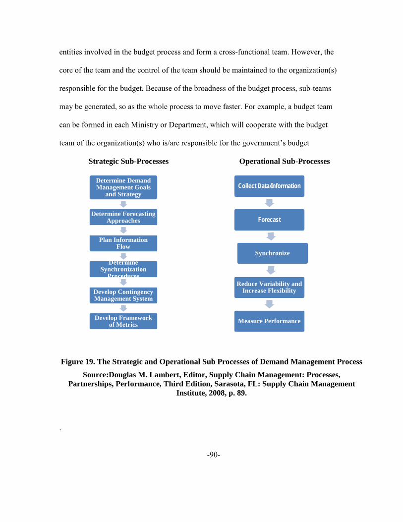
-90-
entities involved in the budget process and form a cross-functional team. However, the
core of the team and the control of the team should be maintained to the organization(s)
responsible for the budget. Because of the broadness of the budget process, sub-teams
may be generated, so as the whole process to move faster. For example, a budget team
can be formed in each Ministry or Department, which will cooperate with the budget
team of the organization(s) who is/are responsible for the government’s budget
Strategic Sub-Processes Operational Sub-Processes
Figure 19. The Strategic and Operational Sub Processes of Demand Management Process
Source:Douglas M. Lambert, Editor, Supply Chain Management: Processes, Partnerships, Performance, Third Edition, Sarasota, FL: Supply Chain Management
Institute, 2008, p. 89.
.
Determine Demand Management Goals
and Strategy
Determine Forecasting Approaches
Plan Information Flow
Determine Synchronization
Procedures
Develop Contingency Management System
Develop Framework of Metrics
Collect Data/Information
Forecast
Synchronize
Reduce Variability and Increase Flexibility
Measure Performance

-91-
The Strategic Budget Process
The strategic budget process consists of the same 6 sub-processes, as in the case
of the demand management process in the supply chain and targets to establish an
operational system that matches supply with demand. Figure 20 shows these processes, as
well as the budget stages, that each of them should be executed in. An brief analysis of
each sub-process is conducted below.
Figure 20. Strategic Sub-Processes and Stages of the Budget
Determine Demand Management Goals and
Strategy
Determine Forecasting Approaches
Plan Information Flow
Determine Synchronization Procedures
Develop Contingency Management System
Develop Framework of Metrics
Review Stage of the Budget
Implementation Stage of the Budget
Preparation Stage of the Budget
-92-
Determine Budget Goals and Strategy
In the first sub-process, the goals of the budget and the strategy that will lead to
the accomplishment of these targets, must be identified. A potential statement of
determining the budget goals and the strategy to achieve them is: “Reducing deficits by
increasing taxation”. Usually, neither budget goals nor strategy is in the budget team’s
authority boundaries. Rather, both are determined, usually, with the team’s cooperation
by the general economic policy applied.
Determine Forecasting Procedures
The second sub-process is related to forecasting. The budget team has to select the
appropriate methods of forecasting the flows throughout the budget’s supply chain.
Specifically, the team has to forecast, in the preparation stage, the level of tax revenue
which depends on the tax rates imposed, the potential amount of borrowing that will be
needed, the total government spending and the interest or/and principal, that has to be
paid back from previous loans.
It is logical that for each case a different forecasting approach should be applied.
Needs for spending are determined by a simple bilateral procedure between the
organization that prepares and implements the budget and the other major organizations
that are financed directly from it. Specifically, the former asks the later for their financial
needs for the next fiscal year in the preparation stage and proposes which part
(percentage) of the requests will be satisfied. The final decision of the amount that each
government organization will be financed with, belongs to the legislative body, which is
authorized to vote for and approve the budget. Adversely, tax revenue estimates are

-93-
harder to be precise, because the tax payers’ attitude to changes in tax policies is difficult
to be predicted. For example, as shown before, if the percentage of an indirect tax is
increased, it is not sure that the tax revenue will be greater than before; reduction in
consumption may be high enough to offset an increase in revenue. Lastly, forecasts about
borrowing financial funds depend on how successful the tax policy is.
Forecasts in the whole system should be as precise as possible. Poor flow
predictions, especially in the case of tax revenue, can affect negatively the
implementation of the budget; if revenue is finally less than anticipated, the gap has to be
filled by creating debt (borrowing) or by cutting expenditure or by monetization of
deficits, which may have undesired effects to the whole economic system. As forecasts
are based on data, the budget team should determine in this phase the sources, that will
provide the information needed for making the necessary estimations.
Plan Information Flow
The last step in the preparation stage for the budget team, is to plan the
information flow. In particular, the team must determine the means and other details of
transferring the data, as well as which part of the data will be communicated to whom.
For instance, although in earlier years the budget’s info were communicated through
mail, nowadays data transfer is conducted through IT applications, which saves time,
financial resources and, additionally, reduces bureaucracy.
Reverse information flow from the organizations financed by the Ministry of
Finance or the Department of the Treasury is another important aspect of this sub-
process. As financial funds flow from the later to the former, a plan for reverse

-94-
information flow should be established, in order to be audited, if the funds were used for
the reasons they were released for.
Determine Synchronization Procedures
The next two sub-processes are related to the implementation stage of the
budget. The first one involves the determination of the synchronization procedures that
need to be established, in order to match the forecasts for financial needs (government
spending and annual interest payments) to revenue and borrowing. At the strategic level,
that means to generate a plan of automated procedures, which will be applied at the
operational level and will align financial needs to funds’ supply. An important aspect of
this sub-process is the decisions that have to be made by the budget team, concerning the
allocation of resources. Specifically, when tax revenue is greater than projected and a
surplus is created, there must be a prediction of where the amount of the surplus will be
used for. For instance, it may be kept as inventory for future use or it may be used to buy
back additional bonds that mature in the near future, so as to reduce the debt. Another
possibility is to be used to increase funding in activities, which are already in progress.
Though and most importantly, in cases where financial flows to government’s
organization accountable to run the budget (tax revenue) is not adequate to finance the
already approved outlays, an automated procedure with generic guidelines should be
present, in order to allocate the insufficient recourses among the other government
organizations. Lack of synchronization procedures in this stage of the budget can affect
the government’s operations and consequently the economy and the society, too. As in

-95-
the case of a typical supply chain, software solutions, such as SAP can be applied so as to
facilitate the synchronization and pinpoint potential constraints in the whole system.
Develop Contingency Management System
Budgets and supply chains are complex. National budgets are dominated
by uncertainty, especially, about the tax revenue that is going to be collected during the
fiscal year, about the terms of loans (interest rates) which will prevail the moment that
there will be a need to borrow and finally, about the funds that will be needed to face
unpredicted events and situations (emergencies such as physical catastrophes i.e.
restoration of a road, damaged by a tornado). Within this framework, it is important for
the organization responsible for the implementation of the budget, to develop
“contingency plans to respond to significant internal and external events that disrupt the
balance of supply and demand” (Dobie et al., 2000). For instance, there must always
exist an amount of financial funds, which will be used only in emergencies and namely
operate as a “safety stock”. Generally speaking, there should be documented contingency
plans for every possible anticipated case, which may cause a disruption in the budget
supply chain. These plans must be rational and must include plans for immediate reaction
to every possible threat, that can affect negatively the flows among the entities of the
budget supply chain.
Develop Framework of Metrics
The last sub-process at this level consists of developing a framework of
metrics and concerns the last stage of the budget. It is important that there is a uniform
approach and a common understanding of these metrics throughout the members of the

-96-
supply chain (Lambert and Pohlen; 2001). A metric maybe the ratio of the actual outlays
to the outlays projected in the budget.
The Operational Budget Process
In this level, all the organizations involved in the budget process must apply what
was designed in the strategic level and they must make an effort to reduce variability in
their demand and increase flexibility in executing the budget. The operational budget
process contains five sub-processes, which are presented below.
Figure 21. The Operational Sub Processes of Demand Management Process
Collect Data/Information
Forecast
Synchronize
Reduce Variability and Increase
Flexibility
Measure Performance
Preparation Stage
Implementation Stage
Review Stage

-97-
Collect Data/Information
As mentioned above, at the strategic level, the budget team identifies the sources
of data on which the forecasts will be based on (Determine Forecasting Procedures sub-
process) and the channels through which the appropriate information will flow
throughout the supply chain (Plan Information Flow sub-process). The first step, at the
operational level, is to collect the necessary data for synchronizing the budget’s supply
and demand. Collection of data takes place initially in the preparation stage of the budget
process; the budget planner asks from the government’s organizations to state their needs
for the upcoming fiscal year and receives their applications for financing. So, in this stage
the government entities make their forecasts for necessary financing. Collection of data,
in the budget process, does not stop in the preparation stage. On the contrary, in the stage
of the implementation, the organization responsible for the budget does collect data on a
regular basis for the spending of the funds granted to the other government organizations
and for the tax revenue gathered, and publishes, as stated before, statements with this data
throughout the fiscal year. Moreover, in the audit stage, the organization responsible for
the budget collects data that is related to the budget, so as to conduct the appropriate
checking.
Forecast
After obtaining and taking into account the data from the government
organizations for their financial needs, the budget team conducts its own forecast for
aggregate demand for financial funds. Worth mentioning is that in this sub-process, the
sum of the requested funds is not necessarily equal to the aggregate demand forecasted by

-98-
the budget planner, because it is likely that some of the demands will not be satisfied, due
to insufficient resources.
Synchronize
As the forecast of financial needs has been made by the budget team, the next step
is to synchronize supply and demand. That is to collect the taxes and borrow, if needed,
any additional funds, and transfer them to the government agencies according to the
budget’s guidelines.
Reduce Variability and Increase Flexibility
In this sub-process the budget team has a twofold goal. First, variability has to be
reduced in the whole system. Focus should be given in the variability of the tax revenue.
As it determines the success of the budget policy on a large scale, appropriate measures
should be taken, so as to reduce cases of deviations, between the anticipated tax revenue
and the actual tax receipts. Though, as variability is unavoidable, flexibility should be
built in the budget system, too. The budget team should be flexible enough to face any
disturbance in the whole system. In the previous example, there should be appropriate
mechanisms that will cover the gap between the expected and the actual tax revenue, such
as an amount that will be kept to the treasury as a “safety stock”.
Measure Performance
In the last sub-process, the budget team must measure the performance of each
year’s budget, according to the metrics developed in the strategic level. For instance, a
measure of performance maybe the ratio of the actual tax receipts to the anticipated tax
revenue.

-99-
The role of Information Technology to Reengineering Budget - Conclusions
The whole reengineering process as described above will help policymakers and
the budget team to identify early enough and react to the feedbacks, triggered by the
interventions to the system. Moreover, a budget process based on Lambert’s principles
will reveal the time delays, stocks and flows and nonlinearities, when they appear in the
system. For instance, in cases where revenue falls short of what was projected and/or
where government organizations delay in the implementation of their programs, will be
signaled in the system, so as corrective actions can be taken. It is apparent that a well-
structured communication channel is a prerequisite for these signals to show up in the
system, when a disturbance occurs. In general, Information Technology (IT) is a key
player to reengineer the budget process. Transfer and monitoring of real-time data is a
requirement for success. In that sense, IT is the main enabler of achieving a reengineered
budget process, but it is not adequate per se.

-100-
VI. The Budget Management Flight Simulator
Introduction
Considering a national budgets’ dynamic complexity described above, which
results in phenomena of policy resistance, we now proceed to the second step of a typical
system dynamics project, which is “Simulation/Experiments”, by introducing a proposal
for a Management Flight Simulator (MFS). Its mission will be to develop a learning tool
for policy-makers, students and any others interested in public economics, which will
reveal the dynamics of the national budget system, as the Beer Game does in the case of
the supply chain. Its utility and necessity derives from the fact that there are a lot of
misperceptions and misunderstanding about fiscal and budgetary policy, deficits and
debt. Particularly, there are people who think that drastic reductions in outlays or/and
radical increases in tax rates will solve the problem of debt, while others believe that just
stimulating the economy with further deficits will increase income and the public debt
will be controlled. Both approaches ignore the feedbacks, death spirals, delays and
nonlinearities existent in the budget system. In other words, like in the case of the supply
chain with the Beer Game, a similar tool should be developed, that will expose simply
and comprehensively the complexity of the budget system.
It should be mentioned that the establishment of a MFS concerning the national
budget and the fiscal policy is a novel idea, but the development of the simulation
software goes far beyond the scope of this research study. Though, it is intended to be the
next assignment of the author of the present thesis.
-101-
General Concept - Rules
The purpose of the MFS is to show players that budgets are dynamic systems,
where feedbacks, delays, nonlinearities, and stocks and flows produce dynamic
complexity, which in turn is a main cause of policy resistance. Within this framework, the
player in the simulation will be given the role of the decision-maker, concerning the
budget and the fiscal policy, and a certain target of public debt and/or budget
deficit/surplus will be assigned to be achieved. Thereafter, certain scenarios of fiscal
policy and budgetary issues will be produced by the simulator and the player will have to
make decisions to face these situations, from a predetermined menu of choices. Each
choice will have an impact on the budget’s deficit and on public debt, and the player’s
performance will be evaluated due to the final outcome that his decisions will have on the
deficits-surplus-debt. The main purpose of the MFS will not be to create a game of
competition, although good results are the players’ target. Rather, the main objective will
be to familiarize players with budget’s complexity, by presenting examples in which
budgets behave as systems that typically resist changes. Within this framework, “real”
policy resistance cases should be included and emphasized in the scenarios presented.
Considering the abovementioned, an example is presented below that shows a potential
scenario-question of the MFS:
Scenario-Question: Reports for the outlays needs have been received. After a
close exanimation, it is found that $X extra billion of outlays will be needed for the
healthcare bill for the next fiscal year. You obtain these extra funds by:

-102-
A. Issuing Bonds and Borrowing $X billion
B. Raise the Sales Tax by 2%
In case the player chooses answer A, there will be an increase of debt by $X
billion. On the contrary, if he chooses answer B, although it will be expected the revenue
to be increased the impact on the debt will be greater that $X billion, for instance $Y>X
billion. Of course, it will be explained to the player that this is not an arbitrary result of
the simulator, but the outcome of his decision: By raising sales tax by 2%, consumption
declined, because prices increased and this caused the revenue’s reduction. This paradigm
that lies in the Laffer’s curve, will teach players that interventions in the budget system
(i.e. a raise in the tax rates) may trigger the opposite behavior and results than those
anticipated, because they cause side effects (reduction in consumption) that may even
outpace the intervention’s outcomes. It would be ideal to connect these scenarios-
questions with real data (find a real case where, when sales tax was raised, actual tax
revenue was reduced) and present them to players, in order to emphasize the budget’s
dynamics and give credibility to the MFS.
Technically, the first version of the MFS will be a one player simulator; later
versions may include more players. In addition, the simulation software that will be
chosen for the MFS, should be relevant to the needs of the study and “friendly” to the
user. Moreover, after being created and tested, the Budget MFS should be forwarded for
use to anyone interested to enhance his understanding in public economics. Thereafter, it
is proposed to gather data and analyze the decision-makers’ behavior, like Sterman

-103-
(1989) did in the case of the supply chain with the Beer Game. It would be interesting,
novel and useful to investigate the potential of patterns in human behavior that has to do
with budgetary and fiscal policy decisions.

-104-
VII. Conclusions and Recommendations
The novelty of this research study lies in the fact that the national budget is
modeled as a system for the first time in the literature. An extensive analysis showed that
no other study has linked and/or applied, until now, the systems theory to the fiscal –
budgetary policy. Specifically, in this thesis, it is identified that the national budget is a
complex and dynamic system. Its dynamics consists of feedbacks, time delays, stocks and
flows, and nonlinearities, which cause dynamic complexity, jeopardize the achievement
of the budgetary goals and can be the source of policy resistance cases.
Within this framework, policy-makers, whether advocates of the Keynesian
Theory or loyal to the Balance Budget approach, should consider that budgets are
systems, consisting of a plethora of entities which interact within the system’s
boundaries. Any budgetary decision triggers various side effects, in addition to what is
intended and targeted, which should be considered in advance or, if it is not possible to be
predicted, as soon as they appear in the system. Special attention should be given to
exogenous variables that affect the system and tend to influence the budget’s and its
entities state, too.
Identifying dynamic complexity is not a simple task. Rather, it is a challenging
issue. However, reengineering the budget process on the basis of the supply chain
demand management process, can result in identifying the budget’s dynamics early
enough to take action and avoid unwanted phenomena and results. Furthermore, as in the
case of the supply chain with the Beer Distribution Game, a Management Flight
Simulator should be developed, in order to act as a learning tool about the budget’s

-105-
dynamics and reveal the complexity of the budget as a system. In other words, its primary
purpose should be to emphasize the national budgets’ complex and dynamic character.
Another novelty of this research study is that national budgets were mapped as a
special case of a supply chain and modeled as a supply chain system. Of course, budgets
can be modeled as a different kind of system, too. Nevertheless, the supply chain
approach includes the characteristics needed to give a comprehensive and easily
understandable picture of the whole system.
Recommendations for Further Research
As aforementioned the novelty of the present thesis lies in the fact that the
national budget is considered to be and it is modeled as a system, specifically a supply
chain system. As such, this research study can be considered as the first step in a new
field of thinking, where budgets are modeled and analyzed as systems and/or supply
chains. In particular, this project contains the theoretical background of mapping and
modeling the national budget as a supply chain and as a system, respectively.
Within this framework, reengineering the budget process on the basis of the
supply chain demand management process, can result in identifying the budget’s
dynamics early enough to take action and avoid unwanted phenomena and results.
Furthermore, as in the case of the supply chain with the Beer Distribution Game, a
Management Flight Simulator should be developed, in order to act as a learning tool
about the budget’s dynamics and reveal the complexity of the budget as a system.
Specifically, areas of potential future research may enclose a case study where a
country’s budget will be modeled as a supply chain system or just as a system.

-106-
Furthermore, follow-up research may include the identification of cases where the
budget’s dynamics caused the opposite results of what was targeted by the policies
implemented (case studies of policy resistance caused by the budget dynamics). In
general, this study introduced the idea that budgets are systems and further research may
focus on additional issues concerning the implementation of system’s theory to
budgeting.
Furthermore, in this study, it is introduced a conceptual basis for reengineering
the national budget procedure, according to the postulates of the demand management
process of a supply chain. Future researchers and policy makers may consider this
framework when proposing or applying changes to their countries’ budgeting process.
Finally, the present thesis makes a proposal to develop a Management Flight
Simulator for national budgeting. Future research must, in the author’s opinion, include
the establishment of a Management Flight Simulator, concerning the national budget’s
dynamics. It is not only that the MFS will be useful to policy makers, students or
academics; if it is, as simple and successful in accomplishing its purposes as the Beer
Distribution Game, in the case of the supply chain, it will make everyone understand
what a budget is: a system, whose dynamics (feedbacks, nonlinearities, stocks and flows,
and time delays) makes its management much more complex than it appears to be today.

-107-
Appendix A: OECD - Government deficit: Net lending/net borrowing as a percentage of GDP, surplus (+), deficit (-)
2006 2007 2008 2009 2010 2011 2012 2013 Australia 2.3 1.8 -0.8 -4.5 -4.7 -3.9 -2.2 0.4 Austria -1.7 -1.0 -1.0 -4.2 -4.5 -2.6 -2.9 -2.3 Belgium 0.3 -0.1 -1.0 -5.7 -3.9 -3.9 -2.8 -2.2 Canada 1.6 1.4 -0.4 -4.9 -5.6 -4.5 -3.5 -2.4
Czech Republic -2.4 -0.7 -2.2 -5.8 -4.8 -3.1 -2.5 -2.2
Denmark 5.0 4.8 3.3 -2.7 -2.7 -1.9 -3.9 -2.0 Estonia 2.5 2.4 -2.9 -2.0 0.3 1.0 -2.0 -0.3 Finland 4.0 5.3 4.2 -2.7 -2.9 -0.9 -0.7 -0.0 France -2.4 -2.7 -3.3 -7.6 -7.1 -5.2 -4.5 -3.0 Germany -1.7 0.2 -0.1 -3.2 -4.3 -1.0 -0.9 -0.6
Greece -6.0 -6.8 -9.9 -15.6
-10.5 -9.2 -7.4 -4.9
Hungary -9.4 -5.1 -3.7 -4.5 -4.3 4.2 -3.0 -2.9
Iceland 6.3 5.4 -13.5
-10.0
-10.1 -4.4 -2.6 -1.4
Ireland 2.9 0.1 -7.3 -14.0
-31.2
-13.0 -8.4 -7.6
Israel (1) -2.5 -1.5 -3.8 -6.4 -5.0 -4.4 -4.3 -4.2 Italy -3.4 -1.6 -2.7 -5.4 -4.5 -3.8 -1.7 -0.6 Japan -1.3 -2.1 -1.9 -8.8 -8.4 -9.5 -9.9 -10.1 Korea 3.9 4.7 3.0 -1.1 1.3 1.8 2.3 2.8 Luxembourg 1.4 3.7 3.0 -0.8 -0.9 -0.6 -1.4 -1.1 Netherlands 0.5 0.2 0.5 -5.5 -5.0 -4.6 -4.3 -3.0
New Zealand 5.3 4.5 0.4 -2.6 -4.2 -8.2 -4.4 -2.9
Norway 18.3 17.3 18.8 10.6 11.2 13.6 15.1 16.3 Poland -3.6 -1.9 -3.7 -7.4 -7.9 -5.1 -2.9 -2.2
Portugal -4.6 -3.2 -3.7 -10.2 -9.8 -4.2 -4.6 -3.5
Slovak Republic -3.2 -1.8 -2.1 -8.0 -7.7 -4.8 -4.6 -2.9
Slovenia -1.4 -0.0 -1.9 -6.1 -6.0 -6.4 -3.9 -3.0
Spain 2.4 1.9 -4.5 -11.2 -9.3 -8.5 -5.4 -3.3
Sweden 2.2 3.6 2.2 -1.0 -0.1 0.1 -0.3 0.3 Switzerland 0.8 1.7 2.3 1.0 0.6 0.8 0.6 0.6

-108-
United Kingdom -2.7 -2.8 -5.0 -
11.0 -
10.3 -8.4 -7.7 -6.6
United States -2.2 -2.9 -6.6 -
11.6 -
10.7 -9.7 -8.3 -6.5
Euro area (15 countries)
-1.4 -0.7 -2.1 -6.4 -6.2 -4.1 -3.0 -2.0
OECD-Total -1.2 -1.3 -3.4 -8.1 -7.5 -6.3 -5.3 -4.2 Last updated: 7 June 2012
1.
The statistical data for Israel are supplied by and under the responsibility of the relevant Israeli authorities. The use of such data by the OECD is without prejudice to the status of the Golan Heights. East Jerusalem and Israeli settlements in the West Bank under the terms of international law.
Source: OECD Economic Outlook No. 91. OECD Economic Outlook: Statistics and Projections (database)

-109-
Appendix B: General Government Gross Financial Liabilities as a percentage of GDP OECD Economic Outlook No. 91, OECD Economic Outlook: Statistics and Projections (database)
1994 1995 1996 1997 1998 1999 2000 2001 2002 2003 2004 2005 2006 2007 2008 2009 2010 2011 2012 2013
Australia 40.3 42.0 39.2 37.5 32.4 | 28 25.0 22.1 20.1 18.6 16.8 16.3 15.6 14.5 13.8 19.4 23.5 26.6 28.7 27.8 Austria 65.3 69.5 70.3 66.2 67.8 70.8 70.5 71.6 72.8 71.1 70.9 70.6 66.4 63.4 68.7 74.4 78.1 79.7 83.0 84.4 Belgium1 137.7 135.3 133.2 127.8 123.1 119.5 113.6 111.9 108.3 103.3 98.3 95.8 91.6 87.9 92.9 99.9 100.0 102.3 103.1 102.0 Canada 98.0 101.6 101.7 96.3 95.2 91.7 82.4 82.9 80.8 76.8 72.8 71.8 70.4 66.7 71.2 82.4 84.0 83.8 84.5 81.4 Czech Republic .. .. .. .. .. .. .. .. 31.5 33.2 33.2 32.8 32.5 31.0 34.4 41.0 45.5 48.3 50.7 52.6 Denmark 85.8 81.7 79.1 74.8 72.4 67.1 60.4 58.4 58.2 56.6 54.0 45.9 41.2 34.3 41.4 51.2 54.8 61.8 63.0 64.8 Estonia .. 13.3 12.3 11.3 10.0 10.9 9.4 8.9 10.2 10.8 8.5 8.2 8.0 7.3 8.5 12.7 12.5 10.0 12.7 12.8 Finland 60.7 65.3 66.2 64.7 61.2 54.9 52.4 49.9 49.5 51.4 51.5 48.4 45.6 41.4 40.4 51.8 57.6 57.2 59.1 61.8 France 60.1 62.6 66.4 68.9 70.4 66.9 65.7 64.3 67.5 71.7 74.1 76.0 71.2 73.0 79.3 91.2 95.8 100.1 105.5 107.3
Germany2 46.5 55.7 58.8 60.4 62.3 61.8 60.8 60.1 62.5 65.9 69.3 71.9 69.8 65.6 69.8 77.4 86.8 87.2 88.5 87.8 Greece .. 102.0 104.1 100.9 98.6 102.4 116.4 119.2 118.6 113.3 115.8 113.4 117.0 115.4 118.7 134.0 149.6 170.0 168.0 173.1 Hungary 91.9 88.5 76.8 67.0 65.2 67.5 62.1 60.0 60.7 61.7 65.5 68.7 71.9 72.9 77.0 86.2 86.4 84.7 84.8 84.1 Iceland .. .. .. .. 77.3 73.6 72.9 75.0 72.0 71.0 64.4 52.6 57.4 53.3 102.1 120.0 125.2 128.3 126.7 124.7 Ireland .. .. .. .. 62.6 51.7 39.7 36.8 35.8 34.5 33.1 32.9 29.0 28.6 49.5 71.1 98.4 114.1 121.6 126.9 Israel .. .. .. .. 101.0 94.8 84.3 89.0 96.7 99.3 97.7 93.7 84.7 78.1 77.1 79.5 76.1 74.2 73.9 73.2 Italy 120.3 121.9 128.1 129.6 131.8 125.7 120.8 120.1 118.8 116.3 116.8 119.4 116.7 112.1 114.6 127.7 126.5 119.7 122.7 122.1 Japan3 80.2 87.8 95.4 102.0 115.0 128.9 137.5 144.6 153.4 158.2 166.2 169.5 166.7 162.4 171.2 188.8 192.7 205.5 214.1 222.6 Korea4 .. .. .. .. .. .. .. .. 19.2 19.7 23.3 25.5 28.5 28.7 30.4 33.5 34.6 34.7 34.5 33.9 Luxembourg .. .. .. .. 16.2 14.8 13.4 13.5 12.2 13.1 14.0 12.1 11.5 11.3 18.3 18.0 24.7 23.9 26.0 28.7 Netherlands 86.6 89.5 88.0 82.1 80.7 71.6 63.8 59.4 60.2 61.3 61.9 60.7 54.5 51.5 64.8 67.5 70.6 75.2 81.0 83.6 New Zealand 56.8 50.7 44.3 41.7 41.6 39.0 36.9 34.9 33.0 30.9 28.2 26.9 26.6 25.7 28.9 34.5 37.4 44.3 48.4 50.5 Norway 34.6 37.9 33.6 29.7 28.0 29.1 32.7 31.8 39.0 48.4 50.9 47.8 59.0 56.8 54.3 48.9 49.6 34.0 28.1 20.2 Poland .. 51.6 51.5 48.4 44.0 46.8 45.4 43.7 55.0 55.3 54.8 54.8 55.2 51.8 54.5 58.4 62.3 63.3 62.9 62.3 Portugal .. 66.7 66.5 65.2 63.1 60.4 60.1 61.5 64.8 66.5 69.1 72.6 77.3 75.4 80.7 92.9 103.2 117.6 124.3 130.1 Slovak Republic .. 38.2 37.6 39.0 41.2 53.5 57.6 57.1 50.2 48.2 47.6 39.2 34.1 32.9 32.0 40.4 47.1 46.8 52.1 54.2 Slovenia .. .. .. .. .. .. .. 33.6 34.7 34.1 34.9 34.0 33.8 30.7 30.4 44.3 48.4 56.4 60.3 63.2 Spain 64.3 69.3 76.0 75.0 75.4 69.4 66.5 61.9 60.3 55.3 53.3 50.7 46.2 42.3 47.7 62.9 67.1 75.3 87.9 90.9 Sweden 82.5 81.1 84.4 83.0 82.0 73.2 64.3 62.7 60.2 59.3 60.0 60.8 53.9 49.3 49.6 51.8 48.9 48.7 48.0 46.0 Switzerland 45.5 47.7 50.1 52.1 54.8 51.9 52.4 51.2 57.2 57.0 57.9 56.4 50.2 46.8 43.6 42.5 41.7 41.0 40.8 39.4 United Kingdom 46.8 51.6 51.2 52.0 52.5 47.4 45.2 40.4 40.8 41.5 43.8 46.4 46.0 47.2 57.4 72.4 81.9 97.9 104.2 108.2 United States 71.1 70.7 69.9 67.4 64.2 60.5 54.5 54.4 56.8 60.2 68.0 67.6 66.4 67.0 75.9 89.7 98.3 102.7 108.6 111.2

-110-
Euro area 71.1 | 75.5 80.0 81.0 81.6 78.2 75.9 74.4 75.3 76.0 77.3 78.1 74.7 71.8 77.0 87.8 93.1 95.1 99.1 99.9 Total OECD 70.0 | 72.6 74.2 73.9 74.5 72.9 70.2 69.9 71.9 73.7 77.8 78.1 76.0 74.5 81.0 92.5 98.7 103.0 107.6 109.3
Note: Gross debt data are not always comparable across countries due to different definitions or treatment of debt components. Maastricht debt for European Union countries is shown in Annex Table 61. For more details. see OECD Economic Outlook Sources and Methods (http://www.oecd.org/eco/sources-and-methods).
For euro area countries with unsustainable fiscal positions that have asked for assistance from the European Union and the IMF (Greece. Ireland and Portugal) the change in 2010 and 2011 in government financial liabilities has been approximated by the change in government liabilities recorded for the Maastricht definition of general government debt (see Box 1.2 on policy and other assumptions in Chapter 1).
1. Includes the debt of the Belgium National Railways Company (SNCB) from 2005 onwards. 2. Includes the debt of the Inherited Debt Fund from 1995 onwards.
3. Includes the debt of the Japan Railway Settlement Corporation and the National Forest Special Account from 1998 onwards. 4. Data are on a non-consolidated basis
(SNA93). Source: OECD Economic Outlook 91 database.

-111-
Bibliography
Adam Smith. (1776). The wealth of nations, book V, chapter III
ALESINA, A. (1990). A positive theory of fiscal Deficits and Government Debt. The
Review of Economic Studies, 57(3), 403-414.
Aliabadi, S., Alireza, D., & Abdyldaeva, A. (2011). Budget deficit, national debt, and
government spending: Is now the right time to cut deficit and reduce national debt?
Journal of Accounting, Business & Management, 18(2), 74-83.
APOSTOLIDES, A. D. (1999). A historical perspective on the size of deficits and debts
in OECD countries. Budget Deficits and Debt: A Global Perspective, , 27.
Bakken, B., Gould, J., & Kim, D. (1992). Experimentation in learning organizations: A
management flight simulator approach. European Journal of Operational Research,
59(1), 167-182.
Banks, J., Carson, J. S., Nelson, B. L., & Nicol, D. M. (2010). Discrete-event system
simulation.
Barro, R. J. (1974). Are government bonds net wealth? The Journal of Political
Economy, 82(6), 1095-1117.
-112-
Barth, J. R., & Wells, J. M. (1999). Budget deficits and economic activity. Budget
Deficits and Debt: A Global Respective, Ed.Shojai, S.Westport, Connecticut:
Praeger,
Barth, J. R., Iden, G. R., & Russek, F. S. (1986). The economic consequences of federal
deficits: An examination of the net wealth and instability issues. Southern Economic
Journal, 53(1), 27. Retrieved from
http://search.ebscohost.com/login.aspx?direct=true&db=buh&AN=4631305&site=e
host-live
Black, J., Hashimzade, N., & Myles, G. D. (2009). A dictionary of economics Oxford
University Press, USA.
Bowles, E. (Mar 01, 2012). The danger of doing nothing. Harvard Business Review,
Burkhead, J. (1956). Government budgeting Wiley.
Caiden, N. (1998). Public service professionalism for performance measurement and
evaluation. Public Budgeting & Finance, 18(2), 35-52.
Congressional budget office. Retrieved May 20, 2012, from
http://www.cbo.gov/publication/43024
Cooper, M., & Gardner, J. (2005). Map your supply chain. CSCMP Explores, 2(Winter)

-113-
Croom, S., Romano, P., & Giannakis, M. (2000). Supply chain management: An
analytical framework for critical literature review. European Journal of Purchasing
& Supply Management, 6(1), 67-83.
Dornbusch, R., & Fischer, S. R. startz,(1998), macroeconomics.
Dornbusch, R., & Fischer, S. (Eds.). (1990). Macroeconomics (5th ed.) McGraw - Hill
Publishing Company.
Downes, J., & Goodman, J. (2006). Baron’s financial guide: Dictionary of finance and
investment terms.
Eisner, R., & Pieper, P. J. (1984). A new view of the federal debt and budget deficits. The
American Economic Review, 74(1), 11-29.
Elmendorf, D. W., & Gregory Mankiw, N. (1999). Government debt. Handbook of
Macroeconomics, 1, 1615-1669.
European Union. European financial stability facility (EFSF). Retrieved May 12, 2012,
from http://www.efsf.europa.eu/about/index.htm
Treaty on Stability, Coordination and Governance in the Economic and Monetary Union,
(Signed on 2 March 2012 by the EU Member Countries with the exception of the
United Kingdom and the Czech Republic, Not Published yet in the Official Journal
(OJ) of the European Union).

-114-
European Union, E. (7 June 2010). Spring 2010 orientation debate on budgetary
policies:Orientations for fiscal policies in euro area member states. Luxembourg:
Eurogroup.
Financial Times Lexicon. Austrian economics. Retrieved August 10, 2012, from
http://lexicon.ft.com/Term?term=Austrian-economics
Forrester, J. W. (1994). System dynamics, systems thinking, and soft OR. System
Dynamics Review, 10(2‐3), 245-256.
Forrester, J. W., & Massachusetts Institute of Technology. (1961). Industrial dynamics
MIT press Cambridge, MA.
Friedman, B. M. (1988). Day of reckoning: The consequences of american economic
policy under reagan and after Random House New York.
Galbraith, J. K. (2010). In defense of deficits. The Nation, , 22-24.
Gale, W., & Orszag, P. R. (2003). Economic effects of sustained budget deficits.
Ganeshan, R., & Harrison, T. P. (1995). An introduction to supply chain management.
Penn State University, the United States,
Ganeshan, R., & Harrison, T. P. (1995). An introduction to supply chain management.
Penn State University, the United States,

-115-
Gardner, J. T., & Cooper, M. C. (2003). Strategic supply chain mapping approaches.
Journal of Business Logistics, 24(2), 37-64.
Gregory, T., Hayek, F., Plant, A., & Robbins, L. (1932). Spending and saving: Public
works from rates. Times of London, 19, 10.
Größler, A., Thun, J. H., & Milling, P. M. (2008). System dynamics as a structural theory
in operations management. Production and Operations Management, 17(3), 373-
384.
Gupta, S., & Dutta, K. (2011). Modeling of financial supply chain. European Journal of
Operational Research, 211(1), 47-56.
Hackbart, M., & Ramsey, J. R. (2002). The theory of the public sector budget: An
economic perspective. Budget Theory in the Public Sector, , 172.
Hammer, M., & Champy, J. (2003). Reengineering the corporation: A manifesto for
business revolution HarperBusiness.
Hou, Y., & Smith, D. L. (2006). A framework for understanding state balanced budget
requirement systems: Reexamining distinctive features and an operational definition.
Public Budgeting & Finance, 26(3), 22-45.
http://www.shadowstats.com/
Hugos, M. H. (2003). Essentials of supply chain management Wiley.

-116-
International Monetary Fund. About the IMF. Retrieved May 15, 2012, from
http://www.imf.org/external/about.htm
International Monetary Fund. (2006). Glossary of selected financial terms. Retrieved
April 18, 2012, from http://www.imf.org/external/np/exr/glossary/index.asp
Jacobs, F. R. (2000). Playing the beer distribution game over the internet. Production and
Operations Management, 9(1), 31-39.
Kelton, S. (2011). Limitations of the government budget constraint: Users vs. issuers of
the currency. Panoeconomicus, 58(1), 57-66.
Keynes, J. M. (1936). The general theory of interest, employment and money.
Kouvelis, P., Chambers, C., & Wang, H. (2006). Supply chain management research and
production and operations management: Review, trends, and opportunities.
Production and Operations Management, 15(3), 449-469.
Lambert, D. M. (2008). Supply chain management: Processes, partnerships, performance
Supply Chain Management Inst.
Lambert, D. M., Cooper, M. C., & Pagh, J. D. (1998). Supply chain management:
Implementation issues and research opportunities. International Journal of Logistics
Management, the, 9(2), 1-20.

-117-
Lambert, D. M., Stock, J. R., & Ellram, L. M. (1998). Fundamentals of logistics
management Irwin/McGraw-Hill Chicago, IL.
Law, A. M., & Kelton, W. D. Simulation modeling and analysis
Liddell, H. G., & Scott, R. (1900). An intermediate greek-english lexicon Clarendon
Press.
Macgregor, D., Pigou, A., Keynes, J., Layton, W., Salter, A., & Stamp, J. (1932). Private
spending: Money for productive investment. Times of London, 17, 13.
Maier, F., & Strohhecker, J. (1996). Do management flight simulators really enhance
decision effectiveness? The 14th International Refereed Conference of System
Dynamics Society, Massachussetts, USA.
Mentzer, J. T., DeWitt, W., Keebler, J. S., Min, S., Nix, N. W., Smith, C. D., et al.
(2001). Defining supply chain management. Journal of Business Logistics, 22(2), 1-
25.
Michael, H. (2003). Essentials of supply chain management.
Milling, P. A management simulator to support group decision making in a corporate
gaming environment.
Musell, R. M. (2009). Understanding government budgets: A practical guide Taylor &
Francis.

-118-
O'Driscoll Jr, G. P. (2012). Keynes vs. hayek: The great debate continues. The Tea,
OECD. Public finance and fiscal policy. Retrieved May 15, 2012, from
www.oecd.org/eco/public_finance
OECD. (2011).
OECD economic outlook. OECD Economic Outlook, 2011(2)
OECD. (2012). OECD factbook 2011-2012: Economic, environmental and social
statistics OECD Publishing.
OECD. (2012). OECD glossary of statistical terms. Retrieved 05/13, 2012, from
http://stats.oecd.org/glossary/index.htm
Olivares-Caminal, R. (2010). Sovereign debt defaults: Paradigms and challenges. Journal
of Banking Regulation, 11(2), 91-94.
Palley, T. (2009). The fiscal austerity trap.
Reyes, P. M. (2007). Parallel interaction supply chain game: An extension of the beer
game. Decision Sciences Journal of Innovative Education, 5(2), 413-421.
Richard Wolf. (2012, U.S. debt is now equal to economy. USA TODAY,
Richardson, G. P. (1997). Problems in causal loop diagrams revisited. System Dynamics
Review, 13(3), 247-252.

-119-
Robb, C. M. (2003). External debt statistics: Guide for compilers and users Publications
de l'OCDE.
Rosen, H. S. (2003). Public finance. The Encyclopedia of Public Choice, , 252-262.
Rudiger, D., & Stanley, F. (Eds.). (1990). Macroeconomics (5th ed.) McGraw-Hill
Publishing Company.
Sandquist, G. M. (1985). Introduction to system science Prentice-Hall, Inc.
Sapiri, H., Kamil, A. A., & Tahar, R. M. Management flight simulator of pension
expenditure.
Saunders H. John. The management flight simulator. Retrieved 7/5, 2012, from
http://www.johnsaunders.com/papers/mfs.htm
Sterman, J. (2000). Business dynamics Irwin.
Sterman, J. D. (1989). Modeling managerial behavior: Misperceptions of feedback in a
dynamic decision making experiment. Management Science, , 321-339.
Sterman, J. D. (2001). System dynamics modeling. California Management Review,
43(4), 8.
Stiglitz, J. E. (Ed.). (1988). Economics of the public sector [Οικονομική του Δημόσιου
Τομέα] (2nd ed.) New York: Norton.

-120-
Stiglitz, J. (1986). Economics of the public sector New York, NY: WW Norton &
Company, Inc.
Stock, J. R., & Boyer, S. L. (2009). Developing a consensus definition of supply chain
management: A qualitative study. International Journal of Physical Distribution &
Logistics Management, 39(8), 690-711.
Strozzi, F., Bosch, J., & Zaldívar, J. (2007). Beer game order policy optimization under
changing customer demand. Decision Support Systems, 42(4), 2153-2163.
Tanner, M. D. (2012). The real budget problem. The Tea,
The Economist. (2012). Retrieved 05/13, 2012, from
http://www.economist.com/content/global_debt_clock
The White House Office of Management and Budget. The budget - historical tables.
Retrieved August 8, 2012, from http://www.whitehouse.gov/omb/budget/Historicals
Toole, T. M., & Hufford, C. A project management flight simulator.
Warren, K., & Langley, P. (1999). The effective communication of system dynamics to
improve insight and learning in management education. Journal of the Operational
Research Society, , 396-404.
Wikipedia. (10 August 2012). Austrian school. Retrieved August/10, 2012, from
http://en.wikipedia.org/wiki/Austrian_School

-121-
Wikipedia. (2012). Retrieved 6/10, 2012, from http://en.wikipedia.org/wiki/Customer
YOUSEFI, M. (1999). Do deficits matter? A review of the deficit and inflation debate.
Budget Deficits and Debt: A Global Perspective, , 65.

-122-
Vita.
Captain Christoforos Kalloniatis was born in 1978, in Mytilene, Greece. In 1995,
he graduated from the 4th General Lyceum of Mytilene, Greece and enrolled in the
Hellenic Armed Forces Corps Officers Academy (SSAS). In 1999, he was commissioned
as Finance 2nd Lieutenant. During his studies in SSAS, he attended the School of
Economics at the Aristotle University of Thessalonica and graduated with a Bachelor in
Economic Sciences (1999).
After graduation, he was assigned to Units of the Hellenic Army. He assumed
command of the 98 National Guard Central Payments Office and served as a Staff Officer
in the Finance Directorate of the Hellenic Army General Staff.
He attended the Security Assistance Management Foreign Purchaser Course of
the U.S. Defense Institute of Security Assistance Management (DISAM), in Dayton, OH
(2008) and the NATO Resource Management Education Programme (RMEP) Course, in
Oberammergau, Germany (2009).
Captain Christoforos Kalloniatis has a Master of Science in Environmental Policy
and Management, from the Department of the Environment of the University of the
Aegean and he is, currently, a PhD Candidate at the University of the Aegean.
In August 2010, he entered the Logistics and Supply Chain Master’s Program at
the Air Force Institute of Technology Graduate School of Engineering and Management.
Captain Christoforos Kalloniatis is married and has a daughter.

REPORT DOCUMENTATION PAGE Form Approved OMB No. 074-0188
The public reporting burden for this collection of information is estimated to average 1 hour per response. including the time for reviewing instructions. searching existing data sources. gathering and maintaining the data needed. and completing and reviewing the collection of information. Send comments regarding this burden estimate or any other aspect of the collection of information. including suggestions for reducing this burden to Department of Defense. Washington Headquarters Services. Directorate for Information Operations and Reports (0704-0188). 1215 Jefferson Davis Highway. Suite 1204. Arlington. VA 22202-4302. Respondents should be aware that notwithstanding any other provision of law. no person shall be subject to any penalty for failing to comply with a collection of information if it does not display a currently valid OMB control number. PLEASE DO NOT RETURN YOUR FORM TO THE ABOVE ADDRESS. 1. REPORT DATE (DD-MM-YYYY)
13 Sep 2012 2. REPORT TYPE Master’s Thesis
3. DATES COVERED (From – To) 17 Aug 2010 – 13 Sep 2012
4. TITLE AND SUBTITLE
Exploring the Dynamics and modeling National Budget as a Supply Chain System: A proposal for Reengineering the budgeting process and for developing a Management Flight Simulator
5a. CONTRACT NUMBER
5b. GRANT NUMBER 5c. PROGRAM ELEMENT NUMBER
6. AUTHOR(S)
Christoforos Kalloniatis, Captain, Hellenic Army
5d. PROJECT NUMBER
5e. TASK NUMBER
5f. WORK UNIT NUMBER
7. PERFORMING ORGANIZATION NAMES(S) AND ADDRESS(S) Air Force Institute of Technology Graduate School of Engineering and Management (AFIT/ENV) 2950 Hobson Way. Building 640 WPAFB OH 45433-8865
8. PERFORMING ORGANIZATION REPORT NUMBER AFIT/LSCM/ENS/12-07
9. SPONSORING/MONITORING AGENCY NAME(S) AND ADDRESS(ES) Intentionally Left Blank
10. SPONSOR/MONITOR’S ACRONYM(S)
11. SPONSOR/MONITOR’S REPORT NUMBER(S)
12. DISTRIBUTION/AVAILABILITY STATEMENT APPROVED FOR PUBLIC RELEASE; DISTRIBUTION UNLIMITED.
13. SUPPLEMENTARY NOTES 14. ABSTRACT In the Science of Economics, there has been a debate about the optimal fiscal and budgetary policy that should be implemented by governments. On the one side, the advocates of the Keynesian Theory assert that in recession times governments should run budgets with deficits, in order to stimulate the economy, while the supporters of the Balanced Budget Theory, on the contrary, underscores the need to reduce and even eliminate the budget deficits. However, previous experience shows that both theories often failed to accomplish their goals, because they underestimated a very sensitive parameter: national budgets are not just an estimate of revenues and receipts or a simple statement. Rather, they are systems, the entities of which interact with each other and respond to any event affecting their state. Even further, a national budget can be considered as a special case of a supply chain system. Within this framework, the present thesis seeks to introduce a new aspect in budgeting. Specifically, the national budget is mapped as a supply chain and modeled as a system. Thereafter, the research focuses on and explores the budget’s dynamics, which are responsible for the failures experienced in the fiscal and budgetary policy and concludes with a proposal for reengineering the budgeting process, according to the postulates of the demand management process in a supply chain. Lastly, it underscores the need to develop a Management Flight Simulator, which will reveal the dynamics of national budgets, as the Beer Game does in the case of the supply chains, and that will act as a learning tool for anyone interested in budgeting, supply chains or/ and public economics.
15. SUBJECT TERMS
National Budget, economic policy, public debt, systems theory, Budget Management Flight Simulator, Budget Supply Chain System
16. SECURITY CLASSIFICATION OF: 17. LIMITATION OF ABSTRACT
UU
18. NUMBER OF PAGES
137
19a. NAME OF RESPONSIBLE PERSON Dr William Cunningham
a. REPORT
U b. ABSTRACT
U c. THIS PAGE U
19b. TELEPHONE NUMBER (Include area code) (937) 255-6565 x 4283 (William. [email protected])
Standard Form 298 (Rev. 8-98) Prescribed by ANSI Std. Z39-18


