Exploiting Orientational Redundancy in Multiview Video Compression
Chi Wa Leong, Behnoosh Hariri*, Shervin Shirmohammadi
Distributed and Collaborative Virtual Environment Research Laboratory (DISCOVER Lab), University of Ottawa, Ottawa, Canada. * Corresponding author. Email: [email protected] Manuscript submitted August 24, 2014; accepted February 13, 2015. doi: 10.17706/ijcee.2015.v7.873
Abstract: This article introduces an approach for the acquisition and coding of multiview video. Multiview
video systems consist of several cameras simultaneously capturing a single scene. Therefore a significant
level of inter-view redundancy is present among the videos that can be exploited into video compression.
Inspired by the idea of motion estimation in MPEG4 video compression, we introduce the idea of rotation
estimation and compensation that is used in conjunction with motion estimation and compensation in
order to remove spacial as well as temporal redundancies from the compressed video. The main question to
be answered is how to choose the best sequence of compression among the frames when both time and
space domains are involved. In this article, we model the above problem as a minimum cost graph traversal
problem where cameras are considered as graph nodes and the cost of an edge connecting two cameras is
inversely proportional to the similarity between the videos recorded by those cameras. We will then find
the solution of this problem as the optimal traversal sequence that result in a high compression ratio.
Key words: Multiview video, 3D video, orientational redundancy.
1. Introduction
Multiview video applications have recently gained significant popularity in both academia and the
industry. Experts believe that the future of video is 3D/multiview, a fact that has been clear from both
academia and industry proponents of video [1]. The phenomenal success of the recently-released movie
Avatar, which quickly became the best-selling movie in the history of cinema, has both demonstrated and
fueled interest in multiview video. Other 3D movies have followed the suit, indicating 3D video has huge
potential for the short and long term future. Many companies already offer 3D televisions and 3D Blu-ray
players. In addition to movies, multiview video also has applications in virtual reality, tele-conferencing, and
tele-immersive systems, adding a level of realism in human-to-human interaction possible through these
applications. Such applications are required to integrate various technologies such as multiview video
acquisition, coding, compression, transmission and rendering. Video recordings captured at a source are
pre-processed before being transmitted. Such processing includes image processing (background
subtraction, rectification, etc.), signal filtering recognition of user inputs for navigational purposes,
synchronization of different media, and content coding. The processed data are then transmitted over the
network to the other side where it will be decoded and rendered using appropriate output devices.
Multiview video consists of several videos of an object that have been simultaneously recorded using
several cameras. Therefore, a high level of redundancy exists among these videos that can be exploited for
International Journal of Computer and Electrical Engineering
70 Volume 7, Number 2, April 2015

video compression. We introduce the concept of rotation estimation based on the fact that the videos
recorded by different cameras capture the same object from different rotational angles. In other words,
each camera records a 2D video that is the mapping of a 3D scene onto a different plane. Therefore, each 3D
point is mapped onto a camera 2D plane that is specified by the position and orientation of the camera. The
concept of rotation vector can then be used in conjunction with the motion vector in order to remove both
temporal and spacial redundancies from the compressed video. We start by looking at existing approaches.
2. Related Work
The growing interest in 3D television (3DTV) and free viewpoint video (FVV) has driven up the demand
of multiview video (MVV) [2]. Multiview video coding (MVC), an effort of the Joint Video Team (JVT) with
members originating from both the ITU-T Video Coding Experts Group and ISO/IEC MPEG, is the standard
that governs the encoding/decoding, transmission and storage of such type of video data. The main
objective of MVC is to specify the requirements for the standard, and provide guidelines on the design of the
required codec.Kubota et al. [3] have provided an overview of the MVC standard and a survey of research
efforts. The authors characterize multiview video as a bulky media which, with a significant amount of
redundant data, makes compression both a possibility and a necessity. Magnor et al. [4] propose a new
multiview image coding approach that is based on the knowledge of 3D scene geometry. Florencio et al. [5]
use an estimate of the viewer position to compute the expected contribution of each pixel to the synthesized
view, and encode the macroblocks of each camera views with the resolution proportional to the likelihood
that the macroblock is used in the synthetic image. Luo et al. [6] adopt a wavelet transform and rebinning
approach to compress concentric mosaics. Maitre et al. [7] introduce a wavelet-based joint estimation and
encoding approach for texture image and depth maps, while Li et al. [8] propose a video signal compression
based on a new variation of the 3-Dimensional Discrete Cosine Transform (3D-DCT).
The search for an optimal encoding order has also been going on in parallel. Bai et al. [9] propose a
neighbor-based search algorithm which produces an optimal encoding order. The search algorithm
considers all possible sequences and selects the one which is highly correlated to its neighbors. The process
continues until all the sequences are selected. Li et al. [10] consider modeling the encoding sequence
problem as traversing a directed graph connecting the recorded images. A node traversal starting from the
root node produces the sequencing of the views. For the spatial/view dimension, I and P frames are used
while for the temporal dimension, hierarchical B frames are specified. Kang et al. [11] consider the image
frames from all the views in a Group of Pictures (GOP). An original graph is then constructed to relate all
these images. Prim’s algorithm is used to extract the minimal spanning tree for the GOP.
Our work is different from the previous works in that we introduce the concept of optimized compression
based on rotation estimation at the encoder, and rotation compensation at the decoder. To the best of our
knowledge, no other work has utilized rotational redundancy of information between multiple views in
order to achieve higher compression of multiview video. In the next section, we present the design behind
our proposed rotation estimation approach.
3. Proposed Compression Scheme
Assume that point P is a physical point on the object being recorded, and that P with 3D coordinates
[PxPyPz]T is mapped to a 2D image point Pi in the video recorded by the ith camera. Camera i is characterized
by a 3×4 perspective projection matrix Πi=[Qi|qi] where Qi is a 3×3 matrix describing the rotational
orientation of the camera, and qi is a 3×1 vector describing the location of the camera’s optical center [12].
The camera projection matrix determines the transformation from P to the new point in the recorded 2D
pictures. For two cameras i and j, such relation has been described in (1) and (2):
International Journal of Computer and Electrical Engineering
71 Volume 7, Number 2, April 2015

𝑝𝑖 = ∏ 𝑃𝑖 (1)
𝑃𝑗 = ∏ 𝑃𝑗 (2)
The relationship between the mapped locations Pi and Pj can be approximated by an affine
transformation as described in (3):
[𝑥𝑗
𝑦𝑗] = [
𝑎00 𝑎01
𝑎10 𝑎11] ⋅ [
𝑥𝑖
𝑦𝑖] + [
𝑏0
𝑏1] = [
𝑎00 𝑎01 𝑏0
𝑎10 𝑎11 𝑏1] ⋅ [
𝑥𝑖
𝑦𝑖
1] (3)
The matrix A=[a| b] can be estimated if we identify enough feature points in both images. Assuming that
we deal with Nfeat number of feature points in both images, we can describe the following transformations
among the two images:
[𝑥𝑗,0 𝑥𝑗,1 ⋅⋅⋅ 𝑥𝑗,𝑁𝑓𝑒𝑎𝑡−1
𝑦𝑗,0 𝑦𝑗,1 ⋅⋅⋅ 𝑦𝑗,𝑁𝑓𝑒𝑎𝑡−1] = 𝐴 ⋅ [
𝑥𝑖,0 𝑥𝑖,1 ⋅⋅⋅ 𝑥𝑖,𝑁𝑓𝑒𝑎𝑡−1
𝑦𝑖,0 𝑦𝑖,1 ⋅⋅⋅ 𝑦𝑖,𝑁𝑓𝑒𝑎𝑡−1
1 1 ⋅⋅⋅ 1
] (4)
𝑋𝑗 = 𝐴𝑋𝑖 ⇒ 𝐴 = 𝑋𝑗𝑋𝑖𝑇(𝑋𝑖𝑋𝑖
𝑇)−1
Even though Xi is not a square matrix, A can be determined by finding the pseudo-inverse (XiXiT)-1. Once A
is found, the inverse mapping from Pj to Pi can also be calculated as follows:
[𝑋𝑖] = [𝑎−1|−𝑎−1𝑏] ⋅ [𝑋𝑗
1] (5)
In situations where the camera positions are fixed, transformation A depends on the variation of the
video content. Its values can be recalculated whenever there is a significant variation. It should be noted
that due to the limited visibility range of each camera, all points in the 3D image mapping to camera i are
not present in the recorded image; i.e., camera i only captures a part of this projection. Therefore, as already
known intuitively, there is not a hundred percent redundancy in the images recorded by different cameras.
The correlation among the recorded videos between two cameras is inversely proportional to the distance
and rotation angle of those cameras. The basic idea behind our compression scheme is to rotate the video
frames recorded by different cameras in order to align them to a selected reference video frame. The
difference with respect to the reference frame is considered as the compressed frame for that view. It
should be noted that the selection of a proper sequencing for compression of videos is also a factor that has
a significant impact on the compression efficiency. Our proposed scheme aims at finding the best
compression sequence among the temporal and spacial frames. The best compression sequence in our case
is defined as the sequence in which neighboring frames are chosen to be as similar as possible. To explain
this, we will use the Ballroom multiview sequence which is captured simultaneously using 8 cameras, the
first 4 frames of which are shown in Fig. 1. We will use this as an example to show how we achieve higher
compression with rotation estimation, which is done in two parts: 1- calculation of the similarity measure
among the views, and 2- selection of the compression sequence.
3.1. Similarity Measure
In order to estimate the best encoding order, a similarity measure should first be defined between each
pair of images. The similarity measure should reveal the amount of common information between two
International Journal of Computer and Electrical Engineering
72 Volume 7, Number 2, April 2015

frames irrespective of any possible differences that can be compensated by pre-processing such as
transformation or lighting compensation. Therefore, we will apply both spatial and temporal pre-processing
steps prior to similarity measurements. The required pre-processing in the space domain is referred to as
rectification that is used to align two images that have been recorded from different viewpoints. This step is
generally referred to as rotation estimation and compensation.
t=0 t=1 t=2 t=3
I0
I1
I2
I3
Fig. 1. The first four frames (t=0 to 3) of the Ballroom sequences captured by Cameras 0 to 3.
(a)
(b)
Fig. 2. Feature points manually located in two synchronized images from (a) camera0 (b) camera1.
Here we provide an example of rectification between the frames demonstrated in Fig. 2. Twenty feature
points have been located on images I0 and I1 at t=0 as can be seen in the figure. Let I0 be the reference frame
for I1. The affine transformation that can be used to warp I0 towards I1 is defined by matrix A:
𝐴1⟵0,0 = [1.013016 0.061877 −1.8725200.000433 0.998908 2.736671
] (6)
where Ax←y,t represents A’s transformation from Camera y to camera x at time t. Since the physical
configuration of the camera array is in a linear 1D arrangement, the rotational component, a, of the
transformation as described in (5) is very close to an identity matrix, and the transformation between the
International Journal of Computer and Electrical Engineering
73 Volume 7, Number 2, April 2015
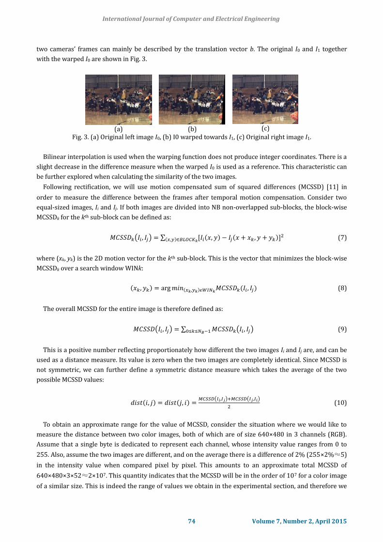
two cameras’ frames can mainly be described by the translation vector b. The original I0 and I1 together
with the warped I0 are shown in Fig. 3.
(a)
(b)
(c)
Fig. 3. (a) Original left image I0, (b) I0 warped towards I1, (c) Original right image I1.
Bilinear interpolation is used when the warping function does not produce integer coordinates. There is a
slight decrease in the difference measure when the warped I0 is used as a reference. This characteristic can
be further explored when calculating the similarity of the two images.
Following rectification, we will use motion compensated sum of squared differences (MCSSD) [11] in
order to measure the difference between the frames after temporal motion compensation. Consider two
equal-sized images, Ii and Ij. If both images are divided into NB non-overlapped sub-blocks, the block-wise
MCSSDk for the kth sub-block can be defined as:
𝑀𝐶𝑆𝑆𝐷𝑘(𝐼𝑖 , 𝐼𝑗) = ∑ [𝐼𝑖(𝑥, 𝑦) − 𝐼𝑗(𝑥 + 𝑥𝑘 , 𝑦 + 𝑦𝑘)]2(𝑥,𝑦)∈𝐵𝐿𝑂𝐶𝐾𝑘
(7)
where (xk, yk) is the 2D motion vector for the kth sub-block. This is the vector that minimizes the block-wise
MCSSDk over a search window WINk:
(𝑥𝑘, 𝑦𝑘) = arg 𝑚𝑖𝑛(𝑥𝑘,𝑦𝑘)𝜖𝑊𝐼𝑁𝑘𝑀𝐶𝑆𝑆𝐷𝑘(𝐼𝑖 , 𝐼𝑗) (8)
The overall MCSSD for the entire image is therefore defined as:
𝑀𝐶𝑆𝑆𝐷(𝐼𝑖 , 𝐼𝑗) = ∑ 𝑀𝐶𝑆𝑆𝐷𝑘(𝐼𝑖 , 𝐼𝑗)0≤𝑘≤𝑁𝐵−1 (9)
This is a positive number reflecting proportionately how different the two images Ii and Ij are, and can be
used as a distance measure. Its value is zero when the two images are completely identical. Since MCSSD is
not symmetric, we can further define a symmetric distance measure which takes the average of the two
possible MCSSD values:
𝑑𝑖𝑠𝑡(𝑖, 𝑗) = 𝑑𝑖𝑠𝑡(𝑗, 𝑖) =𝑀𝐶𝑆𝑆𝐷(𝐼𝑖,𝐼𝑗)+𝑀𝐶𝑆𝑆𝐷(𝐼𝑗,𝐼𝑖)
2 (10)
To obtain an approximate range for the value of MCSSD, consider the situation where we would like to
measure the distance between two color images, both of which are of size 640×480 in 3 channels (RGB).
Assume that a single byte is dedicated to represent each channel, whose intensity value ranges from 0 to
255. Also, assume the two images are different, and on the average there is a difference of 2% (255×2%≈5)
in the intensity value when compared pixel by pixel. This amounts to an approximate total MCSSD of
640×480×3×52≈2×10⁷. This quantity indicates that the MCSSD will be in the order of 107 for a color image
of a similar size. This is indeed the range of values we obtain in the experimental section, and therefore we
International Journal of Computer and Electrical Engineering
74 Volume 7, Number 2, April 2015

verify the validity of our measured MCSSD values. The distance measure may be larger or smaller,
depending on the actual difference that exists between the two images.
The MCSSD between (I1, I0) in Fig. 2 is 15.01, while MCSSD (I1, W1←0(I0)) is 13.83, where W1←0 (•) denotes
the warping function from the view point of Camera 0 to that of Camera 1. Therefore, we can see that
MCSSD decreases after the warping operation as a result of revealing the hidden similarities.
Instead of manually specifying feature points on the images, an alternative is to use Scale Invariant
Feature Transform (SIFT) descriptors [13]. The detected SIFT features of I2 and I3 at t=47 are shown in Fig.
4(a) and (b), respectively. The correspondence between the feature points of the two images can be
obtained using a search procedure based on kd-tree. The matching of 146 feature points is shown in Fig.
4(c). The coordinates of these corresponding feature points can then be substituted into both sides of (4) to
solve the transformation matrix A. In this case, A is found to be:
𝐴3⟵2,47 = [1.020522 0.044407 −5.6013400.001055 1.006317 −2.324421
] (11)
(a)
(c)
(b)
Fig. 4. (a) SIFT features of I2; (b) SIFT features of I3; (c) matching features.
Once again, we can observe that a is very close to an identity matrix, as all cameras are in a 1D linear
arrangement. In addition, A3←2,47 is slightly different than A1←0,0 because the video contents are different.
3.2. Finding the Proper Compression Sequence
After measuring the similarity between the videos, the next step is to define the best sequence of
compression that achieves the highest compression rate (least amount of redundancy). In order to find the
best encoding order, we model the problem as a graph traversal problem where each camera is a node and
the weight of the edges connecting two nodes is defined to be the distance of the frames that they record:
𝑤𝑖𝑗 = 𝑑𝑖𝑠𝑡(𝑖, 𝑗) = 𝑑𝑖𝑠𝑡(𝑗, 𝑖) = 𝑤𝑗𝑖 (12)
where wij refers to the weight between camera i and j. The best camera traversal order maximizing the
International Journal of Computer and Electrical Engineering
75 Volume 7, Number 2, April 2015
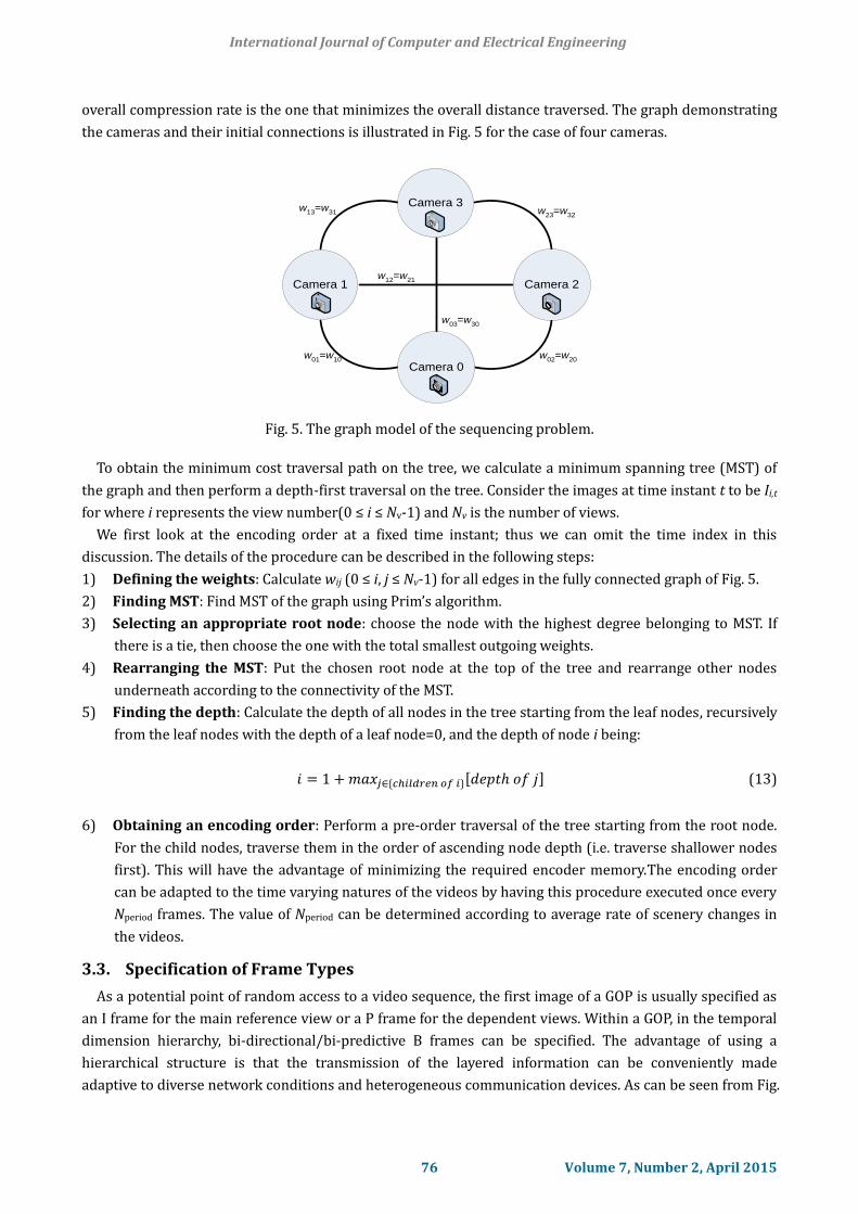
overall compression rate is the one that minimizes the overall distance traversed. The graph demonstrating
the cameras and their initial connections is illustrated in Fig. 5 for the case of four cameras.
w01
=w10
w02
=w20
w12
=w21
w13
=w31 w
23=w
32
w03
=w30
Camera 0
Camera 1 Camera 2
Camera 3
Fig. 5. The graph model of the sequencing problem.
To obtain the minimum cost traversal path on the tree, we calculate a minimum spanning tree (MST) of
the graph and then perform a depth-first traversal on the tree. Consider the images at time instant t to be Ii,t
for where i represents the view number(0 ≤ i ≤ Nv-1) and Nv is the number of views.
We first look at the encoding order at a fixed time instant; thus we can omit the time index in this
discussion. The details of the procedure can be described in the following steps:
1) Defining the weights: Calculate wij (0 ≤ i, j ≤ Nv-1) for all edges in the fully connected graph of Fig. 5.
2) Finding MST: Find MST of the graph using Prim’s algorithm.
3) Selecting an appropriate root node: choose the node with the highest degree belonging to MST. If
there is a tie, then choose the one with the total smallest outgoing weights.
4) Rearranging the MST: Put the chosen root node at the top of the tree and rearrange other nodes
underneath according to the connectivity of the MST.
5) Finding the depth: Calculate the depth of all nodes in the tree starting from the leaf nodes, recursively
from the leaf nodes with the depth of a leaf node=0, and the depth of node i being:
𝑖 = 1 + 𝑚𝑎𝑥𝑗∈{𝑐ℎ𝑖𝑙𝑑𝑟𝑒𝑛 𝑜𝑓 𝑖}[𝑑𝑒𝑝𝑡ℎ 𝑜𝑓 𝑗] (13)
6) Obtaining an encoding order: Perform a pre-order traversal of the tree starting from the root node.
For the child nodes, traverse them in the order of ascending node depth (i.e. traverse shallower nodes
first). This will have the advantage of minimizing the required encoder memory.The encoding order
can be adapted to the time varying natures of the videos by having this procedure executed once every
Nperiod frames. The value of Nperiod can be determined according to average rate of scenery changes in
the videos.
3.3. Specification of Frame Types
As a potential point of random access to a video sequence, the first image of a GOP is usually specified as
an I frame for the main reference view or a P frame for the dependent views. Within a GOP, in the temporal
dimension hierarchy, bi-directional/bi-predictive B frames can be specified. The advantage of using a
hierarchical structure is that the transmission of the layered information can be conveniently made
adaptive to diverse network conditions and heterogeneous communication devices. As can be seen from Fig.
International Journal of Computer and Electrical Engineering
76 Volume 7, Number 2, April 2015
7, each frame in the sequence is assigned a label and a layer number. Frames with a label of capital letter (I,
P, B) are those which will be used as reference frames during encoding/decoding, while frames with a small
letter label will not. The layer number for a frame can be used for synchronization: it can be specified that
the encoding/decoding of all the frames in one layer be completed before processing of the next
hierarchical layer is started. Merkle et al. [2] empirically show that immediate neighbors provide most of
the correlation for motion and disparity compensations. As a result, we only consider frames that are in
adjacent proximity to a frame. Given several candidate reference frames available in the reference list
during the encoding of a macro-block k, we choose the reference frame which minimizes the Lagrangian
rate distortion cost as follows:
𝑚𝑖𝑛𝐹𝑅∈{𝑅𝑒𝑓 𝐿𝑖𝑠𝑡}[𝑀𝐶𝑆𝑆𝐷𝑘(𝐹𝑅) + 𝜆𝑚𝑜𝑡𝑖𝑜𝑛 ⋅ 𝑅𝑚𝑜𝑡𝑖𝑜𝑛(𝑚𝑘)] (14)
where FR is a reference image frame, λmotion is the Lagrangian parameter, and Rmotion is the number of bits
required to transmit the motion vector mk=(xk, yk).
4. Experimental Evaluation
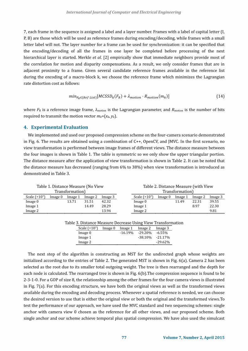
We implemented and used our proposed compression scheme on the four-camera scenario demonstrated
in Fig. 6. The results are obtained using a combination of C++, OpenCV, and JMVC. In the first scenario, no
view transformation is performed between image frames of different views. The distance measure between
the four images is shown in Table 1. The table is symmetric so we only show the upper triangular portion.
The distance measure after the application of view transformation is shown in Table 2. It can be noted that
the distance measure has decreased (ranging from 6% to 38%) when view transformation is introduced as
demonstrated in Table 3.
Table 1. Distance Measure (No View Transformation)
Scale (×107) Image 0 Image 1 Image 2 Image 3 Image 0 13.71 31.51 42.32 Image 1 14.49 28.29
Image 2 13.94
Table 2. Distance Measure (with View Transformation)
Scale (×107) Image 0 Image 1 Image 2 Image 3 Image 0 11.49 22.31 39.55 Image 1 8.97 22.30
Image 2 9.81
Table 3. Distance Measure Decrease Using View Transformation Scale (×107) Image 0 Image 1 Image 2 Image 3 Image 0 -16.19% -29.20% -6.55% Image 1 -38.10% -21.17%
Image 2 -29.62%
The next step of the algorithm is constructing an MST for the undirected graph whose weights are
initialized according to the entries of Table 2. The generated MST is shown in Fig. 6(a). Camera 2 has been
selected as the root due to its smaller total outgoing weight. The tree is then rearranged and the depth for
each node is calculated. The rearranged tree is shown in Fig. 6(b).The compression sequence is found to be
2-3-1-0. For a GOP of size 8, the relationship among the other frames for the four camera views is illustrated
in Fig. 7(a). For this encoding structure, we have both the original views as well as the transformed views
available during the encoding and decoding process. Whenever a spatial reference is needed, we can choose
the desired version to use that is either the original view or both the original and the transformed views.To
test the performance of our approach, we have used the MVC standard and two sequencing schemes: single
anchor with camera view 0 chosen as the reference for all other views, and our proposed scheme. Both
single anchor and our scheme achieve temporal plus spatial compression. We have also used the simulcast
International Journal of Computer and Electrical Engineering
77 Volume 7, Number 2, April 2015
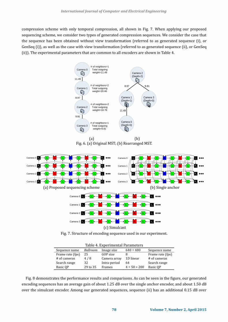
compression scheme with only temporal compression, all shown in Fig. 7. When applying our proposed
sequencing scheme, we consider two types of generated compression sequences. We consider the case that
the sequence has been obtained without view transformation (referred to as generated sequence (i), or
GenSeq (i)), as well as the case with view transformation (referred to as generated sequence (ii), or GenSeq
(ii)). The experimental parameters that are common to all encoders are shown in Table 4.
Camera 1
Camera 0
Camera 3
Camera 2
9.81
8.97
11.49
# of neighbors=1
Total outgoing
weight=11.49
# of neighbors=2
Total outgoing
weight=20.46
# of neighbors=2
Total outgoing
weight=18.78
# of neighbors=1
Total outgoing
weight=9.81
(a)
8.97
Camera 2
(Depth=2)
Camera 3
(Depth=0)
Camera 0
(Depth=0)
Camera 1
(Depth=1)
9.81
11.49
(b)
Fig. 6. (a) Original MST; (b) Rearranged MST.
Camera 3
P0
b3
B2
b3
B1
Camera 2
Camera 1
Camera 0 b3
B2
b3
P0
P0
B3
B2
B3
B1
B3
B2
B3
P0
I0
B3
B2
B3
B1
B3
B2
B3
I0
P0
b3
B2
b3
B1
b3
B2
b3
P0 Camera 3
I0
B3
B2
B3
B1
Camera 2
Camera 1
Camera 0 B3
B2
B3
I0
P0
b3
B2
b3
B1
b3
B2
b3
P0
P0
b3
B2
b3
B1
b3
B2
b3
P0
P0
b3
B2
b3
B1
b3
B2
b3
P0
(a) Proposed sequencing scheme (b) Single anchor
Camera 3
I0
b3
B2
b3
B1
Camera 2
Camera 1
Camera 0 b3
B2
b3
I0
I0
b3
B2
b3
B1
b3
B2
b3
I0
I0
b3
B2
b3
B1
b3
B2
b3
I0
I0
b3
B2
b3
B1
b3
B2
b3
I0
(c) Simulcast
Fig. 7. Structure of encoding sequence used in our experiment.
Table 4. Experimental Parameters Sequence name Ballroom Image size 640 × 480 Sequence name Frame rate (fps) 25 GOP size 8 Frame rate (fps) # of cameras 4 / 8 Camera array 1D linear # of cameras
Search range 32 Intra-period 64 Search range
Basic QP 29 to 35 Frames 4 × 50 = 200 Basic QP
Fig. 8 demonstrates the performance results and comparisons. As can be seen in the figure, our generated
encoding sequences has an average gain of about 1.25 dB over the single anchor encoder, and about 1.50 dB
over the simulcast encoder. Among our generated sequences, sequence (ii) has an additional 0.15 dB over
International Journal of Computer and Electrical Engineering
78 Volume 7, Number 2, April 2015

sequence (i). A more detailed look at the data rate reduction is shown in Table 5 for a particular PSNR.
Fig. 8. Rate distortion performance of the encoding sequences.
Table 5. Data Rate Measured at Around PSNR≈37.50db Sequence Avg. PSNR of YUV Avg. bit rate/view Generated Sequence (ii) 38.12 dB 306.41 kbps Generated Sequence (i) 37.99 dB 307.56 kbps
Single Anchor 37.50 dB 397.69 kbps
Simulcast 37.46 dB 442.20 kbps
5. Conclusions
In this paper we have proposed a novel multi-view video compression scheme that achieves higher
compression by removing the rotational inter-view redundancies among video streams simultaneously
recorded from multiple views. The images captured from different views are first rectified using a
transformation and then compressed in a specific order. This order is determined by an optimal stream
encoding algorithm that is designed to enable the encoder to automatically decide on the ordering, and
finds the best reference streams. Such optimal solution is found by modeling and solving the problem as a
graph traversal problem among the camera views. Performance evaluations demonstrate the fact that the
system achieves a better compression rate compared to simulcast and single anchor compression.
References
[1] Shirmohammadi, S., Hefeeda, M., Ooi, W. S., & Grigoras, R. (2012). Introduction to special section on 3D
mobile multimedia. ACM Transactions on Multimedia Computing, Communications, and Applications,
8(3s).
[2] Merkle, P., Muller, K., Smolic, A., & Wiegand, T. (2006). Efficient compression of multi-view video
exploiting inter-view dependencies based on H.264/MPEG4-AVC. Proceedings of IEEE International
Conf. on Multimedia and Expo (pp. 1717-1720). New York, USA: IEEE.
[3] Kubota, A., Smolic, A., Magnor, M., Tanimoto, M., Chen, T., & Zhang, C. (2007). Multi-view imaging and
3DTV. IEEE Signal Processing Magazine, 24(6), 10-21.
[4] Magnor, M., Ramanathan, P., & Girod, B. (2003). Multi-view coding for image-based rendering using 3-D
scene geometry. IEEE Tran. Circuits and Systems for Video Technology, 13(11), 1092-1106.
[5] Florencio, D., & Zhang, C. (2009). Multiview video compression and streaming based on predicted
International Journal of Computer and Electrical Engineering
79 Volume 7, Number 2, April 2015
viewer position. Proceedings of IEEE International Conference on Acoustics, Speech and Signal Processing
(pp. 657-660). New York, USA: IEEE.
[6] Luo, L., Wu, Y., Li, J., & Zhang, Y.-Q. (2002). 3-D wavelet compression and progressive inverse wavelet
synthesis rendering of concentric mosaic. IEEE Trans. on Image Processing, 11(7), 802–816.
[7] Maitre, M., Shinagawa, Y., & Do, M. N. (2008). Wavelet-based joint estimation and encoding of
depth-image-based representations for free viewpoint rendering. IEEE Trans. on Image Processing,
17(6), 946–957.
[8] Li, L., & Hou, Z. (2007). Multiview video compression with 3D-DCT. Proceedings of ITI 5th Conf. on
Information and Comm. Technology (pp. 59–61). New York, USA: IEEE.
[9] Bai, B., Boulanger, P., & Harms, J. (2005). An efficient multiview video compression scheme. Proceedings
of IEEE International Conference on Multimedia and Expo (pp. 836-839). New York, USA: IEEE.
[10] Li, D.-X., Zheng, W., Xie, X.-H., & Zheng, M. (2007). Optimisinginter-view prediction structure for
multiview video coding with minimum spanning tree. Electronics Letters, 43(23), 1269-1271.
[11] Kang, J.-W., Cho, S.-H., Hur, N. H., Kim, C. S., & Lee, S. U. (2007). Graph theoretical optimization of
prediction structure in multiview video coding. Proceedings of IEEE International Conference on Image
Processing: Vol. VI (pp. 429-432). New York, USA: IEEE.
[12] Fusiello, A., Trucco, E., & Verri, A. (2000). A compact algorithm for rectification of stereo pairs. Machine
Vision and Applications, 12(1), 16-22.
[13] Hess, R. (2010). An open-source SIFT library. Proceedings of ACM Multimedia (pp. 1493-1496). New
York, USA: ACM.
Chi Wa Leong was a PhD student at the Distributed and Collaborative Virtual
Environment Research Laboratory (DISCOVER Lab), University of Ottawa, Canada, from
2009 to 2011. His research was focused on telepresence systems and networks,
3D/multiview video, and tele-immersive virtual environments.
Behnoosh Hariri received her PhD degree in electrical engineering from Sharif
University of Technology, Iran, in 2009, and was a MITACS elevate postdoctoral fellow at
the Distributed and Collaborative Virtual Environment Research Laboratory (DISCOVER
Lab), University of Ottawa, Canada, from 2009 to 2011. Her research was focused on
gaming systems and networks, especially massively multiuser virtual environments, as
well as vision based multimedia systems. She currently works at Google Inc. in New York,
USA.
Shervin Shirmohammadi received his PhD degree in electrical engineering from the
University of Ottawa, Canada, where he is currently a full professor at the School of
Electrical Engineering and Computer Science. He is the co-director of both the DISCOVER
Lab, and the Multimedia Communications Research Laboratory (MCRLab), conducting
research in multimedia systems and networking, specifically in gaming systems and
virtual environments, video systems, and multimedia-assisted biomedical engineering.
International Journal of Computer and Electrical Engineering
80 Volume 7, Number 2, April 2015

The results of his research have led to more than 250 publications, over 20 patents and technology transfers
to the private sector, and a number of awards and prizes. He is the associate editor-in-chief of IEEE
Instrumentation and Measurement Magazine, a senior associate editor of ACM Transactions on Multimedia
Computing, Communications, and Applications, and an associate editor of IEEE Transactions on
Instrumentation and Measurement. He had been an associate editor of Springer’s Journal of Multimedia Tools
and Applications from 2004 to 2012. He also has been chairs or serves on the program committee of a
number of conferences in multimedia, virtual environments, and games. Dr. Shirmohammadi is a University
of Ottawa gold medalist, a licensed professional engineer in Ontario, a senior member of IEEE, and a
professional member of ACM.
International Journal of Computer and Electrical Engineering
81 Volume 7, Number 2, April 2015


