Nonlinear Dyn (2010) 62: 237–251DOI 10.1007/s11071-010-9714-6

O R I G I NA L PA P E R

Experimental characterization of nonlinear systems:a real-time evaluation of the analogous Chua’s circuitbehavior

Ronilson Rocha · Guilherme L.D. Andrucioli ·Rene O. Medrano-T

Received: 15 July 2009 / Accepted: 31 March 2010 / Published online: 27 April 2010© Springer Science+Business Media B.V. 2010

Abstract This paper presents an experimental char-acterization of the behavior of an analogous version ofthe Chua’s circuit. The electronic circuit signals arecaptured using a data acquisition board (DAQ) andprocessed using LabVIEW environment. The follow-ing aspects of the time series analysis are analyzed:time waveforms, phase portraits, frequency spectra,Poincaré sections, and bifurcation diagram. The circuitbehavior is experimentally mapped with the parametervariations, where are identified equilibrium points, pe-riodic and chaotic attractors, and bifurcations. Theseanalysis techniques are performed in real-time and canbe applied to characterize, with precision, several non-linear systems.

Keywords Chaotic systems · Electronic analogy ·Nonlinear dynamics · Data acquisition · AnalogousChua’s circuit

R. Rocha (�) · G.L.D. AndrucioliFederal University of Ouro Preto—UFOP/EM/DECAT,Campus Morro do Cruzeiro, 35400-000, Ouro Preto, MG,Brazile-mail: rocha@em.ufop.br

G.L.D. Andruciolie-mail: guilhermeandrucioli@yahoo.com.br

R.O. Medrano-TUniversity of São Paulo—USP/Institute of Physics,C-P: 66318, 05508-900, São Paulo, SP, Brazile-mail: rmedrano@if.usp.br

1 Introduction

Chaotic systems present an unpredictability behav-ior extremely sensitive to parameters variations andinitial conditions, although they are completely de-scribed by deterministic laws and nonlinear differ-ential equations without stochastic components. Thisdynamical behavior has been extensively studied bymathematicians, physicians, engineers, and more re-cently, specialists in information and social sciences,due to its great potential for commercial and indus-trial applications in areas such as engineering, infor-matics, electronics, communication, robotics, chem-istry, medicine, biology, epidemiology, management,finance, information processing, etc. [1–3]. One of themost important chaotic systems was created in 1983,an electrical circuit constituted by a network of linearpassive elements connected to a nonlinear active com-ponent, known as Chua’s diode, which standard formis shown in Fig. 1. Since its initial proposal, the Chua’scircuit is intensely investigated and has been acceptedas paradigm for study of important features of nonlin-ear systems, once it exhibits a very complex dynamicalbehavior in spite of its simplicity [4]. It still presentsa novel and rich scenario formed by a large variety ofhomoclinic orbits and bifurcations [5], periodic struc-tures [6], and distinct chaotic attractors [7].

For the experimental point of view, a characteriza-tion of dynamical behavior of a nonlinear system onlybased in computer simulations is not totally reliable,since the simulated model may only describe the sys-

238 R. Rocha et al.

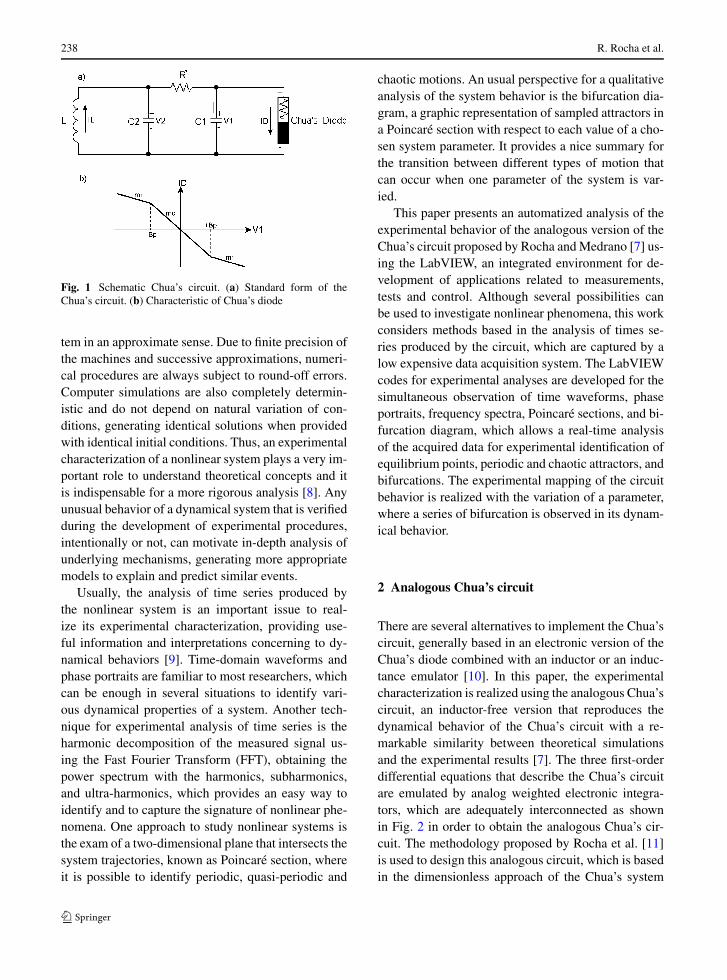
Fig. 1 Schematic Chua’s circuit. (a) Standard form of theChua’s circuit. (b) Characteristic of Chua’s diode

tem in an approximate sense. Due to finite precision ofthe machines and successive approximations, numeri-cal procedures are always subject to round-off errors.Computer simulations are also completely determin-istic and do not depend on natural variation of con-ditions, generating identical solutions when providedwith identical initial conditions. Thus, an experimentalcharacterization of a nonlinear system plays a very im-portant role to understand theoretical concepts and itis indispensable for a more rigorous analysis [8]. Anyunusual behavior of a dynamical system that is verifiedduring the development of experimental procedures,intentionally or not, can motivate in-depth analysis ofunderlying mechanisms, generating more appropriatemodels to explain and predict similar events.

Usually, the analysis of time series produced bythe nonlinear system is an important issue to real-ize its experimental characterization, providing use-ful information and interpretations concerning to dy-namical behaviors [9]. Time-domain waveforms andphase portraits are familiar to most researchers, whichcan be enough in several situations to identify vari-ous dynamical properties of a system. Another tech-nique for experimental analysis of time series is theharmonic decomposition of the measured signal us-ing the Fast Fourier Transform (FFT), obtaining thepower spectrum with the harmonics, subharmonics,and ultra-harmonics, which provides an easy way toidentify and to capture the signature of nonlinear phe-nomena. One approach to study nonlinear systems isthe exam of a two-dimensional plane that intersects thesystem trajectories, known as Poincaré section, whereit is possible to identify periodic, quasi-periodic and

chaotic motions. An usual perspective for a qualitativeanalysis of the system behavior is the bifurcation dia-gram, a graphic representation of sampled attractors ina Poincaré section with respect to each value of a cho-sen system parameter. It provides a nice summary forthe transition between different types of motion thatcan occur when one parameter of the system is var-ied.

This paper presents an automatized analysis of theexperimental behavior of the analogous version of theChua’s circuit proposed by Rocha and Medrano [7] us-ing the LabVIEW, an integrated environment for de-velopment of applications related to measurements,tests and control. Although several possibilities canbe used to investigate nonlinear phenomena, this workconsiders methods based in the analysis of times se-ries produced by the circuit, which are captured by alow expensive data acquisition system. The LabVIEWcodes for experimental analyses are developed for thesimultaneous observation of time waveforms, phaseportraits, frequency spectra, Poincaré sections, and bi-furcation diagram, which allows a real-time analysisof the acquired data for experimental identification ofequilibrium points, periodic and chaotic attractors, andbifurcations. The experimental mapping of the circuitbehavior is realized with the variation of a parameter,where a series of bifurcation is observed in its dynam-ical behavior.

2 Analogous Chua’s circuit

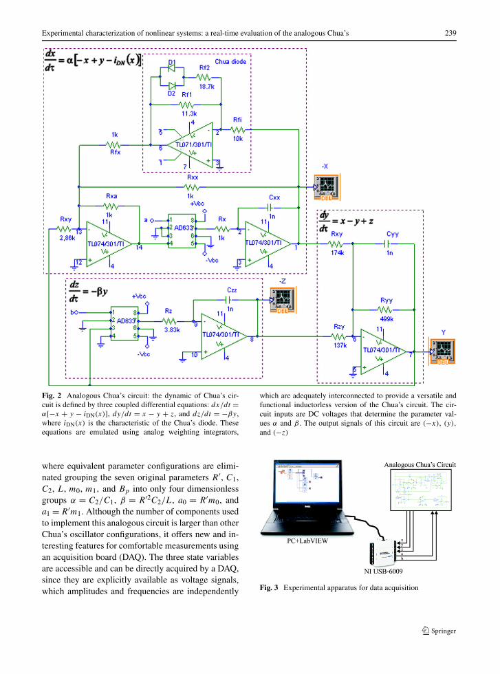
There are several alternatives to implement the Chua’scircuit, generally based in an electronic version of theChua’s diode combined with an inductor or an induc-tance emulator [10]. In this paper, the experimentalcharacterization is realized using the analogous Chua’scircuit, an inductor-free version that reproduces thedynamical behavior of the Chua’s circuit with a re-markable similarity between theoretical simulationsand the experimental results [7]. The three first-orderdifferential equations that describe the Chua’s circuitare emulated by analog weighted electronic integra-tors, which are adequately interconnected as shownin Fig. 2 in order to obtain the analogous Chua’s cir-cuit. The methodology proposed by Rocha et al. [11]is used to design this analogous circuit, which is basedin the dimensionless approach of the Chua’s system

Experimental characterization of nonlinear systems: a real-time evaluation of the analogous Chua’s 239

Fig. 2 Analogous Chua’s circuit: the dynamic of Chua’s cir-cuit is defined by three coupled differential equations: dx/dt =α[−x + y − iDN(x)], dy/dt = x − y + z, and dz/dt = −βy,where iDN(x) is the characteristic of the Chua’s diode. Theseequations are emulated using analog weighting integrators,

which are adequately interconnected to provide a versatile andfunctional inductorless version of the Chua’s circuit. The cir-cuit inputs are DC voltages that determine the parameter val-ues α and β . The output signals of this circuit are (−x), (y),

and (−z)

where equivalent parameter configurations are elimi-nated grouping the seven original parameters R′, C1,C2, L, m0, m1, and Bp into only four dimensionlessgroups α = C2/C1, β = R′2C2/L, a0 = R′m0, anda1 = R′m1. Although the number of components usedto implement this analogous circuit is larger than otherChua’s oscillator configurations, it offers new and in-teresting features for comfortable measurements usingan acquisition board (DAQ). The three state variablesare accessible and can be directly acquired by a DAQ,since they are explicitly available as voltage signals,which amplitudes and frequencies are independently Fig. 3 Experimental apparatus for data acquisition

240 R. Rocha et al.

defined in circuit design from scaling [7]. Thus, thecharacteristics of the output signals of the analogousChua’s circuit can be adjusted according to DAQ spec-ifications. Another advantage of the analogous Chua’scircuit is that the parameters α and β can be easilyvaried in a large range by external DC voltage levelsprovide by the DAQ, facilitating the automatic compu-tational analyses of the circuit. The experimental anal-

ogous Chua’s circuit is implemented using the IC’sAD633 (analog multiplier), IC TL071 (single op-amp)and IC TL074 (quad op-amp). Two red LEDs are usedin an antiparallel diodes configuration of the analo-gous Chua’s diode. The normalized dimensionless pa-rameters a = α/35 and b = β/35 are represented byexternal DC voltage levels. In this work, the parame-ter b is fixed in 3 V.

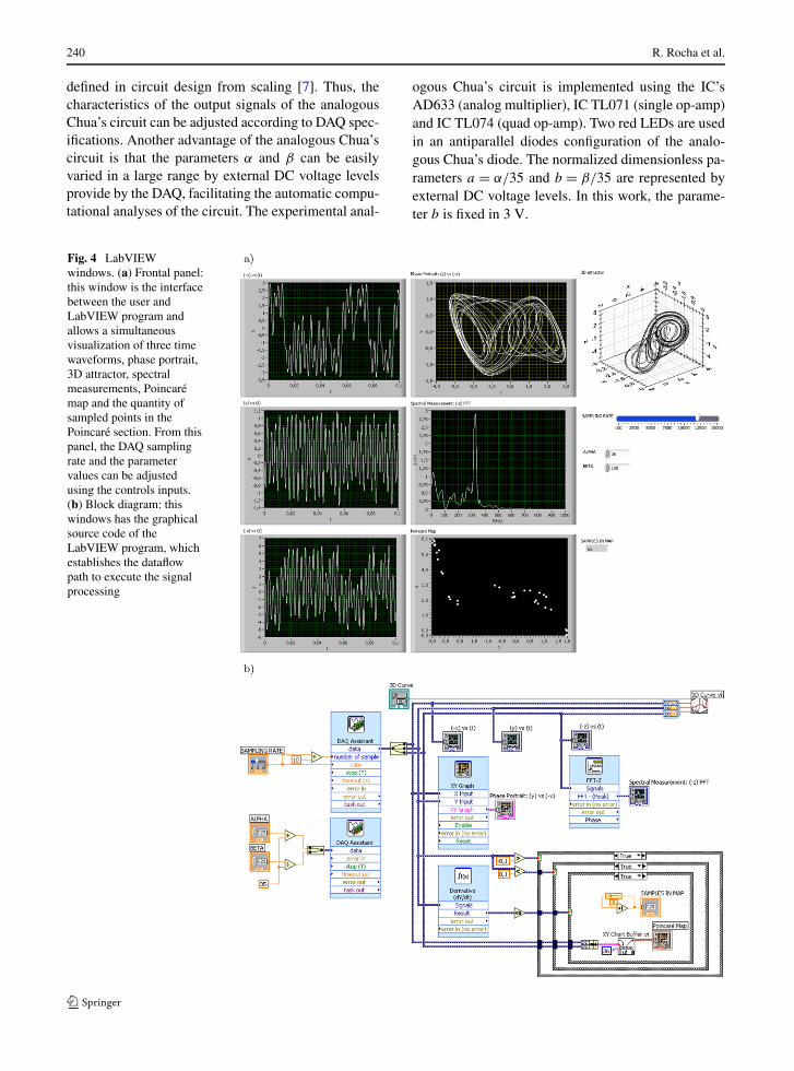
Fig. 4 LabVIEWwindows. (a) Frontal panel:this window is the interfacebetween the user andLabVIEW program andallows a simultaneousvisualization of three timewaveforms, phase portrait,3D attractor, spectralmeasurements, Poincarémap and the quantity ofsampled points in thePoincaré section. From thispanel, the DAQ samplingrate and the parametervalues can be adjustedusing the controls inputs.(b) Block diagram: thiswindows has the graphicalsource code of theLabVIEW program, whichestablishes the dataflowpath to execute the signalprocessing

Experimental characterization of nonlinear systems: a real-time evaluation of the analogous Chua’s 241

3 Data acquisition

3.1 Hardware

The experimental apparatus for data acquisition andsignal processing is presented in Fig. 3. The electri-cal signals generated by the analogous Chua’s circuitare acquired at a rate of 16 kSamples/s by three sin-gle ended analog inputs of a NI USB-6009, a USBbased data acquisition (DAQ) and control device man-ufactured by National Instruments. This DAQ has 8referenced single ended signal coupling or 4 differen-tial signal coupling analog inputs (14-bit resolution,48 kSamples/s), and 2 analog outputs (12-bit resolu-tion, 150 samples/s), which are used to generate theparameters a and b for the analogous Chua’s circuit.It has still 12 configurable digital input/output (5VTTL/CMOS) and a 32-bit counter.

3.2 Software

The real-time data analysis is realized using the Lab-oratory Virtual Instruments Engineering Workbench(LabVIEW), which is a software widely used for dataacquisition, prototyping and testing, containing a com-prehensive set of tools for acquiring, analyzing, dis-playing, and storing data. The main concepts and tech-niques for LabVIEW programming can be found inmanuals [12, 13]. The LabVIEW programming is vi-sual and uses graphical representations of functions,mathematical subroutines, displays, and other utilitiesextremely useful for data analysis and signal process-ing. Since a LabVIEW program imitates physical in-struments, it is called virtual instrument (VI) and

presents two fundamental parts as shown in Fig. 4: thefrontal panel and the block diagram.

The frontal panel is shown in Fig. 4a and consistsin the interface between the user and the VI. This win-dow is composed by controls and indicators, whichare available in the “controls palette” and consist inthe interactive inputs and outputs terminals of the VI,respectively. The controls are knobs, push, buttons,dials, and other elements that simulate inputs mech-anisms in a VI, while the indicators are the outputsmechanisms of a VI such as graphs, charts, LEDs, andother elements for visualization of signals or alarms.

The block diagram is the graphical source code ofa VI shown in Fig. 4b, which is built in a second win-dow using terminals, nodes, and wires. The terminalsare entry and exit ports that exchange information be-tween the front panel and block diagram. Thus, foreach control or indicator placed in the frontal panel, anicon terminal is inserted on the block diagram. Nodesare objects on the block diagram with inputs and/oroutputs that perform operations, which can be avail-able in the “functions palette” or created by the ownuser as another VI. The main types of nodes in Lab-VIEW are functions (statements, operators, or func-tions), sub-VIs (subroutines), Express VIs (sub-VIsdesigned to aid in common measurement tasks), andstructures (repetition loops or case statements). Termi-nals and nodes are wired to establish the flow of datain the block diagram.

In the execution of a VI, the data inserted in thefrontal panel will flow to the block diagram throughthe terminals. When a node receives all required in-puts, it executes a function, sub-VI, or structure and

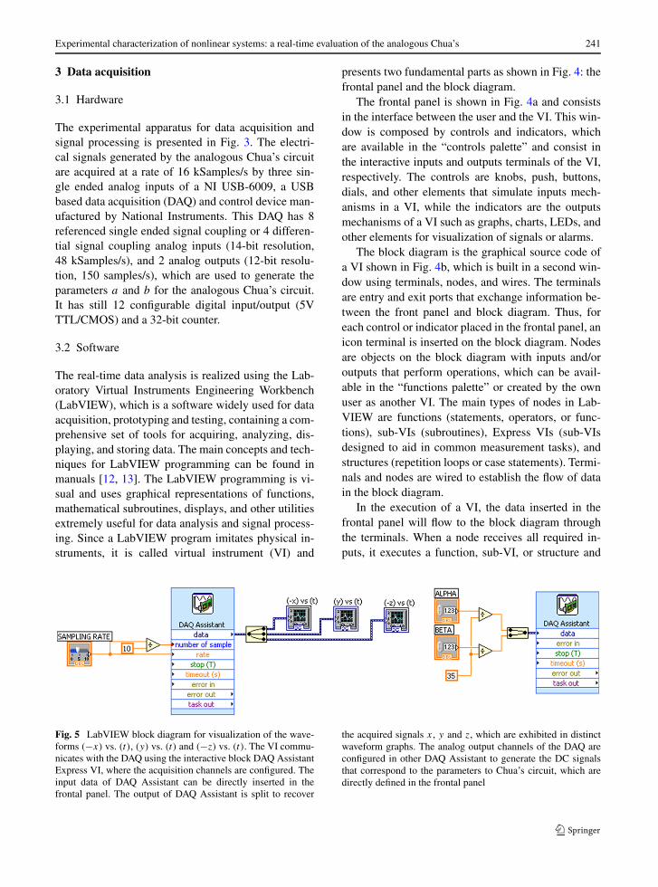
Fig. 5 LabVIEW block diagram for visualization of the wave-forms (−x) vs. (t), (y) vs. (t) and (−z) vs. (t). The VI commu-nicates with the DAQ using the interactive block DAQ AssistantExpress VI, where the acquisition channels are configured. Theinput data of DAQ Assistant can be directly inserted in thefrontal panel. The output of DAQ Assistant is split to recover

the acquired signals x, y and z, which are exhibited in distinctwaveform graphs. The analog output channels of the DAQ areconfigured in other DAQ Assistant to generate the DC signalsthat correspond to the parameters to Chua’s circuit, which aredirectly defined in the frontal panel

242 R. Rocha et al.

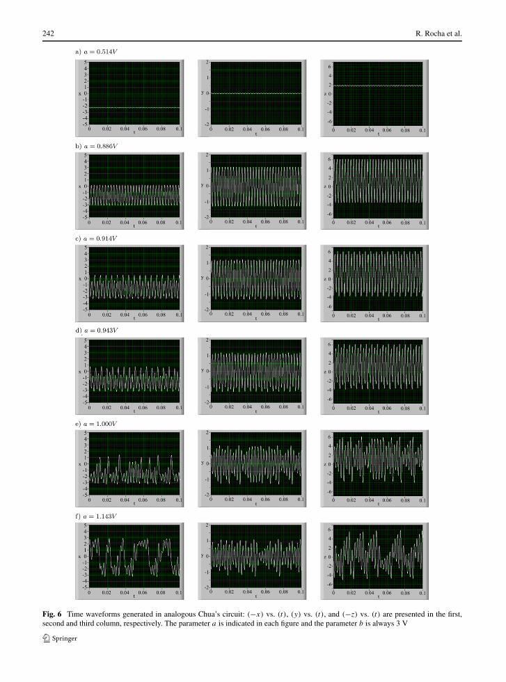
Fig. 6 Time waveforms generated in analogous Chua’s circuit: (−x) vs. (t), (y) vs. (t), and (−z) vs. (t) are presented in the first,second and third column, respectively. The parameter a is indicated in each figure and the parameter b is always 3 V

Experimental characterization of nonlinear systems: a real-time evaluation of the analogous Chua’s 243

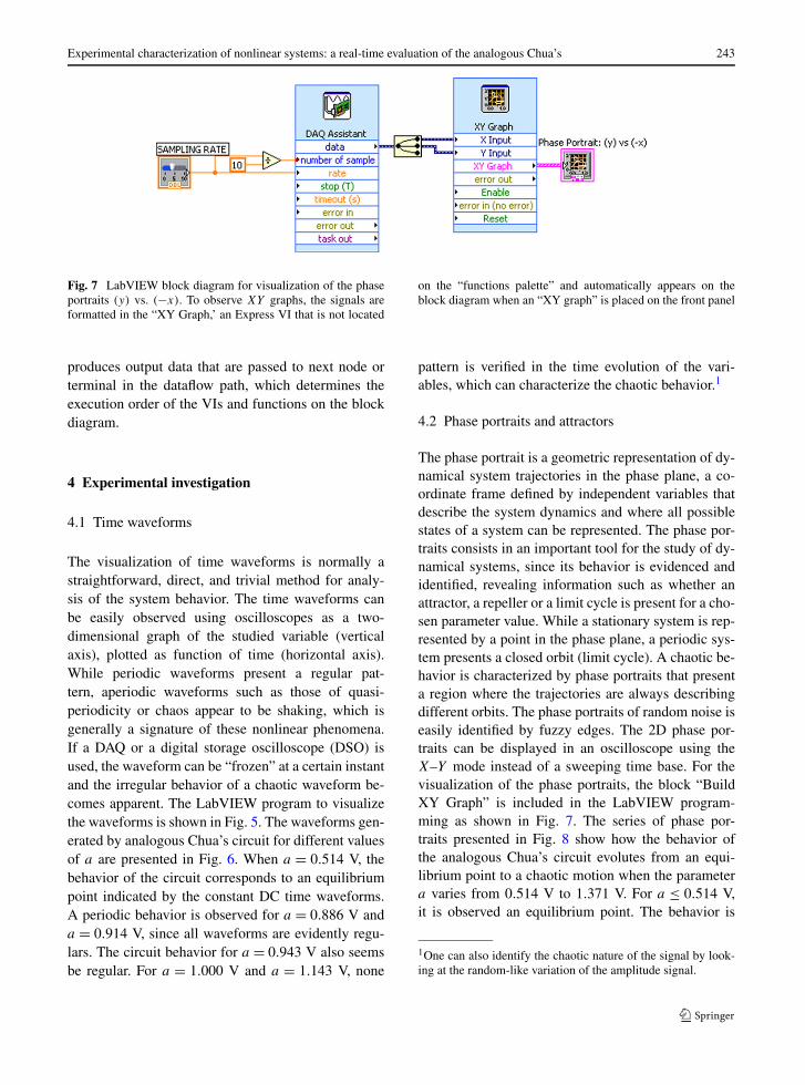
Fig. 7 LabVIEW block diagram for visualization of the phaseportraits (y) vs. (−x). To observe XY graphs, the signals areformatted in the “XY Graph,’ an Express VI that is not located

on the “functions palette” and automatically appears on theblock diagram when an “XY graph” is placed on the front panel

produces output data that are passed to next node orterminal in the dataflow path, which determines theexecution order of the VIs and functions on the blockdiagram.

4 Experimental investigation

4.1 Time waveforms

The visualization of time waveforms is normally astraightforward, direct, and trivial method for analy-sis of the system behavior. The time waveforms canbe easily observed using oscilloscopes as a two-dimensional graph of the studied variable (verticalaxis), plotted as function of time (horizontal axis).While periodic waveforms present a regular pat-tern, aperiodic waveforms such as those of quasi-periodicity or chaos appear to be shaking, which isgenerally a signature of these nonlinear phenomena.If a DAQ or a digital storage oscilloscope (DSO) isused, the waveform can be “frozen” at a certain instantand the irregular behavior of a chaotic waveform be-comes apparent. The LabVIEW program to visualizethe waveforms is shown in Fig. 5. The waveforms gen-erated by analogous Chua’s circuit for different valuesof a are presented in Fig. 6. When a = 0.514 V, thebehavior of the circuit corresponds to an equilibriumpoint indicated by the constant DC time waveforms.A periodic behavior is observed for a = 0.886 V anda = 0.914 V, since all waveforms are evidently regu-lars. The circuit behavior for a = 0.943 V also seemsbe regular. For a = 1.000 V and a = 1.143 V, none

pattern is verified in the time evolution of the vari-ables, which can characterize the chaotic behavior.1

4.2 Phase portraits and attractors

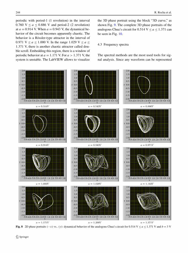
The phase portrait is a geometric representation of dy-namical system trajectories in the phase plane, a co-ordinate frame defined by independent variables thatdescribe the system dynamics and where all possiblestates of a system can be represented. The phase por-traits consists in an important tool for the study of dy-namical systems, since its behavior is evidenced andidentified, revealing information such as whether anattractor, a repeller or a limit cycle is present for a cho-sen parameter value. While a stationary system is rep-resented by a point in the phase plane, a periodic sys-tem presents a closed orbit (limit cycle). A chaotic be-havior is characterized by phase portraits that presenta region where the trajectories are always describingdifferent orbits. The phase portraits of random noise iseasily identified by fuzzy edges. The 2D phase por-traits can be displayed in an oscilloscope using theX–Y mode instead of a sweeping time base. For thevisualization of the phase portraits, the block “BuildXY Graph” is included in the LabVIEW program-ming as shown in Fig. 7. The series of phase por-traits presented in Fig. 8 show how the behavior ofthe analogous Chua’s circuit evolutes from an equi-librium point to a chaotic motion when the parametera varies from 0.514 V to 1.371 V. For a ≤ 0.514 V,it is observed an equilibrium point. The behavior is

1One can also identify the chaotic nature of the signal by look-ing at the random-like variation of the amplitude signal.

244 R. Rocha et al.

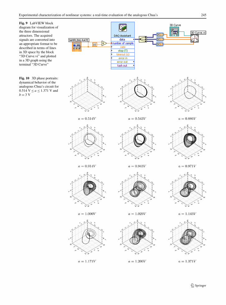
periodic with period-1 (1 revolution) in the interval0.760 V ≤ a ≤ 0.886 V and period-2 (2 revolution)at a = 0.914 V. When a = 0.943 V, the dynamical be-havior of the circuit becomes apparently chaotic. Thebehavior is a Rössler-type attractor in the interval of0.971 V ≤ a ≤ 1.000 V. In the range 1.029 V ≤ a ≤1.371 V, there is another chaotic attractor called dou-ble scroll. Embedding this region, there is a window ofperiodic behavior at a = 1.171 V. For a > 1.371 V, thesystem is unstable. The LabVIEW allows to visualize

the 3D phase portrait using the block “3D curve,” asshown Fig. 9. The complete 3D phase portraits of theanalogous Chua’s circuit for 0.514 V ≤ a ≤ 1.371 canbe seen in Fig. 10.

4.3 Frequency spectra

The spectral methods are the most used tools for sig-nal analysis. Since any waveform can be represented

Fig. 8 2D phase portraits (−x) vs.. (y): dynamical behavior of the analogous Chua’s circuit for 0.514 V ≤ a ≤ 1.371 V and b = 3 V

Experimental characterization of nonlinear systems: a real-time evaluation of the analogous Chua’s 245

Fig. 9 LabVIEW blockdiagram for visualization ofthe three dimensionalattractors. The acquiredsignals are converted intoan appropriate format to bedescribed in terms of linesin 3D space by the block“3D Curve.vi” and plottedin a 3D graph using theterminal “3D Curve”

Fig. 10 3D phase portraits:dynamical behavior of theanalogous Chua’s circuit for0.514 V ≤ a ≤ 1.371 V andb = 3 V

246 R. Rocha et al.

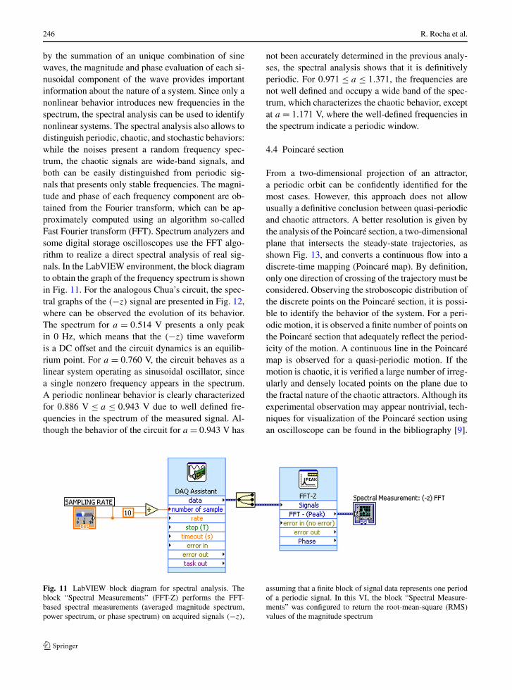
by the summation of an unique combination of sinewaves, the magnitude and phase evaluation of each si-nusoidal component of the wave provides importantinformation about the nature of a system. Since only anonlinear behavior introduces new frequencies in thespectrum, the spectral analysis can be used to identifynonlinear systems. The spectral analysis also allows todistinguish periodic, chaotic, and stochastic behaviors:while the noises present a random frequency spec-trum, the chaotic signals are wide-band signals, andboth can be easily distinguished from periodic sig-nals that presents only stable frequencies. The magni-tude and phase of each frequency component are ob-tained from the Fourier transform, which can be ap-proximately computed using an algorithm so-calledFast Fourier transform (FFT). Spectrum analyzers andsome digital storage oscilloscopes use the FFT algo-rithm to realize a direct spectral analysis of real sig-nals. In the LabVIEW environment, the block diagramto obtain the graph of the frequency spectrum is shownin Fig. 11. For the analogous Chua’s circuit, the spec-tral graphs of the (−z) signal are presented in Fig. 12,where can be observed the evolution of its behavior.The spectrum for a = 0.514 V presents a only peakin 0 Hz, which means that the (−z) time waveformis a DC offset and the circuit dynamics is an equilib-rium point. For a = 0.760 V, the circuit behaves as alinear system operating as sinusoidal oscillator, sincea single nonzero frequency appears in the spectrum.A periodic nonlinear behavior is clearly characterizedfor 0.886 V ≤ a ≤ 0.943 V due to well defined fre-quencies in the spectrum of the measured signal. Al-though the behavior of the circuit for a = 0.943 V has

not been accurately determined in the previous analy-ses, the spectral analysis shows that it is definitivelyperiodic. For 0.971 ≤ a ≤ 1.371, the frequencies arenot well defined and occupy a wide band of the spec-trum, which characterizes the chaotic behavior, exceptat a = 1.171 V, where the well-defined frequencies inthe spectrum indicate a periodic window.

4.4 Poincaré section

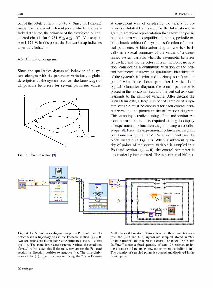
From a two-dimensional projection of an attractor,a periodic orbit can be confidently identified for themost cases. However, this approach does not allowusually a definitive conclusion between quasi-periodicand chaotic attractors. A better resolution is given bythe analysis of the Poincaré section, a two-dimensionalplane that intersects the steady-state trajectories, asshown Fig. 13, and converts a continuous flow into adiscrete-time mapping (Poincaré map). By definition,only one direction of crossing of the trajectory must beconsidered. Observing the stroboscopic distribution ofthe discrete points on the Poincaré section, it is possi-ble to identify the behavior of the system. For a peri-odic motion, it is observed a finite number of points onthe Poincaré section that adequately reflect the period-icity of the motion. A continuous line in the Poincarémap is observed for a quasi-periodic motion. If themotion is chaotic, it is verified a large number of irreg-ularly and densely located points on the plane due tothe fractal nature of the chaotic attractors. Although itsexperimental observation may appear nontrivial, tech-niques for visualization of the Poincaré section usingan oscilloscope can be found in the bibliography [9].

Fig. 11 LabVIEW block diagram for spectral analysis. Theblock “Spectral Measurements” (FFT-Z) performs the FFT-based spectral measurements (averaged magnitude spectrum,power spectrum, or phase spectrum) on acquired signals (−z),

assuming that a finite block of signal data represents one periodof a periodic signal. In this VI, the block “Spectral Measure-ments” was configured to return the root-mean-square (RMS)values of the magnitude spectrum

Experimental characterization of nonlinear systems: a real-time evaluation of the analogous Chua’s 247

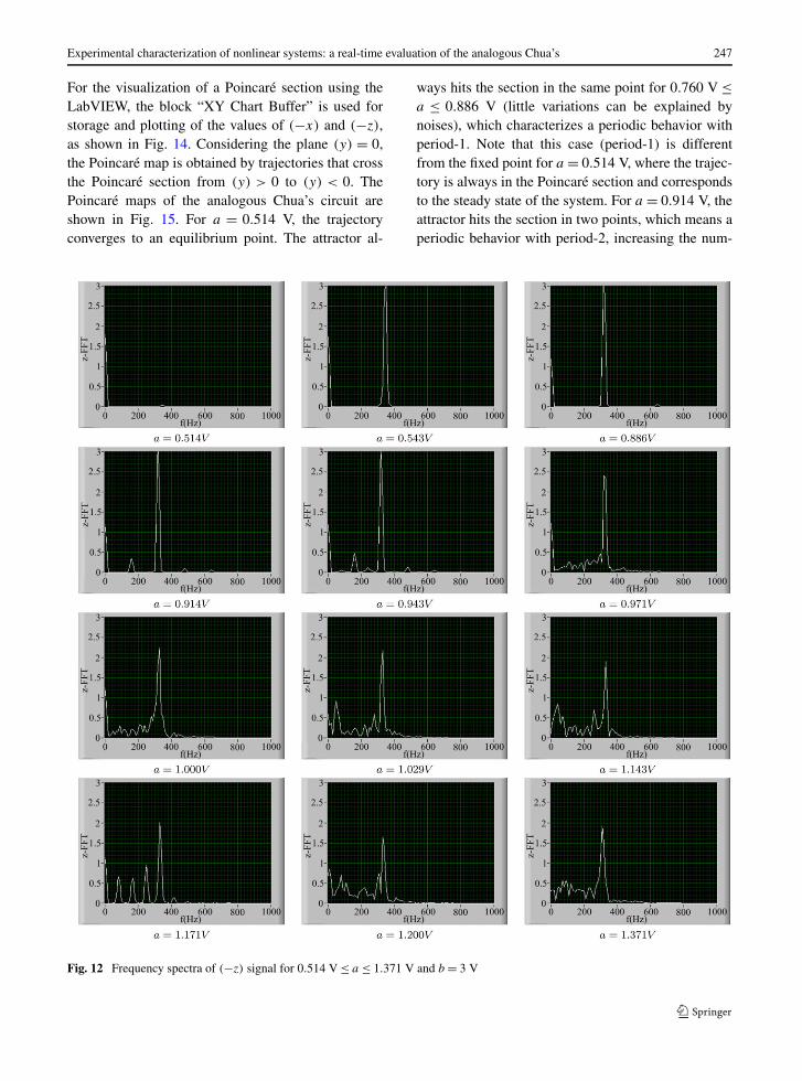
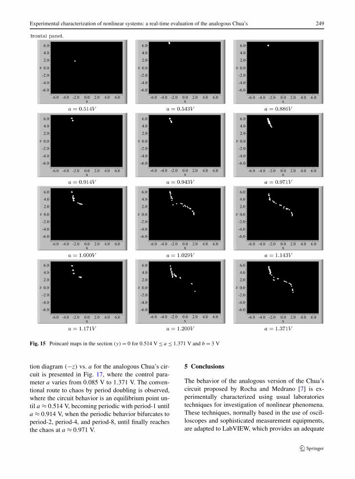
For the visualization of a Poincaré section using theLabVIEW, the block “XY Chart Buffer” is used forstorage and plotting of the values of (−x) and (−z),as shown in Fig. 14. Considering the plane (y) = 0,the Poincaré map is obtained by trajectories that crossthe Poincaré section from (y) > 0 to (y) < 0. ThePoincaré maps of the analogous Chua’s circuit areshown in Fig. 15. For a = 0.514 V, the trajectoryconverges to an equilibrium point. The attractor al-

ways hits the section in the same point for 0.760 V ≤a ≤ 0.886 V (little variations can be explained bynoises), which characterizes a periodic behavior withperiod-1. Note that this case (period-1) is differentfrom the fixed point for a = 0.514 V, where the trajec-tory is always in the Poincaré section and correspondsto the steady state of the system. For a = 0.914 V, theattractor hits the section in two points, which means aperiodic behavior with period-2, increasing the num-

Fig. 12 Frequency spectra of (−z) signal for 0.514 V ≤ a ≤ 1.371 V and b = 3 V

248 R. Rocha et al.

ber of the orbits until a = 0.943 V. Since the Poincarémap presents several different points which are irregu-larly distributed, the behavior of the circuit can be con-sidered chaotic for 0.971 V ≤ a ≤ 1.371 V, except ata = 1.171 V. In this point, the Poincaré map indicatesa periodic behavior.

4.5 Bifurcation diagrams

Since the qualitative dynamical behavior of a sys-tem changes with the parameter variations, a globaldescription of the system involves the knowledge ofall possible behaviors for several parameter values.

Fig. 13 Poincaré section [9]

A convenient way of displaying the variety of be-haviors exhibited by a system is the bifurcation dia-gram, a graphical representation that shows the possi-ble long-term values (equilibrium points, periodic or-bits, chaotic orbits) of a system as function of a con-trol parameter. A bifurcation diagram consists basi-cally in a visual summary of the values of a deter-mined system variable when the asymptotic behavioris reached and the trajectory hits in the Poincaré sec-tion, considering a continuous variation of the con-trol parameter. It allows an qualitative identificationof the system’s behavior and its changes (bifurcationpoints) when some chosen parameter is varied. In atypical bifurcation diagram, the control parameter isplaced in the horizontal axis and the vertical axis cor-responds to the sampled variable. After discard theinitial transients, a large number of samples of a sys-tem variable must be captured for each control para-meter value, and plotted in the bifurcation diagram.This sampling is realized using a Poincaré section. Anextra electronic circuit is required aiming to displayan experimental bifurcation diagram using an oscillo-scope [9]. Here, the experimental bifurcation diagramis obtained using the LabVIEW environment (see theblock diagram in Fig. 16). When a sufficient quan-tity of points of the system variable is sampled in aPoincaré section ((y) = 0), the control parameter isautomatically incremented. The experimental bifurca-

Fig. 14 LabVIEW block diagram to plot a Poincaré map. Todetect when a trajectory hits in the Poincaré section (y) = 0,two conditions are tested using case structures: (y) > −ε and(y) < ε. The more inner case structure verifies the conditiond(y)/dt < 0 to determine if the trajectory crosses the Poincarésection in direction positive to negative (y). The time deriv-ative of the (y) signal is computed using the “Time Domain

Math” block (Derivative dY/dt ). When all these conditions aretrue, the (−x) and (−z) signals are sampled, stored in “XYChart Buffer.vi” and plotted in a chart. The block “XY ChartBuffer.vi” stores a fixed quantity of data (36 points), updat-ing the more old points by new points when the buffer is full.The quantity of sampled points is counted and displayed in thefrontal panel

Experimental characterization of nonlinear systems: a real-time evaluation of the analogous Chua’s 249

Fig. 15 Poincaré maps in the section (y) = 0 for 0.514 V ≤ a ≤ 1.371 V and b = 3 V

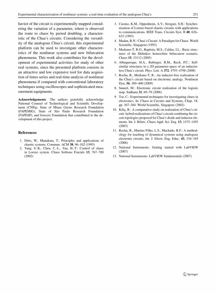
tion diagram (−z) vs. a for the analogous Chua’s cir-cuit is presented in Fig. 17, where the control para-meter a varies from 0.085 V to 1.371 V. The conven-tional route to chaos by period doubling is observed,where the circuit behavior is an equilibrium point un-til a ≈ 0.514 V, becoming periodic with period-1 untila ≈ 0.914 V, when the periodic behavior bifurcates toperiod-2, period-4, and period-8, until finally reachesthe chaos at a ≈ 0.971 V.

5 Conclusions

The behavior of the analogous version of the Chua’scircuit proposed by Rocha and Medrano [7] is ex-perimentally characterized using usual laboratoriestechniques for investigation of nonlinear phenomena.These techniques, normally based in the use of oscil-loscopes and sophisticated measurement equipments,are adapted to LabVIEW, which provides an adequate

250 R. Rocha et al.

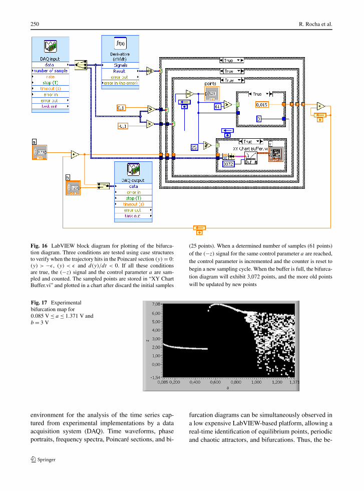
Fig. 16 LabVIEW block diagram for plotting of the bifurca-tion diagram. Three conditions are tested using case structuresto verify when the trajectory hits in the Poincaré section (y) = 0:(y) > −ε, (y) < ε and d(y)/dt < 0. If all these conditionsare true, the (−z) signal and the control parameter a are sam-pled and counted. The sampled points are stored in “XY ChartBuffer.vi” and plotted in a chart after discard the initial samples

(25 points). When a determined number of samples (61 points)of the (−z) signal for the same control parameter a are reached,the control parameter is incremented and the counter is reset tobegin a new sampling cycle. When the buffer is full, the bifurca-tion diagram will exhibit 3,072 points, and the more old pointswill be updated by new points

Fig. 17 Experimentalbifurcation map for0.085 V ≤ a ≤ 1.371 V andb = 3 V

environment for the analysis of the time series cap-tured from experimental implementations by a dataacquisition system (DAQ). Time waveforms, phaseportraits, frequency spectra, Poincaré sections, and bi-

furcation diagrams can be simultaneously observed ina low expensive LabVIEW-based platform, allowing areal-time identification of equilibrium points, periodicand chaotic attractors, and bifurcations. Thus, the be-

Experimental characterization of nonlinear systems: a real-time evaluation of the analogous Chua’s 251

havior of the circuit is experimentally mapped consid-ering the variation of a parameter, where is observedthe route to chaos by period doubling, a character-istic of the Chua’s circuits. Considering the versatil-ity of the analogous Chua’s circuit, this experimentalplatform can be used to investigate other character-istics of the nonlinear systems and new bifurcationphenomena. This work also contributes for the devel-opment of experimental activities for study of otherreal systems, since the presented platform consists inan attractive and low expensive tool for data acquisi-tion of times series and real-time analysis of nonlinearphenomena if compared with conventional laboratorytechniques using oscilloscopes and sophisticated mea-surement equipments.

Acknowledgements The authors gratefully acknowledgeNational Counsel of Technological and Scientific Develop-ment (CNPq), State of Minas Gerais Research Foundation(FAPEMIG), State of São Paulo Research Foundation(FAPESP), and Gorceix Foundation that contributed to the de-velopment of this project.

References

1. Ditto, W., Munakata, T.: Principles and applications ofchaotic systems. Commun. ACM 38, 96–102 (1995)

2. Yang, S.-K., Chen, C.-L., Yau, H.-T.: Control of chaosin Lorenz system. Chaos Solitons Fractals 13, 767–780(2002)

3. Cuomo, K.M., Oppenheim, A.V., Strogatz, S.H.: Synchro-nization of Lorenz-based chaotic circuits with applicationsto communications. IEEE Trans. Circuits Syst. II 40, 626–633 (1993)

4. Madan, R.N.: Chua’s Circuit: A Paradigm for Chaos. WorldScientific, Singapore (1993)

5. Medrano-T, R.O., Baptista, M.S., Caldas, I.L.: Basic struc-tures of the Shilnikov homoclinic bifurcation scenario.Chaos 15, 33112 (2005)

6. Albuquerque, H.A., Rubinger, R.M., Rech, P.C.: Self-similar structures in a 2D parameter-space of an inductor-less Chua’s circuit. Phys. Lett. A 372, 4793–4798 (2008)

7. Rocha, R., Medrano-T, R.: An inductor-free realization ofthe Chua’s circuit based on electronic analogy. NonlinearDyn. 56, 389–400 (2009)

8. Suneel, M.: Electronic circuit realization of the logisticmap. Sadhana 31, 69–78 (2006)

9. Tse, C.: Experimental techniques for investigating chaos inelectronics. In: Chaos in Circuits and Systems, Chap. 18,pp. 367–384. World Scientific, Singapore (2002)

10. Kiliç, R.: A comparative study on realization of Chua’s cir-cuit: hybrid realizations of Chua’s circuit combining the cir-cuit topologies proposed for Chua’s diode and inductor ele-ments. Int. J. Bifurc. Chaos Appl. Sci. Eng. 13, 1475–1493(2003)

11. Rocha, R., Martins Filho, L.S., Machado, R.F.: A method-ology for teaching of dynamical systems using analogouselectronic circuits. Int. J. Electr. Eng. Educ. 43, 334–345(2006)

12. National Instruments: Getting started with LabVIEW(2007)

13. National Instruments: LabVIEW fundamentals (2007)