
Examining Potential Demand of Public Transit for Commuting Trips
Xiaobai Yao
Department of Geography
University of Georgia, USA5 July 2006

Outline
• The trend of public transit in the US
• Objectives of the study
• Methodology
• Case study
• Conclusions
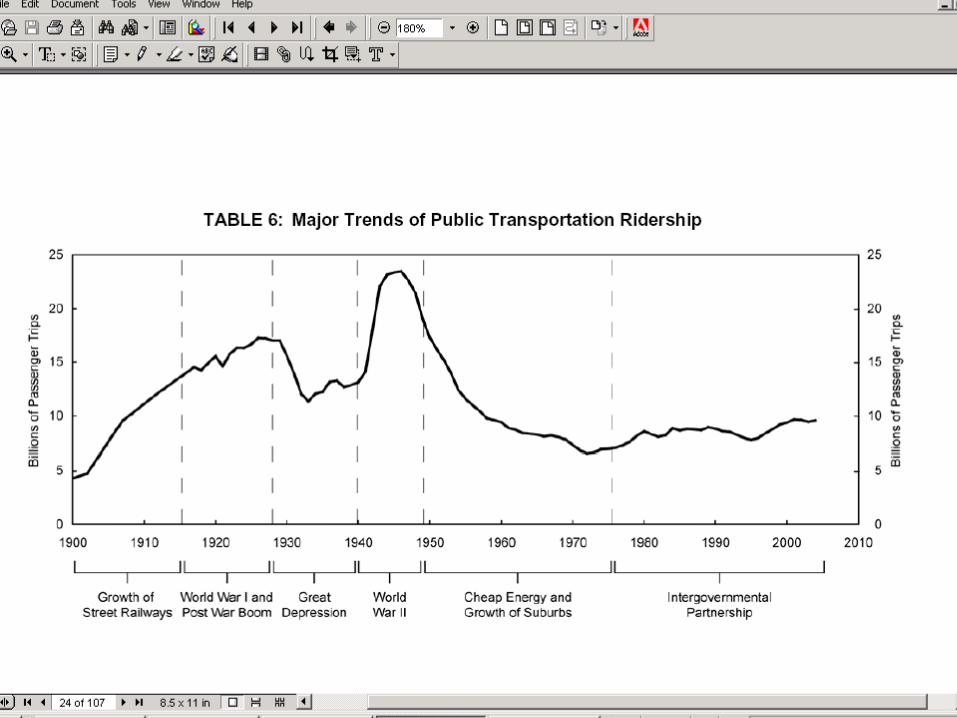


Renaissance of Public Transit in the US
• Traffic congestion
• Economic growth
• Gas price vs affordable transit fare
• Environment sustainability

Public transit networks in the city of Atlanta

Research on Public Transportation
• Accessibility for special groups
• Land use / transportation relationship
• Cost, benefit, pricing
• Network analysis
• …?

Research objectives of the study
• Measure the potential need of public transportation
• Identify and visualize clusters of high potential needs areas

Methodology
• Identify Predictive Factors
• Identifying and Visualizing Potential Demand Distribution– The Need Index approach– A data mining approach
• Case study

Data
Land-use, socioeconomic, and transportation (trips by mode) data at TAZ level.

Identify Predictive Factors
k
iiivR
1
where R is the proportion of workers taking public transit as the primary mode, vi ’s are the identified independent variables, and k is the total number of these variables.
Multiple Regression

Identify Predictive Factors- the Atlanta case
Independent variables:
• Land-use characteristics– Population density - Average number of workers per HH
– Employment rate - Job density– Percentage of home workers
• Socioeconomic characteristics– Income - Car ownership
• Network structure – Density of bus stops in the TAZ - Density of rail stations in TAZ

Predictive Variables
(Unstandardized) Coefficients Sig. Collinearity Statistics
B Std. Error Tolerance VIF
(Constant) 1.334 .824 .106
Percentage of home workers
.008 .034 .816 .864 1.157
Percentage of workers below poverty line (x1)
.074 .019 .000 .629 1.589
Percentage of workers with income from 100% to 150% of poverty line (x2)
.103 .026 .000 .679 1.474
Percentage of worker with 0 vehicle in the household (x3)
.421 .017 .000 .510 1.961
Percentage of worker with 1 vehicle in the household (x4)
.033 .010 .001 .552 1.812
Employment rate (x5) -.045 .014 .001 .541 1.847
Average # of workers per household -.007 .512 .989 .551 1.816
Population Density (x6) .036 .006 .000 .632 1.583
Job Density (x7) -.026 .002 .000 .336 2.974
Rail station Density .098 .198 .623 .832 1.201
Bus stop Density .080 .006 .000 .251 3.982
Regression Results

Identifying and Visualizing Potential Demand Distribution
1. The Need Index approach
2. A data mining approach – self-organizing maps

1. The Need Index approach
m
iii
n
iii yxR
11
yi ’s: variables accounting for the network structure and level of service of transit systems
xi ’s: variables that are not about the transit systems.
R = NI + Net
NI = R-Net
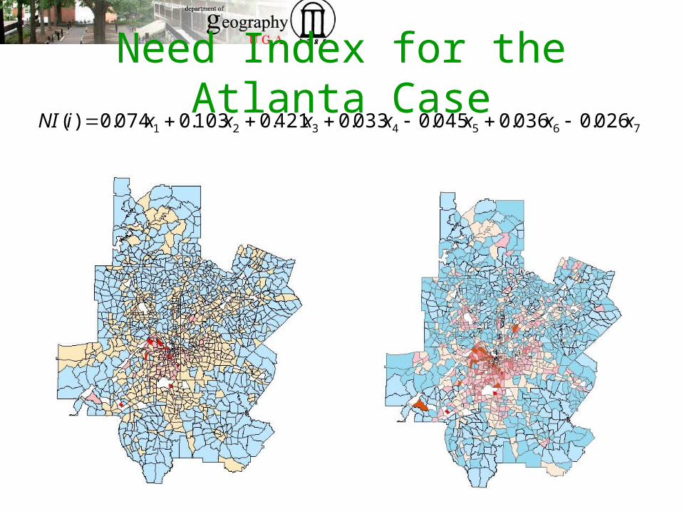
Need Index for the Atlanta Case7654321 026.0036.0045.0033.0421.0103.0074.0)( xxxxxxxiNI

Critique on the Need-Index approach
• Simple calculation• Easy interpretation • Possible to rank
and/or to quantify the difference
• Classification/Visualization Dilemma (where are the magic breaks)
• The validity of linear relationship assumption

2. The SDM approach : Self-organizing maps
<x1, x2, …. xn>

Self-organizing maps: how it works
N
jijij twtyd
1
2))()((
))()1()(()()1( twtxttwtw ijiijij

SOM in this study(weighted vector space )
nnxxx ...,, 2211
nnxxx ...,, 2211

7 8 9
4 5 6
1 2 3

Visualizing the SOM patterns


Critiques on the SOM approach
• No assumption on the relationship
• Self-assigned clusters
• No quantitative measure
• No ranking

Conclusions
• The integrative approach is successful.
• The Need Index approach and the spatial data mining approach are complementary and mutually confirmative.
• Confirmed by the other approach, the Need Index approach provides an efficient and effective solution to transportation planners.


