
Euclidean Curve Theory
by Rolf Sulanke
Finished July 28, 2009
Revised October 7, 2016
Mathenatica v. 11.0.1.0
◼ Summary
In this notebook we develop Mathematica tools for the Euclidean
differential geometry of curves. We construct Modules for the calculation
of all Euclidean invariants like arc length, curvatures, and Frenet formulas
in the plane, the 3-space, and in n-dimensional Euclidean spaces. As an
application we show that the curves of constant curvatures in the 4-
dimensional Euclidean space are isogonal trajectories of certain circular
tori and visualize them by stereographic projection. A short presentation
of Euclidean curve theory as it is used in the present notebook is given in
my paper [ECG] which may be downloaded from my homepage. In the
book [G06], see also [G94], Alfred Gray presented Euclidean differential
geometry with many applications of Mathematica. I am very much obliged
to Alfred Gray who already in 1988 introduced me in the program Wolfram
Mathematica. Many thanks also to Michael Trott for valuable hints
improving the effectivity of the symbolic calculations contained in this
notebook.
At the revision of this notebook we added subsection 4.5 about osculating
circles and osculating spheres of a curve in the Euclidean space. We tested
the notebook with Mathematica v. 9, v. 10, v.11.0.1.
◼ Keywords
curve, smooth, regular, singular, motion, velocity, arc length, tangent,
binormal, principal normal, Frenet formulas, curvatures, torsion, graph,
osculating circle, osculating sphere, helix, spiral, 1-parameter motion
group, orbits, torus, isogonal trajectory.
◼ Copyright
Initialization
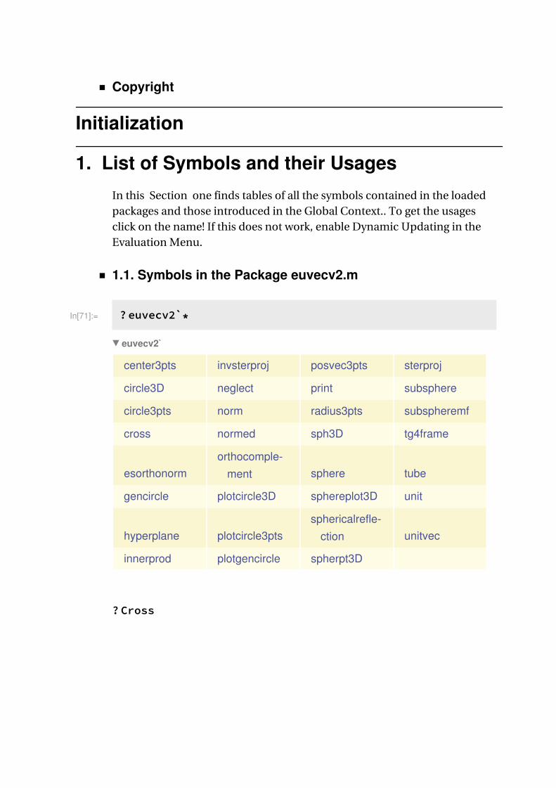
1. List of Symbols and their Usages
In this Section one finds tables of all the symbols contained in the loaded
packages and those introduced in the Global Context.. To get the usages
click on the name! If this does not work, enable Dynamic Updating in the
Evaluation Menu.
◼ 1.1. Symbols in the Package euvecv2.m
In[71]:= ?euvecv2`*
euvecv2`
center3pts invsterproj posvec3pts sterproj
circle3D neglect print subsphere
circle3pts norm radius3pts subspheremf
cross normed sph3D tg4frame
esorthonorm
orthocomple-
ment sphere tube
gencircle plotcircle3D sphereplot3D unit
hyperplane plotcircle3pts
sphericalrefle-
ction unitvec
innerprod plotgencircle spherpt3D
?Cross
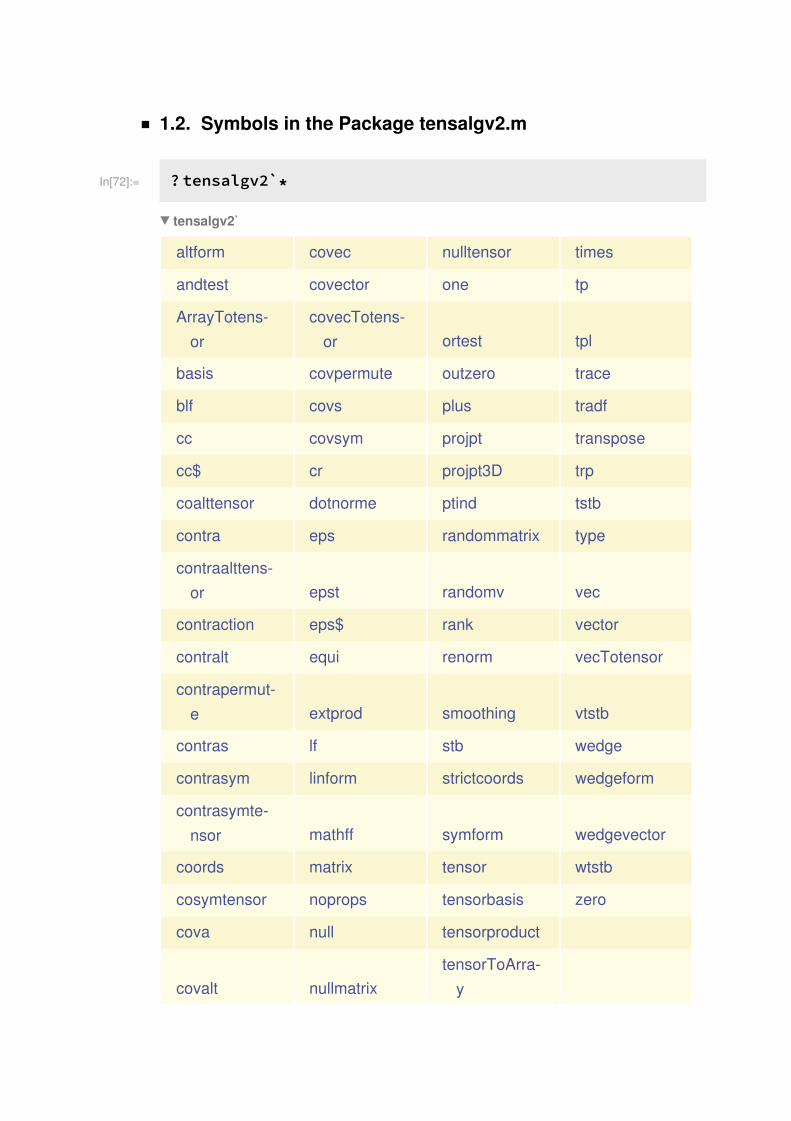
◼ 1.2. Symbols in the Package tensalgv2.m
In[72]:= ?tensalgv2`*
tensalgv2`
altform covec nulltensor times
andtest covector one tp
ArrayTotens-
or
covecTotens-
or ortest tpl
basis covpermute outzero trace
blf covs plus tradf
cc covsym projpt transpose
cc$ cr projpt3D trp
coalttensor dotnorme ptind tstb
contra eps randommatrix type
contraalttens-
or epst randomv vec
contraction eps$ rank vector
contralt equi renorm vecTotensor
contrapermut-
e extprod smoothing vtstb
contras lf stb wedge
contrasym linform strictcoords wedgeform
contrasymte-
nsor mathff symform wedgevector
coords matrix tensor wtstb
cosymtensor noprops tensorbasis zero
cova null tensorproduct
covalt nullmatrix
tensorToArra-
y
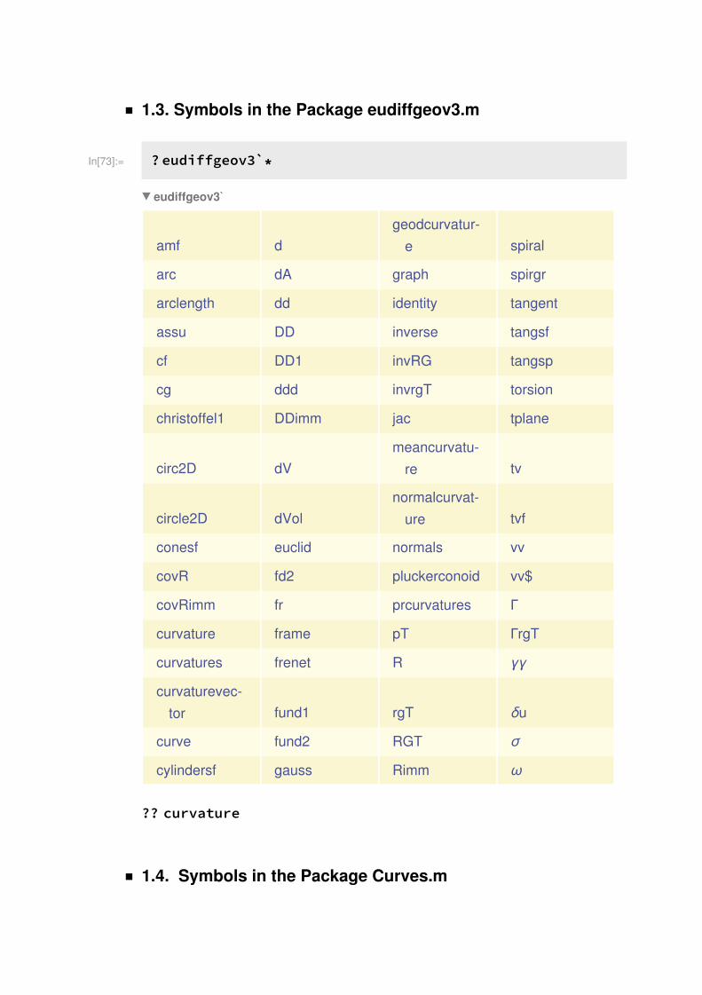
◼ 1.3. Symbols in the Package eudiffgeov3.m
In[73]:= ?eudiffgeov3`*
eudiffgeov3`
amf d
geodcurvatur-
e spiral
arc dA graph spirgr
arclength dd identity tangent
assu DD inverse tangsf
cf DD1 invRG tangsp
cg ddd invrgT torsion
christoffel1 DDimm jac tplane
circ2D dV
meancurvatu-
re tv
circle2D dVol
normalcurvat-
ure tvf
conesf euclid normals vv
covR fd2 pluckerconoid vv$
covRimm fr prcurvatures Γ
curvature frame pT ΓrgT
curvatures frenet R γγ
curvaturevec-
tor fund1 rgT δu
curve fund2 RGT σ
cylindersf gauss Rimm ω
?? curvature
◼ 1.4. Symbols in the Package Curves.m
◼ 1.5. Symbols in the Global Context
2. Regular Curves. Examples in the Euclidean
Plane
In this Section we develop basic concepts of the differential geometry of
curves; as example we consider curves in the Euclidean plane.
◼ 2.1. Definitions
◼ 2.1.1. Regular Curves. Tangents
◼ 2.1.2. Arc Length
◼ 2.2. Curvature. Graphs. Spirals
◼ 2.3. Frenet Formulas for Plane Curves
◼ 2.3.1. The Fundamental Theorem
◼ 2.3.2. Examples
◼ 2.3.3. Curves Represented with an Arbitrary Parameter
3. Curves in the Euclidean Space
Now we consider curves in the three-dimensional Euclidean space. Our
aim is to describe the basic invariants of the
curves, the curvature and the torsion, and create Mathematica Modules to
calculate them.
◼ 3.1. Settings. The General Curve: curve3D
◼ 3.2. Frenet Formulas for Space Curves
◼ 3.3. Applications
◼ 3.3.1. Plane Curves as Special Space Curves
◼ 3.3.2. Helices and 1-Parameter Subgroups of the Euclidean Group
◼ 3.3.3. Very Flat Curves
4. Osculating Circle and Osculating Sphere
Using the Frenet frame of a curve in the n-dimensional Euclidean space we
construct Modules to calculate the osculating circle and the osculating
sphere of the curve.
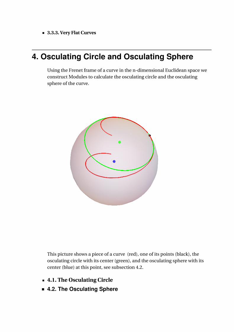
This picture shows a piece of a curve (red), one of its points (black), the
osculating circle with its center (green), and the osculating sphere with its
center (blue) at this point, see subsection 4.2.
◼ 4.1. The Osculating Circle
◼ 4.2. The Osculating Sphere
◼ 4.3. Examples
In this Subsection we consider three examples. Use the definitions of space
curves inA. Gray’s package Curves3D.m, see also Subsection6.1.
◼ 4.3.1. genhelix
◼ 4.3.2. ast3d
◼ 4.3.3. sinn
5. Curves of Constant Curvatures and 1-
Parameter Motion Groups
Applying the built-in Mathematica function MatrixExp the curves of
constant curvatures are treated here as orbits of 1-parameter motion
groups. In particular it is shown that the orbits of maximal rank in the four-
dimensional space are the isogonal trajectories of the family of generating
circles of tori.
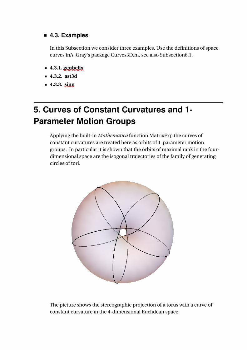
The picture shows the stereographic projection of a torus with a curve of
constant curvature in the 4-dimensional Euclidean space.
◼ 5.1. Screw Motions in the Euclidean 3-Space
◼ 5.2. Curves of Constant Curvatures in the Euclidean 4-Space
◼ 5.3. The Shape of the Orbits of Rank 4
◼ 5.4. Isogonality
◼ 5.5. Higher Dimensions
6. Examples. DSolve. NDSolve
◼ 6.1. Alfred Gray’s Space Curves
In this subsection we plot some curves and calculate their invariants. The
user may continue considering other curves of Gray’s list or creating new
curves.
◼ 6.1.1. Initialization
◼ 6.1.2. Astroid in 3D
◼ 6.1.3. Elliptical Helix
◼ 6.1.4. The Twicubic
◼ 6.1.5. Viviani Curves
◼ 6.1.6. Power Functions
◼ 6.2. Solution of the Frenet Equations
In this experimental Section we try to use the Mathematica built-in
programs Dsolve and NDSolve to obtain solutions of the Frenet equations
with given curvature function.
◼ 6.2.1. DSolve
◼ 6.2.2. NDSolve
◼ 6.2.3. Further Examples Using NDSolve
References

Homepage


