
IZA DP No. 294
Estimating the Effect of UnemploymentInsurance Compensation on the Labor MarketHistories of Displaced WorkersStepán Jurajda
DI
SC
US
SI
ON
PA
PE
R S
ER
IE
S
Forschungsinstitutzur Zukunft der ArbeitInstitute for the Studyof Labor
May 2001

���������������� ���������������������� ��������������������������������������������� ���������
���
�� � �!���"��������������������� ��������� �
��
Discussion Paper No. 294 May 2001
IZA
P.O. Box 7240 D-53072 Bonn
Germany
Tel.: +49-228-3894-0 Fax: +49-228-3894-210
Email: [email protected]
This Discussion Paper is issued within the framework of IZA’s research area ������������������ ��������������� �Any opinions expressed here are those of the author(s) and not those of the institute. Research disseminated by IZA may include views on policy, but the institute itself takes no institutional policy positions. The Institute for the Study of Labor (IZA) in Bonn is a local and virtual international research center and a place of communication between science, politics and business. IZA is an independent, nonprofit limited liability company (Gesellschaft mit beschränkter Haftung) supported by the Deutsche Post AG. The center is associated with the University of Bonn and offers a stimulating research environment through its research networks, research support, and visitors and doctoral programs. IZA engages in (i) original and internationally competitive research in all fields of labor economics, (ii) development of policy concepts, and (iii) dissemination of research results and concepts to the interested public. The current research program deals with (1) mobility and flexibility of labor markets, (2) internationalization of labor markets and European integration, (3) the welfare state and labor markets, (4) labor markets in transition, (5) the future of work, (6) project evaluation and (7) general labor economics. IZA Discussion Papers often represent preliminary work and are circulated to encourage discussion. Citation of such a paper should account for its provisional character.

IZA Discussion Paper No. 294 May 2001
#$%&'#�&
���������������� ���������������������� �������������������������������������
�������� ���������∗ In this paper, U.S. data on labor market histories of displaced workers are used to quantify the effect of Unemployment Insurance Compensation (UIC) on both unemployment and employment durations. This results in the first available assessment of the effect that UIC has on the fraction of time spent employed. The estimation procedure simultaneously allows for unobserved heterogeneity, defective risks and sample selection into future spells, and uses alternative assumptions about agents’ knowledge of the UIC eligibility rules. Being entitled to UIC shortens workers’ employment durations. This negative effect on the fraction of time spent employed could be offset by suspending an extended benefits program in order to shorten unemployment durations. JEL Classification: C41, J63, J65 Keywords: Employment durations; unemployment insurance; unmeasured heterogeneity;
defective risks; sample selection Št ��������� CERGE-EI POB 882 Politickych veznu 7 Prague 1, 111 2 1 Czech Republic Tel.: +420-2-24005 139 Fax.:+420-2-242 11374 E-mail: [email protected]
∗ A joint workplace of the Center for Economic Research and Graduate Education, Charles University, and the Economics Institute of the Academy of Science of the Czech Republic.

1. Introduction
While there have been numerous studies estimating the effect of unemployment insurance compen-
sation (UIC) on duration of unemployment, there has been no empirical work analyzing the effect
of UIC on employment durations in the United States.1 This gap in the literature is somewhat
surprising since there are at least two theoretical arguments for why we would expect UIC to affect
employment durations. First, the implicit contract literature suggests that unemployment insurance
makes layoffs more likely (e.g., Feldstein, 1976; Baily, 1977). Second, job search models suggest that
workers with generous UI coverage will search less intensively while unemployed. As we discuss in
section 3, one can show that the optimal Þrm response to this behavior, in the presence of demand
ßuctuations and Þrm speciÞc human capital, is for the Þrm to lay off workers with high levels of UI
entitlement and recall workers as they approach exhaustion of their beneÞts.
Hence, generous UIC may not only prolong unemployment (e.g., Mortensen, 1977), but also
shorten employment duration, reinforcing the combined negative effect of UIC on the fraction of
time spent employed. To see this in a simple setting, consider the steady state probability of being
employed, Pe, which can be written as
Pe =Ee
Ee +Eu, (1)
where Ee is the expected duration of employment and Eu denotes the expected duration of unem-
ployment, both being functions of the level of UIC. It follows that
∂Pe∂UIC
= [Ee +Eu]−2
·∂Ee∂UIC
Eu − ∂Eu∂UIC
Ee
¸.
Evaluating unemployment insurance based on only the existing (positive) estimates of its effect on
unemployment duration³∂Eu∂UIC
´may therefore result in underestimating the total impact of UIC.
1The only studies looking at employment durations we are aware of are Baker and Rea (1998) and ChristoÞdesand McKenna (1996). Both analyze the effect of Canadian UI eligibility requirements. There is extensive researchin the U.S. using cross-sectional data to analyze the layoff effect of unemployment insurance taxes. We discuss thiswork in section 2; analyzing this issue, however, is beyond the scope of the present paper. As we explain below, theamount of potential UIC a worker can expect to receive varies over the duration of individual employment spells;hence, the need to use duration data.
2

In this paper we therefore quantify the effect of UIC on both unemployment inßow and outßow
using a micro data set on labor market histories of U.S. workers. As a result, we obtain the Þrst
available assessment of the effect UIC has on the fraction of time spent employed. Relaxing the
steady state assumption used above, we quantify the overall effect of UIC by simulating the process
of Þnding and losing jobs for all individuals in our data under different levels of UIC.
The lack of research on the UIC employment duration effect is likely caused by the fact that
large micro data sets on employment durations and UI compensation are scarce. We use a data
set which consists of a dislocated workers� survey, augmented with information on the amount
of UI compensation individuals can expect to receive if they are laid off or quit. Unemployment
compensation provisions, including the trigger dates of various extended beneÞt programs, are coded
for over Þve years for seven states. The resulting multiple-spell, event-history data set is unusually
rich in terms of the variation of entitlement and beneÞt levels.
The use of hazard models in analyzing duration data has become widespread, and accounting
for unobserved heterogeneity is now a standard part of hazard estimation sensitivity analysis. The
estimation procedure used here allows for the effects of unobserved heterogeneity in a number
of ways and controls for sample selection into multiple spells, a potentially important issue in
the estimation of duration models: Using multiple-spell data on employment and unemployment
durations provides greater variation and improves identiÞcation of the unobserved heterogeneity
distribution (Heckman and Singer, 1984). The use of this type of data, however, also raises the
possibility of selection bias: i.e., the workers who have multiple employment spells may be a non-
random sample. To control for this problem, we estimate employment and unemployment durations
jointly while allowing the unobserved heterogeneity to be correlated across these spells.2
The estimation of employment duration effects of UIC also requires a separate focus on different
2For a similar approach and for a discussion of dynamic sample selection in multiple-state, multiple-spell data, seeHam and Lalonde (1996). They Þnd important sample-selection bias when estimating the effect of classroom trainingon employment histories of disadvantaged women. In the present study, the level and availability of UIC dependson workers� employment histories. To the extent that employment histories are driven by unobservables, this mayintroduce dependence between UIC and unobservable heterogeneity, biasing the estimation of the UIC effects.
3
ways of exiting an employment spell. A worker who quits will generally not be entitled to UI
compensation. In the presence of a positive layoff probability, delaying a quit to non-employment
will provide the worker with a chance of getting laid off and obtaining UI coverage. Thus, one may
expect the opposite entitlement effects when comparing layoff and quit decisions, which motivates
a separate analysis of quits and layoffs in a competing risk duration model. The richest estimated
model is therefore a multiple-spell, multiple-state competing risk duration model with unobserved
heterogeneity. Finally, the estimated unobserved heterogeneity models naturally extend to account
for the possibility of defective risks (zero probability of a quit for a fraction of the sample).
The theory modeling worker (Þrm) response to UIC is forward-looking: it evaluates future
streams of income (proÞt). The nature of the UIC system, however, makes it hard to predict
future level and availability of UIC, which depend on individual labor market histories as well as
on the evolution of the labor market. Any attempt to evaluate the effects of UIC on economic
outcomes therefore has to rely on arbitrary assumptions about how agents form expectations of
the available UI compensation.3 In this paper, we examine the robustness of the empirical results
with respect to different assumptions about how Þrms and workers account for UIC rules when
determining eligibility for future UI claims. This issue has not been addressed previously. The
type of assumption one makes in the estimation signiÞcantly affects the levels of the explanatory
variable of interest�UI entitlement. In the empirical analysis we therefore compare results based on
the assumption that future UI eligibility is ignored to results based on the assumption that future
UI eligibility is taken into account.
The empirical results suggest that being entitled to UI compensation signiÞcantly increases the
layoff hazard (deÞned as the probability of getting laid off in a given week conditional on being
employed up to that week). In contrast to theoretical prediction, however, neither the length of
3For example, the availability of extended UI beneÞts depends on the evolution of the state (insured) unemploymentrate. Rogers (1998) estimates the UIC effect on unemployment outßow (hazard) and examines the robustness of theestimates with respect to different assumptions about agents� expectations. Her results imply that workers havesigniÞcant, although not perfect, foresight about changes in UI provisions.
4

potential UI entitlement nor the dollar amount of UI beneÞts, conditional on being positive, affect
the layoff hazard. The quit hazard is not affected by any of the UI system parameters. Findings
on the UI effect on unemployment outßow are in accord with the existing literature.
To measure the magnitude of the estimated UIC effects, we study the fraction of time (sampling
frame) spent in employment under various policy experiments. This exercise suggests that the
positive UIC layoff effect, which shortens employment durations and lowers the fraction of time
spent employed, could (roughly) be offset by shortening of unemployment durations corresponding
to suspending an extended beneÞts program. (See Section 4 for deÞnitions of extended beneÞts
programs.)
The paper proceeds as follows. Section 2 discusses previous work and Section 3 models Þrm
employment decisions. The data set is described in Section 4. Section 5 presents the econometric
approach together with the empirical results. Section 6 concludes.
2. Previous Work
There is a large volume of research, based on the optimal job search theory (Mortensen, 1977),
analyzing the effect of UIC on the duration of unemployment. For a survey of the search-theoretic
empirical literature, see Devine and Kiefer (1991). The strand of economic literature focusing on
(temporary) layoffs and unemployment insurance, however, is smaller in volume. It starts with
the analyses of implicit contract models by Feldstein (1976) and Baily (1977). In these models,
Þrms facing competitive labor markets have to offer employment contracts which provide workers
with a market-determined level of expected utility. While Feldstein�s 1976 model focuses on the
role of imperfect experience rating of Þrms in the presence of product demand ßuctuations,4 Baily
(1977) shows that increases in the level of UIC cause Þrms to increase layoffs: Since workers with
UI coverage are better protected against prolonged spells of unemployment, the layoff probability
4The U.S. system of levying unemployment insurance tax based on an employer�s unemployment experience iscalled experience rating.
5
becomes an increasing function of UIC.5
Implicit contract models assume workers� utility level is exogenous and endogenize the level
of wages. On the other hand, models focusing on the adjustment cost aspect of UI taxes6 (e.g.,
Card and Levine, 1992) take wages as exogenous. Firms are at least partially responsible for UI
beneÞts paid to their former employees. A typical adjustment cost model would therefore imply that
more generous UI coverage leads to lower risks of layoff, contrary to predictions of implicit contract
models. Anderson and Meyer (1994) extend the adjustment cost model to include the compensation
package concept of implicit contract models. While all models predict a negative relation between
the degree of experience rating and layoffs, their analysis allows for different effects of UIC.
The theoretical work discussed above has motivated a number of empirical studies focusing on
experience rating. Typically, these studies use CPS cross-sectional data sets (e.g., Topel, 1983; Card
and Levine, 1992) and suggest that the unemployment inßow effect of UI is potentially quite large
because of imperfect experience rating. Anderson and Meyer (1994) analyze cross-sectional data
sets based on the Continuous Wage and BeneÞt History (CWBH) survey to quantify the effects
of experience rating and the level of potential UI coverage on the incidence of layoffs. While they
conÞrm previous Þndings of large experience-rating effects, they obtain conßicting estimates of the
effect of potential UI coverage.
Baker and Rea (1993) and ChristoÞdes and McKenna (1996) analyze the effect of Canadian UI
eligibility rules to identify spikes in the employment hazard (i.e., the hazard of leaving employment)
in the Þrst week of eligibility. Canadian eligibility rules depend on local economic conditions, but
Baker and Rea (1993) are able to untangle this dependency by using a unique change in the eligibility
formula orthogonal to changes in the economic environment. Their results indicate a signiÞcant
increase in the employment hazard in the week in which individuals qualify for UI compensation.
5The implicit contract analysis is generalized by Burdett and Hool (1983), who incorporate the optimal contractdetermination into a bargaining problem of Þrms and workers, and by Haltiwanger (1984), who analyzes a multiperiodcontract model allowing for the interaction of stock adjustment and factor utilization decisions.
6UI taxes make employment adjustment costly because of experience rating.
6
Other than including three dummy variables capturing UI eligibility,7 they do not control for the
level of available UI compensation. In particular, they do not control for the dollar amount of UI
beneÞts available and for changes in the maximum amount of UI entitlement.
This paper extends the existing literature by analyzing the effect of UI on employment durations
in the U.S., using different, rich sources of variation in UI compensation8 and considering quits and
layoffs separately.
3. A Dynamic Model of Layoffs9
Consider a dynamic decision problem of a price-taking, proÞt-maximizing Þrm deciding on the
employment status of a Þxed roster of workers.10 Wages are Þxed at w and the Þrm faces demand
ßuctuations assumed to take the form of i.i.d. draws from a Þrm-speciÞc distribution of marginal
revenue product M of its workers. Workers differ only in their UI entitlement, measured in length
of available beneÞts collection. An employed worker brings the Þrm a per-period proÞt of M− w.A laid off worker collects UIC until beneÞts lapse. He may either be recalled or accept a position
with a different employer. If the Þrm Þnds it proÞtable to replace a worker lost to another employer
with a new worker, it incurs training costs. The key assumption is that a laid off worker follows
the optimal job search strategy (Mortensen, 1977), which is known to the Þrm.11
Based on these assumptions and appealing to Bellman�s principle of optimality, one can deÞne
the Þrm�s proÞt value function from having a worker employed. Since the function is monotonically
increasing in the value of marginal revenue product M , there is an optimal layoff stopping rule m,
7The Þrst one equals one in the week when a given worker becomes eligible. The second indicates that the worker�sentitlement is between the minimum and maximum value. The third dummy variable equals one when the workerhas attained the maximum potential entitlement.
8Anderson and Meyer (1994) use state variation in entitlement and beneÞts coming from the high quarter wageand base period earnings, which together with the state level of the maximum beneÞt amount are used to determineregular beneÞt amount and duration.
9This section is a simpliÞed non-technical summary of a dynamic optimization problem analyzed in Jurajda (2000).10A similar assumption of a Þxed roster of workers was used in most previous studies, e.g. Feldstein (1976) and
Card and Levine (1992), to narrow the model�s focus to temporary layoffs. The workers are attached to the Þrmthrough Þrm-speciÞc training.11The important maintained assumption is that workers do not take the optimal recall strategy of Þrms into account
when optimizing their search behavior.
7
such that the Þrm decides to keep the worker at all M ≥ m and to lay off otherwise.12 Similarly,
one can write a proÞt value function from having a worker on layoff. The optimal layoff stopping
value of marginal revenue product m is then implicitly deÞned by the equality of the proÞt value
functions in the two states, employment and unemployment, evaluated at the optimal stopping rule.
That is, at M = m, the Þrm is indifferent between laying off or retaining a worker.
This implicit deÞnition can be used to study properties of the optimal decision rule m. A
standard result from the job search literature is that the probability of a worker on layoff Þnding a
job with a Þrm is a decreasing function of the length of the remaining UI entitlement period. Hence,
assuming that the Þrm takes workers� search strategies into account, laying off a worker with a high
value of potential UI entitlement is less costly for the Þrm since such a worker will be less likely to
Þnd a new acceptable job with an alternative employer. One can therefore show that the per-period
layoff probability increases with the level of UIC entitlement, motivating layoff hazard estimation
of the UIC effect much the way job search models motivate estimation of (new job) unemployment
hazards.13
A worker who quits will generally not be entitled to UI compensation, and so one might expect
opposite entitlement effects when comparing layoff and quit decisions: Clearly, there will be no
effect of UI compensation on job-to-job quits. Quits to non-employment are present in the job
matching models (e.g., Jovanovic 1979). If there is a positive probability of getting laid off, it
could pay off for a worker contemplating a quit to non-employment to stay employed one more
period, since by doing so he could get laid off and be qualiÞed for UI coverage. The higher the
available UI compensation, the stronger the incentive to wait for (or induce) layoff. Workers with
high entitlement can therefore be expected to be less likely to quit.
12The value function consists of the per-period proÞt rate M −w and the discounted future proÞts in three possiblestates, weighted by their respective probability: First, if there is no change in M , the Þrm faces a similar optimizationproblem next period. Second, the Þrm evaluates the expected proÞts resulting from employing a worker at a newlyarriving value of M above the layoff threshold m. Third, when a below-the-threshold value of M arrives, the workeris laid off and the Þrm expects to receive the proÞt value function from having a worker unemployed.13Similarly, one can show that it is optimal for the Þrm to recall workers with higher probability as they approach
exhaustion of their beneÞts, providing motivation for recall hazard estimation.
8
4. Data Description
The data employed in this paper come from the Trade Adjustment Assistance (TAA) Survey.
Implemented in 1974, the TAA program was intended to compensate workers harmed by market
ßuctuations resulting from a rise in imports.14 The data was collected from retrospective interviews
with individuals who became unemployed in the mid 1970s. This information was merged with UI
claims records. The data comes from seven states15 and covers the period up to 1979. The TAA
recipients were entitled to extensions of the regular UI entitlement of up to 52 weeks. Also, their
replacement ratio (i.e. the ratio of UI beneÞts to wages on the last job) was set at 70% as opposed
to the 50% typical of regular UI. Both regular UI recipients and TAA recipients are included in the
sample.16 The combination of TAA and UI recipients leads to a rich variation in UI entitlement and
beneÞts. The other attractive feature of this sample is that it covers a period with many dramatic
changes in UI entitlement, caused by various extended coverage programs being triggered on and
off. Further, with the exception of the Survey of Income and Program Participation (SIPP), it
appears to be the only U.S. data set on employment durations.
During the sample period there were two types of extended coverage programs in effect: the
Extended BeneÞts program and the Federal Supplemental BeneÞts program. These programs trigger
on and off based on state and national insured unemployment rates. The State-federal Extended
BeneÞts program triggers both at state and national levels and adds up to 13 weeks of UI beneÞts
(50% beyond the state potential duration). The Federal Supplemental BeneÞts program extended
the previous entitlement by up to 26 additional weeks of UI compensation. It was enacted at the
national level and the number of extra weeks of UI differed both across states and over time.17 The
two programs could therefore change the typical 26 weeks of regular UI entitlement by as much as
39 weeks. Most of the empirical leverage necessary for the identiÞcation of the entitlement effect14The program was amended several times and is still active.15California, Indiana, Massachusetts, New York, Ohio, Pennsylvania and Virginia.16For a thorough description of the data and for information about the TAA program, see Corson and Nicholson
(1981).17A brief description of these programs can be found in Jurajda (1997).
9

comes from these programs, as well as from the combination of UI and TAA recipients.
Note that potential entitlement can also be quite low in some cases. Consider a worker who is
recalled or Þnds a new job only a few weeks prior to exhausting UI beneÞts. Before he accumulates
enough earnings to be eligible for the full UI entitlement, the worker faces the possibility of layoff
with a low value of entitlement left from the previous spell of unemployment. Hence, the existence
of the UI beneÞt year is another source of variation in potential entitlement. The UI beneÞt year
starts when a UI claim is Þled, at which moment the initial entitlement is determined based on the
eligibility requirements. If a worker becomes employed after a few weeks of unemployment, a large
amount of entitlement remains available for the duration of the UI beneÞt year. However, potential
entitlement for those workers with only a few weeks left in their UI beneÞt year can be less than the
remaining (non-collected) part of their initial entitlement. Hence, potential entitlement can also
vary with time left in a UI beneÞt year.
From the initial sample of 1,501 men and women we work with the subsample of 953 men. We
drop 102 cases in which the initial unemployment spell was in fact a period of reduced hours and
14 workers who do not start an employment spell during the sample frame.18 Finally, inconsistent
and missing data records were deleted, yielding a sample of 808 men, of which 62% collect TAA
in the initial unemployment spell. The data is recorded for a period of about 3.5 years for each
individual and includes no simultaneous job holdings. The initial spell of unemployment is followed
by an employment spell for all 808 workers. Approximately 50% of the Þrst employment spells are
censored and about half of the subsequent unemployment spells end in another employment spell.
Moreover, about 10% of workers experience three employment spells within the sample frame; these
individuals have lower than average durations of both unemployment and employment.19 The ex-
istence of this group of workers with short employment and unemployment durations suggests the
18These 14 workers report being out of the labor force at the time of the interview. This raises a sample selectionissue as they may have been active job seekers when they Þrst lost their job. However, given the small number ofsuch workers, this issue is not explored in the empirical analysis.19Only about 10% of those who enter second and third jobs are construction workers.
10
possibility of substantial unobserved heterogeneity correlated across spells and states and affecting
the selection into multiple spells. Such dynamic sample selection (on unobservables) may correlate
unobservable heterogeneity with the UIC variables because the UI eligibility rules make the avail-
able UI compensation depend on workers� labor market histories. This issue (of potential bias in
estimating the UIC effects) will be explored in the empirical analysis.
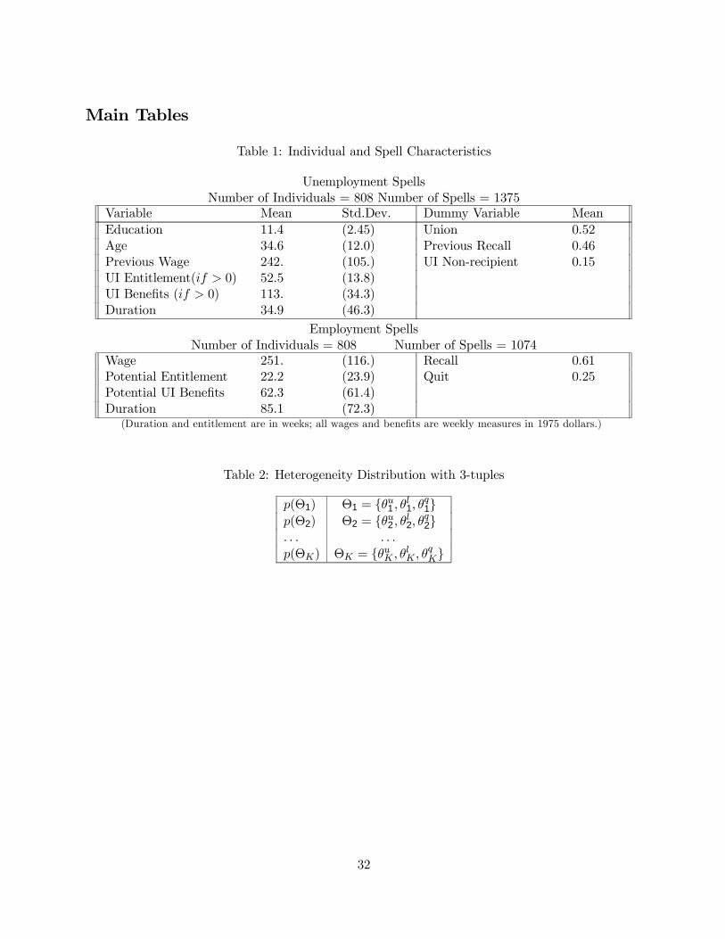
Table 1 shows the data means at the Þrst week of spells for all 808 men. The averages for
unemployment spell beneÞts and entitlement in the current UI claim are taken over UI recipients
only. The non-recipients consist primarily of people who have quit their previous jobs. The low
average values of UI beneÞts and entitlement in the Þrst week of employment spells come from the
fact that, at the beginning of a spell, individuals are sometimes not eligible for UI compensation.
The reported standard deviations of the UI variables reßect only the cross-sectional variation in the
Þrst week of each spell. Additional time variation used in the estimation comes mostly from the
extended coverage programs, which change the amount of available compensation even for spells in
progress.
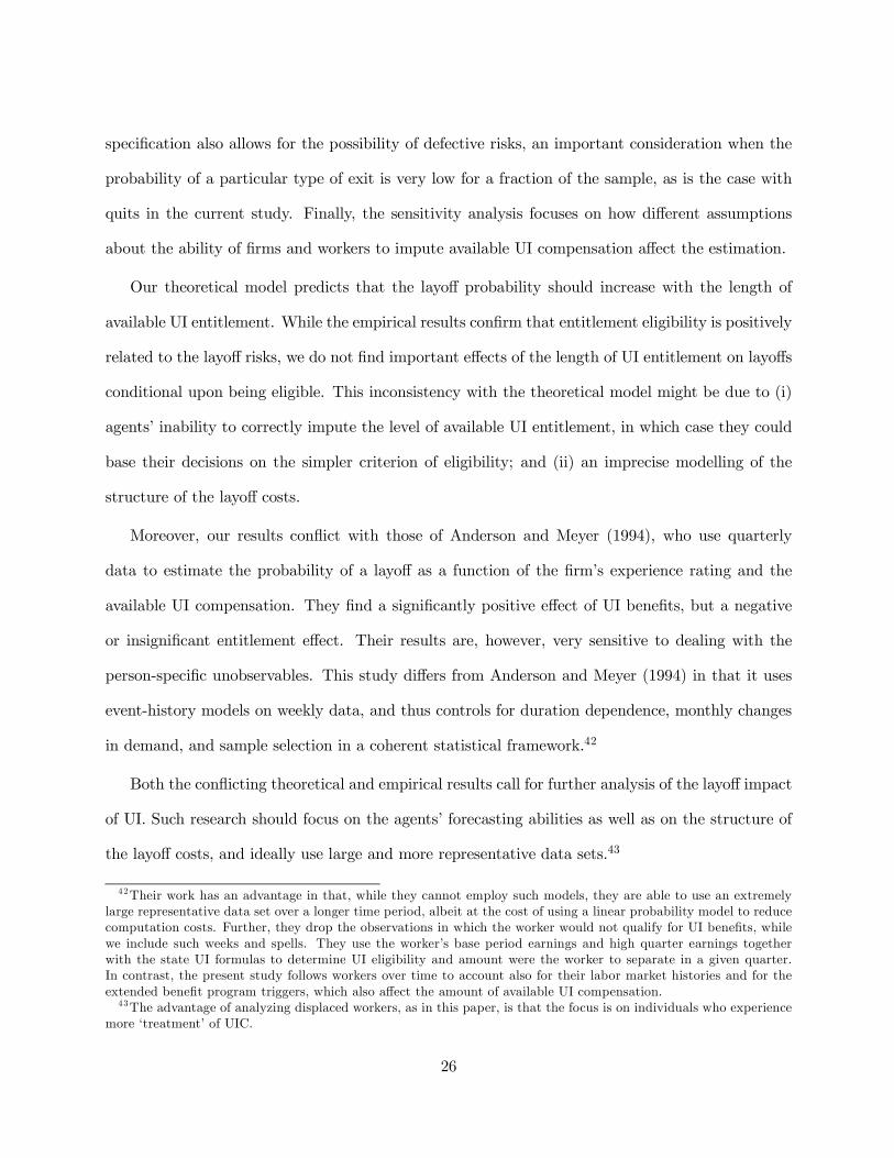
The simplest approximation to the underlying hazard functions which ignores both observed
and unobserved differences in the population is provided by the Kaplan-Meier empirical hazards. A
basic set of empirical hazards is presented in Appendix 6, which contains the overall unemployment
empirical hazard with one standard deviation bounds. It also presents empirical hazards for the
employment spells (overall and competing risks), and reveals differences between layoffs and quits
(the layoff hazard is larger than quit hazard in the Þrst 40 weeks of duration) as well as spikes
at approximately one year of duration, reßecting perhaps the end of a probation period or recall
bias.20
The data set contains information on the level of initial entitlement and beneÞts only for the
Þrst unemployment spell. We impute both (i) the potential entitlement for the employment spells
20Recall bias occurs when individuals who do not recall the exact duration of their employment spell report ap-proximate duration rounded to the closest six-month period, for example.
11
and (ii) the actual entitlement levels for the second and third unemployment spell from the state
speciÞc UI laws and the individual data. To impute the UI compensation, we use the level of initial
entitlement in the Þrst unemployment spell and follow each individual over time, determining the
level of entitlement in each week based on the individual�s employment history, information on the
reason for job separation (i.e. quit as opposed to layoff21), UI eligibility requirements, and the
effective trigger dates of extended beneÞts programs. In the imputation procedure we assume that
workers Þle UI claims whenever they are entitled to do so. When determining eligibility we also
assume that wages do not change on the job (only accepted wages are reported).22
Using predicted values of UI entitlement instead of actual ones is a potential drawback of the
data. Note, however, that workers or Þrms contemplating a transition out of employment will have
to use their own prediction of potential entitlement based on a similar information set. Thus, we
would argue that our prediction of the potential UI compensation should not signiÞcantly affect the
results, at least in the employment spells.
One important question arising when imputing potential entitlement values is whether workers
and Þrms are able to determine the UI eligibility for future UI claims. For example, is a recently
recalled worker with only 10 weeks of entitlement left from his spell of unemployment able to
predict that if he were laid off at that time, he would (after exhausting the remaining 10 weeks of
entitlement) become eligible for another UI claim? If so, then the value of potential entitlement
should equal the sum of the remaining UI compensation from the existing UI claim, plus the initial
UI entitlement a newly eligible worker would obtain at the beginning of a new UI claim. This
assumption on potential entitlement seems reasonable since all of the workers in the sample went
through the process of Þling the initial UI claim at the beginning of the sample frame and, therefore,
should have at least some understanding of what the UI eligibility requirements are. Similarly, Þrms
can be assumed to know the UI rules as they face layoff decisions on a regular basis. Assuming that
21There were only a few cases of an individual being Þred for cause, and they are omitted in the empirical analysis.22The information sources used in imputing UI compensation are listed in Jurajda (1997).
12

UI eligibility rules are well known, a recently recalled worker who becomes eligible for a new UI claim
during his current UI claim will have higher potential UI entitlement than a worker who has been
on a job for over one year. Taking future repeated UI claims into account therefore breaks the usual
positive relationship between the level of potential UI entitlement and job duration. On the other
hand, it may be that Þrms and especially workers are somewhat myopic in measuring potential UI
entitlement. In the estimation we therefore allow for alternative assumptions on whether individuals
account for UI eligibility rules when determining future entitlement.
5. Estimation and Results
A typical job search model derives the per period escape rate out of unemployment as a function of
the remaining UIC. Job search models therefore naturally motivate the estimation of unemployment
hazard functions, which parametrize the probability of leaving unemployment at each time period.
Similarly, estimation of the employment quit process has been motivated by on-the-job search
models (e.g., Burdett 1978). Finally, the model of layoff decisions discussed in Section 3 derives
the optimal per period layoff rate as a function of the UIC and motivates estimation of a layoff
hazard function. The reduced-form hazard model used here therefore estimates the conditional
probability of (i) Þnding a job while unemployed or (ii) losing a job while employed. The resulting
estimates for employment or unemployment durations can be interpreted as approximations to
the comparative statics implied by a corresponding model of job separations or job search. The
theoretical considerations presented in Section 3 also point to a differential effect of UI on quits and
layoffs and lead to a competing risks estimation of employment hazard functions.23
5.1. Econometric Model
The duration model builds upon the concept of a hazard function, which is deÞned as the probability
of leaving a given state at duration t conditional upon staying there up to that point. Using this
23 In the unemployment hazard we do not differentiate between recalls and new job Þndings since this issue hasbeen analyzed extensively in the existing literature (e.g., Katz and Meyer, 1990).
13
deÞnition one can build a likelihood function for the observed durations and estimate it using
standard methods. However, it is well known that in the presence of unobserved person speciÞc
characteristics affecting the probability of exit, all of the estimated coefficients will be biased. To
control for unobserved factors, we follow the ßexible approach of Heckman and Singer (1984). The
strategy is to approximate any underlying distribution function of unobservables by estimating a
discrete mixing distribution p(θ) of an unobserved heterogeneity term θ as a part of the optimization
problem.
More speciÞcally, let λj(t, xt|θjk) be the conditional probability (hazard) of leaving a given state
at time (duration) t for someone with person speciÞc characteristics xt, conditional upon this person
having the unobserved factor θjk, k=1, 2, ...,Njθ . The j subscript stands for the different ways of
leaving a given state and serves, therefore, as a state subscript as well. For example one can leave
employment through a quit or through a layoff, in which case j ∈ {q, l}. This is often referred to
as a competing risk model. In what follows, we work in discrete time with weekly hazards in logit
speciÞcation:
λj(t, xt|θjk) =1
1 + e−hj(t,xt|θjk
),(1)
where
hj(t, xt|θjk) = rj(et,αj) + β0jzt + gj(t, γj) + θjk. (2)
Here, x0t = (et, z0t), rj(et,αj) denotes a function of remaining entitlement et, the vector zt includes
levels of beneÞts, wages, demographics and time changing demand measures.24 Finally, gj(t, γj) is
a function capturing the duration dependence.
To give an example of how the sample likelihood is evaluated in a competing risks speciÞcation
with layoff and quit hazards, assume away any complications arising from the presence of unobserved
heterogeneity. Under the assumption that layoff notes arrive in the morning mail, before quit
decisions are contemplated, the unconditional probability of someone leaving employment through
24 In order to streamline notation, we do not use individual i subscript in any of the formulas.
14
a layoff at duration t is
Lle(t) = λl(t, xt)Se(t− 1), where Se(t− 1) =t−1Yv=1
[1− λq(v, xv)][1− λl(v, xv)], (3)
and where λq and λl denote the quit and layoff hazards respectively. Se(t− 1) gives the probabilityof a given spell lasting at least t − 1 periods. A likelihood contribution of a quit at duration t isdeÞned similarly:
Lqe(t) = λq(t, xt)(1− λl(t, xt))Se(t− 1). (4)
For an employment spell which is still in progress at the end of our sampling frame, at time T, one
enters the employment survival probability Se(T ). The sample likelihood then equals the product
of individual likelihood contributions.
Next, allow for multiple employment and unemployment spells and introduce unobserved hetero-
geneity. The primary tool for dealing with unobserved factors is a heterogeneity distribution which
uses N-tuples of unobserved factors (McCall 1996), where N is the number of hazard functions
to be estimated. The reemployment and job exit processes create correlation between unobserved
characteristics in different types of spells. Thus, the competing risks employment hazards, the
overall unemployment hazard and the unobserved heterogeneity distribution are estimated jointly,
allowing for a full correlation structure of the unobservables. This general type of heterogeneity is
parametrized using the 3-tuple distribution described in Table 2, where u, l and q denote overall
unemployment hazard, layoff and quit employment hazards, respectively. K denotes the number of
estimated points of support of the mixing distribution.
To see an example of how the likelihood is formed, consider a worker leaving the Þrst unem-
ployment spell after t weeks , then getting laid off after s − t weeks on a job and staying in the
second unemployment spell till the date of the interview, say at T − s weeks into the last spell. Hislikelihood contribution becomes
Lu,l,u(t, s, T ) =KXk=1
p(Θk)Lu(t|θuk)Lle(s|θqk, θlk)Su(T |θuk), (5)
15

where Θk ≡ (θqk, θlk, θuk), p(Θk) is the probability of having the unobserved components Θk, and
Lle(s|θlk, θqm) = λl(s, xt|θlk)s−1Yv=1
[1− λl(v, xv|θlk)][1− λq(v, xv|θqm)]. (6)
Finally, the unemployment spell likelihood contributions in Equation 5 are deÞned analogously:
Lu(t|θuk) = λu(t, xt|θuk)t−1Yv=1
[1− λu(v, xv|θuk)] and Su(T |θuk) =TY
v=s+1
[1− λu(v, xv|θuk)]. (7)
One can compute individual contributions to the sample likelihood for other labor market histo-
ries in a similar way. The number of points of support of the distribution of unobservables (Nuθ , N
qθ
and N lθ) is assumed to be Þnite and is determined from the sample likelihood. Note the assumption
of θu, θq and θl staying the same across multiple unemployment and employment spells respectively.
Detailed estimation strategy issues are discussed below.
5.2. Employment Hazard Estimates
We start by estimating the employment hazard functions with no unobserved heterogeneity.25 In
terms of the notation introduced in Section 5.1, θk= θ ∀k. Table 3 contains the estimates for thecompeting risks employment hazard functions based on assuming Þrms and workers do not take
eligibility for future UI claims into account. Let us Þrst discuss the layoff hazard estimates. In
column (1) we control for the potential UI compensation by including a dummy variable equal to
one in each week when a given worker would be entitled for UI in the case of a layoff. We also
control for the potential dollar amount of weekly UI beneÞts. Being entitled to UI compensation
signiÞcantly raises the layoff hazard. The negative estimate of the potential beneÞts coefficient
contradicts the economic intuition of our model but is not precisely estimated. Higher beneÞts lead
to lower risks of layoff in the adjustment cost models (e.g., Card and Levine, 1992).25The employment hazard empirical speciÞcations capture the effect of explanatory variables on the length of
an employment spell, which does not correspond to the cummulated job duration (seniority) for recalled workers.Our focus is on the effect of UI on job separations, and not on the issue of seniority. The amount of potential UIcompensation -which is computed for each individual at each point in time- is based on the length of employmentspells and earnings in the base period and does not depend on the duration of a speciÞc worker-Þrm employmentrelationship.
16

Next, we allow for effects of the length of available entitlement, conditional on the worker being
eligible. SpeciÞcally, we add a step function in the value of entitlement. The base case are those with
more than 52 weeks of available UI compensation.26 The table also reports the fraction of weekly
observations covered by each of the entitlement steps. Column (2) lists the estimated coefficients
which indicate that, conditional on eligibility, the amount of entitlement plays no role in the Þrm�s
layoff decisions as the steps in entitlement are neither individually nor jointly signiÞcant.27 The
estimated quit hazard function is presented in Column (3). Being entitled to UI compensation has
no effect on the quit probability. UI compensation played no signiÞcant role in any of the quit
hazards we have estimated.
Part of the entitlement variation comes from various extended beneÞts programs which trigger
on and off at different points in time across states. The actual trigger dates of these programs
depend on the level of the state or national insured unemployment rate. Properly controlling for
the demand side effects is therefore important for disentangling demand effects from the effect
of longer entitlement. To measure demand effects we use the monthly state unemployment rate
average and deviation from this state speciÞc mean. We also use the industry speciÞc national
monthly unemployment rate.28 Controlling for demand conditions was successful in that all of the
signiÞcantly estimated demand effect coefficients have the expected sign. Higher levels of the state
unemployment rate (in deviation from a mean) signiÞcantly raise the layoff probability. Averages
of the state unemployment rates contain state speciÞc long-term levels of unemployment and could
be confounded by other time-invariant state speciÞc effects (there are no state dummies in any of
the speciÞcations). This coefficient is not precisely estimated in the layoff hazard, while the variable
26We have also estimated speciÞcations including a dummy indicating the Þrst week when a worker becomes eligible,but the estimated coefficient never reached conventional levels of statistical signiÞcance. This might suggest that inthe U.S., unlike in Canada (see Baker and Rea 1993), the agents� ability to precisely impute the timing of eligibilityis low. Alternatively, the optimal job duration in the U.S. could be longer than that required for UI eligibility even inÞrms which are engaged in temporary layoff strategies, perhaps because of lower volatility of demand and consequentlylower layoff pressures during periods of low demand. Finally, U.S. Þrms might be less willing to keep workers theyintend to lay off permanently just to ensure their UI coverage.27We have experimented with different choices of the base case and the Þnding of no signiÞcant impact of any of
the entitlement steps was robust to the base case choice.28We have also experimented with other demand measures with no impact on the estimates of interest.
17

signiÞcantly reduces the quit hazard. Workers appear to be more cautious about quitting their jobs
in regions with persistently high unemployment rates.
We also control for a standard set of demographic regressors including the TAA dummy, which
equals to one when the worker can receive TAA compensation in the case of a layoff. The probability
of exit from a given state is also allowed to vary with seasonal effects by adding a set of quarterly
dummies to each speciÞcation. In all hazards we control for the industry class and a set of year
dummies. TAA workers are less likely to quit, while the effect on the layoff hazard is not precisely
measured conditional on the industry unemployment rate and a set of industry dummies. Workers
with higher wages are signiÞcantly less likely to exit their jobs in both employment hazards. Highly
educated workers are signiÞcantly more likely to quit their jobs but are less likely to be laid off.
Age plays an important role in both hazards, reducing the likelihood of a quit and affecting the
layoff decisions in a nonlinear way where both younger and older workers are at a higher risk of
layoff. Being a union member has a large and signiÞcant effect on reducing both of the hazards.
If the current employment spell is in fact a recall spell, the probability of being laid off is higher,
while quits become less likely.
The effect of spell duration on the transition probabilities is speciÞed as a step function in
duration, with each step chosen to cover at least 5% of transitions.29 Such ßexible parametriza-
tion should avoid any inßuence of the duration dependence speciÞcation on estimation of other
coefficients. The baseline hazard estimates are available from the author upon request.
Next, unobserved heterogeneity is allowed for in the estimation procedure. Controlling for unob-
served person speciÞc characteristics has been important in a number of empirical applications (e.g.,
Ham and LaLonde, 1996), and we carry out a sensitivity analysis of using different distributional
assumptions for the heterogeneity terms. First, we estimate the employment competing risks with a
2-tuple distribution, allowing the unobserved factors in the layoff and quit hazards to be correlated.
29For a similar approach see Ham and Rea (1987) or Meyer (1990). In the speciÞcations with no unobservedheterogeneity, we also experimented with richer speciÞcations using 2.5% steps in duration, with no effect on theparameters of interest.
18

Second, we control for potential selection bias into multiple spells by estimating the employment
and unemployment hazards jointly, allowing for a full correlation structure of the unobservables.
Table 4 reports the layoff UI coefficients from the heterogeneity estimation. We have estimated
both i) speciÞcations allowing for the amount of entitlement and ii) speciÞcations conditional on
only the eligibility dummy. The no-heterogeneity results suggest using the more parsimonious
speciÞcation. Further, in most speciÞcations, including those accounting for unobservables, the
entitlement steps were not jointly signiÞcant. Hence, we present the parsimonious estimation here;
the results including the step function in entitlement are available upon request. The quit hazard
UI coefficients were not signiÞcant in any of the speciÞcations and are not reported, as well as
the demographic and demand coefficients, which were not affected by introducing heterogeneity
except as noted below. Column (1) is taken from Table 3 for comparison. The estimates from the
speciÞcations with 2-tuple heterogeneity distribution (quit and layoff) are presented in column (2).
Introducing unobserved heterogeneity was strongly supported by the estimated sample likelihood.30
Although the UI parameters are not affected by introducing the 2-tuple heterogeneity, both the recall
and union dummy estimates in the layoff hazard increase by more than four times the size of their
standard errors. None of the quit hazard coefficients was sensitive to unobserved factors.
Column (3) contains the estimates from a speciÞcation where sample selection is controlled.
The employment durations are estimated jointly with the overall unemployment hazard using the
3-tuples heterogeneity distribution from Table 2 with two points of support (i.e. K = 2). The
positive layoff effect of being eligible increases slightly, but correcting for selection bias was not very
important as none of the coefficients moved by more than the size of their standard errors.
When searching for additional (more than 2) points of support for 3-tuple heterogeneity, the like-
lihood was unbounded in large negative values of one of the heterogeneity terms in the quit hazard.
This suggested estimation of a defective risk model, with a heterogeneity distribution parametrizing
30Log-likelihood improved by 47.2 when going from no heterogeneity to 2 points of support for 2-tuples when therewere 3 more coefficients to be estimated. To make this comparison to the joint log-likelihood of quits and layoffs fromcolum (2), one has to sum up the quit and layoff no-heterogeneity log-likelihoods, which were estimated separately.
19
the probability of never leaving employment through a quit. Further motivation for this type of
estimation comes from the empirical hazard literature, which argues that for processes in which the
probability of exit is very low, one should reßect this fact in the estimation by parametrizing the
probability of never leaving a given state.31 Heckman and Walker (1990) use the general framework
developed in Heckman and Singer (1984) to allow for defective risks in the context of unobserved
heterogeneity in a continuous time, single exit model. Here, a similar approach is applied to discrete
time estimation with multiple exits.
There is a natural way of incorporating defective risk probabilities into the N-tuple heterogeneity
distribution. In doing so one retains the richness of the estimated heterogeneity distribution while
adding a new dimension to it. The empirical strategy used here is to estimate as many points of
support for the usual N-tuple heterogeneity as possible and then substitute a Þxed large negative
value for those unobserved factors which pointed in the direction of the defective risk in the previous
estimation. This large negative θ=−M is not to be estimated, and only the probability of having
this unobserved factor, i.e. of never leaving a given state, enters the maximization problem.32
All other explanatory variables are excluded from the hazard with the defective θ. This strategy
incorporates the traditional defective risk (absorption state, stayer) model into a competing risk
setting with unobserved heterogeneity.
We estimate the defective-risk (stayer) probability for the quit hazard and allow for two different
corresponding points of support for the heterogeneity pair of θl and θu. Simultaneously, we allow
for two points of support for the full, non-defective heterogeneity (θl, θq, θu).33 There are four
probabilities to be estimated (which requires only three parameters). Equation 5 is used with for
the non-defective heterogeneity. For the case of defective quit risk, the likelihood contribution in
31For example, Schmidt and Witte (1989) look at the probability of returning to prison for a sample of formerlyarrested individuals. They parametrize both the probability of eventual return and the timing of return.32We use M =100 in the estimation, which sets the (quit) hazard at 10−43.33Searching for additional points of support for this most general heterogeneity distribution resulted in trivial
increases of the log-likelihood.
20

case of a layoff would be
Lle(t|θq=−M, θl3) = λl(t, xt|θl3)t−1Yv=1
[1− λl(v, xv|θl3)], (8)
and it would equal zero if the transition were a quit.
The results allowing for defective risks heterogeneity are presented in column (4) of Table 4. The
estimated likelihood function improves upon the maximized value of the model with no defective-
risk heterogeneity. The estimate of the eligibility dummy increases by approximately the size of
its standard error when compared to the joint speciÞcation in column (3). The positive eligibility
coefficient is now almost twice as large as the no-heterogeneity estimate in column (1), although
still within two standard deviations. Except for the increase in the potential beneÞts coefficient, the
other estimates were almost identical to those from the more conventional models. The estimated
probability of never leaving employment through a quit is 0.08 (with a corresponding standard
deviation of 0.021).
The speciÞcations based on allowing workers and Þrms to account for the possibility of future
multiple UI claims are presented in Table 5. The reported means of the entitlement and eligibility
dummies show that the imputation procedure now makes more workers eligible and increases the
average amount of available entitlement. When we control for the effect of UI eligibility and beneÞts
on employment durations, the estimates in columns (1) and (3) are not affected by the different
assumptions regarding future claims. Being entitled to UI compensation makes quits less likely,
but the effect is not precisely estimated. Column (2) lists estimates which control for the length of
available UI entitlement. Compared to Table 3, accounting for future claims affects the parameters
of interest as the eligibility dummy coefficient is now relatively small and insigniÞcant.34 When
controlling for unobserved heterogeneity we again estimate both speciÞcations with and without
the step function in entitlement. The entitlement steps are not jointly signiÞcant at the 5% level
34Further, given that we control for eligibility, having 14 to 26 weeks of available entitlement signiÞcantly raisesthe layoff hazard. The joint likelihood ratio test for the four entitlement steps, however, does not reach conventionallevels of statistical signiÞcance.
21

in six out of the total of eight estimated layoff hazards (four for each assumption about agents�
ability to impute eligibility for future UI spells). Moreover, most of the estimated UI coefficients in
these richer speciÞcations are imprecisely estimated, and we conclude that the data does not allow
separate identiÞcation of both the eligibility and entitlement effects. We proceed with the more
parsimonious parametrization.
Introducing unobserved heterogeneity in columns (2) to (4) of Table 6 quantitatively affects the
eligibility coefficient. When we estimate the two employment hazards jointly, allowing for a 2-tuple
correlated heterogeneity distribution, the coefficient becomes smaller and insigniÞcant. Controlling
for the effects of sample selection in column (3), however, raises the estimated eligibility effect by
more than one standard error size and the defective risk (stayer) heterogeneity estimation in column
(4) conÞrms the large signiÞcant positive effect of UI eligibility on layoffs.35 The behavior of all
remaining coefficients was similar to the estimation based on not accounting for future UI claims.
5.3. Unemployment Hazard Estimates
The speciÞcations in columns (3) and (4) of Tables 4 and 6 involve also estimating the overall
unemployment hazard. None of the unemployment hazard coefficients was sensitive to introducing
the heterogeneity factors. Only the set of coefficients with no unobserved heterogeneity is therefore
reported in Table 7. Large values of entitlement and higher UI beneÞts make unemployed workers
less likely to leave unemployment. Such Þndings are in accord with both job search models and
empirical unemployment duration literature. Finally, the unemployment hazard was not materially
affected by the type of assumption regarding future UI claims.36
35The defective-risk heterogeneity estimation with entitlement steps also conÞrms the large positive effect of eligi-bility from the more parsimonious speciÞcation of column (4).36Note that most of the unemployment data comes from the initial unemployment spells. Since the data set does
not include information on the employment histories preceding the initial spell of unemployment, we can only controlfor the possibility of multiple UI claims in the second and third spell of unemployment. The extent to which the valueof entitlement is affected by the future claim assumption in the unemployment hazards is, therefore, much smallerthan with the employment hazards, where we have enough information to impute future UI claims even in the Þrstemployment spells.
22
5.4. Simulations
To translate hazard function coefficient estimates into a meaningful magnitude, researchers typically
use the estimated functions to compute the expected duration of a given state under different values
of the explanatory variable of interest. Such an exercise then provides a measure of elasticity of
duration of a given state with respect to the explanatory factor, e.g. UIC. For example, the expected
duration of unemployment (based on a sample of single spells of unemployment) can be computed
as
Eu(t|X) = I−1IXi=1
∞Xt=1
tLu(t|xit), (9)
where Lu(t|xit) denotes the unconditional probability of leaving unemployment at duration t, 37 and
where I is the number of spells in a sample, xit is the vector of all explanatory variables for a spell
i at duration t (including measures of UIC), and X denotes the collection of all xit vectors.
With multiple-spell, multiple-state data, the analysis of single-state expected duration does not
result in a complete evaluation of a given effect since ideally one would like to know about the
effects of a given explanatory variable on both duration and occurrence of spells. As illustrated in
the introductory section, ignoring the effect of UIC on employment duration and focusing solely on
its effect on unemployment duration may result in underestimation of the UIC effect on time spent
in employment. We therefore provide a complete (short-run) measure of the overall effect of UIC
on labor market histories by considering the proportion of time spent employed within the sample
frame and how it changes in response to changes in the UIC parameters.
In particular, we simulate the processes of Þnding and losing work, starting with an initial spell
of unemployment and spanning the sample frame for each individual in the data. These simula-
tions are used to predict effects of a policy change on the group of displaced workers who comprise
the analyzed data set. We use the estimated hazard functions and the personal characteristics of
individuals at the beginning of the sample frame to evaluate the hazard out of a given state at each
37See Equation 7 for a deÞnition of Lu(t|xit) in the presence of unobservables.
23
point in time, properly adjusting for time-changing covariates such as duration and remaining UI
entitlement. Each calculated hazard value is then compared to a random draw from a uniform dis-
tribution. Whenever the hazard exceeds the draw, one simulates a transition into another state and
starts evaluating the hazards out of the new state, conditional on the individual�s past labor market
history.38 Each worker�s weekly labor market history during the sample frame of approximately 3.5
years is simulated 100 times. A Þnal complication arises in the presence of unobservables. Here, we
again use random draws from the uniform distribution to determine each individual�s �type� (Θk)
by comparing the random draw with the probability distribution of the heterogeneity terms. This
assignment of �type� occurs before each of the 100 simulations per person is conducted.
Table 8 presents the results of these simulations. First, we test to what extent the estimated
model can approximate the data using the information from the Þrst week of the Þrst unemployment
spell and the UI eligibility rules, which are the only input into the simulations.39 Second, we measure
the size of the UIC eligibility effect in the employment hazard and we evaluate the effect of changes
in the UIC entitlement. All three exercises are based on estimates accounting for future UIC claims
and are performed twice: Þrst based on speciÞcations with no unobservables and second using the
joint heterogeneity model (see the Table for details).
The Þrst panel of Table 8 shows that both the no-heterogeneity speciÞcation and the estimated
model allowing for unobservables are able to closely mimic important features of the actual labor
market histories. While both speciÞcations do a Þne job predicting the expected durations of each
type of spells, the simulation based on the heterogeneity model also accurately mimics the fraction
of quits on all employment terminations.
Next, we measure the size of the UIC eligibility coefficient in the employment hazard. Setting
this coefficient to zero results in simulated employment durations that are on average 3.5 to 11.3
38For example, when evaluating the unemployment hazard, the value of UIC depends on whether the worker quithis previous job or was laid off.39The simulations are simpliÞed in that they do not adjust the time-changing demand conditions according to
calendar time.
24

weeks longer and increases the fraction of time spent employed within the sample frame by 0.7 to
2.7 percentage points.40
The third panel of Table 8 considers the effect of lowering the maximum UIC entitlement from
39 to 26 weeks for all workers in the sample.41 Such policy corresponds to suspending one of the
extended beneÞts program (see Section 4) and appears to lead to unemployment spells shorter by 2.4
to 2.8 weeks on average. Consequently, the fraction of time at work increases by 2 to 2.2 percentage
points. Hence, it appears that the change in fraction of time spent in employment resulting from
suspending an extended beneÞts program is comparable in magnitude (but opposite in sign) to the
change induced by the heterogeneity-based estimate of the UIC effect on employment durations.
6. Conclusion
Empirical evidence on the effect of UI coverage on employment durations is scarce. This gap in
the literature is a potential source of underestimation of the total impact of UIC on labor market
histories. We employ methods similar to those used in the unemployment duration literature to
examine how the UI system affects duration of employment. Unemployment and employment spells
are analyzed jointly in order to control for selection into multiple spells. This also allows for assessing
the UIC effect on the fraction of time spent in employment.
The empirical results suggest that eligibility for UI compensation signiÞcantly raises the prob-
ability of a layoff. Conditional on eligibility, however, neither the length nor the dollar amount of
the UI compensation to which workers are entitled appear to affect the risks of layoff. No aspect of
UI affects the probability of a quit in any of the estimated speciÞcations.
Further, we Þnd a relatively small effect of sample selection. This Þnding is reassuring for
empirical applications which use multiple spell unemployment data to estimate the effect of the UI
system on outßow from unemployment (e.g., Ham and Rea, 1987). Our most general heterogeneity40There is also a residual effect on unemployment durations resulting from simulating a Þnite calendar time period.
Also note that all reported average durations are not corrected for censoring at the end of the sampling frame.41We ignore the data on the initial entitlement in the Þrst unemployment spell and set initial entitlement to 39 or
26 for all workers in all unemployment spells, as long as they are entitled to UIC.
25
speciÞcation also allows for the possibility of defective risks, an important consideration when the
probability of a particular type of exit is very low for a fraction of the sample, as is the case with
quits in the current study. Finally, the sensitivity analysis focuses on how different assumptions
about the ability of Þrms and workers to impute available UI compensation affect the estimation.
Our theoretical model predicts that the layoff probability should increase with the length of
available UI entitlement. While the empirical results conÞrm that entitlement eligibility is positively
related to the layoff risks, we do not Þnd important effects of the length of UI entitlement on layoffs
conditional upon being eligible. This inconsistency with the theoretical model might be due to (i)
agents� inability to correctly impute the level of available UI entitlement, in which case they could
base their decisions on the simpler criterion of eligibility; and (ii) an imprecise modelling of the
structure of the layoff costs.
Moreover, our results conßict with those of Anderson and Meyer (1994), who use quarterly
data to estimate the probability of a layoff as a function of the Þrm�s experience rating and the
available UI compensation. They Þnd a signiÞcantly positive effect of UI beneÞts, but a negative
or insigniÞcant entitlement effect. Their results are, however, very sensitive to dealing with the
person-speciÞc unobservables. This study differs from Anderson and Meyer (1994) in that it uses
event-history models on weekly data, and thus controls for duration dependence, monthly changes
in demand, and sample selection in a coherent statistical framework.42
Both the conßicting theoretical and empirical results call for further analysis of the layoff impact
of UI. Such research should focus on the agents� forecasting abilities as well as on the structure of
the layoff costs, and ideally use large and more representative data sets.43
42Their work has an advantage in that, while they cannot employ such models, they are able to use an extremelylarge representative data set over a longer time period, albeit at the cost of using a linear probability model to reducecomputation costs. Further, they drop the observations in which the worker would not qualify for UI beneÞts, whilewe include such weeks and spells. They use the worker�s base period earnings and high quarter earnings togetherwith the state UI formulas to determine UI eligibility and amount were the worker to separate in a given quarter.In contrast, the present study follows workers over time to account also for their labor market histories and for theextended beneÞt program triggers, which also affect the amount of available UI compensation.43The advantage of analyzing displaced workers, as in this paper, is that the focus is on individuals who experience
more �treatment� of UIC.
26

The simulation evidence presented in this paper points to the importance of capturing the UIC
effect on both duration and occurrence of spells. If we consider the fraction of time spent employed
as the proper measure of the UIC effects, the simulations suggest that the UIC eligibility effect
of shortening employment durations is roughly comparable in size (but opposite in sign) to the
effect of suspending (triggering off) an extended beneÞts program for all workers in the sample on
shortening unemployment durations.
27
Acknowledgments This work is based on my Ph.D. thesis. I would like to thank John Ham,
Curtis Eberwein, Hidehiko Ichimura, and Randall Filer for their help and valuable suggestions.
Thanks go also to John Engberg for generously providing the raw data and for his helpful comments.
Bibliography
Anderson, P.M. and B.D. Meyer, 1994, The Effects of Unemployment Insurance Taxes and
BeneÞts on Layoffs Using Firm and Individual Data, NBER Working Paper No. 4960.
Baily, M.N., 1977, On the Theory of Layoffs and Unemployment, Econometrica 45, 1043�1063.
Baker, M. and S.A. Rea, 1998, Employment Spells and Unemployment Insurance Eligibility
Requirements, Review of Economics and Statistics 80, 80-94.
Burdett, K., 1978, A Theory of Employee Job Search and Quit Rates, American Economic
Review 68, 212�220.
Burdett, K., and B. Hool, 1983, Layoffs, Wages and Unemployment Insurance, Journal of Public
Economics 21, 325�327.
Card, D. and P.B. Levine, 1992, Unemployment Insurance Taxes and the Cyclical and Seasonal
Properties of Unemployment, Journal of Public Economics 53, 1�29.
ChristoÞdes, L.N. and C.J. McKenna , 1996, Unemployment Insurance and Job Duration in
Canada, Journal of Labor-Economics 14, 286-312.
Corson, W. and W. Nicholson, 1981, Trade Adjustment Assistance for Workers: Results of a
Survey of Recipients under the Trade Act of 1974, Research in Labor Economics 4, 417-469.
Devine, J. and N. Kiefer, 1991, Empirical Labor Economics (Oxford, Oxford University Press).
Feldstein, M.S., 1976, Temporary Layoffs in the Theory of Unemployment, Journal of Political
Economy 84, 837�857.
Haltiwanger, J., 1984, The Distinguishing Characteristics of Temporary and Permanent Layoffs,
Journal of Labor Economics 2, 523�538.
Ham, J. and R. LaLonde, 1996, The Effect of Sample Selection and Initial Conditions in Duration
Models: Evidence From Experimental Data on Training, Econometrica 64, 175-207.
Ham, J. and S.A. Rea, 1987, Unemployment Insurance and Male Unemployment Duration in
28
Canada, Journal of Labor Economics 5, 325-353.
Heckman, J.J. and B. Singer, 1984, A Method of Minimizing the Impact of Distributional
Assumptions in Econometric Models for Duration Data, Econometrica 52, 271�320.
Heckman, J.J. and J.R. Walker, 1990, The Relationship between Wages and Income and the
Timing and Spacing of Births: Evidence from Swedish Longitudinal Data, Econometrica 58, 1411-
1441.
Jovanovic, B., 1979, Firm-speciÞc Capital and Turnover, Journal of Political Economy 87, 1246�
1260.
Jurajda, S., 1997, An Empirical Evaluation of the Effects of the U.S. Unemployment Insurance
System on Employment and Unemployment, dissertation, University of Pittsburgh.
Jurajda, S., 2000, Unemployment Insurance and the Timing of Layoffs, CERGE-EI Discussion
Paper No. 46, Charles University, Prague.
Katz, L. and B. Meyer, 1990, Unemployment Insurance, Recall Expectations, and Unemploy-
ment Outcomes, Quarterly Journal of Economics 105, 973�1002.
Meyer, B., 1990, Unemployment Insurance and Unemployment Spells, Econometrica 58, 757�
782.
McCall, B.P., 1996, Unemployment Insurance Rules, Joblessness, and Part- time Work, Econo-
metrica 64, 647�682 .
Mortensen, D.T., 1977, Unemployment Insurance and Job Search Decisions, Industrial and
Labor Relations Review 30, 505�517.
Rogers, C.L., 1998, Expectations of Unemployment Insurance and Unemployment Duration,
Journal of Labor Economics 16, 630-666.
Schmidt, P. and A.D. Witte, 1989, Predicting Criminal Recidivism Using �Split Population�
Survival Time Models, Journal of Econometrics 40, 141�159.
Topel, R.H., 1983, On Layoffs and Unemployment Insurance, American Economic Review 73,
541�559.
29
Appendix: Kaplan-Meier Empirical Hazards
Figure .1: Overall Empirical Hazard for Unemployment Spells
30

Figure .2: Empirical Hazards for Employment Spells: Overall Hazard
Figure .3: Empirical Hazards for Employment Spells: Competing Risks
31
Main Tables
Table 1: Individual and Spell Characteristics
Unemployment SpellsNumber of Individuals = 808 Number of Spells = 1375
Variable Mean Std.Dev. Dummy Variable MeanEducation 11.4 (2.45) Union 0.52Age 34.6 (12.0) Previous Recall 0.46Previous Wage 242. (105.) UI Non-recipient 0.15UI Entitlement(if > 0) 52.5 (13.8)UI BeneÞts (if > 0) 113. (34.3)Duration 34.9 (46.3)
Employment SpellsNumber of Individuals = 808 Number of Spells = 1074
Wage 251. (116.) Recall 0.61Potential Entitlement 22.2 (23.9) Quit 0.25Potential UI BeneÞts 62.3 (61.4)Duration 85.1 (72.3)(Duration and entitlement are in weeks; all wages and beneÞts are weekly measures in 1975 dollars.)
Table 2: Heterogeneity Distribution with 3-tuples
p(Θ1) Θ1 = {θu1 , θl1, θq1}p(Θ2) Θ2 = {θu2 , θl2, θq2}. . . . . .p(ΘK) ΘK = {θuK , θlK , θqK}
32

Table 3: Employment Hazard Estimates Not Accounting for Future UI Claims
Type of Hazard Layoff Layoff QuitVariable [Mean] (1) (2) (3)
Potential UI Eligibility, BeneÞts and Weeks of EntitlementEligibility Dummy [0.93] 0.448** 0.449* -0.0041
(0.207) (0.248) (0.296)Entitlement 39 to 52 [0.30] � 0.0776 �
(0.154)27 to 39 [0.11] � -0.197 �
(0.192)14 to 26 [0.11] � 0.0974 �
(0.186)01 to 13 [0.07] � -0.0407 �
(0.199)Weekly BeneÞts ∗10−2 -0.200 -0.196 -0.0676
(0.159) (0.159) (0.280)Demographics
TAA Dummy 0.111 0.0964 -1.11***(0.164) (0.166) (0.434)
Weekly Wage ∗10−2 -0.141*** -0.140*** -0.441***(0.559) (0.0558) (0.114)
Years of Education -0.0307 -0.0311 0.125***(0.0206) (0.0206) (0.0365)
Age -0.0704** -0.0724*** -0.0195**(0.0271) (0.0272) (0.00813)
Age SQ ∗10−2 0.0842*** 0.0869*** �(0.0332) (0.0333)
Union Dummy -1.06*** -1.06*** -0.748*(0.137) (0.137) (0.451)
Recall Spell Dummy 0.390*** 0.392*** -1.02***(0.151) (0.151) (0.380)
Demand ConditionsAverage of State Unemployment -0.416 -0.297 -2.04**Rate ∗10−1 (0.532) (0.547) (0.888)Deviations from Average State 1.34** 1.33** 0.445Unemployment Rate ∗10−1 (0.593) (0.594) (0.989)Industry National 0.805*** 0.810*** 0.472Unemployment Rate ∗10−1 (0.217) (0.218) (0.401)Log-Likelihood -2735.4 -2733.3 -995.06Standard errors in parentheses. All speciÞcations include annual, quarterly and industrydummies as well as a step function in duration. ∗ denotes signiÞcance at 10% level;∗∗ denotes signiÞcance at 5% level; ∗ ∗ ∗ denotes signiÞcance at 1% level
33

Table 4: Employment Hazard Estimates with Unobserved Heterogeneity not Accounting for FutureClaims
Heterogeneity No 2-tuple Joint Joint/StayerVariable (1) (2) (3) (4)
Eligibility Dummy 0.448** 0.483* 0.534* 0.844***(0.207) (0.277) (0.290) (0.278)
Weekly BeneÞts ∗10−2 -0.200 -0.248 -0.276 -0.412*(0.159) (0.210) (0.219) (0.222)
Log-Likelihood -2735.4 -3683.3 -8173.8 -8131.7Standard errors in parentheses. For a standard set of regressors see Table 3 .
34
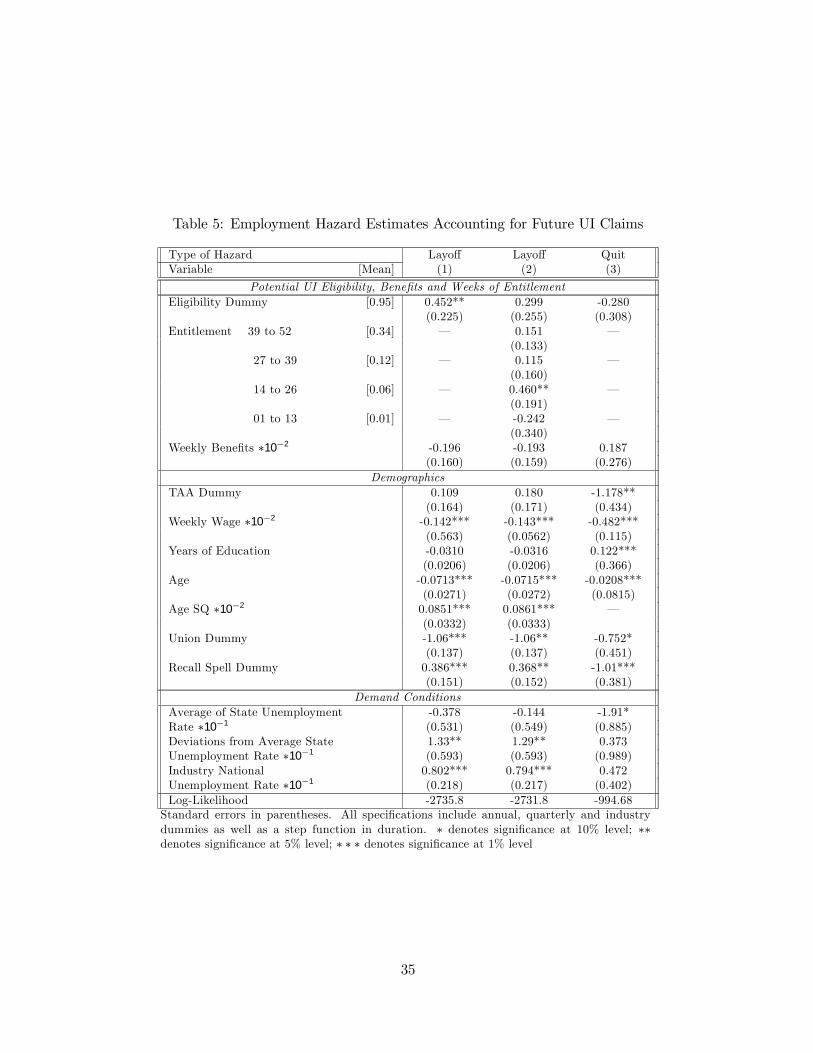
Table 5: Employment Hazard Estimates Accounting for Future UI Claims
Type of Hazard Layoff Layoff QuitVariable [Mean] (1) (2) (3)
Potential UI Eligibility, BeneÞts and Weeks of EntitlementEligibility Dummy [0.95] 0.452** 0.299 -0.280
(0.225) (0.255) (0.308)Entitlement 39 to 52 [0.34] � 0.151 �
(0.133)27 to 39 [0.12] � 0.115 �
(0.160)14 to 26 [0.06] � 0.460** �
(0.191)01 to 13 [0.01] � -0.242 �
(0.340)Weekly BeneÞts ∗10−2 -0.196 -0.193 0.187
(0.160) (0.159) (0.276)Demographics
TAA Dummy 0.109 0.180 -1.178**(0.164) (0.171) (0.434)
Weekly Wage ∗10−2 -0.142*** -0.143*** -0.482***(0.563) (0.0562) (0.115)
Years of Education -0.0310 -0.0316 0.122***(0.0206) (0.0206) (0.366)
Age -0.0713*** -0.0715*** -0.0208***(0.0271) (0.0272) (0.0815)
Age SQ ∗10−2 0.0851*** 0.0861*** �(0.0332) (0.0333)
Union Dummy -1.06*** -1.06** -0.752*(0.137) (0.137) (0.451)
Recall Spell Dummy 0.386*** 0.368** -1.01***(0.151) (0.152) (0.381)
Demand ConditionsAverage of State Unemployment -0.378 -0.144 -1.91*Rate ∗10−1 (0.531) (0.549) (0.885)Deviations from Average State 1.33** 1.29** 0.373Unemployment Rate ∗10−1 (0.593) (0.593) (0.989)Industry National 0.802*** 0.794*** 0.472Unemployment Rate ∗10−1 (0.218) (0.217) (0.402)Log-Likelihood -2735.8 -2731.8 -994.68Standard errors in parentheses. All speciÞcations include annual, quarterly and industrydummies as well as a step function in duration. ∗ denotes signiÞcance at 10% level; ∗∗denotes signiÞcance at 5% level; ∗ ∗ ∗ denotes signiÞcance at 1% level
35
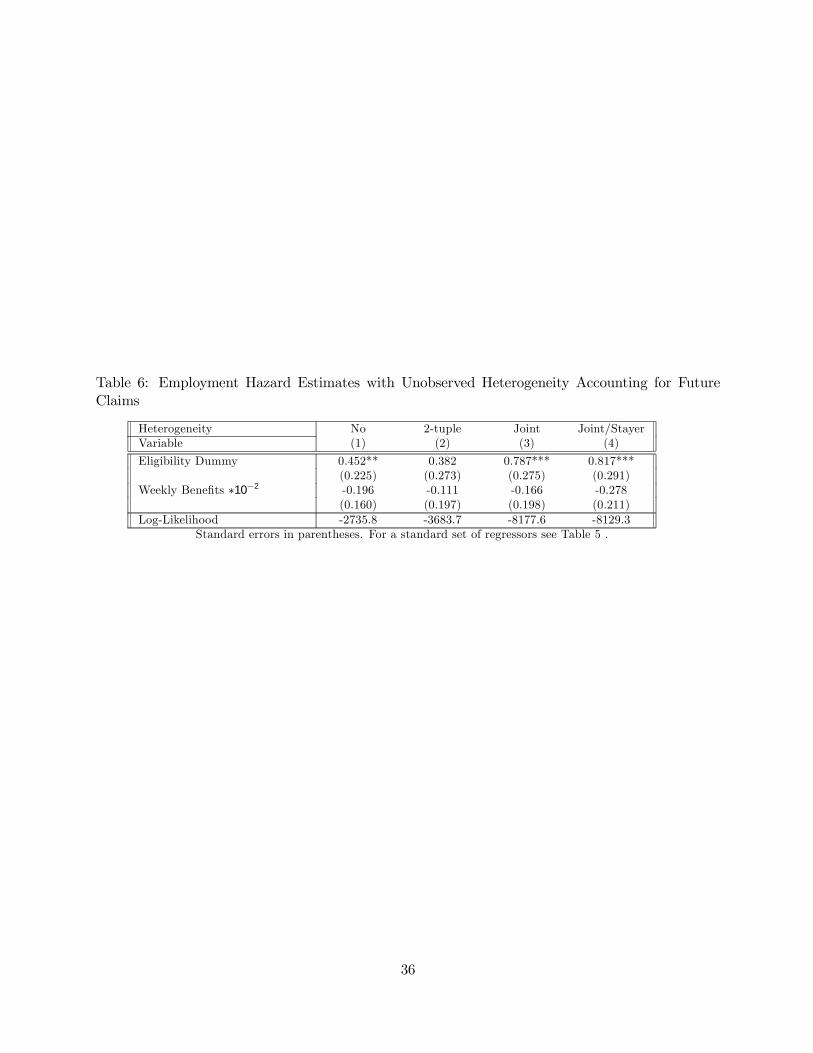
Table 6: Employment Hazard Estimates with Unobserved Heterogeneity Accounting for FutureClaims
Heterogeneity No 2-tuple Joint Joint/StayerVariable (1) (2) (3) (4)
Eligibility Dummy 0.452** 0.382 0.787*** 0.817***(0.225) (0.273) (0.275) (0.291)
Weekly BeneÞts ∗10−2 -0.196 -0.111 -0.166 -0.278(0.160) (0.197) (0.198) (0.211)
Log-Likelihood -2735.8 -3683.7 -8177.6 -8129.3Standard errors in parentheses. For a standard set of regressors see Table 5 .
36
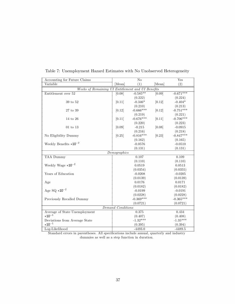
Table 7: Unemployment Hazard Estimates with No Unobserved Heterogeneity
Accounting for Future Claims No YesVariable [Mean] (1) [Mean] (2)
Weeks of Remaining UI Entitlement and UI BeneÞtsEntitlement over 52 [0.08] -0.585** [0.09] -0.671***
(0.222) (0.224)39 to 52 [0.11] -0.346* [0.12] -0.404*
(0.210) (0.213)27 to 39 [0.12] -0.666*** [0.12] -0.751***
(0.219) (0.221)14 to 26 [0.11] -0.676*** [0.11] -0.706***
(0.220) (0.223)01 to 13 [0.09] -0.215 [0.08] -0.0915
(0.216) (0.218)No Eligibility Dummy [0.25] -0.816*** [0.23] -0.847***
(0.162) (0.165)Weekly BeneÞts ∗10−2 -0.0576 -0.0510
(0.131) (0.131)Demographics
TAA Dummy 0.107 0.109(0.110) (0.110)
Weekly Wage ∗10−2 0.0519 0.0513(0.0354) (0.0355)
Years of Education -0.0208 -0.0205(0.0139) (0.0139)
Age 0.0176 0.0171(0.0182) (0.0182)
Age SQ ∗10−2 -0.0199 -0.0191(0.0228) (0.0228)
Previously Recalled Dummy -0.369*** -0.365***(0.0721) (0.0721)
Demand ConditionsAverage of State Unemployment 0.375 0.434∗10−1 (0.407) (0.408)Deviations from Average State -1.32*** -1.35***∗10−1 (0.395) (0.394)Log-Likelihood -4493.0 -4489.5Standard errors in parentheses. All speciÞcations include annual, quarterly and industry
dummies as well as a step function in duration.
37
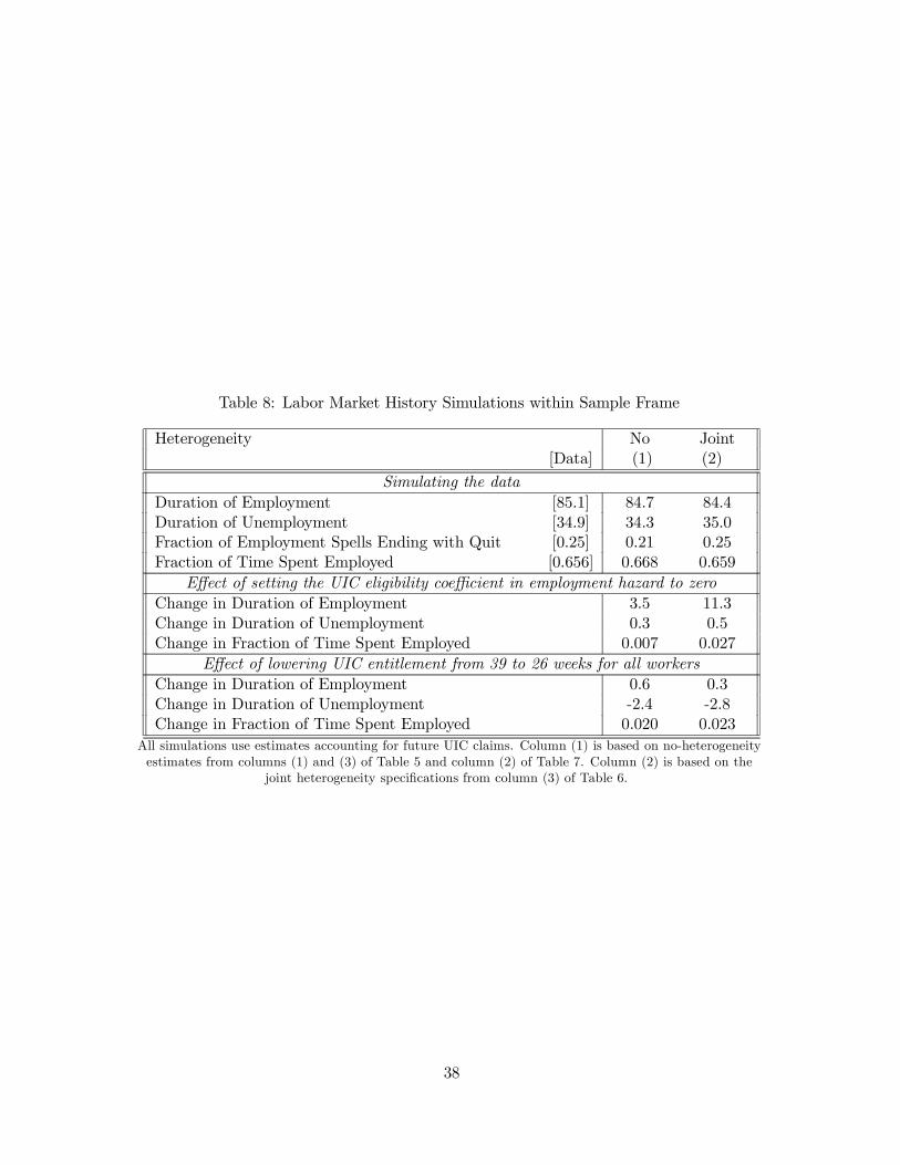
Table 8: Labor Market History Simulations within Sample Frame
Heterogeneity No Joint[Data] (1) (2)
Simulating the dataDuration of Employment [85.1] 84.7 84.4Duration of Unemployment [34.9] 34.3 35.0Fraction of Employment Spells Ending with Quit [0.25] 0.21 0.25Fraction of Time Spent Employed [0.656] 0.668 0.659
Effect of setting the UIC eligibility coefficient in employment hazard to zeroChange in Duration of Employment 3.5 11.3Change in Duration of Unemployment 0.3 0.5Change in Fraction of Time Spent Employed 0.007 0.027
Effect of lowering UIC entitlement from 39 to 26 weeks for all workersChange in Duration of Employment 0.6 0.3Change in Duration of Unemployment -2.4 -2.8Change in Fraction of Time Spent Employed 0.020 0.023
All simulations use estimates accounting for future UIC claims. Column (1) is based on no-heterogeneityestimates from columns (1) and (3) of Table 5 and column (2) of Table 7. Column (2) is based on the
joint heterogeneity speciÞcations from column (3) of Table 6.
38

�������������� ����� �� �������� ������
���� � � ���
211 A. van Soest M. Das X. Gong
A Structural Labour Supply Model with Nonparametric Preferences
5 11/00
212
X. Gong A. van Soest P. Zhang
Sexual Bias and Household Consumption: A Semiparametric Analysis of Engel Curves in Rural China
5 11/00
213
X. Gong A. van Soest E. Villagomez
Mobility in the Urban Labor Market: A Panel Data Analysis for Mexico
1 11/00
214
X. Gong A. van Soest
Family Structure and Female Labour Supply in Mexico City
5 11/00
215
J. Ermisch M. Francesconi
The Effect of Parents’ Employment on Children’s Educational Attainment
5 11/00
216
F. Büchel
The Effects of Overeducation on Productivity in Germany — The Firms’ Viewpoint
5 11/00
217
J. Hansen R. Wahlberg
Occupational Gender Composition and Wages in Sweden
5 11/00
218
C. Dustmann A. van Soest
Parametric and Semiparametric Estimation in Models with Misclassified Categorical Dependent Variables
1 11/00
219
F. Kramarz T. Philippon
The Impact of Differential Payroll Tax Subsidies on Minimum Wage Employment
5 11/00
220
W. A. Cornelius E. A. Marcelli
The Changing Profile of Mexican Migrants to the United States: New Evidence from California and Mexico
1 12/00
221
C. Grund �
Wages as Risk Compensation in Germany
5 12/00
222
W.P.M. Vijverberg
Betit: A Family That Nests Probit and Logit
7 12/00
223
M. Rosholm M. Svarer
Wages, Training, and Job Turnover in a Search-Matching Model
1 12/00
224
J. Schwarze
Using Panel Data on Income Satisfaction to Estimate the Equivalence Scale Elasticity
3 12/00
225
L. Modesto J. P. Thomas
An Analysis of Labour Adjustment Costs in Unionized Economies
1 12/00
226
P. A. Puhani�
On the Identification of Relative Wage Rigidity Dynamics: A Proposal for a Methodology on Cross-Section Data and Empirical Evidence for Poland in Transition
4/5 12/00
227
L. Locher�
Immigration from the Eastern Block and the former Soviet Union to Israel: Who is coming when?
1 12/00
228
G. Brunello S. Comi C. Lucifora
The College Wage Gap in 10 European Countries: Evidence from Two Cohorts
5 12/00
229
R. Coimbra T. Lloyd-Braga L. Modesto
Unions, Increasing Returns and Endogenous Fluctuations
1 12/00
230
L. Modesto
Should I Stay or Should I Go? Educational Choices and Earnings: An Empirical Study for Portugal
5 12/00
231
G. Saint-Paul
The Economics of Human Cloning 5 12/00
232
E. Bardasi M. Francesconi
The Effect of Non-Standard Employment on Mental Health in Britain
5 12/00
233
C. Dustmann C. M. Schmidt
The Wage Performance of Immigrant Women: Full-Time Jobs, Part-Time Jobs, and the Role of Selection
1 12/00
234
R. Rotte M. Steininger
Sozioökonomische Determinanten extremistischer Wahlerfolge in Deutschland: Das Beispiel der Eu-ropawahlen 1994 und 1999
3 12/00
235
W. Schnedler
Who gets the Reward? An Empirical Exploration of Bonus Pay and Task Characteristics
5 12/00
236
R. Hujer M. Caliendo
Evaluation of Active Labour Market Policy: Methodological Concepts and Empirical Estimates
6 12/00
237
S. Klasen I. Woolard
Surviving Unemployment without State Support: Unemployment and Household Formation in South Africa
3 12/00
238
R. Euwals A. Börsch-Supan A. Eymann
The Saving Behaviour of Two Person House-holds: Evidence from Dutch Panel Data
5 12/00
239
F. Andersson K. A. Konrad
Human Capital Investment and Globalization in Extortionary States
5 01/01
240
W. Koeniger
Labor and Financial Market Interactions: The Case of Labor Income Risk and Car Insurance in the UK 1969-95
5 01/01
241
W. Koeniger
Trade, Labor Market Rigidities, and Government-Financed Technological Change
2 01/01
242
G. Faggio J. Konings
Job Creation, Job Destruction and Employment Growth in Transition Countries in the 90’s
4 01/01
243
E. Brainerd
Economic Reform and Mortality in the Former Soviet Union: A Study of the Suicide Epidemic in the 1990s
4 01/01
244
S. M. Fuess, Jr. M. Millea
Pay and Productivity in a Corporatist Economy: Evidence from Austria
5 01/01
245
F. Andersson K. A. Konrad
Globalization and Human Capital Formation
5 01/01
246
E. Plug W. Vijverberg
Schooling, Family Background, and Adoption: Does Family Income Matter?
5 01/01
247
E. Plug W. Vijverberg
Schooling, Family Background, and Adoption: Is it Nature or is it Nurture?
5 01/01
248
P. M. Picard E. Toulemonde
The Impact of Labor Markets on Emergence and Persistence of Regional Asymmetries
2 01/01
249
B. M. S. van Praag P. Cardoso
“Should I Pay for You or for Myself?” The Optimal Level and Composition of Retirement Benefit Systems
3 01/01
250
T. J. Hatton J. G. Williamson
Demographic and Economic Pressure on Emigration out of Africa
1 01/01
251
R. Yemtsov
Labor Markets, Inequality and Poverty in Georgia
4 01/01
252
R. Yemtsov
Inequality and Income Distribution in Georgia
4 01/01
253
R. Yemtsov
Living Standards and Economic Vulnerability in Turkey between 1987 and 1994
4 01/01
254
H. Gersbach A. Schniewind
Learning of General Equilibrium Effects and the Unemployment Trap
3 02/01
255
H. Gersbach A. Schniewind
Product Market Reforms and Unemployment in Europe
3 02/01
256
T. Boeri H. Brücker
Eastern Enlargement and EU-Labour Markets: Perceptions, Challenges and Opportunities
2 02/01
257
T. Boeri
Transition with Labour Supply
4 02/01
258
M. Rosholm K. Scott L. Husted
The Times They Are A-Changin’: Organizational Change and Immigrant Employment Opportunities in Scandinavia
1 02/01
259
A. Ferrer-i-Carbonell B. M.S. van Praag
Poverty in the Russian Federation
4 02/01
260
P. Cahuc F. Postel-Vinay
Temporary Jobs, Employment Protection and Labor Market Performance
1/3 02/01
261
M. Lindahl
Home versus School Learning: A New Approach to Estimating the Effect of Class Size on Achievement
5 02/01
262
M. Lindahl
Summer Learning and the Effect of Schooling: Evidence from Sweden
5 02/01
263 N. Datta Gupta N. Smith
Children and Career Interruptions: The Family Gap in Denmark
5 02/01
264 C. Dustmann Return Migration, Wage Differentials, and the
Optimal Migration Duration 1 02/01
265 M. Rosholm
M. Svarer
Structurally Dependent Competing Risks
1 02/01
266 C. Dustmann O. Kirchkamp
The Optimal Migration Duration and Activity Choice after Re-migration
1 02/01
267 A. Newell
The Distribution of Wages in Transition Countries
4 03/01
268 A. Newell B. Reilly
The Gender Pay Gap in the Transition from Communism: Some Empirical Evidence
4 03/01
269 H. Buddelmeyer
Re-employment Dynamics of Disabled Workers
3 03/01
270 B. Augurzky
C. M. Schmidt
The Evaluation of Community-Based Interventions: A Monte Carlo Study
6 03/01
271 B. Augurzky
C. M. Schmidt
The Propensity Score: A Means to An End 6 03/01

272 C. Belzil J. Hansen
Heterogeneous Returns to Human Capital and Dynamic Self-Selection
5 03/01
273 G. Saint-Paul
Distribution and Growth in an Economy with Limited Needs
5 03/01
274 P. J. Pedersen N. Smith
Unemployment Traps: Do Financial Dis-incentives Matter?
3 03/01
275 G. S. Epstein T. Lecker
Multi-Generation Model of Immigrant Earnings: Theory and Application
1 03/01
276 B. Amable D. Gatti
The Impact of Product Market Competition on Employment and Wages
5 03/01
277 R. Winter-Ebmer Evaluating an Innovative Redundancy-Retraining
Project: The Austrian Steel Foundation
6 03/01
278 T. M. Andersen
Welfare Policies, Labour Taxation and Inter-national Integration
2 04/01
279 T. M. Andersen
Product Market Integration, Wage Dispersion and Unemployment
2 04/01
280 P. Apps R. Rees
Household Saving and Full Consumption over the Life Cycle
7 04/01
281 G. Saint-Paul
Information Technology and the Knowledge Elites
5 04/01
282 J. Albrecht A. Björklund S. Vroman
Is There a Glass Ceiling in Sweden?
5 04/01
283 M. Hagedorn A. Kaul V. Reinthaler
Welfare Analysis in a Schumpeterian Growth Model with Capital
7 04/01
284 H. Rapoport A. Weiss
The Optimal Size for a Minority
1 04/01
285 J. Jerger C. Pohnke A. Spermann
Gut betreut in den Arbeitsmarkt? Eine mikroökonometrische Evaluation der Mannheimer Arbeitsvermittlungsagentur
5 04/01
286 M. Fertig C. M. Schmidt
First- and Second-Generation Migrants in Germany –What Do We Know and What Do People Think
1 04/01
287 P. Guggenberger A. Kaul M. Kolmar
Efficiency Properties of Labor Taxation in a Spatial Model of Restricted Labor Mobility
3 04/01
288 D. A. Cobb-Clark
Getting Ahead: The Determinants of and Payoffs to Internal Promotion for Young U.S. Men and Women
5 04/01
289 L. Cameron
D. A. Cobb-Clark
Old-Age Support in Developing Countries: Labor Supply, Intergenerational Transfers and Living Arrangements
3 04/01
290
D. A. Cobb-Clark M. D. Connolly C. Worswick
The Job Search and Education Investments of Immigrant Families
1 04/01
291
R� T. Riphahn
Cohort Effects in the Educational Attainment of Second Generation Immigrants in Germany: An Analysis of Census Data
1 05/01
292
E. Wasmer
Between-group Competition in the Labor Market and the Rising Returns to Skill: US and France 1964-2000
5 05/01
293
D. Cobb-Clark T. F. Crossley
Gender, Comparative Advantage and Labor Market Activity in Immigrant Families
1 05/01
294
Š. Jurajda
Estimating the Effect of Unemployment Insurance Compensation on the Labor Market Histories of Displaced Workers
3 05/01
�
An updated list of IZA Discussion Papers is available on the center‘s homepage �����������.


