
ESTIMATING LABOUR SUPPLY ELASTICITIES IN THAILAND
USING PERSONAL INCOME TAX STRUCTURES
WARN N. LEKFUANGFU*
This version: 14 FEBRUARY 2017
Abstract
We provide estimations of labour supply elasticities of wage earners in the
case of Thailand. Built upon Blundell, Duncan and Meghir (1998), our
identification strategy develops grouping estimators to address
endogeneity of preference for work. We exploit changes in personal
income tax codes across the years as an exogenous within-group variation
and obtain three types of elasticities of labour supply at the intensive
margins. Thai workers response to wage incentive and unearned income
consistently to the classic theory of labour supply. Workers with very
young child are most responsive to changes of monetary incentives.
Keywords: Labour supply, personal income tax, group-estimator,
elasticity, Thailand
JEL: H24, J2
*Chulalongkorn University and Centre for Economic Performances, LSE

1. INTRODUCTION
Knowledge of how effort responses to incentives is a key issue for designing optimal policy
interventions (Hausman, 1985; Blundell, Symons and Walker 1988). This paper presents a
robust estimation of labour supply elasticities for Thailand. Our empirical design takes into
account heterogeneity of taste for work, roles of non-wage earning and the classic reverse
causality between earned income and effort (Meghir and Phillips 2010). We begin by
exploring some stylised patterns of labour supply in Thailand over the decades. At the
outlook, the labour participation rates in Thailand look somewhat constant over the past three
decades- near 90 percent for males and 70 percent for females (Figure 1.1). On this account
alone, it may seem that the labour market has been irresponsive to changes of market
fundamentals over time. However, at a more disaggregated level, variations of Thailand’s
labour supply behaviours emerge.
Following Blundell, Bozio and Laroque (2011, 2013), we highlight the difference between
the extensive margin of labour supply (whether or not participate in the labour market) and
the intensive margin of labour supply (hours-of-work in a reference period). Along the age
distribution, mean annual hours per working age capita (from Thailand Labour Force
Survey) resembles the conventional inverted U-shape of other countries (Figure 1.2). Figure
1.3 groups individuals by their birth cohort and shows the life-cycle of the extensive margin
for females and males. Decomposing each birth cohort by education level, Figure 1.4
indicates noticeable differences of the patterns of intensive margins over the life cycle for
primary graduates from other education levels1. In sum, among working-age population in
Thailand, both their labour force participation and hours of work vary by individual’
circumstances and calendar year.
In this paper, our analysis looks at the labour supply elasticities separately for males and
females who are wage earners. Our identification strategy is based on comparing the labour
supply behaviour across different groups- classified by birth cohort and education level. Built
upon Blundell, Duncan and Meghir (1998), our approach exploits three variations in order to
circumvent the issue of effort-incentive endogeneity. First, we rely on the differential growth
of marginal wages between education groups due to returns to schooling or minimum wage
1
See Lekfuangfu (2017) for detailed analysis on the extensive and the intensive margins of labour supply in
Thailand across different characteristics.

policy. Second, we exploit the changes of personal income tax rates over the years. Note that,
recent income tax reforms consist of both the expansion of minimum tax allowance and at the
same time, the reduction of marginal rate for high earners. While tax allowances and
minimum taxable income level are more likely to benefit the low education group, the
lowering of the top rate of person income tax is more advantageous for the high education
group. Third, we rely on multiple changes of the tax codes over the years. Therefore, we
obtain a within-group variation of the changes of marginal incentives. Our estimation also
allows for potential self-selection bias due to the idiosyncratic fixed cost of market
participation (Gronau 1974, Heckman 1974, Cogan 1980).
Our estimation model is based on the static model of labour supply2. With the inclusion of
unearned income, our analysis can estimate three types of elasticity: uncompensated wage
elasticity, unearned income elasticity and compensated wage elasticity (Gruber and Saez
(2002); Blundell and MaCurdy 1999). The data used here is a repeated-cross-sections of
Thailand’s Household Socio-Economic Survey (SES). We focus on the SES during the
period of 2006-2015 where there is available information for wages, hours, consumption, and
household circumstances among wage-earners in the representative households. We find that
the uncompensated wage elasticities are positive. It equals 0.26 for an average female and
0.21 for an average male. Taking into account family composition, individuals without young
children in household are least elastic. Non-labour income elasticities are negative and
significantly smaller. The rise of unearned income reduces the intensive margin of labour
supply across gender and family composition. The Hicksian static elasticities are positive and
larger than the uncompensated Marshallian estimates.
The paper is organised as follows: Section 2 presents a simple static labour supply model
and discuss types of labour supply elasticities. In Section 3, we describe our data, the
structure of personal income tax in Thailand and our empirical models. Section 4 presents
estimation results from the main approach using group estimators. Section 5 concludes.
2
In the model, we assume away the endogenous effect of labour supply of other family members. See
Chaippori (1988, 1992) and Blundell et al (2007) for models and estimations of collective labour supply. In our
analysis, unearned income is calculated from the disparity between earned wage and household consumption.
Therefore, we take labour force of other household members essentially as exogenous of representative agents
in our static model.

2. UNDERSTANDING LABOUR SUPPLY RESPONSES
Our conceptual model follows a standard static, within-period labour supply model. A
representative agent decides how much to consume, and therefore how much hours of work
(𝐻𝑡) she wish to supply at a given wage (𝑊𝑡). She also receives an exogenous amount of
non-labour income (unearned income) (𝑌𝑡) where she puts in zero work hours. The agent has
preferences for leisure so an income effect is of negative sign. The higher the wage rate, the
more hours of work. This is because the substitution effect is positive. We illustrate this
standard framework in Equation 1 as follows:
(1) 𝐻𝑡 = 𝐻(𝑊𝑡, 𝑌𝑡, 𝑋𝑡)
where 𝑋𝑡 is individual characteristics. In the static framework, the wage elasticity
(uncompensated) is defined conventionally as 𝐸𝑈 =𝜕ln(𝐻𝑡)
𝜕ln(𝑊𝑡). The unearned income elasticity is
𝐸𝑌 =𝜕ln(𝐻𝑡)
𝜕ln(𝑌𝑡). Therefore, to derive the compensated Hicksian wage elasticity, which hold
utility constant, we write
(2) 𝐸𝐶 = 𝐸𝑈 −𝑊𝑡𝐻𝑡
𝑌𝑡
𝜕ln(𝐻𝑡)
𝜕ln(𝑊𝑡)
In general, because leisure is a normal good, the Hicksian elasticity is normally larger than
the uncompensated Marshallian elasticity (Blundell and MaCurdy, 1999). Many empirical
studies fail to distinguish between these elasticities. With our empirical design, we will be
able to report all three values, separately for females and males.
Studies on labour supply responses with Thai sample show a dispersion of elasticity. A
number of analysis correct for the selection bias of participation choice. Using the SES of
1981 to estimate female labour supply, Schultz (1990) uses husband wage as proxy for non-
labour income and find that female (uncompensated) wage elasticity is negative. Non-labour
income is found to have larger, negative effect of work hours of married females. In contrast,
with the 2008 Labour Force Survey, Aemkulwat (2012) finds positive own wage elasticity
among self-employ male workers. The closest empirical design to ours is that of Warunsiri
and McNown (2010). They construct a pseudo-cohort from the female sample in the LFS
during 1985-2004 and correct for non-zero wage endogeneity. Without unearned income in

the specification, own wage elasticity for females is found to be negative, with the value of
0.25.
3. EMPIRICAL DESIGN
3.1. The data
The data we use are drawn from Thailand Household Socio-Economic Survey (SES). We
focus on the repeated cross-section of the SES in 2006, 2007, 2009, 2011, 2013 and 2015,
where all necessary information include wages, hours, consumptions and household
composition are available. We can only obtain hours only of household members who are
defined as wage earners. For this our individuals represent approximately 40% of the
population of all working-age persons in the SES.
Our key variable, hours of work, is calculated from the reported hours by selected time
reference. We convert this raw idiosyncratic information into the hours worked on a usual
week, comparable across individuals. From reported wages, overtime and bonus, we calculate
the log of usual weekly earnings. The SES contains information on household food
consumption per capita. From this, we calculate a consumption-base non-wage income by
subtracting per-capital food consumption by the value of wage. Our non-wage income is
preferred to other proxies because it allows us to minimise measurement errors (Blundell,
Ham and Meghir 1988, Arellano and Meghir, 1992, Blundell et al 2007)3 .
Then, we group our sample in 10-year birth-cohorts. To maximise the group cell size, our
sample in the analysis will be restricted to four generations: born in 1950-1959, 1960-1969,
1970-1979 and 1980-1989. Within each birth cohort, we disaggregate working-age persons
by education attainment: primary school or below; middle school, college or higher. Table
3.1 shows the distribution of our sample by education and cohort. The mean labour income
and unearned income are calculated respectively in Figure 3.1. Figure 3.2 plots the difference
of work hours by group. In this analysis, participation equals to one if a working-age person
(aged 15-65) is a wage earner and equals zero if she neither is a wage earner or a part of the
broad labour force.
3
Other choices of non-labour incomes are, for example, spouse earnings (Bourguignon and Magnac 1990,
Heckman 1974), income from rents, benefits and capital (Triest, 1990; Kaiser et al 1992) or stock assets
(Domeji and Floden 2006).

3.2: Personal income tax in Thailand
Followed Blundell, Duncan and Meghir (1998), our identification strategy relies on the
evolution of personal income tax codes over the years. This section will begin by describing
the structure and features of personal income tax in Thailand since the 1980s. And
subsequently, we will elaborate how personal income tax is applied in the analysis.
In Thailand, personal income tax is calculated from the taxable gross annual income.
There are 8 broad assessable income items. For some items, e.g. labour income, there is a
level of “deductible expenses” (representing personal production expenses) from which the
value of assessable income will be subtracted. Finally, the taxable gross income is the total
annual assessable income (net of deductible expenses) minus a collection of deductible
allowances (i.e. mean-tested transfers) and exemption items. The total value of deductible
allowances varies according to (i) family structure (child allowances, spouse allowance,
elderly parent allowance), (ii) labour market status (social security contribution), (iii)
financial investment decisions (life insurance, mortgage, funds), (iv) charitable donations and
(v) temporary tax incentives. In the end, individuals are subjected to personal income tax only
when their taxable gross incomes are above the minimum taxable income level (Thailand
Revenue Department)4.
At present, Thailand’s population is at 67 million, with over 50 percent in the labour force
(NSO, 2016). Out of those, 10 million workers are registered under the Social Security Fund
(Social Security Office, 2016). In recent years, the number of potential personal income tax
payers (those who submit income tax forms) has risen from 8 to 11.5 million. However,
because of all deductibles and minimum taxable income level, there is merely 2 million
individuals who are subjected to non-zero income tax rates (Revenue Office, 2015). Over the
years, there have been some reforms in Thailand’s personal income tax structure. (See
Appendix A.)
During the period of 2006 and 2015, there had been two reforms on personal income tax
structure in Thailand (See Appendix A). In 2007, the base level eligible for tax-exemption
was increased from THB 100,000 net taxable income to THB 150,000. In 2013, there is a
4
At present, Thailand’s tax and welfare system does not have any “phase-in/phase-out” government transfer
policies alas the US’s Earned Income Tax Credit or the UK’s Working Family Tax Credit (Ananapibut, 2012;
Muthitacharoen, 2014). Short-term unemployed receive a fixed-term unemployment benefit if they belong to the
Social Security System. The duration and the size is neither conditioned on working hours in the next job.

series of reduction of marginal tax rates5. Most of all, the top rate on net taxable income
above 4 million (equivalent of 100,000 euro) is reduced from 37 percent to 35 percent. To
check if these changes apply to the SES sample of 2006-2015, first we assign the marginal
tax rate to each individual according her annual wage6. Then, we construct an indicator
variable to take the value of 1 if the worker faces a new marginal rate, compare to the year
before had she earned the same amount of net taxable income. It equals to zero if the
marginal rate stays constant as the previous year.
Table 3.2 shows that individuals from the survey year 2009 and 2013 are exposed to the
changes of the tax codes. A smaller proportion of wage earners is exposed to the 2007 change
than the 2013. Among college graduates, approximately 60 percent of wage earners were
exposed to the change in 2013. Primary school wage earners are the least exposed in both
reforms. Because of the timing of the reforms, wage earners with the same qualification are
not equally exposed to the magnitude of changes of marginal tax rates. 80 percent of female
college graduates are completely unexposed to any changes and over 95% of females with
primary qualification are unaffected. There is a small gender difference. For both male and
female workers, the rate of exposure to income tax code changes varies positively with
education level (Figure 3.3). Our identification strategy will exploit the following changes
occurring within well-defined groups of individuals over the years: (i) base-level of net
taxable income eligible for tax exemption, (ii) tax bands and (iii) marginal tax rates. Given a
fixed family structure, changes in tax allowance as well as tax bands are the key sources of
time-varying factors, which influence the optimal level of gross taxable earnings. Facing
progressive tax rates, individuals may try to manipulate their eventual gross taxable earnings
so that it stays just below the higher rate (Meghir and Phillips 2010). Therefore, an
exogenous change in personal income tax policies may influence the re-evaluation of hours
of work7
5
In 2013, for net taxable income between THB 150,000 to 300,000 is reduced from 10 to 5 percent; for net
taxable income between THB 500,000 to 750,000, the rate is reduced from 20 to 15 percent. For THB 1 million
to 2 million, the rate is down from 25 to 30 percent. 6
Annual wage is calculated own weekly hours multiplied by her own weekly wage rate. We assume 50 weeks
per year for all wage earners in the sample. We subsequently deduct the value by per capita tax deductible
expenses. We let the expenses to vary by person’s gross income. See Appendix A and refer to Anantapibut
(2012) for details for the calculation, based on Thailand personal income tax codes at Year 2008. 7
In addition, the structure of deductible items has remains largely constant. In this paper, we omit three other
categories of deductible: financial investments, donations and temporary economic stimulations. The latter
category demonstrates high variations year-on-year. As Anantapibut (2012) points out, deductible allowances
are key determinants for arriving at the net taxable income. Our analysis acknowledges their importance.
However, due to its complexity, our analysis will abstract this feature from labour supply decisions in our

3.3. Identification strategies
Our reduced-form estimations consist of one main OLS equation and 4 auxiliary equations.
Followed Blundell, Duncan and Meghir (1998) and Meghir and Phillips (2010), our 4
auxiliary equations will account for endogeneous preferences for labour market choices
(Heckman, 1974), self-selection, as well as individual’s behavioural responses to changes in
marginal tax rates.
First, we group individuals within the SES based on the education level obtained and the
birth cohort.8 We have 4 birth cohorts: born in 1950-1959, 1960-1969, 1970-1979 and 1980-
1989. Within each birth cohort, we disaggregate working-age persons by education
attainment: primary school or below; middle school, college or higher. Our analysis will look
at females and males separately, allowing for different optimisations between genders.
In a sub-sample analysis, we also disaggregate our original sample further by family
structure: single or married with children. Note that, we acknowledge that grouping based on
family structure are subjected to composition changes as a result of tax policy responses
(Saez et al, 2012). However, by doing so, our model will account for the nature of Thai
income tax policy, which provides generous transfers based strongly on family structure (see
Appendix Figure A.1). This reflects a dispersion of marginal income tax level faced by
otherwise comparable individuals from different household circumstances.
The key identifying assumptions are the followings: First, for our exclusion restriction, we
assume that group composition is unrelated to tax policy changes. Second, income tax policy
changes are exogenous and not anticipated by the individuals in our sample. Third, labour
supply decisions across all groups are assumed to response homogenously to macro-
economic phenomena. That is the financial year fixed effects are not group-dependent. Forth,
the differences in the preferences across education groups stay time-invariant (Blundell et al
2007). The latter is crucial for the basic exclusion restriction in our main labour supply
equation. For the rank condition, we assume that gross pre-tax earnings change differentially
across the assigned groups. This is verified by the differential returns to education non-
linearly across education qualifications (for Thailand, see Warunsiri and McNown, 2010;
model. An alternative inclusion of time-varying financial deductible allowances may see more responsiveness of
labour supply. Therefore, our elasticities may over-estimate the wage effect. 8
Alternatively, many studies opt for grouping individuals by their tax paying status (see for example Eissa,
1995) or by fertility status (see Eissa and Liebman,1996). As Blundell, Duncan and Meghir (1998) pointed out,
these status can in fact be affected by individual’s preferences. Therefore, the composition of each group can
vary flexibly over different financial years, possibly due to changes in tax policies. In contrast, education and
birth year status are less likely to be manipulated once assigned. As a result, a change in tax policy will not alter
the group’s composition.

Tangtipongkul, 2015) as well as the differential total value of deductible allowances from
financial investments structured by the income tax codes. We specify the optimal labour
supply choice at the intensive margin for individual i as
(3) 𝐻𝑖𝑡 = 𝐺𝑔 + 𝑇𝑡 + 𝐾𝑖𝑡 + 𝛽 ln(𝑤𝑖𝑡) + 𝛽𝑌𝑖𝑡 + 𝑣𝑖𝑡�̂� + 𝑣𝑖𝑡
�̂� + 𝜆𝑖𝑡�̂� + 𝑣𝑖𝑡
�̂� +𝜇𝑖𝑡
where ln(𝑤𝑖𝑡) is the log of endogenous pre-tax weekly wage, 𝑌𝑖𝑡 is unearned income, and is
calculated based on consumption at the survey year t. 𝐾𝑖𝑡 is a vector of observable individual
characteristics, for instance family composition. 𝐺𝑔 is a set of dummies for each specific
education-birth cohort group (omitting the college graduate of the 1980/89 birth cohort). 𝑇𝑡 is
a vector of survey year dummies (omitting the 2015 dummy). We specify 𝑣𝑖𝑡�̂� and 𝑣𝑖𝑡
�̂� as the
estimated residuals accounting for the endogeneity of wage and unearned income,
respectively. 𝜆𝑖𝑡�̂� is the conventional inversed Mills’ ratio from the participation equation
described below (Heckman 1974). Lastly, 𝑣𝑖𝑡�̂� is a residual from the first-stage equation,
which predicts the status of tax change exposure for individual i at time t, compared to the tax
code of t-1.
The first auxiliary equation (Eq. Aux 1) estimates the probability of being a wage earner.
The estimation uses a probit specification with the entire sample of working-age population.
𝑃𝑖𝑡 equals to 1 if an individual is a wage earner and zero if she is elsewhere or not in the
labour markets at all. We use all working-age individuals in the SES for this estimation.
Later, we compute the inversed Mills’ ratio 𝜆𝑖𝑡�̂� from the predicted 𝜀𝑖𝑡
𝑃 in this estimation. Our
excluded variables, �́�𝑖𝑡, are (i) marital status (whether or not lived with a partner) and (ii)
region of residence. The first variable picks up endogeneous participation decision due to
intra-household allocations. The second set of variables is a proxy for regional economic
conditions, which may influence the expected outside option for joining the wage earning
sector.
(Aux 1) 𝑃𝑖𝑡 = 𝐺𝑔 + 𝑇𝑡 + 𝐺𝑔𝑇𝑡+𝐾𝑖𝑡+�́�𝑖𝑡 +𝜀𝑖𝑡𝑃
The second and third auxiliary equations tackle the endogeneity of preferences for work,
effort and incentives. Eq. Aux 2 follows an OLS specification with log of pre-tax wage on
individual characteristics, group dummies, year dummies and the fully interacted group-year

dummies as the excluded variables. To mitigate the problem of unobserved preferences
causing zero wage rate, the equation includes the inversed Mills’ ratio from previously
(Meghir and Phillips, 2010). The sample used in Eq. Aux 2 is all wage earners. For Eq. Aux
3, we run a similar specification to Eq. Aux 2 but without the inversed Mills ratio. Here, 𝑌𝑖𝑡
equals 𝑐𝑜𝑛𝑠𝑢𝑚𝑝𝑡𝑖𝑜𝑛 − 𝑤𝑖𝑡𝐻𝑖𝑡.
(Aux 2) log(𝑤𝑖𝑡) = 𝐺𝑔 + 𝑇𝑡 + 𝐺𝑔𝑇𝑡+𝐾𝑖𝑡 +𝑣𝑖𝑡𝑤 + 𝜆𝑖𝑡
�̂�
(Aux 3) 𝑌𝑖𝑡 = 𝐺𝑔 + 𝑇𝑡 + 𝐺𝑔𝑇𝑡+𝐾𝑖𝑡 +𝑣𝑖𝑡𝑌
The last auxiliary regression (Eq. Aux 4) estimates the probability of being exposed to a
new tax rate. To do this, we impose two main assumptions. First, we assume that tax reforms
are unexpected by the individuals and their choice of labour supply is optimised according to
the tax codes of the previous fiscal year. The second assumption suggests that there is no
immediate group switching in response to the tax reform. That is, individuals would be
unable to switch from the birth cohort initially assigned and neither from the education group.
We estimate the tax code exposure with a probit specification, using the full sample of wage
earners in the SES. We have
(Aux 4) 𝑆𝑖𝑡 = 𝐺𝑔 + 𝑇𝑡 + 𝐺𝑔𝑇𝑡+𝐾𝑖𝑡 +𝑣𝑖𝑡𝑆
with 𝑆𝑖𝑡 is an binary variable which takes the value of 1 if an individual is exposed to the
new marginal tax rate at year t, in comparison to year t-1 when he is assumed to have the
constant net taxable income across the two years. It equals to zero if there is no change of
marginal tax rate for his net taxable income bracket. Note that individuals from the same
group may be assigned a different value of 𝑆𝑖𝑡 if there are some tax policy changes in that
particular financial year. All regressions are robust and cluster at province level.
4. EMPIRICAL RESULTS ON LABOUR SUPPLY ELASTICITIES
We organise the report of the empirical results as follows. First, we present the estimated
elasticities derived from the group-estimation models. Table 4.1 reports the uncompensated
wage elasticities and (unearned) income elasticities for females and males. Table 4.2-Table

4.3 present the estimated coefficients from the models with endogeneity corrections using
personal income tax structure.
4.1. Continuous hours elasticities by gender
Table 4.1 present the mean elasticities derived from the estimated model with endogeneous
corrections in Table 4.2. For each wage earner, her uncompensated wage elasticity is the
estimated parameter on the log wage divided by the weekly hours of work. The unearned
income elasticity is the coefficient on the unearned income multiplied by the value of
unearned income and divided by weekly hours of work.
The uncompensated wage elasticity for average female wage earners is positive, with the
value of 0.243. Male’s wage elasticity is also positive but with slightly smaller value at 0.201.
The gender gap of wage elasticity is consistent with estimates from other countries9. The
positive wage elasticities are in line with standard static framework, indicating a substitute
effect of an increase in monetary incentives. We find the unearned elasticities negative for
both genders. In comparison, the absolute size of unearned elasticities are smaller than the
uncompensated wage. The findings confirm that an increase in non-labour income has
negative effect on the intensive margin of labour supply. However, the effect is small.
Turning to heterogeneous responses, we find the intensive margin of labour supply of
wage earners with young children (aged 0-12) are more responsive than those without (no
children or older children). This is similar for both genders. Our finding is aligned with the
estimation in Blundell, Duncan and Meghir (1998) where they also find mothers with child
aged under 5 years to have the highest wage elasticities. Wage earners with young children
also have the highest unearned income elasticities, with negative sign. This implies that,
compare to other family backgrounds, parents of young children are most willing to drop
their hours of work when their non-labour income rise. True for all genders, wage earners
without children in the household are least responsive to both the changes of wages and non-
labour income. Policy interventions to induce more hours of work should be more effective in
raising the intensive margin among parents of young children. And by comparison, a wage
9
For US, see Mroz (1987) for PSID Female (wage elasticity equals 0.12) and see MaCurdy, Green and Paarsch
(1990) for PSID Male (wage elasticity equals 0.032). For Sweden, female elasticity is 0.389 (Bloomquist et al
1990) and male elasticity is 0.21 (Flood and MaCurdy 1992). See Meghir and Phillips (2010) for the recent
survey.

intervention program rather than a universal benefit initiative are expected to induce more
changes of labour supply behaviours.
Next, we derive the compensated wage elasticities following Equation 2. As seen in
Column 1 in Table 4.1, the Hicksian wage elasticities are larger than the Marshallian for
female wage earners with very small child (aged 0-2). For the rest, the calculated
compensated elasticity, which keep the utility constant, has slightly smaller value.
4.2. The estimated parameters with family structure
Table 4.2 reports the estimated parameters from two specifications: the model with
exogenous wage and the model corrected for endogeneous preferences. We run each
specification separately for females and for males. Demographic controls are included. In all
specifications, standard errors are robust and clustered at province-level. The first and the
third column report the estimated coefficients of the log weekly wage and the unearned
income when they are assumed exogenous. The second and the fourth column present the
revised coefficients with all corrections.
The coefficient of the log wage is bigger once endogeneity is corrected for both genders.
This reflects positive correlation of unobserved variables with hours of work. From Column 2
and 4, the positive value of the inversed Mills’ ratio suggest that individuals who choose to
participate in the labour market as wage earners positively select themselves into the sector.
Under the homogeneous effect specification, the size of the coefficient of the unearned
income is smaller for females than males in the uncorrected OLS. Once endogeneity is
accounted for, males’ coefficient of the unearned income becomes larger. The role of
children in the household becomes smaller and not significant from zero in the endogeneous
specification. Female wage earners without children in the households supply higher
intensive margin of labour supply than others.
Table 4.3 presents the estimations for the model which includes interactions with family
background (age of youngest child in the household). Wage coefficients are all positive,
consistent with the theoretical direction of substitute effects. Similar to the homogeneous
effect specifications, the wage coefficients get bigger once endogeneity is corrected for. The
wage coefficient of females without children is the smallest, suggesting the lowest
responsiveness of their intensive margin in comparison. The largest wage coefficient is found
among female wage earners with the youngest child aged 3-5. For males, the largest value of
wage coefficient is of those with the youngest child aged 0-2. The coefficients of the
unearned income are all negative. The absolute size of the coefficient is the largest for
females with child aged 3-5 and males with child aged 0-2. We find the inversed Mills’ ratio
with a positive sign. Again, this confirms positive selection of individuals to the wage earner
sector. The regression results of all four auxiliary equations can be found in the Appendix.
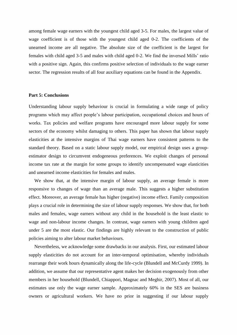
Part 5: Conclusions
Understanding labour supply behaviour is crucial in formulating a wide range of policy
programs which may affect people’s labour participation, occupational choices and hours of
works. Tax policies and welfare programs have encouraged more labour supply for some
sectors of the economy whilst damaging to others. This paper has shown that labour supply
elasticities at the intensive margins of Thai wage earners have consistent patterns to the
standard theory. Based on a static labour supply model, our empirical design uses a group-
estimator design to circumvent endogeneous preferences. We exploit changes of personal
income tax rate at the margin for some groups to identify uncompensated wage elasticities
and unearned income elasticities for females and males.
We show that, at the intensive margin of labour supply, an average female is more
responsive to changes of wage than an average male. This suggests a higher substitution
effect. Moreover, an average female has higher (negative) income effect. Family composition
plays a crucial role in determining the size of labour supply responses. We show that, for both
males and females, wage earners without any child in the household is the least elastic to
wage and non-labour income changes. In contrast, wage earners with young children aged
under 5 are the most elastic. Our findings are highly relevant to the construction of public
policies aiming to alter labour market behaviours.
Nevertheless, we acknowledge some drawbacks in our analysis. First, our estimated labour
supply elasticities do not account for an inter-temporal optimisation, whereby individuals
rearrange their work hours dynamically along the life-cycle (Blundell and McCurdy 1999). In
addition, we assume that our representative agent makes her decision exogenously from other
members in her household (Blundell, Chiappori, Magnac and Meghir, 2007). Most of all, our
estimates use only the wage earner sample. Approximately 60% in the SES are business
owners or agricultural workers. We have no prior in suggesting if our labour supply

elasticities from the wage earners are, to an extent, applicable to other types of job. In sum,
what we have demonstrated here is that wage earners in Thailand adjust their hours of work
consistently with classic labour theory. And that, the presence of young children in household
highly determines their labour supply responses.

REFERENCES
Aemkulwat, C. (2014). Labor Supply of Married Couples in the Formal and Informal Sectors
in Thailand. Southeast Asian Journal of Economics, 2(2), 77-102.
Ananapibut, P. (2012). Tax reforms for more equal Thailand
Arellano, M., & Meghir, C. (1992). Female labour supply and on-the-job search: an empirical
model estimated using complementary data sets. The Review of Economic Studies, 59(3),
537-559.
Blomquist, N. S., & Hansson-Brusewitz, U. (1990). The effect of taxes on male and female
labor supply in Sweden. Journal of Human Resources, 317-357.
Blundell, R., Bozio, A., & Laroque, G. (2011). Labor supply and the extensive margin. The
American Economic Review, 101(3), 482-486.
Blundell, R., Bozio, A., & Laroque, G. (2013). Extensive and intensive margins of labour
supply: work and working hours in the US, the UK and France. Fiscal Studies, 34(1), 1-
29.
Blundell, R., & MaCurdy, T. (1999). Labor supply: A review of alternative
approaches. Handbook of labor economics, 3, 1559-1695.
Blundell, R., Chiappori, P. A., & Meghir, C. (2005). Collective labor supply with children.
Journal of political Economy, 113(6), 1277-1306.
Blundell, R., Chiappori, P. A., Magnac, T., & Meghir, C. (2007). Collective labour supply:
Heterogeneity and non-participation. The Review of Economic Studies, 74(2), 417-445.
Blundell, R., Duncan, A., & Meghir, C. (1992). Taxation in empirical labour supply models:
lone mothers in the UK. The Economic Journal, 102(411), 265-278.
Blundell, R., Duncan, A., & Meghir, C. (1998). Estimating labor supply responses using tax
reforms. Econometrica, 827-861.
Blundell, R., Ham, J., & Meghir, C. (1998). Unemployment, discouraged workers and female
labour supply. Research in Economics, 52(2), 103-131.
Blundell, R., MaCurdy, T., & Meghir, C. (2007). Labor supply models: Unobserved
heterogeneity, nonparticipation and dynamics. Handbook of econometrics, 6, 4667-4775
Bourguignon, F., & Magnac, T. (1990). Labor supply and taxation in France. Journal of
Human resources, 358-389.
Brewer, M., Saez, E., & Shephard, A. (2010). Means-testing and tax rates on
earnings. Dimensions of Tax Design: the mirrlees review, 90-173.
Chiappori, P. A. (1988). Rational household labor supply. Econometrica, 63-90.
Chiappori, P. A. (1997). Introducing household production in collective models of labor
supply. Journal of Political Economy, 105(1), 191-209.
Domeij, D., & Floden, M. (2006). The labor-supply elasticity and borrowing constraints:
Why estimates are biased. Review of Economic dynamics, 9(2), 242-262.
Eissa, N. (1995). Taxation and labor supply of married women: the Tax Reform Act of 1986
as a natural experiment (No. w5023). National Bureau of Economic Research.
Eissa, N., & Liebman, J. B. (1996). Labor supply response to the earned income tax credit.
The quarterly journal of economics, 111(2), 605-637.
Flood, L., & MaCurdy, T. (1992, December). Work disincentive effects of taxes: an empirical
analysis of Swedish men. In Carnegie-Rochester Conference Series on Public Policy (Vol.
37, pp. 239-277). North-Holland.
Gruber, J., & Saez, E. (2002). The elasticity of taxable income: evidence and
implications. Journal of public Economics, 84(1), 1-32.
Heckman, J. (1974). Shadow prices, market wages, and labor supply. Econometrica: journal
of the econometric society, 679-694.
Kaiser, H., van Essen, U., & Spahn, P. B. (1992). Income Taxation and the Supply of Labour
in West Germany: A Microeconometric Analysis With Special Reference to the West
German Income Tax Reforms 1986—1990.
Lekfuangfu (2017). Intensive and extensive margins of labour supply in Thailand, PIER
Working Paper (forthcoming)
MaCurdy, T., Green, D., & Paarsch, H. (1990). Assessing empirical approaches for analyzing
taxes and labor supply. Journal of Human Resources, 415-490.
Meghir, C., & Phillips, D. (2010). Labour supply and taxes. Dimensions of tax design: The
Mirrlees review, 202-74.
Mroz, T. A. (1987). The sensitivity of an empirical model of married women's hours of work
to economic and statistical assumptions. Econometrica: Journal of the Econometric
Society, 765-799.
Muthitacharoen, A. (2014). Negative income tax in Thailand, mimeo
Paweenawat, S. W., & Vechbanyongratana, J. (2015). The impact of a universal allowance
for older persons on labor force participation: The case of Thailand. Population Review,
54(1).
Saez, E., Slemrod, J., & Giertz, S. H. (2012). The elasticity of taxable income with respect to
marginal tax rates: A critical review. Journal of economic literature, 50(1), 3-50.
Schultz, T. P. (1990). Testing the neoclassical model of family labor supply and
fertility. Journal of Human resources, 599-634
Tangtipongkul, K. (2015). Rates of return to schooling in Thailand. Asian Development
Review.
Triest, R. K. (1990). The effect of income taxation on labor supply in the United States.
Journal of Human Resources, 491-516.
Warunsiri, S., & McNown, R. (2010). The returns to education in Thailand: A pseudo-panel
approach. World Development, 38(11), 1616-1625.
Warunsiri, S., & McNown, R. (2010). Female Labor Supply in Thailand: 1985-2004 A
Synthetic Cohort Analysis. Working paper. Institute of Behavioral Science, University of
Colorado at Boulder.

FIGURES
Figure 1.1. Thailand’s labour force participation: by gender
Source: Thailand Labour Force Survey (1985-2015)
Figure 1.2. Mean hours per working age capita: by decade
Source: Thailand Labour Force Survey (1985-2015)

Figure 1.3. Labour participation rate among working-age population
Source: SES (2006-2015)
Figure 1.4. Hours of work by cohort and education
Source: SES (2006-2015)
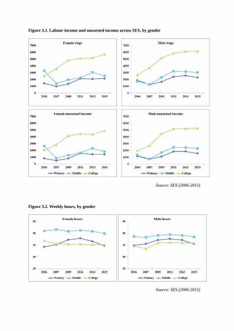
Figure 3.1. Labour income and unearned income across SES, by gender
Source: SES (2006-2015)
Figure 3.2. Weekly hours, by gender
Source: SES (2006-2015)

Figure 3.3. Share of exposure to tax code changes: by gender and education
Source: SES (2006-2015), Record 13.

Tables
Table 3.1: Distribution of the sample
Female Male
Primary Middle College Primary Middle College
% Wage earner 25 31 62 41 44 36
Weekly wage 1723.2 2435.6 5180.2 2055.9 2726.8 5763.1
Weekly
unearned 1122.6 1767.3 4418.2 1399.2 2031.7 4956.6
Weekly hours 46.2 50.9 45.4 46.5 49.0 46.0
Table 3.2. Share of wage earners exposed to the personal income tax reform
Female Male
Primary Middle College Primary Middle College
2006 0.00 0.00 0.00 0.00 0.00 0.00
2007 0.00 0.00 0.00 0.00 0.00 0.00
2009 2.99 7.88 21.20 6.74 11.87 16.91
2011 0.00 0.00 0.00 0.00 0.00 0.00
2013 14.34 38.82 61.48 24.80 43.42 60.18
2015 0.00 0.00 0.00 0.00 0.00 0.00
Mean 3.05 9.84 19.97 5.76 11.52 18.31

Table 4.1: Labour supply elasticities by gender
Compensated Wage Uncompensated Wage Unearned income
Mean Std. Dev. Mean Std. Dev. Mean Std. Dev.
All female 0.234 0.247 0.243 0.265 -0.041 0.248
No children 0.196 0.207 0.203 0.222 -0.038 0.234
Youngest child 0-2 0.321 0.339 0.259 0.283 -0.066 0.402
Youngest child 3-5 0.321 0.339 0.332 0.362 -0.077 0.470
Youngest child 6-12 0.298 0.314 0.309 0.336 -0.068 0.415
Youngest child 12+ 0.252 0.266 0.261 0.285 -0.042 0.255
Observations = 68158
All male 0.194 0.148 0.201 0.188 -0.037 0.174
No children 0.196 0.150 0.203 0.190 -0.039 0.185
Youngest child 0-2 0.235 0.179 0.282 0.264 -0.077 0.364
Youngest child 3-5 0.235 0.179 0.243 0.228 -0.051 0.239
Youngest child 6-12 0.246 0.188 0.254 0.238 -0.053 0.248
Youngest child 12+ 0.207 0.158 0.214 0.200 -0.038 0.181
Observations = 81528

Table 4.2. Estimation for homogeneous effects of wage and unearned income
Female Male
(i) (ii) (iii) (iv)
Dependent variable: weekly hours of work
Log wage 6.00*** 9.63*** 6.50*** 8.06**
[0.71] [3.05] [0.79] [3.37]
Non-wage income -0.00007* -0.00071 -0.00015** -0.00065*
[0.00003] [0.00076] [0.00004] [0.00038]
No children 1.37*** 0.78*** 0.56 -0.17
[0.17] [0.28] [0.42] [0.33]
Youngest child 0-2 0.03 0.75 0.17 0.36
[0.28] [0.58] [0.22] [0.64]
Youngest child 3-5 -0.82*** -0.43 -0.22 -0.34
[0.16] [0.51] [0.24] [0.46]
Youngest child 6+ -0.40* -0.28 -0.40** 0.00116
[0.16] [0.43] [0.12] [0.36846]
Predicted variables from auxiliary models
Residual wage -5.32* -3.2
[2.85] [3.22]
Residual non-wage income 0.00066 0.00057
[0.00076] [0.00038]
Change in tax rate -2.89 -3.74*
[2.13] [2.10]
Participation in wage sector 1.40*** 3.79***
[0.45] [0.55]
Observations 68,158 68,158 81,528 81,528
Adjusted R-squared 0.15 0.13 0.12 0.09
Notes: Robust standard errors in brackets. *** p<0.01, ** p<0.05, * p<0.1. All specifications include the full set
of time dummies, the group dummies and the full interaction of time and group.

Table 4.3. Estimation for heterogeneous effects of wage and unearned income
Female Male
(i) (ii) (iii) (iv)
Dependent variable: weekly hours of work
Log wage 6.51*** 10.37*** 6.20*** 8.59**
[0.59] [2.84] [0.62] [3.43]
Non-wage income -0.00012* -0.00073 -0.00008* -0.00068*
[0.00005] [0.00076] [0.00004] [0.00039]
No children 12.06*** 17.83*** 2.13 3.25
[2.09] [2.73] [3.04] [3.32]
Youngest child 0-2 -7.92** 1.73 -15.15*** -19.27***
[2.81] [7.20] [3.33] [7.07]
Youngest child 3-5 -22.95*** -21.20*** -12.93*** -8.96
[1.88] [7.27] [2.01] [5.83]
Youngest child 6-12 -10.22** -14.13* -19.01*** -12.06**
[3.93] [8.26] [2.87] [5.10]
Wage Effect
No children -1.44*** -2.30*** -0.18 -0.44
[0.27] [0.37] [0.36] [0.43]
Youngest child 0-2 1.11** -0.07 2.12*** 2.73***
[0.38] [0.94] [0.48] [0.93]
Youngest child 3-5 3.15*** 2.82*** 1.78*** 1.17
[0.28] [0.96] [0.29] [0.76]
Youngest child 6-12 1.35* 1.88* 2.62*** 1.63**
[0.56] [1.11] [0.40] [0.67]
Non-Wage Income Effect
No children 0.00007 0.00006 -0.00005 -0.00002
[0.00005] [0.00005] [0.00004] [0.00005]
Youngest child 0-2 -0.00015** -0.00042*** -0.00023* -0.00069***
[0.00005] [0.00015] [0.00011] [0.00014]
Youngest child 3-5 -0.00054*** -0.00062*** -0.00029** -0.00022**
[0.00008] [0.00012] [0.00008] [0.00009]
Youngest child 6-12 -0.0001 -0.00046** -0.00047*** -0.00025**
[0.00008] [0.00017] [0.00009] [0.00010]
Predicted variables from auxiliary models
Residual wage -4.72* -3.52
[2.61] [3.31]
Residual non-wage income 0.00064 0.00061
[0.00075] [0.00039]
Change in tax rate -3.04 -3.35
[1.94] [2.11]
Participation in wage sector 1.19*** 3.69***
[0.43] [0.55]
Observations 68,158 68,158 81,528 81,528
Adjusted R-squared 0.16 0.13 0.12 0.1
Notes: Robust standard errors in brackets. *** p<0.01, ** p<0.05, * p<0.1. All specifications include the full set
of time dummies, the group dummies and the full interaction of time and group.

25
APPENDIX FIGURES
Figure A.1. Evolution of personal income tax (for net annual income ranged 0-1.2 million THB
in nominal term)
Source: author calculation with Thailand Tax Office’s personal income tax codes.

26
Figure A.2. Proportion of deductible expenses to gross income, by net income bracket
Source: Ananapibut (2012)
Notes that Figure A2 is a modified calculation from the original number in Ananapibut (2012). It
displays the values of deductible allowances by type and net taxable income band- calculated at the
2008 personal income tax codes. The size of aggregate family allowances (child, education, spouse
and elderly parents) are common across income bands. In comparison, it counts as a large proportion
of total allowances amongst low income groups. In contrast, the value of deductibles from donations
and financial investments increase as income rises. It indicates that changing family structure plays a
bigger role in determining an individual’s marginal income tax position for lower income groups. On
the contrary, changes in family circumstances is not a determinant factor for marginal income tax
among high earners.

27
Table Appendix:
Table A1- Female: Estimation for unearned income
Birth cohort
effect Y: 2006 Y: 2007 Y: 2009 Y: 2011 Y: 2013 Y: 2015
Year effect -1,633.95 -371.34 12.51 314.12 488.96 D
[76942885.40] [76942885.44] [1,829.40] [1,890.95] [76942885.41]
Primary B: 1950-1959 -3,297.49 2,570.33 335.5 192.46 300.78 D 733.68
[76942885.42] [2,000.32] [4,622.72] [76942885.44] [76942885.44] [76942885.42]
B: 1960-1969 -2,847.24 1,339.44 D -113.41 -74.1 2.96 826.37
[76942885.44] [4,206.07] [76942885.46] [76942885.46] [4,583.51] [76942885.44]
B: 1970-1979 -2,564.22 1,579.53 D -315.04 -299.77 92.45 115.17
[76942885.44] [4,220.47] [76942885.46] [76942885.46] [4,594.45] [76942885.44]
B: 1980-1989 588.77 -2,008.10 -3,336.16 -3,423.53* D -3,405.97 -2,928.70
[2,046.26] [76942885.43] [76942885.47] [1,824.48] [76942885.44] [2,126.30]
Middle B: 1950-1959 -1,226.50 1,200.89 -172.69 D D -52.02 D
[1,552.79] [76942885.47] [76942885.52] [76942885.44]
B: 1960-1969 -2,572.85 1,959.57 497.63 D 192.69 359.83 770.99
[76942885.45] [4,435.41] [76942885.47] [76942885.47] [4,712.50] [76942885.45]
B: 1970-1979 -692.36 D -1,811.02 -1,840.19 -1,361.21 -1,662.46 -1,005.99
[76942885.40] [4,275.28] [76942885.43] [76942885.43] [2,004.90] [76942885.41]
B: 1980-1989 1,944.09 -4,257.58 -4,650.65 -4,478.97 -4,201.71** -3,777.38
[76942885.40] [4,236.83] [76942885.42] [76942885.42] [1,948.89] [76942885.40]
College B: 1950-1959 6,426.61*** 10,697.70 15,235.87 -3,110.32 -920.55 -2,441.63 D
[893.36] [76942885.70] [76942885.66] [2,066.77] [2,136.80] [76942885.42]
B: 1960-1969 2,228.04 D D -602.12 -409.95 D 696.72
[76942885.42] [76942885.44] [76942885.44] [76942885.42]
B: 1970-1979 250.41 D -250.35 77.37 -221.61 -265.18 1,003.14
[76942885.41] [4,991.52] [76942885.43] [76942885.43] [3,563.10] [76942885.41]
B: 1980-1989 D -1,433.20 -2,591.53 -2,138.65 -1,904.19 -1,535.15 D
[76942885.42] [76942885.45] [1,896.32] [1,952.51] [76942885.41]
Family effect No child Aged 0-2 Aged 3-5 Aged 6-10 Older
195.49 -178.36 -312.05 -119.28 D
[200.59] [303.24] [303.30] [257.23]
Notes: Robust standard errors in brackets. *** p<0.01, ** p<0.05, * p<0.1. All specifications include the full set of time dummies and the
group dummies.

28
Table A1- Male: Estimation for unearned income
Birth cohort
effect Y: 2006 Y: 2007 Y: 2009 Y: 2011 Y: 2013 Y: 2015
Year effect -2,900.51*** 507.43 -798.4 -11,796.70 4,526.61 D
[1,058.63] [63467299.51] [1,540.29] [63467299.56] [63467299.52]
Primary B: 1950-1959 -6,111.16 7,099.05 3,073.02** 4,580.38 16,832.78*** D 4,264.08
[63467299.52] [63467299.53] [1,501.87] [63467299.54] [3,605.49] [63467299.52]
B: 1960-1969 -3,144.50 4,185.64 D 1,494.23 13,466.21*** -2,337.63 1,577.48
[63467299.51] [63467299.52] [63467299.53] [3,300.63] [1,475.86] [63467299.51]
B: 1970-1979 10,477.89 -9,985.53 -13,384.24*** -12,157.87 D -16,781.56*** -12,300.99
[63467299.56] [63467299.57] [3,305.35] [63467299.58] [3,598.18] [63467299.56]
B: 1980-1989 -1,348.92 1,766.38 -1,724.53 10,945.46 -4,737.35 -455.51
[1,551.54] [1,246.72] [63467299.53] [63467299.58] [63467299.54] [1,612.33]
Middle B: 1950-1959 704.2 D -3,555.76 D 13,461.68 -4,804.70 832.46
[1,461.72] [63467299.54] [63467299.58] [63467299.54] [1,614.19]
B: 1960-1969 1,012.63 D -3,996.62 -1,478.87 10,115.72 -6,048.06 -1,034.78
[1,170.52] [63467299.52] [1,287.49] [63467299.57] [63467299.53] [1,245.09]
B: 1970-1979 1,452.94 D -4,395.32 -2,736.49** 9,252.96 -7,183.34 -2,496.24**
[1,098.16] [63467299.52] [1,212.48] [63467299.57] [63467299.53] [1,163.14]
B: 1980-1989 -3,118.65 3,759.48 D 1,741.52 13,330.56*** -2,052.10 1,884.32
[63467299.51] [63467299.52] [63467299.53] [3,306.24] [1,487.32] [63467299.51]
College B: 1950-1959 18,760.93 -13,132.15 D -13,578.17 D -17,241.01*** -11,747.74
[63467299.56] [63467299.65] [63467299.58] [3,591.37] [63467299.56]
B: 1960-1969 -1,179.06 6,047.90 D 4,319.03 16,109.19*** 385.06 5,248.73
[63467299.53] [63467299.58] [63467299.56] [3,811.07] [2,411.97] [63467299.53]
B: 1970-1979 -2,877.47 5,092.70 D 3,294.44 15,461.10*** D 4,963.17
[63467299.52] [63467299.54] [63467299.54] [3,578.97] [63467299.52]
B: 1980-1989 D D -2,109.85 -864.7 10,984.71 -4,737.54 D
[63467299.52] [1,544.00] [63467299.56] [63467299.52]
Family effect No child Aged 0-2 Aged 3-5 Aged 6-10 Older
-219.25* -324.78* -316.01* -524.22*** D
[123.82] [174.35] [183.63] [159.56]
Notes: Robust standard errors in brackets. *** p<0.01, ** p<0.05, * p<0.1. All specifications include the full set of time dummies and the
group dummies.

29
Table A2-Female: Estimation for participation decision
Birth cohort
effect Y: 2006 Y: 2007 Y: 2009 Y: 2011 Y: 2013 Y: 2015
Year effect 0.04 0.14*** 0.10** 0.01 0.05 D
[0.03] [0.04] [0.04] [0.02] [0.03]
Primary B: 1950-1959 -0.44*** 0.08** -0.09*** D 0.06* D 0.06
[0.01] [0.03] [0.03] [0.03] [0.04]
B: 1960-1969 -0.35*** 0.02 -0.10*** D D -0.07*** -0.04**
[0.01] [0.03] [0.03] [0.03] [0.02]
B: 1970-1979 -0.27*** 0.01 0.12*** 0.08*** D -0.06** -0.02
[0.01] [0.03] [0.04] [0.03] [0.03] [0.02]
B: 1980-1989 -0.27*** 0.10*** 0.08*** 0.13***
[0.02] [0.04] [0.03] [0.04]
Middle B: 1950-1959 -0.31*** 0.08** D D D D 0.05
[0.01] [0.03] [0.04]
B: 1960-1969 -0.32*** -0.10*** -0.10*** 0 D D 0.04
[0.01] [0.03] [0.03] [0.02] [0.04]
B: 1970-1979 -0.27*** -0.01 -0.01 -0.02 0.07** D 0.10**
[0.02] [0.02] [0.02] [0.03] [0.03] [0.05]
B: 1980-1989 -0.26*** -0.07*** -0.07*** 0.06* 0.11*** 0.07** 0.13***
[0.03] [0.02] [0.02] [0.03] [0.04] [0.03] [0.04]
College B: 1950-1959 -0.08** -0.25*** D D D 0.06 -0.04
[0.04] [0.02] [0.04] [0.03]
B: 1960-1969 -0.05*** 0.02 D D -0.09** D -0.03
[0.01] [0.03] [0.04] [0.03]
B: 1970-1979 -0.03** D -0.06 -0.06 -0.08* 0.03 -0.04
[0.01] [0.04] [0.04] [0.04] [0.02] [0.03]
B: 1980-1989 D D -0.27*** -0.27*** -0.21*** -0.05** D
[0.02] [0.02] [0.03] [0.02]
Family effect No child Aged 0-2 Aged 3-5 Aged 6-10 Older
0.05*** -0.08*** -0.03*** 0 D
[0.00] [0.00] [0.00] [0.00]
Notes: Robust standard errors in brackets. *** p<0.01, ** p<0.05, * p<0.1. All specifications include the full set of time
dummies and the group dummies.

30
Table A2-Male: Estimation for participation decision
Birth cohort
effect Y: 2006 Y: 2007 Y: 2009 Y: 2011 Y: 2013 Y: 2015
Year effect -0.31*** 0.12*** 0.11*** -0.31*** 0.09*** D
[0.01] [0.04] [0.03] [0.02] [0.03]
Primary B: 1950-1959 -0.41*** 0.36*** D -0.06** D D D
[0.01] [0.01] [0.03]
B: 1960-1969 0.03 0.04** -0.05 -0.35*** -0.38*** -0.32*** D
[0.02] [0.02] [0.04] [0.02] [0.02] [0.02]
B: 1970-1979 0.14*** 0.03 -0.36*** -0.35*** -0.38*** -0.32*** D
[0.02] [0.02] [0.03] [0.02] [0.02] [0.02]
B: 1980-1989 0.22*** -0.36*** 0.31*** -0.36*** -0.28*** D
[0.01] [0.02] [0.02] [0.02] [0.02]
Middle B: 1950-1959 -0.29*** D D D 0.32*** -0.06 D
[0.02] [0.02] [0.04]
B: 1960-1969 -0.23*** D -0.02 -0.08*** 0.32*** -0.08** D
[0.01] [0.04] [0.03] [0.02] [0.03]
B: 1970-1979 0.17*** D -0.07* -0.36*** D -0.37*** -0.32***
[0.02] [0.04] [0.02] [0.02] [0.02]
B: 1980-1989 -0.11*** 0.18*** -0.36*** -0.09*** 0.30*** -0.09*** D
[0.01] [0.02] [0.03] [0.03] [0.02] [0.03]
College B: 1950-1959 -0.08*** 0.39*** D D D -0.10*** D
[0.02] [0.01] [0.03]
B: 1960-1969 -0.09*** 0.38*** D 0.02 0.35*** D 0.07*
[0.04] [0.02] [0.02] [0.03] [0.04]
B: 1970-1979 -0.09*** 0.36*** D D 0.36*** D 0.07**
[0.03] [0.02] [0.02] [0.03]
B: 1980-1989 D D -0.34*** -0.27*** 0.24*** -0.11*** D
[0.02] [0.02] [0.02] [0.03]
Family effect No child Aged 0-2 Aged 3-5 Aged 6-10 Older
0.03*** 0 0 0 D
[0.00] [0.01] [0.01] [0.00]
Notes: Robust standard errors in brackets. *** p<0.01, ** p<0.05, * p<0.1. All specifications include the full set of time
dummies and the group dummies.

31
Table A3-Female: Estimation for the log wage
Birth cohort
effect Y: 2006 Y: 2007 Y: 2009 Y: 2011 Y: 2013 Y: 2015
Year effect -0.93 -0.98*** -0.43 -0.12 -0.39 D
[7,201.83] [0.06] [7,201.83] [0.27] [7,201.83]
Primary B: 1950-1959 -0.04 0.13 D -0.07 -0.23 D D
[0.04] [7,201.83] [7,201.83] [0.27]
B: 1960-1969 0.08 -0.13 0.24*** -0.32 -0.50* 0.05 -0.27***
[0.06] [7,201.83] [0.07] [7,201.83] [0.26] [7,201.83] [0.07]
B: 1970-1979 0.06 -0.16 D -0.41 -0.58** 0.01 -0.37***
[0.06] [7,201.83] [7,201.83] [0.26] [7,201.83] [0.07]
B: 1980-1989 -0.11 -0.09 D -0.35 D -0.01 -0.33***
[0.07] [7,201.83] [7,201.83] [7,201.83] [0.08]
Middle B: 1950-1959 0.6 -0.18 -0.24 D D D D
[7,201.83] [0.14] [7,201.83]
B: 1960-1969 0.41 D D -0.24*** -0.51 D -0.36
[7,201.83] [0.08] [7,201.83] [7,201.83]
B: 1970-1979 0.06 D 0.02 -0.17 -0.33 0.19 -0.13
[7,201.83] [7,201.83] [0.13] [7,201.83] [0.14] [7,201.83]
B: 1980-1989 0.08 D D -0.41 -0.56** -0.02 -0.30***
[0.06] [7,201.83] [0.26] [7,201.83] [0.07]
College B: 1950-1959 1.05*** -0.42 D 0.09 D 0.34 D
[0.27] [7,201.83] [7,201.83] [7,201.83]
B: 1960-1969 0.28** D D 0.49 0.31 0.71 0.42***
[0.14] [7,201.83] [0.29] [7,201.83] [0.14]
B: 1970-1979 0.19 D -0.07 0.11 -0.08 D 0.19
[7,201.83] [7,201.83] [0.15] [7,201.83] [7,201.83]
B: 1980-1989 D 0.03 D 0.06 -0.23 0.24 D
[7,201.83] [7,201.83] [0.27] [7,201.83]
Family effect No child Aged 0-2 Aged 3-5 Aged 6-10 Older
-0.01 0.12*** -0.01 -0.04*** D
[0.01] [0.01] [0.01] [0.01]
Notes: Robust standard errors in brackets. *** p<0.01, ** p<0.05, * p<0.1. All specifications include the full set of time
dummies and the group dummies.

32
Table A3-Male: Estimation for the log wage
Birth cohort
effect Y: 2006 Y: 2007 Y: 2009 Y: 2011 Y: 2013 Y: 2015
Year effect -0.87 -1.48*** -0.40*** 0.08 0.19 D
[4,140.64] [0.12] [0.03] [4,140.64] [4,140.64]
Primary B: 1950-1959 -0.09 0.32 1 0.23 -0.07 D 0.2
[4,140.64] [0.21] [4,140.64] [4,140.64] [0.05] [4,140.64]
B: 1960-1969 0.07 D D -0.21 -0.50** -0.37* -0.11
[4,140.64] [4,140.64] [0.21] [0.21] [4,140.64]
B: 1970-1979 -0.06 D 0.69 -0.22 D -0.39* -0.2
[4,140.64] [4,140.64] [4,140.64] [0.21] [4,140.64]
B: 1980-1989 -0.22 D 0.65 D -0.59*** -0.41** -0.22
[4,140.64] [4,140.64] [0.21] [0.21] [4,140.64]
Middle B: 1950-1959 0.19 D D D 0.32 0.15 0.47
[4,140.64] [0.22] [0.22] [4,140.64]
B: 1960-1969 0.69*** D 0.64 -0.38*** -0.7 -0.63 -0.38***
[0.13] [4,140.64] [0.13] [4,140.64] [4,140.64] [0.13]
B: 1970-1979 -0.02 D D -0.05 -0.36* -0.27 0
[4,140.64] [4,140.64] [0.21] [0.21] [4,140.64]
B: 1980-1989 0 D 0.62 -0.37 -0.64*** -0.52** -0.23
[4,140.64] [4,140.64] [4,140.64] [0.21] [0.21] [4,140.64]
College B: 1950-1959 0.89 D D 0.28 -0.29 D 0.22
[4,140.64] [4,140.64] [4,140.64] [4,140.64]
B: 1960-1969 0.76*** -0.26 D 0.06 -0.43 -0.27 D
[0.03] [4,140.64] [0.04] [4,140.64] [4,140.64]
B: 1970-1979 0.40*** -0.36 D -0.11 -0.43 D -0.02
[0.15] [4,140.64] [0.16] [4,140.64] [0.15]
B: 1980-1989 D D 0.68*** D D -0.3 D
[0.14] [4,140.64]
Family effect No child Aged 0-2 Aged 3-5 Aged 6-10 Older
-0.06*** 0.12*** 0.03*** -0.03*** D
[0.01] [0.01] [0.01] [0.01]
Notes: Robust standard errors in brackets. *** p<0.01, ** p<0.05, * p<0.1. All specifications include the full set of time
dummies and the group dummies.

33
Table A4- Female: Estimation of the exposure to changes of marginal tax rate
Birth cohort
effect Y: 2006 Y: 2007 Y: 2009 Y: 2011 Y: 2013 Y: 2015
Year effect D D 0.89*** D 0.99*** D
[0.00] [0.00]
Primary B: 1950-1959 -0.11*** D D 0.14** D D D
[0.01] [0.06]
B: 1960-1969 -0.11*** D D 0.03 D D D
[0.01] [0.04]
B: 1970-1979 -0.11*** D D 0.05 D D D
[0.01] [0.04]
B: 1980-1989 -0.11*** D D D -0.03 D
[0.01] [0.04]
Middle B: 1950-1959 D D D D D D D
B: 1960-1969 -0.02 D D 0.04 D D D
[0.02] [0.04]
B: 1970-1979 -0.01 D D D D 0.01 D
[0.02] [0.03]
B: 1980-1989 -0.08*** D D D D 0.10** D
[0.01] [0.05]
College B: 1950-1959 -0.02 D D -0.07*** D D D
[0.02] [0.02]
B: 1960-1969 0.03 D D D D -0.04* D
[0.03] [0.02]
B: 1970-1979 0.16*** D D 0.01 D D
[0.04] [0.03]
B: 1980-1989 D D D 0.12*** D 0.18*** D
[0.03] [0.04]
Family effect No child Aged 0-2 Aged 3-5 Aged 6-10 Older
0.02*** -0.01 -0.01 -0.01 D
[0.01] [0.01] [0.01] [0.01]
Notes: Robust standard errors in brackets. *** p<0.01, ** p<0.05, * p<0.1. All specifications include the full set of time
dummies and the group dummies.

34
Table A4- Male: Estimation of the exposure to changes of marginal tax rate
Birth cohort
effect Y: 2006 Y: 2007 Y: 2009 Y: 2011 Y: 2013 Y: 2015
Year effect D D 0.25*** D 0.11*** D
[0.02] [0.03]
Primary B: 1950-1959 0.93*** D D 0.04 D D D
[0.00] [0.03]
B: 1960-1969 0.96*** D D 0.05* D D D
[0.00] [0.03]
B: 1970-1979 0.95*** D D D D -0.01 D
[0.00] [0.03]
B: 1980-1989 0.90*** D D D D -0.01 D
[0.00] [0.03]
Middle B: 1950-1959 0.88*** D D D D D D
[0.00]
B: 1960-1969 0.92*** D D 0.02 D D D
[0.00] [0.03]
B: 1970-1979 0.95*** D D D D 0.02 D
[0.00] [0.03]
B: 1980-1989 0.96*** D D -0.08*** D D D
[0.00] [0.02]
College B: 1950-1959 0.89*** D D -0.13*** D D D
[0.00] [0.01]
B: 1960-1969 0.92*** D D -0.03 D D D
[0.00] [0.03]
B: 1970-1979 0.93*** D D 0 D D D
[0.00] [0.03]
B: 1980-1989 D D D 0.89*** D 0.89*** D
[0.00] [0.00]
Family effect No child Aged 0-2 Aged 3-5 Aged 6-10 Older
0.01** -0.02* 0 -0.01 D
[0.01] [0.01] [0.01] [0.01]
Notes: Robust standard errors in brackets. *** p<0.01, ** p<0.05, * p<0.1. All specifications include the full set of time
dummies and the group dummies.


