
Economic Impacts Resulting from
Implementation of the RFS2 Program
Prepared for:
American Petroleum Institute
Report
July 27, 2015

i
Project Team/Authors
Paul Bernstein, Vice President
Bob Baron, Outside Consultant
Alyssa Lipshultz, Research Assistant
W. David Montgomery, Affiliated Consultant
Mei Yuan, Senior Consultant
The findings contained in this report may contain predictions based on current data and historical
trends. Any such predictions are subject to inherent risks and uncertainties. In particular, actual
results could be impacted by future events that cannot be predicted or controlled, including,
without limitation, changes in business strategies, the development of future products and
services, changes in market and industry conditions, the outcome of contingencies, changes in
management, and changes in law or regulations. Neither API nor NERA accept responsibility
for actual results or future events.
The opinions expressed herein are those of the authors and do not necessarily represent the views
of NERA Economic Consulting or any other NERA consultant.
© NERA Economic Consulting
NERA Economic Consulting
1255 23rd Street NW
Washington, DC 20037
Tel: +1 202 466 3510
Fax: +1 202 466 3605
www.nera.com
ii
Contents
EXECUTIVE SUMMARY ...........................................................................................................1 A. Past and Current Study Methodology ..................................................................................1 B. Results ..................................................................................................................................1 C. Conclusions ..........................................................................................................................2
II. INTRODUCTION..............................................................................................................4 A. 2012 NERA RFS2 Study .....................................................................................................5 B. Current Study: Scope and Study Objectives .......................................................................6
III. BACKGROUND ................................................................................................................7 A. RFS2 ....................................................................................................................................7
1. Nested Mandates ..............................................................................................................7
2. Implementation ................................................................................................................8
3. Waivers ............................................................................................................................9 B. EPA’s 2015 NPRM ..............................................................................................................9
IV. DESCRIPTION OF THE MODELS .............................................................................12 A. Transportation Fuel Model ................................................................................................12
1. The Transportation Fuel Model is designed to Model RFS2 Program
Characteristics ..............................................................................................................12 2. RFS Constraints: ............................................................................................................13 3. Other Model Elements ...................................................................................................13
B. NewERA Macroeconomic Model .......................................................................................14 C. Model Integration...............................................................................................................15
D. Analytical Methodology ....................................................................................................15 E. Model Parameters ..............................................................................................................17
1. Fuel Prices ......................................................................................................................17 2. Supply Elasticities ..........................................................................................................18
3. Demand Elasticities .......................................................................................................19 4. E85 19 5. Upper Bounds on Supply of Various Biofuels ..............................................................20 6. Other Fuel Constraints and Assumptions ......................................................................21
V. RESULTS .........................................................................................................................23 A. Study Results .....................................................................................................................23 B. The Dilemma with RFS2 ...................................................................................................23 C. Macroeconomic Impacts ....................................................................................................24
VI. CONCLUSIONS ..............................................................................................................25
APPENDIX A. DETAILED MODEL DESCRIPTION ..........................................................26 A. Transportation Fuel Model ................................................................................................26
1. Fuel Supply Curves ........................................................................................................26 2. Demand Curves ..............................................................................................................26 4. Transportation Fuel Model is Designed to Model RFS2 Program Characteristics ......27

iii
5. RFS/RIN Constraints .....................................................................................................27
6. Model Formulation ........................................................................................................29 B. NewERA Macroeconomic Model .......................................................................................30
1. Overview of the NewERA Macroeconomic Model ........................................................30
2. Model Data (IMPLAN and EIA) ...................................................................................30 3. Brief Discussion of Model Structure .............................................................................30
APPENDIX B. DETAILED TRANSPORTATION MODEL RESULTS FOR THE
STATUTE SCENARIO ...................................................................................................41

iv
List of Figures
Figure 1: 2015 Gasoline and Diesel Results in Statute Scenario .................................................... 2
Figure 2: Fuel Production and Blending Options for Meeting RFS2 Compliance ......................... 5
Figure 3: Applicable Volumes Specified in the Clean Air Act and the EPA’s Proposed Volume
Requirements (Billion Ethanol-Equivalent Gallons) ........................................................ 10
Figure 4: Comparison of EIA forecasted Biofuel Volumes and EPA’s Proposed Volume
Requirements (Billion Ethanol-Equivalent Gallons) ........................................................ 11
Figure 5: Baseline Fuel Price Ratios for Blended Gasoline and Diesels (Ratio on a GGE Basis of
Biofuel to Conventional Fuel) .......................................................................................... 18
Figure 6: Fuels Institute’s Top Quartile and EIA’s E85 Sales Forecasts (Billion Gallons) ......... 20
Figure 7: Maximum level of biofuels (Billion Gallons) .............................................................. 20
Figure 8: 2015 Gasoline and Diesel Results in Statute Scenario .................................................. 23
Figure 9: AEO 2015 Reference Case Fuel Prices (2013$/Gallon) .............................................. 27
Figure 10: EPA’s Formulas for the RFS2 Percentage Mandates ................................................. 28
Figure 11: EPA’s Proposed Rule for RFS standards for 2015 and 2016 ..................................... 29
Figure 12: Circular Flow of Income ............................................................................................ 31
Figure 13: Standard NewERA Model’s Macroeconomic Regions ............................................... 32
Figure 14: NewERA Sectoral Representation in Core Scenarios ................................................. 33
Figure 15: NewERA Household Representation ........................................................................... 34
Figure 16: NewERA Electricity Sector Representation ................................................................ 35
Figure 17: NewERA Trucking and Commercial Transportation Sector Representation .............. 36
Figure 18: NewERA Other Production Sector Representation ..................................................... 36
Figure 19: NewERA Resource Sector Representation ................................................................. 37
Figure 20: Quantities in Statute Scenario (Billion Gallons, Unless Otherwise Noted) ................ 41
Figure 21: Cost to Consumer in Statute Scenario (2013$/gallon) ................................................ 42

v
Terminology
AEO
Annual Energy Outlook. An annual publication from the EIA that
offers projections that can be used as a basis for examination and
discussion of energy production, consumption, technology and market
trends and the direction they may take in the future. This study used
AEO2015.
BOB Blendstock for Oxygenate Blending
CARB California Air Resources Board
CGE Computable General Equilibrium
Biodiesel
A type of biomass-based diesel comprised of mono-alkyl esters of long
chain fatty acids derived from vegetable oils or animal fats, and
meeting the requirements of ASTM D 6751. A blend of biodiesel fuel
with petroleum-based diesel fuel designated BXX, where XX
represents the volume percentage of biodiesel fuel in the blend.
Biomass-Based Diesel Includes biodiesel and renewable diesel
Biofuel Producer or
Importer
Generator of RINs at the point of biofuel production or the port of
importation
Blending Percentage
Standard
Ratio of renewable fuel volumes required by RFS2 and the total
gallons of gasoline and diesel fuel that will be sold in the
upcoming year
EIA Energy Information Administration
EISA ‘07 Energy Independence and Security Act of 2007
EPA United States Environmental Protection Agency
E0 Neat gasoline; 100% petroleum gasoline, does not contain ethanol
E10 A gasoline blend containing 10 percent ethanol by volume (E10)
E85
An ethanol/gasoline fuel blend containing a relatively high percentage
of ethanol by volume and a relatively low percentage of petroleum
hydrocarbons by volume. While its name connotes a blend of 85%
ethanol and 15% gasoline, the ethanol content of E85 is seasonally
adjusted to meet ASTM recommended specifications and to improve
vehicle cold-start and warm-up performance. Following the EIA’s
practice, we will analyze E85 sales under the assumption that fuel sold
as E85 consists of 74% ethanol and 26% gasoline by volume on a year-
round average basis.
FFV Fuel Flexible Vehicles: certified to use ethanol/gasoline blends
containing up to 85 percent volume ethanol

vi
NewERA NERA’s proprietary macroeconomic model
NPRM EPA’s 2015 Notice of Proposed Rule Making
Obligated Party Obligated Party Companies that produce and/or import gasoline and/or
diesel fuel
RFS2 Renewable Fuel Standard Per Energy Independence and Security Act
of 2007
RINs Renewable identification numbers (Credits for compliance with RFS2)
RVO Renewable Volume Obligation
Statute Scenario
Total renewable fuels and advanced biofuels at EISA ’07 statute levels
and biomass-based diesel at June 2015 NPRM levels for 2015-2017 and
held constant at 2017 levels for 2018-2022. Cellulosic biofuel set at
June 2015 NPRM levels for 2015-2016 and held at 2016 volume for
2017-2022
STEO EIA’s Short Term Energy Outlook

1
EXECUTIVE SUMMARY
The American Petroleum Institute (API) commissioned NERA Economic Consulting (NERA) to
conduct a study of the potential transportation sector and macroeconomic impacts of the U.S.
Renewable Fuel Standard (RFS2) Program on the economy. NERA1 relied upon publically
available information and NERA’s proprietary economic modeling to develop the analysis.
A. Past and Current Study Methodology
In 2012, NERA released its first study of RFS2.2 In that study, NERA analyzed the economic
and compliance issues related to the implementation of RFS2. That study, like the current study,
assumed the renewable fuel volume obligation (RVO) for total renewable fuel, advanced
biofuels, and biomass-based diesel in each year would be equal to the volumes specified in the
Energy Independence and Security Act of 2007 (EISA ‘07).3
In this study, NERA similarly considers the following scenario:
Statute Scenario: Total renewable fuel and advanced biofuel volumes are set equal to
EISA ’07 statute levels. Biomass-based diesel volumes are set equal to June 2015 NPRM
volumes for 2015-2017 and held constant at 2017 levels for 2018-2022. Cellulosic
biofuel volumes are set equal to the June 2015 NPRM volumes for 2015-2016 and held at
the 2016 volume for 2017-2022.
B. Results
As shown in Figure 1, when the required volume of total renewable fuel is equal to the EISA ’07
statute requirement, the Statute Scenario exhibits a decrease in gasoline and diesel demand vs.
EIA and outrageously high consumer costs that are evident immediately, i.e, in 2015. The 2015
statutory requirement would require about 30%4 more RINs to be generated than were generated
in 2014. In order to achieve the associated required blending percentage for obligated parties
with the supply of available RINs requires about a 30% reduction in gasoline and diesel volumes
from expected demand in 2015. To achieve this reduction in gasoline and diesel demand
requires that costs increase by roughly $90 and $100 per gallon more than today’s costs,
respectively.
1 All results and observations are based on information at the time of the report. To the extent that additional
information becomes available or the factors upon which our analysis is based change, our opinions could
subsequently be affected.
2 Economic Impacts Resulting from Implementation of RFS2 Program, Prepared for the American Petroleum
Institute, October 2012.
3 The study assumed that cellulosic biofuel requirements were waived each year.
4 EPA proposes 15.9 billion RINs for 2014. The statute requires 20.5 billion RINs in 2015.

2
Figure 1: 2015 Gasoline and Diesel Results in Statute Scenario
Volume
(Billion Gallons)
Cost to Consumer
($/Gallon)
Gasoline5 93 $92
Diesel 40 $103
Source: NERA analysis.
The price increases in gasoline and diesel are accompanied by a reduction in demand for the
transportation fuels. Since the transportation sector is interconnected with other sectors in a way
that the transportation services are consumed by other sectors, the fuel cost increase creates the
spillover effects that ripple through the economy. Higher diesel fuel costs increase the cost to
move raw materials and finished goods around the country, thus eventually making everything
that directly or indirectly depends on transportation services more costly. Likewise the higher
gasoline prices leave consumers with less disposable income. As a result of these impacts,
consumption of goods and services declines. All of these impacts lead to severe economic harm.
C. Conclusions
Based upon NERA’s modeling of the transportation sector and the overall economy for
implementing the RFS2 biofuel volume requirements, NERA concludes:
In 2015 and beyond, it is not feasible to achieve the statute volumes of total renewable
fuel required under EISA ‘07. The current level of gasoline demand, the blend wall
limiting the share of ethanol that can be blended into the gasoline pool, and the lack of
non-ethanol biofuels limit the market potential for total renewable biofuels. Similarly the
current market potential for higher ethanol content gasoline like E85 and E15 is too small
to have an immediate impact on the amount of ethanol that the gasoline market can
absorb.
Only by the EPA invoking its two different waiver authorities6 to issue a waiver for
cellulosic ethanol and the same deduction for the total renewable biofuels and advanced
biofuel volumes requirements as well as a general waiver for both advanced biofuels and
total renewable fuels would allow the RFS2 to be feasible.
NERA’s conclusion that it is infeasible to achieve the statute volumes for total renewable
fuels in 2015 and beyond is consistent with NERA’s findings from its 2012 study, which
also found that if the EPA retained the EISA ’07 statute volumes, severe economic harm
5 For this figure, gasoline includes E0, E10, and E85. Therefore, the gasoline price is the weighted average price of
E0, E10, and E85.
6 The cellulosic ethanol waiver allows EPA to reduce applicable volumes for cellulosic biofuels and apply the same
reduction to the total renewable biofuels and advanced biofuel volumes requirements. The general waiver allows
EPA to reduce volumes for any renewable fuel if there is inadequate supply.

3
would result in the 2015 to 2016 time frame. Infeasibility has not occurred yet because
EPA has recognized the blend wall and is proposing volumes below the statute levels.
Economic harm: When the required biofuel volume standards are too severe, as with the statute
scenario, the market becomes disrupted because there are an insufficient number of RINs to
allow compliance. “Forcing” additional volumes of biofuels into the market beyond those that
would be “absorbed” by the market based on economics alone at the levels required by the
statute scenario will result in severe economic harm.

4
II. INTRODUCTION
The American Petroleum Institute (API) commissioned NERA Economic Consulting (NERA) to
analyze the potential impacts on the transportation fuels market and the U.S. economy resulting
from complying with the statutory volumes under the Renewable Fuel Standard (RFS2)7 through
2022. NERA relied upon publically available information and NERA’s proprietary economic
modeling to develop the analysis.
The RFS2 requires transportation fuel producers and importers (obligated parties) to incorporate
specified volumes and categories of biofuels into their products annually. These mandates
increase each year and collectively require the use of 36 billion gallons of renewable fuels in
2022. Each year, the EPA is supposed to assess for the next year whether or not the statutory
volumes prescribed under EISA ‘07 are achievable. If not, the EPA has the authority to lower
the annual fuel mandate for each class of renewable fuel. Each year the annual total renewable
fuel volume mandate is calculated as a percentage of the nation’s total projected fuel
consumption for the upcoming year. The renewable fuel volume obligation (RVO) for each
obligated party is calculated by applying that percentage to the total annual volume of gasoline
and diesel produced or imported by each obligated party during that year. Compliance with the
RFS2 each year is demonstrated through “Renewable Identification Numbers” (RINs) which are
unique identifiers attached to every gallon of renewable fuel produced or imported. Obligated
parties submit RINs as evidence of their compliance with the RVO.
Figure 2 lists the four primary mechanisms that obligated parties can use to comply with the
RFS2. To comply with the RFS2 mandates, obligated parties have increased production of E10
and E85 while minimizing production of E0 (pure gasoline). As the RFS2 mandated volumes for
renewable fuels increase, however, these mechanisms reach their limit.
7RFS2 was part of the Energy Independence and Security Act of 2007 (“EISA ‘07”).

5
Figure 2: Fuel Production and Blending Options for Meeting RFS2 Compliance
Compliance Mechanism Limitation
Minimize production of E0 Demand for E0 will not completely disappear due to
customer demand
Increase production of E85 Demand for E85 will remain low due to limited E85
infrastructure, E85’s low fuel economy, and limited
consumer preference for E85
Increase use of biomass-based
diesel
The available volume of biomass-based diesel is relatively
small compared to the overall RFS2 requirement. The
infrastructure to blend biomass-based diesel is limited.
Produce and market E15 Market penetration of E15 will be limited by vehicle
warranty, retail infrastructure, misfueling, and general
liability issues
When obligated parties exhaust these methods of compliance, they will eventually be forced to
either decrease their production volumes or export product in order to reduce their individual
biofuel obligation and meet RFS2 volume percentage requirements. These market shifts will
initially result in a tightening of the diesel fuel supply followed by subsequent years of
reductions in both the gasoline and diesel fuel supply. The shrinking domestic petroleum fuel
supply coupled with expanding RFS2 requirements would result in making compliance
increasingly more difficult and lead to significant negative economic impacts.
This process repeats itself yearly. As domestic supply continues to decline, the blending
percentage obligation becomes increasingly unattainable. Obligated parties rely on RINs
acquired and carried forward from earlier years to meet compliance obligations.
A. 2012 NERA RFS2 Study
In 2012, NERA released its first study of RFS2.8 In that study, NERA analyzed the economic
and compliance issues related to the implementation of RFS2. That study, like the current study,
assumed that in each year the renewable fuel volume obligation (RVO) for total renewable fuel,
advanced biofuels, and for biomass-based diesel would be equal to the volumes specified in
EISA ‘07.9 In other words, the study assumed that the EPA decided not to exercise its authority
to reduce the RVO requirements in any year for three of the four biofuel categories; the only
exception was cellulosic biofuel. The study found that if the RVO remained at the levels called
for in EISA ‘07 that RFS2 would likely become infeasible in three to four years (2015 or 2016),
8 Economic Impacts Resulting from Implementation of RFS2 Program, Prepared for the American Petroleum
Institute, October 2012.
9 The study assumed that cellulosic biofuel requirements were waived each year.

6
resulting in significant harm to the U.S. economy. Since the time of our first study, the EPA in
subsequent rulemaing(s) acknowledged the existence of the blend wall10
and that the statute
requirement for renewable fuel volumes is infeasible.11
As a result, the EPA has proposed lower
targets in its current Notice of Proposed Rulemaking (NPRM).
B. Current Study: Scope and Study Objectives
API retained NERA Economic Consulting (NERA) to update its analysis of the potential impacts
on the transportation fuels market and the U.S. economy resulting from complying with the
RFS2 statutory volumes. NERA relied upon publically available information and NERA’s
proprietary economic modeling to develop the analysis.
In this study, NERA considers the following scenario:
Statute: Total renewable fuel and advanced biofuel volumes are set equal to EISA ’07
statute levels. Biomass-based diesel volumes are set equal to June 2015 NPRM volumes
for 2015-2017 and held constant at 2017 levels for 2018-2022. Cellulosic biofuel
volumes are set equal to the June 2015 NPRM volumes for 2015-2016 and held at the
2016 volume for 2017-2022.
NERA used updated versions of its two proprietary models that were used in the earlier study:
NERA’s transportation fuel model and the NewERA macroeconomic model. These models were
run12
to quantify the economic impacts from implementation of the RFS2. Specifically, the
transportation fuel model estimates the amount of fuel produced for and consumed by the
transportation sector and explicitly estimates the demand for E0, E10, E85 and blended diesel.
The NewERA macroeconomic model13
simulates all economic interactions in the U.S. economy,
including those among industry, households, and the government.
10
“The proposal seeks to put the RFS program on a steady path forward – ensuring the continued growth of
renewable fuels while recognizing the practical limits on ethanol blending, called the ethanol ‘blend wall.’” EPA
Proposes 2014 Renewable Fuel Standards, 2015 Biomass-Based Diesel Volume, Office of Transportation and Air
Quality, EPA-420-F-13-048, p. 1, November, 2013. 11
“Due to constraints in the fuel market to accommodate increasing volumes of ethanol, along with limits on the
availability of non-ethanol renewable fuels, the volume targets specified by Congress in the Clean Air Act for
2014, 2015, 2016 cannot be achieved.” EPA Proposes Renewable Fuel Standards for 2014, 2015, and 2016, and
the Biomass-Based Diesel Volume for 2017, Office of Transportation and Air Quality, EPA-420-F-15-028, p. 2,
May, 2015.
12 The macroeconomic model was connected to the transportation fuel model through a one-way link in which the
macroeconomic model incorporated the fuel cost increases of the transportation model.
13 The NewERA macroeconomic model uses the resulting scenario fuel prices from the transportation fuel model.
Then the NewERA macroeconomic model is run to assess the economy wide impacts of the changes in fuel prices.
Since the transportation model becomes infeasible in 2015 in the Scenario, we could not run the NewERA
macroeconomic model past 2015.

7
III. BACKGROUND
A. RFS2
Congress first established a Renewable Fuel Standard (RFS) in 2005 with the enactment of the
Energy Policy Act of 2005 (EPACT). Two years later, Congress passed the Energy
Independence and Security Act of 2007 (EISA ‘07) which superseded and greatly expanded the
biofuels blending mandate. This expanded RFS is referred to as RFS2, which applies to all
transportation fuel used in the United States—including diesel fuel intended for use in highway
motor vehicles, non-road, locomotive, and marine diesel.14
RFS2 introduces four new major
distinctions from RFS:
1. RFS2 increases the mandated usage volumes and extends the time frame over which the
volumes ramp up to 2022;
2. RFS2 subdivides the total renewable fuel requirement into four separate but nested
categories—total renewable fuels, advanced biofuels, biomass-based diesel, and
cellulosic biofuel—each with its own volume requirement or standard;
3. Biofuels qualifying under each nested category must achieve certain minimum thresholds
of lifecycle greenhouse gas (GHG) emission performance, with certain exceptions
applicable to existing facilities; and
4. All renewable fuel must be made from feedstocks that meet the new definition of
renewable biomass, including certain land use restrictions.
1. Nested Mandates
Because of the nested nature of the biofuel categories, any renewable fuel that meets the
requirement for cellulosic biofuels or biomass-based diesel is also valid for meeting the overall
advanced biofuels requirement. Thus, any combination of cellulosic biofuels or biomass-based
diesel would count toward the advanced biofuels mandate, thereby reducing the potential need
for imported sugarcane ethanol to meet the “other” advanced biofuels mandate. Similarly, any
renewable fuel that meets the requirement for advanced biofuels is also valid for meeting the
total renewable fuels requirement. As a result, any combination of cellulosic biofuels, biomass-
based diesel, or imported sugarcane ethanol that exceeds the advanced biofuel mandate would
reduce the potential need for corn-starch ethanol to meet the overall mandate.
14
Renewable fuels used in ocean-going vessels cannot count toward RFS2 mandates. Renewable fuels used in
heating oil and jet fuel do count towards the RFS mandates.

8
2. Implementation
Under EISA ‘07, the U.S. Environmental Protection Agency (EPA) is responsible for
implementing regulations to ensure that transportation fuels sold in the United States contain a
minimum volume of renewable fuels in accordance with the four nested volume mandates of the
RFS2. Compliance with the RFS2 is demonstrated by the use of RINs.15
A RIN is generated by a biofuel producer or importer at the point of biofuel production or the
port of importation. Each gallon of ethanol generates one RIN. Because of the higher energy
content per gallon than ethanol, biodiesel generates 1.5 RINs per gallon; similarly renewable
diesel generates between 1.5 and 1.7 RINs per gallon. RIN generators must register with the
EPA. After a RIN is created by a biofuel producer or importer, it must be reported to the EPA.
RINs are transferable.
Congress has determined the total renewable fuel volume that must be incorporated into the
nation’s fuel supply each year—referred to as an RVO. However, under its waiver authorities,
the EPA may reduce the RVO for a given year. The EPA translates the RVO into blending
percentage standards that are used by obligated parties to determine their individual RVO.16
This percentage standard represents the ratio of renewable fuel volumes required by RFS2 to the
projected total gallons of gasoline and diesel fuel that will be consumed in the US in the
upcoming year. The EPA relies on projections from the Department of Energy’s Energy
Information Administration (EIA) for the information to estimate the expected total gallons sold.
Companies that refine or import gasoline or diesel transportation fuel for the retail market are
obligated to include a quantity of biofuels equal to the percentage of their total annual fuel sales.
At the end of the year, each obligated party must have enough RINs to show that it has met its
share of each of the four mandated standards.
If an obligated party has met its mandated share and has acquired surplus RINs, it can sell the
extra RINs to another party or it can carryover the RINs for future use (to be used the following
year, but the previous year’s RINs can comprise only up to 20% of the current year’s
obligation).17
15
For tracking purposes, each RIN has a unique 38-character number that is issued (in accordance with the EPA
guidelines). Each RIN identifies which of the four RFS categories—total, advanced, cellulosic, or biodiesel—the
biofuel satisfies. 16
The blending percentage standard is computed as the total amount of renewable fuels mandated under RFS2 to be
used in a given year expressed as a percentage of expected total U.S. transportation fuel use. This ratio is adjusted
to account for the small refinery exemptions. A separate ratio is calculated for each of the four biofuel categories.
17 A RIN would not be viable for any year’s RVO beyond the immediately successive year, thus giving it essentially
a two-year lifespan. For any individual company, up to 20% of the current year’s RVO may be met by RINs from
the previous calendar year.

9
3. Waivers
EPA has the authority to reduce the volume requirements from their statutory targets based upon
the availability of qualifying renewable fuels and other factors.18
There are two authorities in the
statute that are applicable: the cellulosic waiver authority and the general waiver authority.
When the EPA uses its authority under the cellulosic waiver authority to lower the applicable
volume of cellulosic ethanol,19
it also has the authority to reduce the target for other affected
renewable fuels (advanced biofuels and total renewable fuels) by the same amount or less.
Second, under the general waiver authority, EPA can reduce the applicable volume of an
individual renewable fuel if it determines that either there is “inadequate supply” or
“implementation of the requirement would severely harm the economy or environment of a
State, a region, or the United States.”20
B. EPA’s 2015 NPRM
EISA ‘07 requires that the EPA set annual standards for the RFS2 program by November 30 of
each year for the following year. However, the EPA last set annual RFS2 standards in 2012 for
2013. The EPA proposed standards for 2014 in November 2013 but did not finalize
requirements.21
It was not until May 2015 that the EPA released a new proposal to establish the
annual percentage standards for cellulosic biofuel, biomass-based diesel, advanced biofuel and
total renewable fuels for the years 2014, 2015, and 2016.22
The EPA also proposed required
volumes of biomass-based diesel for 2017.
In its NPRM, the EPA states that it believes the statutory volumes for renewable fuels set by
Congress for the years 2014, 2015, and 2016 cannot be met as a result of lower than expected
gasoline consumption, the inability of the fuel markets to absorb increasing volumes of ethanol,
and limits on the availability of non-ethanol renewable fuels. Because the EPA has concluded
that the 2014-2016 statutory levels are not achievable, the EPA is exercising its waiver authority
to reduce the volume requirements for renewable fuels for these years. For 2014, the EPA
proposes to reduce the volume requirements to levels that were actually produced and consumed.
18
Cellulosic Waiver Authority: If the EPA determines that the projected volume of cellulosic biofuel production for
the following year is less than the applicable volume provided in the statute, then the EPA must reduce the
applicable volume. General Waiver Authority: the EPA Administrator may reduce the applicable volume if it is
determined that implementation of the requirement would severely harm the economy or the environment of a
State, regions or the United States; or there is an inadequate domestic supply, Clean Air Act section
211(o)(7)(A)(i)).
19 EPA has waived more than 97% of the cellulosic biofuel volume requirement through 2013. The Agency has not
yet promulgated cellulosic biofuel volumes for later.
20 Clean Air Act section 211(o)(7)(A)(i).
21 EPA Proposes 2014 Renewable Fuel Standards, 2015 Biomass-Based Diesel Volume, Office of Transportation
and Air Quality, EPA-420-F-13-048, November, 2013.
22 Renewable Fuel Standard Program: Standards for 2014, 2015, and 2016 and Biomass-Based Diesel Volume for
2017, Office of Transportation and Air Quality, EPA-HQ-OAR-2015-0111; FRL-9927-28-OAR, May, 2015.
10
For 2015 and 2016, the EPA proposes applicable volumes for renewable fuels that are less than
statutory requirements, but reflect what the EPA characterizes as “ambitious increases in both
advanced biofuels and total renewable fuel in comparison to 2014 levels.” Furthermore, EPA
does not intend for the proposed standards to “intentionally draw down the current bank of
carryover RINs.” Rather, EPA maintains that carryover RINs should not be considered when
setting annual compliance targets and acknowledges that preserving the current volumes of
carryover RINs will be “important” in addressing “future uncertainties and challenges.”23
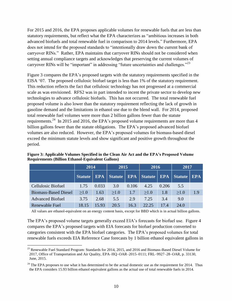
Figure 3 compares the EPA’s proposed targets with the statutory requirements specified in the
EISA ‘07. The proposed cellulosic biofuel target is less than 1% of the statutory requirement.
This reduction reflects the fact that cellulosic technology has not progressed at a commercial
scale as was envisioned. RFS2 was in part intended to incent the private sector to develop new
technologies to advance cellulosic biofuels. This has not occurred. The total renewable fuel
proposed volume is also lower than the statutory requirement reflecting the lack of growth in
gasoline demand and the limitations in ethanol use due to the blend wall. For 2014, proposed
total renewable fuel volumes were more than 2 billion gallons fewer than the statute
requirements.24
In 2015 and 2016, the EPA’s proposed volume requirements are more than 4
billion gallons fewer than the statute obligations. The EPA’s proposed advanced biofuel
volumes are also reduced. However, the EPA’s proposed volumes for biomass-based diesel
exceed the minimum statute levels and show significant and positive growth throughout the
period.
Figure 3: Applicable Volumes Specified in the Clean Air Act and the EPA’s Proposed Volume
Requirements (Billion Ethanol-Equivalent Gallons)
2014 2015 2016 2017
Statute EPA Statute EPA Statute EPA Statute EPA
Cellulosic Biofuel 1.75 0.033 3.0 0.106 4.25 0.206 5.5
Biomass-Based Diesel ≥1.0 1.63 ≥1.0 1.7 ≥1.0 1.8 ≥1.0 1.9
Advanced Biofuel 3.75 2.68 5.5 2.9 7.25 3.4 9.0
Renewable Fuel 18.15 15.93 20.5 16.3 22.25 17.4 24.0
All values are ethanol-equivalent on an energy content basis, except for BBD which is in actual billion gallons.
The EPA’s proposed volume targets generally exceed EIA’s forecasts for biofuel use. Figure 4
compares the EPA’s proposed targets with EIA forecasts for biofuel production converted to
categories consistent with the EPA biofuel categories. The EPA’s proposed volumes for total
renewable fuels exceeds EIA Reference Case forecasts by 1 billion ethanol equivalent gallons in
23
Renewable Fuel Standard Program: Standards for 2014, 2015, and 2016 and Biomass-Based Diesel Volume for
2017, Office of Transportation and Air Quality, EPA–HQ–OAR–2015–0111; FRL–9927–28–OAR, p. 33130,
June, 2015.
24 The EPA proposes to use what it has determined to be the actual domestic use as the requirement for 2014. Thus
the EPA considers 15.93 billion ethanol equivalent gallons as the actual use of total renewable fuels in 2014.

11
2015 and 2.1 billion ethanol equivalent gallons in 2016. The EPA’s proposed volumes for total
renewable fuels exceed EIA High Oil Price Case forecasts by 0.1 billion ethanol equivalent
gallons in 2015 and 0.9 ethanol equivalent gallons in 2016. The EPA’s cellulosic biofuel
volumes are roughly twice those forecasted by EIA. With biomass-based diesel for the years
2015 and 2016, the EPA’s proposed volumes exceed forecasted volumes in the EIA’s AEO
reference case but are less than volumes in the EIA’s High Oil Price case. In 2017, the EIA
forecasts in both cases exceed the EPA’s proposed volumes for biomass-based diesel.
Figure 4: Comparison of EIA forecasted Biofuel Volumes and EPA’s Proposed Volume
Requirements (Billion Ethanol-Equivalent Gallons)
EPA
Proposed
Requirement
AEO
Reference AEO High Oil Price
2015
Cellulosic Biofuel 0.106 0.043 0.041
Biomass-Based Diesel (BBD) 1.70 1.60 1.89
Advanced Biofuel 2.90 2.46 2.88
Renewable Fuel 16.3 15.3 16.2
2016
Cellulosic Biofuel 0.206 0.097 0.093
Biomass-Based Diesel (BBD) 1.80 1.65 2.03
Advanced Biofuel 3.40 2.60 3.15
Renewable Fuel 17.4 15.3 16.5
2017
Biomass-Based Diesel (BBD) 1.90 2.16 2.16
EIA does not report sugar ethanol imports. All values are ethanol-equivalent on an energy content basis, except
for BBD which is in actual billion gallons.
12
IV. DESCRIPTION OF THE MODELS
A. Transportation Fuel Model
The transportation fuel model is a recursive partial-equilibrium model designed to estimate the
amount of fuel produced for and consumed by the transportation sector. The model maximizes
the sum of producers’ surplus (a value to producers from producing fuels) and consumers’
surplus (a measure of household value from fuel consumption) subject to meeting the RFS2
program fuel requirements and satisfying the transportation sector’s demand for fuel while not
violating any transportation sector infrastructure constraints such as the blend wall, blend limit
for biodiesel, and RFS2’s RVOs.
The model is calibrated in 2015 and 2016 to the EIA’s Short-Term Energy Outlook (STEO) for
May 2015 and to the AEO2015 Reference forecast for 2017 through 2022, with a few minor
adjustments to the consumption of some biofuels to reduce the EIA forecasted values that occur
because of the existence of the EIA assuming the presence of an RFS policy.
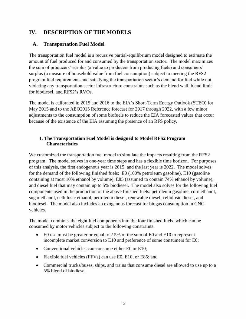
1. The Transportation Fuel Model is designed to Model RFS2 Program
Characteristics
We customized the transportation fuel model to simulate the impacts resulting from the RFS2
program. The model solves in one-year time steps and has a flexible time horizon. For purposes
of this analysis, the first endogenous year is 2015, and the last year is 2022. The model solves
for the demand of the following finished fuels: E0 (100% petroleum gasoline), E10 (gasoline
containing at most 10% ethanol by volume), E85 (assumed to contain 74% ethanol by volume),
and diesel fuel that may contain up to 5% biodiesel. The model also solves for the following fuel
components used in the production of the above finished fuels: petroleum gasoline, corn ethanol,
sugar ethanol, cellulosic ethanol, petroleum diesel, renewable diesel, cellulosic diesel, and
biodiesel. The model also includes an exogenous forecast for biogas consumption in CNG
vehicles.
The model combines the eight fuel components into the four finished fuels, which can be
consumed by motor vehicles subject to the following constraints:
E0 use must be greater or equal to 2.5% of the sum of E0 and E10 to represent
incomplete market conversion to E10 and preference of some consumers for E0;
Conventional vehicles can consume either E0 or E10;
Flexible fuel vehicles (FFVs) can use E0, E10, or E85; and
Commercial trucks/buses, ships, and trains that consume diesel are allowed to use up to a
5% blend of biodiesel.

13
2. RFS Constraints:
The model accounts for the minimum annual volume of biofuel sales required under the RFS2
scenario considered by including constraints on three types of biofuels:
Biomass-based diesel;
Advanced biofuel (includes cellulosic biofuels, biomass-based diesel, and sugar ethanol);
and
Renewable fuel (includes all above biofuel, corn ethanol, and imported renewable diesel).
For this analysis, we assume that cellulosic biofuels will continue to be commercially available
only in very limited quantities, and as a result, the EPA would continue to grant a cellulosic
waiver. This assumption avoids the debate about the economic and technical feasibility of
producing cellulosic fuels25
because this analysis assumes ample supplies of corn and sugar
ethanol to meet the RFS2 mandates. As a result, there is no need for cellulosic ethanol to meet
the non-cellulosic RFS2 targets.
3. Other Model Elements
As discussed in detail in Appendix B, the fuel supply curves capture all pertinent technological
issues (penetration rate, availability, and cost) for the different fuels. Similarly, the fuel demand
curves capture the loss in utility from having to reduce travel and also the loss in welfare from
fuel scarcity.
The model also incorporates constraints on the feedstocks of the finished fuels and on the
finished fuels themselves. For the feedstocks, there are upper limits on the amount of biodiesel,
renewable diesel, biogas, sugar ethanol, and cellulosic ethanol that can make it into the diesel or
gasoline pools. For these feedstocks there are quantity limits as well as limits as to how much
ethanol can be blended with petroleum gasoline and how much biodiesel can be blended with
petroleum diesel. The blend wall for gasoline is set at 10% and the blend limit for diesel is set at
5%.
Furthermore, there are limits on the availability of various finished fuels to account for both
consumer acceptance and infrastructure issues. The sales of E0 and E85 are limited based on
these issues. E0 must comprise at least 2.5% of the sum of E0 and E10; whereas the model
places an upper limit on the amount of E85 that can be consumed in each year.
25
There is a secondary effect of assuming no measurable supplies of cellulosic biomass. Assuming no significant
amount of cellulosic biomass production necessitates the production of additional amounts of biodiesel and sugar-
based ethanol to meet the advanced biofuel requirement, and this affects costs.

14
B. NewERA Macroeconomic Model
The NewERA macroeconomic model used for the current study is a static computable general
equilibrium model of the United States. Compared to a forward-looking dynamic model that
assumes perfect foresight with more certainty about the policy trend in the long term, the static
model is well suited for the policy with the great uncertainty like the current RFS policy as
exhibited by the EPA’s delay in setting the 2014 and 2015 standards. The model simulates all
economic interactions in the U.S. economy, including those among industry, households, and the
government. The macroeconomic and energy forecasts that are used to project the benchmark
year going forward are calibrated to AEO2015 Reference case produced by the EIA. Because
the model is calibrated to an internally-consistent energy forecast, the use of the model is
particularly well suited to analyze economic and energy policies and environmental regulations.
For this study, the NewERA model runs from 2015 to 2022 (or the last year in which the bottom-
up transportation model finds a feasible solution) in one-year increments. The model includes
five energy and seven non-energy sectors: energy sectors include crude oil, oil refining, natural
gas extraction and distribution, coal, and electricity; the non-energy sectors include agriculture,
commercial transportation (excluding trucking), energy intensive sectors, manufacturing, motor
vehicle production, services, and trucking.
The macroeconomic model incorporates all production sectors and final demands of the
economy and is linked through terms of trade. The effects of policies are transmitted throughout
the economy as all sectors and agents in the economy respond until the economy reaches
equilibrium. The ability of the model to track these effects and substitution possibilities across
sectors makes it a unique tool for analyzing policies such as those involving energy and
environmental regulations. These general equilibrium substitution effects, however, are not fully
captured in a partial-equilibrium framework or within an input-output modeling framework. The
smooth production and consumption functions employed in this general-equilibrium model
enable gradual substitution of inputs in response to relative price changes thus avoiding “all-or-
nothing” solutions.
Business investment decisions are informed by the current period policies and market forces.
The myopic characteristic of the static model determines the optimal consumption and
investment based on only the relative price changes in the current period thus agents have no
expectation for the future. The alternative approach on savings and investment decisions is to
assume the agents in the model have perfect foresight over the horizon. That is, to anticipate
what will happen in the future can change the consumption-investment decision today. Though
both approaches have their limitations, the former approach better reflects market expectations
and responses to the RFS2 policy given all the uncertainty about future targets, the time lags in
defining future targets, and the limited horizon for which future targets have been defined.
Consumers in the model are represented by a single regional representative household. The
representative household derives utility from both consumption of goods and services,

15
transportation services, and leisure. The model also represents federal and regional/state level
governments. The government collects federal and state taxes to support its expenditures.
We balance the international trade account in the NewERA model by constraining changes in the
current account deficit over the model horizon. The condition is that the net present value of the
foreign indebtedness over the model horizon remains at the benchmark year level. This prevents
distortions in economic effects that would result from perpetual increase in borrowing, but does
not overly constrain the model by requiring current account balance in each year.
The NewERA model is based on a unique set of databases constructed by combining economic
data from the IMPLAN 2008 (MIG Inc. 2010) database and energy data from the Energy
Information Administration (EIA’s) Annual Energy Outlook 2015 (AEO 2015). The IMPLAN
2008 database provides Social Accounting Matrices (SAMs) for all states for the year 2008.
These matrices have inter-industry goods and services transaction data; we rebuild the SAM and
merge the economic data with energy supply, demand, and prices consistent with AEO2015 from
EIA.
The NewERA model outputs include demand and supply of all goods and services, prices of all
commodities, and terms of trade effects (including changes in imports and exports). The model
outputs also include gross regional product, consumption, investment, disposable income and
changes in income from labor, capital, and resources.
More details of the model structure are presented in Appendix B.
C. Model Integration
The economic impacts of the RFS2 program were determined using the following methodology:
Using the transportation fuel model, the baseline and statute scenarios were run to determine
the effect on fuel prices resulting from the RFS2 requirements for increased use of biofuels.
Using the NewERA macroeconomic model, the resulting changes in fuel prices were
translated into taxes (or subsidies) on gasoline and diesel that yield the same fuel price
changes as seen in the transportation fuel model.
To ensure consistency between the transportation fuel model and the NewERA
macroeconomic model, we also calibrated the macroeconomic model in terms of relevant
elasticities such that for a given scenario, the macro model experiences the same quantity and
price impacts in the transportation sectors as in the transportation fuel model.
D. Analytical Methodology
The scenario was run using NERA’s transportation fuel model, which allowed us to simulate the
dynamics of RFS2 compliance and the use of surplus RIN carryovers, and the methodology that

16
the EPA uses each year to determine the minimum percentages of the different categories of
biofuels delineated in the RFS2 standard that fuel suppliers must use.
The transportation fuel model determined the impact of the RFS2 mandate on the quantities of
finished gasoline (E0 and E10), E85, and diesel consumed in the transportation sector. In
addition, the model calculated volumes of individual biofuels blended in the finished gasoline
(corn ethanol, sugar ethanol, and cellulosic ethanol) and diesel (biodiesel and renewable diesel).
The NewERA macroeconomic model then determined the impact on the U.S. economy of
meeting the RFS2 mandate given the price and volume responses to the modeled RFS program
forecasted by the bottom-up transportation sector model. The results are expressed in terms of
well-known economic parameters: changes in consumer purchasing power, GDP, and labor
earnings.
Implementation of the RFS2 may create a dynamic in which higher costs in the current year lead
to lower demand, which in turn lead to higher costs in the next year and so on.
NERA’s transportation fuel model represents this process by solving in a recursive dynamic
fashion. That is, the model solves for the mix of feedstocks and finished fuels that minimizes the
cost of compliance with RFS2 for the current year, through the use and value of surplus RINs
that were carried forward and the carrying forward of RINs for the following year. Therefore,
the years are linked through the RINs.
RIN carryover in this report represents how surplus RINs can be carried over from one
compliance period to the next by an obligated party. We assume that as of the beginning of
January 2015 the D6 RIN carryover bank was 1.8 billion gallons.26
We refer to these RINs as
the initial inventory of RINs available for compliance. After defining the RINs available at the
beginning of 2015 and calibrating the model’s supply and demand curves to the AEO’s
forecasted 2015 values, the model was solved with the RFS2 constraints and other infrastructure
constraints for the year 2015.
The RINs available at the end of 2015, or the number of RINs carried forward to 2016, equals
the RINs available at the beginning of 2015 (1.8 billion gallons) plus the difference between the
number of RINs generated and the number of RINs submitted for compliance during 2015
If any of the RFS2 or infrastructure constraints bind, then the average fuel price may rise to
cause a switch in fuel consumption patterns which results in an increase of the percentage of
renewable fuel sales to the level required by the RFS2 constraint. An increase in average fuel
prices would cause a drop in the equilibrium level of fuel consumption from the EIA’s forecast.
The value of the elasticity of demand has a significant effect on the relationship between the
increase in fuel price and decline in fuel demand. The more elastic the demand curve, the less
26
Renewable Fuel Standard Program: Standards for 2014, 2015, and 2016 and Biomass-Based Diesel Volume for
2017, Office of Transportation and Air Quality, EPA–HQ–OAR–2015–0111; FRL–9927–28–OAR, p. 33130,
June, 2015.

17
prices need to move to induce consumers to reduce their demand and thus the easier and less
costly it is to meet the RFS2 targets. As the absolute value of the elasticity of demand declines,
demand becomes more inelastic and the cost of compliance increases.
Once finished with 2015, the model then solves for 2016. However, instead of using the EIA’s
forecast for 2016 energy consumption, the values to which the model calibrates its energy
consumption are adjusted based on the model’s 2015 solution values for energy consumption.
Assuming that the RFS2 constraint binds for 2015, the forecasted fuel sales volumes will differ
in 2015 from that of the EIA’s forecast.
To be conservative regarding the costs of the RFS2 mandate, we allow surplus RINs to be
exhausted over the model horizon. Retaining RINs for later years would raise program costs in
the near term. This is because the transportation sector would need to consume higher
percentage levels of biofuels in the near term instead of relying on the RINs generated in prior
years to assist the sector in complying with RFS2. Allowing the RINs to be consumed in the
near term (e.g., by 2022) rather than retaining RINs after 2022 allows obligated parties to meet
the mandates with lower volumes of renewable fuels and hence reduces the burden of the policy.
E. Model Parameters
1. Fuel Prices
All fuel prices are national, annual averages over multiple grades of fuel. Our baseline prices for
finished products (gasoline and diesel) are the same as those forecast in the AEO2015 Reference
Case. The NERA baseline prices for individual types of biofuels were developed using a variety
of sources and are expressed relative to petroleum gasoline or diesel prices. These relative prices
are shown in Figure 5, and the logic and sources upon which these relative prices are based are
described below.27
27
The gasoline, diesel, and corn ethanol prices are taken from the AEO 2015 Reference case.

18
Figure 5: Baseline Fuel Price Ratios for Blended Gasoline and Diesels (Ratio on a GGE28
Basis of
Biofuel to Conventional Fuel)29
2015 2016 2017 2018 2019 2020 2021 2022
Corn Ethanol 1.38 1.19 1.47 1.44 1.42 1.34 1.34 1.31
Sugarcane Ethanol 1.59 1.37 1.69 1.65 1.63 1.54 1.54 1.51
Cellulosic Ethanol 2.23 1.92 2.36 2.32 2.28 2.16 2.17 2.12
Soy-Based Biodiesel 1.92 1.69 1.65 1.65 1.65 1.62 1.60 1.58
Renewable Diesel 1.93 1.69 1.65 1.65 1.65 1.62 1.60 1.58
Source: EIA’s AEO2015, EIA, California Energy Commission, and NERA analysis.
Ethanol:
Ratio of corn ethanol to gasoline is from the AEO2015 Reference Case, Table A12.
Sugar Ethanol: Ratio of sugar ethanol prices to gasoline prices taken from California
Energy Commission statistics.30
Cellulosic Ethanol: Ratio of cellulosic ethanol prices to gasoline prices based on EIA’s
cost build up.31
However, the future cost of cellulosic ethanol is uncertain.
Soy-Based Biodiesel: Ratio of soy-based biodiesel to petroleum diesel prices based upon EIA’s
cost buildup modified for current soy bean prices.32
Renewable Diesel: Ratio of renewable diesel to petroleum diesel prices based upon EIA’s Cost
buildup modified for current feedstock prices.33
2. Supply Elasticities
In addition, supply elasticities were derived by using fuel price and fuel supply information from
EIA’s AEO 2011 and AEO 2015 Reference and High Oil Price Cases. These cases provided
time series for the prices and quantities of the different fuels. The price elasticity of supply for
each fuel is derived by dividing the percentage change in quantity of fuel demanded by the
percentage change in fuel price. The percentage change in quantity and price are computed by
comparing the difference between the fuel consumed and the price of fuel, respectively, in the
AEO High Oil Price and Reference Cases. The elasticity of supply varies slightly from year to
year, but on average, the elasticity of supply is about 0.4 for corn ethanol and 2.0 for soy-based
biodiesel. Because sugar ethanol exported to the U.S. is a small percentage of the total sugar
ethanol produced, we assume a high supply elasticity of 4 for this fuel. The elasticity for
28
Gasoline gallon equivalent basis; fuels GGE are adjusted by relative heating value to petroleum gasoline. 29
All price ratios are national, annual averages over multiple grades of fuel. For gasoline, the grades include regular
unleaded, 89 octane unleaded, and premium unleaded. 30
2011 Integrated Energy Policy Report, California Energy Commission, February, 2012. 31
Assumptions to AEO2014, Table 11.9. 32
Assumptions to AEO2014, Table 11.9. 33
Assumptions to AEO2014, Table 11.9.

19
petroleum fuels is 0.8.34
To account for the ability of the market to respond more over time, the
supply elasticities increase by 5% per year.
3. Demand Elasticities
The model has a demand curve for each finished fuel – E0, E10, E85, and diesel. The functional
form of these curves is identical to that of the fuel supply curves. For the demand curves, the
elasticity is the fuel’s own-price elasticity of demand. The E10 and diesel demand curves’
elasticity for 2015 is set equal to Dahl’s estimate for short-term elasticity of -0.1.35
To allow for
the trade-off between E10 and E0 for conventional vehicles and E10 and E85 for FFVs, we
assume a demand elasticity of -0.5 for E0 and E85. To account for the ability of the market to
respond more over time, the supply elasticities increase by 10% per year.
4. E85
The Fuels Institute undertook a study of E85.36
They extensively reviewed historical sales.
From this analysis, they developed forecasts of future E85 sales based on assumptions about the
penetration of E85 stations and the throughput at stations that sell E85. We based our estimates
of potentially available E85 solely upon Fuels Institute’s Top Quartile Scenario. This scenario
assumes every E85 retail station has the ability to match the performance of the Top Quartile of
stores reported in the Fuels Institute sample. These stores sold on average 364 gallons of E85 per
day. The model forecasts potential daily E85 volume of 619 gallons per store by 2023. Applying
this per store E85 daily sales forecast to the total number of E85 stores, the model forecasts that
by 2023 such a market could generate 2.2 billion gallons of E85 sales.37
Figure 6 reports the Fuels Institute’s Top Quartile forecast and the EIA’s AEO 2015 Reference
Case forecast. Comparing the two forecasts shows that the Top Quartile forecast is extremely
optimistic compared to the EIA’s forecast. Using the Top Quartile forecast does not fully
account for consumer reluctance of consuming E85, which stems from the lower fuel economy
and limited range of E85. Therefore, the Top Quartile forecast serves as an optimistic upper
level on E85 sales.
34
Paltsev, Sergey, John M. Reilly, Henry D. Jacoby, Richard S. Eckaus, James McFarland, Marcus Sarofim,
Malcolm Asadoorian, and Mustafa Babiker, “The MIT Emissions and Prediction and Policy Analysis (EPPA).
Model Version 4,” August, 2005. 35
Dahl, C.A., “A survey of energy demand elasticities for the developing world,” Journal of Energy and
Development 18(I), 1—48, 1994. 36
“E85 – A Market Performance and Forecast, Fuels Institute,” 2014.
37 “E85 – A Market Performance and Forecast, Fuels Institute,” p. 34, 2014.

20
Figure 6: Fuels Institute’s Top Quartile and EIA’s E85 Sales Forecasts (Billion Gallons)
2015 2016 2017 2018 2019 2020 2021 2022
Fuels Institute 0.40 0.51 0.65 0.83 1.06 1.35 1.72 2.20
EIA 0.34 0.37 0.22 0.22 0.27 0.29 0.39 0.64
Source: EIA’s AEO 2015, Fuels Institute.
5. Upper Bounds on Supply of Various Biofuels
The model incorporates production or consumption limits on the following biofuels: Cellulosic
Biofuel, Sugar Ethanol, Biogas, Biodiesel, and Renewable Diesel. The maximum supply of
biofuels is shown in Figure 7, and the logic and sources upon which these levels were derived is
described below.
Figure 7: Maximum level of biofuels (Billion Gallons)
Ethanol Diesel
Cellulosic Sugar Biogas Bio Renewable
2015 0.04 0.68 0.13 1.90 0.30
2016 0.10 0.75 0.31 2.03 0.30
2017 0.14 0.82 0.49 2.16 0.30
2018 0.16 0.91 0.49 2.29 0.30
2019 0.17 1.00 0.49 2.47 0.33
2020 0.17 1.10 0.49 2.67 0.43
2021 0.17 1.20 0.49 2.87 0.54
2022 0.17 1.33 0.49 3.07 0.68
As discussed earlier, the EPA can waive the RFS2 requirement, in whole or in part, if there is an
inadequate domestic supply. With respect to the cellulosic biofuels mandate, there is an
established track record by the EPA of substantially reducing the cellulosic biofuel requirement
because of the lack of commercially-available production. In 2010 and 2011, there were no
cellulosic biofuel RINs generated. For 2012, the EPA has reduced the requirement for cellulosic
biofuels to less than 10 million gallons from the 500 million gallons required under RFS2.
As a result of the lack of progress in developing commercially-available supplies of cellulosic
biomass and the technical and economic hurdles that remain with the production of cellulosic
ethanol, and the time required to build and put into service biomass-to-liquids facilities, we
concluded that it was unlikely that cellulosic biofuels will be used in any appreciable quantities
during our forecast horizon.

21
The maximum supply of cellulosic ethanol was set equal to the maximum of the consumption of
cellulosic ethanol in the AEO’s 2015 Reference and High Oil Price case. The maximum supply
of cellulosic ethanol is 0.03, 0.12, and 0.14 Billion gallons for 2015, 2016, and 2017,
respectively. AEO 2015 High Oil Price case forecasts these volumes for these years.
The maximum amount of sugar ethanol was set to 680 million gallons, the quantity that the U.S.
imported in 2006. This is the highest volume of Brazilian ethanol that the U.S. ever imported,
and imports in recent years have been considerably lower. In 2014, imports were only 64 million
gallons. Production of sugarcane ethanol in Brazil has increased in recent years, but demand for
ethanol in Brazil has also increased. This maximum is increased by 10% for each year from 2016
to 2022.
In the NPRM, the EPA provides values for CNG/LNG production in new facilities and in
existing facilities in 2015 and 2016. We set the maximum limits on biogas to the sum of the
EPA’s high end estimates for production of CNG/LNG in new and existing facilities for each
year. We use the annual growth rate of biogas production that the EPA determines for 2015 to
2016 to calculate biogas production limits in 2017 and then maintain the upper limit of biogas at
the 2017 level through 2022.
The NPRM estimates the consumption of 1.69 billion gallons of total biomass-based diesel in
2014. The model’s maximum allowable amount of biomass-based diesel consumption from
2015 to 2022 is computed by adding 0.2 billion gallons per year to the 2014 value. Renewable
diesel capacity is set equal to the maximum of the EIA’s AEO 2015 Reference Case38
consumption of renewable diesel and the amount of renewable diesel supplied to the market in
2014 according to the EPA’s NPRM. For 2015, the level of renewable diesel consumption in the
AEO 2015 Reference Case exceeds the corresponding value in the High Oil Price Case. The
maximum biodiesel capacity is assumed to be 10% greater than the difference between
maximum capacities of the total biomass-based diesel and renewable diesel. This forecast for
maximum potential production exceeds the EIA’s AEO 2015 High Oil Price Case consumption
level.
6. Other Fuel Constraints and Assumptions
The Statute Scenario imposed both the gasoline blend wall (no more than 10% ethanol) as well
as the biodiesel blend limit (no more than 5% biodiesel). We allowed petroleum gasoline either
to be blended with ethanol to make E10 or E85, or to be sold as neat gasoline (E0). A review of
EIA data from May 2008 through May 2015 showed that E0 reached a low of about 2.5% in the
spring/summer of 2012. The more gasoline that is used to produce E0 means that there is less to
be blended with ethanol, and hence the more difficult it would be to comply with RFS2. To be
conservative in our assessment of the compliance costs of RFS2, we assumed the share of the E0
38
The EIA’s 2015 AEO Reference case forecasts greater amounts of renewable diesel than its High Oil Price case.
22
and E10 gasoline pool that is E0 can drop no lower than 2.5%. This is consistent with data
generated by EIA.39
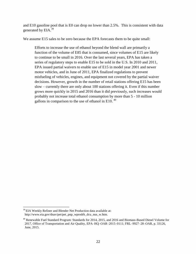
We assume E15 sales to be zero because the EPA forecasts them to be quite small:
Efforts to increase the use of ethanol beyond the blend wall are primarily a
function of the volume of E85 that is consumed, since volumes of E15 are likely
to continue to be small in 2016. Over the last several years, EPA has taken a
series of regulatory steps to enable E15 to be sold in the U.S. In 2010 and 2011,
EPA issued partial waivers to enable use of E15 in model year 2001 and newer
motor vehicles, and in June of 2011, EPA finalized regulations to prevent
misfueling of vehicles, engines, and equipment not covered by the partial waiver
decisions. However, growth in the number of retail stations offering E15 has been
slow – currently there are only about 100 stations offering it. Even if this number
grows more quickly in 2015 and 2016 than it did previously, such increases would
probably not increase total ethanol consumption by more than 5 - 10 million
gallons in comparison to the use of ethanol in E10. 40
39
EIA Weekly Refiner and Blender Net Production data available at:
http://www.eia.gov/dnav/pet/pet_pnp_wprodrb_dcu_nus_w.htm.
40 Renewable Fuel Standard Program: Standards for 2014, 2015, and 2016 and Biomass-Based Diesel Volume for
2017, Office of Transportation and Air Quality, EPA–HQ–OAR–2015–0111; FRL–9927–28–OAR, p. 33126,
June, 2015.

23
V. RESULTS
A. Study Results
As shown in Figure 8, when the required volume of total renewable fuel is equal to the EISA ’07
statute requirement,the Statute Scenario exhibits a decrease in gasoline and diesel demand vs.
EIA and outrageously high consumer costs that are evident immediately, i.e, in 2015. The 2015
statutory requirement would require about 30%41
more RINs to be generated than were generated
in 2014. In order to achieve the associated required blending percentage for obligated parties
with the supply of available RINs requires about a 30% reduction in gasoline and diesel volumes
from expected demand in 2015. To achieve this reduction in gasoline and diesel demand
requires that costs increase by roughly $90 and $100 per gallon more than today’s costs,
respectively.
Figure 8: 2015 Gasoline and Diesel Results in Statute Scenario
Fuel Demand
(Billion Gallons)
Cost to Consumer
($/Gallon)
Gasoline 93 $92
Diesel 40 $103
Source: NERA analysis.
The price increases in gasoline and diesel are accompanied by a reduction in demand for the
transportation fuels. Since the transportation sector is interconnected with other sectors in a way
that the transportation services are consumed by other sectors, the fuel cost increase creates the
spillover effects that ripple through the economy. Higher diesel fuel costs increase the cost to
move raw materials and finished goods around the country, thus eventually making everything
that directly or indirectly depends on transportation services more costly. Likewise the higher
gasoline prices leave consumers with less disposable income. As a result of these impacts,
consumption of goods and services declines. All of these impacts lead to severe economic harm.
B. The Dilemma with RFS2
There is a fundamental problem with the RFS2 mandate: the blending percentage standard for
total renewable fuel, at statutory volumes exceeds the maximum feasible level of renewable fuel
that can be contained on average in a gallon of transportation fuel given the technological,
market, and infrastructure constraints in the economy. For 2015, this percentage is calculated at
11.6%.42
This results in a market disruption as it is impossible to achieve the RFS2 biofuel
41
EPA proposes 15.9 billion RINs for 2014. The statute requires 20.5 billion RINs in 2015.
42 Source: NERA assumptions and analysis. The ratio of the RIN gallons to the sum of gallons in the diesel and
gasoline pools including E85 less the statute level RIN gallons for total renewable fuels.
24
volume targets because E10 has a percentage value of 11.1% and B5 has a percentage value of
8.1%.
This issue of exceeding the maximum feasible level will only be exacerbated by the forecasted
declining consumption of gasoline because of the tighter CAFE standards, which will lead to
improved fuel economy and less gasoline consumption.
C. Macroeconomic Impacts
The price increases in gasoline and diesel are accompanied by a reduction in demand for the
transportation fuels. Since the transportation sector is interconnected with other sectors in a way
that the transportation services are consumed by other sectors, the fuel cost increase creates the
spillover effects that ripple through the economy. Higher diesel fuel costs increase the cost to
move raw materials and finished goods around the country, thus eventually making everything
that directly or indirectly depends on transportation services more costly. As a result,
consumption of goods and services declines.
During the model horizon, labor earnings decrease. This decline results from two competing
effects on the production side – a substitution and an output effect. The substitution effect
occurs as the increase in the cost of transportation services leads other sectors to substitute away
from transportation services toward value added inputs like labor and capital to help reduce the
total cost of production. The effect on output occurs where the cost increase in transportation
service pushes up the output price which leads to a reduction in the level of production and lower
demand for all inputs. When the output effect outweighs the substitution effect, the demand for
labor falls, leading to a lower wage rate and lower labor earnings.
Consumption falls by an even greater amount. In addition to the negative impact of higher costs
for finished goods and services caused by rising diesel and gasoline costs, consumers are left
with fewer dollars to spend on other goods and services resulting in lower consumption. Lower
consumption translates into less need for the production of other goods and services that
consumers would have purchased in the absence of RFS2.
The combined effect of less disposable income and the higher cost for finished goods and
services means that consumption declines even further.

25
VI. CONCLUSIONS
Based upon NERA’s modeling of the transportation sector and the overall economy for
implementing the RFS2 biofuel volume requirements, NERA concludes:
In 2015 and beyond, it is not feasible to achieve the statute volumes of total renewable
fuel required under EISA ‘07. The current level of gasoline demand, the blend wall
limiting the share of ethanol that can be blended into the gasoline pool, and the lack of
non-ethanol biofuels limit the market potential for total renewable biofuels. Similarly the
current market potential for higher ethanol content gasoline like E85 and E15 is too small
to have an immediate impact on the amount of ethanol that the gasoline market can
absorb.
Only by the EPA invoking its two different waiver authorities43
to issue a waiver for
cellulosic ethanol and the same deduction for the total renewable biofuels and advanced
biofuel volumes requirements as well as a general waiver for both advanced biofuels and
total renewable fuels would allow the RFS2 to be feasible.
NERA’s conclusion that it is infeasible to achieve the statute volumes for total renewable
fuels in 2015 and beyond is consistent with NERA’s findings from its 2012 study, which
also found that if the EPA retained the EISA ’07 statute volumes, severe economic harm
would result in the 2015 to 2016 time frame. Infeasibility has not occurred yet because
EPA has recognized the blend wall and is proposing volumes below the statute levels.
Economic harm: When the required biofuel volume standards are too severe, as with the statute
scenario, the market becomes disrupted because there are an insufficient number of RINs to
allow compliance. “Forcing” additional volumes of biofuels into the market beyond those that
would be “absorbed” by the market based on economics alone at the levels required by the
statute scenario will result in severe economic harm.
43
The cellulosic ethanol waiver allows EPA to reduce applicable volumes for cellulosic biofuels and apply the same
reduction to the total renewable biofuels and advanced biofuel volumes requirements. The general waiver allows
EPA to reduce volumes for any renewable fuel if there is inadequate supply.

26
APPENDIX A. DETAILED MODEL DESCRIPTION
This analysis used the linked system of NERA’s proprietary bottom-up transportation fuel model
and its NewERA macroeconomic model. This section describes these two models.
A. Transportation Fuel Model
The transportation fuel model is a partial equilibrium model designed to estimate the amount of
fuel produced for and consumed by the transportation sector with and without the RFS2 policy in
place. The model maximizes the sum of consumers’ and producers’ surplus subject to meeting
the RFS2 program fuel requirements and satisfying the transportation sector’s demand for fuel
while not violating any transportation sector infrastructure constraints.
1. Fuel Supply Curves
To address the changes in fuel production from the baseline, we use separate supply curves for
each fuel. The elasticity of the supply dictates how the prices of fuels change with changes in
production.
The own price elasticity for each fuel is derived by dividing the percentage change in quantity of
fuel demanded by the percentage change in fuel price. The percentage change in quantity and
price are computed by comparing the difference between the fuels consumed and price of fuel,
respectively, in the AEO high oil price and reference cases. The elasticity of supply varies a bit
from year to year, but on average, the elasticity of supply is about 0.4 for corn ethanol and 1.2
for biodiesel. The elasticity for petroleum fuels was is 0.8.44
Because sugar ethanol for the U.S.
is a small percentage of the total sugar ethanol produced, we assume a high supply elasticity of 4
for this fuel. To account for the ability of the market to respond more over time, the supply
elasticities increase by 5% per year.
2. Demand Curves
The model has a demand curve for each final fuel – E0, E10, E85, and diesel. The functional
form of these curves is identical to that of the fuel supply curves. For the demand curves, the
elasticity is the fuel’s own price elasticity of demand. The E10 and diesel demand curves’ initial
elasticity equals that of Dahl’s estimate for short-term elasticity of -0.1.45
To allow for the trade-
off between E10 and E0 for conventional vehicles and E10 and E85 for FFVs, we assume a
demand elasticity of -0.5 for E0 and E85. To account for the ability of the market to respond
more over time, the supply elasticities increase by 10% per year.
44
Paltsev, Sergey, John M. Reilly, Henry D. Jacoby, Richard S. Eckaus, James McFarland, Marcus Sarofim,
Malcolm Asadoorian, and Mustafa Babiker, “The MIT Emissions and Prediction and Policy Analysis (EPPA).
Model Version 4,” August, 2005. 45
Dahl, C.A., “A survey of energy demand elasticities for the developing world,” Journal of Energy and
Development 18(I), 1—48, 1994.

27
These curves are calibrated to the demand data. The EIA’s AEO 2015 Reference Case provides
the gasoline and diesel prices to which the demand curves’ initial prices are calibrated (Figure 9).
Figure 9: AEO 2015 Reference Case Fuel Prices (2013$/Gallon)
2015 2016 2017 2018 2019 2020 2021 2022
Gasoline 2.31 2.63 2.70 2.70 2.70 2.74 2.78 2.82
Diesel 2.66 2.96 3.00 3.02 3.06 3.11 3.16 3.24
Source: AEO 2015 Reference Case Table C5.
4. Transportation Fuel Model is Designed to Model RFS2 Program Characteristics
The transportation fuel model was customized to simulate the impacts resulting from the RFS2
program. The model solves in one-year time steps and has a flexible time horizon. The first
endogenous year is 2015. The model tracks the sale of the following fuels: E0 (100% petroleum
gasoline), E10 (gasoline containing at most 10% by volume ethanol), E85 (assumed to contain
74% ethanol by volume), and diesel (containing at most 5% biodiesel). The model also tracks
the use of the following fuel components in the production of the above finished fuels: petroleum
gasoline, corn ethanol, sugar ethanol, cellulosic ethanol, petroleum diesel, biodiesel, renewable
diesel, and biogas.
Biogas is assumed to be consumed by CNG vehicles. The model combines the remaining fuel
components into the four end-use fuels, which can be consumed by specific vehicle types:
Minimum E0 cannot drop below 2.5% of the sum of E0 and E10. The amount of E0
represents the incomplete market conversion to E10 and preference of some consumers
for E0;
Conventional vehicles can consume either E0 or E10;
FFVs can use E0, E10, or E85; and
Commercial trucks/buses, ships, and trains are allowed to use diesel, which has up to a
five percent mix of biodiesel (B5), where the denominator includes petroleum, bio-, and
renewable diesel.
5. RFS/RIN Constraints
The model includes three biofuel constraints to account for the minimum annual volume of
biofuel sales required under the RFS2 program:
Biomass based diesel;
Advanced biofuel (includes cellulosic biofuels, biomass-based diesel, and sugar ethanol);
and
Renewable fuel (includes advanced biofuel and corn ethanol).

28
For this analysis, we assume the EPA grants nearly a full waiver on cellulosic ethanol. The
RFS2 constraint for cellulosic ethanol in each year is set equal to the maximum amount that the
model assumes can be produced in that year. This assumption avoids the debate about the
economic and technical feasibility of producing cellulosic biofuel46
and is likely optimistic given
the current difficulty procuring cellulosic biofuel supplies. Since this analysis assumes ample
supplies of corn ethanol, sugar ethanol, and biomass based diesel to meet the RFS2 mandates,
there is no need for cellulosic ethanol to meet the non-cellulosic RFS2 targets.
Therefore, we model the following three RFS2 constraints, which are defined in the EPA’s Final
Rule for the Regulation of Fuels and Fuel Additives (see Figure 10).
Figure 10: EPA’s Formulas for the RFS2 Percentage Mandates47
46
We note that there is a second- or third-order effect of assuming no measurable cellulosic supplies. Assuming no
significant amount of cellulosic ethanol production necessitates additional amounts of biodiesel and sugar based
ethanol to meet the advanced biofuel requirement, and this affects costs and compliance. 47
Renewable Fuel Standard Program: Standards for 2014, 2015, and 2016 and Biomass-Based Diesel Volume for
2017, Office of Transportation and Air Quality, EPA–HQ–OAR–2015–0111; FRL–9927–28–OAR, p. 33146,
June, 2015.

29
The EPA’s proposed standards for 2015 and 2016 are provided below in Figure 11.
Figure 11: EPA’s Proposed Rule for RFS standards for 2015 and 201648
2015 2016
Cellulosic Biofuel 0.059% 0.114%
Biomass-Based Diesel 1.41% 1.49%
Advanced Biofuel 1.61% 1.88%
Renewable Fuel 9.04% 9.63%
Source: EPA.
6. Model Formulation
The following text describes the transportation fuel model – its objective function and constraints
- at a high-level.
Maximize: Consumer Surplus + Producer Surplus + Value of RIN Bank
Subject to: RFS2 advanced biofuel constraint (% requirement)
RFS2 biodiesel constraint (% requirement)
RFS2 total biofuel constraint (% requirement)
Blend wall constraint for E10 not to exceed 10% ethanol
Blend limit constraint for diesel not to exceed 5% biodiesel
Limit on E85 sales based on Fuels Institute Top Quartile Case
Lower bound on E0 sales as a fraction of E0 and E10 sales
Upper bound on biofuel production for cellulosic ethanol, sugar ethanol,
biogas, biodiesel, renewable diesel and total biomass based diesel
RIN bank(t) = RIN bank(t-1) + RIN Deposit(t) – RIN withdrawal(t) t = 2015, …, 2022
RIN bank cannot exceed 20% of biofuel sales…
Consumer Surplus = the area under the demand curve for each delivered fuel (e.g., E0,
E10, etc.)
Producer Surplus = the area under the supply curve for each fuel component (e.g., corn
ethanol, biodiesel, etc.)
The starting level of carryover D6 RINs at the beginning of 2015 equals 1.8 Billion RINs.
The supply curves capture the technological issues (penetration rate, availability, and cost) for
the different fuels. The demand curves for fuel capture the loss in utility from having to reduce
travel and also the loss in welfare from having to switch fuels. The RFS constraint is applied to
the Statutory Scenario. The limits for biofuels and E85 sales are reported in billions of gallons.
48
Renewable Fuel Standard Program: Standards for 2014, 2015, and 2016 and Biomass-Based Diesel Volume for
2017, Office of Transportation and Air Quality, EPA–HQ–OAR–2015–0111; FRL–9927–28–OAR, p. 33148,
June, 2015.

30
B. NewERA Macroeconomic Model
1. Overview of the NewERA Macroeconomic Model
The NewERA macro model is a forward-looking, dynamic, computable general equilibrium
model of the United States. The model simulates all economic interactions in the U.S. economy,
including those among industry, households, and the government. The economic interactions are
based on the IMPLAN49
2008 database for a benchmark year, which includes regional detail on
economic interactions among 440 different economic sectors. The macroeconomic and energy
forecasts that are used to project the benchmark year going forward are calibrated to the most
recent AEO 2014 produced by the Energy Information Administration (EIA). Because the model
is calibrated to an internally-consistent energy forecast, the use of the model is particularly well-
suited to analyze economic and energy policies and environmental regulations.
2. Model Data (IMPLAN and EIA)
The economic data is taken from the IMPLAN 2008 database, which includes balanced Social
Accounting Matrices for all states in 2008. These inter-industry matrices provide a snapshot of
the economy. Since the IMPLAN database contains only economic values, we benchmark
energy supply, demand, trade, and prices to EIA historical statistics to capture the physical
energy flows. The integration of the EIA energy quantities and prices into the IMPLAN
economic database results in a balanced energy-economy dataset.
Future economic growth is calibrated to macroeconomic GDP, energy supply, energy demand,
and energy price forecasts from the EIA AEO 2014. Labor productivity, labor growth, and
population forecasts from the U.S. Census Bureau are used to project labor endowments along
the baseline and ultimately employment by industry.
3. Brief Discussion of Model Structure
The theoretical construct behind the NewERA model is based on the circular flow of goods,
services, and payments in the economy (every economic transaction has a buyer and a seller
whereby goods/service go from a seller to a buyer and payment goes from the seller to the
buyer). As shown in Figure 12, the model includes households, businesses, government,
financial markets, and the rest of the world economy as they interact economically in the global
economy. Households provide labor and capital to businesses, taxes to the government, and
savings to financial markets, while also consuming goods and services and receiving government
subsidies. Businesses produce goods and services, pay taxes to the government and use labor
and capital. Businesses are both consumers and producers of capital for investment in the rest of
the economy. Within the circular flow, equilibrium is found whereby goods and services
49
IMPLAN produces unique set of national structural matrices. The structural matrices form the basis for the inter-
industry flows which we use to characterize the production, household, and government transactions, see
www.implan.com.

31
consumed is equal to those produced and investments are optimized for the long term. Thus,
supply is equal to demand in all markets.
The model assumes a perfect foresight, zero profit condition in production of goods and services,
no changes in monetary policy, and full employment within the U.S. economy.
Figure 12: Circular Flow of Income
a. Regional Aggregation
The standard NewERA macro model includes 11 regions: NYNE-New York and New England;
MAAC-Mid-Atlantic Coast; UPMW-Upper Mid-West; SEST-South East; FLST-Florida;
MSVL-Mississippi Valley; MAPP-Mid America; TXOL-Texas, Oklahoma, and Louisiana;
AZMT-Arizona and Mountain states; CALI-California; and PNWS-Pacific Northwest.50
The
aggregate model regions are built up from the 50 U.S. states’ and the District of Columbia’s
economic data. The model is flexible enough to create other regional specifications. The 11
NewERA regions and the States within each NewERA region are shown in the following figure.
50
Hawaii and Alaska are included in the PNWS region.
Households Firms
Factors of
Production
Foreign
Countries
Goods and
Services
United States
Factor
Payments
Taxes
ExportsImports
TaxesGovernment

32
For this Study we aggregate the 50 states into two regions: For this Study we aggregate the 50
states into one region: USA.
Figure 13: Standard NewERA Model’s Macroeconomic Regions
b. Sectoral Aggregation
The NewERA model includes 12 sectors: six energy sectors (coal, natural gas, crude oil,
electricity, and refined petroleum products) and seven non-energy sectors (services,
manufacturing, energy-intensive, agriculture, motor vehicle production, trucking, and
commercial transportation excluding trucking). We represent a single type of crude oil and
multiple refined petroleum products where oil use by sector is differentiated. These sectors are
aggregated up from the 440 IMPLAN sectors to 28 sectors, defined as the AEO 2014 sector in
Figure 14. These 28 sectors’ economic and energy data are consistent with IMPLAN and EIA,
respectively. For this study, we further aggregate these 28 production sectors into 12 production
sectors. The mapping of the sectors is shown below in Figure 14. The model has the flexibility
to represent sectors at any level of aggregation.

33
Figure 14: NewERA Sectoral Representation in Core Scenarios51
c. Production and Consumption Characterization
Behavior of households, industries, investment, and government is characterized by nested CES
production or utility functions. Under such a CES structure, inputs substitute against each other
in a nested form. The ease of substitutability is determined by the value of the elasticity of
substitution between the inputs. The greater the value of the substitution elasticity between the
inputs; the greater the possibility of tradeoffs.
The CES nesting structure defines how inputs to a production activity compete with each other.
In the generic production structure, intermediate inputs are aggregated in fixed proportion with a
composite of energy and value-added inputs. The energy input aggregates fossil and non-fossil
energy sources, and the value-added input combine capital and labor. Sectors with distinctive
51
We expand our default sectoral definition for the chemicals analysis to include ethane as an additional commodity
and three additional sectors representing chemicals subsectors. We describe these additions in detail in Chapter
VIII.
NewERA AEO
C C Household consumption G G Government consumption I I Investment demand
COL COL Coal GAS GAS Natural gas OIL OIL Refined Petroleum Products CRU CRU Crude oil ELE ELE Electricity
AGR AGR Agriculture TRN TRN Transportation TRK TRK Trucking M_V M_V Motor vehicle SRV SRV Services SRV DWE Dwellings
EIS PAP Paper and Pulp EIS CHM Chemicals EIS GLS Glass Industry EIS CMT Cement Industry EIS I_S Primary Metals EIS ALU Alumina and Aluminum
MAN CNS Construction MAN MIN Mining MAN FOO Food, Beverage and Tobacco Products MAN FAB Fabricated Metal Products MAN MAC Machinery MAN CMP Computer and Electronic Products MAN TRQ Transportation Equipment MAN ELQ Electrical Equip., Appliances, and Components MAN WOO Wood and furniture MAN PLA Plastics MAN OMA Other Manufacturing sectors
Final Demand
Energy Sectors
Non-Energy Sectors

34
production characteristics are represented with structures different from the generic form. For
alternative transportation fuels, such as ethanol and bio-diesel, inputs are demanded in fixed
proportion. The characterization of nonrenewable resource supply adds a fixed resource that is
calibrated to a declining resource base over time, so that it implies decreasing returns to scale.
This also implies rising marginal costs of production over time for exhaustible resources. The
detailed nesting structure of the households and production sectors, with assumed elasticity of
substitution parameters, is shown in figures below.
i. Households
Consumers are represented by a single representative household. The representative household
derives utility from both consumption of goods and services, transportation services, and leisure.
The utility is represented by a nested CES utility function. The elasticity of substitution
parameters between goods are shown in Figure 15.
Figure 15: NewERA Household Representation
ii. Electric Sector
We assume a simple representation of the electric sector. The electric sector models natural gas,
coal, and oil-fired generation. The representation of the production is shown below.
Energy+ValueAdded
Energy ValueAdded
Capital LaborFossil Fuels Electricity
Coal Gas
σ = [0.05 – 0.1]
Trucking
σ = [0.1 – 0.15]
σ = [0.1 – 0.15]
Materials
σ = [0.2 – 0.6]
Personal
Transportation
Services (VMT)
Non Transportation
σ = 0.1
Heating Oil
σ = 0.4
Leisure
σ = 1
Household Utility
Other Materials
……σ = 0
σ = [0.05 – 0.1]
σ = [0.1 – 0.15]

35
Figure 16: NewERA Electricity Sector Representation
iii. Other Sectors
The trucking and commercial transportation sector production structure is shown in Figure 17.
The trucking sector uses diesel as transportation fuel. This sector has limited ability to substitute
into other fossil fuels. The other industrial sectors (agriculture, manufacturing, energy-intensive,
and motor vehicles production) and the services sector production structure, with assumed
elasticity of substitution, are shown in Figure 18.
iv. Refinery Sector
In the model, each region has a single representative refinery sector that has a production
structure similar to other industrial sector. We assume that the refined petroleum product is
traded in the world refined petroleum markets – a homogenous good, and responds to a single
world refined petroleum price. This means that the domestic price of refined petroleum product
is set at the world price.
Electricity Generation
Energy+ValueAdded
Energy ValueAdded
Capital LaborFossil Fuels Electricity
Oil
σ = 0
σ = 0.1
Coal+Gas
Coal Gas
Trucking
Materials
σ = [0.2 – 0.6]
Other Materials
……σ = 0
σ = [0.05 – 0.1]
σ = [0.– 0.1]
σ = [0.1 – 0.15]
σ = [0.1 – 0.15]

36
Figure 17: NewERA Trucking and Commercial Transportation Sector Representation
Figure 18: NewERA Other Production Sector Representation
Materials+Oil
Commercial Transportation
and Trucking Sector
Energy+ValueAdded
Energy ValueAdded
Capital LaborFossil Fuels Electricity
Coal Gas
σ = 0.1
σ = 0.4
Transportation
fuel
Trucking
Materials
σ = [0.2 – 0.6]
Other Materials
……σ = 0
σ = [0.05 – 0.1]
σ = [0.1 – 0.15]
σ = [0.1 – 0.15]
σ = [0.1 – 0.15]
All Other Goods
and Services
Energy+ValueAdded
Energy ValueAdded
Capital LaborFossil Fuels Electricity
Coal OilGas
σ = 0
Trucking
Materials
σ = [0.2 – 0.6]
Other Materials
……σ = 0
σ = [0.05 – 0.1]
σ = [0.1 – 0.15]
σ = [0.1 – 0.15]
σ = [0.1 – 0.15]

37
v. Exhaustible Resource Sector
The simplest characterization of non-renewable resource supply adds a fixed resource that is
calibrated to decline over time, so that the decreasing returns to scale implied for the non-
resource inputs lead to rising marginal costs of production over time. The top level elasticity of
substitution parameter is calibrated to be consistent with resource supply elasticity. We assume
the natural gas resource supply elasticity varies with the U.S. resource supply scenario. For the
Ref Scenario, the elasticity of supply for natural gas begins at 0.3 and increases to 0.7 by 2038.
Crude oil and coal supply elasticities are invariant across the different baselines. Crude oil
supply elasticity is assumed to be 0.3 in 2013 and 1.0 in 2038. Coal supply elasticity is assumed
to be 0.4 in 2010 and 1.5 in 2038. The production structure of natural gas, crude oil, and coal is
shown below.
Production from the crude oil, natural gas, and coal sector is either supplied to the domestic
market or exported. Crude oil that is supplied to the domestic market is comingled with
imported crude oil and is supplied to the domestic refinery. Natural gas and coal also follow a
similar supply chain.
Figure 19: NewERA Resource Sector Representation
d. Trade Structure
All goods and services, except refined petroleum product, are treated as Armington goods, which
assume that domestic and foreign goods are differentiated and thus, are imperfect substitutes.
The level of imports depends upon the elasticity of substitution between the imported and
domestic goods. The Armington elasticity among imported goods is assumed to be twice as
large as the elasticity between domestic and aggregate imported goods, characterizing greater
substitutability among imported goods.
Sector
Specific
Resource
Exhaustible
Resource
Non-Resource Inputs
Material Capital
σ = 0
Resource σ
Labor

38
We balance the international trade account in the NewERA model by constraining changes in the
current account deficit over the model horizon. The condition is that the net present value of the
foreign indebtedness over the model horizon remains at the benchmark year level. This prevents
distortions in economic effects that would result from perpetual increases in borrowing, but does
not overly constrain the model by requiring current account balances in each year.
This treatment of the current account deficit does not mean that there cannot be trade benefits
from crude oil exports. Although trade will be in balance over time, the terms of trade shift in
favor of the U.S. because gains from lifting of the crude oil export ban. That is, by exporting
goods of greater value, in this study it is the incremental crude oil exports, to overseas customers,
the U.S. is able to import larger quantities of goods than it would be able to if the same domestic
resources were devoted to producing exports of lesser value. Allowing high-value exports to
proceed has a similar effect on terms of trade as would an increase in the world price of existing
exports or an increase in productivity in export industries. In all these cases, the U.S. gains more
imported goods in exchange for the same amount of effort being devoted to production of goods
for export. The opposite is also possible, in that a fall in the world price of U.S. exports or a
subsidy that promoted exports of lesser value would move the terms of trade against the U.S., in
that with the same effort put into producing exports the U.S. would receive less imports in
exchange and terms of trade would move against the U.S. The fact that crude oil export will
only happen if there is sufficient market demand ensures that terms of trade will improve if crude
oil exports occur. If the domestic price is favorable then the gains from trade would be even
higher.
e. Investment Dynamics
The static model assumes no connection between the periods through investment. For each
period, there is a fixed amount of capital supply. All investment goods are produced and
consumed in the same year. The model optimizes consumption and investment in each period
given the total income from factor of production (labor, capital, resources) earned in the same
period.
f. Model Assumptions
The underlying assumptions of labor growth and initial capital stock drive the economy over
time in the model. The model assumes full employment in the labor market. This assumption
means total labor demand in a policy scenario would be the same as the baseline labor
projection. The baseline labor projections are based on population growth and labor productivity
forecasts over time. Hence, the labor projection can be thought to be a forecast of efficient labor
units. The model assumes that labor is fungible across sectors. That is, labor can move freely
out of one production sector into another without any adjustment costs or loss of
productivity. Like labor, each region is endowed with its own capital stock and can move across
sectors without any adjustment cost.

39
Energy intensities are calibrated to the EIA projections. The differentiated energy intensities
across regions result in different responses in energy supply and demand as energy price changes.
The NewERA macroeconomic model includes a simple tax representation. The model includes
only two types of input taxes: marginal tax rates on capital and labor. The tax rates are based on
the NBER TAXSIM model. Other indirect taxes such as excise and sales are included in the
output values and not explicitly modeled.
g. Advantages of the Macro Model Framework
The NewERA model incorporates EIA energy quantities and energy prices into the IMPLAN
Social Accounting Matrices. This in-house developed approach results in a balanced energy-
economy dataset that has internally consistent energy benchmark data, as well as IMPLAN
consistent economic values.
The macro model incorporates all production sectors and final demanders of the economy and is
linked through terms of trade. The effects of policies are transmitted throughout the economy as
all sectors and agents in the economy respond until the economy reaches equilibrium. The
ability of the model to track these effects and substitution possibilities across sectors and regions
makes it a unique tool for analyzing policies, such as those involving energy and environmental
regulations. These general equilibrium substitution effects, however, are not fully captured in a
partial equilibrium framework or within an input-output modeling framework. The smooth
production and consumption functions employed in this general equilibrium model enable
gradual substitution of inputs in response to relative price changes, thus, avoiding all or nothing
solutions.
Business investment decisions are informed by future policies and outlook. The forward-looking
characteristic of the model enables businesses and consumers to determine the optimal savings
and investment while anticipating future policies with perfect foresight. The alternative
approach on savings and investment decisions is to assume agents in the model are myopic, thus,
have no expectations for the future. Though both approaches are equally unrealistic to a certain
extent, the latter approach can lead the model to produce inconsistent or incorrect impacts from
an announced future policy.
The CGE modeling tool such as the NewERA macro model can analyze scenarios or policies that
call for large shocks outside historical observation. Econometric models are unsuitable for
policies that impose large impacts because these models’ production and consumption functions
remain invariant under the policy. In addition, econometric models assume that the future path
depends on the past experience and therefore fail to capture how the economy might respond
under a different and new environment. For example, an econometric model cannot represent
changes in fuel efficiency in response to increases in energy prices. However, the NewERA
macro model can consistently capture future policy changes that envisage having large effects.

40
The modeling tool is also helpful to analyze the effects of price control mechanism, such as,
lifting of the crude oil export ban analyzed in this study. The model captures initial price
distortion associated with imposing a ban along the baseline. By lifting the ban, and hence the
price distortions, we are able to analyze efficiency gain and other benefits associated with terms
of trade in a consistent manner within this framework.
The NewERA macro model is also a unique tool that can iterate over sequential policies to
generate consistent equilibrium solutions starting from an internally consistent equilibrium
baseline forecast (such as the AEO 2015 Reference and High Oil Price cases). This ability of the
model is particularly helpful to decompose macroeconomic effects of individual policies. For
example, if one desires to perform economic analysis of a policy that includes multiple
regulations, the NewERA modeling framework can be used as a tool to layer in one regulation at
a time to determine the incremental effects of each policy.
h. Model Outputs
The NewERA model outputs include supply and demand of all goods and services, prices of all
commodities, and terms of trade effects (including changes in imports and exports). The model
outputs also include gross regional product, consumption, investment, disposable income, and
changes in income from labor, capital, and resources.

41
APPENDIX B. DETAILED TRANSPORTATION MODEL RESULTS FOR
THE STATUTE SCENARIO
Figure 20: Quantities in Statute Scenario (Billion Gallons, Unless Otherwise Noted)
2015
%E0 in Gasoline 2.5%
%Ethanol in E10 10%
%Biodiesel in Diesel 4.7%
Cellulosic Ethanol 0.043
Corn Ethanol 8.5
Sugar Ethanol 0.68
BOB (Blendstock) 84.3
E0 2.3
E10 91.0
E85 0.13
Total Gasoline 93.4
Biodiesel 1.9
Petroleum Diesel 37.8
Renewable Diesel 0.3
Diesel 40.0
Biogas 0.125

42
Figure 21: Cost to Consumer in Statute Scenario (2013$/gallon)
2015
Cellulosic Ethanol $3.85
Corn Ethanol $1.07
Sugar Ethanol $4.98
BOB (Blendstock) $1.40
E0 $23.49
E10 $93.64
E85 $20.11
Average Gasoline52
$91.79
Biodiesel $8.19
Petroleum Diesel $1.62
Renewable Diesel $21.22
Diesel $103.00
52
The price for average gasoline is the weighted average price of E0, E10, and E85.
43
NERA Economic Consulting
1255 23rd Street NW
Washington, DC 20037
Tel: +1 202 466 3510
Fax: +1 202 466 3605
www.nera.com


