
Early Retirement Using Leveraged Investments
Dean P. Foster
Statistics Department
University of Pennsylvania
Sham M. Kakade
Toyota Technological Institute
Orit Ronen
Hebrew University of Jerusalem
January 30, 2007
Abstract
We study the problem of how one should invest for retirement,
focusing on the risk/return tradeoff that must be made over time. In
particular, we are interested in the use of financial instruments which
1
leverage — instruments which amplify both the potential gain from
an investment but also increase the potential loss. Margin buying —
the act of borrowing money and reinvesting it in the market — is one
such leveraging scheme. Financial options/futures are another one.
These schemes are now widely available to common investors, and we
seek to understand how they can improve an investors utility.
Rather than pose a sophisticated consumption and utility model
(which often includes trade offs for spending vs. leisure time, bequest-
ing money to children, discounting, history dependent consumption,
etc), we study an unadorned model in order to examine the core as-
pects of how to leverage. In particular, we consider a model where the
decision is to work or not — while working, both saving and spend-
ing occur and while not working, only spending occurs. The utility
model we consider seeks to minimize the number of years worked.
Our results are a mixture of theory, where we characterize many as-
pects of the optimal policy, and simulation, where we use dynamic
programming techniques to estimate optimal values. Importantly, we
calibrate our model using parameters for the mean and variance of
the market’s return which are estimated from historical data. With
these realistic figures, we find that the optimal strategy while working
is highly leveraged. While traditional retirement funds hold around
70% market and 30% bonds (say at around halfway to retirement),
our optimal strategy holds around 200% market and −100% cash (i.e.
it is borrowing money to invest in the market). Using such a leveraged
strategy can decrease the time to retirement by over 10 years.
2

1 Introduction
The predominant motivation for most people to invest in the stock market
is to save for retirement. As the stock market is fundamentally volatile, an
investor must decide how to appropriately take on risk in order to plan for a
gratifying retirement. This lifelong problem of making investment decisions
is known as the ’life-cycle’ investment problem.
There are many so called life-cycle funds available to an investor which
handle these decisions. For example, Fidelity has a set of ’Freedom Funds’
where one chooses a fund targeted to a particular retirement date. As with
many other funds, these funds are more aggressive for younger investors
and more conservative for older investors. For instance, Fidelity’s Freedom
2035 Fund (targeted for a retirement at 2035) is 85% in the market (in
domestic and international equities) and 15% in bonds and other fixed income
securities. In contrast, the Fidelity Freedom 2015 Fund holds about 60% in
the market and the remaining 40% in bonds.
In this paper, we are interested in how the use of financial instruments
that leverage can improve ones retirement policy. One form of financial
leveraging is the act of investing on margin — borrowing money and investing
it in some asset, with the hope to earn a greater rate of return than the cost of
interest. This allows greater potential return than otherwise would have been
available. The potential for loss is greater because if the asset significantly
drops in price, then, not only have we taken losses on our own money but
we have also taken losses on borrowed money, which ultimately needs to be
3

repaid.
Another form of creating leverage is through the use of financial options
or futures. A European call (put) option gives one the right but not the
obligation to buy (sell) a risky asset at a pre-specified time in the future,
at a pre-specified price — this pre-specified price is referred to as the strike
price. With a future, one is contractually obliged to purchase the asset at the
pre-specified price at the pre-specified time. For instance, say that Google is
currently selling at $100 dollars and say that a three month call option for
Google at a strike price of $130 is selling at at premium of $10 (per option).
If we bought one option and, say the price climbed to $150 at the end of the
three month period, then we would exercise our option (buying it at $130
and selling at $150) thereby obtaining at net profit of $10 ($30 minus our
initial $10) — enjoying a 100% net profit. Alternatively, if we simply bought
Google at $100, then at three months time we enjoy only a $50% net profit.
On the down side, say the price drops to $50 in three months. Here, if we
bought the option we would not exercise it — suffering 100% loss (our initial
$10 investment is lost) — while if we bought the share itself, then we suffer
only 50% net loss. Note how the option has amplified both the net profits
and the net loss.
Concurrent with the explosion of accessibility that an individual has to
stock markets (through various online brokerages), there has also been a
widespread increase in the availability of options/futures to the common
investor (along with a dramatic increase in the volume of trading). Further-
more, futures provide a more viable means to leverage than margin accounts,
4

as the interest charged on these accounts is unreasonably high.
In this paper, we focus on a natural consumption and utility model and
study how much leveraging an optimal policy should undertake. Our results
are a mixture of theory and simulation. Theoretically, we are able to char-
acterize many aspects of the optimal policy, which help with our numerical
simulations. Empirically, we use realistic parameters for our model — the
mean and variance of the return of the market are estimated with histori-
cal data from 1926-2003. We find that in fact the optimal investment uses
quite a high degree of leveraging, much higher than is currently used any
retirement funds.
1.1 Working and Investing
The model we consider is as follows. At each time step, we can choose to
work (for some fixed income) or not. If we work, then we spend some of our
income and save (invest) the rest. If we don’t work, then we only spend some
of our wealth, which we take to be the same amount that we spend while
working. The model depends on only one parameter — a spending ratio that
represents the balance of how much we save and spend.
As for investment, at each timestep we must decide on a portfolio. As an
implicit assumption, we work under the efficient market hypothesis (Fama
[1970]) — it is not possible for individual investors to outperform the market
(see Malkiel [2003] for a lively discussion). This simplifies the task in that we
only have to consider one asset, namely the market as whole (i.e. the volume
5

weighted average of the market) and how to leverage this asset. As a matter
of fact, one of the most most widely traded options/futures are those on the
S&P500, arguably one of the best indicators of the market as a whole.
We work with the margin account model, where one we can leverage by
borrowing money and investing it the market. In the seminal (and Nobel
prize winning) work of Black and Scholes [1973], they set up a model for
leveraging the market using options and show how leveraging the market with
options is equivalent to leveraging the market with a margin account (which
we discuss later). Hence, we lose no generality in using our margin account
model. In practice, one would actually want to implement our strategy using
options, as individual investors rarely get good interest rates (for borrowing)
on margin accounts. Fortunately, options/futures effectively present a means
for borrowing on margin with an interest close to the risk-free rate.
We take perhaps the simplest utility function: the objective is to minimize
the number of days worked (over the infinite horizon). Overall, the model is
quite simple — we only require two parameters. The first is the spending ratio
representing how much we much we spend and save. The second parameter
has to do with modeling the market — we need to know the ratio of the
mean return to the variance. This is known as the Sharpe ratio of the market
(Sharpe [1966,1975]).
This life-cycle problem is not a new one and has been widely studied (see
for example Merton [1969,1992]). Much of this work is empirical in nature
(see Gomes and Panageas [2005] and the references therein). This extensive
line of work attempts to understand how people actually invest and whether
6
or not their decisions can be viewed as rational. Other work focuses more on
theoretically optimal models (see Merton[1992] for an outline of these mod-
els). Much of this work uses sophisticated consumption models and attempts
to characterize the behavior of retirement schemes (see for instance Farhi and
Panageas [forthcoming]). Our work focuses on the normative behavior that
arises in a simple model, where leveraging is allowed. In particular, we use
realistic parameters to study how much leveraging should actually be under-
taken. One of our main contributions is in showing how much leveraging can
help when we actually plug in realistic parameters.
1.2 Optimal Retirement
We are able to characterize the optimal policy in our model, and it takes
quite a simple form. The policy is to work until a certain ’retirement wealth’
— above this wealth, the optimal decision is not to work. Furthermore, the
behavior of this retirement policy is quite simple — the goal is to minimize
the chance of going bankrupt subject to the constraint that a certain amount
must be spent per month. It is important to emphasize that this natural
behavior comes from normative decision making and is not assumed.
The policy used while working is quite aggressive. It turns out that —
with reasonable parameters (that are calibrated to historical market returns
from 1926-2003) — the optimal investment policy while working holds at
least 200% in the market and and -100% in cash. We obtain a reduction
in the time to retirement of at least 10 years over schemes which do not
7

leverage. In fact, to demonstrate the benefits of leveraging without making
any modeling assumptions, Figure 2 shows the result of leveraging on the
actual historical return series using a 200% market and -100% cash portfolio
— a drastic improvement over holding the market is shown.
1.3 Practical Considerations
We now discuss the practicality of the strategies. We should emphasize
that our policy does not try to ’beat the market’, common to many other
theoretical investment schemes (such as Cover [1991]). We seek to only adjust
the risk/return tradeoffs of the market as a whole in order to maximize a
certain utility function.
Furthermore, there are no hidden transaction costs in our model (common
to some trading schemes, like the universal strategies one of Cover [1991]).
While some rebalancing must be done in our scheme (in the margin account
model, we might have to convert our some of holdings in the market to cash
and vice versa), this is a minor effect. In fact, with the use of options, this
can to a large degree be avoided.
Interestingly, funds which leverage the market are starting to become pop-
ular. Two funds — the Rydex Titan 500 and the UltraBull ProFund — both
leverage the market to the tune of 200% S&P 500 and -100% cash. These
seem like ideal funds, since they essentially claim to be implementing what is
the Kelly strategy (a log optimal one — discussed later). This strategy turns
out to be a good approximation to the investment policy while working (as
8
discussed in the Numerical Section). However, to really gauge their perfor-
mance we must examine their expense ratio, the interest rate they implicitly
use, and their tax management — all of these have to be quite competently
handled in order for them to beat out the few excellent low cost (and expertly
tax managed) 100% S&P500 funds (such as Vanguard’s 500 Index fund or
Fidelity’s Spartan 500 Index fund). If these leveraged funds do not meet any
of these conditions, then the gains of this leveraging will be eaten away by
the added costs. However, it may be only a matter of time until competition
leads to there being low cost, expertly managed, leveraged funds available to
the common investor.
2 Leveraging the Market
In intertemporial models, one needs to discuss dollars at various points in
time. In other words, “a dollar just ain’t what it used to be.” The most
direct model is to have a “dollar” be a “dollar”, i.e. have nominal dollars.
The most economically relevant way is to keep the value of a dollar the same
over time, by adjusting for inflation. This is done by discounting using the
Consumer Price Index (CPI) — the benchmark measure of inflation. But
in finance there is yet a third way of discussing dollars, namely tradeable
dollars — if we lend a dollar today, how much should we get back tomorrow?
We should obtain interest on our dollar for the day it was lent. The risk-free
rate of interest — the interest rate given on short term US government bonds
9

— is the interest rate we should receive if there is no risk of the dollar not
being repaid (it should be higher if there is some risk our dollar may not be
repaid).
It is this third sense of dollars that we will use in our model. To dis-
cuss dollars over time in this later model, we discount at the risk-free rate.
With this discounting, we can assume that using these risk-free dollars, we
can borrow and lend with zero interest charges. The caveat is that this bor-
rowing and lending must be done free of risk — otherwise one side of the
contract needs to pay for some insurance to cover the chance of the other
party defaulting on the loan. Hence, in order for a bank to lend money to
us without requiring a default risk payment (i.e. a higher interest rate), the
we must ensure that we will not default — say by already having enough
money to pay off the loan. Therefore, we work under the constraint that our
wealth must stay positive at all times (as we are not allowed to default on
any loans). See Brealey and Myers [2003] for further discussion.
Except when translating back into the real world, we don’t need to ever
mention nominal dollars. Hence we won’t after this section. But it does still
make sense to talk about the CPI and inflation. To a first approximation
though, the CPI has tracked the risk free rate. In fact, over the past 100
years, the average discount rate for the CPI and the average risk free rate
are within 1/2 a percent of each other. So to a good approximation, we can
assume they are the same. We will take this as our standard model.
10
2.1 Leveraging with Margin Accounts
We now construct an asset which leverages to the maximal degree possible —
borrowing the maximal amount without allowing the possibility of defaulting
on a loan.
As in standard for leveraging models, we assume the market behaves as a
geometric Brownian motion with drift. A simple way to simulate this process
is using the binomial model (see Shreve [2003]). For each dollar invested in
the market, we assume it either rises to a value of γ or down to 1/γ, where
γ > 1. The net return is either γ − 1 or (1/γ)− 1. This model can be made
to simulate the market to arbitrary accuracy (under the Brownian motion
assumption) if the time steps are made sufficiently small and if γ and the
probabilities for up and down are chosen accordingly.
If we desire to take on a more leveraged position than just investing 1
dollar, we could borrow an amount b from the bank and invest 1 + b dollars.
As previously discussed, the bank is not willing to take on any risk, so we
must be able to repay the bank. Hence, at the next timestep, we must have
at least b dollars at hand. How much will the bank be willing to lend us? In
the worst case, the price of the asset drops, and we have (1+ b)/γ remaining.
If the bank is able to recoup its money, then this amount may not be less
than b, i.e.
1 + b
γ≥ b
and so the maximum amount the bank lets us borrow, per dollar we invest
11

in the market, is:
b ≤ 1
γ − 1.
Now, in the case that the asset price increases, our profit is γ(1 + b) − b,
after paying off the loan. If we borrow the maximal amount 1γ−1
, then our
maximal possible profit is 1 + γ, which has a return of γ.
Essentially, we have constructed a new asset, which we call the Sharpe
asset, which has a return of γ if the market moves up and return of −1 (total
loss) if the market moves down. It is a maximally leveraged asset, since
it is constructed by borrowing the maximal amount possible subject to the
constraint that we may not default on the loan. Note that probabilities of
up or down in this binomial model are irrelevant to this argument.
We now discuss why we call this maximally leveraged asset the Sharpe
asset. The Sharpe ratio [1966,1975] of an asset is defined as the ratio of
mean return of the asset (adjusted for the interest rate) divided by the stan-
dard deviation. Sharpe introduced this ratio as a means to measure the risk
adjusted return of a portfolio.
If we assume that p is the probability of the market going up to γ in the
binomial model, then a straightforward calculation shows that the Sharpe
ratio of the market is identical to that of this maximally leveraged asset,
namely they both have a Sharpe ratio of:
r =1√
p(1− p)(γ + 1)2(pγ + p− 1)
Because of this relationship, we coin this asset the Sharpe asset.
12

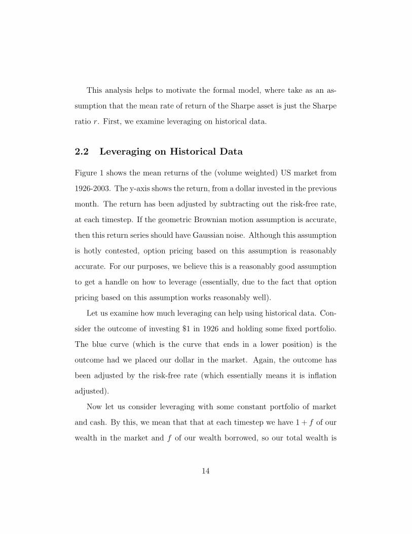
Figure 1: Historical Return. This plot shows the return of the (value weighted)
market from the previous month. The return has been adjusted by the risk free
rate.
We now argue that when the binomial model is a good approximation
to the true geometric Brownian motion, then the mean return of the Sharpe
asset is just the Sharpe ration. The expected return of the Sharpe asset per
dollar is just:
pγ + (1− p)(−1) = pγ + p− 1
and the variance of the Sharpe asset is:
p(1− p)(γ + 1)2
When the binomial model is a good approximation to the market, so p is
close to 0.5 and γ is close to 1. Here, the Sharpe asset has close to unit
variance, and so the mean return of the Sharpe asset is approximately the
Sharpe ratio of the market.
13
This analysis helps to motivate the formal model, where take as an as-
sumption that the mean rate of return of the Sharpe asset is just the Sharpe
ratio r. First, we examine leveraging on historical data.
2.2 Leveraging on Historical Data
Figure 1 shows the mean returns of the (volume weighted) US market from
1926-2003. The y-axis shows the return, from a dollar invested in the previous
month. The return has been adjusted by subtracting out the risk-free rate,
at each timestep. If the geometric Brownian motion assumption is accurate,
then this return series should have Gaussian noise. Although this assumption
is hotly contested, option pricing based on this assumption is reasonably
accurate. For our purposes, we believe this is a reasonably good assumption
to get a handle on how to leverage (essentially, due to the fact that option
pricing based on this assumption works reasonably well).
Let us examine how much leveraging can help using historical data. Con-
sider the outcome of investing $1 in 1926 and holding some fixed portfolio.
The blue curve (which is the curve that ends in a lower position) is the
outcome had we placed our dollar in the market. Again, the outcome has
been adjusted by the risk-free rate (which essentially means it is inflation
adjusted).
Now let us consider leveraging with some constant portfolio of market
and cash. By this, we mean that that at each timestep we have 1 + f of our
wealth in the market and f of our wealth borrowed, so our total wealth is
14

Figure 2: Leveraging the Market. The blue line (ending lower) is the wealth of
the market had we invested 1 dollar in 1926. The series is adjusted for the risk-free
rate of return (which is close to inflation). The red line (ending above the blue
one) uses 200% market and −100% cash (also risk-free rate adjusted). This later
scheme is close to the optimal over this period (the Kelly strategy). The all market
portfolio ends at 160 in 2003, with an average return of 6.8% per year. The Kelly
strategy ends at 800 at an average return of 9.1% per year above the CPI.
1 + f − f = 1. To keep this constant portfolio, we may have to do some
rebalancing — if our wealth rises, we borrow more, while if it falls we pay off
some of our loan.
The red line (ending above the blue) shows the best investment strategy
among those which leverage with some constant fraction. The best constant
leverage turns out to be holding about 200% market and −100% cash. The
return of this portfolio (per timestep) is just:
Kelly return = 2 ∗ (market return− risk-free return)
15
The return of this optimal strategy is termed the Kelly return, because it is
based on the strategy described by Kelly [1956]. The optimal strategy for
maximizing the growth over time is the one which maximizes the log rate of
growth (where the log rate of growth at any given timestep is just log of the
ratio of the wealth at that timestep to the wealth at the previous timestep).
We can also estimate the Sharpe ratio of the market using this historical
data. The Sharpe ratio of the market is r = 0.1214 per month (the time
scale is relevant here, since the ratio of mean to variance depends on the
timescale). We use this parameter in our simulations.
2.3 Wealth Dynamics
We now present the formal model. The time is indexed by t. The wealth at
time t is denoted by Wt. As we have assumed the market evolves according to
a geometric Brownian motion with drift, we make the corresponding assump-
tion that the Sharpe asset also evolves according to a geometric Brownian
motion with drift.
For investment, assume we hold a fraction ft of our wealth in the Sharpe
asset at time t and the remaining 1 − ft in cash. We make the restriction
that ft ∈ [0, 1], so no borrowing is allowed. The model for the evolution of
our wealth is then:
dWt = rftWtdt + ftWtdBt
where dBt is a zero mean, unit variance Brownian motion with unit variance
and r is the Sharpe ratio of the market. We make appropriate measurability
16

assumptions on ft, namely that it is measurable with respect to the history.
Note that the mean drift of the Sharpe asset is just the r, the Sharpe ratio
of the market. In the next subsection, we show that this choice is correct.
In the discrete time version, we have that the change in wealth ∆Wt is
just:
∆Wt = rftWt + ftWtbt
where bt is either 1 or −1, with equal probabilities. We use the discrete
time version in our simulations, since for sufficiently small timesteps, it can
approximate the true continuous time model to arbitrary accuracy.
2.4 The Sharpe Asset, Margins Accounts, & Options
We now discuss the relation of our model to the two standard models. In
the margin account model of the market, one can invest in the market and
borrow cash, subject to the constraint that the investor will not default on
the loan. In the options/cash model, the investor can purchase any option on
the market and hold cash (borrowing is not allowed). In their seminal paper,
Black and Scholes [1973] showed that any investment strategy in margin
account model can be replicated by a portfolio in the option/cash model and
vice versa — under the no arbitrage assumption. By ’replicate’, we mean that
the returns of a strategy in one of these models can be replicated by another
strategy in the other model, with probability 1. Black and Scholes did this
in a continuous time model, with an assumption that the asset behaves as a
geometric Brownian motion. Furthermore, they also showed how to set the
17
price of an option (for any strike price and time period).
In our setting, the investor can only hold the Sharpe asset and cash —
no borrowing is allowed. The following theorem shows this model is entirely
equivalent to the previous two.
Theorem 1 If r in equation 2.3 is set to be the Sharpe ratio of the market,
then any investment strategy in the margin account model of the market —
where the market behaves as a geometric Brownian motion with Sharpe ratio
r — can be replicated in the Sharpe model and vice versa.
proof: (Sketch) Providing a rigorous proof with Ito calculus is beyond
the scope of this paper. A crude sketch is as follows: since the the geometric
Brownian motion model that we have provided can be modeled by the limit
of a binomial model and since we have shown that the Sharpe model and the
Margin account model are equivalent for this binomial model, then in the
limit they are equivalent in the continuous time model.
While these may be formally equivalent, futures may be a more viable
scheme for leveraging for the common investor. Currently, the common in-
vestor often is not able to borrow money close to the risk free rate. Currently,
according to Fidelity, the rate for using a margin account with about 50K$ in
the account is close to 8%, while the risk free rate is currently around 4.5%. 1
Options/futures are priced using a borrowing rate that is essentially the risk-
free rate. This is due to the fact that options/futures are traded just like
1This is outrageous gap, especially since margin accounts are constantly being moni-
tored to prevent a default on the loan.
18

regular equities, so any pricing using higher significantly higher rates (than
the risk-free one) leads to an arbitrage opportunity for some large investment
firm (which is able to borrow at the risk-free rate). Options/futures are a
means by which the common investor can essentially buy on margin at the
risk-free rate. Furthermore, as mentioned in the introduction, funds which
actually leverage for an investor are starting to emerge.
3 The Consumption Model
We first outline the investment decisions and then we specify the utility
functions.
3.1 Dynamics with Income & Spending
At each time t, we make a decision to work or not. If we work at time t, we
assume we obtain one dollar, jt = 1. Of this dollar, we assume that we spend
an amount s and save (i.e. invest) the remaining 1− s dollars. If we do not
work, then our income jt = 0 and we must still spend s out of our savings.
The continuous time version of the model. Here, s is the amount spent per
unit time and jt is the income per unit time t (and again we make appropriate
measurability assumptions on jt). Again letting ft be the amount we invest
in the Sharpe asset, the dynamics of wealth behave as:
dWt = (jt − s + rftWt)dt + ftWtdBt
where again dBt is a zero mean, unit variance Brownian motion. Also, again
19
r is the Sharpe ratio of the Market.
In the discrete time version, we have that the change in wealth ∆Wt is
just:
∆Wt = jt − s + rftWt + ftWtbt (1)
where bt is either 1 or −1, with equal probabilities. Here the work decision jt
is either 1 or 0. And r is the Sharpe ratio defined for this unit of time. Again,
this discrete time version can be made to simulate the continuous version to
arbitrary accuracy.
3.2 Utility for Leisure
Assume we are following some policy π, which decides when to work and
how much to invest in the Sharpe asset at each time. The most natural cost
function to consider is the number of days worked over the infinite horizon.
Due to the Markovian nature of the dynamics and this choice of cost function,
we can restrict ourselves to only consider polices which are functions of the
current wealth.
The cost of the policy π starting from wealth w is then defined to be:
Jπ(w) = E[∫ ∞
0jtdt
∣∣∣∣π, W0 = w]
where we are conditioning on the policy starting at w wealth at time 0. We
are interesting in finding a policy which minimizes Jπ(0).
20

4 Characteristics of the Optimal Life-Cycle
Policy
We define the optimal value function J∗(w) as:
J∗(w) = argminπJπ(w)
We start with a few lemmas on existence, before characterizing the optimal
policy.
4.1 Existence
First, we show that the optimal value function is finite.
Lemma 2 The optimal value function exists and is finite. Furthermore, the
optimal value function is monotonically decreasing. In particular, J∗(w) → 0
as w →∞.
proof: By exhibit a single policy π0 that has finite Jπ0(0) and converges
to zero in the limit of large w we show that these two properties hold for J∗.
The π0 we will consider has the policy of working without doing any investing
up to some fixed target wealth R. At this point the policy will retire and
invest an amount 2s/r in the Sharpe asset. If its wealth ever drops to zero,
it will start working again.
Once retired, the wealth evolves according to a Brownian motion with
positive drift. This probability will then drop off exponentially fast as a
function of R. By choosing R large, we can make the probability of ever
21

returning to zero to be less than .5. Thus Jπ0(0) ≤ 2R < ∞. Further as
wealth goes to infinity, the probability of ever needing to work converges to
zero. Hence, limw→∞ Jπ0(w) = 0.
Clearly if there is a point w′ < w′′ such that J∗(w′) < J∗(w′′) we can
do better at time w′′ by simply burning w′′ − w′ of our wealth. Since this
burning doesn’t increase the strategy space, this is a contradiction.
Unfortunately the above is not sufficient to show that a policy π∗ exists
that obtains J∗. This existence is troubled mostly by issues of measurability.
Lemma 3 There exists a policy π∗ that achieves the lower bound J∗ that is
a measurable function of the wealth.
proof: (sketch) A rigorous proof of this is beyond the scope of this paper.
By a discrete time approximation we can generate a policy that is within
any ε > 0 of J∗. These can all be chosen to be only a function of the
wealth and not the history. Using the discrete time version of the following
theorem, we can restrict ourselves to policies that only have one wealth at
which a switch from working to non-working occurs. Now one can show that
the investment policy has a Lipschitz bound, since if the investment policy
changes too drastically as a function of wealth, then an improved policy exists
which isn’t so drastic. Thus it converges pointwise to a limit.
4.2 Behavior
From this, we have the following natural characterization of the optimal
policy.
22

Theorem 4 There exists some finite wealth, say wretire, such that any op-
timal policy does not work above this wealth (i.e. it works only a measure 0
number of times above this wealth). Conversely, the policy is to works below
this amount.
proof: (sketch) The proof can be summarized by the phrase, “one should
accept all free options.”
By the above lemma we can assume that the optimal policy is only a
function of the wealth. Thus either of the claims would be falsified by finding
two wealths w′ < w′′ such that the policy around the neighborhood of w′ is
to be retired and around the neighborhood of w′′ is to be working. Suppose
we consider the non-Markov policy which instead of working in some small
region around the wealth of w′′ and waits until the wealth drops down to w′
and puts the hours in at that point. At the same time, it runs the current
policy in simulation in order to figure out its investment decisions. Thus
at any point in the future, it will either have the exact same wealth (if the
wealth dropped) or a constant amount less wealth (given the wealth never
dropped). So this is a feasible policy. Further it dominates the claimed
optimal policy. Hence we have a contradiction.
Now let us characterize the retirement policy. It turns out that the re-
tirement policy just minimizes the chance of going bankrupt. We can give a
precise characterization of its behavior.
Theorem 5 The objective of the retirement policy is to minimize the chance
of going ever reaching wretire again. In particular, the probability that re-
23

tirement policy reaches this point from a wealth of w is exp(−
r2(w−wretire)
2s
).
Furthermore, the retirement policy invests a constant amount (not fraction)
in the Sharpe asset, namely 2s/r.
proof:
Define j∗(w) to be 1 if π∗(w) is to work and zero otherwise. Likewise
define f ∗(w) to be the fraction invested by policy π∗(w). Then:
J∗(w) = E(∫ ∞
0j∗(Wt)dt|W0 = w)
= E(j∗(w)h + J∗(Wh)|W0 = w) + o(h)
= j∗(w)h + J∗(w) + J∗′(w)E(Wh|W0 = w)
+J∗′′(w)E(W 2h |W0 = w)/2 + o(h)
where the first equation is by definition, the second is by the smoothing
lemma, and the third is by Taylor’s theorem/Ito calculus. Noting that
E(Wh|W0 = w) = (1 − s + rf ∗(w)w) and E(W 2h |W0 = w) = (f ∗(w)w)2
this reduces to
g(f ∗(w), w) = o(1)
where
g(f, w) = j∗(w) + J∗′(w)(j∗(w)− s + rfw) + J∗′′(w)(fw)2/2.
Thus g(f ∗(w), w) = 0. Further since the amount invested at time t must
be an optimum, we must have that ∂g∂f
(f ∗(w), w) = 0. Solving this shows
f ∗(w)w = −rJ∗′(w)/J∗′′(w).
24

From the equation g(f) = 0
j∗(w) + J∗′(j∗(w)− s− r2J∗′/J∗′′) + (rJ∗′)2/(2J∗′′) = 0.
which is
j∗(w) + J∗′j∗(w)− J∗′s− (rJ∗′)2/(2J∗′′) = 0.
Under retirement (i.e. jt = 0) this simplifies to
2s/r = −rJ∗′/J∗′′
Combining this with our previous equation we get f ∗(w)w = 2s/r during
retirement. So the amount we want to earn is twice what we spend. Solving
the differential equation for J∗′(w) we see that
J∗′(w) = c1er2w/2s
So J∗(w) = c1r2/(2s)er2w/2s + c2. Since we know that J∗(∞) = 0, we know
that c2 = 0.
The previous theorem pretty much tells us what the shape of J∗(w) is for
w ≥ wretire. For small w solving the differential equation is not tractable.
But before we turn to numerical calculations (which most of the rest of the
paper will be about) there are two special cases that are of interest, namely,
s = 1 and s ≈ 0.
4.3 Special Cases
In the special case where s = 1, the differential equation is tractable. In
this case the policy is to invest the amount suggested by “Kelly betting” aka
25
the log-optimal portfolio. Of course, if we start with zero wealth, we never
manage make any profit and stay there forever. Hence J∗(0) = ∞.
The other special case which is solvable is when s ≈ 0. Though we don’t
believe that anyone saves at this rate, it does provide a bound on other rates.
We now sketch out this argument. Suppose that we could choose how much
to work at each point in time (i.e. arbitrary amounts of overtime are allowed.)
The utility is still∫
jtdt but now jt is no longer restricted to be either zero or
one, but is now any non-negative number. In this case, using the arguments
of theorem 4 we see that it is optimal to work as early as possible. Hence
the ratio of our earnings to our spending is arbitrarily high. In other words,
this relaxation moves to the s ≈ 0 domain. Thus the optimal policy is to
work for a small amount of time and then retire. At this point we use the
retirement policy outlined in the previous theorem. If we ever lose all our
money, we again do a small amount of work in an infinitesimal amount of
time. Working out the details of this gives use following theorem:
Theorem 6 Let X be the random variable X =∫
jtdt. For sufficiently small
s, the distribution of X will be arbitrarily close to an exponential distribution
of mean parameter 2s/r2. This holds exactly if jt is allowed to be unbounded.
Note that he arguments that lead to the previous theorem hold if we
define our utility to be E(f(∫
jtdt)) for any monotone function f . This then
allows us to say that certain utility functions do not have any police which
will generate a finite expected utility.
Also note that in this case, J∗(0) = 2s/r2 with the same for the standard
26

deviation. This is then a lower bound for all actual policies we discuss for
which jt is restricted to be either zero or one.
4.4 Extensions
Currently, we have no provision to prevent the policy from switching between
working and not working (perhaps infinitely often or in the continuous time
limit, infinitely quickly). It is straightforward to introduce a switching cost
S for each time the policy switches. The new utility function would then be:
Jπ(w) = E[(#switch)S +
∫jtdt
∣∣∣∣π, W0 = w]
where #switch is the number of switches made between working and not
working.
Here, we can again characterize the optimal policy, which must keep a
memory of when it worked last.
Theorem 7 Assume the switching cost is positive. There exists two finite
wealths, say wretire and wrestart with wretire > wrestart, such that the
optimal policy does not work above the wealth wretire (i.e. it works only a
measure 0 number of times above this wealth), and if the optimal policy ever
drops down to wrestart (after it has passed wretire), then it will start work
again until it obtains wealth greater than wretire.
We do not provide the details of this proof, but it is similar to that of
Theorem 4.
27

Another extension to the model is to allow different spending rate during
work and during retirement. For example, there might be some costs asso-
ciated with employment that aren’t present when retired. In other words,
we have to spend sw when working and sr when retired where sr ≤ sw. To
capture this in our model we rescale by 1/(1+sr−sw). When we are working
we then can save (1−sw)/(1+sr−sw) = 1−sr/(1+sr−sw) whereas when we
are retired we spend sr/(1 + sr − sw). Thus if we figure out a optimal policy
for s = sr/(1 + sr − sw) we also have the optimal policy for this situation.
5 Numerical Results
We now provide simulation based results. Working in the discrete time
model, we computed the optimal policy using dynamic programming based
methods (see Bertsekas [2001]). Essentially, the optimal value function must
satisfy the following Bellman optimality conditions:
J∗(w) = minjt,ft
{jt + E[J∗(w′)|jt, ft]} (2)
where w′ is a random variable, which is the outcome of following the invest-
ment strategy ft, as determined by discrete time dynamics (see equation 1).
We also used the results of the previous section to speed up the compu-
tations. For instance, if the policy was in retirement mode, we used the
analytic formula for the invest policy. Also, we searched over possible retire-
ments wealths, to find the optimal choice.
We used r = 0.1214 as the Sharpe ratio of the market per month, which
28
was estimated from historical data from 1926-2003. In the Sharpe model, the
strategy of 100% market can be replicated by holding 0.056 in the Sharpe
asset and holding the remaining 0.94 in cash. Also, we numerically computed
the Kelly strategy — the one which maximizes the log rate of growth — to
be holding 0.12 in the Sharpe asset and holding the remaining 0.88 in cash.
This turns out to be close to holding about to 200% market and about -100%
cash.
Also, measuring wealth in dollars is rather meaningless, since the scale
of wealth is not specified — we only specify a ratio of spending to saving.
Hence, we state all the wealths in units of yearly income, i.e. wealth is stated
in units of time. For example a wealth of 10 years is equivalent to 10 times
the yearly income.
5.1 Optimal Behavior
Table 4 shows the values starting from 0 wealth for a variety of different
spending ratios and a number of other policies. For instance, the policy
Opt/Opt is the policy which uses the optimal strategy while working and
while retired. Market/Market fully invests in the market both while working
and while retired.
The policy Opt/Market represents using the optimal policy while work-
ing and the market for retirement. Here, we optimized over the choice of the
retirement wealth. Of these (suboptimal) policies, the Kelly/Opt combina-
tion is consistently the best. Essentially, this is because the optimal policy is
29

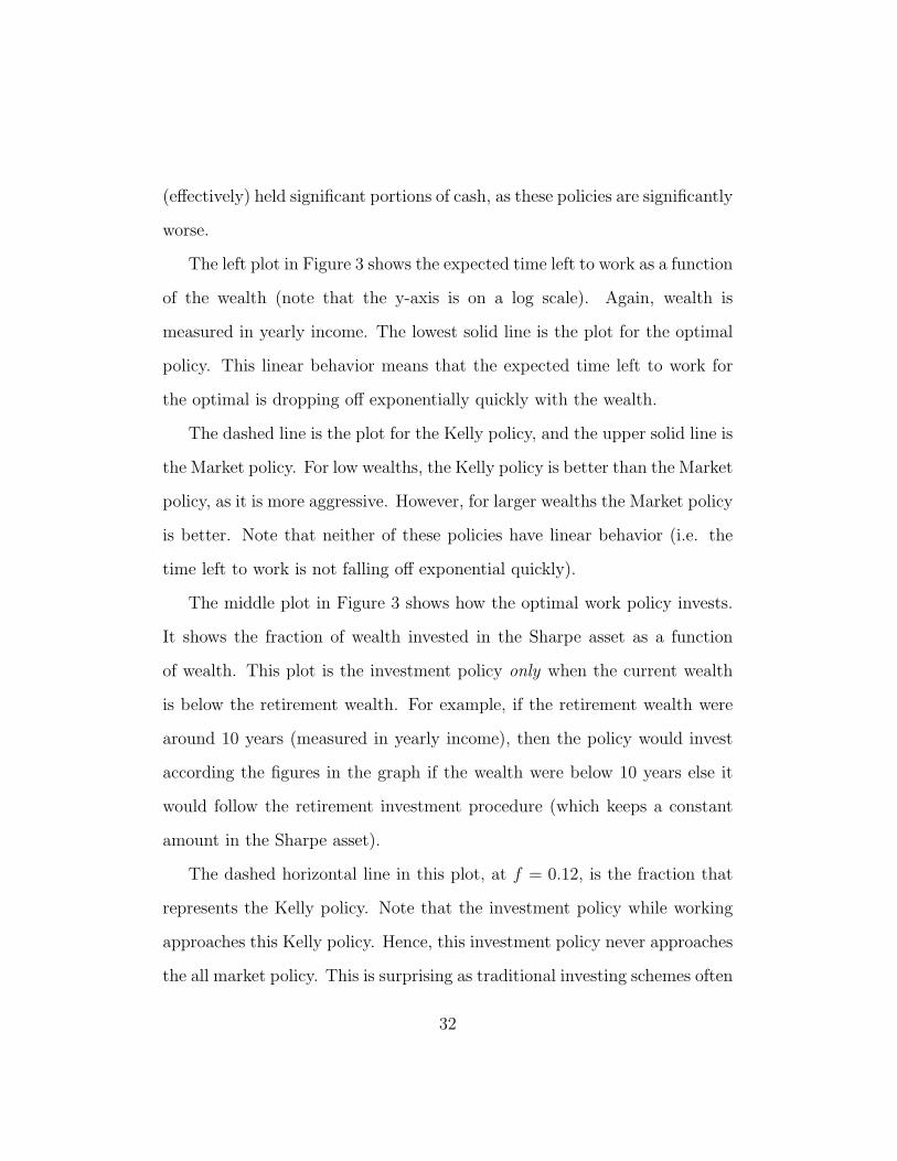
Figure 3: Characteristics of the Optimal Policy. In all plots, wealth is measured
in yearly income. The left plot shows the expected time left to work as a function
of the wealth (note that the y-axis is on a log scale). The lower solid line is Opt,
the dashed line is for Kelly, and the upper solid line is for Market. The middle plot
shows the fraction invested in the Sharpe asset as a function of wealth for the work-
policy. The dashed horizontal line is for Kelly. Note that as Kelly approximately
holds 200% market and −100% cash, the investment strategy while working is
highly leveraged (far more so than traditional investment schemes). The right
plot shows the retirement wealth as a function of the spending ratio, for s = 0.8
with a low and high switching cost. See text for further descriptions.
30

Spending .95 .9 .8 .7 .6 .5
Opt/Opt 32 24 17 13 10 7
Kelly/Opt +4 +5 +4 +3 +2 +3
Opt/Kelly +5 +6 +4 +3 +3 +3
Opt/Market +2 +2 +2 +3 +2 +2
Market/Opt +20 +17 +12 +8 +5 +3
Kelly/Kelly +10 +10 +8 +7 +6 +6
Market/Market +23 +20 +15 +12 +10 +9
lower bound 10 10 9 8 6 5
Figure 4: A Comparison of Strategies. We compare how much better optimal
is than what would traditionally be considered highly risky strategies. The pol-
icy Opt/Market represents the optimal policy while working and investing in the
Market for retirement. The Kelly/Opt is of theoretical interest since it is close to
the Opt/Opt. It is easy to describe: (1) log optimal while working, (2) generate
twice your spending needs from investments while retired. The lower bound is
from Theorem 6 which is tight for small s.
very aggressive while working and Kelly provides reasonable substitute. In
practice, the Kelly/Opt strategy would be the easiest to emulate.
Overall, note how much leveraging helps. For reasonable spending values,
(say around s = 0.8) we can shave off about 15 years of work. This dramatic
improvement is quite robust, even if we use lower values for the Sharpe ratio
(data not shown). We emphasize the s = 0.8 condition as this is the case we
use in most of the other plots. We did not try any unleveraged positions which
31
(effectively) held significant portions of cash, as these policies are significantly
worse.
The left plot in Figure 3 shows the expected time left to work as a function
of the wealth (note that the y-axis is on a log scale). Again, wealth is
measured in yearly income. The lowest solid line is the plot for the optimal
policy. This linear behavior means that the expected time left to work for
the optimal is dropping off exponentially quickly with the wealth.
The dashed line is the plot for the Kelly policy, and the upper solid line is
the Market policy. For low wealths, the Kelly policy is better than the Market
policy, as it is more aggressive. However, for larger wealths the Market policy
is better. Note that neither of these policies have linear behavior (i.e. the
time left to work is not falling off exponential quickly).
The middle plot in Figure 3 shows how the optimal work policy invests.
It shows the fraction of wealth invested in the Sharpe asset as a function
of wealth. This plot is the investment policy only when the current wealth
is below the retirement wealth. For example, if the retirement wealth were
around 10 years (measured in yearly income), then the policy would invest
according the figures in the graph if the wealth were below 10 years else it
would follow the retirement investment procedure (which keeps a constant
amount in the Sharpe asset).
The dashed horizontal line in this plot, at f = 0.12, is the fraction that
represents the Kelly policy. Note that the investment policy while working
approaches this Kelly policy. Hence, this investment policy never approaches
the all market policy. This is surprising as traditional investing schemes often
32

start close to all market and slowly transfer to bonds over time. Our data
suggest that these policies take far longer to reach retirement.
Also, empirically, this work policy is generic — it does not depend on the
choice of the retirement wealth, i.e. it does not depend on the choice of s.
Theoretically, we believe this is true as well, yet we do not have a rigorous
proof of this in the continuous time model. Intuitively, the investment policy
is trying to get over the retirement policy as fast as possible.
5.2 Switching and The Retirement Wealth
We now examine the retirement wealths used by these policies. Note that
while the optimal policy has a fixed retirement wealth, if the policy ever drops
below this wealth it will start working again. In fact, in the continuous time
limit, the optimal policy will switch infinitely often, infinitely quickly.
We impose a switching cost to prevent this behavior. This forces the
optimal policy to wait until the wealth drops down to a certain amount before
it restarts working (see Subsection 4.4). Note that this issue is quite real as
well. For example, after the bubble in the 1990’s, many retired investors had
lost a significant fraction of their wealth — they had to decide whether or
not to restart work.
Table 5 shows the results of using switching costs, with s = 0.8. For
example with low switching cost (penalized by 1 year of work), the optimal
policy switches from retirement to work only 0.5 times on average, brought
down from infinity. The expected number of years worked is 18, slightly
33
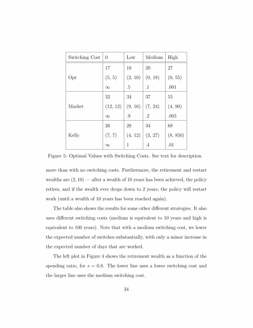
Switching Cost 0 Low Medium High
Opt
17 18 20 27
(5, 5) (2, 10) (0, 18) (0, 55)
∞ .5 .1 .001
Market
32 34 37 55
(12, 12) (9, 16) (7, 24) (4, 90)
∞ .9 .2 .005
Kelly
26 28 34 68
(7, 7) (4, 12) (3, 27) (8, 850)
∞ 1 .4 .01
Figure 5: Optimal Values with Switching Costs. See text for description.
more than with no switching costs. Furthermore, the retirement and restart
wealths are (2, 10) — after a wealth of 10 years has been achieved, the policy
retires, and if the wealth ever drops down to 2 years, the policy will restart
work (until a wealth of 10 years has been reached again).
The table also shows the results for some other different strategies. It also
uses different switching costs (medium is equivalent to 10 years and high is
equivalent to 100 years). Note that with a medium switching cost, we lower
the expected number of switches substantially, with only a minor increase in
the expected number of days that are worked.
The left plot in Figure 4 shows the retirement wealth as a function of the
spending ratio, for s = 0.8. The lower line uses a lower switching cost and
the larger line uses the medium switching cost.
34
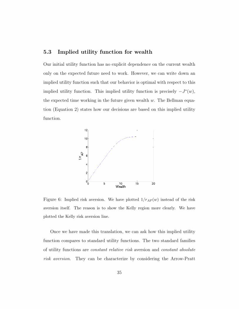
5.3 Implied utility function for wealth
Our initial utility function has no explicit dependence on the current wealth
only on the expected future need to work. However, we can write down an
implied utility function such that our behavior is optimal with respect to this
implied utility function. This implied utility function is precisely −J∗(w),
the expected time working in the future given wealth w. The Bellman equa-
tion (Equation 2) states how our decisions are based on this implied utility
function.
Figure 6: Implied risk aversion. We have plotted 1/rAP (w) instead of the risk
aversion itself. The reason is to show the Kelly region more clearly. We have
plotted the Kelly risk aversion line.
Once we have made this translation, we can ask how this implied utility
function compares to standard utility functions. The two standard families
of utility functions are constant relative risk aversion and constant absolute
risk aversion. They can be characterize by considering the Arrow-Pratt
35

measure of risk aversion, rAP (w) ≡ −U ′′(w)/U ′(w). If this is a constant
function of w then we are said to have constant absolute risk aversion (say,
if U(w) = −e−rw.) If on the other hand, this falls off as 1/w we have a
constant relative risk aversion (say if U(w) = w1+r, or for r = 0 we have
U(w) = log(w)).
We can now describe our utility function as our wealth changes. At first,
we are budget constrained and are highly leveraged. One could think of the
utility as almost being linear. Then after we have some savings, but are still
working, we settle into a constant relative risk aversion utility, so rAP (w)
is growing linearly with 1/w. But we can say more in this regime. rAP (w)
is close to the Kelly (aka log utility) level of risk aversion, namely 1/2w.
Once we retire, we switch to a more conservative utility which has constant
risk aversion. During retirement rAP (w) = 1/2s. The point of retirement is
approximated by when these two cross. These features are shown in Figure 6,
which plots 1/rAP (making both log utility behavior clear (where the plot
behaves linearly) and the conservative behavior clear (where the plot is flat).
Technically, the plot should not have such a smooth bend in it — should
have corner at this place (the smoothing is essentially due to our smoothing
in the computation of the Arrow-Pratt function — which requires numerically
working out discrete derivatives).
36

5.4 The Variance
Table 7 shows the standard deviations of the optimal values in Table 4. The
deviations of these policies are high due to the fact that market is highly
volatile However note that deviations of the Opt/Opt strategy are not par-
ticularly different from the deviation of the all market strategy.
Spending .95 .9 .8 .7 .6 .5
Opt/Opt 22 18 13 11 8 7
Kelly/Opt 20 16 13 10 9 7
Opt/Kelly 26 22 17 13 11 8
Opt/Market 21 18 14 11 9 7
Market/Opt 21 19 16 15 13 10
Kelly/Kelly 25 21 17 14 11 9
Market/Market 19 17 13 11 9 7
Figure 7: Standard Deviations of Strategies. The optimal has fairly low standard
deviation compared to the competitors.
References
[1] Dimitri P. Bertsekas Dynamic Programming and Optimal Control.
Athena Scientific Homepage, 2001.
[2] Black F. and M. Scholes The pricing of options and corporate liabilities.
Journal of Political Economy 81:637, 1973.
37

[3] Brealey, R. A. and Myers, S. C. Principles of Corporate Finance.
McGraw-Hill, 2003.
[4] Cover, T. M. Universal Portfolios. Mathematical Finance, 1991.
[5] E.F. Fama Efficient capital markets: A review of theory and empirical
work. Journal of Finance, 1970
[6] Farhi, E. and Panageas, S. Saving and Investing for Early Retirement:
A Theoretical Analysis. Journal of Financial Economics. Forthcoming.
[7] Kelly, J. A new interpretation of information rate, Bell Systems Technical
Journal, 35, 916-926, , 1956.
[8] Gomes, F. J. and Michaelides, A. Optimal Life-Cycle Asset Allocation:
Understanding the Empirical Evidence. CEPR Discussion Paper No.
4853, 2005.
[9] B. G. Malkiel. A Random Walk Down Wall Street. W. W. Norton and
Company, Inc, New York, 2003
[10] R. C. Merton. Lifetime portfolio selection under uncertainty: The
continuous-time case. Rev. Economics Statist., vol. 51, 1969.
[11] R. C. Merton. Continuous-Time Finance. Blackwell Publishers, 1992.
[12] Sharpe, William F. Mutual Fund Performance. Journal of Business,
1966.
38
[13] Sharpe, William F. Adjusting for Risk in Portfolio Performance Mea-
surement. Journal of Portfolio Management, 1975.
[14] Shreve, S. E. Stochastic Calculus for Finance I: The Binomial Asset
Pricing Model. Springer, 2003.
39


