
DYNAMIC SPATIAL MODELLING:
DIFFERENTIAL EQUATIONS
Derek KarssenbergUtrecht University, the Netherlands
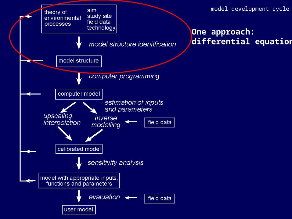
model development cycle.
One approach:differential equations

introductionDifferential equations
• in dynamic models– give rate of change
• mainly point functions
• often used in model structure– vegetation growth– flow of water into or out of storages– radio-active decay– etc, etc
• need to be integrated to be used in a model– analytical– numerical
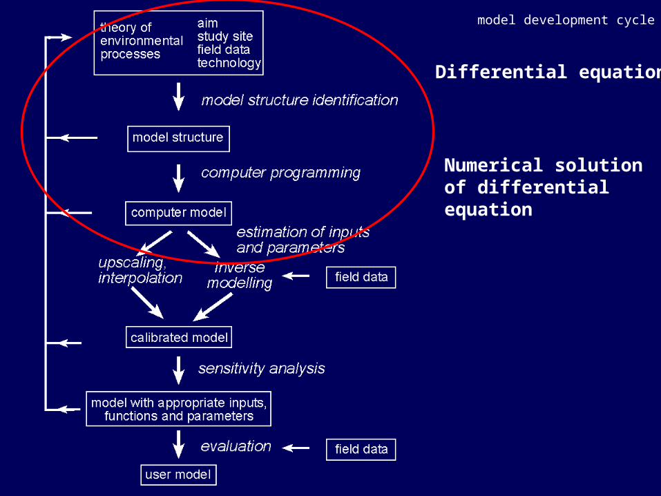
model development cycle.
Differential equation
Numerical solutionof differentialequation

example
What is a differential equation?

exampleExample: interception storage
y amount of water in interception storage (m)k fraction of water in the interception storage that leaves the interception storage per second (s-1, negative value)
time step length (s)

exampleExample: interception storage
k = -0.002 s-1
y(0) = 0.05 m
ttyktytty Δ⋅⋅+=Δ+ )()()(
y(m
)

exampleExample: interception storage
red linek = -0.002 s-1
y(0) = 0.05 m
yellow linek = -0.008 s-1
y(0) = 0.05 m
ttyktytty Δ⋅⋅+=Δ+ )()()(
y(m
)

exampleExample: interception storage
Can be rewritten:
ttyktytty Δ⋅⋅+=Δ+ )()()(

exampleExample: interception storage
By taking the limit :

exampleExample: interception storage
is mostly written as:
This is a differential equation because it involves the derivative
Of the ‘unknown function’
)()(
tykdt
tdy⋅=

exampleExample: interception storage
Note that
Can be written as:
Interpretation: both sides of = give the ‘rate of change’
kydt
dy=
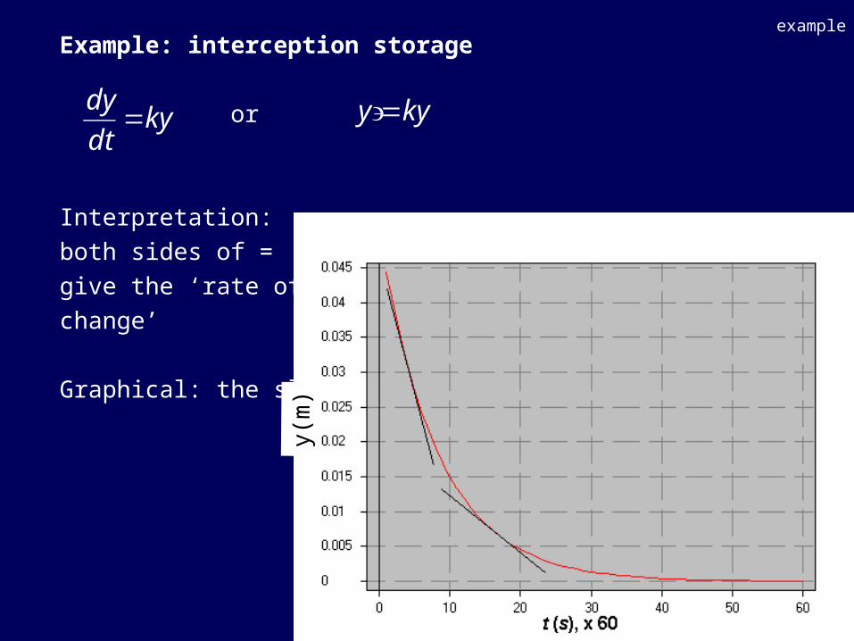
exampleExample: interception storage
or
Interpretation:both sides of =give the ‘rate ofchange’
Graphical: the slope
kydt
dy= kyy ='
y(m
)
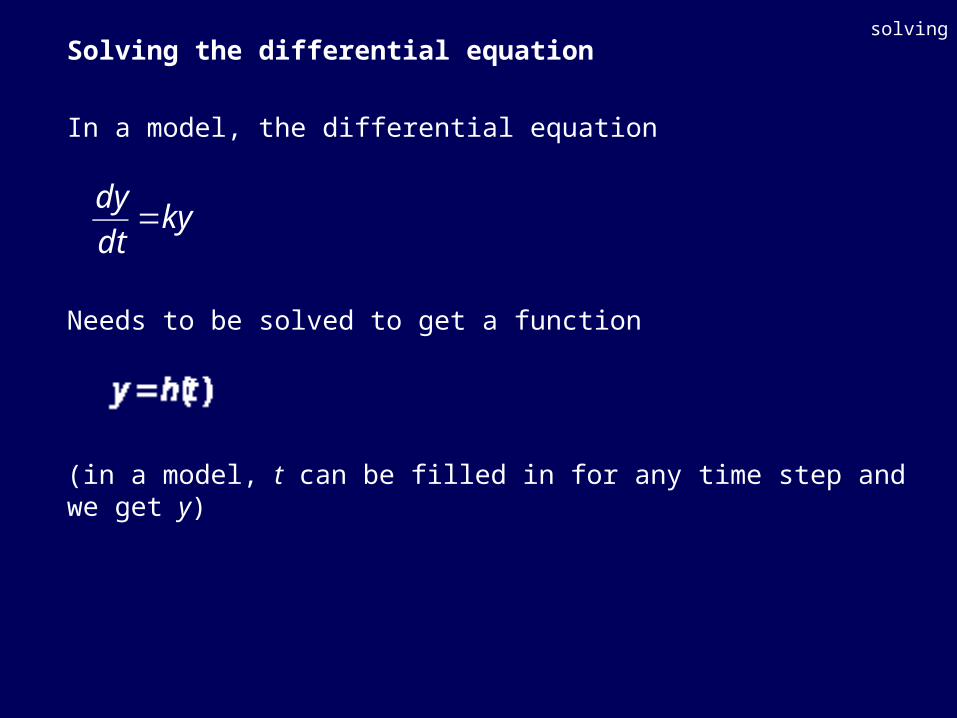
solvingSolving the differential equation
In a model, the differential equation
Needs to be solved to get a function
(in a model, t can be filled in for any time step and we get y)
kydt
dy=

solvingSolving the differential equation
Solving a differential equation can be done in two ways:
• Analytical• Numerical mathematics
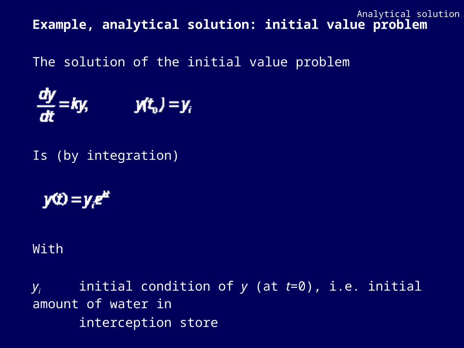
Analytical solutionExample, analytical solution: initial value problem
The solution of the initial value problem
Is (by integration)
With
yi initial condition of y (at t=0), i.e. initial amount of water in
interception store

Analytical solutionAnalytical solution
k=-0.002; # fraction output from canopy (s-1)Dt=60; # timestep (s) timesteps: 60
initial YZero=scalar(0.05); dynamic T=time()*Dt;
Y=YZero*exp(T*k); # Y is not on right side !! report ana.tss=Y;

Analytical solution
y(m
)
Analytical solution
k=-0.002; # fraction output from canopy (s-1)Dt=60; # timestep (s) timesteps: 60
initial YZero=scalar(0.05); dynamic T=time()*Dt;
Y=YZero*exp(T*k); # Y is not on right side !! report ana.tss=Y;

Numerical solutionOften, numerical solutions are used
• Many differential equations cannot be solved analytically
• Numerical solutions are relatively simple to program (not all)
• Numerical solutions are sufficiently precise for most applications
• Modellers can’t do maths...

Numerical solutionMany numerical solution algorithms are available
• Euler method
• Heun’s method
• Runge-Kutta method
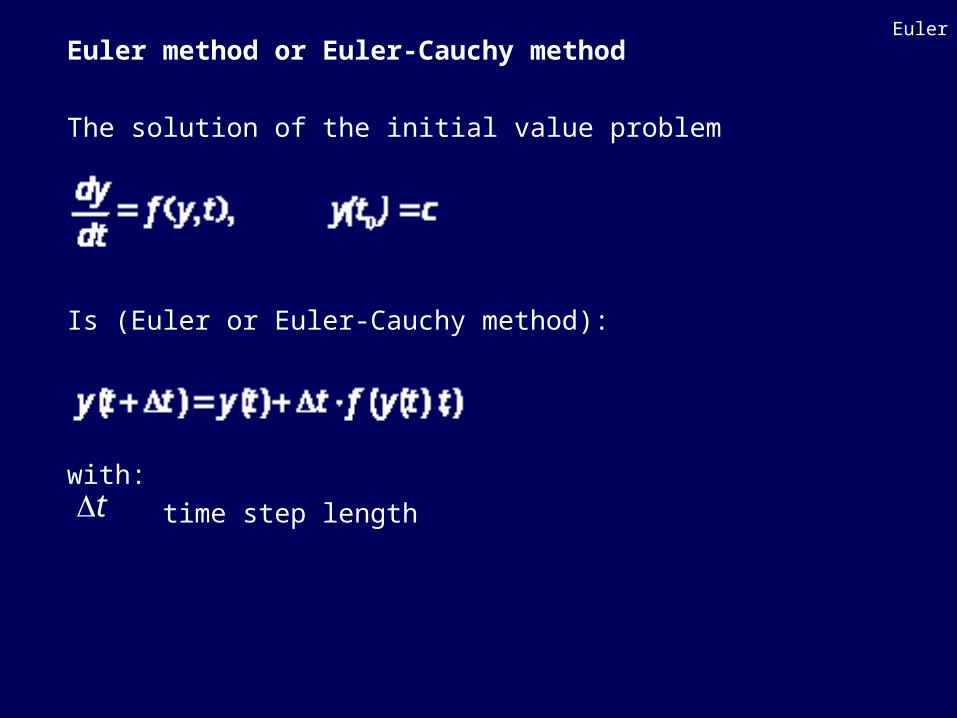
EulerEuler method or Euler-Cauchy method
The solution of the initial value problem
Is (Euler or Euler-Cauchy method):
with:time step lengthtΔ

EulerEuler method or Euler-Cauchy method, example
We have the initial value problem
The solution is: (Euler or Euler-Cauchy method):
Note: this is how we solved it initially

EulerEuler method or Euler-Cauchy method, example
k=-0.002; # fraction output from canopy (s-1)Dt=60; # timestep (s)
timesteps: 60
initial YZero=scalar(0.05); Y=YZero;
dynamic Y=Y+Dt*k*Y; report euler.tss=Y;

Euler.
y(m
)
t(s), x 60

Euler.
t(s), x 60
ab
solu
te e
rror
(m)
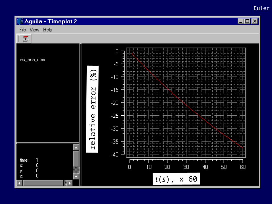
Euler.
t(s), x 60
rela
tive e
rror
(%)

HeunHeun’s method
The solution of the initial value problem
is:
with:
(note: is calculated with Euler’s method)
c)y(ttyfdt
dy== 0 ),,(

HeunHeun’s method, example
We have the initial value problem
The solution is: (Euler or Euler-Cauchy method):
with
iy)y(tkydt
dy== 0 ,

HeunHeun’s method, example
k=-0.002; # fraction output from canopy (s-1)Dt=60; # timestep (s)
timesteps: 60
initial YZero=scalar(0.05); Y=YZero;
dynamic YStar=Y+Dt*k*Y; Y=Y+Dt*((k*Y+k*YStar)/2); report heun.tss=Y;

Heun.
y(m
)
t(s), x 60

Heun.
t(s), x 60
ab
solu
te e
rror
(m)

Heun.
t(s), x 60
ab
solu
te e
rror
(m)
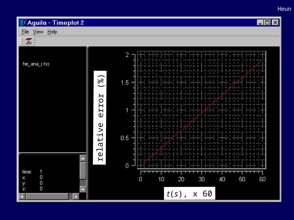
Heun.
t(s), x 60
rela
tive e
rror
(%)

Runge-KuttaClassical Runge-Kutta method of 4th order
- calculate four auxilliarry variables
- derive new value from these
- small numerical error, easy to program

Runge-KuttaClassical Runge-Kutta method of 4th order
We have the initial value problem
The solution is
c)y(ttyfdt
dy== 0 ),,(

Runge-KuttaRunge-Kutta method, example
k=-0.002; # fraction output from canopy (s-1)Dt=60; # timestep (s) timesteps:60
initial YZero=scalar(0.05); Y=YZero;
dynamic KOne=Dt*(k*Y); KTwo=Dt*(k*(Y+0.5*KOne)); KThree=Dt*(k*(Y+0.5*KTwo)); KFour=Dt*(k*(Y+KThree)); Y=Y+(1/6)*(KOne+2*KTwo+2*KThree+KFour); report runga.tss=Y;

Runge-Kutta.
y(m
)
t(s), x 60
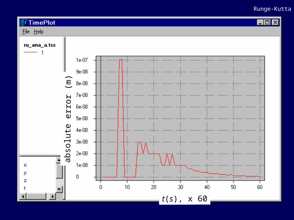
Runge-Kutta.
t(s), x 60
ab
solu
te e
rror
(m)

Runge-Kutta.
t(s), x 60
rela
tive e
rror
(%)

remarksSome conclusions, final remarks
- in many cases, euler method can be used (and is used)- when precision is important, use Runge-Kutta
Not all diff. equations can be solved with Runge-Kutta!- For complicated problems, use pre-programmed software
Example: MODFLOW
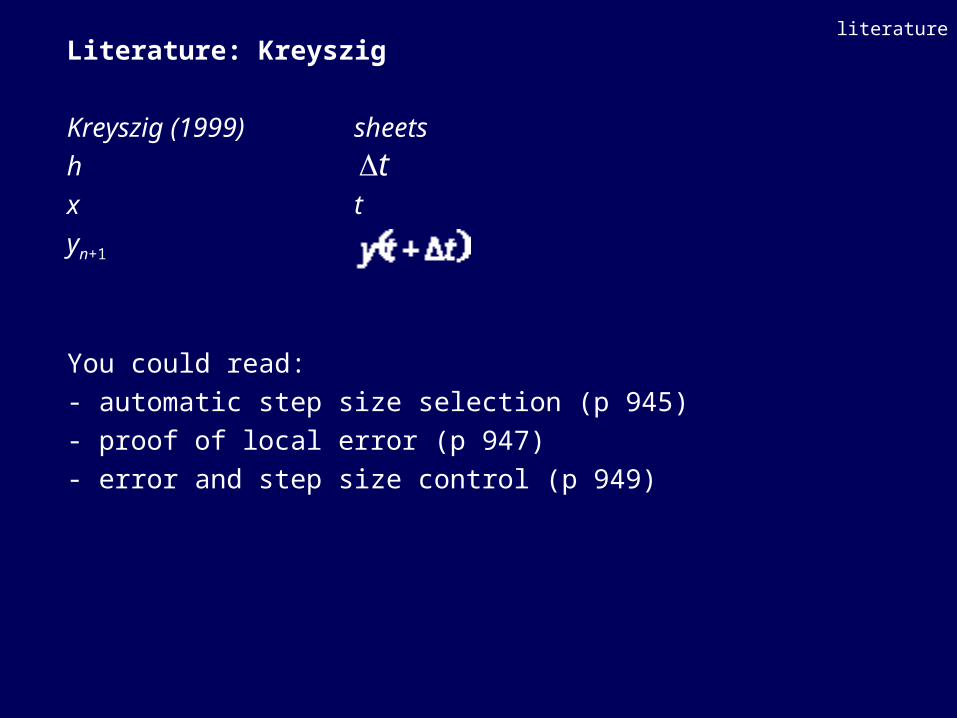
literatureLiterature: Kreyszig
Kreyszig (1999) sheetshx tyn+1
You could read:- automatic step size selection (p 945)- proof of local error (p 947)- error and step size control (p 949)
tΔ


