
Do Ride-sharing Services Affect Traffic Congestion?An Empirical Study of Uber Entry
Ziru LiW. P. Carey School of Business, Arizona State University, [email protected],
Yili HongW. P. Carey School of Business, Arizona State University, [email protected],
Zhongju ZhangW. P. Carey School of Business, Arizona State University, [email protected],
Sharing economy platform, which leverages information technology (IT) to re-distribute unused or under-
utilized assets to people who are willing to pay for the services, has received tremendous attention in the
last few years. Its creative business models have disrupted many traditional industries (e.g., transportation,
hotel) by fundamentally changing the mechanism to match demand with supply in real time. In this research,
we investigate how Uber, a peer-to-peer mobile ride-sharing platform, affects traffic congestion and environ-
ment (carbon emissions) in the urban areas of the United States. Leveraging a unique data set combining
data from Uber and the Urban Mobility Report, we examine whether the entry of Uber car services affects
traffic congestion using a difference-in-difference framework. Our findings provide empirical evidence that
ride-sharing services such as Uber significantly decrease the traffic congestion after entering an urban area.
We perform further analysis including the use of instrumental variables, alternative measures, a relative
time model using more granular data to assess the robustness of the results. A few plausible underlining
mechanisms are discussed to help explain our findings.
Key words : sharing economy, ride-sharing services, digital platforms, traffic congestion
1. Introduction
Platform-based sharing economy, also referred to as collaborative consumption, gig economy or
collaborative economy, has received tremendous attention in recent years. This concept was first
proposed when Benkler (2002) published a paper suggesting that we share goods in economic pro-
1

2
cess. Many studies subsequently explored the potential of the sharing economy (Avital et al. 2014,
Botsman and Rogers 2011, Fellander et al. 2015, Sundararajan 2013, 2014). In 2011, TIME maga-
zine named sharing economy one of the “ten ideas that will change the world”. According to Price
Waterhouse Coopers, five key sharing sectors (P2P finance, online staffing, P2P accommodation,
car sharing and music/video streaming) have the potential to increase global revenues from around
$15 billion to around $335 billion by 2025.1
Although there are many success stories regarding the sharing platforms in recent years, it is
not clear how such platforms could impact the economy and society. In fact, the disruptive force
of the sharing platforms has raised challenges for many incumbent industries as well as policy
makers. Traditional mature industries such as the hotel and the automotive industries were affected
because consumers now have convenient and cost efficient access to resources without the financial,
emotional, or social burdens of ownership (Bardhi and Eckhardt 2015). Sharing economy also
raised debates on regulatory and safety concerns (Feeney and companies Uber 2015, Malhotra and
Van Alstyne 2014). As a result, some traditional companies have tried to lobby the politicians to
regulate the growth of the sharing economy (Wallsten 2015).
As one of the most successful examples of the sharing economy, Uber has raised the most heated
debates. Advocates view Uber services as an important complement to the existing modes of urban
transportation. Others, however, criticize that sharing economy platforms often restructure the
nature of employment and circumvent regulations in order to maximize company benefits. Uber,
for instance, hires drivers as “independent contractors” as opposed to “employees”. Therefore, their
basic rights as workers are not guaranteed. Figure 1 shows a map of the worldwide cities where
Uber operates and where it is banned or is being challenged.
In recent years, researchers have started to examine the effects of the sharing economy (particu-
larly Uber) on social issues. A few studies in this area centered around traffic and transportation
1 http://www.pwc.co.uk/issues/megatrends/collisions/sharingeconomy/the-sharing-economy-sizing-the-
revenue-opportunity.html

3
Figure 1 Where Uber operates, and where it’s been shut down.
Note. Sources: Uber, Bloomberg reporting.
considering Uber is using technology to improve the access and reliability to transportation. For
example, Greenwood and Wattal (2015) found that Uber decreases the rate of alcohol related motor
vehicle homicides. Rayle et al. (2014) used an intercept survey to study the usage and impacts of
ride sharing, and found that it actually fulfills an unserved demand of convenient, point-to-point
urban travel. Wallsten (2015) reveals that Uber’s popularity is associated with the decrease of
consumer complaints about taxi in some cities. A recent report by American Public Transporta-
tion Association2 shows that share modes (car sharing, ride sharing) complement public transit,
decrease car ownership and enhance urban mobility. An important question is does Uber really
have an impact on the traffic congestion in urban areas? There are two countervailing perspectives
(Alexander and Gonzalez 2015) to this question. On one hand, by providing more convenient, less
expensive ride-sharing services, Uber diverts non-driving trips like walking, transit, or cycling to
driving mode. Hence, Uber could induce additional traffic volume and increase traffic congestion.
On the other hand, as a ride-sharing service provider, Uber has the potential to reduce traffic by
diverting trips otherwise made in private, single occupancy cars or taxis.
2 http://www.apta.com/resources/reportsandpublications/Documents/APTA-Shared-Mobility.pdf

4
A few studies have looked into this issue, but the findings are inconclusive. One study from New
York Times estimated that Uber vehicles contribute to about 10 percent of traffic in Manhattan
during evening rush hours, but contended that it’s hard to measure the causal impact of Uber on
the overall traffic increase.3 In a separate study, the Office of the Mayor in New York City released
a report in January 2016, highlighting that the city mayor’s contention that Uber vehicles and
other ride-sharing services had worsened traffic in Manhattan is unfounded.4 In summary, there is
limited empirical evidence to validate arguments on either side.
In this study, we use a natural experiment approach to empirically examine the impact of Uber
on traffic congestion in different urban areas of the United States. This research design offers us
an important advantage: Since the time of Uber entry into various urban areas is different, we
can use a difference-in-difference method to investigate whether the traffic congestion before and
after Uber entry is different across different urban areas. Our data come from multiple sources.
First, the urban mobility report contains different elements of congestion data for each of the
101 urban areas in the United States from 1982 to 2014. Additionally, we conduct comprehensive
due diligence research and collect the entry time of Uber into an urban area from Uber’s official
web site. In order to control the possible effects of other variables, we also collected data on fuel
cost, socio-economic characteristics of the urban areas, characteristics of road transport systems
from United States Census Bureau and Bureau of Economic Analysis. After integrating data from
these sources, we construct an urban area-year level panel data set that includes 957 observations
spanning 11 years over 87 urban areas in the United States.
We find empirical evidence that the entry of Uber actually leads to a significant decrease in traffic
congestion and carbon dioxide emissions in the urban areas of the United States. Moreover, these
results are consistent for different measures of the traffic congestion. To assess the robustness of the
results, we perform further analysis including the use of instrumental variables (IV), alternative
3 http://www.nytimes.com/2015/07/28/upshot/blame-uber-for-congestion-in-manhattan-not-so-fast.html
4 http://www.nytimes.com/2016/01/16/nyregion/uber-not-to-blame-for-rise-in-manhattan-traffic-
congestion-report-says.html

5
measures, and more granular data. We provide a few plausible underlining mechanisms to help
explain our findings. This paper contributes to the existing literature by providing additional
empirical evidence of the social benefits associated with the sharing economy. Additionally, it offers
valuable insights about the broader impact of ride-sharing services on the transportation industry.
The rest of the paper is organized as follows. Section 2 reviews relevant literature on the digital
infrastructure and platforms. Section 3 describe in detail the data and our econometric specifi-
cations. Section 4 presents our findings as well as additional robustness checks. In Section 5, we
discuss our results and provide a few underlining mechanisms to explain the results. Section 6
concludes and provides directions for future research.
2. Literature Review
Digital infrastructure and platforms bring together people, information, and technology to support
business practices, social and economic activities, research, and collective action in civic matters
(Adner and Kapoor 2010, Au and Kauffman 2008, Constantinides and Barrett 2014, Tilson et al.
2010). Research examining the transformative role of digital infrastructure and platforms abound.
Some representative work include Seamans and Zhu (2013), who study the impact of Craigslist
on the classified-ad rates, subscription prices, circulation in the local U.S. newspapers. Chan and
Ghose (2013) investigate whether the entry of Craigslist increases the prevalence of HIV. In a
separate study, Greenwood and Agarwal (2015) also find a significant increase in the HIV incidence
after the introduction of the online matching platform Craigslist. Bapna et al. (2016) estimate the
causal effect of the anonymity feature on matching outcomes on online dating web sites. They find
that anonymous users, who lose the ability to leave a weak signal, end up having fewer matches as
compared to their non-anonymous counterparts.
Crowdfunding is another topic that has received extensive attention in platform research. Wei
and Lin (2015) evaluate two market mechanisms (auctions and posted prices) in online peer-to-
peer lending based on market participants, transaction outcomes, and social welfare. There is also
empirical evidence that home bias exists in online crowdfunding marketplaces for financial products
6
(Lin and Viswanathan 2015). Lin et al. (2013) find that the online friendships of borrowers act as
signals of credit quality in the context of Prosper.com, the largest online P2P lending marketplace.
Burtch et al. (2013) examine both the antecedents and the consequences of the contribution process
in a crowd-funding platform.
Another stream of research on digital platforms examine their impacts on traditional industries
such as the hotel and the transportation industries. Zervas et al. (2016) estimate that each 10%
increase in Airbnb supply results in a 0.37% decrease in monthly hotel room revenue. Wallsten
(2015) explores the competitive effects of ride-sharing on the taxi industry and finds that Uber ’s
popularity decreases the consumer complaints per trip about taxi in New York City and decreases
specific types of complaints about taxi in Chicago.
On-demand, real-time ride-sharing services (e.g., Uber) have similarities with traditional share
modes such as car sharing, but offer some unique characteristics. Alexander and Gonzalez (2015)
explored how ride-sharing affects traffic congestion using mobile phone data and found that under
moderate to high adoption rate scenarios, ride-sharing would likely have noticeable effects in reduc-
ing congested travel times. Fellows and Pitfield (2000) found that car sharing benefits individuals
by halving journey costs and benefits the whole economy by reducing vehicle kilometers, increasing
average speeds and savings in fuel, accidents and emissions. Jacobson and King (2009) investigated
the potential fuel savings in the US when traditional ride-sharing policy was announced and found
that if 10% cars were to have more than one passenger, it could reduce 5.4% annual fuel consump-
tion. Caulfield (2009) estimated the environmental benefits of traditional ride-sharing in Dublin
and found that 12,674t of CO2 emissions were saved by individual ride-sharing.
3. Data and Methods
Our research setting is the Uber platform, the most successful ride-sharing digital platform in the
context of the sharing economy. Officially launched in San Francisco in 2011, Uber has grown from
a small start-up company in Silicon Valley to an international corporation with billions of dollars
of funding. By April 12, 2016, Uber was available in over 60 countries and 404 cities worldwide.

7
Figure 2 Uber’s surge pricing in action
Note. Photo: Uber
Uber ’s two-sided platform business model has made it possible for riders to simply tap their smart-
phones and have a cab arrive at their location in the minimum possible time. When a rider opens
the Uber app, she chooses a ride type (e.g., UberX, UberBlack, UberSUV) and set her location.
The Uber platform automatically assign a driver to the rider request and then the driver on the
other side of the platform respond to the request. The rider will see the driver’s name, picture and
vehicle details, and can track the estimated time of arrival on the map. The pay process is “no
cash, no tip and no hassle”. If the current time period is peak demand time, the customer will face
surge pricing. But they are notified before making the decision, as shown in the Figure2. After a
ride is completed, the rider can rate the driver and provide anonymous feedback about her trip
experience.
3.1. Data
Our data come from a few sources. We retrieved the congestion data from the Urban Mobility
Report (UMR), provided by the Texas A&M Transportation Institute (TTI). The Urban Mobility
Report contains the urban mobility and congestion statistics for each of the 101 urban areas in
the U.S. from 1982 to 2014. This report is acknowledged as the authoritative source of information
about traffic congestion and is widely used in the transportation literature. For each of the urban
areas in the UMR, we searched the official Uber newsroom as well as the major news media to
8
find out if and when Uber arrived in an urban area.5 Fourteen (out of 101) urban areas have Uber
services according to the official Uber web site, but we could not verify the exact Uber entry time
(year and month) into these areas. Hence these areas are not included in our sample. In addition,
given that the earliest Uber entry time (into San Francisco) is 2011, we choose the time window
between 2004 and 2014 to balance the number of time periods before and after the Uber entry. Our
final panel data comprises 957 observations spanning 11 years over 87 urban areas in the United
States.
3.2. Dependent variables
Our target variable is the traffic congestion. We adopted four important indicators from the UMR
to measure congestion. The first measure is the Travel Time Index (TTI), which has been used in
previous studies (Bertini 2006, Hagler and Todorovich 2009, Litman 2007, Mehran and Nakamura
2009, Sweet and Chen 2011, Zhang 2011). TTI refers to the ratio of the travel time in the peak
period to that at free-flow conditions. A value of TTI = 1.20, for example, indicates that a 20-
minute free-flow trip requires 24 minutes during the peak period.
The second variable to measure congestion is the Commuter Stress Index (CSI). CSI refers to the
travel time index calculated for only the peak direction in each peak period. The CSI is believed
to be more indicative of the work trip experienced by each commuter on a daily basis.6 It is worth
noting that both the TTI and the CSI are travel indices and do not represent the actual time of
delay due to congestion.
In order to capture that, we adopted the delay time and the delay cost. Delay time is the amount
of the extra time spent on traveling due to congestion. The delay (congestion) cost refers to the
value of the travel delay, taking into account both the cost of delayed time and the cost of wasted
fuel. Finally, a direct consequence of traffic congestion is the increased level of carbon dioxide
5 There is a slight difference between an urban and a metropolitan area. The urban mobility report is the finest official
data we can get to measure traffic at the urban area.
6 David Schrank, Bill Eisele, Tim Lomax, Jim Bak, “2015 Urban Mobility Scorecard”, Texas Transportation Institute,
http://d2dtl5nnlpfr0r.cloudfront.net/tti.tamu.edu/documents/mobility-scorecard-2015.pdf.

9
emissions from vehicles. In order to analyze the potential environment effect, we use excess fuel
consumption due to congestion to proxy for carbon dioxide emissions. For delay time, delay cost,
and the excess fuel consumption, we adopted both the annual total measurement as well as the
per auto commuter measurements.
Table 1 provides the summary statistics of the eight variables we discussed to measure various
aspects of traffic congestion. Since these variables exhibit significant skewness, we use the log
transformations in our later analysis.
Table 1 Definition and Summary Statistics of Eight Performance Measures of Traffic Congestion
Variable Definition Mean Std. Dev. Min Max
TTI Travel Time Index 1.20 0.08 1.07 1.45
CSI Commuter Stress Index 1.25 0.10 1.07 1.64
DT Annual hours of total
delay (in thousands)
61,401 99,994 2,035 630,722
DTPA Annual hours of delay
per auto commuter
41 12 12 86
DC Annual congestion cost
(million dollars)
1,553 2,492 70 16,346
DCPA Annual congestion cost
per auto commuter($)
1,000 293 323 2,069
EF Annual excess fuel consumed
due to congestion
(Total gallons in thousand)
27,462 41,444 1,106 296,701
EFPA Excess Fuel (gallons
per auto commuter)
18 5 5 35
3.3. Control Variables
We control for the effects of a number of variables including the lane miles of road and the amount
of travelers. These variables have been identified in the previous literature to influence traffic
congestion. Additionally, we control for the variables that may play a role in Uber’s decision to enter

10
different urban areas/cities. These variables include the population size and the socio-economic
status (such as GDP, median income) of an urban area. Table 2 describes the control variables as
well as the summary statistics of these variables.
Table 2 Definition and Summary Statistics of Control Variables
Variable Definition Mean Std. Dev. Min Max
GDP GDP in dollars 119,242 181,231 3,641 1,423,173
POP Population 1,821 2,619 105 19,040
Income Median Income 48,444 8,163 32,875 76,165
FDVMT Freeway Daily Vehicle
Miles of Travel (000)
16,344 21,506 480 139,275
ASDVMT Arterial Street Daily
Vehicle Miles of Travel (000)
16,104 20,184 988 126,010
Commuters Number of auto commuters (000) 825 976 51 5,928
Diesel Cost Average Gasoline Cost ($/gallon) 3.25 0.69 1.77 4.91
Gasoline Cost Average Diesel Cost ($/gallon) 2.92 0.56 1.77 4.35
3.4. Empirical Model and Specification
As discussed earlier, Uber arrives in various urban areas at different points of time. This allows
us to use an exogenous entry model for identification. Specifically, by repeatedly observing the
congestion level in each urban area over time, we could employ a difference-in-difference framework
to examine the difference in congestion before and after Uber entry across multiple areas. Difference-
in-Difference estimation has become an increasingly popular way to estimate causal relationships
(Bertrand et al. 2002). It is appropriate when one wants to compare the difference in outcomes after
and before the intervention for the treated groups to the same difference for the un-treated groups.
In order to control the ex-ante differences between the heterogeneous urban areas, we include area
fixed effects in our model. Our complete model specification is given by:
Congestionit = α+ δ×Uber Entryit +λ×Controlsit + θi + γt + εit (1)

11
where Controlsit represent the control variables for urban area i in year t, α is the grand mean
congestion level. Uber Entryit is a dummy variable. It equals to 1 if urban area i has Uber service
in year t, and zero otherwise. The parameters δ and λ are coefficients; θi and γt represent the urban
area fixed effect and the time fixed effect. Fixed effects capture not only non-time varying factors but
also allow the error term to be arbitrarily correlated with other explanatory variables, thus making
the model estimation robust (Angrist and Pischke 2008). The error term is εit. We use robust
standard errors clustered at the urban areas to deal with potential issues of heteroscedasticity.
4. Results
Tables 3 and 4 present the coefficient estimates of Equation (1) with each column using a different
measure of traffic congestion. It can be seen that the effect of Uber entry is pretty consistent.
The estimate of the effect (except on TTI and Excess fuel per auto) is significant and negative
for all measures of congestion (except for excess fuel per auto). Note that the estimate of Uber
entry on TTI is negative and the p value of the estimate is 0.12, hence marginally significant given
our sample size is only 957 with two way fixed effects. The estimate of Uber entry on Excess fuel
per auto is insignificant (p = 0.615). Overall we find empirical evidence that Uber significantly
decreases traffic congestion in the urban areas of the U.S. It is worth noting that as the median
income in an urban area increases, the traffic tends to get worse. This is consistent with the existing
literature that traffic conditions in a city are usually associated with the overall economic activities.
4.1. Instrumental Variables
In order to address the issue of endogeneity, we identified two instrumental variables (IV) to further
assess the causal relationship between Uber and the traffic congestion. The first instrumental
variable we used is the unemployment rate. From the United States Bureau of Labor Statistics,
we collected data on the unemployment rate of 87 urban areas from 2004 to 2014. This variable
serves as a valid instrument because it is not likely to be correlated with the traffic congestion, but
is an important factor for Uber executives to consider when deciding a go-to market strategy. A
unique feature of Uber’s business model is that it provides flexible job opportunities that attract

12
Table 3 Estimation Results of Uber Entry on Traffic Congestion
(1) (2) (3) (4)TTI CSI DC DCPA
Uber Entry -0.00237+ -0.00377*** -0.0121** -27.32***(0.00151) (0.00139) (0.00600) (7.271)
GDP 0.000364 0.000457 0.00391 3.337(0.000776) (0.000697) (0.00297) (3.424)
Income 0.0515*** 0.0580*** 0.255*** 218.7***(0.0133) (0.0139) (0.0696) (59.51)
Population -0.0230 -0.0274 0.117 9.995(0.0390) (0.0391) (0.141) (188.5)
Commuters -0.0316 -0.0325 0.603*** 739.8***(0.0400) (0.0408) (0.153) (194.6)
Gasoline Cost -0.00335 -0.00919 -0.0505 -48.53(0.0132) (0.0132) (0.0573) (54.28)
Diesel Cost 0.0169 0.0138 0.112 163.9**(0.0154) (0.0157) (0.0889) (78.98)
FDVMT 0.00828 0.00780 0.0748 55.72(0.0138) (0.0148) (0.0659) (69.97)
ASDVMT 0.0185** 0.0130 0.0733* 86.16*(0.00877) (0.00841) (0.0436) (45.61)
Constant 0.745*** 0.815*** -1.985 -7,355***(0.276) (0.286) (1.312) (1,265)
Observations 957 957 957 957Number of urban areas 87 87 87 87R-squared 0.241 0.262 0.478 0.538
1. Cluster-robust standard errors in parentheses. 2. *** p < 0.01, ** p < 0.05, * p < 0.1, +p < 0.15
independent contractors to participate in the labor market. Hence, Uber may be well received in
areas with higher unemployment rates.
Following Angrist and Pischke (2008), we estimate the IV model with the 2SLS approach. Spe-
cially, we estimate the probability that Uber enters an urban area using the standard linear prob-
ability approach and then included it in the second stage estimation. Table 5 reports the results
of this analysis, providing further empirical evidence of our main results. We report the first stage
results and the fit statistics in Table 6. It can be seen that there is a significant correlation between
the IV (unemployment rate) and the Uber entry time (p = 0.018). Additionally, the first stage
F statistics are all significant. Both the CraggDonald Wald F statistics and the Kleibergen-Paap
Wald rk F statistic pass the critical value suggested by Stock and Yogo (2005), alleviating the weak
instrument concern.
We repeated the same analysis using another instrumental variable: percent of population ages
65 and above. The percent of senior citizens is not expected to be correlated with traffic congestion,

13
Table 4 Estimation Results of Uber Entry on Traffic Congestion (cont’d)
(5) (6) (7) (8)DT DTPA EF EFPA
Uber Entry -0.0121** -0.491* -0.0121** 0.210(0.00599) (0.252) (0.00599) (0.133)
GDP 0.00388 0.127 0.00389 0.0652(0.00297) (0.145) (0.00297) (0.0820)
Income 0.256*** 9.674*** 0.256*** 4.746***(0.0692) (2.416) (0.0692) (1.166)
Population 0.118 -5.202 0.118 3.555(0.141) (7.546) (0.141) (4.039)
Commuters 0.599*** -6.314 0.599*** 8.972**(0.153) (7.733) (0.153) (4.112)
Gasoline Cost -0.0499 -1.067 -0.0498 0.316(0.0573) (2.272) (0.0573) (1.148)
Diesel Cost 0.113 5.160* 0.113 1.991(0.0891) (2.621) (0.0891) (1.285)
FDVMT 0.0759 2.361 0.0760 -0.329(0.0660) (2.561) (0.0660) (1.136)
ASDVMT 0.0742* 3.202* 0.0742* 1.181(0.0436) (1.710) (0.0436) (0.821)
Constant 1.534 -42.70 0.784 -124.0***(1.307) (45.01) (1.307) (21.82)
Observations 957 957 957 957Number of urban areas 87 87 87 87R-squared 0.687 0.292 0.687 0.648
1. Cluster-robust standard errors in parentheses. 2. *** p < 0.01, ** p < 0.05, * p < 0.1, +p < 0.15
but may influence the decision by Uber executives to not enter certain urban areas. Previous
research (e.g., Warschauer 2004) have shown that elderly people are more likely to suffer digital
inequalities. Since Uber represents a new phenomenon/trend and is more likely to be adopted by
tech-savvy young generations, it is more (less) likely to offer services in urban areas with a higher
(lower) percentage of young people. Recent statistics of Uber users (both drivers and passengers)
provide anecdotal evidence on our reasoning. From Figure 3, we see that the medium age of Uber
drivers is much younger than that of Taxi drivers. As for passengers, only two percent of Uber
users are over 55 years (Figure 4).
The results of the 2SLS analysis using the percent of population ages 65 and over are presented
in Table 7. The first stage results and the F statistics are reported in Table 8. These results further
strengthen the evidence that Uber significantly reduces traffic congestion in urban areas.

14
Figure 3 Age Range of Uber drivers vs. Taxis drivers
Note. Data source: Hall and Krueger(2015)
Figure 4 Uber’s surge pricing in action
Note. Source: GlobalWebIndex Q2 2015

15
Table 5 2SLS Estimation Results Using Unemployment Rate as the IV
(1) (2) (3) (4) (5) (6) (7) (8)TTI CSI DC DCPA DT DTPA EF EFPA
Uber Entry -0.153** -0.168** -0.745** -821.5** -0.744** -30.88** -0.745** -12.75**(0.0677) (0.0734) (0.327) (346.1) (0.327) (13.37) (0.327) (5.797)
Population 0.364* 0.396* 2.004** 2,055** 73.04* 2.004** 36.93**(0.202) (0.220) (0.978) (1,047) (0.977) (39.98) (0.977) (17.26)
GDP -0.000818 -0.000838 -0.00186 -2.917 -0.00188 -0.113 -0.00188 -0.0369(0.00265) (0.00289) (0.0129) (14.09) (0.0129) (0.528) (0.0129) (0.221)
Income 0.0426 0.0483 0.212 172.0 0.213 7.885 0.213 3.983(0.0315) (0.0347) (0.153) (165.9) (0.153) (6.348) (0.153) (2.730)
Commuters -0.374** -0.408** -1.070 -1,073 -1.072 -75.68** -1.073 -20.62(0.180) (0.196) (0.869) (932.5) (0.868) (35.48) (0.868) (15.38)
Gasoline Cost 0.0267 0.0238 0.0964 110.7 0.0969 5.024 0.0970 2.914(0.0568) (0.0620) (0.279) (300.6) (0.279) (11.50) (0.279) (4.945)
Diesel Cost -0.0209 -0.0276 -0.0723 -35.80 -0.0712 -2.480 -0.0713 -1.268(0.0478) (0.0515) (0.235) (249.6) (0.234) (9.567) (0.234) (4.185)
FDVMT -0.0335 -0.0380 -0.129 -165.3 -0.128 -6.096 -0.128 -3.936(0.0342) (0.0372) (0.164) (175.9) (0.164) (6.782) (0.164) (2.934)
ASDVMT 0.0505* 0.0480 0.229* 255.4* 0.230* 9.676* 0.230* 3.942*(0.0275) (0.0299) (0.134) (143.8) (0.134) (5.512) (0.134) (2.386)
Observations 957 957 957 957 957 957 957 957Number of urban area 87 87 87 87 87 87 87 87R-squared -9.152 -10.210 -6.134 -7.092 -3.281 -11.107 -3.283 -3.545
1. Cluster-robust standard errors in parentheses. 2. *** p < 0.01, ** p < 0.05, * p < 0.1, +p < 0.15
Table 6 IV First Stage Analysis (UnemploymentRate)
Uber Entry Dummy
Unemployment Rate 0.093*(0.050)Population 2.58***(0.74)GDP -0.0077(0.017)Income 0.0076 (0.210)Commuters -2.29***(0.73)Gasoline Cost 0.23 (0.36)Diesel Cost -0.19 (0.30)FDVMT -0.27*(0.18)ASDVMT 0.21 (0.16)Observations 957Number of urban areas 87F statistics 3.37*
1. Cluster-robust standard errors in parentheses. 2.*** p < 0.01, ** p < 0.05, * p < 0.1, +p < 0.15
4.2. Alternative Measure for Uber Entry
So far, we have used Uber entry time to proxy for the implementation of Uber service. This
approach has limitations. Specifically, after Uber service enters an urban area, it takes time for
people to accept and get accustomed to this new service. Therefore, Uber entry may not represent

16
Table 7 2SLS Estimation Results Using Percent of Olds as the IV
(1) (2) (3) (4) (5) (6) (7) (8)TTI CSI DC DCPA DT DTPA EF EFPA
Uber Entry -0.0182* -0.0155+ -0.194** -215.5*** -0.191** -2.106 -0.191** 1.571*(0.00988) (0.00998) (0.0827) (70.69) (0.0819) (1.527) (0.0819) (0.862)
Population 0.0178 0.00274 0.587** 494.6* 0.578** -1.044 0.578** 0.0496(0.0386) (0.0384) (0.265) (262.2) (0.263) (6.104) (0.263) (3.433)
GDP 0.000240 0.000365 0.00247 1.854 0.00248 0.114 0.00248 0.0759(0.000550) (0.000498) (0.00342) (3.612) (0.00336) (0.0889) (0.00336) (0.0675)
Income 0.0505*** 0.0573*** 0.245*** 207.7*** 0.245*** 9.579*** 0.245*** 4.826***(0.00858) (0.00857) (0.0513) (50.56) (0.0506) (1.476) (0.0506) (0.783)
Commuters -0.0678* -0.0593* 0.187 310.2 0.192 -10.00* 0.192 12.08***(0.0348) (0.0345) (0.245) (246.1) (0.242) (5.755) (0.242) (3.234)
Gasoline Cost -0.000179 -0.00685 0.0661 -10.81 -0.0142 -0.743 -0.0140 0.0435(0.0128) (0.0130) (0.0872) (88.46) (0.0863) (2.171) (0.0863) (1.144)
Diesel Cost 0.0129 0.0108 0.0661 116.6 0.0681 4.754** 0.0680 2.333*(0.0128) (0.0128) (0.0821) (77.63) (0.0813) (2.170) (0.0813) (1.202)
FDVMT 0.00387 0.00454 0.0241 3.346 0.0263 1.911 0.0264 0.0501(0.00804) (0.00809) (0.0528) (50.91) (0.0523) (1.416) (0.0523) (0.720)
ASDVMT 0.0219*** 0.0155*** 0.112*** 126.3*** 0.112*** 3.546*** 0.112*** 0.891*(0.00609) (0.00584) (0.0435) (41.65) (0.0430) (1.036) (0.0430) (0.521)
Observations 957 957 957 957 957 957 957 957Number of urban area 87 87 87 87 87 87 87 87R-squared 0.137 0.209 0.069 0.110 0.451 0.260 0.451 0.601
1. Cluster-robust standard errors in parentheses. 2. *** p < 0.01, ** p < 0.05, * p < 0.1, +p < 0.15
Table 8 IV First Stage Analysis (percent of olds)
Uber Entry Dummy
Percent of olds -0.00017**(0.00004)Population 1.994***(0.752)GDP -0.008 (0.018)Income 0.031 (0.198)Commuters -1.921***(0.730)Gasoline Cost 0.065 (0.359)Diesel Cost -0.237 (0.300)FDVMT -0.320*(0.180)ASDVMT 0.198 (0.152)Observations 957Number of urban areas 87F statistics 13.50***
1. Cluster-robust standard errors in parentheses. 2.*** p < 0.01, ** p < 0.05, * p < 0.1, +p < 0.15
the actual usage rate, and there may be a time lag between Uber entry and its impact on the traffic
congestion. In order to alleviate this concern, we use an alternative measure of Uber Entry in urban
areas: the number of Uber searches in an urban area on Google Trends. Google Trends is a publicly
available web application based on Google Search. It provides us an index of the popularity of

17
ride-sharing in a certain geographic region. Google Trends have been previously demonstrated to
track economic activities (retail sales, automotive sales, home sales, and travel) in real time (Choi
and Varian 2012). Wu and Brynjolfsson (2013) find that Google Trends are better in predicting
housing sales and prices than traditional indicators.
We used the Google Trends search history of the keyword combination “Uber” + “name of the
urban area” to measure the popularity and the usage level of Uber in an urban area. It’s reasonable
to assume that when a person search “Uber New York”, she is likely to be interested in the Uber
service in the New York City. Figure 5 plots the search history of Uber service in three cities: San
Francisco, Phoenix, and Austin along with the corresponding actual Uber entry time in each city.
We observe that even though Uber entered San Francisco in June 2011, it only began to become
popular after some time. Similarly, Uber entered Phoenix in October 2012, but began to attract
public attention around 2014. The correlation between Uber entry time and the search volume on
Google is positive and significant.
There is, however, a potential issue with the search volume on Google trends. Before Uber
actually entered an urban area, the search volume is generally not zero in most urban areas. The
non-zero search volume could represent some expectations and curiosity but not the actual Uber
usage. We address this problem by multiplying it with the Uber entry dummy variable as a new
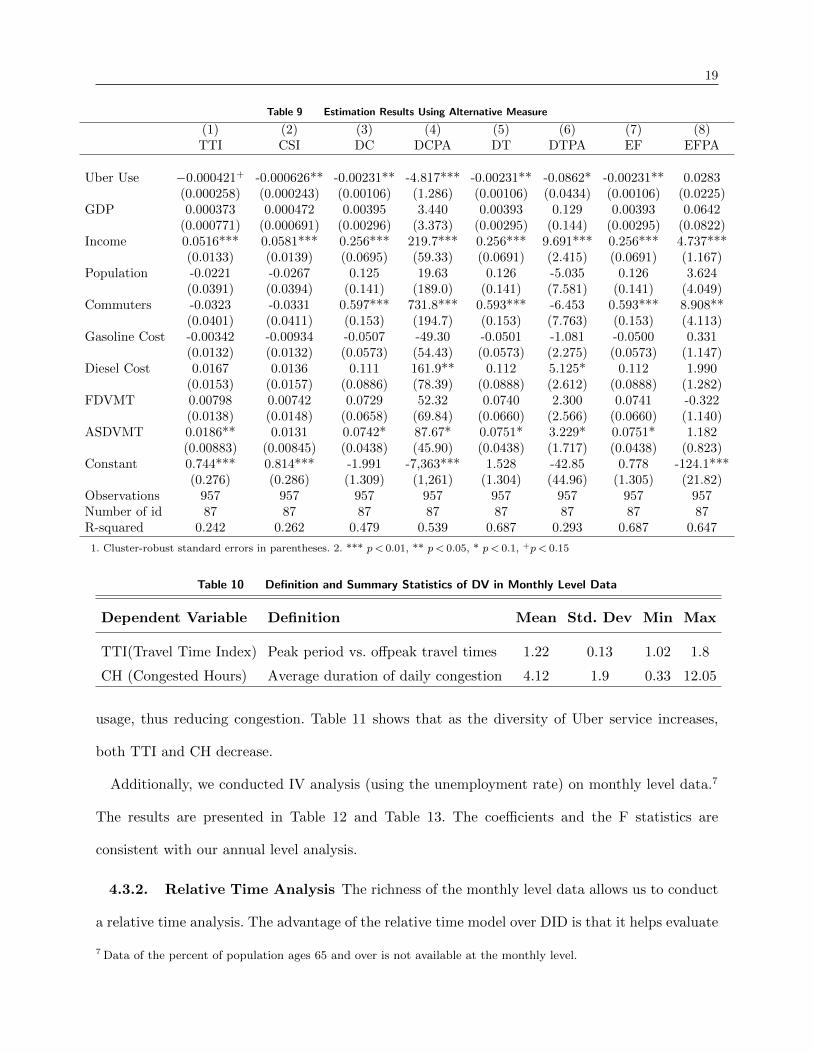
variable: Uber usage. Table 9 presents the results of our analysis using Uber usage. Once again, we
find that our estimation results are robust to this alternative measure.
4.3. Monthly Level Analysis
4.3.1. DID Analysis To further test the robustness of our model, we perform monthly level
analysis. We obtained the monthly traffic data from the Federal Highway Administration (FHWA).
This data set is slightly different from the data set we used for our main analysis. It is monthly level
data ranging from January 2012 to December 2015. The unit of geographic region is Metropolitan
Statistical Area (MSA) instead of urban area. Delay cost, Delay time and excess fuel consumption
are also not available in the monthly level data. As a result, we use TTI and congested hours

18
Figure 5 Time trends of “Uber” + sample urban areas on Google Trends
Note. Source: Google Trends
(CH) as dependent variables in our monthly level data analysis. The summary statistics of the two
variables are shown in Table 10.
We adopt the same DID model and apply it on this new monthly data. Since traffic patterns
exhibit strong seasonal fluctuations, we include the seasonal fixed effect in our model. The results
of the monthly level analysis are shown in Table 11. We can see that the coefficients of Uber entry
are negative and significant for both dependent variables. Another interesting finding is that the
diversity of Uber service has significant and negative effect on congestion. The diversity of Uber
service refers to the number of car types that is available to a customer (Figure 6(a)) when she
opens the app in a geographical area; different car type services come with different fares (Figure
6(b)). We believe that the diversity and multiplicity of Uber services will stimulate more Uber
19
Table 9 Estimation Results Using Alternative Measure
(1) (2) (3) (4) (5) (6) (7) (8)TTI CSI DC DCPA DT DTPA EF EFPA
Uber Use −0.000421+ -0.000626** -0.00231** -4.817*** -0.00231** -0.0862* -0.00231** 0.0283(0.000258) (0.000243) (0.00106) (1.286) (0.00106) (0.0434) (0.00106) (0.0225)
GDP 0.000373 0.000472 0.00395 3.440 0.00393 0.129 0.00393 0.0642(0.000771) (0.000691) (0.00296) (3.373) (0.00295) (0.144) (0.00295) (0.0822)
Income 0.0516*** 0.0581*** 0.256*** 219.7*** 0.256*** 9.691*** 0.256*** 4.737***(0.0133) (0.0139) (0.0695) (59.33) (0.0691) (2.415) (0.0691) (1.167)
Population -0.0221 -0.0267 0.125 19.63 0.126 -5.035 0.126 3.624(0.0391) (0.0394) (0.141) (189.0) (0.141) (7.581) (0.141) (4.049)
Commuters -0.0323 -0.0331 0.597*** 731.8*** 0.593*** -6.453 0.593*** 8.908**(0.0401) (0.0411) (0.153) (194.7) (0.153) (7.763) (0.153) (4.113)
Gasoline Cost -0.00342 -0.00934 -0.0507 -49.30 -0.0501 -1.081 -0.0500 0.331(0.0132) (0.0132) (0.0573) (54.43) (0.0573) (2.275) (0.0573) (1.147)
Diesel Cost 0.0167 0.0136 0.111 161.9** 0.112 5.125* 0.112 1.990(0.0153) (0.0157) (0.0886) (78.39) (0.0888) (2.612) (0.0888) (1.282)
FDVMT 0.00798 0.00742 0.0729 52.32 0.0740 2.300 0.0741 -0.322(0.0138) (0.0148) (0.0658) (69.84) (0.0660) (2.566) (0.0660) (1.140)
ASDVMT 0.0186** 0.0131 0.0742* 87.67* 0.0751* 3.229* 0.0751* 1.182(0.00883) (0.00845) (0.0438) (45.90) (0.0438) (1.717) (0.0438) (0.823)
Constant 0.744*** 0.814*** -1.991 -7,363*** 1.528 -42.85 0.778 -124.1***(0.276) (0.286) (1.309) (1,261) (1.304) (44.96) (1.305) (21.82)
Observations 957 957 957 957 957 957 957 957Number of id 87 87 87 87 87 87 87 87R-squared 0.242 0.262 0.479 0.539 0.687 0.293 0.687 0.647
1. Cluster-robust standard errors in parentheses. 2. *** p < 0.01, ** p < 0.05, * p < 0.1, +p < 0.15
Table 10 Definition and Summary Statistics of DV in Monthly Level Data
Dependent Variable Definition Mean Std. Dev Min Max
TTI(Travel Time Index) Peak period vs. offpeak travel times 1.22 0.13 1.02 1.8
CH (Congested Hours) Average duration of daily congestion 4.12 1.9 0.33 12.05
usage, thus reducing congestion. Table 11 shows that as the diversity of Uber service increases,
both TTI and CH decrease.
Additionally, we conducted IV analysis (using the unemployment rate) on monthly level data.7
The results are presented in Table 12 and Table 13. The coefficients and the F statistics are
consistent with our annual level analysis.
4.3.2. Relative Time Analysis The richness of the monthly level data allows us to conduct
a relative time analysis. The advantage of the relative time model over DID is that it helps evaluate
7 Data of the percent of population ages 65 and over is not available at the monthly level.

20
(a) Uber pickup location screenshot (b) Uber price comparison of different services
Figure 6 Uber offers multiple services with varying price points
Table 11 Estimation Results of Impact of Uber Entry onCongestion using Monthly Level Data
(1) (2)TTI CH
Uber Entry -0.0111* -0.275**(0.00587) (0.121)
Diversity of Uber Service -0.0624*** -1.096***(0.00453) (0.0886)
GDP -0.0592 -112.5(4.381) (58.05)
Personal Income 9.57e-06* 8.68e-05(5.01e-06) (7.24e-05)
Population 0.784 39.85***(0.704) (11.65)
Constant 0.197 -30.12**(0.780) (12.18)
MSA Fixed Effect Yes YesYear Fixed Effect Yes YesSeasonal Fixed Effect Yes YesObservations 2,352 2,352R-squared 0.392 0.294Number of MSA 49 49
1. Cluster-robust standard errors in parentheses. 2. *** p < 0.01,
** p < 0.05, * p < 0.1, +p < 0.15
the parallel trends assumption. According to Angrist and Pischke (2008), the key assumption of
any DID model is the common trend assumption.
Our relative time model is specified in Equation (2). Following David (2003), Bapna et al. (2016),
Chan and Ghose (2013), Greenwood and Wattal (2015), we include a series of time dummies
(j = t−6, ..., t+ 6) that represent the chronological distance between an observation period, t, and
the timing of treatment in MSA i. There are two advantages of this model: 1) it allows us to check
the parallel trend assumption, and 2) it allows us to understand how long it takes for significant

21
Table 12 Estimation Results of IV with Unemployment usingMonthly Level Data
(1) (2)TTI CH
Uber Entry -0.0630*** -0.637+
(0.0240) (0.459)Diversity of Uber Service -0.0630*** -1.100***
(0.00498) (0.0974)GDP 3.485 -87.77**
(2.351) (40.51)Personal Income 3.46e-07 2.25e-05
(5.02e-06) (9.38e-05)Population 0.672 39.06***
(0.601) (11.27)Observations 2,352 2,352R-squared 0.309 0.279Number of MSA 49 49
1. Cluster-robust standard errors in parentheses. 2. *** p < 0.01,
** p < 0.05, * p < 0.1, +p < 0.15
Table 13 IV First Stage Analysis (monthly data)
Uber Entry DummyUnemployment Rate 0.0667 ***(0.327)Unemployment Rate 0.0667 ***(0.327)Control variables IncludedTime and MSA Fixed Effect YesObservations 2352Number of urban areas 49F statistics 33.86***Cragg-Donald Wald F statistic 32.84Kleibergen-Paap Wald rk F statistic 33.86
1. Cluster-robust standard errors in parentheses. 2. *** p < 0.01, **
p < 0.05, * p < 0.1, +p < 0.15
effects to manifest.
Congestionit = α+t+6∑
j=t−6
δj × (µiφ) +λ×Controlsit + θi + γt + εit (2)
In this model, Congestionit represents the two dependent variables: TTI and CH. Since congested
hours is not normally distributed, we log transformed this variable. The variable µi indicates
whether or not Uber will ever enter area i, and φ is the relative time dummies. As before, there
are two kinds of time fixed effects in our model: a year fixed effect and a seasonal fixed effect.
Table 14 presents the results of the relative time analysis. There are several interesting observa-
tions. First these results are consistent with the DID model. In addition, none of the pre-treatment
periods is significant but all the post-treatment periods are significantly negative. This illustrates

22
Table 14 Estimation Results of Relative Time Model usingMonthly Level Data
(1) (2)TTI CH
Rel Timet−6 -0.00543 -0.0518(0.00712) (0.0940)
Rel Timet−5 0.00134 0.0191(0.00819) (0.103)
Rel Timet−4 -0.00437 -0.0852(0.00787) (0.105)
Rel Timet−3 -0.00670 0.0411(0.00627) (0.108)
Rel Timet−2 -0.00847 0.0444(0.00564) (0.106)
Rel Timet−1 OmittedRel Timet -0.0115* -0.137
(0.00614) (0.103)Rel Timet+1 -0.0208*** -0.278**
(0.00597) (0.116)Rel Timet+2 -0.0135** -0.235**
(0.00622) (0.116)Rel Timet+3 -0.0166*** -0.348***
(0.00594) (0.107)Rel Timet+4 -0.0183*** -0.267***
(0.00501) (0.0971)Rel Timet+5 -0.0208*** -0.268***
(0.00468) (0.0938)Rel Timet+6 -0.0145** -0.243***
(0.00700) (0.0885)Diversity of Uber Service -0.0630*** -1.103***
(0.00453) (0.0917)GDP -0.601 -126.5
(4.474) (60.89)Personal Income 1.01e-05* 0.000114
(5.28e-06) (7.39e-05)Population 0.732 39.06***
(0.688) (11.67)Constant 0.257 -29.80**
(0.766) (12.19)MSA Fixed Effect Yes YesYear Fixed Effect Yes YesSeasonal Fixed Effect Yes YesObservations 2,352 2,352R-squared 0.402 0.297Number of MSA 49 49
1. Cluster-robust standard errors in parentheses. 2. *** p < 0.01,** p < 0.05, * p < 0.1, +p < 0.15
that there is no significant difference in common trends. Furthermore a negative and significant
post treatment trend manifests after implementation.

23
5. Discussion
Our extensive analysis provides empirical evidence of a causal relationship between ride-sharing
services and traffic congestion. An important question is what mechanism could possibly drive this
main result. In the following, we offer a few explanations and our insights.
The first possible explanation is that Uber increases vehicle occupancy, thereby decreasing traffic
congestion. Given that the number of commuters in an urban area does not grow at a high rate
over a short period of time, ride sharing can reduce the total number of cars on the road by having
more than one person in the car. A recent survey (Rayle et al. 2014) found that occupancy levels
for ride-sharing vehicles averaged 1.8 passengers in contrast to 1.1 passengers for taxis in a matched
pair analysis. According to the International Energy Agency (2005)8, adding one additional person
to every commute trip could achieve a saving of 7.7% on fuel consumption and a reduction of 12.5%
on vehicle miles.
Second, the low cost travel mode of ride sharing reduces car ownership. In a growing number
of cities, ride-sharing services like Uber provide low cost alternatives to car ownership.9 Take
San Francisco as an example, ride-sharing services are found to reduce car ownership, encourage
more judicious and selective use of cars for particular trip purposes (Cervero and Tsai 2004). The
availability of ride-sharing services also reduces consumers’ incentives to purchase automobiles
(Rogers 2015). Martin and Shaheen (2011) surveyed a sample of 6,281 households and found that
each ride-sharing vehicle replaces 9 to 13 vehicles (postponed and sold) from the road. Another
recent study of North American ride-sharing organizations shows that 15% to 32% of ride-sharing
members sold their personal vehicles, and between 25% and 71% of members avoided an auto
purchase because of ride-sharing.10 A recent survey (Murphy 2016) of more than 4,500 shared
mobility users in the seven study cities (Austin, Boston, Chicago, Los Angeles, San Francisco,
8 http://www.worldenergyoutlook.org/media/weowebsite/2008-1994/weo2005.pdf
9 http://www.usatoday.com/story/money/personalfinance/2014/11/08/ridesharing-lyft-uber/18482083/
10 http://www.rmi.org/Content/Files/North\%20American\%20Carsharing\%20-\%2010\%20Year\
%20Retrospective.pdf

24
Seattle and Washington, DC) also found that people who use more shared modes report lower
household vehicle ownership and decreased spending on transportation.
Third, ride-sharing services can shift demand among different traffic modes. Researchers (Mei-
jkamp 1998, Munheim 1998, Steininger et al. 1996) found evidence that those who used car sharing
services drove significantly less than they did before they had used this service. Katzev (2003)
conducted three studies on the early adopters of Car Sharing Portland and found that this service
promoted trip “bundling” and greater use of alternative transportation such as bus riding, bicy-
cling, and walking. Martin and Shaheen (2011) found that more car sharing users increased their
overall public transit and non-motorized modal use.
Fourth, Uber’s surge pricing strategy has the potential to delay or divert peak hour demands.
The idea behind surge pricing is to adjust prices of rides so as to match driver supply to rider
demand at any given time. Since the price of ride sharing in peak hours can surge quite high, riders
who are price sensitive and flexible in their schedule may delay the travel time or choose to use
public transit instead.
Finally, Uber increases vehicle capacity utilization. According to Cramer and Krueger (2016), in
most cities, the efficiency of Uber is much higher than traditional taxis by having a higher faction of
time and a higher share of miles having fare-paying passengers in their backseats. Higher capacity
utilization means that Uber drivers will spend less time wandering streets searching passengers,
which reduces excess fuel usage and traffic congestion.
6. Conclusion
As sharing economy grows, it is important to examine its potential impacts and implications. This
paper studies one of the many social issues associated with ride-sharing services. Specifically, we
empirically examine how the entry of Uber into major U.S. metropolitan areas influences traffic
congestions. Taking advantage of a natural setting that Uber enters different cities at different
times, we are able to compare the difference in congestion after and before Uber enters an urban area
to the same difference for those urban areas without Uber service. We find that Uber can drastically

25
reduce traffic congestion in urban areas. We performed comprehensive analysis to further assess
the validity of the causal relationship. Our findings are consistent and robust to these extensions.
We searched relevant literature in the transportation industry and summarized a few possible
mechanisms that help explain our results.
This study adds to the ongoing debate over whether and how Uber impacts traffic congestion.
Our rigorous empirical analysis provides additional evidence that on-demand ride sharing could
actually be part of a solution to traffic congestion in major urban areas. This paper also has
practical implications. The expansion of sharing economy faces tremendous challenges over the
last few years. As discussed earlier, many cities have either banned or forced Uber to close down
their business due to various concerns. Our results show that policymakers should also look at the
positive side(s) of the sharing economy in order to make informed decisions.
This study has several limitations. First, we highlight a few mechanisms through which Uber
decreases traffic congestion. Data limitations prevented us from directly testing those hypotheses
in this paper. We call on future studies to further validate the conjectures. Additionally, because
the sharing economy is a relatively new phenomenon, we are unable to examine the longer term
consequences of Uber’s entry on traffic congestion. Future work using longer panel data is worth
to pursue.
References
Adner R, Kapoor R (2010) Value creation in innovation ecosystems: How the structure of technological
interdependence affects firm performance in new technology generations. Strategic management journal
31(3):306–333.
Alexander L, Gonzalez MC (2015) Assessing the impact of real-time ridesharing on urban traffic using mobile
phone data. Proc. UrbComp 1–9.
Angrist JD, Pischke JS (2008) Mostly harmless econometrics: An empiricist’s companion (Princeton univer-
sity press).
Au YA, Kauffman RJ (2008) The economics of mobile payments: Understanding stakeholder issues for an
emerging financial technology application. Electronic Commerce Research and Applications 7(2):141–
164.

26
Avital M, Andersson M, Nickerson J, Sundararajan A, Van Alstyne M, Verhoeven D (2014) The collaborative
economy: a disruptive innovation or much ado about nothing? Proceedings of the 35th International
Conference on Information Systems; ICIS 2014, 1–7 (Association for Information Systems. AIS Elec-
tronic Library (AISeL)).
Bapna R, Ramaprasad J, Shmueli G, Umyarov A (2016) One-way mirrors in online dating: A randomized
field experiment. Management Science .
Bardhi F, Eckhardt GM (2015) The sharing economy isnt about sharing at all. Harvard Business Review
39(4):881–98.
Benkler Y (2002) Coase’s penguin, or, linux and” the nature of the firm”. Yale Law Journal 369–446.
Bertini RL (2006) You are the traffic jam: an examination of congestion measures. Transportation Research
Board, Washington DC .
Bertrand M, Duflo E, Mullainathan S (2002) How much should we trust differences-in-differences estimates?
Technical report, National Bureau of Economic Research.
Botsman R, Rogers R (2011) What’s mine is yours: how collaborative consumption is changing the way we
live (Collins London).
Burtch G, Ghose A, Wattal S (2013) An empirical examination of the antecedents and consequences of
contribution patterns in crowd-funded markets. Information Systems Research 24(3):499–519.
Caulfield B (2009) Estimating the environmental benefits of ride-sharing: A case study of dublin. Trans-
portation Research Part D: Transport and Environment 14(7):527–531.
Cervero R, Tsai Y (2004) City carshare in san francisco, california: second-year travel demand and car
ownership impacts. Transportation Research Record: Journal of the Transportation Research Board
(1887):117–127.
Chan J, Ghose A (2013) Internets dirty secret: assessing the impact of online intermediaries on hiv trans-
mission. MIS Quarterly 38(4):955–976.
Choi H, Varian H (2012) Predicting the present with google trends. Economic Record 88(s1):2–9.
Constantinides P, Barrett M (2014) Information infrastructure development and governance as collective
action. Information Systems Research 26(1):40–56.

27
Cramer J, Krueger AB (2016) Disruptive change in the taxi business: The case of uber. The American
Economic Review 106(5):177–182.
David H (2003) Outsourcing at will: The contribution of unjust dismissal doctrine to the growth of employ-
ment outsourcing. Journal of Labor Economics, January .
Feeney M, companies Uber R (2015) Is ridesharing safe? .
Fellander A, Ingram C, Teigland R (2015) Sharing economy–embracing change with caution. Naringspolitiskt
Forum rapport, number 11.
Fellows N, Pitfield D (2000) An economic and operational evaluation of urban car-sharing. Transportation
Research Part D: Transport and Environment 5(1):1–10.
Greenwood BN, Agarwal R (2015) Matching platforms and hiv incidence: An empirical investigation of race,
gender, and socioeconomic status. Management Science .
Greenwood BN, Wattal S (2015) Show me the way to go home: an empirical investigation of ride sharing
and alcohol related motor vehicle homicide. Fox School of Business Research Paper (15-054).
Hagler Y, Todorovich P (2009) Where high-speed rail works best (America 2050).
Jacobson SH, King DM (2009) Fuel saving and ridesharing in the us: Motivations, limitations, and oppor-
tunities. Transportation Research Part D: Transport and Environment 14(1):14–21.
Katzev R (2003) Car sharing: A new approach to urban transportation problems. Analyses of Social Issues
and Public Policy 3(1):65–86.
Lin M, Prabhala NR, Viswanathan S (2013) Judging borrowers by the company they keep: Friendship
networks and information asymmetry in online peer-to-peer lending. Management Science 59(1):17–35.
Lin M, Viswanathan S (2015) Home bias in online investments: An empirical study of an online crowdfunding
market. Management Science 62(5):1393–1414.
Litman T (2007) Evaluating rail transit benefits: A comment. Transport Policy 14(1):94–97.
Malhotra A, Van Alstyne M (2014) The dark side of the sharing economy and how to lighten it. Communi-
cations of the ACM 57(11):24–27.

28
Martin EW, Shaheen SA (2011) Greenhouse gas emission impacts of carsharing in north america. IEEE
Transactions on Intelligent Transportation Systems 12(4):1074–1086.
Mehran B, Nakamura H (2009) Considering travel time reliability and safety for evaluation of congestion
relief schemes on expressway segments. IATSS research 33(1):55–70.
Meijkamp R (1998) Changing consumer behaviour through eco-efficient services: an empirical study of car
sharing in the netherlands. Business Strategy and the Environment 7(4):234–244.
Munheim P (1998) Car sharing studies: An investigation. Lucerne, Switzerland .
Murphy C (2016) Shared mobility and the transformation of public transit. Technical report.
Rayle L, Shaheen S, Chan N, Dai D, Cervero R (2014) App-based, on-demand ride services: Comparing taxi
and ridesourcing trips and user characteristics in san francisco university of california transportation
center (uctc). Technical report, UCTC-FR-2014-08.
Rogers B (2015) The social costs of uber. University of Chicago Law Review Dialogue, Forthcoming .
Seamans R, Zhu F (2013) Responses to entry in multi-sided markets: The impact of craigslist on local
newspapers. Management Science 60(2):476–493.
Steininger K, Vogl C, Zettl R (1996) Car-sharing organizations: The size of the market segment and revealed
change in mobility behavior. Transport Policy 3(4):177–185.
Stock JH, Yogo M (2005) Testing for weak instruments in linear iv regression. Identification and inference
for econometric models: Essays in honor of Thomas Rothenberg .
Sundararajan A (2013) From zipcar to the sharing economy. Harvard Business Review 1.
Sundararajan A (2014) Peer-to-peer businesses and the sharing (collaborative) economy: Overview, economic
effects and regulatory issues. Written testimony for the hearing titled The Power of Connection: Peer
to Peer Businesses, January .
Sweet MN, Chen M (2011) Does regional travel time unreliability influence mode choice? Transportation
38(4):625–642.
Tilson D, Lyytinen K, Sørensen C (2010) Research commentary-digital infrastructures: the missing is research
agenda. Information systems research 21(4):748–759.

29
Wallsten S (2015) The competitive effects of the sharing economy: how is uber changing taxis? Technology
Policy Institute .
Wei Z, Lin M (2015) Market mechanisms in online crowdfunding. Available at SSRN 2328468 .
Wu L, Brynjolfsson E (2013) The future of prediction: How google searches foreshadow housing prices and
sales. Available at SSRN 2022293 .
Zervas G, Proserpio D, Byers J (2016) The rise of the sharing economy: Estimating the impact of airbnb on
the hotel industry. Boston U. School of Management Research Paper (2013-16).
Zhang Y (2011) Hourly traffic forecasts using interacting multiple model (imm) predictor. IEEE Signal
Processing Letters 18(10):607–610.


