Distributed Model:
Petri Nets

Introduc4on
• Introduced by Carl Adam Petri in 1962.
• A diagramma4c tool to model concurrency and synchroniza4on in distributed systems.
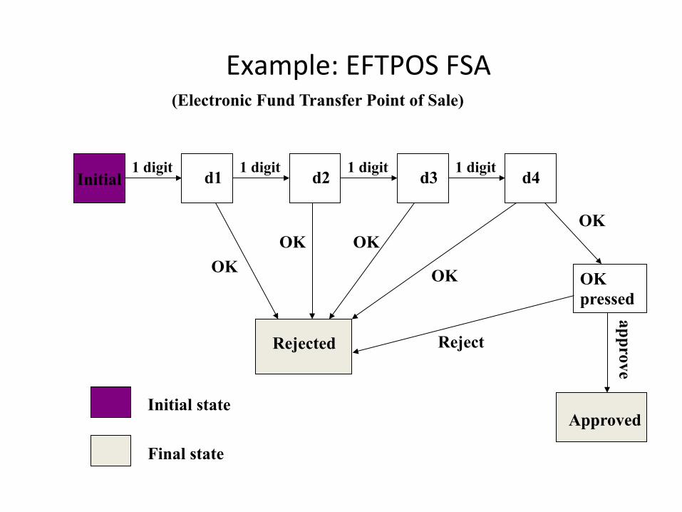
Example: EFTPOS FSA
Initial 1 digit 1 digit 1 digit 1 digit d1 d2 d3 d4
OK
OK pressed
approve
Approved
Rejected
OK
OK OK OK
Initial state
Final state
Reject
(Electronic Fund Transfer Point of Sale)
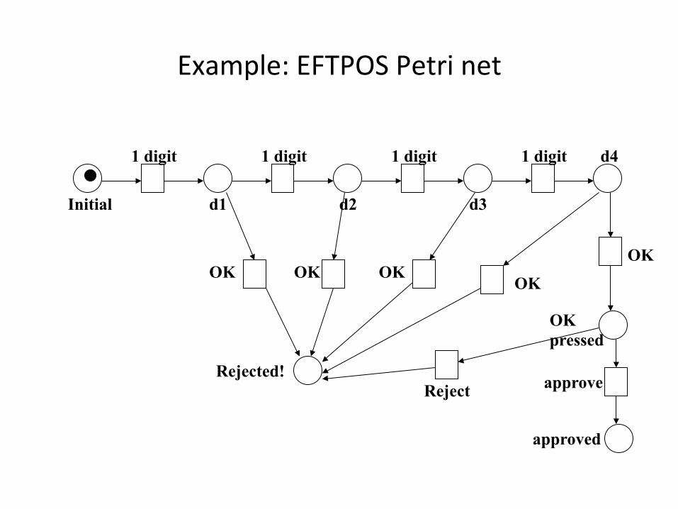
Example: EFTPOS Petri net
Initial
1 digit 1 digit 1 digit 1 digit
d1 d2 d3
d4
OK
OK pressed
approve
approved
OK OK OK OK
Reject Rejected!
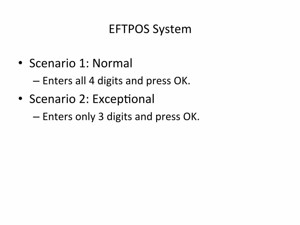
EFTPOS System
• Scenario 1: Normal – Enters all 4 digits and press OK.
• Scenario 2: Excep4onal – Enters only 3 digits and press OK.
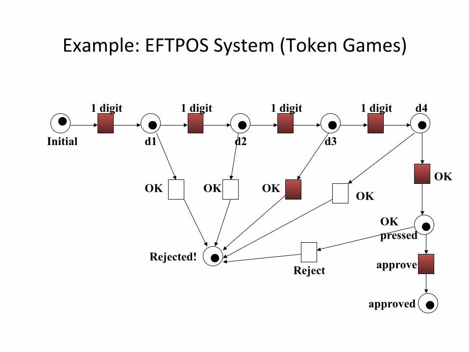
Example: EFTPOS System (Token Games)
Initial
1 digit 1 digit 1 digit 1 digit
d1 d2 d3
d4
OK
OK pressed
approve
approved
OK OK OK OK
Reject Rejected!

A Petri Net Specifica4on ...
• consists of: places (circles), transi+ons (rectangles) and arcs (arrows): – Places represent possible states of the system. – Transi+ons are events or ac4ons which cause the change of state.
– Every arc simply connects a place with a transi4on or a transi4on with a place.
A Change of State …
• is denoted by a movement of token(s) (black dots) from place(s) to place(s); and is caused by the firing of a transi4on.
• The firing represents an occurrence of the event or an ac4on taken.
• The firing is subject to the input condi4ons, denoted by token availability.

A Change of State
• A transi4on is firable or enabled when there are sufficient tokens in its input places.
• AYer firing, tokens will be transferred from the input places (old state) to the output places, deno4ng the new state.
• Note that the EFTPOS example is a Petri net representa4on of a finite state machine (FSM).
Example: Vending Machine
• The machine dispenses two kinds of snack bars – 20c and 15c.
• Only two types of coins can be used – 10c coins and 5c coins.
• The machine does not return any change.

Example: Vending Machine (STD of an FSM)
0 cent
5 cents
10 cents
15 cents
20 cents
Deposit 10c
Deposit 10c D
eposit 5c
Deposit 5c
Take 20c snack bar
Take 15c snack bar
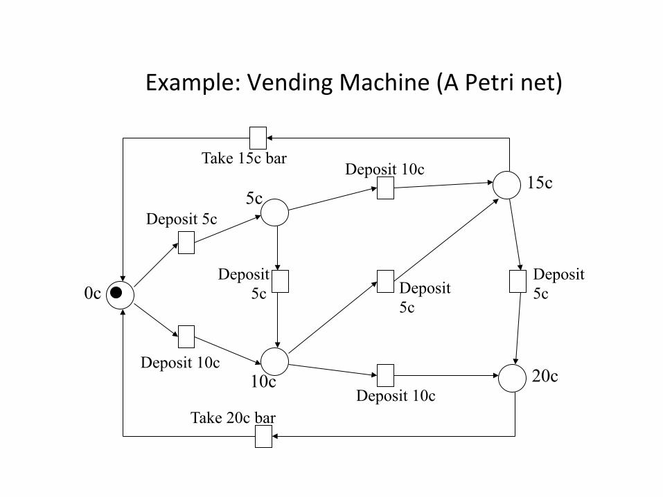
Example: Vending Machine (A Petri net)
5c
Take 15c bar
Deposit 5c
0c
Deposit 10c
Deposit 5c
10c
Deposit 10c
Deposit 5c
Deposit 10c 20c
Deposit 5c
15c
Take 20c bar

Example: Vending Machine (3 Scenarios)
• Scenario 1: – Deposit 5c, deposit 5c, deposit 5c, deposit 5c, take 20c snack bar.
• Scenario 2: – Deposit 10c, deposit 5c, take 15c snack bar.
• Scenario 3: – Deposit 5c, deposit 10c, deposit 5c, take 20c snack bar.

Example: Vending Machine (Token Games)
5c
Take 15c bar
Deposit 5c
0c
Deposit 10c
Deposit 5c
10c
Deposit 10c
Deposit 5c
Deposit 10c 20c
Deposit 5c
15c
Take 20c bar

Mul4ple Local States
• In the real world, events happen at the same 4me.
• A system may have many local states to form a global state.
• There is a need to model concurrency and synchroniza4on.

Example: In a Restaurant (A Petri Net)
Waiter free Customer 1 Customer 2
Take order
Take order
Order taken
Tell kitchen
wait wait
Serve food Serve food
eating eating
Example: In a Restaurant (Two Scenarios)
• Scenario 1: – Waiter takes order from customer 1; serves customer 1; takes order from customer 2; serves customer 2.
• Scenario 2: – Waiter takes order from customer 1; takes order from customer 2; serves customer 2; serves customer 1.
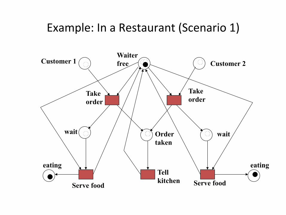
Example: In a Restaurant (Scenario 1)
Waiter free Customer 1 Customer 2
Take order
Take order
Order taken
Tell kitchen
wait wait
Serve food Serve food
eating eating

Example: In a Restaurant (Scenario 2)
Waiter free Customer 1 Customer 2
Take order
Take order
Order taken
Tell kitchen
wait wait
Serve food Serve food
eating eating

Transi4on (firing) rule • A transi4on t is enabled if each input place p has at least w(p,t) tokens
• An enabled transi4on may or may not fire • A firing on an enabled transi4on t removes w(p,t) from each input place p, and adds w(t,p') to each output place p'
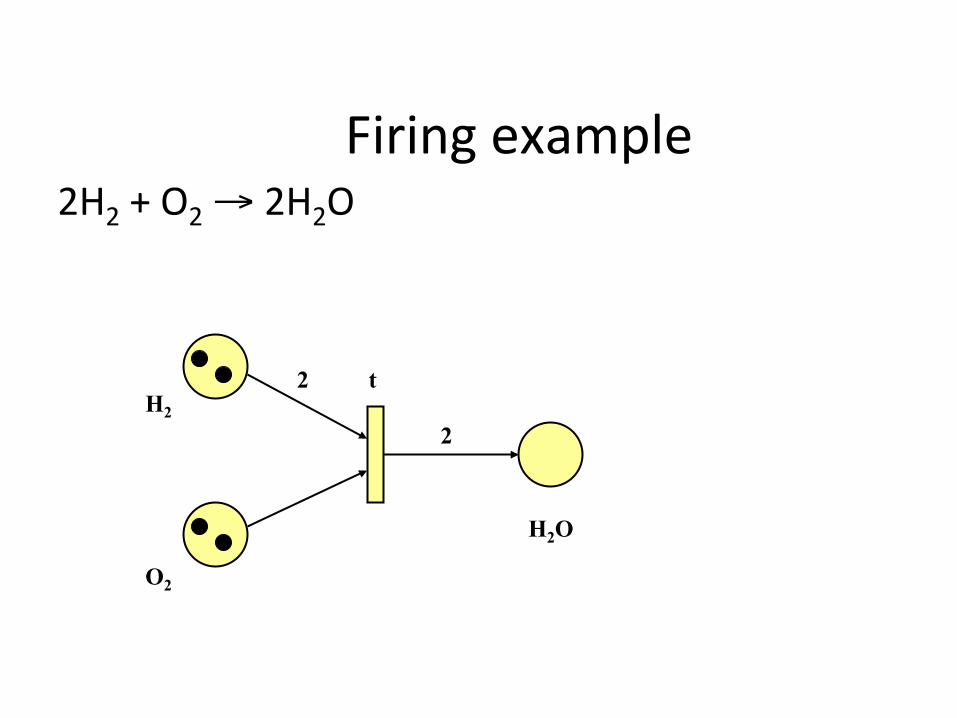
Firing example 2H2 + O2 → 2H2O
H2
O2
H2O
t
2
2

Firing example 2H2 + O2 → 2H2O
H2
O2
H2O
t
2
2

Some defini4ons • source transi,on: no inputs • sink transi,on: no outputs • self-‐loop: a pair (p,t) s.t. p is both an input and an output of t • pure PN: no self-‐loops • ordinary PN: all arc weights are 1's • infinite capacity net: places can accommodate an unlimited number of
tokens • finite capacity net: each place p has a maximum capacity K(p) • strict transi,on rule: aYer firing, each output place can't have more than
K(p) tokens • Theorem: every pure finite-‐capacity net can be transformed into an
equivalent infinite-‐capacity net

Modeling FSMs
15
20 10
5
10
vend 15¢ candy
10
5 5
10
5
vend 20¢ candy
0
5

Modeling FSMs
5 10
vend 15¢ candy
10
5
5
10
5
vend 20¢ candy
state machines: each transition has exactly one input and one output

Modeling FSMs
5 10
vend
10
5
5
10
5
vend
conflict, decision or choice

Net Structures
• A sequence of events/ac4ons:
• Concurrent execu4ons:
e1 e2 e3
e1
e2 e3
e4 e5

Net Structures
• Non-‐determinis4c events -‐ conflict, choice or decision: A choice of either e1, e2 … or e3, e4 ...
e1 e2
e3 e4

Net Structures
• Synchroniza4on
e1

Net Structures
• Synchroniza4on and Concurrency
e1
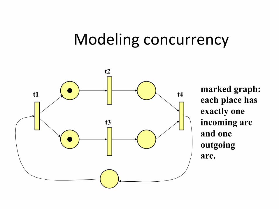
Modeling concurrency
t2
t3
t1 t4 marked graph: each place has exactly one incoming arc and one outgoing arc.

Modeling concurrency
t2
t3
t1 t4
concurrency

Modeling dataflow computa4on
x = (a+b)/(a-‐b)
a
a
b
b
a+b
a-b
+
-
/
≠0
=0
x
NaN
copy
copy

Modeling communica4on protocols
ready to send
wait for ack.
ack. received
msg. received
ack. sent
ready to receive
buffer full
buffer full send
msg.
receive ack.
receive msg.
send ack.
proc.1
proc.2

Modeling synchroniza4on control
writing k reading
k
k
k

Another Example
• A producer-‐consumer system, consist of one producer, two consumers and one storage buffer with the following condi4ons: • The storage buffer may contain at most 5 items. • The producer sends 3 items in each produc4on. • At most one consumer is able to access the storage buffer at one 4me.
• Each consumer removes two items when accessing the storage buffer.

A Producer-‐Consumer System
ready p1
t1 produce
idle
send
p2
t2
k=1
k=1
k=5
Storage p3
3 2 t3 t4
p4
p5
k=2
k=2
accept
accepted
consume
ready
Producer Consumers
A Producer-‐Consumer Example
• In this Petri net, every place has a capacity and every arc has a weight.
• This allows mul4ple tokens to reside in a place to model more complex behaviour.

Behavioural Proper4es
• Reachability • “Can we reach one par4cular state from another?”
• Boundedness • “Will a storage place overflow?”
• Liveness • “Will the system die in a par4cular state?”
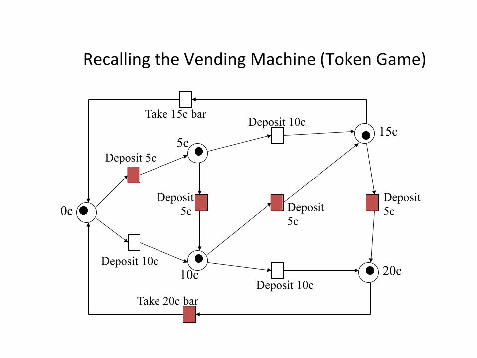
Recalling the Vending Machine (Token Game)
5c
Take 15c bar
Deposit 5c
0c
Deposit 10c
Deposit 5c
10c
Deposit 10c
Deposit 5c
Deposit 10c 20c
Deposit 5c
15c
Take 20c bar

A marking is a state ...
t8
t1
p1
t2
p2
t3
p3
t4
t5
t6 p5
t7
p4
t9
M0 = (1,0,0,0,0) M1 = (0,1,0,0,0) M2 = (0,0,1,0,0) M3 = (0,0,0,1,0) M4 = (0,0,0,0,1)
Initial marking:M0

Reachability t8
t1
p1
t2
p2
t3
p3
t4
t5
t6 p5
t7
p4
t9
Initial marking:M0
M0 M1 M2 M3 M0 M2 M4 t3 t1 t5 t8 t2 t6
M0 = (1,0,0,0,0)
M1 = (0,1,0,0,0)
M2 = (0,0,1,0,0)
M3 = (0,0,0,1,0)
M4 = (0,0,0,0,1)

Reachability
• “M2 is reachable from M1 and M4 is reachable from M0.”
• In fact, in the vending machine example, all markings are reachable from every marking.
M0 M1 M2 M3 M0 M2 M4 t3 t1 t5 t8 t2 t6
A firing or occurrence sequence:

Boundedness
• A Petri net is said to be k-‐bounded or simply bounded if the number of tokens in each place does not exceed a finite number k for any marking reachable from M0.
• The Petri net for vending machine is 1-‐bounded.
• A 1-‐bounded Petri net is also safe.
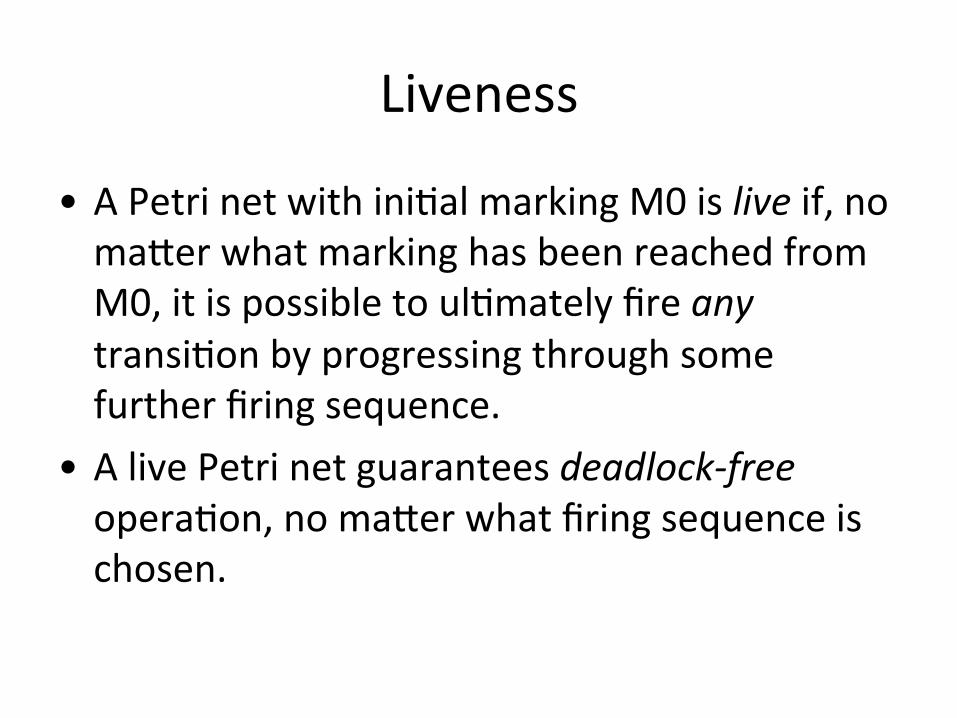
Liveness
• A Petri net with ini4al marking M0 is live if, no maler what marking has been reached from M0, it is possible to ul4mately fire any transi4on by progressing through some further firing sequence.
• A live Petri net guarantees deadlock-‐free opera4on, no maler what firing sequence is chosen.

Liveness
• The vending machine is live and the producer-‐consumer system is also live.
• A transi4on is dead if it can never be fired in any firing sequence.

An Example
A bounded but non-live Petri net
p1 p2
p3
p4
t1
t2
t3 t4
M0 = (1,0,0,1)
M1 = (0,1,0,1)
M2 = (0,0,1,0)
M3 = (0,0,0,1)
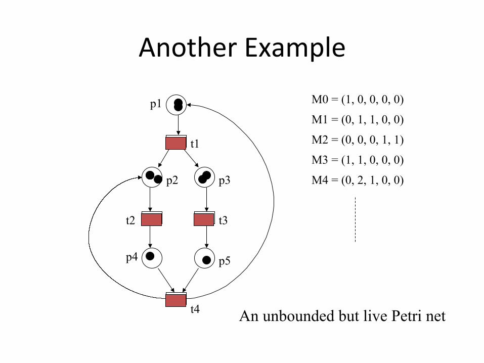
Another Example
p1
t1
p2 p3
t2 t3
p4 p5
t4 An unbounded but live Petri net
M0 = (1, 0, 0, 0, 0)
M1 = (0, 1, 1, 0, 0)
M2 = (0, 0, 0, 1, 1)
M3 = (1, 1, 0, 0, 0)
M4 = (0, 2, 1, 0, 0)
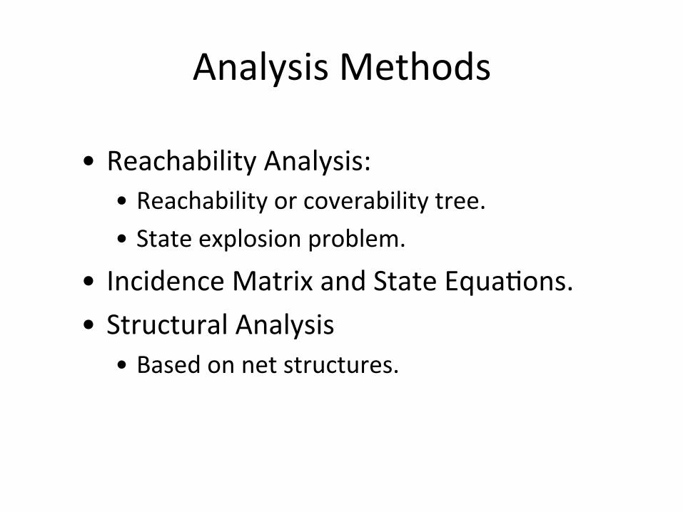
Analysis Methods
• Reachability Analysis: • Reachability or coverability tree. • State explosion problem.
• Incidence Matrix and State Equa4ons. • Structural Analysis
• Based on net structures.

Behavioral proper4es (1) • Proper4es that depend on the ini4al marking • Reachability – Mn is reachable from M0 if exists a sequence of firings that transform M0 into Mn
– reachability is decidable, but exponen4al • Boundedness – a PN is bounded if the number of tokens in each place doesn't exceed a finite number k for any marking reachable from M0
– a PN is safe if it is 1-‐bounded

Behavioral proper4es (2) • Liveness
– a PN is live if, no maler what marking has been reached, it is possible to fire any transi4on with an appropriate firing sequence
– equivalent to deadlock-‐free – strong property, different levels of liveness are defined (L0=dead, L1, L2, L3 and L4=live)
• Reversibility – a PN is reversible if, for each marking M reachable from M0, M0 is reachable from M
– relaxed condi4on: a marking M' is a home state if, for each marking M reachable from M0, M' is reachable from M
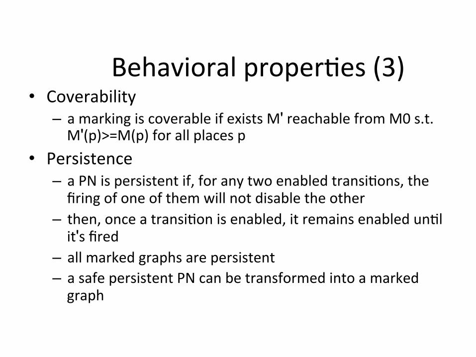
Behavioral proper4es (3) • Coverability – a marking is coverable if exists M' reachable from M0 s.t. M'(p)>=M(p) for all places p
• Persistence – a PN is persistent if, for any two enabled transi4ons, the firing of one of them will not disable the other
– then, once a transi4on is enabled, it remains enabled un4l it's fired
– all marked graphs are persistent – a safe persistent PN can be transformed into a marked graph
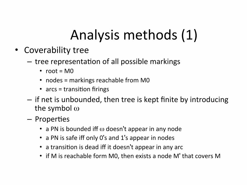
Analysis methods (1) • Coverability tree – tree representa4on of all possible markings
• root = M0 • nodes = markings reachable from M0 • arcs = transi4on firings
– if net is unbounded, then tree is kept finite by introducing the symbol ω
– Proper4es • a PN is bounded iff ω doesn't appear in any node • a PN is safe iff only 0's and 1's appear in nodes • a transi4on is dead iff it doesn't appear in any arc • if M is reachable form M0, then exists a node M' that covers M

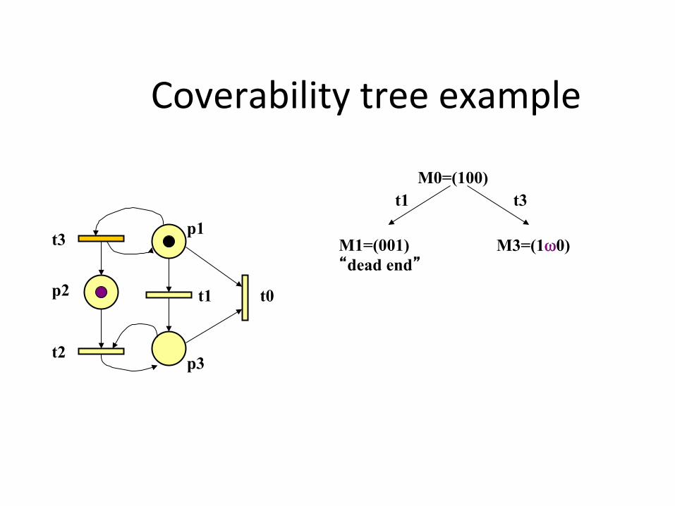
Coverability tree example
t3
p2
t2
p1
t1
p3
t0
M0=(100)

Coverability tree example
t3
p2
t2
p1
t1
p3
t0
M0=(100)
M1=(001) “dead end”
t1
Coverability tree example
t3
p2
t2
p1
t1
p3
t0
M0=(100)
M1=(001) “dead end”
t1 t3
M3=(1ω0)

Coverability tree example
t3
p2
t2
p1
t1
p3
t0
M0=(100)
M1=(001) “dead end”
t1 t3
M3=(1ω0)
t1
M4=(0ω1)

Coverability tree example
t3
p2
t2
p1
t1
p3
t0
M0=(100)
M1=(001) “dead end”
t1 t3
M3=(1ω0)
t1
M4=(0ω1)
t3
M3=(1ω0) “old”

Coverability tree example
t3
p2
t2
p1
t1
p3
t0
M0=(100)
M1=(001) “dead end”
t1 t3
M3=(1ω0)
t1
M4=(0ω1)
t3
M6=(1ω0) “old”
t2
M5=(0ω1) “old”

Coverability tree example
100 M0=(100)
M1=(001) “dead end”
t1 t3
M3=(1ω0)
t1
M4=(0ω1)
t3
M6=(1ω0) “old”
t2
M5=(0ω1) “old”
t1 t3
t1 1ω0 001
0ω1
t3
t2
coverability graph coverability tree

Subclasses of Petri Nets (1) • Ordinary PNs – all arc weights are 1's – same modeling power as general PN, more convenient for analysis but less efficient
• State machine – each transi4on has exactly one input place and exactly one output place
• Marked graph – each place has exactly one input transi4on and exactly one output transi4on
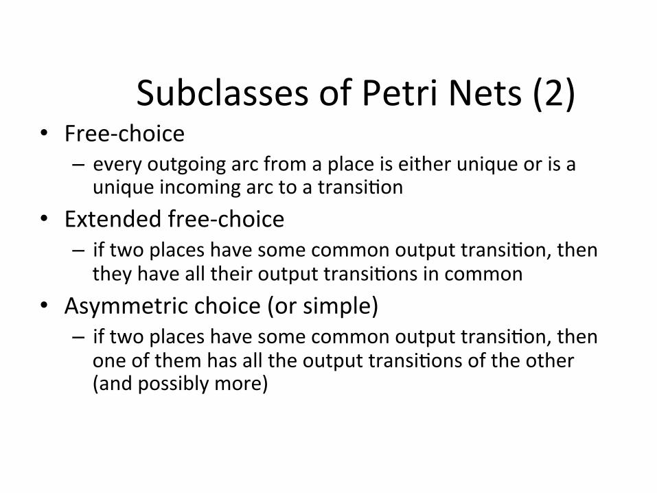
Subclasses of Petri Nets (2) • Free-‐choice – every outgoing arc from a place is either unique or is a unique incoming arc to a transi4on
• Extended free-‐choice – if two places have some common output transi4on, then they have all their output transi4ons in common
• Asymmetric choice (or simple) – if two places have some common output transi4on, then one of them has all the output transi4ons of the other (and possibly more)
Extensions
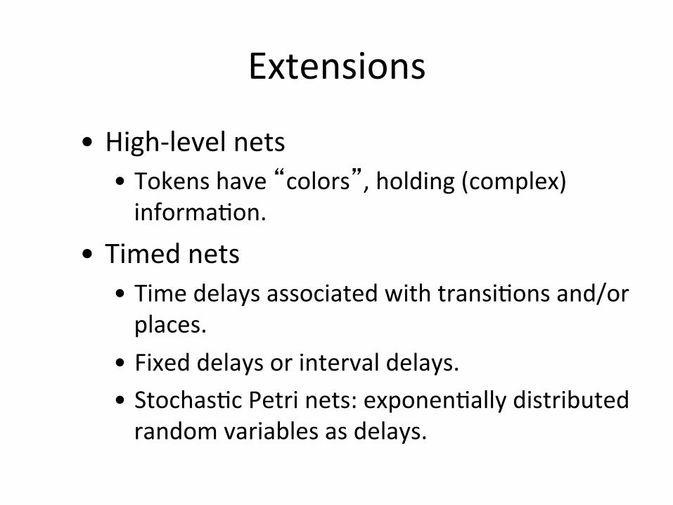
• High-‐level nets • Tokens have “colors”, holding (complex) informa4on.
• Timed nets • Time delays associated with transi4ons and/or places.
• Fixed delays or interval delays. • Stochas4c Petri nets: exponen4ally distributed random variables as delays.

Thanks
• Chris Ling • Gabriel Eirea


