
Finance and Economics Discussion SeriesDivisions of Research & Statistics and Monetary Affairs
Federal Reserve Board, Washington, D.C.
Distance Still Matters: The Information Revolution in SmallBusiness Lending and the Persistent Role of Location, 1993-2003
Kenneth P. Brevoort, John A. Holmes, and John D. Wolken
2010-08
NOTE: Staff working papers in the Finance and Economics Discussion Series (FEDS) are preliminarymaterials circulated to stimulate discussion and critical comment. The analysis and conclusions set forthare those of the authors and do not indicate concurrence by other members of the research staff or theBoard of Governors. References in publications to the Finance and Economics Discussion Series (other thanacknowledgement) should be cleared with the author(s) to protect the tentative character of these papers.

Distance Still Matters: The Information Revolution in Small Business Lending and the Persistent Role of Location,
1993‐2003
Kenneth P. Brevoort* Federal Reserve Board
John A. Holmes
Johns Hopkins University
And
John D. Wolken Federal Reserve Board
December 17, 2009
Abstract: In a seminal article on small business lending, Petersen & Rajan (2002) argue that technological changes have revolutionized small business lending markets, weakening the reliance of small businesses on local lenders and increasing geographic distances between firms and their credit suppliers. While their data only cover through 1993, they conjecture that the pace of change accelerated after 1993. Using the 1993, 1998, and 2003 Surveys of Small Business Finances (SSBFs), we test whether the distance changes identified by Petersen and Rajan continued or accelerated during the following decade. Using a novel application of Oaxaca‐Blinder decomposition, we identify the extent to which specific observable characteristics are associated with distance changes and draw three conclusions. First, while distances increased between 1993 and 1998 at a faster rate than found by Petersen & Rajan, distance increases appear to have halted or possibly reversed between 1998 and 2003. Second, rather than increasing proportionally for all small firms, distance increases were uneven across firms over the decade, with higher credit quality firms and firms with more experienced ownership realizing greater gains in distance than other firms. Finally, distances increased faster at older firms and, regardless of firm age, increases in distance have only affected some product types, primarily those involving asset‐back loans (including mortgages). For relationships that involved the provision of either lines of credit or multiple types of credit, distances increased very little or not at all during the decade. This analysis provides a detailed and nuanced view of how the market for small business credit has evolved during a period of rapid technological change.
* Corresponding author: Ken Brevoort, [email protected]. The opinions expressed in this document
are those of the authors and do not necessarily reflect the views of the Federal Reserve Board or its staff. Ken Brevoort thanks the Center for Economic Research (CentER) and the Department of Finance at Tilburg University for their hospitality while he was working on this paper.

1
Introduction During the past several decades, technological improvements have permitted banks to interact with
customers more efficiently (e.g., online banking and automated teller machines) and to measure and
manage risk more effectively (e.g., credit scoring). At the same time, deregulation has reduced
restrictions on branching activity (both intrastate and interstate) and, through federal preemption,
increased the ability of banks in one state to offer financial services in other states free from additional
regulatory burden. As a consequence of these and other changes, the banking marketplace in the U.S.
has been substantially altered as bank consolidation has increased the size and geographic scope of
banks (Critchfield, et al, 2004; DeYoung, et al., 2004). While the existence of these changes has been
undeniable in most aspects of banking, in small business lending, where borrowers have historically
relied more on soft information and relationship lending for credit, the extent to which the same
technological changes have expanded the geographic reach of lenders has remained in dispute.
In a seminal article on small business lending, Petersen and Rajan (2002) argue that
technological changes have revolutionized small business lending by expanding access to credit from
more distant suppliers, thereby breaking “the tyranny of distance” in small business lending. The
authors draw two conclusions from their data analysis. First, the physical distance between small
businesses and their lenders grew steadily (about 3.4 percent per year) between 1973 and 1993.
Second, fewer small businesses list their primary means of interacting with their lenders as being in
person. These conclusions are drawn from an analysis of a “synthetic panel” that the authors construct
from the 1993 Survey of Small Business Finances (SSBF) to represent small business lending activity from
1973 to 1993.1 While the data used to support their conclusions only cover through 1993, Petersen and
Rajan conjecture, based upon conversations with industry experts and evidence in other studies,2 that
not only has the trend towards longer physical distances between small businesses and their lenders
been steady, but “if anything the trend has accelerated since 1993” (Petersen and Rajan, 2002, p. 2534).
The 2003 SSBF provides an opportunity to test this conjecture. Using these data, we revisit the
issues raised by Petersen and Rajan (2002) to determine the extent to which increases in the physical
distance between small businesses and their lenders have continued or possibly accelerated over the
subsequent decade. Rather than constructing a synthetic panel from a single wave of the SSBF, we
1 Petersen and Rajan (2002) also utilize the 1988 SSBF as a robustness check. The same method of creating a
synthetic panel from each cross section of SSBF data is employed for the 1988 data. 2 The authors do not provide citations to these other studies.

2
compare the results from the 1993, 1998, and 2003 SSBFs to examine how distances between small
firms and their suppliers of credit evolved over time. These surveys provide the most comprehensive
look at the financing of small businesses available over this time period and afford the best picture of
how distances changed across all types of financial institutions for a nationally representative sample of
small business borrowers. Our analysis utilizes Oaxaca‐Blinder decomposition in a novel way to examine
how distances changed across firms with differing characteristics. While we are unaware of any
previous studies that have used Oaxaca‐Blinder decomposition to study the effects of technological
change over time, this methodology is well suited to identify those firm characteristics that are the most
related to changes in distance over the decade.
Our analysis leads us to three conclusions about how distances between small businesses and
their suppliers of credit changed over the 1993 to 2003 decade. First, while distances increased during
the first five years – indeed, at a faster rate than that found by Petersen and Rajan (2002) – the
increases appear to have halted, or possibly even reversed somewhat, between 1998 and 2003. Second,
rather than increasing proportionally across the board for all small firms, increases in distance played
out unevenly across firms over the decade, with higher credit quality firms and firms with more
experienced ownership realizing greater gains in distance than other firms. Finally, distances have
increased faster at older firms than at younger firms, and, for all firm age groups, increases in distance
have only affected some product types, primarily those involving asset‐backed loans (including
mortgages). For relationships that involved the provision of either lines of credit or multiple types of
credit, distances increased very little or not at all during the decade.
Our results have important implications for understanding how the allocation of credit to small
businesses is evolving over time. They also have important implications for antitrust policy, particularly
in evaluating the likely competitive effects of proposed bank mergers. If the increase in distances over
which small businesses and suppliers of credit interact had continued to increase over the decade, then
this may have suggested that small firms are less dependent upon local lenders as sources of credit.
Such a finding would mitigate concerns that a merger between financial institutions in the same local
market might allow the merged institution to extract rents from small businesses that are captive to
local suppliers of credit. Our analysis suggests that the provision of bank credit remains largely local,
and therefore that merger enforcement ought to remain vigilant.

3
The plan for the paper is as follows. The next section provides a brief review of empirical studies
on how the distance between small businesses and their sources of credit has changed in recent years.
The following section describes the SSBF data and presents univariate statistics on how distances
changed across the three survey years. The subsequent section presents the results of our multivariate
analysis of distance changes, which controls for a variety of firm‐ and relationship‐specific
characteristics. This section also details our use of Oaxaca‐Blinder decomposition and presents
documents our simulations of distance changes across different types of firms. The final section
discusses our results and the conclusions that we draw from them.
Literature Review
The reasons why distance, or more specifically, geographic proximity, should matter in small business
lending can be traced to transaction costs incurred by both borrowers and lenders. Brevoort and
Wolken (2009) provide a detailed review of the literature on why distance should matter to banking and
how the transaction costs that give rise to the importance of distance may have been impacted by
technological and regulatory changes in the recent past. We follow here with a limited review of
empirical studies on distance in small business lending.
Empirically, the relationship between physical proximity and small business lending patterns has
been well documented. Using the 1993 SSBF, Kwast, Starr‐McCluer, and Wolken (1997) find that 92.4
percent of small businesses use a depository institution that is within 30 miles of their main office. Data
from the 2001 Credit, Banks, and Small Business Survey, conducted by the National Federation of
Independent Businesses and detailed by Scott (2003), indicate that the average travel time between a
small business and its primary financial institution was 9.5 minutes. Using this same data source, Amel
and Brevoort (2005) estimate that 90 percent of small businesses look for banking services within 14.8
miles of the firm’s location.
The first paper to examine how the geographic distance between small businesses and their
lenders is changing over time was by Petersen and Rajan (2002), who as mentioned earlier use the 1993
SSBF to construct a synthetic panel based upon the year in which the relationship between the small
business and its lender began. While the data extend farther back in time, the authors exclude those
lending relationships that began prior to 1973 and focus on changes in the pattern of lending over the
next two decades, from 1973 to 1993. Petersen and Rajan (2002) conclude that the distance between

4
small firms and their lenders has been increasing by 3.4 percent per year, an increase that they attribute
to increases in bank productivity brought about by technological advances.
Several empirical studies followed examining how distances between small businesses and their
lenders are changing over time. Wolken and Rohde (2002) used the 1993 and 1998 SSBFs and Brevoort
and Wolken (2009) used the 1993, 1998, and 2003 SSBFs to examine univariate distance changes across
surveys. Wolken and Rohde (2002) find that while mean distances had grown at a quicker rate than
predicted by Petersen and Rajan (2002), an annual rate of over 15 percent, that median distances had
only changed slightly from 9 miles in 1993 to 10 miles in 1998. The difference between changes in mean
and median distances suggests that changes in the small business lending marketplace during that time
period largely affected the upper tail of the distance distribution. Brevoort and Wolken (2009) find
similar changes between 1993 and 1998, but supplement this with results that show that mean
distances generally declined between 1998 and 2003.
Another series of papers has examined this issue using data from the Community Reinvestment
Act (CRA). The CRA data provide annual information on the number and dollar amount of small business
loans made by depository institutions, by census tract. When combined with data on bank branch
locations from the Summary of Deposits data, CRA data can be used to examine how the geographic
distribution of small business loans originated at depository institutions changed relative to their branch
networks over time. Studies using this data have either focused on how lending changed to geographic
areas at different distances from the bank’s branch network, or how out‐of‐market lending (defined as
loans to geographic areas in which the depository institution has no branch presence) has changed.
These studies include Hannan (2003), Brevoort and Hannan (2006), Brevoort (2008), and Laderman
(2008). In general, studies based upon CRA data (which cover years as late as 2003) have shown little
evidence that depository institutions are extending credit at greater distances. To the extent that out‐
of‐market lending activity has increased, it has largely been confined to particularly small loans – loans
with average balances small enough to resemble credit card loans.
Studies of changing distances in small business lending have also been conducted using data
from the U.S. Small Business Administration’s (SBA’s) 7(a) Loan Program. This program targets small
businesses that have been unable to obtain financing from conventional sources. Loans made under
this program generally carry a government guarantee for between 50 and 85 percent of the outstanding
loan balance. According to the U.S. Government Accountability Office (2007) this program accounts for

5
an estimated 1.3 percent of small business loans and 4.1 percent of outstanding small business loan
dollars for loans under $1 million in 2005. Papers using this data include DeYoung, Glennon, and Nigro
(2006), DeYoung, et al. (2008), and DeYoung, et al. (2007b). These studies have generally found that
distances grew between 1984 and 2001, with larger increases at banks that had adopted credit scoring
by the time of a 1998 Atlanta Fed survey. While it is not possible to identify a treatment effect of credit
scoring in these studies, the results are consistent with the increases in mean distances observed in the
previously mentioned literature and with the notion that increases in distance have not played out
equally across all lenders.3
These studies present differing views of what has happened to the geographic distances
between small firms and their lenders. For the studies involving data from the CRA or SBA, the studies
represent only subsets of the small business lending market. Additionally, these studies collectively
provide very little evidence about how changes in distance over time may have played out differently
over time. Instead, each (with few exceptions) treats any changes in distance over time as average
effects that are felt by all firms uniformly or proportionally. In this study, we supplement these studies
by examining a dataset that is nationally representative of the financing of all small firms and conduct a
careful examination of how distance changes may have played out across firms with different
characteristics.
Data and Univariate Analysis
Since its inception, the Survey of Small Business Finances (SSBF) has provided the most comprehensive
picture available of the financial dealings of small businesses. The SSBF has several advantages over
other data sets in examining distance changes in small business lending. Unlike regulatory data or data
from a single banking institution and its customers, the SSBF surveys small businesses directly and
obtains a nationally representative dataset of small businesses’ financial relationships and the services
that they use. The data provide an inventory of all financial services and suppliers used by each firm,
and consequently creditors other than banks can be examined. While studies utilizing data from
individual banks or the CRA typically have little information available on the firm, the SSBF contains a
broad set of firm and owner characteristics.
3 For additional information on the role of credit scoring in small business lending, see Frame, et al (1996);
Cowan and Cowan (2006); and Berger, et al (2009).

6
In the SSBF, firms are asked to identify and provide information about the institutions from
which they received financial services. This information can also be matched to other data sources to
obtain additional characteristics of the financial institution or the market or geographic area in which
the firm is headquartered. The firm is also asked to report both the location of the office or branch of
the financial institution used most frequently, and the distance between the firm’s headquarters and
that office. When the firm does not know the distance, the location of the financial service provider is
used to calculate the distance between the firm’s main office and each of its suppliers.4 These data
permit an examination of how the geographic relationship between a small business and its suppliers of
credit varies by institution and product type, and how these geographic relationships have changed over
the 1993‐2003 decade.
Table 1 provides detail on four different distance measures for each of the three survey years,
broken down by financial institution type and the product being supplied.5 As with the rest of the paper,
the unit of observation used in constructing these numbers is the firm‐credit supplier pair and only
those firms with an existing credit relationship (i.e., that had a loan, line of credit, or capital lease) are
included. 6 In addition to mean and median distances, the percentage of relationships that are
conducted with nonlocal suppliers (defined as distances greater than 30 miles) and the mean of the log
of one plus distance are included. Table 2 provides p‐values for tests of the equality of means between
each of the survey years (1993 vs. 1998, 1998 vs. 2003, and 1993 vs. 2003) for each of these distance
measures, except median distance. The unit of observation used in this table, and in the study more
broadly, is the credit relationship between a firm and its financial institution, so that the means and
medians reported in the table represent relationship distances.
4During the 1993, 1998, and 2003 surveys, respondents were asked the following: “Think of the office or
branch of (NAME) that the firm used most frequently. (i) Approximately how many miles from the main office of the firm is this office or branch? (ii) What was the most frequent method of conducting business with this office or branch?” Firms are also asked to provide the address and zip code for this branch or office. For additional details, see the questionnaire or codebook for the surveys at Board of Governors of the Federal Reserve (2008) at http://www.federalreserve.gov/pubs/oss/oss3/nssbftoc.htm.
5 The sample design in all survey years was a nonproportional stratified random sample with oversampling of larger small businesses. All statistics in this paper are weighted with survey weights that reflect differences in sample selection probabilities and response rates. As a result, statistics represent population estimates.
6 The descriptive statistics presented here are similar to those in Brevoort and Wolken (2009). However, this study focuses exclusively on firms using loans, lines of credit, or capital leases whereas the earlier study imposed no such restriction.

7
The four unconditional distance measures shown in table 1 each provide a similar picture of how
distances evolved over the decade. Relationships between small business firms and their suppliers of
credit were conducted at greater distance in 2003 than they had been in 1993. Over the decade, the
mean distance between small businesses and their providers of credit increased by 70 miles, a change
that was significant at the 1 percent level. The pattern over the decade, however, was not monotonic.
From 1993 to 1998, mean distances increased by over 130 miles, only to decrease five years later by 60
miles. Both of these changes are significant at the 1 percent level. A similar pattern holds for the mean
log distance measure, though the decline from 1998 to 2003 is not statistically significant. In contrast,
both the median distance and the percent nonlocal measures suggest that distances increased during
the decade, though again the change from 1998 to 2003 was not statistically significant for percent
nonlocal.
Distances between small businesses and their credit suppliers vary widely by the type of
institution supplying credit and the product type. This is true both for distances at the start of the
decade and for the way changes in distance occurred during the decade. In particular, distances
changed less for relationships with depository institutions than for those with nondepositories. This
pattern holds across all four distance measures for each of the three years of the SSBF. However,
distances changed over the decade for these two institutions types very differently. At depository
institutions, the changes were very minor. In contrast, there is a very clear trend of distances increasing
in the early part of the decade and decreasing thereafter for nondepositories. The 5‐year changes at
nondepositories are significant at the 1 percent level in each case.
Distances can also be examined based upon the type of credit product being supplied. Four
distinct types of credit are identified: lines of credit, mortgage loans, asset‐backed loans (including
motor vehicle loans, equipment loans, and capital leases), and all other loans. Relationships involving
the provision of more than one of these are classified as “bundle relationships.” Bundle relationships
may allow economies of scale on borrowers’ transaction costs to be achieved if all loans are at the same
lender, and hence may be more likely to be obtained from local lenders. The remaining relationships
involve only a single type of credit and are classified on this basis as lines of credit only, mortgages only,
asset‐backed loans only, and other loans only. These five credit products are mutually exclusive and
comprise the products depicted in tables 1 and 2.

8
There are substantial differences in relationship distances across product types. Bundle
relationships are conducted at much shorter distances than relationships involving a single product.
There is also little evidence that distances for bundle relationships increased over the decade, as none of
the distance changes are significant at the 5 percent level. Lines of credit were the next most proximate
credit product. For lines of credit, the mean distance increased significantly over the decade; other lines
of credit distance measures were not statistically different over the decade.
The largest relationship distances are observed for relationships in which only asset‐backed
loans are extended. Asset‐backed‐loan‐only relationships are the most commonly observed relationship
type and show the clearest pattern of distances increasing during the early portion of the decade and
declining thereafter (a pattern observed for all four distance measures, as shown in table 1).
Nevertheless, these relationships also experienced the largest increases in distance over the decade as a
whole. For relationships involving the provision of only mortgages or only other loans, the pattern is
somewhat different. While distances for these products increased over the decade, the increase
appears to have occurred primarily between 1998 and 2003 (though this pattern is not evident in the
mean distance measure for mortgages).
These results suggest that while distances were generally higher in 2003 than 10 years earlier, a
portion of the substantial increase in mean distance between 1993 and 1998 was erased in the latter
half of the decade as mean distances declined between 1998 and 2003, though these changes were not
always statistically significant.
In the following section, we explore how distances have changed over the decade using
multivariate methods. Our analysis proceeds in three stages. In the first stage, we conduct a reduced
form analysis of distance in each of the three waves of the SSBF individually. We then examine distance
over time in a single pooled regression that combines all three survey years. The second stage utilizes
Oaxaca‐Blinder decomposition to examine how changes in distance observed over the decade can be
attributed to changes in the distribution of firm characteristics, or to changes in technology or other
unobserved factors that may have altered the relationship between individual firm characteristics and
distance. This decomposition is used to identify those dimensions of firm characteristic space along
which the changes in distance were the least uniform. Finally, the third stage of our analysis uses
simulation methods to examine how distances changed at different types of small businesses.
9
STAGE 1: REDUCED FORM ANALYSIS OF RELATONSHIP DISTANCES IN 1993, 1998, AND 2003
The Model As discussed in detail in Brevoort & Wolken (2009), the importance of geographic proximity in small
business credit markets (as in banking in general) derives from transaction costs associated with the
provision of credit. Several of these transaction costs may increase with distance, including loan
production costs for lenders (e.g., solicitation, underwriting, and loan monitoring costs) and borrowers
(e.g., costs of search and information exchange), or costs related to the increased credit risk associated
with dealing with distant borrowers about whom lenders may have less information than their closer
competitors. Distance‐related costs make credit extensions from distant lenders relatively more
expensive than extensions from nearby lenders. Over time, distance related costs may have decreased
due to technological developments.
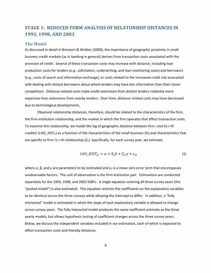
Observed relationship distances, therefore, should be related to the characteristics of the firm,
the firm‐institution relationship, and the market in which the firm operates that affect transaction costs.
To examine this relationship, we model the log of geographic distance between firm i and its r‐th
creditor (LOG_DISTir) as a function of the characteristics of the small business (Xi) and characteristics that
are specific to firm i's r‐th relationship (Zir). Specifically, for each survey year, we estimate
_ (1)
where , β, and γ are parameters to be estimated and єir is a mean zero error term that encompasses
unobservable factors. The unit of observation is the firm‐institution pair. Estimations are conducted
separately for the 1993, 1998, and 2003 SSBFs. A single equation covering all three survey years (the
“pooled model”) is also estimated. This equation restricts the coefficients on the explanatory variables
to be identical across the three surveys while allowing the intercept to differ. In addition, a “fully
interacted” model is estimated in which the slope of each explanatory variable is allowed to change
across survey years. The fully interacted model produces the same coefficient estimate as the three
yearly models, but allows hypothesis testing of coefficient changes across the three survey years.
Below, we discuss the independent variables included in our estimation, each of which is expected to
affect transaction costs and thereby distances.

10
Firmspecific characteristics (Xi). Firm‐specific characteristics that may impact distance‐related transaction costs incurred by the firm or
its lenders in extending credit are included in the estimation. We segment these characteristics into five
groups that include creditworthiness, opacity, management, industry, and local credit market
characteristics. Table 3 provides means for each of these variables for each of the three survey years
and for the pooled sample.
Creditworthiness: Characteristics in this group relate to a lender’s likely evaluation of the firm’s
credit risk. Since lenders often rely on characteristics of both the business and the business’s owner(s)
in evaluating credit risk, we include measures of both the owner and the firm. Specifically, as measures
of each firm’s credit quality we include the firm’s Dun & Bradstreet credit score (CSPCT), which is a rank
ordering of the firm’s credit risk based solely upon the characteristics of the business itself. We also
include an indicator variable (BADHIS) that is equal to 1 if the business owner or firm has recently been
delinquent on either business or personal credit obligations, has filed personal or business bankruptcy,
or has judgments against the firm or its owner.7 The firm’s credit quality should be positively associated
with CSPCT and negatively associated with BADHIS. As discussed in the Opacity section below, the
impact of credit quality on distance is theoretically ambiguous.
Opacity: Related to a firm’s credit quality is the extent to which its true quality is opaque (or
conversely transparent) to prospective lenders. Variables included in the model to capture the extent of
information opacity include the firm’s age (LOG_ZFAGE) and asset size (LOG_ASSETS). Both size and age
have been used extensively in the literature as measures of information opacity (Petersen and Rajan,
1995; Berger and Udell, 1998; Petersen and Rajan, 2002; Scott and Dunkelberg, 2003; Hyytinen and
Pajarinen, 2007; and Black, 2009), with older and larger firms believed to be less opaque. At the same
time, however, both firm age and asset size may also be related to the firm’s credit quality or the firm’s
demand for credit.
7 The SSBF includes several measures of self‐reported credit history including firm and principal owner
bankruptcy in the last seven years, late payments (late 60 days or more three or more times in the past three years) and judgments. Individual indicators for each of these six types of credit events were included individually. However, many of these (bankruptcy and judgments) are fairly rare in the population of small businesses and individually the coefficients were generally insignificant. Consequently, a single indicator was utilized to reflect the self‐reported credit history.

11
Since incorporation may affect the type and amount of information that the firm must make
available, an indicator of whether the firm was organized as a corporation (CORP) is included as a
measure of opacity. However, incorporation may also have other effects, particularly if the limited
liability that goes along with incorporation increases distance‐related transaction costs. The final
measure of information opacity is an indicator variable for whether the firm’s respondent used financial
records in completing the SSBF questionnaire (RECORDS). This variable has been used previously as a
measure of information transparency (Petersen and Rajan, 2002). A firm that used detailed financial
records to complete the survey should be better able to use those records to accurately convey its credit
quality to prospective lenders.
Both higher credit quality and higher information transparency should make prospective
borrowers more attractive to lenders. However, it is unclear ex ante how these measures will affect
average distances. On one hand, suppliers or lenders may only be willing to extend credit to firms that
they can verify are low risk (which would be those creditworthy firms that are sufficiently transparent).
Since the ability of a lender to measure credit risk may decrease with distance, distant lenders may be
more cautious in extending credit as they seek to minimize adverse selection. Consequently, one might
expect high quality firms to obtain credit at greater distances than riskier firms.
On the other hand, while more transparent and creditworthy firms may be better able to obtain
funding from more distant lenders, they will also be more able to obtain funding locally. If small
business borrowers incur distance‐related transaction costs, then these firms may prefer local lenders,
other things equal. In this case, high quality firms will be able to obtain credit from proximate lenders,
while lower quality firms may have to expand the radius in which they search for sources of credit, if
they cannot receive credit from local lenders. In this case, we would expect higher credit quality and
transparency to be associated with shorter relationship distances. The impact of credit quality and
transparency on average distances is theoretically ambiguous.
Management: Small firms with professional or more experienced management may be more
aware of financing alternatives or have a broader network of financial contacts to call upon.
Consequently, one might expect characteristics of a firm's management to be related to distance. The
model includes two firm management characteristics: the years of experience of the firm's principal
owner (LOG_OWN1_EXP) and an indicator variable for whether the firm's owner(s) is (are) also its

12
manager(s) (MGR). We expect the coefficient on LOG_OWN1_EXP to have a positive sign and the
coefficient on MGR to be negative.
Industry: A firm’s industry may be related to its demand for credit, the type of creditors it likely
maintains relationships with, and the willingness of lenders to extend credit to the firm. To capture
industry‐related effects, the model includes control variables for the firm’s primary industry as indicated
by eight industry dummies based on the firm’s 4‐digit SIC code.8
Local credit market characteristics: More competitive and larger banking markets may provide a
greater array of in‐market credit alternatives to firms. The estimations include, as a measure of the
concentration of the local banking market, the Hirschmann‐Herfinadahl Index (HERF) for the banking
market in which the firm’s headquarters is located. Firms in less concentrated (or more competitive)
markets are expected to have less of a need for sources of credit outside of their local market. As a
result, this measure of concentration is expected to be positively related to distance. Additionally, we
include an indicator variable that equals 1 if the firm was headquartered in a Metropolitan Statistical
Area (MSA) and, because MSA and HERF are likely to be highly correlated, an interaction between MSA
and HERF (MSA*HERF). Since firms in MSAs should have more local options for credit available to them,
we expect MSA to be negatively related to distance. Estimations also include the log of the number of
bank branches per square mile in the firm’s local market (DENSITY). Firms with more bank branches
nearby may be more aware of or have access to more local funding opportunities and consequently may
be more likely to obtain credit locally. We expect DENSITY to be negatively related to distance.
Firms with operations in multiple markets may have direct access to more than one local credit
market, whereas firms operating in a single geographic area typically have access to a single local
market. Since distance is measured from the office or branch of the lender used most often by the firm
to the firm's headquarter location, multimarket firms may have higher observed distances in the data.
To account for this possibility, indicator variables for whether the firm has offices outside of the local
banking market (NONMKT) and whether the sales area of the firm is national (NATIONAL) as opposed to
regional or local are included, with the expectation that distances are larger for these types of firms.
8 The industries include mining and construction (SIC<2000), manufacturing (2000=SIC<4000), transportation
(4000=SIC<5000), wholesale trade (5000=SIC<5200), retail trade (5200=SIC<6000), insurance and real estate excluding depository institutions (6000=SIC<7000), personal services (7000=SIC<8000), and professional services (8000=SIC<9000).

13
Relationshipspecific characteristics (Zi) The model also includes characteristics that are specific to the firm‐institution relationship. These
characteristics vary not only across firms, but also across the different credit relationships that a firm
maintains. Relationship‐specific characteristics fall into three broad categories: financial institution
type, product characteristics, and length of relationship.
Financial Institution Type: A financial institution’s willingness to extend credit over long
distances may be affected by its informational advantages (if any) as well as the regulatory incentives to
focus on local or less risky lending. Depository institutions (commercial banks, savings banks, savings
and loan associations and credit unions) may possess different information advantages and regulatory
incentives than nondepository institutions. Information advantages may be related to the unique ability
of depository institutions to offer transactions accounts, which most nondepository institutions are not
able to offer. Depository institutions that offer such products may glean information from the cash‐flow
information associated with these accounts. Regulatory incentives include, for example, the Community
Reinvestment Act. This Act establishes that depository institutions in the United States have an
affirmative obligation to meet the credit needs of the local communities from which they draw their
deposits. Bank and thrift regulators routinely examine the lending practices of depository institutions to
evaluate whether they are meeting these obligations. These regulations, as well as regulations related
to safety and soundness, the unique products offered by depository institutions, and the information
generated from these product offerings suggest that such policies may provide depository institutions
with a greater incentive to focus on local lending activities. To account for such possible differences, the
estimations include an indicator variable (DEPOSIT) that takes on a value of 1 if the relationship is with a
depository institution and zero otherwise.
Product characteristics: The type of product being provided may also affect relationship
distances. For example, some loans are collateralized with items that have active secondary markets –
asset‐backed loans such as equipment, automobiles, or other fixed assets – and hence may require less
monitoring than other types of loans such as lines of credit or term loans which often have covenants or
collateral which need to be examined periodically. To account for differences in product characteristics,
lending relationships were divided into the five product types described in the previous section.
Specifically, each lending relationship is classified according to whether the relationship involved the
provision of lines of credit only (LOC), mortgages only (MORT), asset‐backed loans only (ASSET), other

14
loans only (OTHLN), or a bundle of multiple loan types (BUNDLE). Asset‐backed loan only relationships
are used as the omitted category. Because asset‐backed loans often involve well‐defined secondary
markets and are collateralized by the item being financed, we expect other loan types to be associated
with smaller distances than asset‐backed loans. In particular, bundle relationships may allow economies
of scale on borrowers’ transaction costs to be achieved if all loans are at the same lender, and hence
may be more likely to be obtained from local lenders.
The model also includes an indicator variable denoting whether the loan involved the pledging
of collateral (COLLAT). Since collateral can limit the amount of loss incurred by a lender in the case of
default, a collateralized loan may be less risky and consequently lenders may be more able to profitably
make loans that involve collateral. If more distant borrowers are relatively riskier, then one might
expect the provision of collateral to increase the willingness of lenders to extend credit at greater
distances.
Finally, the last product characteristic variable is an indicator variable (CHECK), which denotes
whether the relationship also involved the provision of a checking account. Providing checking account
services may help a lender monitor small business loans (Norden and Weber, 2008), which could reduce
transaction costs associated with loan monitoring. However, if the provision of checking services itself
entails transaction costs that are related to distance, then this would provide a competitive advantage
to more proximate lenders. Moreover, customers of multiple products (checking and one or more
loans) may experience economies of scope in the transaction costs associated with their institution, and
hence those relationships are likely associated with smaller distances.
Length of Relationship: The importance of ongoing relationships in the provision of small
business credit is well established (Petersen and Rajan, 1994; Boot, 2000; Berger and Udell, 2002). If
relationship lending confers soft information through personal interactions and site visits that occur as
part of loan underwriting and monitoring, then geographic proximity may increase the profitability of
relationship lending for local lenders. Consequently, we would expect longer relationships to involve
closer firms and include a variable measuring the log of the number of years for which the relationship
has existed (LOG_REL). The length of relationship may also involve a certain amount of “path
dependence” in that lending relationships observed in the survey may reflect decisions made in previous
years. If over time small business lending has moved away from relationship lending towards more
transaction‐based lending technologies, then one would expect to observe shorter relationships that

15
were entirely based upon more recent considerations (such as more recent lending technologies) in the
later surveys. Observed distances would therefore more fully reflect lending conditions at the time of
the survey.
Our treatment of the length of relationship variable is one of the substantive differences
between the analysis undertaken here and the study by Petersen & Rajan (2002). In their paper,
Petersen & Rajan identify distance trends from differences in this length of relationship variable. Using
the 1993 SSBF, Petersen & Rajan identify the change in distance between 1990 and 1991 as the
difference in distances between relationships that had been in existence for three years in 1993 and
those that had been in existence for two years, after controlling for other factors. For reasons that are
discussed in detail in Appendix B, we believe that this treatment suffers from serious selection biases
that overstate the changes in distance over time. Instead of the approach taken by Petersen & Rajan,
we control for the length of relationship and examine how distances changed across the three surveys.
Our identification of distance changes over time, therefore, comes from comparing the mean distances
of relationships begun n years ago and reported in 1993 with the mean distances for n‐year‐old
relationships reported in the 1998 and 2003 SSBFs, while controlling for other factors. This method
allows us to account for any path dependence in relationship distances without sample selection bias.
These firm‐specific and relationship‐specific characteristics constitute the set of explanatory
variables used to examine how distances between small firms and their lenders changed over the 1993‐
2003 decade.
Regression Results The results of the regressions of LOG_DIST on the set of firm‐ and relationship‐specific variables are
presented in table 4. The first three columns report the coefficients from the estimation of equation (1)
for each of the three survey years separately. The fourth column provides the results from the
estimation of the pooled model. Results from the fully interacted model, which are identical to those of
the three yearly estimations, are not presented in the tables. However, the variance‐covariance matrix
from this model is used to calculate the test statistics for the hypothesis tests across survey years
discussed in the text.9 The p‐values from one set of tests, that the coefficients on an individual variable
9 Algebraically, the coefficient estimates for the fully‐interacted (with survey year) pooled model are identical to

16
are constant across the three survey years, are provided in the Memo column of table 4. Additionally,
table 5 provides p‐values for tests of the joint significance of the coefficients on the variables in each
characteristic group for the three individual year estimations and for the pooled model.
The estimation results across the three survey years and for the pooled estimation point to
several explanatory variables that are consistently and significantly related to relationship distances. In
particular, three explanatory variables, LOG_REL, DEPOSIT, and CHECK, stand out as being significantly
related to distance at the 1 percent level in all four estimated equations. The coefficients on each of
these three variables are negative, which indicates that credit relationships involving depository
institutions, the provision of checking accounts, or those in existence for longer periods tend to be
transacted at shorter distances. Using the estimated coefficients from the pooled estimation as an
example, relationships involving depository institutions were 76.1 percent closer than relationships with
other types of institutions. Similarly, if the relationship involved the provision of checking account
services, then distances were 77.4 percent closer than relationships that did not involve these services.
Finally, a 1‐percentage point increase in the length of relationship (which at the sample means would
translate into an increase of approximately three weeks) is associated with a decline in distance of about
0.2 percent.10
The coefficients on variables representing local market characteristics are generally of
consistent sign across the estimated equations and each is significant at the 5 percent level in both the
2003 and the pooled models. Distance increases with concentration (HERF) in rural markets, but the
effect is attenuated in urban (MSA) areas. As expected, distances decrease as the bank branch density
(DENSITY) rises, but increases for those firms that operate nationally (NATIONAL) or have offices located
outside of the headquarter’s market (NONMKT). The fact that all six variables are significant in 2003 and
only sporadically significant in earlier years suggests that the importance of local banking market
characteristics is a more recent phenomenon. While the coefficients on some of these variables
remained relatively constant across the three individual year estimations (such as NONMKT), the
magnitude of the coefficients on other variables (i.e., DENSITY and MSA*HERF) increased substantially.
the coefficient estimates obtained from estimating the same equation independently for each of the survey years. However, the fully‐interacted pooled model allows a variance‐covariance matrix to be calculated that permits hypothesis testing across coefficients in different survey years, as well as testing the hypothesis that the three equations have identical coefficients. This latter hypothesis is rejected at the 1 percent level of confidence.
10 For a detailed explanation of how percentage changes in distance were calculated, see Appendix A.

17
Nevertheless, for each of the variables in this group, we are unable to reject the hypothesis that its
coefficient remained constant across the three individual year estimations.
Other explanatory variables appear to be related to observed distances, but without the
consistency across the four estimations observed for the variables already discussed. This is consistent
with an evolving small business lending market in which technological changes are altering the distance‐
related transaction costs associated with the extension of small business credit. The relationship
between distance and those variables that are related to the transaction costs that have been affected
by technological change should change as technology changes.
One of the most interesting variables in this context is the firm’s credit score, CSPCT. Credit
score is negatively associated with distance at the 1 percent level in 1993, but has almost no association
with distance in the later two surveys. This suggests that in 1993, lower credit quality firms were more
likely to obtain credit from distant suppliers than were higher quality firms. A similar result is found for
the other credit quality proxy, BADHIS, which indicates whether or not the firm’s owner had a history of
bad credit. This variable is not significant in any of the three years (or in the pooled model), though the
coefficient is positive in the first two years (which is again consistent with lower quality firms getting
credit from more distant suppliers) and close to zero in 2003. The implication is that at the start of the
decade being examined in this study, it was the lower quality firms who went farther to obtain credit
while by the middle of the decade, low and high quality firms were about equally likely to obtain credit
from distant suppliers, holding other factors constant.
The importance of owner experience also appears to have changed over the decade.
Coefficients on LOG_OWN1EXP were small and insignificant in the 1993 and 1998 estimations, but
positive and significant at the 10 percent level in 2003. The positive effect of owner experience suggests
that firms with more experienced owners are more likely to obtain credit from distant suppliers, though
this appears to be a relatively recent phenomenon. We can reject the hypothesis that the relationship
between LOG_OWN1EXP and distance was constant across the three survey years at the 10 percent
level. The other variable representing the firm’s management, MGR, was insignificant in all four
estimations.
As discussed earlier, information transparency is related to credit quality, though the
coefficients on variables in this group exhibit little evidence of change over the decade. Firm asset size,
LOG_ASSETS, and the records indicator, RECORDS, each have consistent positive signs across the

18
estimations, suggesting that transparent firms are likely to obtain credit at greater distances than
opaque firms. While both of these variables are sporadically significant, using the fully‐interacted
model, we are unable to reject the hypothesis that the coefficients on either LOG_ASSETS or RECORDS
were constant over the decade. Coefficients on the other two variables in this group, LOG_FAGE and
CORP, were small and insignificantly different from zero in each of the four estimations.
Change in Distance over Time The estimation of the pooled model (table 4, column 4) allows direct inferences to be made about how
distances changed across the three survey years. The results from this model show that, after
controlling for other factors, distances followed the same pattern over time in this multivariate setting
as they did in the univariate setting described earlier.
Focusing on the intercept and survey year dummies, distances from the 1998 survey were
significantly larger (at the 1 percent level) than those from 1993. As implied by the coefficient on
D1998, distances were 40 percent higher in 1998 than they had been in 1993. This is equivalent to an
average annual growth rate of 7 percent, which is considerably higher than the 3.4 percent rate
reported by Petersen and Rajan (2002).11 This result is consistent with their speculation that the rate of
change in distance had accelerated after 1993.
During the next five years, however, distances appear to have declined. Specifically, after
controlling for other factors, distances in 2003 were about 13 percent lower than they had been in 1998.
This decline is statistically significant at the 5 percent level (p‐value=0.0136, not shown in tables). As a
result of this decline, distances over the decade as a whole were approximately 21 percent higher than
they had been in 1993. This corresponds to an average annual growth rate over the decade of 1.9
percent. This is slower than the 3.4 percent rate of increase found by Petersen and Rajan (2002).
The results from the pooled model, however, rely on the strong assumption that the underlying
relationship between the explanatory variables and distance remained constant over the decade. As we
saw in the preceding section, coefficient values changed significantly over this period and we are able to
reject the hypothesis that the coefficients on the explanatory variables (other than the survey year
indicators) are identical across the three surveys at the 1 percent level (table 4). This suggests that the
11 Given that the coefficient on time found by Petersen and Rajan (2002) was 0.034, after 5 years their
estimates would suggest that distances would be e0.17 times higher than at the start. This would correspond to an increase over the 5 years of approximately 18.5 percent.

19
technological changes affecting small business credit markets have not acted as a “rising tide” increasing
distances at all small firms evenly. In the next section, we begin our examination of how the changes in
distance played out across firms with different observable characteristics.
STAGE 2: OAXACABLINDER DECOMPOSITION OF CHANGES IN DISTANCE BETWEEN 1993 AND 2003 The previous section examined how individual firm‐ and relationship‐specific characteristics are related
to the distances between small firms and their providers of credit and how individual relationships have
been affected by changes over the decade. Missing from the discussion thus far has been the role that
changes in firm‐ and relationship‐specific factors have played in the changes in observed mean distances
across the three surveys. Just as technology may alter the ability or willingness of small firms and
suppliers of credit to interact at greater distances, changes in the characteristics of the firms or of the
relationships may also be playing a role.
For example, if the mix of credit products used by small firms changes over time, then one might
expect observed distances to also change, even without technological improvements. Such changes
may even be endogenous. If information opacity is an impediment to long distance credit relationships,
and if the costs of becoming transparent change over time, then one might expect the values of
variables related to transparency to increase. In these cases, one might observe changes in the
distances over which small firms obtain credit even in the absence of technological changes.
To examine how changes in firm‐ and relationship‐specific characteristics have affected the
distances observed in the three SSBF surveys, we utilize Oaxaca‐Blinder decomposition (Oaxaca, 1973;
Blinder, 1973; Oaxaca and Ransom, 1999; Horrace and Oaxaca, 2001; Bauer, Hahn, and Sinning, 2007).
Oaxaca‐Blinder decomposition is useful in separating observed differences between two sample
populations into the portion that is attributable to differences in the populations’ respective explanatory
variables and the portion that arises because of differences in the underlying data generating processes
for the two populations. The first set of differences is often referred to as the endowment effect since it
relates to changes in the underlying characteristics (the independent variables) of the samples. The
second set of differences reflects differences in the values of the coefficients over time or the underlying
model parameters. In our study, we attribute such differences to changes in technology or other
unobservable factors.
20
Oaxaca‐Blinder decomposition has principally been used to attribute differences in wages
between white and minority workers into differences in the two populations’ observable characteristics
(e.g., education and years of experience) and the portion that is due to unexplainable differences in how
the two populations were treated (e.g., discrimination). While Oaxaca‐Blinder decomposition has not
previously been used to examine the effects of changes in technology (as far as we are aware), this
decomposition method presents a clear way to apportion changes in distance observed over time to the
potential sources of these changes – technological developments, and firm and relationship
characteristics over time.
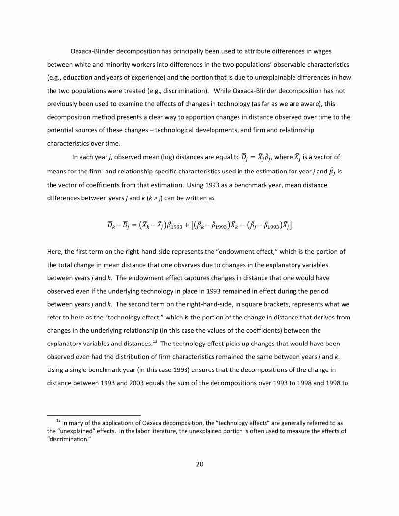
In each year j, observed mean (log) distances are equal to , where is a vector of
means for the firm‐ and relationship‐specific characteristics used in the estimation for year j and is
the vector of coefficients from that estimation. Using 1993 as a benchmark year, mean distance
differences between years j and k (k > j) can be written as
Here, the first term on the right‐hand‐side represents the “endowment effect,” which is the portion of
the total change in mean distance that one observes due to changes in the explanatory variables
between years j and k. The endowment effect captures changes in distance that one would have
observed even if the underlying technology in place in 1993 remained in effect during the period
between years j and k. The second term on the right‐hand‐side, in square brackets, represents what we
refer to here as the “technology effect,” which is the portion of the change in distance that derives from
changes in the underlying relationship (in this case the values of the coefficients) between the
explanatory variables and distances.12 The technology effect picks up changes that would have been
observed even had the distribution of firm characteristics remained the same between years j and k.
Using a single benchmark year (in this case 1993) ensures that the decompositions of the change in
distance between 1993 and 2003 equals the sum of the decompositions over 1993 to 1998 and 1998 to
12 In many of the applications of Oaxaca decomposition, the “technology effects” are generally referred to as
the “unexplained” effects. In the labor literature, the unexplained portion is often used to measure the effects of “discrimination.”

21
2003. Since we are interested in changes in distance since 1993, we believe that 1993 represents an
obvious choice of benchmark year.
Table 6 provides the detailed Oaxaca‐Blinder decomposition of the observed changes in distance
between 1993 and 2003. Distance changes are decomposed into the various firm‐ and relationship‐
specific groups used earlier.13 The results of the decomposition indicate that the total endowment
effect is significant and accounts for almost one‐quarter of the total change in mean distance over the
decade (table 6, column 1).14 Furthermore, the changes in firm‐ and relationship‐specific characteristics
– the endowment effect – had a positive effect on distance over both the 1993 to 1998 and 1998 to
2003 periods. The positive endowment effect was driven primarily by decreases in the share of
relationships that were with depository institutions or in the mix of products being supplied.
The remaining portion (about 75 percent) of the change in distance comprises the technological
effect, which represents the impact that technological or other changes may have had on distance
during the decade. Consistent with the results that we found for the pooled model, the total technology
effect suggests that distances increased during the first five years of the decade, again at a faster rate
than that found by Petersen and Rajan (2002), and declined thereafter. While the increase in the
technology effect between 1993 and 1998 and over the entire 10 year period were significant at the 1
percent level,15 the decline between 1998 and 2003 is not statistically significant.
If the technological changes were broad‐based, in that distances increased across the board for
all small businesses, then one would expect this to be captured by an increase in the constant term in
the estimations across the three survey years. This pattern is not observed. Over the entire decade, the
portion of the technological effect accounted for by the constant term is small, negative, and
insignificant. This suggests that whatever technological changes played out over the decade did not
affect all firms equally.
13 In the Oaxaca decomposition results, we report results for the endowment and technological effect for
groups of variables in the classes discussed earlier, such as creditworthiness and opacity. Most classes of variables considered contain several variables. While it is possible to decompose each variable’s effects on distance, grouping variables makes the discussion more tractable.
14 Column 1 of Table 5 indicates that log distances increased by .346, whereas the total endowment effect is associated with an increase in log distances of .082, accounting for approximately 25 percent of the total change (.082/.346).
15 For a detailed description of the procedure used to calculate the standard errors for the 1993‐2003 and 1998‐2003 Oaxaca‐Blinder decomposition estimates, please refer to Jann (2005) and Jann (2008). We use a bootstrapping procedure (with 10,000 draws) to estimate the standard errors for the 1998‐2003 decomposition estimates (with 1993 as the benchmark year).

22
The changes captured by the technological effect appear to be operating primarily through two
variable groups. Both groups have positive technology effects that were significant at the 5 percent
level over the decade, though the changes in each five‐year interval are generally not significant. The
group that contributed the most to changes in mean distance over time reflected firm management
characteristics. The technology effect for this group reflects the monotonic increases in the coefficients
on LOG_OWN1EXP across the three years of the SSBF (see table 4 above). As discussed in the previous
section, these coefficient changes imply that relationship distances involving firms with more
experienced ownership increased relative to relationships involving firms with less experienced
ownership over the decade.
The second group with a statistically significant technology effect was creditworthiness. Much
like firm management, the technology effect for this group is capturing monotonically increasing
coefficients on the two characteristics that comprise this group. Over time, the coefficients on CSPCT
and BADHIS became closer to zero. This reflects a larger increase in relationship distances at higher
quality firms (measured either by the credit score of the firm or the owner’s past credit history) relative
to lower quality firms.
These two groups were the largest contributors to the positive technology effect observed
between 1993 and 1998 (though only the effect of credit quality was significant at the 10 percent level
during this period). In the following five years, the effects of these groups remained positive, while the
overall technology effect became negative and insignificant. Nevertheless, contributions of both groups
during this second five year period were less than the effects observed in the earlier five year period,
suggesting that the rate of change for these two groups diminished in the latter portion of the decade.
The insignificant total technology effect in the latter five‐year period appears to derive from
offsetting effects across characteristic groups. Three characteristic groups – product type, financial
institution type, and length of relationship ‐‐ had significant technology effects in both five year periods.
However, their coefficients had opposite signs and similar magnitudes in the two five year periods.
Thus, these effects in the latter half of the decade appear to be something of a correction from what
was observed in the first half.
From the results of the Oaxaca‐Blinder decomposition, we are able to draw several conclusions.
Most of the increase in distance observed over the decade, and particularly during the first five‐year
period, played out differently across small firms primarily along characteristic dimensions related to
23
credit quality and firm ownership. The technology effect attributed to these groups fell substantially
during the latter portion of the decade, though they remained positive. The decline in mean
relationship distances observed between the 1998 and 2003 SSBFs appears to primarily reflect changes
that played out differently across product types that largely offset increases observed during the
previous five years.
While these results are useful in identifying the dimensions along which changes in distance
differed over time, it does not fully address questions about how distances actually changed over the
decade. In the next section, we use simulation to predict distances at different types of firms to
examine how distance changes occurred across firms.
STAGE 3: SIMULATIONS OF DISTANCE CHANGES
While the previous sections have established that the changes in distance did not occur uniformly across
small firms and that the dimensions of characteristic space along which the changes differed the most
related to credit quality and characteristics of the firm’s management, they have not addressed by how
much distances changed over the decade. In this section, we use simulation to demonstrate how the
change in distance varied across firms.
Our simulations focus on three hypothetical firms that are constructed to resemble firms in the
SSBF data. Firms in the data are subdivided into three groups based upon whether their age was three
years or less (“young firms”), greater than three years and less than ten (“middle age firms”), or ten or
more years (“mature firms”). Our analysis focuses on firm age because we believe this to be a better
measure of the opacity of the firm than would other measures, such as firm size.
Within each of these age bands, the median value for each firm‐specific characteristic, plus
length of relationship, was calculated.16 The exception is the industry dummy variables. The simulations
used values for these variables that are equal to the sample means for that dummy for all firms in that
age group. The values used for these characteristics in the simulations are shown in panel A of table 7.
The results show that younger firms tend to have shorter lengths of relationship with their creditors and
their primary owners tend to have fewer years of experience. They also tend to be smaller than older
firms and have lower credit scores. Finally, younger firms are more likely to be situated in local banking
16 For MSA*HERF, we used the product of the mean value of HERF and the median value of MSA, so that the
value for the interaction term was consistent with the values for these variables.

24
markets with fewer branches per square mile. Each of these patterns is monotonic across the three firm
age categories.
For each of these three hypothetical firms, distances were simulated for relationships involving
each of the five product types (e.g., lines of credit only, bundle). The remaining relationship‐specific
variables are all indicator variables. Each of these variables, DEPOSIT, CHECK, and COLLAT is assigned a
value of zero or one depending on the product type. If more than 50 percent of relationships involving
the provision of a specific product have the characteristic (use a depository institution, have a checking
account, or have collateral on the loan), then the variable is assigned a one. Otherwise, the indicator
variable for that characteristic is assigned a zero. Panel B of table 7 provides the share of relationships of
each product type that involved a depository institution, a checking account, or the pledging of
collateral. In the simulations, a share greater than 50 percent resulted in a value for that variable that
was equal to one. For example, relationships involving the provision of lines of credit only were
assumed to be with depository institutions (share=84.9%), include a checking account (share=66.2%),
and not involve the pledging of collateral (share=38.6%). Note that the values of these variables are
assumed to be constant across firm ages, so that differences in simulated distances across the three
firms solely reflect differences in firm‐ and relationship‐specific characteristics.
The simulations show that the increases in distance that we observed over the decade in the
unconditional means played out very differently across different types of firm and credit relationships.
Table 8 presents simulated distances for young, middle age, and mature firms for each of 5 product
types and for 3 survey years. Distances for relationships involving either a line of credit only or bundle
of loans were noticeably smaller than other credit relationship types and have not increased significantly
over the decade, holding constant the characteristics of the firm and the relationship.17 In stark
contrast, distances for relationships involving the provision of only asset‐backed loans increased
substantially over the decade for all three hypothetical firms with each increase significant at the 1
percent level. While the increase over the decade was substantial, a similar pattern of distances
increasing over the first five‐year period and contracting over the second period was observed for each
of the firm types, although the contraction from 1998‐2003 was statistically significant only for the
middle age and mature firms.
17 Significance tests were performed using the pooled regression model as a linear test of restrictions on the
coefficients.

25
The change in distances across these three hypothetical firms also suggests that increases in
distance over the decade were more substantial for the mature firm than the young or middle age firms.
In 1993, distances at the mature firm were lower for each of the five relationship types than they were
at the other two firms. In 2003, this pattern reversed itself and mature firms had slightly greater
distances in each of the relationship types than either of the younger firms. This suggests that the
technological changes that affected small business credit markets over this 10‐year period affected the
relationships of older firms more than younger firms.
The more rapid growth of distances involving older firms reflects, in part, the three firm
characteristics that were highlighted earlier as having experienced the largest change over the decade:
the firm’s credit score (CSPCT), the length of the primary owner’s experience (LOG_OWN1EXP), and the
number of bank branches per square mile in the market where the firm is located (DENSITY). Based
upon the medians used to determine the value of firm and relationship‐specific characteristics used in
the simulations, older firms have higher values for each of these three characteristics. Consequently,
relationship distances with older firms are increasing faster than distances at younger firms.
Conclusions
Recent technological changes have led some to question whether the traditional reliance of small
businesses on local suppliers of credit remains an important feature of small business credit markets.
Petersen and Rajan (2002), in particular, argue that productivity improvements at lending institutions
are steadily increasing distances between small businesses and their lenders. While their data only run
through 1993, they conjecture that the changes in distance that they find over the 1973 to 1993 period
accelerated after 1993.
In this paper, we use three years of the SSBF to assess this claim and to examine how mean
distances between small businesses and their suppliers of credit changed in the decade between 1993
and 2003. Our analysis leads us to draw three conclusions about how distances between small
businesses and their suppliers of credit changed over the decade.
The first conclusion that we draw from our analysis is that the distance increased during the first
five years of the decade at a faster rate than was reported by Petersen and Rajan (2002), but the
increases appear to have halted, or possibly even reversed, between 1998 and 2003. Distances in 1998
were approximately 40 percent higher than they had been in 1993, holding constant the characteristics

26
of the firm, financial institution, and product type involved in the relationship. This was followed by a 12
percent decline that left distances for the decade as a whole approximately 23 percent higher in 2003
than they had been in 1993.18
Our second conclusion, which is implied both by our rejection of the pooled regression model19
and the result of our Oaxaca‐Blinder decomposition, is that distance increases over the decade were
experienced differently across different types of firm, financial institution, and credit being supplied.
The results of our Oaxaca‐Blinder decomposition suggest that the increases in distance were primarily
related to the credit quality of the firm and characteristics of the firm’s ownership. In particular, while
high credit quality firms obtained credit from closer sources than lower quality firms in 1993, this
pattern had completely disappeared by the end of the decade with higher and lower credit quality firms
obtaining credit from suppliers at equal distances, other things equal. In addition, distances at firms
with more experienced owners increased relative to firms with less experienced owners.
Our third and final conclusion is that, based upon the simulations conducted in this paper, the
increases in distance over the decade were only experienced for some product types. In particular,
distances were found to have increased substantially over the decade for asset‐backed loans. Though
these relationships were conducted at somewhat shorter distances in 2003 than they had been in 1998,
the change over the decade as a whole remains substantial. On the other hand, distance increases for
relationships involving lines of credit or multiple credit product types (bundles) were effectively zero.
We also find that distance increases were much larger for older than for younger firms. This is
consistent with older firms having higher credit quality and more experienced management. While
older firms obtained credit from closer suppliers in 1993 than did younger firms, by 2003 this
relationship had inverted and older firms began to obtain credit at relatively greater distances than
younger firms.
Because this analysis relies upon a reduced form approach, we are unable to attribute the
changes highlighted in this study to demand or supply effects. Nevertheless, an examination of the
types of firm or credit relationship that experienced increase in distance can be informative in
understanding the likely causes of the increases in distance. In particular, a lot of attention in the
18 For details on how these changes were calculated, see Appendix A. 19 Recall that the pooled model assumes the coefficients do not vary across time. Using the fully‐interacted
pooled model, we reject the joint hypothesis that the coefficients on each variable are equal across survey years at the 1 percent level of confidence.

27
literature has been given to the role of technology in hardening information. Our analysis provides no
evidence that information opacity has decreased in its importance as a predictor of distance. In fact, for
younger and smaller firms, which are generally considered to be the most opaque, the growth of
distance lagged those of older and larger firms.
There is, therefore, little reason to believe, based upon these data that credit access to these
firms from more distant suppliers has increased over the decade. This suggests that, for antitrust policy
purposes, there is little evidence that the local geographic markets in which the smallest of these firms
obtain credit have increased significantly. This is particularly true for those credit products that were
supplied at the shortest distances at the start of the decade, lines of credit and bundles of credit
products. Instead, the increases in distance have primarily affected relationships that involve the
provision of asset‐backed loans, which at the beginning of the decade were already the most likely to be
provided by nonlocal suppliers. To the extent that antitrust policy is focused on preserving locally
competitive banking markets to ensure that these small firms that appear to be reliant on local suppliers
of credit are not subjected to uncompetitive loan terms, the evidence here argues against relaxing
antitrust policy towards banking mergers.
While there is little doubt that technology has had wide‐ranging effects on the banking industry,
the effects appear to be less revolutionary than some have conjectured (at least so far). However, it
appears clear that while distances between small firms and their suppliers of credit have increased, the
importance of geographic proximity persists in small business lending.
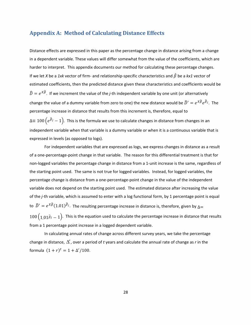
28
Appendix A: Method of Calculating Distance Effects
Distance effects are expressed in this paper as the percentage change in distance arising from a change
in a dependent variable. These values will differ somewhat from the value of the coefficients, which are
harder to interpret. This appendix documents our method for calculating these percentage changes.
If we let X be a 1xk vector of firm‐ and relationship‐specific characteristics and be a kx1 vector of
estimated coefficients, then the predicted distance given these characteristics and coefficients would be
. If we increment the value of the j‐th independent variable by one unit (or alternatively
change the value of a dummy variable from zero to one) the new distance would be . The
percentage increase in distance that results from this increment is, therefore, equal to
∆ 100 1 . This is the formula we use to calculate changes in distance from changes in an
independent variable when that variable is a dummy variable or when it is a continuous variable that is
expressed in levels (as opposed to logs).
For independent variables that are expressed as logs, we express changes in distance as a result
of a one‐percentage‐point change in that variable. The reason for this differential treatment is that for
non‐logged variables the percentage change in distance from a 1‐unit increase is the same, regardless of
the starting point used. The same is not true for logged variables. Instead, for logged variables, the
percentage change is distance from a one‐percentage‐point change in the value of the independent
variable does not depend on the starting point used. The estimated distance after increasing the value
of the j‐th variable, which is assumed to enter with a log functional form, by 1 percentage point is equal
to 1.01 . The resulting percentage increase in distance is, therefore, given by ∆
100 1.01 1 . This is the equation used to calculate the percentage increase in distance that results
from a 1 percentage point increase in a logged dependent variable.
In calculating annual rates of change across different survey years, we take the percentage
change in distance, , over a period of t years and calculate the annual rate of change as r in the
formula 1 1 ∆ /100.

29
Appendix B: Length of Relationship
A fundamental difference between the analysis undertaken here and that of Petersen & Rajan (2002)
involves the interpretation placed on the length of relationship between small firms and their suppliers
of credit. In the synthetic panel approach of Petersen & Rajan, the length of relationship reported in the
SSBF is used to calculate the calendar year in which the relationship began. For each calendar year
between 1973 and 1993, relationships reported to have begun in that year are used to estimate the
distances associated with that year’s lending activity. For example, observations in the synthetic panel
for 1985 were drawn from firm‐institution relationships that either were reported in the 1987 SSBF as
having been in existence for 2 years or were reported in the 1993 SSBF as having existed for 8 years.20
Using this approach Petersen & Rajan are able to examine how distances changed over a 20 year period,
using two cross sections of data taken 5 years apart.
With the benefit of hindsight, we believe that this methodology is subject to serious selection
biases that affect the mean (log) distances calculated for each calendar year under the synthetic panel
methodology. There are two potential sources of this bias. The first is firm survivorship bias in which
firms that borrow from more distant lenders may be less likely to survive over time. The second is
relationship survivorship bias, in which individual firms tend to maintain relationships with closer firms
over time, while discontinuing those with more distant suppliers. This bias would exist if relationships
with more distant suppliers are more likely single‐transaction relationships that last relatively few years
until a loan is paid off, as opposed to relationships that firms continue to renew over longer spans of
time. As a result of these survivorship biases, more distant relationships are less likely to be reported in
later surveys.
If present, these survivorship biases suggest that mean distances calculated for a given calendar
year using the synthetic panel methodology will decrease as the length of relationship increases. For
example, a survey of relationship distances conducted in year t might be expected to accurately reflect
the distances of relationships that began in year t. However, surveys taken in later years, if affected by
either firm‐ or relationship‐survivorship biases, would be expected to generate mean distances for year t
using the synthetic panel methodology that were lower than the means calculated from earlier surveys.
20 This is for those estimations in which PR used both the 1987 and 1993 SSBFs. In estimations that used only
the 1993 SSBF, the observations for 1985 came exclusively from those relationships that were reported as having been in existence for 8 years in the 1993 survey.

30
This is a consequence of longer‐distance relationships being less likely to survive until the time the later
survey is conducted. The implication of this bias would be that the synthetic panel methodology would
tend to understate mean distances in earlier years and overstate the change in distance over time.
The presence of these biases can be seen using a set of graphs similar to one that was used by
Petersen & Rajan (2002). The mean log relationship distance for all credit relationships using the
synthetic panel methodology is shown using the 1993 and 1998 SSBFs in figure A1 and using the 1998
and 2003 SSBFs in figure A2. Looking at the mean log distances for the first five years of overlap
between the 1998 and 2003 SSBFs (1994 to 1998) and between the 1993 and 1998 SSBFs (1989 to
1993), shows that in each case the mean log distances calculated using the earlier survey were higher
than those calculated using the later survey for four of the first five years. In each of these comparisons,
the lone exception is the calendar year in which the earlier survey was conducted where both the mean
log distance and the number of relationships upon which the mean was based are particularly low.21
This graph appears to show that in fact, the distances associated with each calendar year do seem to
decrease in the length of time between that year and the year in which the survey used to calculate the
distance was conducted.
To empirically test for the existence of this bias, we take the following approach. In the absence
of survivorship biases, the mean log distances calculated from each survey for any given calendar year
should be equal. We test this hypothesis using relationships that began during the years 1988 to 1998.
For each calendar year in which mean log distances can be computed using two or more SSBFs, we use a
Wald test of the hypothesis that the means are equal. The results of these tests are presented in table
A1.
The results presented in table A1 largely support the inferences drawn from figures A1 and A2.
Specifically, in four of the five first years of overlap between the 1998 and 2003 SSBFs, the difference in
mean log distances are positive and significant at the 5 percent level for 4 of the five years. Differences
in the first five years of comparison between the 1998 and 1993 SSBFs are positive and significant at the
5 percent level in 2 of the five years. There are no instances over this time period in which the means
calculated based on the earlier survey are lower than the means calculated using the later survey at
21 This pattern regarding mean log distances calculated for the calendar year in which the survey was conducted
is observed for all three survey years. Furthermore, these means are based upon fewer observations than recent years. In the 2003 SSBF, there were 10 relationships that began in 2003 compared to an average per year of 665 relationships for each of the next four years. The numbers for the 1998 and 1993 SSBFs show a similar pattern.

31
statistically significant levels. Furthermore, a joint test of the equality of means for the first five years of
overlap between all three SSBFs shows that the means are different at the 5 percent level of significance
for four of these five years.
The results of these tests suggest the existence of survivorship bias (or some other source of
bias) in which the mean log distances calculated for a calendar year decline as the length of time
between the calendar year and the year in which the survey is conducted increases. Consequently, the
synthetic panel approach, which identifies changes in distance from differences in the reported length of
relationships within each survey, should tend to overstate the change in distance over time as a result of
biases inherent in this methodology.

32
References
Amel, Dean F. and Kenneth P. Brevoort (2005). “The Perceived Size of Small Business Banking Markets,” Journal of Competition Law and Economics, 1(4): 771‐84.
Bauer, Thomas K., Markus Hahn and Mathias Sinning (2007). “Blinder‐Oaxaca Decomposition for Linear and Non‐linear Models,” speech delivered at the Fifth German Stata Users Group Meeting in Berlin, April 8.
Berger, Allen N., Adrian M. Cowan and W. Scott Frame (2009). “The Surprising Use of Credit Scoring in Small Business Lending by Community Banks and the Attendant Effects on Credit Availability and Risk,” Federal Reserve Bank of Atlanta Working Paper Series 2009‐9, March.
Berger, Allen N. and Gregory F. Udell (1998). “The Economics of Small Business Finance: The Roles of Private Equity and Debt Markets in the Financial Growth Cycle,” Journal of Banking and Finance, 22(6‐8): 613‐673.
Berger, Allen N. and Gregory F. Udell (2002). “Small Business Credit Availability and Relationship Lending: The Importance of Bank Organisational Structure,” The Economic Journal, 112(477): F32‐F53.
Black, Lamont K. (2009). “Information Asymmetries between Lenders and the Availability of Competitive Outside Offers,” Mimeo.
Blinder, Alan S. (1973). “Wage Discrimination: Reduced Form and Structural Estimates,” Journal of Human Resources, 8(4): 436‐455.
Board of Governors of the Federal Reserve System, Division of Research and Statistics (2008). Surveys of Small Business Finances, http://www.federalreserve.gov/pubs/oss/oss3/nssbftoc.htm (accessed October 14, 2008).
Boot, Arnoud W. A. (2000). “Relationship Banking: What Do We Know?” Journal of Financial Intermediation, 9(1): 7‐25.
Brevoort, Kenneth P. (2006). “An Empirical Examination of the Growth of Out‐of‐Market Commercial Lending: The Changing Competitive Landscape and the Role of Asymmetric Information,” Mimeo.
Brevoort, Kenneth P. and Timothy H. Hannan (2006). “Commercial Lending and Distance: Evidence from Community Reinvestment Act Data,” Journal of Money, Credit, and Banking, 38(8): 1991‐2012.
Brevoort, Kenneth P. and John D. Wolken (2009). “Does Distance Matter in Banking?” in Pietro
Alessandrini, Michele Fratianni, and Alberto Zazarro, eds., The Changing Geography of Banking and
Finance. New York: Springer publishers.

33
Cowan, Charles D. and Adrian M. Cowan (2006). “A Survey Based Assessment of Financial Institution Use of Credit Scoring for Small Business Lending,” SBA Office of Advocacy Report, November.
Critchfield, Tim, Tyler Davis, Lee Davison, Heather Gratton, George Hane and Katherine Samolyk
(2004). “The Future of Banking in America: Community Banks: Their Recent Past, Current
Performance, and Future Prospects,” FDIC Banking Review, vol. 16 (3), pp. 1‐56.
DeYoung, Robert, W. Scott Frame, Dennis Glennon, Daniel P. McMillen, and Peter J. Nigro (2008). “Commercial Lending Distance and Historically Underserved Areas,” Journal of Economics and Business, 60(1‐2): 149‐164.
DeYoung, Robert, W. Scott Frame, Dennis Glennon, and Peter Nigro (2007b). “What’s Driving Small Borrower‐Lender Distance?” Working paper.
DeYoung, Robert, Dennis Glennon, and Peter Nigro (2008). “Borrower‐Lender Distance, Credit Scoring, and Loan Performance: Evidence from Informationally‐Opaque Small Business Borrowers,” Journal of Financial Intermediation, 17(1): 113‐143.
DeYoung, Robert, William C. Hunter and Gregory F. Udell (2004). “The Past, Present, and Probable
Future for Community Banks,” Journal of Financial Services Research, Vol. 25, pp. 85‐113.
Frame, W. Scott, Aruna Srinivasan, and Lynn Woosley (2001). “The Effect of Credit Scoring on Small‐Business Lending,” Journal of Money, Credit and Banking, 33(3): 813‐825.
Frame, W. Scott, Michael Padhi, and Lynn Woosley (2004). “Credit Scoring and the Availability of Small Business Credit in Low‐ and Moderate‐Income Areas,” Financial Review, 39(1): 35‐54.
Hannan, Timothy H. (2003). “Changes in Non‐Local Lending to Small Business,” Journal of Financial Services Research, 24(1): 31‐46.
Horrace, William C. and Ronald L. Oaxaca (2001). “Inter‐industry Wage Differentials and the Gender Wage Gap: An Identification Problem,” Industrial and Labor Relations Review, 54(3): 611‐618.
Hyytinen, Ari and Mika Pajarinen (2007), “Opacity of Young Businesses: Evidence from Rating Disagreements,” Journal of Banking and Finance, 32(7): 1234‐1241.
Jann, Ben (2005). “Standard Errors for the Blinder‐Oaxaca Decomposition,” paper presented at the Third German Stata Users Group Meeting, held in Berlin, April 8.
________, (2008). “The Blinder‐Oaxaca decomposition for linear regression models.” The Stata Journal 8(4): 473‐479.
Kwast, Myron L., Martha Starr‐McCluer, and John D. Wolken (1997). “Market Definition and the Analysis of Antitrust in Banking,” The Antitrust Bulletin, 42 (4): 973‐95.
Laderman, Elizabeth S. (2008). “The Quantity and Character of Out‐of‐Market Small Business Lending,” Economic Review, pp. 31‐38.
34
Norden, Lars, and Martin Weber (2008). “Credit Line Usage, Checking Account Activity, and Default Risk of Bank Borrowers,” Mimeo.
Oaxaca, Ronald L. (1973). “Male‐female Wage Differentials in Urban Labor Markets,” International Economic Review, 14(3): 693‐709.
Oaxaca, Ronald L. and Michael R. Ransom (1994). “On Discrimination and the Decomposition of Wage Differentials,” Journal of Econometrics, 61(1): 5‐21.
________, (1999). “Identification in Detailed Wage Decompositions,” The Review of Economics and Statistics, 81(1): 154‐157.
Petersen, Mitchell A. and Raghuram G. Rajan (1994). “The Benefits of Lending Relationships: Evidence from Small Business Data,” Journal of Finance, 49(1): 3‐37.
________, (1995). “The Effect of Credit Market Competition on Lending Relationships,” Quarterly Journal of Economics, 110(2): 407‐442.
________, (2002). “Does Distance Still Matter? The Information Revolution in Small Business Lending,” Journal of Finance, 57(6): 2533‐2570.
Scott, Jonathan A. (2003), “Credit, Banks and Small Businesses – The New Century: A Research Perspective,” Mimeo.
Scott, Jonathan A. and William C. Dunkelberg (2003). “Bank Mergers and Small Firm Financing,” Journal of Money, Credit, and Banking, 35(6): 999‐1017.
United States Government Accountability Office (2007). “Additional Measures Needed to Assess 7(a)
Loan Program’s Performance,” GAO Report GAO‐07‐769.
Wolken, John D. and Douglas Rohde (2002). “Changes in the Location of Small Businesses' Financial
Services Suppliers Between 1993 and 1998, ” Board of Governors of the Federal Reserve System
Memo.

Table 1: Distance Measures in the Survey of Small Business Finances, 1993, 1998, and 2003
1993 1998 2003 1993 1998 2003 1993 1998 2003 1993 1998 2003 1993 1998 2003
All Relationships 110.6 242.9 180.6 2.6 3.0 2.9 27.9 34.0 34.6 8 8 11 4,969 3,637 5,276
Relationships by Institution Type
Depositories 42.3 84.5 74.6 1.8 1.9 2.0 12.4 13.3 17.1 4 3 4 3,198 2,318 3,218
Commercial Banks 40.5 84.0 75.4 1.8 1.9 2.0 12.3 13.1 16.5 3 3 4 2,910 2,103 2,804
Thrifts 57.9 102.8 80.3 2.0 2.1 2.1 13.0 14.1 19.7 5 4 5 190 128 263
Nondepositories 249.8 552.7 357.4 4.0 5.1 4.4 59.5 74.6 63.6 47 252 52 1,771 1,319 2,058
Finance Companies 214.7 470.3 361.9 3.9 4.9 4.4 58.7 72.8 63.1 41 221 51 929 802 1,597
Leasing Companies 299.5 753.6 305.8 4.2 5.6 4.3 60.7 83.8 67.1 57 461 52 741 419 309
Mortgage Companies 283.5 667.2 406.9 4.4 5.1 4.6 59.7 72.6 68.6 145 272 53 19 48 63
Relationships by Product Type
Lines of Credit Only 58.1 134.2 90.4 2.0 2.0 1.9 13.7 15.9 14.5 4 3 3 1,257 918 1,503
Mortgages Only 92.0 204.0 143.5 2.3 2.5 2.9 20.5 22.8 36.0 6 5 15 289 366 450
Asset‐backed Only 162.9 385.2 286.4 3.2 4.1 3.9 41.7 56.3 54.6 20 75 38 2,406 1,665 2,409
Other Loans Only 78.7 73.9 199.8 2.1 1.7 3.0 18.8 10.1 36.5 4 2 20 277 92 106
Bundled Loans 26.2 48.9 38.1 1.5 1.7 1.7 7.9 9.5 9.1 2 3 4 740 596 808
NOTE: Mean and median distances are expressed in miles.
Mean Distance Mean Log Distance
Percent Nonlocal
(>30 miles) Median Distance Number of Observations

Table 2: P‐Values of Univariate Tests of Means
1993 =
1998
1998 =
2003
1993 =
2003
1993 =
1998
1998 =
2003
1993 =
2003
1993 =
1998
1998 =
2003
1993 =
2003
All Relationships 0.000 0.000 0.000 0.000 0.356 0.000 0.000 0.686 0.000
Relationships by Institution Type
Depositories 0.000 0.401 0.001 0.421 0.032 0.001 0.487 0.004 0.000
Commercial Banks 0.000 0.509 0.001 0.396 0.116 0.009 0.528 0.018 0.002
Thrifts 0.300 0.587 0.502 0.820 0.743 0.513 0.811 0.246 0.139
Nondepositories 0.000 0.000 0.000 0.000 0.000 0.001 0.000 0.000 0.073
Finance Companies 0.000 0.002 0.000 0.000 0.000 0.000 0.000 0.001 0.128
Leasing Companies 0.000 0.000 0.912 0.000 0.000 0.617 0.000 0.001 0.203
Mortgage Companies 0.024 0.077 0.370 0.334 0.344 0.821 0.427 0.705 0.586
Relationships by Product Type
Lines of Credit Only 0.000 0.040 0.037 0.829 0.474 0.551 0.280 0.458 0.681
Mortgages Only 0.010 0.139 0.144 0.387 0.028 0.002 0.584 0.002 0.001
Asset‐backed Only 0.000 0.000 0.000 0.000 0.022 0.000 0.000 0.420 0.000
Other Loans Only 0.902 0.067 0.071 0.061 0.000 0.004 0.048 0.000 0.015
Bundled Loans 0.071 0.545 0.413 0.071 0.769 0.112 0.452 0.884 0.544
Distance Log Distance Percent Nonlocal (>30 miles)

Table 3: Summary Statistics: Sample Means(1) (2) (3) (4)
1993 Only 1998 Only 2003 Only Pooled
Dependent Variable
Log of Distance (LOG_DIST) 2.561 2.965 2.907 2.824
Distance (DIST) 110.543 242.904 181.089 178.911
Firm‐Specific Characteristics
Creditworthiness
Credit Score (CSPCT) 49.094 51.91 53.287 51.675
Bad History (BADHIS) 0.237 0.191 0.2 0.208
Opacity
Firm Age (LOG_FAGE) 2.441 2.438 2.503 2.466
Assets (LOG_ASSETS) 12.016 11.787 11.855 11.881
Corporation (CORP) 0.606 0.567 0.596 0.590
Has Records (RECORDS) 0.475 0.799 0.596 0.621
Management
Owner Experience (LOG_OWN1EXP) 2.825 2.824 2.919 2.864
Managed by Owner (MGR) 0.839 0.895 0.933 0.895
Local Market Characteristics
Market Concentration (HERF) 0.161 0.173 0.167 0.167
MSA 0.798 0.782 0.784 0.788
MSA*HERF 0.105 0.113 0.110 0.110
Branch Density (DENSITY) 0.11 0.116 0.124 0.118
Non‐Market Offices (NONMKT) 0.111 0.109 0.102 0.106
National Sales Area (NATIONAL) 0.114 0.136 0.149 0.135
Industry
Transportation 0.039 0.050 0.056 0.049
Construction 0.144 0.146 0.157 0.150
Manufacturing 0.106 0.095 0.081 0.092
Wholesale Trade 0.099 0.085 0.074 0.085
Retail Trade 0.218 0.176 0.174 0.187
Insurance and Real Estate 0.071 0.07 0.073 0.071
Personal Services 0.165 0.213 0.217 0.201
Professional Services 0.158 0.165 0.169 0.165
Relationship‐Specific Characteristics
Financial Institution Type
Depository (DEPOSIT) 0.67 0.662 0.625 0.649
Product Characteristics
Lines of Credit Only (LOC) 0.244 0.27 0.313 0.280
Mortgages Only (MORT) 0.065 0.116 0.097 0.093
Other Loans Only (OTHLN) 0.062 0.026 0.02 0.034
Asset‐backed Only (ASSET) 0.506 0.453 0.455 0.469
Bundled Loans (BUNDLE) 0.124 0.135 0.116 0.124
Collateral (COLLAT) 0.825 0.763 0.747 0.774
Checking Account (CHECK) 0.432 0.428 0.393 0.415
Length of Relationship
Lenth of Relationship (LOG_REL) 1.758 1.693 1.766 1.742
Observations 4,964 3,635 5,152 13,751
NOTE: Variable names are shown besides characteristic names when variables have been defined in
the text.

MEMO:
Firm Specific Characteristics
CreditworthinessCredit Score (CSPCT) ‐0.003 *** ‐0.0003 0.0004 ‐0.001 0.050
(0.001) (0.001) (0.001) (0.001)
Bad History (BADHIS) 0.084 0.081 ‐0.007 0.06 0.712(0.074) (0.098) (0.092) (0.052)
Opacity
Firm Age (LOG_FAGE) ‐0.055 ‐0.024 ‐0.037 ‐0.033 0.936(0.056) (0.067) (0.060) (0.037)
Assets (LOG_ASSETS) 0.038 ** 0.023 0.011 0.021 * 0.569(0.018) (0.021) (0.018) (0.012)
Corporation (CORP) ‐0.050 0.071 ‐0.018 ‐0.004 0.521(0.069) (0.082) (0.078) (0.046)
Has Records (RECORDS) 0.101 * 0.033 0.146 ** 0.122 *** 0.623(0.060) (0.092) (0.071) (0.043)
Management
Owner Experience (LOG_OWN1EXP) ‐0.074 0.033 0.130 * 0.053 0.086(0.059) (0.078) (0.072) (0.042)
Manged by Owner (MGR) ‐0.062 0.138 ‐0.102 ‐0.013 0.324(0.078) (0.125) (0.136) (0.064)
Local Market Characteristics
Market Concentration (HERF) 0.794 ** 0.661 1.013 ** 0.802 *** 0.879(0.386) (0.518) (0.483) (0.286)
Urban Area (MSA) 0.12 0.303 0.477 *** 0.323 *** 0.309(0.153) (0.204) (0.177) (0.108)
MSA*HERF ‐0.212 ‐1.698 * ‐1.699 ** ‐1.353 *** 0.288(0.740) (0.921) (0.752) (0.475)
Branch Density (DENSITY) ‐0.2 0.09 ‐0.853 *** ‐0.384 ** 0.102(0.270) (0.361) (0.302) (0.184)
Nonmarket Offices (NONMKT) 0.214 ** 0.108 0.234 ** 0.204 *** 0.669(0.091) (0.109) (0.104) (0.061)
National Sales Area (NATIONAL) 0.131 0.087 0.364 *** 0.210 *** 0.139(0.101) (0.119) (0.102) (0.064)
Industry
Construction ‐0.325 ** ‐0.271 ‐0.080 ‐0.205 * 0.624(0.161) (0.199) (0.200) (0.119)
Manufacturing ‐0.021 ‐0.242 ‐0.465 ** ‐0.241 ** 0.225(0.167) (0.209) (0.197) (0.120)
Wholesale Trade ‐0.241 ‐0.102 ‐0.374 * ‐0.257 ** 0.654(0.173) (0.209) (0.209) (0.122)
Retail Trade ‐0.183 ‐0.282 ‐0.400 ** ‐0.298 *** 0.680(0.159) (0.191) (0.189) (0.114)
Insurance and Real Estate ‐0.346 * ‐0.482 ** ‐0.068 ‐0.236 * 0.428(0.177) (0.225) (0.234) (0.136)
Personal Services ‐0.358 ** ‐0.161 ‐0.292 ‐0.244 ** 0.735(0.162) (0.192) (0.193) (0.116)
Professional Services ‐0.221 ‐0.456 ** ‐0.515 *** ‐0.408 *** 0.468(0.170) (0.193) (0.194) (0.117)
P-Values of H0: 1993=1998=2003
Table 4: Regression Results for Individual Years and Pooled Model(4)
Pooled1993 Only
(1)
1998 Only
(2)
2003 Only
(3)

Table 4: Regression Results for Individual Years and Pooled Model (continued)
MEMO:
P-Values of H0: 1993=1998=2003
(4)
Pooled1993 Only
(1)
1998 Only
(2)
2003 Only
(3)
Relationship Specific Characteristics
Financial Institution Type
Depository Institution (DEPOSIT) ‐1.277 *** ‐1.982 *** ‐1.137 *** ‐1.433 *** 0.000(0.099) (0.128) (0.116) (0.069)
Product Characteristics
Lines of Credit Only (LOC) 0.061 ‐0.275 ** ‐0.193 ‐0.120 * 0.055(0.088) (0.126) (0.120) (0.067)
Mortgages Only (MORT) ‐0.105 ‐0.442 *** ‐0.08 ‐0.206 ** 0.119(0.145) (0.139) (0.133) (0.083)
Other Loans Only (OTHLN) ‐0.200 ‐0.931 *** 0.148 ‐0.300 *** 0.002(0.128) (0.215) (0.266) (0.111)
Bundled Loans (BUNDLE) ‐0.151 * ‐0.168 ‐0.118 ‐0.118 * 0.954(0.088) (0.119) (0.117) (0.064)
Collateral (COLLAT) ‐0.053 ‐0.183 * 0.056 ‐0.029 0.211(0.081) (0.096) (0.096) (0.055)
Checking Account (CHECK) ‐1.264 *** ‐1.485 *** ‐1.609 *** ‐1.489 *** 0.029(0.085) (0.116) (0.102) (0.060)
Length of Relationship
Length of Relationship (LOG_REL) ‐0.173 *** ‐0.297 *** ‐0.155 *** ‐0.201 *** 0.103(0.049) (0.054) (0.045) (0.030)
Constants
D1998 0.345 ***
(0.051)
D2003 0.215 ***
(0.048)
Constant 4.405 *** 5.305 *** 4.12 *** 4.292 ***
(0.329) (0.399) (0.387) (0.228)
Observations 4,964 3,635 5,152 13,751 13,751
R‐squared 0.38 0.48 0.40 0.41
F‐Statistic 67.09 89.27 68.63 187.35 4.041
F-Statistic p-Value 0.0000 0.0000 0.0000 0.0000 0.0000
Variable names are shown beside characterisitc names when variables have been defined in the text.
* significant at 10%; ** significant at 5%; *** significant at 1%.
Note: In each estimation the dependent variable is the log of distance (LOG_DIST ). Standard errors in parentheses.
P‐values in Memo column are for a Wald test of whether the three coefficients for each variable in the fully‐interacted model are
equal. The resulting test statistic is distributed as F(2,13735). 1This is the Wald statistic for the joint test that the coefficients on each variable (yearly intercept) was constant across the three
time periods. It is distributed as F(67,13670).

Table 5: P‐Values of Joint Significance Tests of Characteristic Groups(1) (2) (3) (4)
1993 Only 1998 Only 2003 Only Pooled
Firm Specific Characteristics
Creditworthiness (2) 0.001 0.663 0.941 0.203
Opacity (4) 0.076 0.560 0.292 0.011
Management (2) 0.328 0.503 0.131 0.438
Local Market Characteristics (6) 0.020 0.524 0.000 0.000
Industry (7) 0.055 0.096 0.005 0.021
Relationship Specific Characteristics
Financial Institution Type (1) 0.000 0.000 0.000 0.000
Product Characteristics (6) 0.000 0.000 0.000 0.000
Length of Relationship (1) 0.001 0.000 0.001 0.000
Numbers in parentheses represent the number of variables in each characteristic group.
NOTE: P‐values are calculated for a Wald statistic of the hypothesis that the coefficients of a
characteristic group are jointly zero. For example, the creditworthiness group,
the hypothesis tested is that the coefficients on CSPCT and BADHIS are both zero. These statistics are
based on the coefficients reported in table 4.

Difference 0.346 *** 0.404 *** ‐0.058 (0.045) (0.047) (0.050)
Endowment Effect
Firm‐Specific
Creditworthiness ‐0.017 *** ‐0.013 *** ‐0.004 **(0.004) (0.004) (0.002)
Opacity 0.003 0.026 ‐0.023 *(0.009) (0.021) (0.013)
Management ‐0.013 ‐0.003 ‐0.009 (0.009) (0.004) (0.006)
Industry ‐0.011 * ‐0.007 ‐0.004 *(0.006) (0.005) (0.002)
Local Market Characteristics 0.003 0.008 ‐0.005 *(0.008) (0.008) (0.003)
Relationship‐Specific
Financial Institution Type 0.058 *** 0.010 *** 0.047 ***(0.004) (0.001) (0.004)
Product Type 0.065 *** 0.010 0.055 ***(0.011) (0.010) (0.005)
Length of Relationship ‐0.001 *** 0.011 *** ‐0.013 ***(0.000) (0.003) (0.004)
Total Endowment Effect 0.086 *** 0.042 * 0.044 ***(0.021) (0.025) (0.016)
Technology Effect
Firm‐Specific
Creditworthiness 0.219 *** 0.155 * 0.064 (0.083) (0.086) (0.094)
Opacity ‐0.274 ‐0.120 ‐0.154 (0.358) (0.381) (0.395)
Management 0.579 ** 0.380 0.199 (0.282) (0.283) (0.320)
Industry 0.002 0.012 ‐0.010 (0.025) (0.025) (0.185)
Local Market Characteristics ‐0.197 ‐0.048 ‐0.149 (0.140) (0.155) (0.206)
Relationship‐Specific
Financial Institution Type 0.018 ‐0.114 *** 0.132 ***(0.019) (0.026) (0.027)
Product Type ‐0.033 0.115 ** ‐0.147 **(0.066) (0.057) (0.073)
Length of Relationship 0.033 ‐0.210 * 0.242 **(0.118) (0.124) (0.122)
Constant
Constant ‐0.087 0.192 ‐0.279 (0.421) (0.427) (0.454)
Total Technology Effect 0.260 *** 0.362 *** ‐0.102 (0.051) (0.054) (0.086)
NOTE: Standard errors are in parantheses.
* significant at 10%; ** significant at 5%; *** significant at 1%.
Table 6: Oaxaca Decomposition of Changes in Distance by Characteristic Group
1993 to 2003 1993 to 1998 1998 to 2003
(1) (2) (3)

Table 7: Characteristic Values Used in Distance Simulations
(1) (2) (3)
Creditworthiness
Credit Score (CSPCT) 44 46 64
Bad History (BADHIS) 0 0 0
Opacity
Firm Age (LOG_FAGE) 1.099 1.946 3.045
Assets (LOG_ASSETS) 11.432 11.572 12.165
Corporation (CORP) 1 1 1
Has Records (RECORDS) 0 1 1
Management
Owner Experience (LOG_OWN1EXP) 2.398 2.398 3.258
Managed by Owner (MGR) 1 1 1
Local Market Characteristics
Market Concentration (HERF)
Urban Area (MSA) 1 1 1
MSA*HERF 0.129 0.151 0.136
Branch Density (DENSITY) 0.074 0.081 0.092
Non‐Market Offices (NONMKT) 0 0 0
National Sales Area (NATIONAL) 0 0 0
Industry
Construction 0.096 0.146 0.173
Manufacturing 0.088 0.099 0.080
Wholesale Trade 0.111 0.067 0.085
Retail Trade 0.221 0.187 0.157
Insurance and Real Estate 0.078 0.049 0.075
Personal Services 0.199 0.239 0.192
Professional Services 0.136 0.155 0.179
Transportation 0.071 0.058 0.059
Length of Relationship
Length of Relationship (LOG_REL) 1.099 1.609 1.946
(1) (2) (3)
Share at Depository (DEPOSIT)
Share with Checking (CHECK)
Share with Collateral (COLLAT)
Product Characteristics
Lines of Credit Only (LOC) 84.9 66.2 38.6
Mortgages Only (MORT) 64.1 28.4 88.6
Other Loans Only (OTHLN) 27.7 16.6 29.7
Asset‐backed Loans Only (ASSET) 34.0 12.1 100.0
Bundled Loans (BUNDLE) 93.4 83.7 72.6
Panel A: Firm Characteristics
Panel B: Relationship Characteristics
NOTE: Variable names are shown besides characteristic names when variables have been defined in the text.
Young Firm
Middle Age
Firm Mature Firm

1993 1998 2003
Lines of Credit Only 5.1 5.3 3.7 0.2 ‐1.6 ** ‐1.4 *
Mortgages Only 14.6 16.5 22.1 1.9 5.6 * 7.5
Other Loans Only 50.0 88.2 81.7 38.2 * ‐6.5 31.6
Asset‐backed Loans Only 58.0 186.3 74.5 128.4 *** ‐111.9 16.5 ***
Bundled Loans 3.9 4.9 4.2 1.0 ‐0.7 0.3
Lines of Credit Only 5.0 4.5 3.8 ‐0.4 ‐0.7 ** ‐1.2
Mortgages Only 14.1 14.0 22.5 ‐0.1 8.4 ** 8.4 **
Other Loans Only 48.4 75.0 83.1 26.6 8.1 * 34.7
Asset‐backed Loans Only 56.1 158.5 75.8 102.4 *** ‐82.7 ** 19.7 ***
Bundled Loans 3.8 4.2 4.3 0.4 0.1 0.5
Lines of Credit Only 3.9 4.1 4.0 0.2 ‐0.2 0.0
Mortgages Only 11.2 12.9 23.5 1.7 10.6 *** 12.3 ***
Other Loans Only 38.3 68.9 86.9 30.5 ** 18.0 *** 48.6
Asset‐backed Loans Only 44.4 145.5 79.2 101.1 *** ‐66.3 *** 34.8 ***
Bundled Loans 3.0 3.8 4.5 0.8 * 0.7 *** 1.5 NOTE: * significant at 10%; ** significant at 5%; *** significant at 1%.
1993 to
1998
1998 to
2003
1993 to
2003
Young
Firm
Middle
Age
Firm
Mature
Firm
Simulated Means
(in miles)
Change In Distance
(in miles)
Table 8: Simulated Distances by Firm Age Group and Product Type: 1993, 1998,
and 2003

1998 0.4841997 0.0291996 0.0001995 0.0001994 0.0001993 0.404 0.633 0.6781992 0.003 0.497 0.0001991 0.686 0.013 0.0171990 0.996 0.016 0.0261989 0.330 0.352 0.0301988 0.600 0.020 0.034
Table A1: P‐Values for Mean Tests of Synthetic Panel, 1988‐1998
Test Conducted
Calendar Year 2003 = 1998 1998 = 1993 2003 = 1998 = 1993

35
Figure A1: Mean Log Distances from Synthetic Panels, 1993 and 1998 SSBFs
Figure A2: Mean Log Distances from Synthetic Panels, 1998 and 2003 SSBFs


