
Discrete Prices and the Incidence and Efficiency of Excise Taxes
Christopher T. Conlon∗ Nirupama L. Rao†
April 20, 2019‡
AbstractThis paper uses detailed UPC-level data from Nielsen to examine the relationship between excisetaxes, retail prices, and consumer welfare in the market for distilled spirits. Empirically, we doc-ument the presence of a nominal rigidity in retail prices that arises because firms largely chooseprices that end in ninety-nine cents and change prices in whole-dollar increments. Theoretically,we show that this rigidity can rationalize both highly incomplete and excessive pass-through esti-mates without restrictions on the underlying demand curve. A correctly specified model, such asan (ordered) logit, takes this discreteness into account when predicting the effects of alternative taxchanges. We show that explicitly accounting for discrete pricing has a substantial impact both onestimates of tax incidence and the excess burden cost of tax revenue. Quantitatively, we documentsubstantial non-monotonicities in both of these quantities, expanding the potential scope of whatpolicymakers should consider when raising excise taxes.
Keywords: Excise Tax, Incidence, Market Power, Price Adjustment, Nominal Rigidities.
JEL Classification Numbers: H21, H22, H71.
∗[email protected], New York University Stern School of Business. 44 W 4th St New York, NY.†[email protected], Ross School of Business, University of Michigan. 701 Tappan Avenue, Ann Arbor, MI 48109‡The authors would like to acknowledge valuable input and advice from: Wojciech Kopczuk, Bernard Salanie,
Jon Vogel, Kate Ho, Juan Carlos Surez Serrato, Sebastien Bradley and seminar participants at Columbia University,Wharton BEPP, Duke University, NYU Stern, the National Tax Association 2014 Annual Conference, IIOC 2015,the 2016 NASM of the Econometric Society and the Ross School of Business at the University of Michigan. Anyremaining errors are our own. Researchers own analyses calculated (or derived) based in part on data from TheNielsen Company (US), LLC and marketing databases provided through the Nielsen Datasets at the Kilts Centerfor Marketing Data Center at The University of Chicago Booth School of Business The conclusions drawn from theNielsen data are those of the researcher(s) and do not reflect the views of Nielsen. Nielsen is not responsible for, hadno role in, and was not involved in analyzing and preparing the results reported herein
1

1. Introduction
Pass-through describes how changes in costs relate to changes in prices and conveys the extent
to which cost shocks are borne by consumers or firms. As a measure of incidence, pass-through
determines the welfare implications of cost shocks such as exchange rate fluctuations, commodity
price spikes and taxes.
In this paper we examine the pass-through of recent increases in excise taxes on distilled spirits
in Connecticut, Illinois and Louisiana using high-quality scanner data from Nielsen. We first
provide descriptive evidence of the price responses to tax increases in the three states and to match
the prior literature estimate pass-through rates using linear regression. We find evidence of over-
pass-through, particularly for smaller containers which saw smaller tax increases, though estimates
vary over different horizons. Examining price changes we next document the pricing behaviors
that underlie these responses. We find that the majority of price changes are made in large, fixed
increments – most frequently in whole-dollar amounts. Retailers do not react to taxes by smoothly
increasing prices but instead either leave a price unchanged or increase prices sharply most often by
$1 or $2 to one of a handful of favored price points. In light of the pricing behaviors we document
and the rigidities they imply, we then estimate discrete choice models to better approximate the
pricing patterns we see in the data. Finally, we use these estimates to predict how prices will change
in response to tax increases of different magnitudes and simulate the resulting incidence and social
cost of tax revenue. These simulations show that the over-pass-through arising from these price
point rigidities strongly shifts the tax burden on to consumers and leads to substantial dead-weight
loss.
We take a different, though complementary, approach from the literature on optimization fric-
tions. Instead of exploiting discontinuities in the tax schedule as a source of exogenous variation
to recover a frictionless, long-run structural elasticity, we explicitly model the endogenous but dis-
continuous pricing strategies of firms in response to taxes. Our goal is not to recover the structural
relationship between prices and taxes that would arise in a frictionless world, but rather to model
how pricing rigidities would respond to alternative tax policies, and to understand the welfare
implications in such a world.
In spirit our analysis is most related to Nakamura and Zerom (2010) and Goldberg and Heller-
stein (2013). Both of those papers allow for nominal rigidities and examine the transmission of
cost shocks into prices using scanner data, though neither paper studies the impact of taxes. Both
papers find limited pass-through in the coffee and beer industries, respectively. In contrast with
these findings, we find that pass-through of excise taxes on distilled spirits is nearly immediate
(within a month) and is often over-shifted (in excess of 100%).1 One possible discrepancy is that
1These pass-through results are not directly comparable. Because we measure the impact of a per-unit excise taxand are worried about $1 price changes, we measure pass-through of taxes in dollars to retail prices in dollars ordollar for dollar pass-through. The aforementioned studies measure pass-through by examining percentage changesin retail prices as caused by percentage changes in input prices or exchange rates. In order to reconcile these types
2

exchange rate or commodity price fluctuations are likely to be perceived as transitory, while excise
tax changes are likely to be perceived as permanent, leading to a higher share of price increases.
Price changes at the time of tax changes may also be less costly for retailers because consumer
awareness of the tax change may lower ‘customer antagonization’ costs (Anderson and Simester,
2010).
Consistent with our descriptive evidence, previous studies using a small number of brands have
found that alcohol taxes are over-shifted (pass-through ∂P∂τ > 1). Cook (1981) found that the
median ratio of annual price change to tax change for leading brands in the 39 state-years that had
tax changes between 1960 and 1975 was roughly 1.2. Young and Bielinska-Kwapisz (2002) followed
the prices of seven specific alcoholic beverage products and estimated pass-through rates ranging
from 1.6 to 2.1. When Alaska more than doubled its alcohol taxes in 2002, Kenkel (2005) reported
that the associated pass-through was between 1.40 to 4.09 for all alcoholic beverages, and between
1.47 to 2.1 for distilled spirits. All three studies report substantial product-level heterogeneity in
the degree of pass-through.
The over-shifting of taxes is not limited to taxes on distilled spirits, nor are all excise taxes
over-shifted. For sales taxes Poterba (1996) found that retail prices of clothing and personal care
items rise by approximately the tax amount while Besley and Rosen (1999) could not reject full
pass-through for some goods, but found evidence of over-shifting for more than half of the goods
they studied. In fuels, where price increments are very small (often one cent) relative to tax
changes, studies have found that gasoline and diesel taxes are fully passed through to consumers
though prices may not fully adjust when supply is inelastic or inventories were high (Marion and
Muehlegger, 2011) and that gas tax holidays are pass-though quickly but only partially to consumers
(Doyle Jr. and Samphantharak, 2008). Harding et al. (2012) found that cigarette taxes were less
than fully passed through to consumers, while DeCicca et al. (2013) could not reject full pass-
through of cigarette taxes on average, but found that consumers willing to shop faced significantly
less pass-through. In another retail setting where price points may be important, Besanko et al.
(2005) found that 14% of wholesale price-promotions were passed on at more than 100% into retail
prices.
Estimated pass-through rates exceeding unity, like those we estimate, have been theoretically
justified by the presence of imperfect competition among suppliers and curvature restrictions on
demand. Most of those results employ a single-product homogenous good framework. Katz and
Rosen (1985), Seade (1985), and Stern (1987) all rely on Cournot competition with conjectural vari-
ations and curvature restrictions. Besley (1989) and Delipalla and Keen (1992) employ a Cournot
model with free entry and exit, and rely taxes pushing out competing brands to generate overshift-
ing. This literature is summarized in Fullerton and Metcalf (2002). Because Cournot competition
may not be a realistic assumption for many taxed goods including distilled spirits, Anderson et al.
of estimates we would need a measure of the original marginal cost of spirits products.
3

(2001) develop similar results under differentiated Bertrand competition. The common thread is
that demand must be sufficiently (log)-convex in order to generate overshifting. However, as An-
derson et al. (2001) point out, as demand becomes too convex, the marginal revenue curves may
no longer be downward sloping. Thus theoretical attempts to justify over-shifting may lead to un-
realistic restrictions on demand curves. Fabinger and Weyl (2012) categorize the pass-through rate
and marginal revenue properties of several well-known demand systems, and show that satisfying
both properties is difficult but possible. In a recent and notable departure from this theoretical
literature, Hamilton (2009) finds that excise taxes can lead to overshifting when demand is suf-
ficiently concave rather than convex but requires strategic complementarities between prices and
variety and that higher taxes lead to reduced variety of product offerings.
As we observe over-shifting, but not brand exit in response to the tax; these long-run explana-
tions of over-shifting are not well matched to our data. Instead, we show that a nominal rigidity
like price points can generate over-shifting or under-shifting of taxes without restrictions on the
curvature of the underlying demand curve.
The focus on price points is not unique to our setting. A literature which documents the presence
of price points as a source of nominal rigidities in macroeconomics includes: Kashyap (1995), Knotek
(2010b) and Levy et al. (2011).2 Other work has focused on the role of “convenient prices” – round
prices that coincide with monetary denominations (Knotek, 2008), (Knotek, 2010a). Ours is first
examination of the implications of price points for tax incidence and efficiency. The phenomenon
of price points extends beyond distilled spirits. Tabulations of the Nielsen data demonstrate that
prices are concentrated at a handful of price points in many product market. Approximately 40.1%
of all prices are set at at one of the four most common price points for each product category. At
the product category level, in more than 49% of the 1,113 product categories of the Nielsen data,
at least half of all prices in each category are set at one of the four most common price points per
category. The discrete pricing patterns that we observe are not unique to spirits; retailers price
discretely in many product markets.
2A deeper question is: “Why do we observe ninety-nine cent prices?” One potential explanation is that consumersexhibit “left digit bias” and do not fully process information. This idea is explored in Lacetera et al. (2012). Anotherexplanation might be that firms consider only a smaller number of discrete price points for cost or informationprocessing reasons. For further discussion of just-below prices please see Schindler (2011). While interesting, these“why” explanations are beyond the scope of our paper. Other work shows that left-digit bias can benefit firms. Basu(2006) demonstrates that in oligopolistic markets with fully rational consumers who nonetheless exhibit left-digitbias firms benefit when consumers ignore the last digits of a price, even under Bertrand competition. In recent workShlain (2018) uses Nielsen data to show that consumers respond to a one cent increase from a 99-ending price as ifit were a 15 to 25 cent difference and firms respond to this bias with high shares of 99-ending prices and missinglow-ending prices, though they do not fully exploit the profit potential of left-digit bias. Krishna and Slemrod (2003)suggest that tax authorities themselves may exploit left-digit bias in setting tax rates like for example the 39.6% toptax rate that prevailed from 1993 until 2001.
4
2. Alcohol Taxation and Industry Background
Distilled spirits are one of the most heavily taxed commodities in the United States, with the
combined state and federal tax burden comprising as much as 30-40% of the retail price. In
2010, total tax revenues on distilled spirits contributed $15.5 billion, for an industry in which
production, distribution and retailing amount to roughly $120 billion in revenue. Since 1991, the
federal government has taxed distilled spirits at $13.50 per proof-gallon, or $4.99 for a 1.75L bottle
of 80-proof vodka.3 The statutory incidence of federal excise taxes falls on the producers of distilled
spirits or is due upon import into the United States. Our paper focuses on state excise taxes, which
are remitted by wholesalers and usually levied by volume rather than ethanol content. Posted prices
at both retail and wholesale levels include both state and federal excise taxes. In some states, there
is an additional sales tax tacked on to the retail price that applies only to alcoholic beverages, while
in others alcoholic beverages are exempt from the general sales tax.
As a consequence of the 21st Amendment, states are free to levy their own taxes on spirits, as
well as regulate the market structure in other ways. There are 18 control states, where the state
has a monopoly on either the wholesale distribution or retailing of alcohol beverages (or both).4
Connecticut, Illinois, Louisiana, and 29 other states are license states. License states follow a three-
tier system where vertically separated firms engage in the manufacture, wholesale distribution, and
retailing of alcohol beverages. Almost all license states have restrictions that prevent distillers from
owning wholesale distributors, or prevent wholesale distributors from owning bars or liquor stores.
In the three states we study, wholesalers and retailers are fully distinct.5
All of these taxes are of course levied in part to address the negative health and public safety
externalities of alcohol. However, governments also tax alcohol for the explicit purpose of raising
revenue.6 Few states had changed their alcohol taxes over the prior decade, but following the onset
of the Great Recession, eight states passed legislation affecting alcohol taxes. We report those tax
changes in Table 1. We focus on three recent tax changes.
Prior to July 1, 2011, the state of Connecticut levied a tax on the volume of distilled spirits
3Taxes are stated in customary units of gallons, though products are sold internationally in standardized metricunits of 750mL, 1L, and 1.75L bottles. A proof-gallon is 50% alcohol by volume (100 Proof) at 60 degrees Fahrenheit.
4The monopoly applies to all alcohol beverages in some states, and in others to distilled spirits but not wine orbeer. Control states can adjust markups or taxes to raise revenue. A few control states, such as Maine and Vermont,nominally control the distribution and sales of spirits but contract with private firms which set prices. Control stateshave been the subject of recent empirical work examining the entry patterns of state-run alcohol monopolies Seimand Waldfogel (2013) and the effects of uniform markup rules Miravete et al. (2018).
5States have other restrictions on the number of retail licenses available, or the number of licenses a single chainretailer can own. States also differ on which types of alcoholic beverages, if any, can be sold in supermarkets andconvenience stores.
6For example, in 2015 Governor Sam Brownback of Kansas proposed raising alcohol and tobacco taxes to help closethe state’s $648 million budget shortfall. For more details see http://www.kansas.com/news/politics-government/
article6952787.html. In 2016, Governor Jon Bel Edwards of Louisiana proposed a similar tax increase which wouldraise $27 million, as part of reducing a $900 million deficit, see http://www.nola.com/politics/index.ssf/2016/
03/house_passes_new_alcohol_tax_h.html.
5

(independent of proof) of $4.50 per gallon, which worked out to $2.08 per 1.75L bottle.7 After
July 1, 2011, the tax increased to $5.40 per gallon, or $2.50 on a 1.75L bottle, for an increase of
$0.24 per liter. In September 2009, Illinois increased its excise tax from $4.50 per gallon to $8.55
per gallon, or an additional $1.07 per liter. Louisiana raised taxes in April 2016 only slightly from
$2.50 to $3.03 per gallon or $0.14 per liter.
It should be noted that Connecticut and Louisiana also raised their sales taxes from 6% to
6.35% and from 4% to 5%, respectively, at the same time that they increased their alcohol excise
taxes. Our empirical analysis examines the impact of the specific tax increase on sales-tax-exclusive
retail prices. As sales taxes are levied at the time of retail sale and added onto the posted price,
any pass-through of the sales tax increases would lead to lower retail prices. Thus the pass-through
rates we report for Connecticut and Louisiana potentially under-estimate the true excise tax pass-
through rates. We also estimate pass-through rates using sales-tax-inclusive prices; our estimates
are mechanically larger but statistically indistinguishable from the results presented here.
Our empirical exercise focuses more specifically on the July 2011 tax increase in Connecticut.
We do this for a few reasons that exploit some institutional details around the Connecticut tax
increase. First, the Connecticut state regulator forbids wholesalers or retailers from engaging in
temporary sales, coupons, price promotions, or giveaways; retail “sales” must be registered with
the Department of Consumer Protection in advance, and are limited to a small number of clearance
items. The retail price data reveal few if any temporary sales; ignoring the first week of the month
(which may cover two months), there is virtually no within product-store-month price variation in
Connecticut. Because weekly prices in the Nielsen data are calculated as revenue divided by unit
sales, this means we can say with some confidence that the prices observed in our data accurately
describe the prices observed by consumers in Connecticut. It also means that we do not need
to distinguish between general price changes and short-term markdowns.8 A second important
provision of the Connecticut tax increase ensured that the tax was uniform on all units sold after
the tax increase. Retailers (and wholesalers) were subjected to a floor tax on unsold inventory as
of July 1, 2011. By making the tax impact immediate for all units, this means that we can be
certain all units sold at retail after July 1 were subject to the higher tax rate.9
While we also use data from the Illinois and Louisiana tax increases, the institutional details
in those states are a bit different. Both states allow temporary sales, loyalty card discounts, and
coupons on distilled spirits. This means we should be cautious about interpreting weekly variation
in average prices paid (particularly small changes) as actual price changes by retailers. Likewise,
7Many states levy lower tax on lower-proof ready-to-drink products, or lower-proof schnapps and liqueurs.8How one handles temporary sales is one of the principal challenges in the empirical macroeconomics literature on
estimating menu costs. See Levy et al. (1997), Slade (1998), Kehoe and Midrigan (2007), Nakamura and Steinsson(2008), Eichenbaum et al. (2011), Eichenbaum et al. (2014).
9The floor tax meant that any product not in the hands of consumers would be subjected to the new tax raterather than the old tax rate, and prevented retailers from evading the tax by placing large orders in advance of the taxincrease. It did not, however, prevent consumers from stockpiling alcoholic beverages in advance of the tax increase,though we find no evidence of an anticipatory price effect.
6

we cannot find evidence either way for whether a floor tax was employed in Illinois and Louisiana,
so there may have been identical products on the retailer’s shelf taxed under different regimes, and
thus the effect of tax changes on retail prices may have been less immediate.
3. Data
Our primary data source is the Kilts Nielsen Scanner dataset. The Nielsen data are a substantial
improvement over previous price data in the alcohol tax literature; much of the prior literature
relies on the ACCRA Cost of Living Index data, which survey a small number of products and
stores in each state. Nielsen provides weekly scanner data, which track revenues and unit sales at
the UPC (universal product code) level for a (non-random) sample of stores in all 50 states, though
in practice we only have sufficient data on distilled spirits from 34 states.10 These weekly data
are available from 2006-2016, and include data from both stand-alone liquor stores as well as from
supermarkets and convenience stores. Participation in the Nielsen dataset is voluntary, and not all
stores participate. The data contain many more supermarkets than stand-alone liquor stores, and
many stores in the sample are affiliated with a larger chain. This leads to better coverage for states
where spirits are sold in supermarkets. In Connecticut, we observe 34 (mostly larger) stand-alone
liquor stores. Because spirits are also available in supermarkets in Illinois and Louisiana, we observe
884 and 310 stores respectively.11 While the raw data are organized weekly, for our analyses we
aggregate our data to the store-product-month level or the store-product-quarter level. For prices,
we use the price from the last full week entirely within that month or quarter.12
For the state of Connecticut only, we are able to use a special dataset we constructed of the
(tax inclusive) prices that wholesalers charged retailers from August 2007 to August 2013.For more
details on this dataset and how it is constructed, please consult Appendix B. As one might expect,
and as our results will indicate, wholesale prices serve as an important state variable for retailer
pricing decisions. For some of our welfare calculations, we utilize estimated product-level marginal
costs from a structural model of supply and demand from Conlon and Rao (2015).
We summarize our main (monthly) dataset in Table 2. For each state and product size (750mL,
1L, 1.75L) we report the number of store-product-month observations, the total sales, and the
average price paid (total revenue divided by total sales). We exclude 1L bottles from Illinois and
Louisiana because we have fewer than 8,000 such observations and they represent a very small
fraction of sales; we keep them for Connecticut where they represent around 8% of the market.
Additionally, we report the size of the tax increase for each state and product size which ranges from
10We lack sufficient data from 16 states, many of which are control states (in italics): Alabama, Alaska, Hawaii,Idaho, Kansas, Montana, New Hampshire, New Jersey, North Carolina, Oklahoma, Oregon, Pennsylvania, RhodeIsland, Tennessee, Utah, Vermont, Virginia.
11We lack sufficient data to study the 2013 excise tax increase (and sales tax decrease) in Rhode Island or the2009 excise tax increase in New Jersey, in part because those states only allow spirits to be sold in stand alone liquorstores.
12For additional details on aggregation, please consult Appendix B.
7

$0.105 per bottle for 750mL bottles in Louisiana to $1.87 per bottle for 1.75L bottles in Illinois.
We also consider a weighted version of the same sample where we weight products by their annual
sales in the same store for the calendar year prior to tax change. This means we weight products
in CT based on 2010 sales, IL based on 2008 sales, and LA based on 2015 sales.13 We use these
weights because price changes are more important for more popular products.14 The weighted
sample has substantially lower prices because mass-market products are cheaper and more popular
than high-end niche products. One downside is that products with no sales during these years are
effectively dropped from the sample. We also have very different numbers of observations from
different states. To address this, we normalize our weights so that each state receives equal weight
in our overall sample.15 We also observe that prices are broadly similar in Louisiana and Illinois,
but substantially higher in Connecticut.16
4. Descriptive Evidence and Linear Pass-Through Estimates
4.1. Monthly Price Changes
We first summarize observed price changes in each state by month and year, highlighting the
month when taxes increased. Table 3 reports unweighted average monthly retail price changes
for Connecticut, Illinois, and Louisiana for the years surrounding their recent tax changes and
demonstrates three facts. First, there is a regular, seasonal component to price changes with prices
increasing in some months like January and July and decreasing in others like February. Second, in
both Connecticut and Illinois retail prices immediately and sharply increased in the month of the
tax hikes with mean retail price increases of $0.316 in Connecticut and $0.651 in Illinois, which are
substantially larger than price increases in those months in other years, and larger than the average
tax increase. In Louisiana where taxes were increased by $0.15 on average, prices only increased
modestly by $0.186 in the month of the tax change. We find evidence of delayed responses with
an even larger response of $0.787 in Illinois in the month following the tax change and a smaller
than typical May price decline in Louisiana. Finally, we don’t find much evidence (except perhaps
Connecticut in June for $0.133) of prices increasing in anticipation of the tax change, even though
the laws were passed months prior.
These average price changes are driven in part by more frequent price changes. Figure 3
plots the sales-weighted fraction of retail products experiencing price changes and price increases
each month in each state. There is a substantial spike in the frequency of price adjustment (and
especially price increases) commensurate with the tax increases in Connecticut (July 2011) and
13Our weighting is meant to mimic the Laspeyres price index. We don’t weight using contemporaneous sales(Paasche), because we expect that demand curves slope downwards and we don’t want to systematically underweightproducts with larger price increases.
14In total we observe 6,785 products many of which have extremely low sales. We consider restricting the sampleto the top 1000 or top 500 products and it has almost no effect on any of the estimates we report.
15Later we also balance our weights so that each state and product size combination receives equal weight.16We examine the laws which facilitate collusive wholesale pricing in Conlon and Rao (2015).
8

Illinois (September 2009). The spike in Connecticut is more explicit in part because the state bans
temporary sales resulting in lower baseline adjustment frequencies. In Louisiana, however, the
April 2016 tax change is associated with an increase but not a large spike in the frequency of price
changes or increases. Instead price changes and increases spike three months later in July 2016,
a month generally associated with price increases in Louisiana. In total these patterns suggest we
should analyze the price impact of a potential tax change over a longer window of time (such as
three months) rather than simply examining the immediate impact.
4.2. Linear Regression Estimates of Pass-Through
Following the large literature on pass-through, we measure the pass-through rate using a linear
regression of price changes ∆pjst on tax changes ∆τjst where j denotes product, s denotes store, t
denotes month and the ∆ operator denotes the difference taken over time within a store and product.
We follow the convention for excise tax pass-through and measure both changes in dollars. Thus
the pass-through rate, ρ(·), denotes the expected price increase (in dollars) for a $1 tax increase.
We estimate the pass-through parameter with fixed effects for UPC, as well as month-of-year
and year.
∆pjst = ρjst(X,∆τ) ·∆τjt + β∆xjst + γj + γt + εjst (1)
We have written the pass-through rate ρjt(X,∆τ) as a general function that might depend on
(j, t) as well as other covariates X, or the size of the tax change itself, ∆τ . Most of the literature
assumes that for “small” tax changes, pass-through is approximately constant. For example, Besley
and Rosen (1999) and Harding et al. (2012) assume a single pass-through rate ρjt(X,∆τ) = ρ, or
product specific pass-through ρjt(X,∆τ) = ρj respectively.
We estimate the regression (1) pooling observations from all three states, but interacting ρjt(·)with each state and package size (750mL, 1L, 1.75L) which we report in Table 4. This is a semi-
parametric regression in the sense that for each observed value of ∆τjt we estimate a distinct
pass-through rate. We report the 7 estimates (we drop 1L bottles in IL and LA) for one-month,
three-month, and six-month horizons to address the concern that retail prices may not respond
immediately.17. Finally, we provide two sets of estimates in separate panels. The left panel reports
the pass-through rates estimated from the full sample, while the right reports the pass-through
estimates conditional on a price changes. Under the hypothesis that all tax changes are smoothly
passed on to price changes, we would expect these two sets of parameter estimates to be identical.
There are some important patterns which emerge from Table 4. The first is that pass-through
is nearly immediate in Connecticut where the one-month and three month estimates are nearly
17For example, Table 3 indicates retail prices may vary with a predictable schedule not aligned with tax changes.While Section 2 discusses that absent an explicit floor tax Louisiana and Illinois retailers may hold inventories notsubjected to higher tax rates for several months.
9

identical; while pass-through is slower in Illinois and Louisiana. This may be because the timing
of the tax change in Connecticut was commensurate with the month when retailers traditionally
adjusted prices, or it may be because of the floor tax. Later, at the six month window pass-through
estimates often (though not always) attenuate. In part this may be because retailers adjust prices
for other reasons in addition to the tax change, this is particularly true in Louisiana (see Table 3
and Figure 3) where large price changes are more frequent.18
When we focus on three-month pass-through rates, we see that five of the seven state-size
combinations have estimated pass-through rates which are statistically > 1 and are closer to 2 than
to 1. Consistent with prior work on taxation of distilled spirits, this suggests that tax changes are
overshifted, or that a $1.00 tax change is met with a more than $1.00 price change. In general, the
pattern also suggests that larger tax changes are met with smaller pass-through rates. To see this
relationship more explicitly we plot the seven pass-through estimates for three-month price changes
in the left panel of Figure 4. When we pool the data for all states and estimate the pass-through
rate as a weighted linear function of the tax change we find that ρ(∆τ) = 1.76− 0.51 ·∆τ , which
we also plot on Figure 4.19 This implies that the pass-through rate of an infinitesimal tax increase
would be 176% and for a $1.00 tax increase would be 125%.
If we compare the left and right panes of Table 4, we see pass-through estimates conditional
on any price changes are substantially larger than overall estimates of pass-through. This suggests
that tax changes were not smoothly passed on into price changes but instead that a large number of
products experience no price change in response to the tax, while other products experience a larger
price change than the average pass-through rate suggests. These conditional estimates along with
the pass-through rates implied by a $1 and $2 price change are plotted in the right panel of Figure
4. If the observed tax changes resulted in price changes of exactly $1, estimated pass-through rates
would lie on the first dotted line; if all prices changed by $2, the estimates would lie on the second
dotted line. What we observe is that both LA estimates and the CT estimate for 750mL products
lie very close to the $1 line while the IL estimate for 1.75L products lies close to the $2 line and IL
estimate for 750mL products suggests a mix of $1 and $2 price changes. The other CT estimates
for 1L and 1.75L products at three-months are somewhat lower than implied by a strict $1 price
change rule though the one-month conditional estimates (3.29 and 2.00) would line up well.
This suggests the correct way to think about the pass-through rate may not be as a constant ap-
plied to any size tax change, but rather that the pass-through rate we measure may be a mechanical
relationship between large price change increments and the size of the tax.
18Also recall that we include state-product specific fixed effects (trends) in (1) which are generally positive.19We consider higher order functions of ∆τ . Both the quadratic and cubit function are indistinguishable from the
linear function.
10

5. Price Points and Pass-Through
The analyses in the previous section suggest that three-months is a more appropriate interval to
analyze retail responses to tax changes. Therefore, we document several facts by examining the
frequency of price endings and categorizing price changes using quarterly data. We focus on the
idea that retailers utilize a small number of price points and that the bulk of price changes are in
increments of $1.00.
Later, we write down a dynamic model of price adjustment with discrete price points. We show
how to estimate the policy function from the dynamic pricing model using an ordered logit. Using
the ordered logit estimates, we re-calculate pass-through, welfare, and deadweight loss and compare
them to estimates from the linear (constant pass-through) model.
5.1. Observed Price Points
We begin by documenting the relatively small number of price points used by retailers in the
Nielsen scanner dataset. From 5,479,724 observations of quarterly prices we construct a transition
probability matrix using just the cents portion of price. A product which sold for $10.99 for two
quarters in a row would be recorded as a price that previously ended in $0.99 cents and still is
priced at a price ending in $0.99, as would a product which increased in price to $11.99. Table
5 presents transition frequencies for each state detailing how the cents portions of prices compare
from quarter to quarter.
As these matrices show, retailers set prices at and change prices to a small set of price points
that account for a large share of overall prices. The most common price ending is 99 cents and it
accounts for 78% of prices in Louisiana, 80% in Illinois, and 91% in Connecticut. Not all retailers
use 99 cents as their default price ending, one chain in Illinois uses 97 cents and two chains in
Louisiana use 49 cents instead. We aggregate price endings outside of the ten most common into
the other category, which ranges from 1.35% in CT to 5.93% in IL.20
We expect that Table 5 understates the actual concentration of price points, even though the
two most common price endings account for at least 85% of prices in every state. In addition to
alternative conventions among a few chains, some retailers appear to use other price points (such
as 19 cents or 95 cents) as internal tracking for sale or clearance items. Further, as we discuss in
Section 3 Nielsen reported prices, particularly in Illinois and Louisiana where sales and discounts
are more common, may not coincide with any transacted prices when prices change midweek.21 We
try to address these issues, and describe the steps we take in Appendix C.2, but they remain.
The key consequence of this small number of price points is that when firms adjust prices
20If we normalize the rows of each matrix to sum to one, we can treat these as Markov Transition ProbabilityMatrices. In the long-run (ergodic) distribution we find that the share of prices outside of the ten most commonprice points would be 1.22%, 5.77% and 3.46%, meaning that the long-run stationary distribution of prices and themarginal distribution of prices are highly similar.
21This also helps explain why 99 to 99 transitions are more common in Connecticut than in other states. As wenote in Section 2, Connecticut also does not allow coupons, loyalty cards, and makes temporary sales very difficult.
11
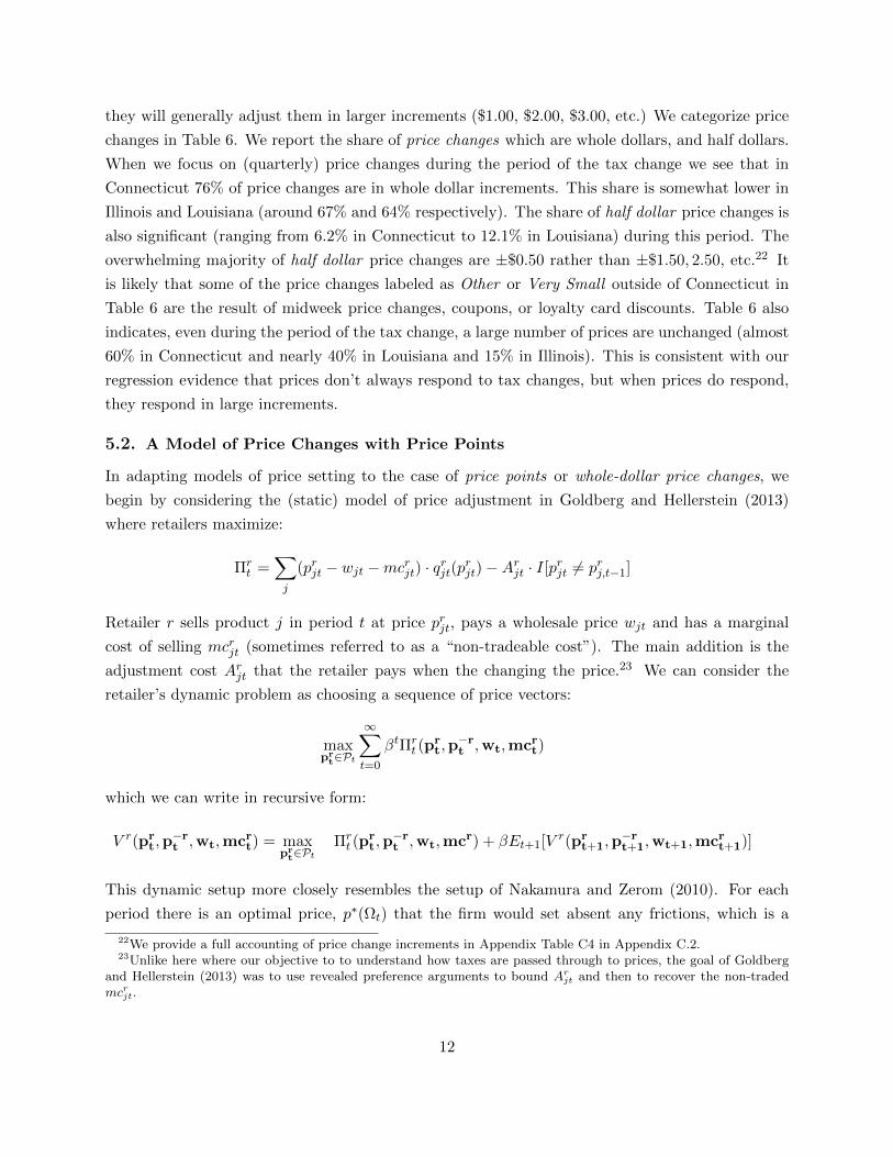
they will generally adjust them in larger increments ($1.00, $2.00, $3.00, etc.) We categorize price
changes in Table 6. We report the share of price changes which are whole dollars, and half dollars.
When we focus on (quarterly) price changes during the period of the tax change we see that in
Connecticut 76% of price changes are in whole dollar increments. This share is somewhat lower in
Illinois and Louisiana (around 67% and 64% respectively). The share of half dollar price changes is
also significant (ranging from 6.2% in Connecticut to 12.1% in Louisiana) during this period. The
overwhelming majority of half dollar price changes are ±$0.50 rather than ±$1.50, 2.50, etc.22 It
is likely that some of the price changes labeled as Other or Very Small outside of Connecticut in
Table 6 are the result of midweek price changes, coupons, or loyalty card discounts. Table 6 also
indicates, even during the period of the tax change, a large number of prices are unchanged (almost
60% in Connecticut and nearly 40% in Louisiana and 15% in Illinois). This is consistent with our
regression evidence that prices don’t always respond to tax changes, but when prices do respond,
they respond in large increments.
5.2. A Model of Price Changes with Price Points
In adapting models of price setting to the case of price points or whole-dollar price changes, we
begin by considering the (static) model of price adjustment in Goldberg and Hellerstein (2013)
where retailers maximize:
Πrt =
∑j
(prjt − wjt −mcrjt) · qrjt(prjt)−Arjt · I[prjt 6= prj,t−1]
Retailer r sells product j in period t at price prjt, pays a wholesale price wjt and has a marginal
cost of selling mcrjt (sometimes referred to as a “non-tradeable cost”). The main addition is the
adjustment cost Arjt that the retailer pays when the changing the price.23 We can consider the
retailer’s dynamic problem as choosing a sequence of price vectors:
maxprt∈Pt
∞∑t=0
βtΠrt (p
rt,p−rt ,wt,mcrt)
which we can write in recursive form:
V r(prt,p−rt ,wt,mcrt) = max
prt∈Pt
Πrt (p
rt,p−rt ,wt,mcr) + βEt+1[V r(pr
t+1,p−rt+1,wt+1,mcrt+1)]
This dynamic setup more closely resembles the setup of Nakamura and Zerom (2010). For each
period there is an optimal price, p∗(Ωt) that the firm would set absent any frictions, which is a
22We provide a full accounting of price change increments in Appendix Table C4 in Appendix C.2.23Unlike here where our objective to to understand how taxes are passed through to prices, the goal of Goldberg
and Hellerstein (2013) was to use revealed preference arguments to bound Arjt and then to recover the non-tradedmcrjt.
12
function of the state variables Ωt = p−rt ,wt,mcrt, Xt. As the marginal costs or demand shocks
accumulate over time, the gap between prt and p∗ grows until the firm pays the cost Arjt and updates
its price. Here rather than choosing a continuous p∗ our firms chose among a discrete grid of points
pt+1 ∈ Pt ≡ pt + ∆pt where ∆pt ∈ . . . ,−2,−1, 0, 1, 2, . . ..24 When prices are chosen among a
discrete set, the first-order conditions need not hold exactly, leading to a large number of potential
solutions and no good algorithm to find them.25
We focus on a specific set of counterfactuals which depend only on the policy functions in the
language of Bajari et al. (2007).26 This avoids ever solving for an equilibrium of the pricing problem,
but it means we cannot separately identify the menu costs A. Because we have a small number of
tax changes, it also means we are limited in our ability to consider changes in the state variables
Ωt or their transition f(Ωt+1|Ωt). We consider a policy function of the form Pr(∆pjt|∆τjt,Ωt) and
ask: “How would prices respond if we held everything else fixed, but varied the size of the tax
change?” This means if we estimate policy functions using three-month changes, we are explicitly
considering how other tax changes would affect three month price changes. We are not modeling
what might happen in the longer run if higher taxes cause retailers to price differently years later.
Likewise, we should be cautious about interpretation of long-run behavior of agents outside the
model (such as if manufacturers reduce annual price increases in response to the tax change). If
there are menu costs, agents take them into account when making decisions, but we cannot separate
them in welfare calculations.
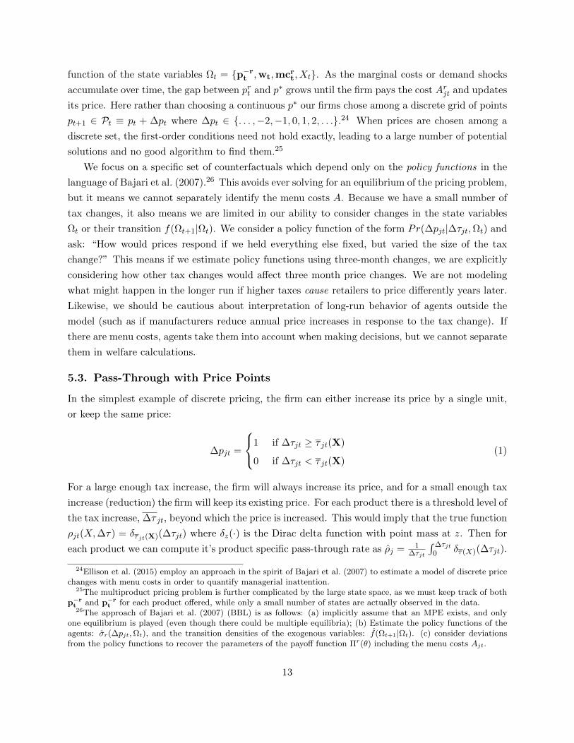
5.3. Pass-Through with Price Points
In the simplest example of discrete pricing, the firm can either increase its price by a single unit,
or keep the same price:
∆pjt =
1 if ∆τjt ≥ τ jt(X)
0 if ∆τjt < τ jt(X)(1)
For a large enough tax increase, the firm will always increase its price, and for a small enough tax
increase (reduction) the firm will keep its existing price. For each product there is a threshold level of
the tax increase, ∆τ jt, beyond which the price is increased. This would imply that the true function
ρjt(X,∆τ) = δτ jt(X)(∆τjt) where δz(·) is the Dirac delta function with point mass at z. Then for
each product we can compute it’s product specific pass-through rate as ρj = 1∆τjt
∫ ∆τjt0 δτ(X)(∆τjt).
24Ellison et al. (2015) employ an approach in the spirit of Bajari et al. (2007) to estimate a model of discrete pricechanges with menu costs in order to quantify managerial inattention.
25The multiproduct pricing problem is further complicated by the large state space, as we must keep track of bothp−rt and p−r
t for each product offered, while only a small number of states are actually observed in the data.26The approach of Bajari et al. (2007) (BBL) is as follows: (a) implicitly assume that an MPE exists, and only
one equilibrium is played (even though there could be multiple equilibria); (b) Estimate the policy functions of theagents: σr(∆pjt,Ωt), and the transition densities of the exogenous variables: f(Ωt+1|Ωt). (c) consider deviationsfrom the policy functions to recover the parameters of the payoff function Πr(θ) including the menu costs Ajt.
13

This pass-through rate takes on only two values for each j: 1∆τjt
or 0. Ignoring other covariates,
the OLS estimates of the pass-through rate from (1) are a weighted average of product level pass-
through ρ =∑
jtwjtρj .
This demonstrates how it is possible to generate either incomplete pass-through or over-shifting.
For example, if ∆τ = 0.25 and products are equally weighted, wj = 1J , then ρ, our OLS estimate of
pass-through, would be a weighted average of ρj = 4 and ρj = 0. As long as more than 14 products
increase their price in response to the tax, it is possible to estimate ρ ≥ 1 without imposing
special conditions on the demand function, while if fewer products increase their price we will find
incomplete pass-through (ρ < 1).
Figure 1 illustrates the price response with a binary logit. Because the x-axis represents the tax
change, and the y-axis represents the price change, the OLS estimate of the pass-through rate is the
slope of a ray intersecting the sinusoidal curve, ρ = ∆p∆τ . The complete pass-through ρ = 1 line is in
yellow for reference. For a small tax increase (red line), it might be that very few products change
prices so that the estimated pass-through rate is small. For a very large tax increase (blue line) the
price of most products may increase, but this might be smaller (or larger) than the denominator,
∆τ . For some intermediate value of the tax increase, it might be that most products increase their
prices, but that ∆τ is not so large, leading to a higher estimate of the pass-through rate. If we
plot the slope of each ray to the same S-shaped curve, we would find that the implied pass-through
rate is U-shaped: rising during the steep part of the S-curve and falling over the flat parts. If we
expanded the support of potential tax changes (and the potential outcomes of our price change
model), price changes would follow a series of S-shaped curves, and pass-through would follow a
series of U-shaped curves.
In general we do not expect the econometrician to observe ∆τ jt(X) directly, and instead it must
be estimated. If we allow for some econometric error in ∆τ jt(X) that is IID and type I extreme
value: then this suggests that the correct estimator for ρjt(X,∆τ) is the predicted probability from
a logit (divided by the tax increase): Pr(∆p=1|X,∆τ)∆τ . Our empirical specification extends this model
to an ordered logit and allow for larger price increases (or price decreases).
With enough variation in the support of ∆τ , the linear model from (1) can trace out any re-
lationship between tax changes and price changes ρjt(X,∆τ), including a nonlinear relationship
with discrete price changes such as an (ordered) logit. By exploiting our knowledge that price
changes are in whole-dollar increments, we can impose some nonlinearity on the relationship be-
tween price changes and tax changes ex ante, and obtain more reasonable estimates with limited
support for ∆τ . This is especially important when we want to forecast for tax changes not ob-
served in the data. If we estimate a large pass-through rate for an observed tax increase, the linear
model would apply that pass-through rate to a larger increase; the nonlinear model might interpret
a large pass-through rate as the top of the U-shaped curve and anticipate less pass-through for
larger tax changes. This is crucial for measuring the welfare cost of these taxes, because declining
14

pass-through rates mean not only that taxes fall more on firms than on consumers, but also that
they generate less deadweight loss per dollar of government revenue.
5.4. Estimating Pass-Through with Price Points
To address whole-dollar price changes, we estimate ordered logit models of the form:
∆psjt = k if Y ∗sjt ∈ [αk, αk+1]
Y ∗sjt = f(∆τjt, θ1) + g(wjt, psjt, θ2) + h(psjt, p−s,jt, θ3) + βXsjt + γt + εsjt (2)
where we restrict ∆pfjt ∈ −$1.00, 0,+$1.00,+$2.00,+$3.00 and assign observed price changes
outside of this range to the nearest price point.27 The choice of covariates is informed both by
the firm dynamic optimization problem of Section 5.2 and the regression results of Section 4.2.
We allow the tax change to flexibly influence ∆psjt through f(·). Through g(·) we allow the
cumulative change in the wholesale price since the last change in the retail price, ∆wjt to flexibly
enter equation (2), this is meant to measure pressure on the retailer to increase (decrease) prices.
Specifically, we include both a polynomial in the cumulative ∆wjt and an indicator for no change in
the wholesale price since the last retail price adjustment.28 We also proxy for competitive pressure
with h(psjt, p−s,jt, θ3) which includes indicators for being the highest or lowest priced seller of a
product and a polynomial in the difference between the firm’s price and the median competitor
price for the same product.
The ordered logit models also include additional covariates like lagged prices (to capture price
changes at “cheap” vs. “high-end” products), annual sales of the product at that retailer (to capture
which products are important for overall profitability), total annual unit sales of the retailer (to
capture “large” vs. “small” retailers). We do not include product specific fixed effects, because we
worry about the incidental parameters problem in the nonlinear model.t29 We interact all of the
covariates (except those in f(·)) with indicator variables for each state, and treat Connecticut as
our base case. This allows us to sidestep the unavailability of wholesale price data in Illinois and
Louisiana. We weight the sample by the quantity sold during the calendar year prior to each state’s
tax change, but normalize weights such that every state-size is given the same overall weight. We
also give equal weight to quarters with or without a tax change.30
We report our parameter estimates in Tables 7 and 8. Most of these terms have the anticipated
sign: products which have experienced large wholesale price changes ∆w 0 since the prior retail
27We provide extensive details on the assignment of prices changes to the discretized grid in Appendix C.2 as wellas robustness to different grids of price points.
28Once we control for g(·), additional controls for duration between price adjustments are not significant.29For this reason we cannot include store or product fixed effects in our nonlinear model. Omitting product fixed
effects from the linear models in Section 4.2 tends to affect the R2 of the regression, but pass-through estimates.30This is a common technique in statistics and machine learning to deal with the fact that we are only interested
in predicting cases when ∆t > 0, and those cases represent a small fraction of our overall data.
15

adjustment are more likely to see price increases, products priced high (low) relative to competitors
are more (less) likely to see price increases, just as in the linear regression in Appendix Table A1.
In Table 7, we report the parameter estimates for several different choices of orthogonal poly-
nomials f(∆τjt) (Cubic, Quartic, and Quintic). For purposes of comparison we also include a cubic
spline with a single knot point at ∆τjt = 1.31 When we estimate the model we hold out 20% of the
data and then use the withheld data to select the order of the polynomial. Out of sample likelihood
and BIC prefer the quartic polynomial model. This also agrees with the fact that 4th order term is
significant at 1%, while the 5th order term is not.32 It is easier to understand the predicted price
changes (which we do below) rather than attempt to directly interpret the coefficients.
The main calculation of interest is the predicted price change as a function of the tax change
(∆psjt|∆τjt, Xsjt). There are two important considerations when making predictions. The first is
to restrict ∆pjt to a discrete prediction.33 Second, because we are interested in the causal impact
of excise taxes, we do not report the level of the predicted price change, but the difference between
the predicted change of a tax increase of some positive (∆psjt|∆τjt = t,Xsjt) and the predicted
price change of no tax increase (∆psjt|∆τjt = 0, Xsjt). All of our predictions are restricted to the
period of the tax change in Connecticut. We predict ∆psjt separately for each store and product,
and then take a weighted average where we weight the sample by the 2010 sales for that product
and store.34 Implicitly we are averaging over the distribution of the state variables Xsjt.
We report the predicted price changes and implied pass through rates in Figure 5 using our
preferred quartic polynomial in ∆τjt. We plot tax changes between zero and $1.15/Liter. The
largest tax change we observe in data is the $1.07/Liter tax change in Illinois. Considering a larger
tax increase requires extrapolating beyond the data which we do not recommend.35 In all graphs
vertical lines denote the observed tax increase of $0.14/L in Louisiana, $0.237/L in Connecticut and
$1.07/L in Illinois. The quartic, quintic and spline specifications yield extremely similar average
predictions while the cubic yields somewhat oversmoothed but qualitatively similar predictions.
The main takeaway from Figure 5 is that ∆psjt follows an S-shaped curve as a function of ∆τjt,
and the implied pass-through rate depends on the size of the tax. We find relatively low pass-
through ρ < 0.5 for taxes below $0.40/L and much higher pass-through ρ > 1.5 for tax increases
above $0.50/L. We recommend ignoring tax increases beyond $1.07/L at the very right edge of the
graphs.
31Varying the location of the knot point has no discernable effect.32This measure is only meaningful because we used orthogonal polynomials.33We cannot expect to understand the implications of price points if ∆psjt is allowed to take on continuous values
such as 0.82.34This coincides with the Laspeyres price index. We also constructed the same figures using the Paasche index and
obtain imperceptibly different results. This is because the change in quantity weighting is small relative to the largeand discrete nature of price changes. Other weighting measures such as equal weighting across store products yieldsqualitatively similar results.
35Recall from Figure 4 the largest ∆τ = $1.87 is per bottle for 1.75L bottles in Illinois. We could in theory predictlarger tax changes than $1.07/L for 750mL bottles, but not for 1.75L bottles.
16

As a robustness test, we expand the set of price points to include +$0.50 price increases;
predicted price changes are nearly indistinguishable from our main specification. We consider
further expanding the set of price points to include −$2.00 and +$4.00. As one might expect this
leads to somewhat lower pass-through for small tax changes and somewhat higher pass-through
for larger tax changes, but is still highly similar to our main specification. By including relatively
rare additional outcomes we reduce the bias of our predictions (from rounding), but at the expense
additional variance from mis-categorization. We report those results in Appendix C.2.
5.5. Measuring Incidence and Excess Burden
We focus on two key welfare measures: the incidence, which measures the extent to which the tax
burden is borne by consumers or firms; and the social cost of taxation, which measures how much
deadweight loss is generated per dollar of government revenue. Unlike the standard framework
where prices continuously respond to tax changes with price points we show that with price points
both incidence and social cost of taxation can be increasing or decreasing in the size of the tax.
Let (P0, P1) and (Q0, Q1) denote the price and quantity before and after a tax increase of ∆τ
respectively, with ∆Q = Q1−Q0 and ∆P = P1−P0. We use the traditional linear approximations
and constant marginal costs as illustrated in Figure 2, where supply is characterized by (single-
product) monopoly, to derive the following expressions. These expressions are approximations in
the sense that the demand curve need not be linear. The incidence and social cost of additional
tax revenue are given by:
I(∆τ) =∆CS(∆τ)
∆PS(∆τ)≈
∆P ·Q1 + 12∆P ·∆Q
(∆P −∆τ) ·Q1 + (P0 −MC) ·∆Q(3)
SC(∆τ) =∆DWL(∆τ)
∆GR(∆τ)≈
(P0 −MC) ·∆Q+ 12∆P ·∆Q
∆τ ·Q1(4)
To estimate the surplus losses to consumers and producers, the deadweight loss and revenue
raised by taxes, we draw on a combination of data, parameter estimates and assumptions. Our main
input is the predicted price change at different tax levels ∆Psjt(∆τsjt) which we obtain from our
ordered logit model. We use the observed store-product-month level price and quantity (P 0fjt, Q
0fjt)
from the Nielsen data in the quarter prior to Connecticut’s July 2011 tax increase (2011Q2). In
order to predict counterfactual quantities under different prices, Q1(∆P (∆τ)), we need an estimate
of the demand elasticity εD.
We assume an own-price elasticity of demand of εd = −3.5 which is consistent with the typical
product-level own price elasticity reported in Conlon and Rao (2015) and Miravete et al. (2018).
As a robustness test we consider εd ∈ −2.5,−3.5,−4.5 which spans the range of own-elasticities
reported for individual products in the literature.36
36Product-level own price elasticities tend to be larger in magnitude than category level elasticities for spirits,which are often inelastic; including those reported in the meta-analysis by Wagenaar et al. (2009). There are a
17

We use an estimate of the marginal cost, MCjt. Consistent with a constant elasticity framework
we assume thatPjtMCjt
= µ and apply a common markup to all products. For our main specification
we assume µ = 1.5 or P−MCP = 0.33 which is consistent with the combined retailer-wholesaler
markup observed in Connecticut. As a robustness test we also consider markups of µ = 1.2,P−MC
P = 0.16 and µ = 2, P−MCP = 0.5, which give qualitatively similar predictions though larger
(smaller) markups increase (decrease) ∆PS and ∆DWL.37
Because we consider joint retailer-wholesaler surplus our welfare calculations for producers apply
to all in-state firms. We do not include distillers or manufacturers in our surplus calculations in
part because they are largely multinationals and are out-of-state businesses. The more pressing
concern is that we have little to no information on the production function for distilled spirits.
To better understand the implications of price points for tax incidence and efficiency we estimate:
∆PS,∆CS,∆GR,∆DWL as a function of ∆τ for each store-product in Connecticut and then
aggregate up the same way we did for Figure 5. We compute the expressions from equations (3) and
(4) and aggregate across products using weights as we did for Figure 5. We also include vertical lines
at the observed tax changes (for LA,CT, and IL) in $/Liter. For purposes of comparison, in Figure
6 we also report the same welfare measures computed under the least squares estimates of pass-
through for Connecticut ρ = (2.94, 2.094, 0.800) for 750mL, 1L, and 1.75L bottles respectively.38
Accounting for the discreteness of the price points has some important economic implications.
In the linear (constant pass-through) model the social cost of tax revenue ∆DWL∆GR is a linearly
increasing function of the tax. Once we incorporate price points, it is an increasing series of U-
shaped curves. For a small tax change, there are very few predicted price changes as firms absorb
the cost with the exception of a few products right on the boundary of price adjustment.
After the products right on the boundary adjust, the social cost of tax revenue actually declines
as firms continue to absorb the tax increases. Around 50 cents per liter (which represents an 88
cent tax increase for 1.75L bottles), we see a spike in price increases (in Figure 5) and in the social
cost of tax revenue in Figure 6. After a wave of mostly 1.75L bottles adjust prices, the social cost
of tax revenue declines from 55-80 cents, until it increases again around $1.00/L or around 75 cents
per 750mL bottle. The linear model tends to over predict the social cost of small tax increases and
large number of individual products and cross-price elasticities among competing brands are posisitive. We implicitlyassume the own-price elasticity captures the full impact of price changes on quantities without any cross-price effects.The assumption of zero cross-price elasticities will matter only to the degree that the welfare gain from switchingproducts varies substantially with the size of the tax change. For robustness we compute ∆CS and ∆PS using thestructural demand model from Conlon and Rao (2015). In general we find lower incidence on consumers than in theconstant elasticity framework, but the way incidence (and efficiency) vary with respect to ∆τ remains qualitativelysimilar.
37We are able to observe Connecticut wholesale prices for most products in our dataset, and the prices paid bywholesalers to manufacturer/distillers for a subset of products. When we estimate markups in our other paper (Conlonand Rao, 2015), we obtain similar quantities though we typically estimate smaller markups on low-end products andlarger markups on high-end products rather than a single markup.
38These results come from quarterly regressions which we report in Table C3. They are highly similar to the3-month results reported in Table 4. We use the same formulas from equations (3) and (4) rather than I = ρ orI = 1
ρformulas which explicitly rely on smooth changes.
18

under-predict the social cost of large tax increases.
We see a similar pattern for the relative incidence I = ∆CS∆PS in Figure 6. Here the linear model
(weakly) over-predicts the relative share of taxes borne by consumers. This is particularly true for
small tax increases which are borne mostly by firms. For larger tax increases, the two measures
roughly coincide with I ≈ 0.8. Just like in the social cost of taxation calculations, we observe one
of a series of U-shaped curves in the incidence calculation.
In Figure 7, we show how our welfare results respond to different assumptions regarding elastic-
ities. We see that the incidence of small tax changes is relatively insensitive to the elasticity, but for
larger tax changes we generally find that as demand becomes more elastic, consumers bear a smaller
fraction of the burden (I ≈ 0.5 for a large tax increase at ε = −4.5 and I ≈ 1.5 for ε = −2.5). This
is consistent with our usual intuition that as the demand side becomes more elastic they bear less
of the tax. However, the predicted incidence is still non-monotonic, though for large tax changes
it becomes flatter as demand becomes more elastic.
Figure 7 also shows how the social cost of taxation responds to the elasticity. Again, consistent
with our usual intuition more elastic demand leads to a larger quantity response and more dead-
weight loss per dollar of tax revenue. Here we have preserved the U-shaped curve as in Figure 6
but merely stretched (or compressed) them over the y-axis. This shows that the main qualitative
finding (that the social cost of taxation is not a linearly increasing function of the tax but rather
a non-monotone relation) is insensitive to the choice of the elasticity.
We also report comparisons between our ordered logit price points predictions and the OLS
estimates for individual elasticties (similar to Figure 6) in Appendix C.2 in Figures C2 and C3.
Qualitatively the findings are similar, the linear model over-predicts the social cost of small tax
changes and under-predicts the social cost of large ones. The linear model also over-predicts the
consumer burden of large tax increases and gives broadly similar predictions for larger tax increases.
5.6. Discussion of Results
With discrete price changes there are intervals where the ratio of excess burden per dollar of
tax revenue actually declines —revenue increases outpace surplus losses. Specifically, following a
threshold where many prices are adjusted, even as taxes rise, fewer prices are increased leading to
small average quantity responses but additional revenues. This suggests a much closer relationship
between the incidence of taxes and the efficiency of taxes when both vary with the size of the
tax change. In short, taxes that do not trigger price increases: (1) are paid by firms, (2) cannot
generate deadweight loss because without price changes quantity remains unchanged.
The fact that the efficiency cost of tax revenues declines over some ranges suggests that states
deciding on tax changes would do better on the efficiency front if they consider how prices are
changed when they set tax increases. Larger tax increases in some cases may actually entail a
lower cost of public funds on average. While finding the local minimum of a curve like that in
19

Figure 6 may be difficult, avoiding the local maximum may be somewhat easier, and the potential
savings (roughly 30% of the social cost of tax revenue) are large. The challenge for policymakers is
estimating how far from the boundary τ jt(X) each product is. We think this exercise is easier than
it looks, at least for a single bottle size. In our case, the tax increase to avoid is the 50-60 cent per
liter tax, which translates to an increase of $0.80-$1.05 for the most popular 1.75L bottle size. We
don’t think it is coincidental that the social cost of taxation is highest when the tax change and
the price increment are similar.
We see that policymakers in Connecticut and Louisiana pursued very different strategies for tax
efficiency, but both were successful in avoiding the local maximum. In Connecticut, policymakers
implemented a relatively small tax of $0.24 per liter that triggered a relatively small number of $1.00
price increases. Likewise in Louisiana, they implemented a small tax increase of $0.14 per liter,
which triggered a very small number of $1.00 price changes. In Illinois, policymakers implemented
a very large tax of $1.07 per liter that triggered a large number of $1.00 and $2.00 price increases,
leading to a high pass-through rate, relatively more consumer incidence and a less efficient tax.
A tax increase of $0.75 would have been a more efficient tax and borne to a greater degree by
producers. Where the exercise becomes more complicated is that tax increases that are good for
one package size may be bad for others; but by focusing attention on the most popular bottle sizes,
it may be possible to mitigate this problem.
6. Conclusion
Empirically, we document an important rigidity in the pricing of distilled spirits that affects how
taxes pass-though to prices. We demonstrate that retailers set the vast majority of prices of spirits
products at only a handful of price points in terms of the cents portion of the price. In the three
states we study, at least 89% of prices are set at just three price points. Price points and their
associated rigidities mean that firms follow a type of (s, S)-rule when deciding to change prices;
they withstand cost shocks, including tax increases, until they are sufficiently far from their optimal
price that moving to the next price point leaves them better off, resulting in infrequent but large
prices changes in set increments.
We show that theoretically these pricing rigidities can rationalize both incomplete or excessive
pass-through without placing restrictions on the demand curve. As a result of these nominal
rigidities, using parameter estimates from a linear regression of change in price on change in tax
can be misleading when evaluating alternative tax policies. A correctly specified ordered logit
model can account for the discreteness of price changes and be used to recover the pass-through
rate, incidence, and efficiency of alternative tax policies. We demonstrate that with price points
and the resulting pattern of price changes pass-through, incidence, and tax efficiency are non-linear
and non-monotonic functions of the tax and that nominal rigidities (such as pricing increments or
menu costs) have potentially important implications for tax policy.
20
We document that price increases in response to tax changes can be concentrated around
certain levels of tax increases. Further increases beyond these levels may not generate further
price increases, but instead come out of firm profits. By allowing both the incidence and efficiency
to vary with the tax rate, this suggests a more tightly linked relationship between incidence and
efficiency than suggested by the previously literature which generally treats the two separately.
Taxes are most efficient when the consumer incidence is minimized, sometimes larger taxes can
produce a lower average cost of public funds. This strongly contrasts with the conventional wisdom
that tax efficiency is linearly decreasing in the amount of tax revenue raised.
Our estimates center on 3-month pass-through rates, raising the question of how relevant our
conclusions are over different time horizons. Large price changes following a tax increase may
forestall future price increases, meaning that high pass-through rates may dissipate over time.
Our perspective is that the short-run may not be such a short period of time. First, we observe
qualitatively similar results when we repeat our exercise over 6-month and 1-year horizons. Second,
as indicated in Figure 3, in 2014 (well after the tax increase) retail prices increase less than once
per year on average, and often with a predictable seasonal pattern. It is not unreasonable to think
that a well timed tax increase could have a relevant horizon of 2-3 years. When paired with the
potential to reduce the social cost of excise taxation by up to 30%, this seems relevant.
Our simulations raise the possibility of better policy design. By considering pricing patterns
and the optimization frictions they create explicitly, policymakers can improve the efficiency and
minimize the incidence on consumers of excise tax increases. For example, in recent years several
U.S. cities have enacted new taxes on sugar sweetened beverages ranging from $0.01 to $0.02 per
ounce, or $0.68 to $1.35 per two-liter bottle and $1.44 to $2.88 per 12-pack. Our results suggest
that policymakers interested in minimizing the efficiency cost and consumer incidence of these taxes
should prefer tax increases that are either considerably smaller or larger than typical price change
increments of the most commonly sold package size.
21

References
Anderson, E. T. and D. I. Simester (2010): “Price Stickiness and Customer Antagonism*,”The Quarterly Journal of Economics, 125, 729–765.
Anderson, S. P., A. De Palma, and B. Kreider (2001): “Tax incidence in differentiatedproduct oligopoly,” Journal of Public Economics, 81, 173–192.
Bajari, P., C. L. Benkard, and J. Levin (2007): “Estimating Dynamic Models of ImperfectCompetition,” Econometrica, 75, 1331–1370.
Basu, K. (2006): “Consumer Cognition and Pricing in the Nines in Oligopolistic Markets,” Journalof Economics Management Strategy, 15, 125–141.
Berry, S., J. Levinsohn, and A. Pakes (2004): “Automobile Prices in Market Equilibrium,”Journal of Political Economy, 112, 68–105.
Besanko, D., J.-P. Dube, and S. Gupta (2005): “Own-brand and cross-brand retail pass-through,” Marketing Science, 24, 123–137.
Besley, T. (1989): “Commodity taxation and imperfect competition,” Journal of Public Eco-nomics, 40, 359 – 367.
Besley, T. J. and H. S. Rosen (1999): “Sales Taxes and Prices: An Empirical Analysis,”National Tax Journal, 52, 157–178.
Conlon, C. T. and N. S. Rao (2015): “The Price of Liquor is Too Damn High: State FacilitatedCollusion and the Implications for Taxes,” Working Paper.
Cook, P. J. (1981): “The Effect of Liquor Taxes on Drinking, Cirrhosis, and Auto Fatalities,” inAlcohol and public policy: Beyond the shadow of prohibition, ed. by M. Moore and D. Gerstein,Washington, DC: National Academies of Science, 255–85.
DeCicca, P., D. Kenkel, and F. Liu (2013): “Who Pays Cigarette Taxes? The Impact ofConsumer Price Search,” Review of Economics and Statistics, 95, 516–529.
Delipalla, S. and M. Keen (1992): “The comparison between ad valorem and specific taxationunder imperfect competition,” Journal of Public Economics, 49, 351 – 367.
Doyle Jr., J. J. and K. Samphantharak (2008): “$2.00 Gas! Studying the Effects of a GasTax Moratorium,” Journal of Public Economics, 92, 869–884.
Eichenbaum, M., N. Jaimovich, and S. Rebelo (2011): “Reference Prices, Costs, and NominalRigidities,” American Economic Review, 101, 234–62.
Eichenbaum, M., N. Jaimovich, S. Rebelo, and J. Smith (2014): “How Frequent Are SmallPrice Changes?” American Economic Journal: Macroeconomics, 6, 137–55.
Ellison, S. F., C. Snyder, and H. Zhang (2015): “Costs of Managerial Attention and Activityas a Source of Sticky Prices: Structural Estimates from an Online Market,” Working Paper.
22
Fabinger, M. and E. G. Weyl (2012): “Pass-Through and Demand Forms,” UnpublishedMansucript.
Fullerton, D. and G. E. Metcalf (2002): Handbook of Public Economics, Volume IV, North-Holland, chap. Tax Incidence.
Goldberg, P. and R. Hellerstein (2013): “A Structural Approach to Identifying the Sourcesof Local-Currency Price Stability,” Review of Economic Studies, 80, 175–210.
Hamilton, S. F. (2009): “Excise Taxes with Multiproduct Transactions,” American EconomicReview, 99, 458–71.
Harding, M., E. Leibtag, and M. F. Lovenheim (2012): “The Heterogeneous Geographic andSocioeconomic Incidence of Cigarette Taxes: Evidence from Nielsen Homescan Data,” AmericanEconomic Journal: Economic Policy, 4, 169–98.
Kashyap, A. K. (1995): “Sticky Prices: New Evidence from Retail Catalogs,” The QuarterlyJournal of Economics, 110, 245–274.
Katz, M. L. and H. S. Rosen (1985): “Tax Analysis in an Oligopoly Model,” Public FinanceQuarterly, 13, 3–19.
Kehoe, P. J. and V. Midrigan (2007): “Sales and the Real Effects of Monetary Policy,” WorkingPaper.
Kenkel, D. S. (2005): “Are Alcohol Tax Hikes Fully Passed Through to Prices? Evidence fromAlaska,” American Economic Review, 95, 273–277.
Knotek, E. S. (2008): “Convenient prices, currency, and nominal rigidity: Theory with evidencefrom newspaper prices,” Journal of Monetary Economics, 55, 1303 – 1316.
——— (2010a): “Convenient Prices and Price Rigidity: Cross-Sectional Evidence,” Review ofEconomics and Statistics, 93, 1076–1086.
——— (2010b): “he Roles of Price Points and Menu Costs in Price Rigidity,” Working Paper.
Krishna, A. and J. Slemrod (2003): “Behavioral Public Finance: Tax Design as Price Presen-tation,” International Tax and Public Finance, 10, 189–203.
Lacetera, N., D. G. Pope, and J. R. Sydnor (2012): “Heuristic Thinking and LimitedAttention in the Car Market,” American Economic Review, 102, 2206–2236.
Levy, D., M. Bergen, S. Dutta, and R. Venable (1997): “The Magnitude of Menu Costs:Direct Evidence from Large U. S. Supermarket Chains,” The Quarterly Journal of Economics,112, 791–824.
Levy, D., D. Lee, H. A. Chen, R. J. Kauffman, and M. Bergen (2011): “Price Points andPrice Rigidity,” Review of Economics and Statistics, 93, 1417–1431.
Marion, J. and E. Muehlegger (2011): “Fuel tax incidence and supply conditions,” Journalof Public Economics, 95, 1202–1212.
23

Miravete, E. J., K. Seim, and J. Thurk (2018): “Market Power and the Laffer Curve,”Econometrica, 86, 1651–1687.
Nakamura, E. and J. Steinsson (2008): “Five Facts about Prices: A Reevaluation of MenuCost Models,” The Quarterly Journal of Economics, 123, 1415–1464.
Nakamura, E. and D. Zerom (2010): “Accounting of Incomplete Pass-Through,” Review ofEconomic Studies, 77, 1192 – 1230.
Poterba, J. M. (1996): “Retail Price Reactions to Changes in State and Local Sales Taxes,”National Tax Journal, 49, 165–176.
Schindler, R. M. (2011): Pricing Strategies: A Marketing Approach, SAGE Publications, Inc.
Seade, J. (1985): “Profitable cost increases and the shifting of taxation: equilibrium response ofmarkets in Oligopoly,” Tech. rep., University of Warwick, Department of Economics.
Seim, K. and J. Waldfogel (2013): “Public Monopoly and Economic Efficiency: Evidence fromthe Pennsylvania Liquor Control Board’s Entry Decisions,” American Economic Review, 103,831–62.
Shlain, A. S. (2018): “More than a Penny’s Worth: Left-Digit Bias and Firm Pricing,” WorkingPaper.
Slade, M. E. (1998): “Optimal Pricing with Costly Adjustment: Evidence from Retail-GroceryPrices,” The Review of Economic Studies, 65, 87–107.
Stern, N. (1987): “The effects of taxation, price control and government contracts in oligopolyand monopolistic competition,” Journal of Public Economics, 32, 133 – 158.
Wagenaar, A. C., M. J. Salois, and K. A. Komro (2009): “Effects of beverage alcohol priceand tax levels on drinking: a meta-analysis of 1003 estimates from 112 studies,” Addiction, 104,179–190.
Young, D. J. and A. Bielinska-Kwapisz (2002): “Alcohol Taxes and Beverage Prices,” Na-tional Tax Journal, 55, 57–73.
24
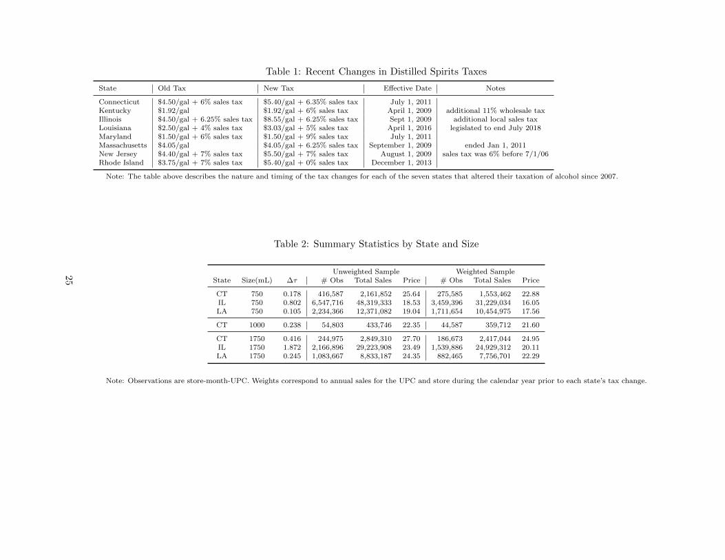
Table 1: Recent Changes in Distilled Spirits Taxes
State Old Tax New Tax Effective Date Notes
Connecticut $4.50/gal + 6% sales tax $5.40/gal + 6.35% sales tax July 1, 2011Kentucky $1.92/gal $1.92/gal + 6% sales tax April 1, 2009 additional 11% wholesale taxIllinois $4.50/gal + 6.25% sales tax $8.55/gal + 6.25% sales tax Sept 1, 2009 additional local sales taxLouisiana $2.50/gal + 4% sales tax $3.03/gal + 5% sales tax April 1, 2016 legislated to end July 2018Maryland $1.50/gal + 6% sales tax $1.50/gal + 9% sales tax July 1, 2011Massachusetts $4.05/gal $4.05/gal + 6.25% sales tax September 1, 2009 ended Jan 1, 2011New Jersey $4.40/gal + 7% sales tax $5.50/gal + 7% sales tax August 1, 2009 sales tax was 6% before 7/1/06Rhode Island $3.75/gal + 7% sales tax $5.40/gal + 0% sales tax December 1, 2013
Note: The table above describes the nature and timing of the tax changes for each of the seven states that altered their taxation of alcohol since 2007.
Table 2: Summary Statistics by State and Size
Unweighted Sample Weighted SampleState Size(mL) ∆τ # Obs Total Sales Price # Obs Total Sales Price
CT 750 0.178 416,587 2,161,852 25.64 275,585 1,553,462 22.88IL 750 0.802 6,547,716 48,319,333 18.53 3,459,396 31,229,034 16.05LA 750 0.105 2,234,366 12,371,082 19.04 1,711,654 10,454,975 17.56
CT 1000 0.238 54,803 433,746 22.35 44,587 359,712 21.60
CT 1750 0.416 244,975 2,849,310 27.70 186,673 2,417,044 24.95IL 1750 1.872 2,166,896 29,223,908 23.49 1,539,886 24,929,312 20.11LA 1750 0.245 1,083,667 8,833,187 24.35 882,465 7,756,701 22.29
Note: Observations are store-month-UPC. Weights correspond to annual sales for the UPC and store during the calendar year prior to each state’s tax change.
25
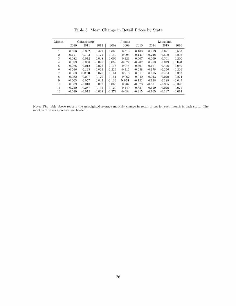
Table 3: Mean Change in Retail Prices by State
Month Connecticut Illinois Louisiana2010 2011 2012 2008 2009 2010 2014 2015 2016
1 0.326 0.382 0.429 0.606 0.518 0.108 0.499 0.621 0.5332 -0.127 -0.133 -0.122 0.149 -0.095 -0.147 -0.218 -0.509 -0.2363 -0.082 -0.072 0.048 -0.009 -0.121 -0.007 -0.059 0.391 0.2004 0.029 0.066 -0.028 0.039 -0.077 -0.207 0.288 0.049 0.1865 -0.076 0.012 0.026 -0.116 0.074 -0.601 -0.177 -0.446 -0.0496 -0.016 0.133 -0.003 -0.229 -0.412 -0.058 -0.178 -0.256 -0.2267 0.068 0.316 0.076 0.181 0.216 0.611 0.425 0.454 0.3538 -0.032 -0.007 0.170 0.151 -0.062 0.040 0.013 0.079 -0.2249 -0.005 0.057 0.043 -0.139 0.651 -0.121 0.128 0.189 -0.04910 0.039 -0.018 0.002 0.065 0.787 -0.073 -0.531 -0.305 -0.32011 -0.210 -0.287 -0.195 -0.120 0.140 -0.331 -0.129 0.076 -0.07112 -0.020 -0.072 -0.008 -0.374 -0.084 -0.215 -0.105 -0.197 -0.014
Note: The table above reports the unweighted average monthly change in retail prices for each month in each state. Themonths of taxes increases are bolded.
26

Table 4: Pass-Through: Taxes to Retail Prices
All Observations ∆ Retail Price 6= 01 month 3 month 6 month 1 month 3 month 6 month
Connecticut July 1, 2011 Tax Increase of $0.24/L
∆ Tax (750mL) 2.740∗ 2.816∗ 2.283∗ 5.824∗ 4.508∗ 3.393∗
(0.662) (0.509) (0.586) (1.500) (0.976) (1.147)∆ Tax (1000mL) 1.659∗ 1.841∗ 1.741∗ 3.291∗ 2.231∗ 2.007
(0.366) (0.434) (0.406) (1.170) (0.852) (0.854)∆ Tax (1750mL) 0.986∗ 0.802∗ 0.483∗ 1.997∗ 1.212 0.705
(0.291) (0.232) (0.259) (0.717) (0.484) (0.549)
Illinois Sept 1, 2009 Tax Increase of $1.07/L
∆ Tax (750mL) 0.655∗ 1.547∗ 2.007∗ 0.979∗ 1.982∗ 2.357∗
(0.125) (0.114) (0.094) (0.204) (0.156) (0.104)∆ Tax (1750mL) 0.401∗ 0.822∗ 0.858∗ 1.108∗ 1.150∗ 1.016∗
(0.053) (0.075) (0.114) (0.129) (0.099) (0.129)
Lousiana Sept 1, 2009 Tax Increase of $0.14/L
∆ Tax (750mL) 1.230 3.776∗ 1.685∗ 2.146 6.331∗ 0.612(0.942) (0.961) (0.916) (1.827) (1.497) (1.213)
∆ Tax (1750mL) 0.321 2.253∗ 0.683∗ 0.454 3.581∗ 0.142(0.508) (0.476) (0.400) (0.915) (0.692) (0.530)
Observations 7,049,524 6,859,112 6,678,483 2,821,502 3,759,221 4,239,584Adjusted R2 0.021 0.040 0.042 0.050 0.075 0.070
Note: The table above reports separate OLS estimates of the pass-through rate for each state. We include fixed effects forUPC, month of year, and year (all interacted with state). All regressions are weighted by annual sales for the UPC andstore during the calendar year prior to each state’s tax change. Standard errors are clustered at the state-UPC level. Weprovide quarterly results in Appendix Table C3.∗ Significant at the 1 percent level.
27

Table 5: Quarterly Retail Price Transitions by State, Cents Only
Connecticut
from/to 0.49 0.59 0.65 0.69 0.79 0.89 0.93 0.95 0.98 0.99 other
0.49 2.26 0.02 0.00 0.00 0.00 0.01 0.00 0.01 0.00 0.73 0.030.59 0.04 0.98 0.00 0.00 0.00 0.00 0.00 0.01 0.00 0.29 0.020.65 0.00 0.00 0.07 0.00 0.00 0.00 0.00 0.00 0.00 0.03 0.010.69 0.02 0.01 0.00 0.18 0.00 0.00 0.00 0.00 0.00 0.06 0.010.79 0.01 0.02 0.00 0.00 0.12 0.00 0.00 0.00 0.00 0.06 0.010.89 0.00 0.00 0.00 0.00 0.00 0.41 0.00 0.00 0.00 0.02 0.000.93 0.00 0.00 0.00 0.00 0.00 0.00 0.61 0.01 0.00 0.30 0.030.95 0.00 0.01 0.00 0.00 0.00 0.00 0.00 0.06 0.00 0.20 0.020.98 0.00 0.00 0.00 0.00 0.00 0.00 0.00 0.00 0.63 0.20 0.010.99 0.72 0.32 0.02 0.07 0.08 0.17 0.07 0.17 0.13 88.55 0.72other 0.03 0.02 0.01 0.01 0.01 0.01 0.03 0.01 0.01 0.82 0.49total 3.08 1.38 0.10 0.26 0.21 0.60 0.71 0.27 0.77 91.26 1.35ergodic 3.04 1.42 0.08 0.22 0.19 3.96 0.26 0.25 0.54 88.82 1.22
Illinois
from/to 0.19 0.29 0.39 0.49 0.59 0.79 0.89 0.97 0.98 0.99 other
0.19 0.06 0.00 0.00 0.02 0.00 0.01 0.00 0.00 0.00 0.25 0.040.29 0.00 0.15 0.00 0.03 0.00 0.01 0.00 0.00 0.00 0.18 0.030.39 0.00 0.00 0.07 0.02 0.00 0.01 0.00 0.00 0.00 0.30 0.040.49 0.02 0.04 0.03 2.03 0.02 0.06 0.02 0.03 0.01 2.14 0.380.59 0.01 0.00 0.00 0.03 0.11 0.01 0.00 0.00 0.00 0.28 0.040.79 0.01 0.01 0.01 0.05 0.01 0.23 0.01 0.00 0.00 0.65 0.070.89 0.00 0.00 0.00 0.02 0.00 0.01 0.07 0.00 0.00 0.22 0.030.97 0.00 0.00 0.00 0.01 0.00 0.01 0.00 3.24 0.00 1.29 0.090.98 0.00 0.00 0.00 0.01 0.00 0.00 0.00 0.01 1.07 0.07 0.150.99 0.19 0.16 0.27 2.14 0.24 0.61 0.20 1.43 0.12 71.43 3.09other 0.04 0.04 0.04 0.40 0.05 0.06 0.03 0.13 0.14 3.38 1.97total 0.33 0.40 0.42 4.76 0.43 1.02 0.33 4.84 1.34 80.19 5.93ergodic 0.31 0.39 0.41 4.68 0.41 1.00 0.32 5.28 1.41 80.02 5.77
Louisiana
from/to 0.19 0.29 0.39 0.49 0.59 0.69 0.79 0.89 0.95 0.99 other
0.19 0.48 0.01 0.01 0.02 0.01 0.02 0.01 0.01 0.00 0.10 0.030.29 0.01 0.76 0.02 0.04 0.01 0.01 0.02 0.01 0.00 0.13 0.020.39 0.01 0.02 0.61 0.04 0.01 0.02 0.02 0.01 0.00 0.16 0.030.49 0.03 0.05 0.05 5.75 0.06 0.06 0.05 0.08 0.01 2.98 0.230.59 0.01 0.01 0.01 0.04 0.67 0.02 0.02 0.01 0.00 0.12 0.020.69 0.01 0.01 0.02 0.07 0.02 0.80 0.03 0.01 0.00 0.12 0.020.79 0.01 0.01 0.02 0.07 0.01 0.02 0.68 0.02 0.00 0.13 0.020.89 0.01 0.01 0.02 0.07 0.01 0.02 0.02 0.74 0.00 0.10 0.030.95 0.00 0.00 0.00 0.03 0.00 0.00 0.00 0.00 1.19 0.46 0.370.99 0.15 0.22 0.23 3.02 0.20 0.21 0.21 0.20 0.70 71.53 1.40other 0.02 0.03 0.02 0.28 0.02 0.02 0.02 0.03 0.12 1.81 1.41total 0.74 1.13 1.01 9.43 1.02 1.20 1.08 1.12 2.02 77.64 3.58ergodic 0.89 1.48 1.26 9.61 1.33 1.56 1.41 1.42 1.90 75.69 3.46
Note: The table above reports the unweighted share of all prices accounted for by each transition type. The rows signifyfrom price endings while the columns signify to price endings. The total row at the bottom of each matrix reports the shareof prices at each price point. The most frequent transition pattern in each state is bolded along with the correspondingtotal share.
28

Table 6: Quarterly Retail Price Increments
All Weeks Month of Tax ChangeCT IL LA CT IL LA
Whole Dollar 71.08 61.57 64.75 75.96 67.15 63.72Half Dollar 6.59 8.61 13.25 6.20 8.83 12.12Small Change 2.72 4.91 3.11 1.12 1.60 2.04Large Change 4.11 1.71 1.97 2.38 1.46 1.87Other 15.50 23.19 16.92 14.33 20.96 20.25
Zeros 78.28 46.25 53.56 58.67 14.67 38.88
Note: The table above reports the unweighted share of quarterly price changes that are in whole dollar, half dollar andother increments. Price changes larger than $8 or smaller than $0.25 in magnitude are labelled Very Large and Very Small,respectively. No Change reports the share of prices that are unchanged.
Table 7: Ordered Logit Estimates ∆p ∈ −1, 0,+1,+2,+3Cubic Quartic Quintic Spline(1)
∆t 498.114∗ 523.324∗ 523.353∗ 1.841∗
(28.189) (28.034) (27.995) (0.535)∆t2 -104.691∗ -130.026∗ -129.352∗ -6.094
(27.446) (28.134) (28.172) (3.227)∆t3 -46.388∗ -28.202 -33.103 29.941∗
(16.433) (17.116) (18.926) (8.990)∆t4 -39.447∗ -32.614 3.220∗
(13.420) (17.393) (0.238)∆t5 -7.496
(14.520)
N 2,371,792 2,371,792 2,371,792 2,371,792# Clusters 3,567 3,567 3,567 3,567-LL 1,025,925 1,025,797 1,025,900 1,024,963BIC 2,052,727 2,052,498 2,052,731 2,050,829
∗ Significant at the 1 percent level. All standard errors are clustered at state-UPC level.Maximum Likelihood Estimates weighted by product sales in year prior to tax change.Weights balanced by state, bottle size, and tax change indicator.Orthogonal polynomials reported except for Spline.Spline has knot point at ∆τ = 1, spline coefficients are not polynomial order.
29
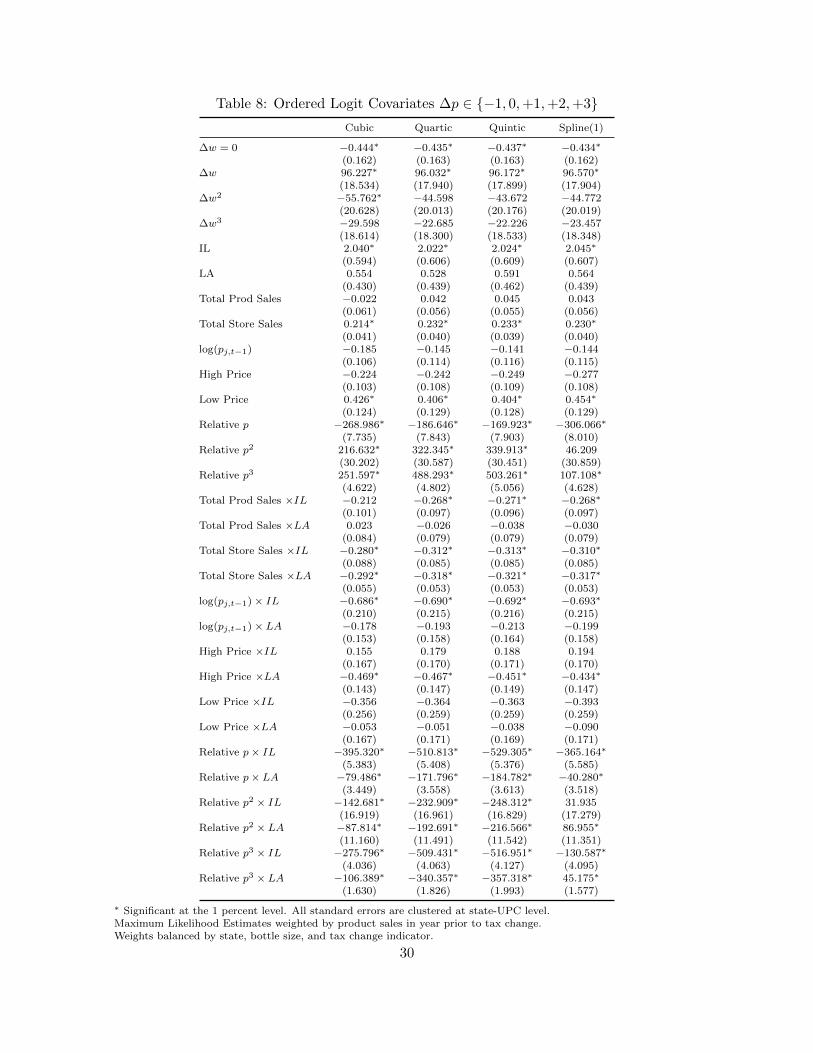
Table 8: Ordered Logit Covariates ∆p ∈ −1, 0,+1,+2,+3Cubic Quartic Quintic Spline(1)
∆w = 0 −0.444∗ −0.435∗ −0.437∗ −0.434∗
(0.162) (0.163) (0.163) (0.162)∆w 96.227∗ 96.032∗ 96.172∗ 96.570∗
(18.534) (17.940) (17.899) (17.904)∆w2 −55.762∗ −44.598 −43.672 −44.772
(20.628) (20.013) (20.176) (20.019)∆w3 −29.598 −22.685 −22.226 −23.457
(18.614) (18.300) (18.533) (18.348)IL 2.040∗ 2.022∗ 2.024∗ 2.045∗
(0.594) (0.606) (0.609) (0.607)LA 0.554 0.528 0.591 0.564
(0.430) (0.439) (0.462) (0.439)Total Prod Sales −0.022 0.042 0.045 0.043
(0.061) (0.056) (0.055) (0.056)Total Store Sales 0.214∗ 0.232∗ 0.233∗ 0.230∗
(0.041) (0.040) (0.039) (0.040)log(pj,t−1) −0.185 −0.145 −0.141 −0.144
(0.106) (0.114) (0.116) (0.115)High Price −0.224 −0.242 −0.249 −0.277
(0.103) (0.108) (0.109) (0.108)Low Price 0.426∗ 0.406∗ 0.404∗ 0.454∗
(0.124) (0.129) (0.128) (0.129)Relative p −268.986∗ −186.646∗ −169.923∗ −306.066∗
(7.735) (7.843) (7.903) (8.010)Relative p2 216.632∗ 322.345∗ 339.913∗ 46.209
(30.202) (30.587) (30.451) (30.859)Relative p3 251.597∗ 488.293∗ 503.261∗ 107.108∗
(4.622) (4.802) (5.056) (4.628)Total Prod Sales ×IL −0.212 −0.268∗ −0.271∗ −0.268∗
(0.101) (0.097) (0.096) (0.097)Total Prod Sales ×LA 0.023 −0.026 −0.038 −0.030
(0.084) (0.079) (0.079) (0.079)Total Store Sales ×IL −0.280∗ −0.312∗ −0.313∗ −0.310∗
(0.088) (0.085) (0.085) (0.085)Total Store Sales ×LA −0.292∗ −0.318∗ −0.321∗ −0.317∗
(0.055) (0.053) (0.053) (0.053)log(pj,t−1)× IL −0.686∗ −0.690∗ −0.692∗ −0.693∗
(0.210) (0.215) (0.216) (0.215)log(pj,t−1)× LA −0.178 −0.193 −0.213 −0.199
(0.153) (0.158) (0.164) (0.158)High Price ×IL 0.155 0.179 0.188 0.194
(0.167) (0.170) (0.171) (0.170)High Price ×LA −0.469∗ −0.467∗ −0.451∗ −0.434∗
(0.143) (0.147) (0.149) (0.147)Low Price ×IL −0.356 −0.364 −0.363 −0.393
(0.256) (0.259) (0.259) (0.259)Low Price ×LA −0.053 −0.051 −0.038 −0.090
(0.167) (0.171) (0.169) (0.171)Relative p× IL −395.320∗ −510.813∗ −529.305∗ −365.164∗
(5.383) (5.408) (5.376) (5.585)Relative p× LA −79.486∗ −171.796∗ −184.782∗ −40.280∗
(3.449) (3.558) (3.613) (3.518)Relative p2 × IL −142.681∗ −232.909∗ −248.312∗ 31.935
(16.919) (16.961) (16.829) (17.279)Relative p2 × LA −87.814∗ −192.691∗ −216.566∗ 86.955∗
(11.160) (11.491) (11.542) (11.351)Relative p3 × IL −275.796∗ −509.431∗ −516.951∗ −130.587∗
(4.036) (4.063) (4.127) (4.095)Relative p3 × LA −106.389∗ −340.357∗ −357.318∗ 45.175∗
(1.630) (1.826) (1.993) (1.577)
∗ Significant at the 1 percent level. All standard errors are clustered at state-UPC level.Maximum Likelihood Estimates weighted by product sales in year prior to tax change.Weights balanced by state, bottle size, and tax change indicator.
30
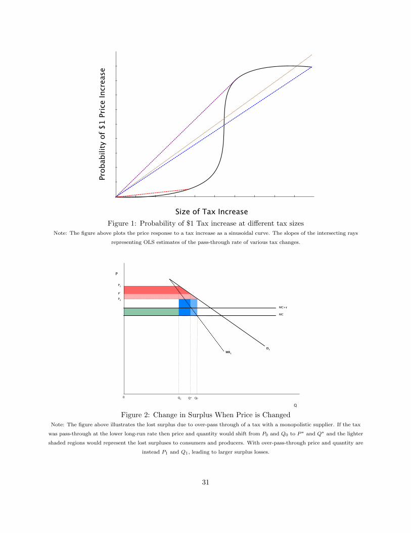
Size of Tax Increase
Prob
abili
ty o
f $1
Pric
e In
crea
se
Figure 1: Probability of $1 Tax increase at different tax sizesNote: The figure above plots the price response to a tax increase as a sinusoidal curve. The slopes of the intersecting rays
representing OLS estimates of the pass-through rate of various tax changes.
0
Q
D1MR1
P
Q0Q*
MC
P*
MC+𝝉
P0
P1
Q1
Figure 2: Change in Surplus When Price is ChangedNote: The figure above illustrates the lost surplus due to over-pass through of a tax with a monopolistic supplier. If the tax
was pass-through at the lower long-run rate then price and quantity would shift from P0 and Q0 to P ∗ and Q∗ and the lighter
shaded regions would represent the lost surpluses to consumers and producers. With over-pass-through price and quantity are
instead P1 and Q1, leading to larger surplus losses.
31

Figure 3: Frequency of Retail Price AdjustmentsNote: The figure above plots the share of retail prices that change and that increase in each state for each month between
2007 and 2016, weighted by annual sales for the UPC and store in the calendar year prior to each state’s tax change, balanced
on package size.
32

Figure 4: Pass-Through EstimatesNote: The first figure above plots the estimated pass-through rates for different size tax increases. The second figure plots the
pass-through estimates conditional on a price change. All regressions are weighted by annual sales for the UPC and store
during the calendar year prior to each state’s tax change, normalized by size and state. The dashed lines estimate the
pass-through rates as linear functions of the tax. For the unconditional left panel the parameters of the best fit line are:
ρ(∆τ) = 1.76− 0.51 ∗∆τ while for the conditional right panel the best fit line is ρ(∆τ) = 2.47− 0.72 ∗∆τ . The dotted lines
indicate the implied pass through of a $1.00 and $2.00 price change respectively.
33

Figure 5: Specification Comparison for Ordered LogitTop Pane: Predicted Price Change; Bottom Pane: Implied Pass Through Rate.
Vertical Lines at Observed Tax Changes.
34

Figure 6: Welfare Predictions: Ordered Logit vs. OLS (Own Elasticity ε = −3.5)Top Pane: Effieciency: DWL per Dollar of Tax Revenue; Bottom Pane: Incidence ∆CS/∆PS.
Vertical Lines at Observed Tax Changes.
35

Figure 7: Welfare Predictions: Alternate ElasticitiesVertical Lines at Observed Tax Changes
36
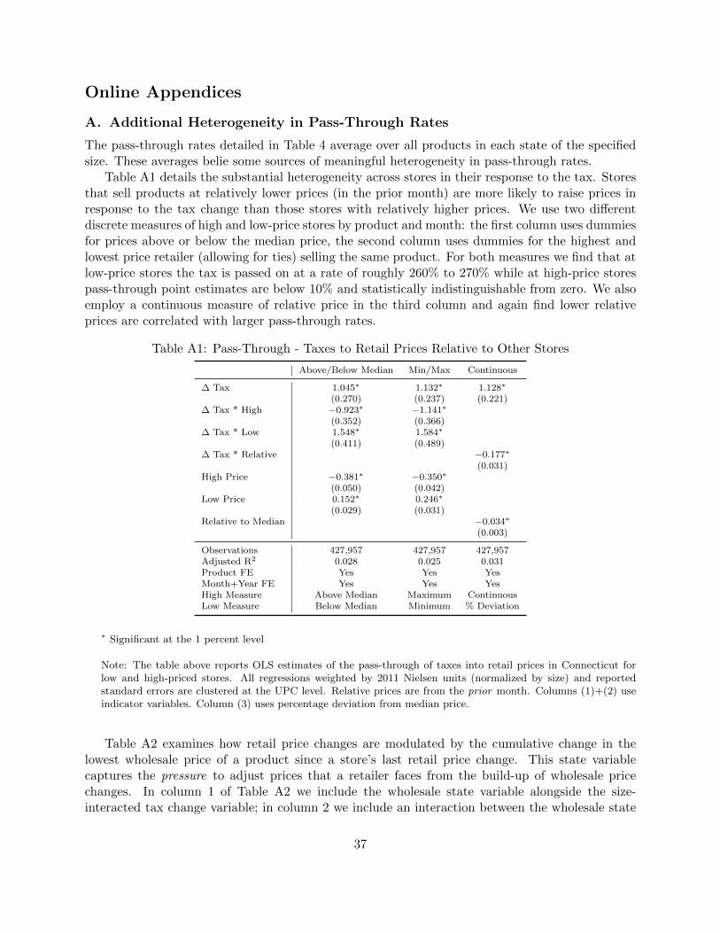
Online Appendices
A. Additional Heterogeneity in Pass-Through Rates
The pass-through rates detailed in Table 4 average over all products in each state of the specifiedsize. These averages belie some sources of meaningful heterogeneity in pass-through rates.
Table A1 details the substantial heterogeneity across stores in their response to the tax. Storesthat sell products at relatively lower prices (in the prior month) are more likely to raise prices inresponse to the tax change than those stores with relatively higher prices. We use two differentdiscrete measures of high and low-price stores by product and month: the first column uses dummiesfor prices above or below the median price, the second column uses dummies for the highest andlowest price retailer (allowing for ties) selling the same product. For both measures we find that atlow-price stores the tax is passed on at a rate of roughly 260% to 270% while at high-price storespass-through point estimates are below 10% and statistically indistinguishable from zero. We alsoemploy a continuous measure of relative price in the third column and again find lower relativeprices are correlated with larger pass-through rates.
Table A1: Pass-Through - Taxes to Retail Prices Relative to Other Stores
Above/Below Median Min/Max Continuous
∆ Tax 1.045∗ 1.132∗ 1.128∗
(0.270) (0.237) (0.221)∆ Tax * High −0.923∗ −1.141∗
(0.352) (0.366)∆ Tax * Low 1.548∗ 1.584∗
(0.411) (0.489)∆ Tax * Relative −0.177∗
(0.031)High Price −0.381∗ −0.350∗
(0.050) (0.042)Low Price 0.152∗ 0.246∗
(0.029) (0.031)Relative to Median −0.034∗
(0.003)
Observations 427,957 427,957 427,957Adjusted R2 0.028 0.025 0.031Product FE Yes Yes YesMonth+Year FE Yes Yes YesHigh Measure Above Median Maximum ContinuousLow Measure Below Median Minimum % Deviation
∗ Significant at the 1 percent level
Note: The table above reports OLS estimates of the pass-through of taxes into retail prices in Connecticut forlow and high-priced stores. All regressions weighted by 2011 Nielsen units (normalized by size) and reportedstandard errors are clustered at the UPC level. Relative prices are from the prior month. Columns (1)+(2) useindicator variables. Column (3) uses percentage deviation from median price.
Table A2 examines how retail price changes are modulated by the cumulative change in thelowest wholesale price of a product since a store’s last retail price change. This state variablecaptures the pressure to adjust prices that a retailer faces from the build-up of wholesale pricechanges. In column 1 of Table A2 we include the wholesale state variable alongside the size-interacted tax change variable; in column 2 we include an interaction between the wholesale state
37

variable and the change in tax and in column 3 we include both the main and interaction terms.In all specifications larger cumulative changes in wholesale prices since the last retail price changelead to larger retail price increases. While the main effect and interaction term are statisticallysignificant on their own (columns 1 and 2) when both are included only the main effect of thewholesale state variable is significant though the point estimate of the interaction term is of theexpected positive sign.
Table A2: Pass-Through - Adding Wholesale Price Change State Variable (CT only)
(1) (2) (3)
∆ Tax (750mL) 2.949∗ 3.028∗ 2.887∗
(0.815) (0.818) (0.820)∆ Tax (1000mL) 2.024∗ 2.014∗ 1.953∗
(0.575) (0.581) (0.581)∆ Tax (1750mL) 0.672∗ 0.510 0.592
(0.391) (0.404) (0.402)∆W 0.107∗ 0.106∗
(0.018) (0.019)∆W ×∆T 0.394∗ 0.092
(0.105) (0.109)
Observations 92,553 92,553 92,553Adjusted R2 0.040 0.022 0.040
∗ Significant at the 1 percent level.Note: The table above reports quarterly OLS estimates of the pass-through of taxes into retail prices inConnecticut controlling for the change in the product’s wholesale price since the last change in the store’s retailprice for that product. All regressions weighted by 2010 Nielsen units (normalized by size) and reported standarderrors are clustered at the UPC level.
B. Data
B.1. Aggregation of Nielsen Weekly Data to Monthly Data
The Nielsen scanner data are recorded weekly, and some weeks span two months. We aggregatethe data to the monthly level for the initial analysis for a number of reasons. The first is thatin Connecticut, wholesale (and retail) prices are not allowed to vary within a month. This isnot necessarily true in Illinois or Louisiana where prices can adjust more flexibly. Second, whentax changes are observed, the occur on the first day of the month. We allocate weeks to monthsbased on the calendar month of the last day of the corresponding week. When we aggregate, wetake the last price (Nielsen revenue divided by units) recorded in each month and total sales foreach product-store-month. In practice, there is only a single price for 99% of store-month-productobservations in Connecticut once we exclude the first week of the month (which may contain datafrom two months).
B.2. Consolidation
We consolidate products so that a product is defined as brand-flavor-size such as Smirnoff OrangeVodka 750mL. Sometimes a “product” may aggregate over several UPC’s, as changes in packagingcan result in a new UPC. UPC changes most commonly arise with special promotional packagingsuch as a commemorative bottle, or a holiday gift set. At other times, the change in UPC maybe purely temporal in nature. A product may also be available in both glass and plastic bottles
38

at the same time. We rarely observe price differences for glass and plastic packaging within aproduct-month, so we also consolidate these UPCs.
In total, these consolidations help us to construct a more balanced panel of products over time,and avoid gaps during holiday periods, or products going missing when packaging changes. Thisis especially important when our goal is to capture changes in prices within a product-store overtime.
B.3. Cleaning Prices
Nielsen data report weekly sales at the store-UPC level. Prices are not observed directly but ratherimputed from revenues as pt ≈ pt·qt
qt. It is common to adjust or filter prices under a number of
scenarios: (1) transitional prices (2) temporary sales (3) clearance/closeouts. For (1) observedprices may not represent transaction prices, but rather the weighted average of two different pricepoints. For (2) and (3) the observed prices may in fact be transaction prices, but those pricesmay not end in 0.99 as many stores/chains use unusual price endings internally to track sales orclearances.
It is helpful to consider a sequence of prices for a product [pt−2, pt−1, pt, pt+1, pt+1] and so on.In many cases pt and pt+1 are not adjacent weeks but rather adjacent periods in which a sale isrecorded. This is is important because Nielsen does not record any information unless a productwas purchased that week.
Rule #1: Transitional Prices
If the store changes its prices at the end of a Nielsen-week (Saturday to Saturday) the the recordedprice should match the actual transaction price. A more likely scenario is that a store changesits price midweek so that revenues include sales recorded at pt−1 and pt+1, while no transactionsactually take place at the recorded pt. Because we are interested in price changes we will replacept with the closer of pt−1, pt+1, so that our recorded price corresponds to an actual transacted price(rather than a weighted average).
We can detect these transitional prices by when pt ∈ (pt−1, pt+1, ) or pt ∈ (pt+1, pt−1, ) and thenwe use observed sales qt to construct a convex set of potential prices where w = [1, . . . , qt − 1]/qtand pt ≈ wpt−1 + (1− w)pt+1 to see if pt lies on the grid of transitional prices.
We apply this rule only to price endings not in the four most commonly used price endings foreach chain in our dataset.
We include the code below:
def transition_prices(p1,p2,pobs,q):
# is observed price between (p1,p2)
if not (((pobs < p1) & (pobs > p2)) | ((pobs > p1) & (pobs < p2))):
return np.nan
#convex weights
w=np.array([x/q for x in range(0,q+1)])
# grid of possible prices
possible=w*p1 + (1-w)*p2
# check if observed price is within 1 cent of rounded grid of possible prices
# then return the closer price --> otherwise missing
if any(np.isclose(pobs,np.round(possible,3),atol=.01)):
if np.abs(p1-pobs) <= np.abs(p2-pobs):
return p1
else:
return p2
else:
return np.nan
39
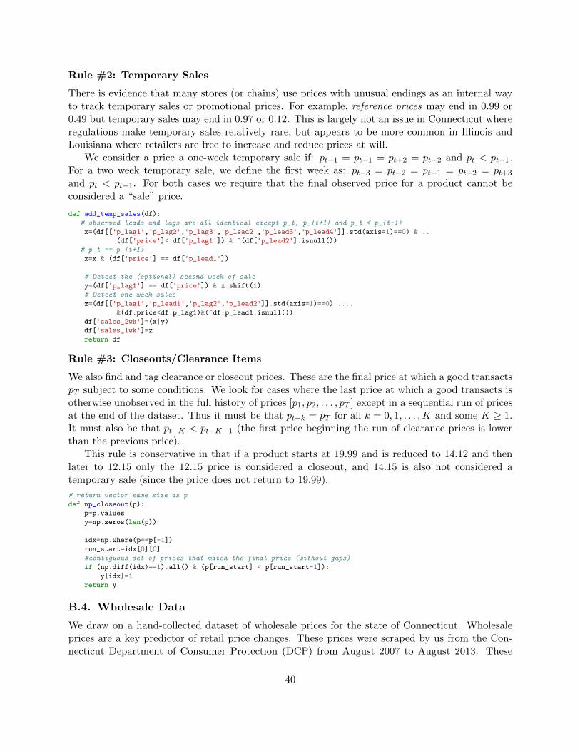
Rule #2: Temporary Sales
There is evidence that many stores (or chains) use prices with unusual endings as an internal wayto track temporary sales or promotional prices. For example, reference prices may end in 0.99 or0.49 but temporary sales may end in 0.97 or 0.12. This is largely not an issue in Connecticut whereregulations make temporary sales relatively rare, but appears to be more common in Illinois andLouisiana where retailers are free to increase and reduce prices at will.
We consider a price a one-week temporary sale if: pt−1 = pt+1 = pt+2 = pt−2 and pt < pt−1.For a two week temporary sale, we define the first week as: pt−3 = pt−2 = pt−1 = pt+2 = pt+3
and pt < pt−1. For both cases we require that the final observed price for a product cannot beconsidered a “sale” price.
def add_temp_sales(df):
# observed leads and lags are all identical except p_t, p_t+1 and p_t < p_t-1
x=(df[['p_lag1','p_lag2','p_lag3','p_lead2','p_lead3','p_lead4']].std(axis=1)==0) & ...
(df['price']< df['p_lag1']) & ~(df['p_lead2'].isnull())
# p_t == p_t+1
x=x & (df['price'] == df['p_lead1'])
# Detect the (optional) second week of sale
y=(df['p_lag1'] == df['price']) & x.shift(1)
# Detect one week sales
z=(df[['p_lag1','p_lead1','p_lag2','p_lead2']].std(axis=1)==0) ....
&(df.price<df.p_lag1)&(~df.p_lead1.isnull())
df['sales_2wk']=(x|y)
df['sales_1wk']=z
return df
Rule #3: Closeouts/Clearance Items
We also find and tag clearance or closeout prices. These are the final price at which a good transactspT subject to some conditions. We look for cases where the last price at which a good transacts isotherwise unobserved in the full history of prices [p1, p2, . . . , pT ] except in a sequential run of pricesat the end of the dataset. Thus it must be that pt−k = pT for all k = 0, 1, . . . ,K and some K ≥ 1.It must also be that pt−K < pt−K−1 (the first price beginning the run of clearance prices is lowerthan the previous price).
This rule is conservative in that if a product starts at 19.99 and is reduced to 14.12 and thenlater to 12.15 only the 12.15 price is considered a closeout, and 14.15 is also not considered atemporary sale (since the price does not return to 19.99).
# return vector same size as p
def np_closeout(p):
p=p.values
y=np.zeros(len(p))
idx=np.where(p==p[-1])
run_start=idx[0][0]
#contiguous set of prices that match the final price (without gaps)
if (np.diff(idx)==1).all() & (p[run_start] < p[run_start-1]):
y[idx]=1
return y
B.4. Wholesale Data
We draw on a hand-collected dataset of wholesale prices for the state of Connecticut. Wholesaleprices are a key predictor of retail price changes. These prices were scraped by us from the Con-necticut Department of Consumer Protection (DCP) from August 2007 to August 2013. These
40

data are available because Connecticut requires that all licensed wholesalers post prices. Whole-salers agree to charge retailers these prices for the entire month, and are legally not allowed toprovide quantity discounts or price discriminate.39 Only 18 wholesale firms have ever sold brandsof distilled spirits that we observe in the Nielsen dataset, and more than 80% of sales come fromjust six major wholesalers. Because Illinois and Louisiana do not require that wholesalers publiclypost prices, we do not have wholesale pricing information for these states.
For our welfare calculations we use estimates from Conlon and Rao (2015) of the prices paidby wholesale firms to importers and distillers. These marginal costs are estimated at the productlevel using a structural model of demand in the approach of Berry et al. (2004).
C. Quarterly Pass-Through and Price Points
C.1. Constructing Quarterly Data
We estimate our nonlinear models using quarterly data to avoid the repetitive use of monthlyobservations. We allocate weeks to quarters using the last day of each week. This works forConnecticut where the tax changes on July 1 (the first day of Q3), and Louisiana where the taxchanges on April 1 (the first day of Q2). We have to modify this procedure for Illinois, where thetax changes on September 1. For Illinois, we change the starting month for each quarter so that Q1begins in December, Q2 begins in March, Q3 begins in June, and Q4 begins in September. Thisway, the tax change happens at the beginning of of Q4 under our adjusted definition.40 When weaggregate, we take the last price (Nielsen revenue divided by units) recorded in each quarter andtotal sales for each product-store-quarter.
For comparison, in the left panel of Table C3 we reproduce Table 4 from the main text using thequarterly data instead of monthly data. We find that the patterns are broadly similar, though wehave fewer observations, larger standard errors, and less precise control over seasonality. In all butonce case (1750mL bottles in Connecticut) we find evidence that taxes are over-shifted ρ > 1 andthat conditional on a price change, estimated pass-through rates are higher. The latter effects aremuted as one might expect because at the quarterly level price changes are more common overall.
39Connecticut is one of 12 states with a set of regulations known as Post and Hold, which mandates that allwholesalers post the prices they plan to charge retailers for the following month. Wholesalers must commit tocharging these prices for the entire month (after a look-back period when wholesalers can view one another’s initiallyposted prices and adjust their prices downwards without beating the lowest price for the product). For a detailedanalysis of these regulations please see Conlon and Rao (2015).
40These definitions make it difficult to include quarterly fixed effects in regression specifications, as December (ahigh sales month) is in Q4 for (CT,LA) and Q1 in IL. For this reason we only ever consider State × Quarter fixedeffects.
41
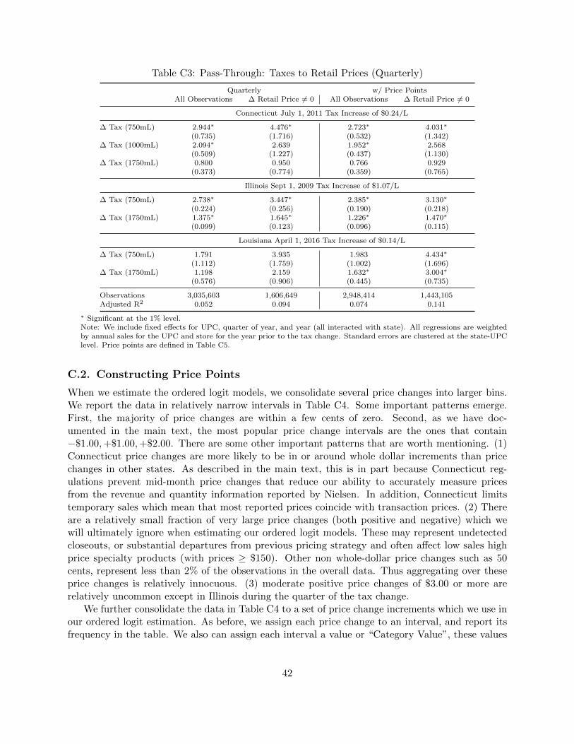
Table C3: Pass-Through: Taxes to Retail Prices (Quarterly)
Quarterly w/ Price PointsAll Observations ∆ Retail Price 6= 0 All Observations ∆ Retail Price 6= 0
Connecticut July 1, 2011 Tax Increase of $0.24/L
∆ Tax (750mL) 2.944∗ 4.476∗ 2.723∗ 4.031∗
(0.735) (1.716) (0.532) (1.342)∆ Tax (1000mL) 2.094∗ 2.639 1.952∗ 2.568
(0.509) (1.227) (0.437) (1.130)∆ Tax (1750mL) 0.800 0.950 0.766 0.929
(0.373) (0.774) (0.359) (0.765)
Illinois Sept 1, 2009 Tax Increase of $1.07/L
∆ Tax (750mL) 2.738∗ 3.447∗ 2.385∗ 3.130∗
(0.224) (0.256) (0.190) (0.218)∆ Tax (1750mL) 1.375∗ 1.645∗ 1.226∗ 1.470∗
(0.099) (0.123) (0.096) (0.115)
Louisiana April 1, 2016 Tax Increase of $0.14/L
∆ Tax (750mL) 1.791 3.935 1.983 4.434∗
(1.112) (1.759) (1.002) (1.696)∆ Tax (1750mL) 1.198 2.159 1.632∗ 3.004∗
(0.576) (0.906) (0.445) (0.735)
Observations 3,035,603 1,606,649 2,948,414 1,443,105Adjusted R2 0.052 0.094 0.074 0.141
∗ Significant at the 1% level.Note: We include fixed effects for UPC, quarter of year, and year (all interacted with state). All regressions are weightedby annual sales for the UPC and store for the year prior to the tax change. Standard errors are clustered at the state-UPClevel. Price points are defined in Table C5.
C.2. Constructing Price Points
When we estimate the ordered logit models, we consolidate several price changes into larger bins.We report the data in relatively narrow intervals in Table C4. Some important patterns emerge.First, the majority of price changes are within a few cents of zero. Second, as we have doc-umented in the main text, the most popular price change intervals are the ones that contain−$1.00,+$1.00,+$2.00. There are some other important patterns that are worth mentioning. (1)Connecticut price changes are more likely to be in or around whole dollar increments than pricechanges in other states. As described in the main text, this is in part because Connecticut reg-ulations prevent mid-month price changes that reduce our ability to accurately measure pricesfrom the revenue and quantity information reported by Nielsen. In addition, Connecticut limitstemporary sales which mean that most reported prices coincide with transaction prices. (2) Thereare a relatively small fraction of very large price changes (both positive and negative) which wewill ultimately ignore when estimating our ordered logit models. These may represent undetectedcloseouts, or substantial departures from previous pricing strategy and often affect low sales highprice specialty products (with prices ≥ $150). Other non whole-dollar price changes such as 50cents, represent less than 2% of the observations in the overall data. Thus aggregating over theseprice changes is relatively innocuous. (3) moderate positive price changes of $3.00 or more arerelatively uncommon except in Illinois during the quarter of the tax change.
We further consolidate the data in Table C4 to a set of price change increments which we use inour ordered logit estimation. As before, we assign each price change to an interval, and report itsfrequency in the table. We also can assign each interval a value or “Category Value”, these values
42

Table C4: Frequency of Quarterly Price Change Intervals
All Quarters Quarter of Tax ChangePrice Change CT IL LA CT IL LA
(-10,-6.03] 0.51 0.85 0.57 0.30 0.82 0.74(-6.03,-5.97] 0.18 0.36 0.31 0.11 0.24 0.44(-5.97,-5.03] 0.092 0.25 0.15 0.12 0.16 0.33(-5.03,-4.97] 0.31 0.60 0.64 0.44 0.30 0.77(-4.97,-4.03] 0.11 0.48 0.25 0.03 0.33 0.38
(-4.03,-3.97] 0.57 1.11 1.26 0.62 0.90 1.67(-3.97,-3.03] 0.19 0.81 0.49 0.21 0.54 0.57(-3.03,-2.97] 0.86 2.25 2.14 0.84 1.48 2.26(-2.97,-2.03] 0.33 1.37 1.00 0.20 0.85 1.47(-2.03,-1.97] 1.50 4.84 3.95 1.63 0.94 4.01
(-1.97,-1.03] 0.44 2.29 1.86 0.44 1.16 2.77(-1.03,-0.97] 1.85 8.03 6.70 4.22 3.63 7.93(-0.97,-0.53] 0.15 1.24 0.93 0.14 0.67 0.90(-0.53,-0.47] 0.10 1.08 1.23 0.14 0.56 1.28(-0.47,-0.03] 0.28 1.57 1.22 0.45 0.91 1.38
(-0.03,0.03] 77.45 43.55 50.73 58.18 14.60 38.77
(0.03,0.47] 0.71 1.64 1.60 0.81 1.54 1.34(0.47,0.53] 0.63 1.30 1.92 1.30 1.23 3.72(0.53,0.97] 0.41 1.31 0.97 1.48 1.72 1.11(0.97,1.03] 5.88 9.32 8.28 14.85 13.46 11.93
(1.03,1.97] 0.62 2.42 2.18 1.42 6.52 3.06(1.97,2.03] 2.35 4.92 4.29 4.46 16.25 4.95(2.03,2.97] 0.36 1.43 1.10 0.89 4.92 0.99(2.97,3.03] 1.10 2.36 2.22 1.87 9.66 2.69(3.03,3.97] 0.23 0.70 0.46 0.48 2.45 0.47
(3.97,4.03] 0.72 1.13 1.07 1.40 4.07 1.27(4.03,4.97] 0.15 0.40 0.23 0.54 1.35 0.42(4.97,5.03] 0.42 0.69 0.74 0.65 4.22 0.60(5.03,5.97] 0.059 0.22 0.13 0.20 1.10 0.081(5.97,6.03] 0.23 0.37 0.31 0.35 0.96 0.38
(6.03,6.97] 0.056 0.12 0.071 0.11 0.32 0.062(6.97,7.03] 0.14 0.22 0.16 0.075 0.56 0.18(7.03,10] 0.39 0.31 0.29 0.30 0.75 0.36|∆P | > 10 0.60 0.46 0.53 0.75 0.81 0.70
43

are not used in the ordered logit estimation, however we do use these values when calculating ourcounterfactuals.
We estimate quarterly pass-through regressions using these transformed values and comparethe results to the un-transformed quarterly data in Table C3. The right panel of Table C3 confirmsthat transforming the data this way has little impact on the estimated pass-through rates. In allcases pass-through estimates using the transformed data are statistically indistinguishable from thequarterly pass-through estimates using the un-transformed data.
Table C5: Frequency of Quarterly Price Changes with Price Points
All Periods During Tax ChangeCategory Value Interval CT IL LA CT IL LA
-2 (-5.1,-1.5] 4.11 12.78 10.90 4.19 6.10 12.74-1 (-1.5,-0.25] 2.43 12.12 10.17 5.02 5.67 12.270 (-0.25,0.25] 77.97 45.23 52.32 58.68 16.04 40.03
+ 12
(0.25,0.75] 1.31 2.71 3.07 2.94 2.81 5.22+1 (0.75,1.5] 6.45 11.59 10.38 16.27 18.29 14.52
+2 (1.5,2.5] 2.74 6.64 5.67 5.41 21.98 6.45+3 (2.5,3.5] 1.40 3.29 2.81 2.35 12.86 3.28+4 (3.5,4.5] 0.89 1.63 1.37 2.05 5.91 1.72+5 (4.5,5.1] 0.47 0.86 0.82 0.78 4.65 0.67
|∆P | > 5.1 2.23 3.14 2.50 2.29 5.69 3.11
We can also look at how incorporating additional price points affects our estimates of predictedprice changes and pass-through in the ordered logit specification. We use the same quartic poly-nomial in ∆τ as before, but now instead of restricting ∆p ∈ ≤ −1, 0, 1, 2,≥ 3, we allow foradditional price points at ∆p ∈ +0.5 in one specification and further adds ∆p ∈ −2,+4 inanother. We report the results for predicted price changes in Figure C1. We find that adding theadditional price point at fifty cents has a negligible effect on our predicted price changes, and thatadding the additional price points at −2,+4, leads to slightly lower predictions for small taxchanges (because of the −2) and slightly higher predictions for large tax changes (because of the+4). The overall qualitative patterns are preserved. We prefer to consolidate the +$4,+$5 pricechanges with the +$3 price change because outside of Illinois during the month of the tax changethey are very rare and thus difficult to predict accurately.
C.3. Additional Robustness Tests
Here we consider additional robustness tests.We vary the elasticity of demand used to calculate counterfactual welfare: deadweight loss,
producer surplus, consumer surplus, tax revenue, and incidence. We replicate Figure 6 but insteaduse elasticities εd ∈ −2.5,−4.5. These are meant to capture the range of product-level own priceelasticities reported in the empirical literature. See Conlon and Rao (2015) or Miravete et al. (2018).We provide those results in Figures C2, C3. As we might expect, as we increase the elasticity ofdemand, consumers bear less of the burden and firms bear more. The social cost of taxationresponds the opposite way in that as demand becomes more elastic, ∆DWL increases. For the lesselastic demand, the linear pass-through estimate lies strictly above the price points/ordered logitestimates, and for more elastic demand it lies (partly) slightly below. In both cases the qualitativepatterns remain similar. Both the efficiency and incidence calculations produce a series of U-shapedcurves as we increase the size of the tax that qualitatively match our main result.
44
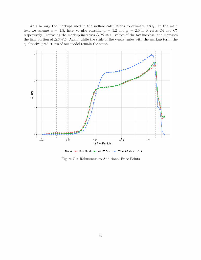
We also vary the markups used in the welfare calculations to estimate MCj . In the maintext we assume µ = 1.5, here we also consider µ = 1.2 and µ = 2.0 in Figures C4 and C5respectively. Increasing the markup increases ∆PS at all values of the tax increase, and increasesthe firm portion of ∆DWL. Again, while the scale of the y-axis varies with the markup term, thequalitative predictions of our model remain the same.
Figure C1: Robustness to Additional Price Points
45

Figure C2: Welfare Predictions: Ordered Logit vs. OLSTop Pane: Effieciency: DWL per Dollar of Tax Revenue; Bottom Pane: Incidence ∆CS/∆PS.
Own Elasticity ε = −2.5
Vertical Lines at Observed Tax Changes.
46

Figure C3: Welfare Predictions: Ordered Logit vs. OLSTop Pane: Effieciency: DWL per Dollar of Tax Revenue; Bottom Pane: Incidence ∆CS/∆PS.
Own Elasticity ε = −4.5
Vertical Lines at Observed Tax Changes.
47

Figure C4: Alternative Markups µ = 1.2: Ordered Logit vs. OLSTop Pane: Effieciency: DWL per Dollar of Tax Revenue; Bottom Pane: Incidence ∆CS/∆PS.
Own Elasticity ε = −3.5
Vertical Lines at Observed Tax Changes.
48

Figure C5: Alternative Markups µ = 2: Ordered Logit vs. OLSTop Pane: Effieciency: DWL per Dollar of Tax Revenue; Bottom Pane: Incidence ∆CS/∆PS.
Own Elasticity ε = −3.5
Vertical Lines at Observed Tax Changes.
49
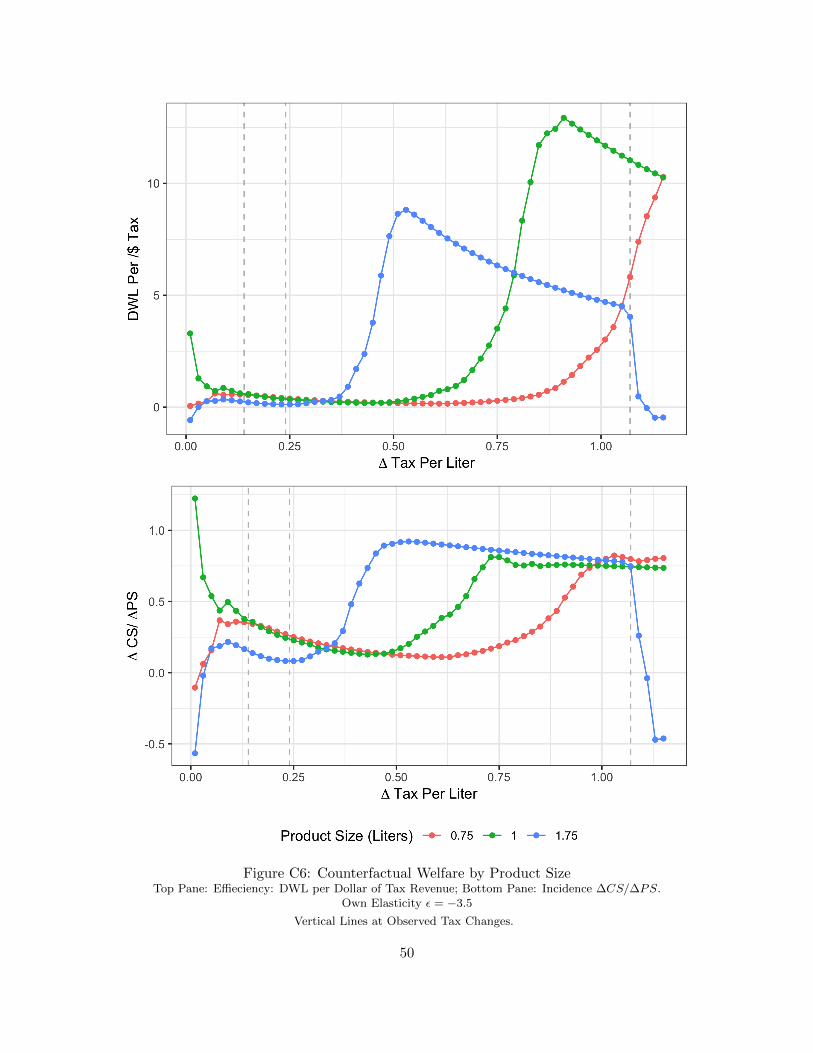
Figure C6: Counterfactual Welfare by Product SizeTop Pane: Effieciency: DWL per Dollar of Tax Revenue; Bottom Pane: Incidence ∆CS/∆PS.
Own Elasticity ε = −3.5
Vertical Lines at Observed Tax Changes.
50


