
University of Nebraska - Lincoln University of Nebraska - Lincoln
DigitalCommons@University of Nebraska - Lincoln DigitalCommons@University of Nebraska - Lincoln
Publications, Agencies and Staff of the U.S. Department of Commerce U.S. Department of Commerce
2011
High species density patterns in macrofaunal invertebrate High species density patterns in macrofaunal invertebrate
communities in the marine benthos communities in the marine benthos
John Oliver Moss Landing Marine Laboratories
Kamille Hammerstrom Moss Landing Marine Laboratories, [email protected]
Erika McPhee-Shaw Moss Landing Marine Laboratories
Peter Slattery Moss Landing Marine Laboratories
James Oakden Moss Landing Marine Laboratories
See next page for additional authors
Follow this and additional works at: https://digitalcommons.unl.edu/usdeptcommercepub
Part of the Environmental Sciences Commons
Oliver, John; Hammerstrom, Kamille; McPhee-Shaw, Erika; Slattery, Peter; Oakden, James; Kim, Stacy; and Hartwell, S. Ian, "High species density patterns in macrofaunal invertebrate communities in the marine benthos" (2011). Publications, Agencies and Staff of the U.S. Department of Commerce. 300. https://digitalcommons.unl.edu/usdeptcommercepub/300
This Article is brought to you for free and open access by the U.S. Department of Commerce at DigitalCommons@University of Nebraska - Lincoln. It has been accepted for inclusion in Publications, Agencies and Staff of the U.S. Department of Commerce by an authorized administrator of DigitalCommons@University of Nebraska - Lincoln.
Authors Authors John Oliver, Kamille Hammerstrom, Erika McPhee-Shaw, Peter Slattery, James Oakden, Stacy Kim, and S. Ian Hartwell
This article is available at DigitalCommons@University of Nebraska - Lincoln: https://digitalcommons.unl.edu/usdeptcommercepub/300
SPECIAL TOPIC
High species density patterns in macrofaunal invertebratecommunities in the marine benthosJohn Oliver1, Kamille Hammerstrom1, Erika McPhee-Shaw1, Peter Slattery1, James Oakden1, StacyKim1 & S. Ian Hartwell2
1 Moss Landing Marine Laboratories, Moss Landing, CA, USA
2 NOAA, Center for Coastal Monitoring & Assessment, Silver Spring, MO, USA
Introduction
Early ecologists wanted a term, or index, for species
diversity that could reflect the complexity of biological
interactions in a community and searched for models to
embody this concept, settling on the idea that a commu-
nity with a more even distribution of individuals among
species allowed for a greater probability of interspecific
encounters and was therefore more diverse. They bor-
rowed the Shannon–Wiener (Weaver) equation (H’) from
information theory with a questionable analogy to inter-
specific encounter (Goodman 1975). H’ became the most
commonly cited measure of species diversity. Goodman
(1975) reviewed the history of this measure and put into
words what it does to the number of species and individ-
uals: ‘The Shannon–Weaver measure of species diversity
is the negative logarithm of the geometric mean of the
probability per individual of correctly guessing, in
sequence, the species identity of each individual in a
random ordering of an assortment of individuals whose
relative species frequencies are given by {p1}, when the
‘guess’ is carried out by picking some arbitrary ordering
of this assortment of individuals’. He concluded: ‘It is a
dubious index. Whatever the index does measure seems
to have no direct biological interpretation’. The measure
of evenness (J), derived from H’, suffers from the same
problem. Hurlbert (1971) thought that the effort to repre-
sent the complexity of interactions in an encounter index
and the use of H’ rendered species diversity a noncon-
cept. He provided a realistic index of the probability of
interspecific encounter (PIE), which H’ was supposed to
be, but was not. Hurlbert urged that PIE not be used as
another measure of species diversity, but instead be
called what it was, an index of interspecific encounter.
Keywords
Diversity; dominance; infauna; marine
benthos; species density; species-area
relationships.
Correspondence
Kamille K. Hammerstrom, Moss Landing
Marine Laboratories, 8272 Moss Landing
Road, Moss Landing, CA, USA 95039.
E-mail: [email protected]
Accepted: 4 May 2011
doi:10.1111/j.1439-0485.2011.00461.x
Abstract
Species density of macrofaunal invertebrates living in marine soft sediments
was highest at the shelf-slope break (100–150 m) in Monterey Bay (449 m)2).
There were 337 species m)2 in the mid-shelf mud zone (80 m). There were
fewer species along the slope: 205 m)2 from the lower slope (950-2000 m) and
335 m)2 on the upper slope (250-750 m). Species density was highest inside
the bay (328-446 m)2) compared to outside (336-339 m)2), when examining
samples at selected water depths (60-1000 m). There was little difference in
local species density from 1 km of shoreline compared to regional species den-
sity along 1000 km of shoreline at both shelf and slope depths. The highest
species densities worldwide in the literature are recorded along the Carolina
slope in the Atlantic Ocean, where peak species density (436/0.81 m2) at 800 m
and values at the largest sample areas are similar to those on the Monterey Bay
shelf. We speculate that the highest species densities occur where ocean water
exchanges energy with shoaling topography at the continental margin, bringing
more food to the benthos – areas such as the very productive waters in the
upwelling system of Monterey Bay.
Marine Ecology. ISSN 0173-9565
278 Marine Ecology 32 (2011) 278–288 ª 2011 Blackwell Verlag GmbH
Apparently few ecologists embraced the wisdom of Hurl-
bert’s warnings. The effort to capture the complexity of
biological interactions in a single index was doomed from
the start. Since then the ambiguous ‘species diversity’ has
engulfed the more general term diversity. It is now
common for a mix of measures to be called species diver-
sity, diversity, and richness and for the terms to be used
interchangeably so that it is difficult to know what is
actually being measured and presented (Spellerberg &
Fedor 2003).
The two components of species diversity, richness and
evenness, are still subsumed in the nonconcept, but are
good metrics of community structure. Numerical species
richness is commonly measured by the expected number
of species, E(Sn) (Sanders 1968; Hurlbert 1971), which
estimates the number of species in a given number of
individuals. It was first used to compare species number
from benthic samples collected with an epibenthic sled,
which does not collect a known area of bottom. Although
it is now widely used with quantitative samples, compari-
sons are rarely made from equal areas (Levin et al. 2001),
which is the primary reason for collecting quantitative
samples. Aerial species richness, or species density, is the
number of species from a given area. It can also refer to
estimates of species number, essentially species lists, rep-
resenting large biogeographic regions and is often limited
to particular taxonomic groups (e.g. Rex et al. 2000).
Since the number of species can be positively related to
the number of individuals, there is an argument that an
increase in the number of species per area is the result of
having more individuals in the sample (Gotelli & Colwell
2001). Standardizing by number of individuals avoids this
statistical problem. On the other hand, species–area plots
show the actual number of species living in real and equal
habitat areas over a range of areas, whether the number
of individuals is large or small in different samples. The
statistical relationship between species and individuals
does not negate the reality of the species–area pattern, or
the importance of comparing communities in a known
spatial context. There are numerous papers expressing
species number per number of individuals, despite
comparing different areas of habitat. As a result, a recent
contribution on continental margin biodiversity only
shows patterns of numerical species richness and H’ (Me-
not et al. 2010). It is much less common to find data on
species density, particularly accumulated over a range of
areas, allowing comparisons among marine benthic
communities even when the basic quantitative sample
unit is not the same area.
Our primary goals are to present species density pat-
terns in benthic communities from the Northern and
Central California margin, to show how these patterns
differ on the shelf and adjacent slope, and to compare
our results to high species densities from other locations
around the world.
Study Site and Methods
We obtained estimates of soft-bottom species density
and other community metrics by sampling benthic
invertebrate communities in four major sampling pro-
grams along the upwelling coast of Central and North-
ern California (Fig. 1). Three of these programs were
focused around the Monterey Bay area. In July and
August 1999, samples were taken along four transects
across the continental shelf and slope at water depths
ranging from 10 to 2000 m. The four transects were
potential routes for an underwater telecommunications
cable proposed by MCI WorldCom (ABA Consultants
2000). Wave disturbance is most severe in the nearshore
(Oliver et al. 1980) so we used samples from 30 to
2000 m depths in our analysis (Fig. 1: MCI). Five repli-
cate 0.1-m2 grabs were collected at each water depth
along each transect. At least two of the replicates were
processed from each station. In April 2004 and May
2005, NOAA collected single samples (0.1-m2) along
eight transects in water depths from 80 to 950 m (Fig. 1:
NOAA). In June 2003, single 0.1-m2 samples were col-
lected at 49 shelf stations ranging in depth from 33 to
123 m, covering the largest geographic region of the four
sampling programs. These grabs were taken for the U.S.
Environmental Protection Agency’s Western Environ-
mental Monitoring and Assessment Program (WEMAP),
and ranged from Point Conception to the Oregon bor-
der (Fig. 1: WEMAP). In September (2002) and October
(2001, 2002, 2004–2006), one or two replicate 0.1-m2
samples were collected at eight stations along the 80-m
isobath, which is in the center of the mud band along
the outer shelf (Griggs & Hein 1980). These stations,
near and inside Monterey Bay, are part of a regional
monitoring program (Central Coast Long-term Environ-
mental Assessment Network, or CCLEAN; Fig. 1:
CCLEAN). The four datasets are thus named MCI,
NOAA, WEMAP, and CCLEAN throughout this paper
and are distinguished as an easy means to discuss differ-
ences in species density as it relates to sampling effort,
spatial scale, and water depth.
The macrofaunal invertebrate community was the focus
of our comparison, rather than the larger megafauna,
the smaller meiofauna or the microbial assemblages.
Macrofaunal communities are much better sampled and
described, and are the basis of all of the important past
work on benthic marine diversity (e.g. Sanders 1968,
1969; Dayton & Hessler 1972; Rex 1981, 1983; Gray et al.
1997; Levin et al. 2001; Menot et al. 2010). To date, they
are the best indicator of species density for the entire
Oliver, Hammerstrom, McPhee-Shaw, Slattery, Oakden, Kim & Hartwell Macrofaunal invertebrate communities in the marine benthos
Marine Ecology 32 (2011) 278–288 ª 2011 Blackwell Verlag GmbH 279

benthic community. The megafauna (epifauna) includes
far fewer species than the macrofauna and is thus a poor
indicator of species density for the entire community.
Meiofaunal community descriptions are too few, limited
in sample area, and the taxonomy is more difficult com-
pared to macrofauna. The species density of the microbial
community has not been measured, although molecular
techniques should provide realistic estimates that will
allow comparisons at least among different microbial
assemblages.
The 0.1-m2 Smith–McIntire grab contents were washed
over 0.5-mm screens, collecting the macroinvertebrate
community. Residues were preserved in 10% buffered for-
malin for 48–72 h and transferred to alcohol. Animals
were sorted from the debris, identified to the lowest pos-
sible taxon, and counted. Because data were generated
over several years, we updated all taxonomy prior to
beginning data analysis. A 0.5-mm screen was used along
the slope rather than the smaller 0.3-mm mesh because
qualitative assessments indicated little loss of macrofaunal
individuals and no loss of species, probably because of
the relatively large size of the macrofauna in the
California upwelling system as well as the large volume of
residue that clogged the screens and likely made the effec-
tive mesh size smaller (ABA Consultants 2000). We made
these assessments for the outer shelf and slope by washing
samples through both screens during the MCI survey,
which was done before the NOAA slope sampling.
Fig. 1. Location of the four sampling projects along the Central and Northern California coast. MCI samples were taken along transects inside
Monterey Bay (open squares) and outside the bay (filled squares).
Macrofaunal invertebrate communities in the marine benthos Oliver, Hammerstrom, McPhee-Shaw, Slattery, Oakden, Kim & Hartwell
280 Marine Ecology 32 (2011) 278–288 ª 2011 Blackwell Verlag GmbH
Despite a large number of small amphipod and other per-
acarid crustacean species at the shelf break, we found very
few species and individuals on the smaller screen size.
Along the slope, we found a few individuals of juvenile
polychaetes in the 0.3-mm residues. All of the macrofaunal
species found in the 0.3-mm screen residues were also
present in the 0.5-mm fraction of the same sample.
Computations were conducted using the PRIMER v6
software package (Clarke & Gorley 2006). Smoothed spe-
cies accumulation or species ⁄ area curves were generated
using 999 random sample permutations for all projects
combined and various subsets of samples by depth.
PRIMER’S DIVERSE routine was used to calculate
numbers of individuals, numbers of species, and
Shannon–Wiener, Chao1 and Simpson’s dominance (k)
indices for each sample. Means of indices were then
calculated for all data and various subsets of samples by
depth. Rarefaction curves were created in ECOSIM Pro-
fessional v1.0 (Gotelli & Entsminger 2011).
Data from two Monterey Bay MCI transects inside the
bay (Fig. 1) were used to generate a local estimate of spe-
cies-area patterns to compare with samples collected over
the entire geographic range of the four datasets (regional
estimate). Because replication within transects was not
identical, we used a subset of the data with equal replica-
tion throughout common water depths for both the local
and regional comparisons (60, 90, 109, 150, 450, 700,
1000 m). The local samples were collected along a 1-km
section of the shoreline. The regional samples were
selected from the entire study area along 1000 km of
shoreline. Data for regional curves were selected using
Hawth’s Analysis Tools for ARCGIS to randomly select
sample positions in the appropriate depth range (30–150,
250–2000 m; Beyer 2004). In cases where multiple repli-
cates were collected at a sample position (MCI,
CCLEAN), a single replicate was randomly selected for
use in the regional dataset.
Results and Discussion
California upwelling system
There were distinct changes in species density among the
four sampling programs, inside and outside Monterey
Bay, and especially with water depth. The number of
macrofaunal species in soft-bottom communities was
highest on the continental shelf when all four datasets
were combined (Fig. 2) and when they were examined
separately (Fig. 3). The highest species density was
observed at the shelf–slope break, and the lowest at dee-
per slope depths below the oxygen minimum zone
(Fig. 2). The MCI transects in Monterey Bay had a higher
species density than those sampled along the continental
margin outside the bay (Fig. 4). Therefore, the Monterey
Bay shelf was a local hot spot for species density, peaking
at the shelf break. This pattern was not related to sam-
pling effort in the Monterey Bay transects. The transect
with the highest species density was based on 23 samples
and the two transects from outside the bay were based on
26 and 20 samples (Fig. 4).
We examined each dataset separately because they rep-
resent different depth and geographic ranges (Fig. 1).
Despite considerable variation in both depth and
geographic area, species density was high throughout the
study area (Fig. 3). However, the two datasets with the
largest depth range (MCI and NOAA) had a higher num-
ber of species compared to the two programs sampling
only the shelf (WEMAP and CCLEAN; Fig. 3). CCLEAN
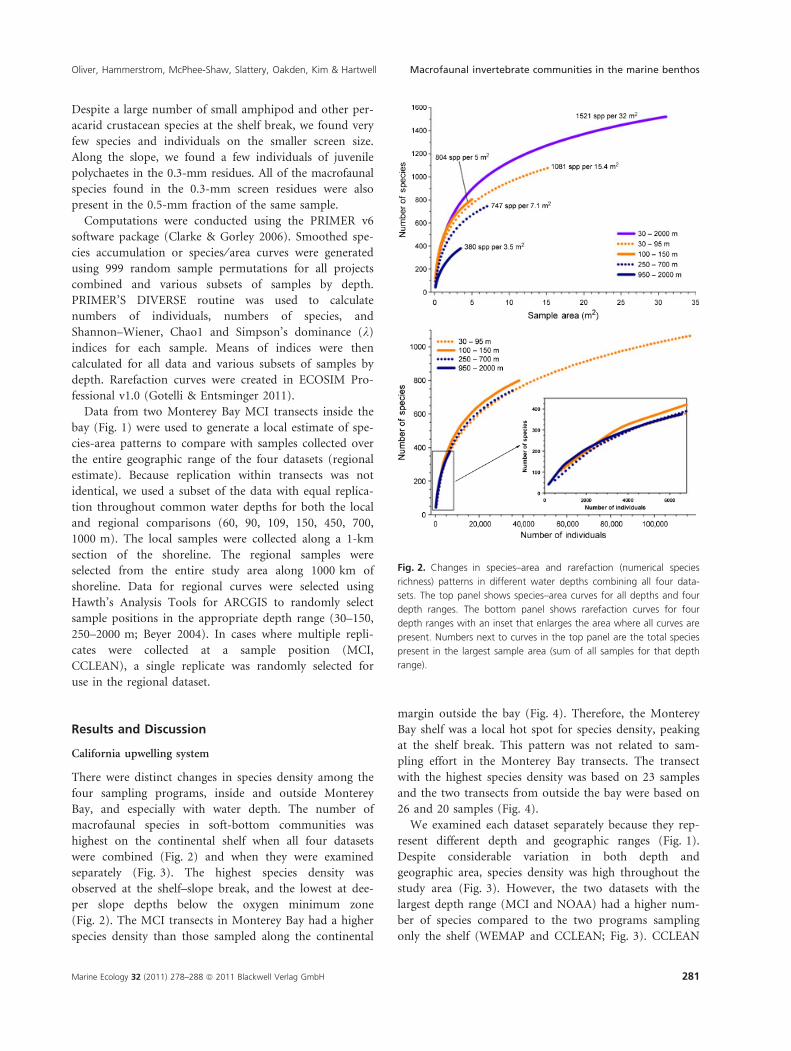
Fig. 2. Changes in species–area and rarefaction (numerical species
richness) patterns in different water depths combining all four data-
sets. The top panel shows species–area curves for all depths and four
depth ranges. The bottom panel shows rarefaction curves for four
depth ranges with an inset that enlarges the area where all curves are
present. Numbers next to curves in the top panel are the total species
present in the largest sample area (sum of all samples for that depth
range).
Oliver, Hammerstrom, McPhee-Shaw, Slattery, Oakden, Kim & Hartwell Macrofaunal invertebrate communities in the marine benthos
Marine Ecology 32 (2011) 278–288 ª 2011 Blackwell Verlag GmbH 281
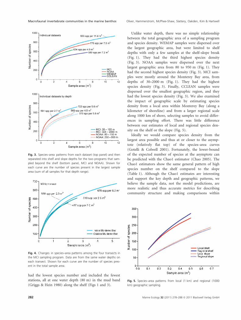
had the lowest species number and included the fewest
stations, all at one water depth (80 m) in the mud band
(Griggs & Hein 1980) along the shelf (Figs 1 and 3).
Unlike water depth, there was no simple relationship
between the total geographic area of a sampling program
and species density. WEMAP samples were dispersed over
the largest geographic area, but were limited to shelf
depths with only a few samples at the shelf–slope break
(Fig. 1). They had the third highest species density
(Fig. 3). NOAA samples were dispersed over the next
largest geographic area from 80 to 950 m (Fig. 1). They
had the second highest species density (Fig. 3). MCI sam-
ples were mostly around the Monterey Bay area, from
depths of 30–2000 m (Fig. 1). They had the highest
species density (Fig. 3). Finally, CCLEAN samples were
dispersed over the smallest geographic region, and they
had the lowest species density (Fig. 3). We also examined
the impact of geographic scale by estimating species
density from a local area within Monterey Bay (along a
kilometer of shoreline) and from a larger regional scale
along 1000 km of shore, selecting samples to avoid differ-
ences in sampling effort. There was little difference
between our estimates of local and regional species den-
sity on the shelf or the slope (Fig. 5).
Ideally we would compare species density from the
largest area possible and thus at or closer to the asymp-
tote (relatively flat top) of the species–area curves
(Gotelli & Colwell 2001). Fortunately, the lower-bound
of the expected number of species at the asymptote can
be predicted with the Chao1 estimator (Chao 2005). The
Chao1 estimators show the same general pattern of high
species number on the shelf compared to the slope
(Table 1). Although the Chao1 estimates are interesting
and support the key depth and geographic patterns, we
believe the sample data, not the model predictions, are
more realistic and thus accurate metrics for describing
community structure and making comparisons within
Fig. 3. Species–area patterns from each dataset (top panel) and then
separated into shelf and slope depths for the two programs that sam-
pled beyond the shelf (bottom panel, MCI and NOAA). Shown for
each curve are the number of species present in the largest sample
area (sum of all samples for that depth range).
Fig. 4. Changes in species–area patterns among the four transects in
the MCI sampling program. Data are from the same water depths on
each transect. Shown for each curve are the number of species pres-
ent in the total sample area.
Fig. 5. Species–area patterns from local (1 km) and regional (1000
km) geographic sampling.
Macrofaunal invertebrate communities in the marine benthos Oliver, Hammerstrom, McPhee-Shaw, Slattery, Oakden, Kim & Hartwell
282 Marine Ecology 32 (2011) 278–288 ª 2011 Blackwell Verlag GmbH
and between communities. The species–area curves
crossed only at the smallest sample areas, where there
was the greatest variability between single samples. Once
samples were combined, the variability was reduced at
larger sample areas and the relative differences among
the curves persisted to the end of each curve (e.g. Fig. 3
top panel).
The presence of an oxygen minimum zone (OMZ) did
not account for the lower species density on the slope
compared to the shelf. The OMZ is between 500 and
1000 m in the study area (Mullins et al. 1985; Johnson
et al. 1992). Although oxygen levels in the Central Cali-
fornia coastline’s OMZ are relatively low compared to
some upwelling regions (Levin 2003), the center of the
OMZ harbored a dense community of ampeliscid amphi-
pods, forming a tube mat that was seen in ROV video
footage along all four of the MCI depth transects (Fig. 1).
We sampled in the tube mat from the center of the OMZ
at 700 m and included these samples in the upper slope,
where there was relatively high species density (Fig. 2).
The lowest species densities were found below the OMZ
at 1000–2000 m (Fig. 2).
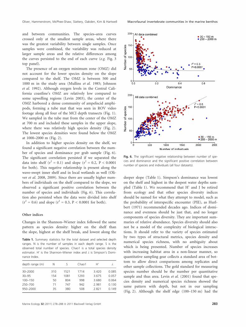
In addition to higher species density on the shelf, we
found a significant negative correlation between the num-
ber of species and dominance per grab sample (Fig. 6).
The significant correlation persisted if we separated the
data into shelf (r2 = 0.1) and slope (r2 = 0.2, P < 0.0001
for both). This negative relationship is present along the
wave-swept inner shelf and in local wetlands as well (Oli-
ver et al. 2008, 2009). Since there are usually higher num-
bers of individuals on the shelf compared to the slope, we
observed a significant positive correlation between the
number of species and individuals (Fig. 6). This correla-
tion also persisted when the data were divided into shelf
(r2 = 0.6) and slope (r2 = 0.3, P < 0.0001 for both).
Other indices
Changes in the Shannon–Wiener index followed the same
pattern as species density: higher on the shelf than
the slope, highest at the shelf break, and lowest along the
deeper slope (Table 1). Simpson’s dominance was lowest
on the shelf and highest in the deepest water depths sam-
pled (Table 1). We recommend that H’ and J be retired
from ecology and that other species diversity indices
should be named for what they attempt to model, such as
the probability of interspecific encounter (PIE), as Hurl-
bert (1971) recommended decades ago. Indices of domi-
nance and evenness should be just that, and no longer
components of species diversity. They are important sum-
maries of relative abundance. Species diversity should also
not be a model of the complexity of biological interac-
tions. It should refer to the variety of species estimated
by two types of structural metrics, species density and
numerical species richness, with no ambiguity about
which is being presented. Number of species increases
with increasing habitat area in a non-linear manner, so
quantitative sampling gear collects a standard area of bot-
tom to allow direct comparisons among replicates and
other sample collections. The gold standard for measuring
species number should be the number per quantitative
sample and thus area. Levin et al. (2001) found that spe-
cies density and numerical species richness showed the
same pattern with depth, but not in our sampling
(Fig. 2). Although the shelf edge (100–150 m) had the
Fig. 6. The significant negative relationship between number of spe-
cies and dominance and the significant positive correlation between
number of species and individuals (all four datasets).
Table 1. Summary statistics for the total dataset and selected depth
ranges. N is the number of samples in each depth range. S is the
observed total number of species. Chao1 is a total species density
estimator. H’ is the Shannon–Wiener index and k is Simpson’s Domi-
nance Index.
depth range (m) N S Chao1 H’ k
30–2000 310 1521 1714 3.420 0.085
30–95 154 1081 1293 3.675 0.057
100–150 50 804 998 3.680 0.064
250–700 71 747 942 2.981 0.130
950–2000 35 380 508 2.821 0.149
Oliver, Hammerstrom, McPhee-Shaw, Slattery, Oakden, Kim & Hartwell Macrofaunal invertebrate communities in the marine benthos
Marine Ecology 32 (2011) 278–288 ª 2011 Blackwell Verlag GmbH 283

highest numerical species richness and species density,
numerical richness at the other depths were quite similar
(Fig. 2). Therefore, we cannot always expect numerical
species richness and species density to show the same
depth and geographic patterns.
Numerical species richness often peaks along the slope
(Rex 1981, 1983; Levin et al. 2001), but not always
(Menot et al. 2010). Species density in the deep-sea may
also be high along the slope, but there are high values
from the shelf as well (Table 2). Although we did not
observe high species density from the slope depths we
sampled (Figs 2 and 3), there are high values along the
slope outside San Francisco Bay (Table 2), which is only
100 km north of Monterey Bay (Fig. 1). The important
similarity in all these data is that the highest values
(species density and numerical species richness) are
along the continental margins (Table 2, Menot et al.
2010). The species density data clearly show that slope
and shelf communities both have extremely high values
(Table 2).
If we could shrink ourselves and walk through the
benthic community as we can walk through a forest, the
number of species would clearly be higher on the shelf
than on the slope (Figs 2 and 3). If we walked from the
scale of a sample (0.1-m2) to the local setting and
through the regional geography, the variety of species
would be higher on the shelf at all spatial scales
(Figs 2–5). This is not reflected in numerical species
richness, which showed little difference between the shelf
and slope (Fig. 2). We would also encounter a much
greater number of individuals and less dominance on
the shelf (Fig. 6, Table 1). A higher species density
(Fig. 2), larger number of animals (Fig. 6), and greater
evenness of relative abundance (Fig. 6) would lead
most naturalists to conclude that the complexity of
biological interactions should be higher on the shelf (all
other things being equal for the walk). There is no
model (probability of interspecific encounter or
other) that combines these fundamental community
metrics into a single metric of community complexity
(structure or function) without obscuring the most
important ecological realities observed during our
hypothetical walk. Numerical species richness is a fine
addition to the three metrics and is especially useful if
we do not have samples of a standard area. If quantita-
tive samples are taken, species density should be
measured and presented in species–area curves for
community descriptions. Despite the statistical inconve-
nience of the correlation between the number of species
and individuals (Fig. 6), the most realistic community
description is done in a known spatial context, especially
for comparisons among samples, community patches,
and different communities.Tab
le2.
Com
par
ison
of
spec
ies
den
sity
of
soft
-bott
om
mac
roben
thos
from
the
upw
ellin
gco
ast
of
Cal
iforn
iaan
doth
erso
ft-b
ott
om
com
munitie
sw
ith
hig
hsp
ecie
sden
sity
.
sam
ple
area
(m2)
Cen
tral
Cal
iforn
iaco
ntinen
talsh
elf
and
slope
spec
ies
den
sity
spec
ies
den
sity
inw
orldw
ide
studie
s
30–1
50
alldat
a
250–2
000
alldat
a
30–1
50
MC
I&
NO
AA
30–1
50
MC
I
80–1
50
NO
AA
33–1
23
WEM
AP
80
CC
LEA
N
no.
of
spec
ies
dep
th(m
)
siev
esi
ze
(mm
)lo
cation
23.1
01286
a886
90–5
65
0.3
0Sa
nta
Mar
ia,
CA
,U
SA1
21.0
01286
a798
1500–2
500
0.3
0N
J&
DE,
USA
2
17.1
91231
b952
250–2
180
0.3
0G
eorg
esBan
k,U
SA3
13.5
01153
858
c1202
600–3
500
0.3
0C
arolin
aSl
ope,
USA
(SA
CSA
R)4
13.5
01153
858
c810
2160–3
142
0.3
0Sa
nFr
anci
sco,
CA
,U
SA5
13.3
01148
858
c1295
600–3
500
0.3
0C
arolin
aSl
ope,
USA
(SA
CSA
R)6
10.4
01069
853
957
d803
11–5
11.0
0Bas
sSt
rait,
Aust
ralia
7
5.6
7937
g706
g858
g723
e634
f549
599
1220–1
350
0.3
0N
ewEn
gla
nd,
USA
(NA
CSA
R)3
2.5
0652
512
653
568
549
531
447
511*
400–1
800
0.4
2H
ebrides
Slope,
Scotlan
d,
UK
8
1.2
5487
364
493
440
436
405
362
314
1230
0.4
2Sa
nD
iego
Trough,
CA
,U
SA9
0.8
1418
h301
h401
h364
h366
h337
h310
h436
800
0.3
0C
har
lest
on,
SC,
USA
4
0.6
8363
253
371
335
343
314
292
250
3600
0.3
0N
ewEn
gla
nd,
USA
10
Tota
lsa
mple
area
(m2)
=a20.4
,b17.2
,c 1
0.6
,d8.3
,e5.6
,f 4
.9,g
5.7
,h0.8
0;
*Pe
raca
rid
crust
acea
ns
not
iden
tified
.1H
ylan
det
al.
(1991);
2G
rass
le&
Mac
iole
k(1
992);
3C
ited
inLe
vin
etal
.(2
001);
4Bla
ke&
Gra
ssle
(1994);
5Bla
keet
al.
(2009);
6H
ilbig
(1994);
7G
ray
etal
.(1
997);
8G
age
etal
.(2
000);
9Ju
mar
s
(1976);
10G
rass
le&
Mors
e-Po
rteo
us
(1987).
Macrofaunal invertebrate communities in the marine benthos Oliver, Hammerstrom, McPhee-Shaw, Slattery, Oakden, Kim & Hartwell
284 Marine Ecology 32 (2011) 278–288 ª 2011 Blackwell Verlag GmbH

Worldwide patterns
We compared our data with the highest species densities
in soft sediments that we could find in the literature
(Table 2). Species density from the continental shelf in
Monterey Bay was very similar to levels reported from
the Carolina slope, which has the highest species densities
in the world reported to date, with a peak at 800 m
(436 ⁄ 0.81 m2; Table 2). The Carolina slope has a hetero-
geneous bottom with dynamic currents and likely high
inputs of food (Blake & Grassle 1994). The second high-
est species density from the shelf was documented on the
Australian side of Bass Strait between Australia and Tas-
mania (Gray et al. 1997). The species density was also
high on the shelf and highest at the shelf break at the
southern end of the California upwelling system (Hyland
et al. 1991). It appears that the soft-bottom shelf commu-
nities with the highest species densities in the world were
found in well-mixed and oxygenated waters with high
production (Breaker & Broenkow 1994; Pennington &
Chavez 2000; Fitzwater et al. 2003; McGinley 2008; Ryan
et al. 2009). These general habitat characteristics are simi-
lar to the current-dominated Carolina slope with the
highest species densities in the world (Blake & Grassle
1994).
Escaravage et al. (2009) documented a positive rela-
tionship between species density and productivity in soft
bottoms from a compiled dataset covering the European
coast (primarily from the shelf). They include two studies
with moderately high species density: the highest with
1033 species in 34.4 m2 from the Aegean. We found 1531
in 32 m2 (Fig. 1). There are 952 in 17.19 m2 along the
Georgia Banks (Table 2), which is half the sample area
from the Aegean. Table 2 does not include a number of
other studies with moderately high species density (e.g.
Gage 1979; Gray et al. 1997; Stora et al. 1999; Thiel et al.
2007; Dahle et al. 2009).
Differences between sampling methods and sample
dispersion do not confound comparisons between our
data and those from other parts of the world (Table 2).
All the data in Table 2 come from quantitative samples.
We are not comparing species density to numerical spe-
cies richness (Abele & Walters 1979; Gray et al. 1997).
The differences in screen size do not lead to unrealistic
comparisons, but some must be qualified, especially the
samples from Bass Strait. We found no loss of species
between the 0.5- and 0.3-mm screens, so our data can
be compared to samples that were washed through the
smaller screen (most of the data in Table 2). Samples
from two of the slope sites were washed through 0.42-
mm screens, potentially losing some species that could
be captured on a 0.3-mm mesh. The samples from Scot-
land do not include the peracarid crustaceans, so species
density should be even higher here. We include the two
0.42-mm surveys because they found high species density
despite their use of a larger sieve mesh size. Bass Strait
samples were dispersed over a small geographic area and
depth range and washed over a 1-mm screen, which
could significantly depress species density. Despite these
likely losses, Bass Strait has a high species density
(Table 2, Gray et al. 1997). If the sampling included the
entire shelf and a 0.5-mm screen, species density might
be more similar to that in Monterey Bay and along the
Carolina slope. Although there are considerable differ-
ences in the depth and geographic ranges of the data
from other parts of the world, many of these differences
are similar to the variation in our study, which includes
samples from one depth, two depth zones on the shelf
and slope, the shelf and slope combined, and several dif-
ferent geographic scales with different depth ranges.
None of the differences discussed above invalidates the
comparisons in Table 2.
Boundary effects
All of the communities with the highest species densities
(Table 2) are located along continental margins, where
there are dramatic changes in topography. The continental
slope is probably the most extensive steep rise in topogra-
phy in the ocean. The shelf–slope break is the most
abrupt topographic change along the slope. Pelagic pri-
mary productivity at the ocean surface is often highest
over the continental shelf and drops rapidly at the shelf
break and over the slope (Kudela et al. 2008). However,
we found a strikingly different pattern in benthic species
density. The highest species density in our study occurred
around the shelf–slope break (Fig. 2). We documented
804 species in 5 m2 (Fig. 2, top panel) collected from 100
to 150 m. Four of the locations from other parts of the
world reported about 800 species, but they were collected
in sample areas that were two to four times larger than
5 m2 (Table 2).
What is it about the shelf break that might cause such
high species densities? Although the continental shelf is
often characterized by an accumulation of fine material (a
‘shelf mud belt’), the outer shelf and upper slope usually
comprise coarser grained sediments, a relict from glacial
low sea stands. Oceanographers have long discussed the
reasons that the relatively abrupt change in topographic
steepness at the shelf break might enhance currents and
frictional dissipation of long-wavelength features such as
tides and low-mode internal tides (Sverdrup et al. 1942).
Abrupt topographic changes such as those found on
Georges Banks or on the European shelf seas can cause
tidal mixing fronts and intense, rapid exchange between
the sea floor and near-surface waters (Houghton &
Oliver, Hammerstrom, McPhee-Shaw, Slattery, Oakden, Kim & Hartwell Macrofaunal invertebrate communities in the marine benthos
Marine Ecology 32 (2011) 278–288 ª 2011 Blackwell Verlag GmbH 285

Ho 2001), and a seasonal shelf-break front is a common
feature of the Northeastern Atlantic (Chapman & Lentz
1994). Although such features are not typically found
over the continental shelves of California, they still serve
to illustrate the sometimes dramatic changes in dynamics
and energy near the shelf–slope break (see review,
McPhee-Shaw 2006). Studies from the California margin
demonstrate that interaction between internal tides and
topography intensify cross-isobath currents over the
upper continental slope and are associated with removal
of fine sediments from the margin (Cacchione et al. 2002;
McPhee-Shaw et al. 2004).
These variations in energy and dynamics can have an
array of effects on benthic habitat. Intense up-slope and
down-slope excursions associated with internal tides
expose benthic organisms, which are fixed in space, to
several hundred meters of vertical water column gradients
of temperature and oxygen, and over brief time scales
(<12 h). These water movements may also bring more
food to the benthos. Energetic currents prevent the accu-
mulation of fine material, and presumably allow greater
penetration of oxygen and nutrients into the substrate.
Thus, just as in freshwater ecosystems, where the well
mixed and oxygenated gravel and mixed-substrate under
medium-to-energetic streams have a much higher density
of macroinvertebrates than the substrates under either
very strong rivers or under the still waters of deep chan-
nels, ponds, and lakes (Karr & Chu 1999), the shelf–slope
break and upper slope may be an ideal habitat for ocean
benthic communities. Although more diffuse in space and
larger in scale, the shelf break and upper continental slope
may be analogous to the species-rich hard-bottom com-
munities of coral reefs and ocean pinnacles, both of
which have a topography that enhances water motion
and the transport of food and nutrients to the sea floor
(Genin et al. 1986; Koslow 1997; Leichter et al. 1998;
Genin 2004).
Summary
1 We found 1521 species of macrofaunal invertebrates in
32 m2 of bottom from the California upwelling system
(Fig. 2), where soft-bottom species density is among the
highest in the world (Table 2).
2 Species density was consistently higher along the shelf
(30–150 m) than along the slope (250–2000 m; Figs 2
and 3), with the highest number of species at the shelf–
slope break (Fig. 2: 100–150 m) coincident with breaking
internal waves and in the Monterey Bay under an upwell-
ing plume and production hot spot (Fig. 4).
3 Numerical species richness did not show the same
depth pattern as species density, which we consider the
best local and regional estimate of species number.
4 There was a significant negative correlation between
the number of species and dominance.
5 Species density from the California shelf is remarkably
similar to that reported from the Carolina slope, at both
local (800 m compared to the shelf break) and regional
scales (Table 2). Species density at these two sites is con-
siderably higher than anywhere else in the world.
Acknowledgements
Paul Dayton is a great example as a scientist and friend. He
taught us the paramount importance of natural history,
time series, human disruptions, laughing, and good pies.
We owe thanks to Lisa Levin, Jim Blake and the anony-
mous reviewers, Coastal Conservation and Research Inc.
for producing the WEMAP data, ABA Consultants for pro-
viding the CCLEAN and MCI data, Rusty Fairey and Ivano
Aiello at Moss Landing Marine Labs, and Steve Weisberg
and Ananda Ranasinghe of the Southern California Coastal
Water Research Project. We are most grateful to the many
invertebrate taxonomists who make our estimates of com-
munity structure possible: Kelvin Barwick (Mollusca), Don
Cadien (Crustacea), Hank Chaney (Gastropoda), Matt For-
rest (Ectoprocta), Leslie Harris (Polychaeta), Gordon Hen-
dler (Ophiuroidea), Mike Kellogg (Mollusca), Louis
Kornicker (Ostracoda), Linda Kuhnz (Mollusca), Gretchen
Lambert (Ascidacea), Welton Lee (Porifera), Megan Lilly
(Ophiuroidea), John Ljubenkov (Cnidaria), Josh Mackie
(Oligochaeta), Tony Phillips (Nemertea), Gene Ruff (Poly-
chaeta), Paul Valentich-Scott (Mollusca). We would also
like to thank the many students and staff who assisted in
fieldwork, sample processing, and sorting.
References
ABA Consultants (2000) MCI ⁄ Worldcom Southern Cross
Monterey Bay Cable Landing, Technical Memorandum 5.
Offshore Studies: Physical Oceanography and Marine
Biology. Prepared for Natural Resources Consultants, CA,
207 pp.
Abele L.G., Walters K. (1979) Marine benthic diversity: a cri-
tique and alternative explanation. Journal of Biogeography, 6,
115–126.
Beyer H.L. (2004) Hawth’s Analysis Tools for ArcGIS. http://
www.spatialecology.com/htools.
Blake J.A., Grassle J.F. (1994) Benthic community structure on
the US South Atlantic slope off the Carolinas: spatial hetero-
geneity in a current-dominated system. Deep-Sea Research
Part II, 41, 835–874.
Blake J.A., Maciolek N.J., Ota A.Y., Williams I.P. (2009) Long-
term benthic infaunal monitoring at a deep-ocean dredged
material disposal site off Northern California. Deep-Sea
Research Part II, 56, 1775–1803.
Macrofaunal invertebrate communities in the marine benthos Oliver, Hammerstrom, McPhee-Shaw, Slattery, Oakden, Kim & Hartwell
286 Marine Ecology 32 (2011) 278–288 ª 2011 Blackwell Verlag GmbH

Breaker L.C., Broenkow W.W. (1994) The circulation of Mon-
terey Bay and related processes. Oceanography and Marine
Biology: An Annual Review, 32, 1–64.
Cacchione D.A., Pratson L.F., Ogston A.S. (2002) The shaping
of continental slopes by internal tides. Science, 296, 724–727.
Chao A. (2005) Species estimation and applications. In: Bala-
krishnan N., Read C.B., Vidakovic B. (Eds), Encyclopedia of
Statistical Sciences, 2nd edn. 12, 7907–7916. Wiley, New
York.
Chapman D.C., Lentz S.J. (1994) Trapping of a coastal density
front by the bottom boundary layer. Journal of Physical
Oceanography, 24, 1464–1479.
Clarke K.R., Gorley R.N. (2006) PRIMER v6: User Manual ⁄Tutorial. PRIMER-E, Plymouth.
Dahle S., Anisimova N.A., Palerud R., Renaud P.E., Pearson
T.H., Matishov G.G. (2009) Macrobenthic fauna of the
Franz Josef Land archipelago. Polar Biology, 32, 169–180.
Dayton P.K., Hessler R.R. (1972) Role of biological distur-
bance in maintaining diversity in the deep sea. Deep-Sea
Research, 19, 199–208.
Escaravage V., Herman P.M.J., Merckx B., Wlodarska-Kow-
alczuk M., Amouroux J.M., Degraer S., Gremare A., Heip
C.H.R., Hummel H., Karakassis I., Labrune C., Willems W.
(2009) Distribution patterns of macrofaunal species diversity
in subtidal soft sediments: biodiversity-productivity relation-
ships from the MacroBen database. Marine Ecology Progress
Series, 382, 253–264.
Fitzwater S.E., Johnson K.S., Elrod V.A., Ryan J.P., Coletti L.J.,
Tanner S.J., Gordon R.M., Chavez F.P. (2003) Iron, nutrient
and phytoplankton biomass relationships in upwelled waters
of the California coastal system. Continental Shelf Research,
23, 1523–1544.
Gage J.D. (1979) Macrobenthic community structure in the
Rockall Trough. Ambio Special Report, 6, 43–46.
Gage J.D., Lamont P.A., Kroeger K., Paterson G.L.J., Gonzalez
Vecino J.L. (2000) Patterns in deep-sea macrobenthos at the
continental margin: standing crop, diversity, and faunal
change on the continental slope off Scotland. Hydrobiologia,
440, 261–271.
Genin A. (2004) Bio-physical coupling in the formation of
zooplankton and fish aggregations over abrupt topographies.
Journal of Marine Systems, 50, 3–20.
Genin A., Dayton P.K., Lonsdale P.F., Spiess F.N. (1986)
Corals on seamount peaks provide evidence of
current acceleration over deep-sea topography. Nature, 322,
59–61.
Goodman D. (1975) The theory of diversity-stability relation-
ships in ecology. Quarterly Review of Biology, 50, 237–266.
Gotelli N.J., Colwell R.K. (2001) Quantifying biodiversity: pro-
cedures and pitfalls in the measurement and comparison of
species richness. Ecology Letters, 4, 379–391.
Gotelli N.J., Entsminger G.L. (2011) EcoSim Professional: Null
Modeling Software For Ecologists. Version 1.0. Acquired Intel-
ligence Inc., Kesey-Bear & Pinyon Publishing, Jerico, VT,
USA. http://www.garyentsminger.com/ecosim/index.htm.
Grassle J.F., Maciolek N.J. (1992) Deep-sea species richness:
regional and local diversity estimates from quantitative
bottom samples. American Naturalist, 139, 313–341.
Grassle J.F., Morse-Porteous L.S. (1987) Macrofaunal coloniza-
tion of disturbed deep-sea environments and the structure
of deep-sea benthic communities. Deep-Sea Research Part II,
34, 1911–1950.
Gray J.S., Poore G.C.B., Ugland K.I., Wilson R.S., Olsgard F.,
Johannessen Ø. (1997) Coastal and deep-sea benthic diversi-
ties compared. Marine Ecology Progress Series, 159, 97–103.
Griggs G.B., Hein J.R. (1980) Sources, dispersal, and clay min-
eral composition of fine-grained sediments off central and
northern California. Journal of Geology, 88, 541–566.
Hilbig B. (1994) Faunistic and zoogeographical characteriza-
tion of the benthic infauna on the Carolina continental
slope. Deep-Sea Research Part II, 41, 929–950.
Houghton R.W., Ho C. (2001) Diapycnal flow through the
Georges Bank tidal front: a dye tracer study. Geophysical
Research Letters, 28, 33–36.
Hurlbert S.H. (1971) The nonconcept of species diversity: a
critique and alternative parameters. Ecology, 52, 577–586.
Hyland J., Baptiste E., Campbell J., Kennedy J., Kropp R.,
Williams S. (1991) Macroinfaunal communities of the Santa
Maria Basin on the California outer continental shelf and
slope. Marine Ecology Progress Series, 78, 147–161.
Johnson K.S., Berelson W.M., Coale K.H., Coley T.L., Elrod
V.A., Fairey W.R., Iams H.D., Kilgore T.E., Nowicki J.L.
(1992) Manganese flux from continental margin sediments
in a transect through the oxygen minimum. Science, 257,
1242–1245.
Jumars P.A. (1976) Deep-sea species diversity: does it have
a characteristic scale? Journal of Marine Research, 34, 217–
246.
Karr J.R., Chu E.W. (1999) Restoring Life in Running Waters:
Better Biological Monitoring. Island Press, Washington, DC:
206 pp.
Koslow J.A. (1997) Seamounts and the ecology of deep-sea
fisheries. American Scientist, 85, 168–176.
Kudela R.M., Banas N.S., Barth J.A., Frame E.R., Jay D.,
Largier J.L., Lessard E.J., Peterson T.D., Vander Woude A.J.
(2008) New insights into the controls and mechanisms of
plankton productivity along the US West Coast. Ocean-
ography, 21, 46–59.
Leichter J.J., Shellenbarger G., Genovese S.J., Wing S.R. (1998)
Breaking internal waves on a Florida (USA) coral reef: a
plankton pump at work? Marine Ecology Progress Series, 166,
83–97.
Levin L.A. (2003) Oxygen minimum zone benthos: adaptation
and community response to hypoxia. Oceanography and
Marine Biology: an Annual Review, 41, 1–45.
Levin L.A., Etter R.J., Rex M.A., Gooday A.J., Smith C.R.,
Pineda J., Stuart C.T., Hessler R.R., Pawson D. (2001)
Environmental influences on regional deep-sea species
diversity. Annual Review of Ecology and Systematics, 32,
51–93.
Oliver, Hammerstrom, McPhee-Shaw, Slattery, Oakden, Kim & Hartwell Macrofaunal invertebrate communities in the marine benthos
Marine Ecology 32 (2011) 278–288 ª 2011 Blackwell Verlag GmbH 287

McGinley M. (2008) Southeast Australian Shelf large marine
ecosystem. In: Cleveland C.J. (Ed), Encyclopedia of Earth.
Environmental Information Coalition, National Council for
Science and the Environment, Washington, DC: http://
www.eoearth.org/article/Southeast_Australian_Shelf_large_
marine_ecosystem.
McPhee-Shaw E.E. (2006) Boundary–interior exchange: review-
ing the idea that internal-wave mixing enhances lateral dis-
persal near continental margins. Deep-Sea Research Part II,
53, 42–59.
McPhee-Shaw E.E., Sternberg R.W., Mullenbach B., Ogston
A.S. (2004) Observations of intermediate nepheloid layers
on the northern California margin. Continental Shelf
Research, 24, 693–720.
Menot L., Sibuet M., Carney R.S., Levin L.A., Rowe G.T., Bil-
lett D.S.M., Poore G., Kitazato H., Vanreusel A., Galeron J.,
Lavrado H.P., Sellanes J., Ingole B., Krylova E. (2010) New
perceptions of continental margin biodiversity. In: McIntyre
A.D. (Ed), Life in the World’s Oceans: Diversity, Distribution,
and Abundance. Wiley-Blackwell, UK: 79–101.
Mullins H.T., Thompson J.B., McDougall K., Vercoutere T.L.
(1985) Oxygen-minimum zone edge effects: evidence from
the central California coastal upwelling system. Geology, 13,
491–494.
Oliver J.S., Slattery P.N., Hulberg L.W., Nybakken J.W. (1980)
Relationships between wave disturbance and zonation of
benthic invertebrate communities along a high-energy sub-
tidal beach in Monterey Bay, California. Fishery Bulletin, 78,
437–454.
Oliver J.S., Kim S.L., Slattery P.N., Oakden J.M., Hammer-
strom K.K., Barnes E.M. (2008) Sandy bottom communities
at the end of a cold (1971–1975) and warm regime (1997–
1998) in the California Current: impacts of high and low
plankton production. Available from Nature Precedings.
<http://dx.doi.org/10.1038/npre.2008.2103.1>.
Oliver J.S., Hammerstrom K.K., Aiello I.W., Oakden J.M., Slat-
tery P.N., Kim S.L. (2009) Benthic invertebrate communities
in peripheral wetlands of Elkhorn Slough ranging from very
restricted to well-flushed by tides. Final report to Monterey
Bay National Marine Sanctuary and Elkhorn Slough
National Estuarine Research Reserve, CA, 77 pp.
Pennington J.T., Chavez F.P. (2000) Seasonal fluctuations of
temperature, salinity, nitrate, chlorophyll and primary
production at station H3 ⁄ M1 over 1989–1996 in Monterey
Bay, California. Deep-Sea Research Part II, 47, 947–973.
Rex M.A. (1981) Community structure in the deep-sea
benthos. Annual Review of Ecology and Systematics, 12, 331–
353.
Rex M.A. (1983) Geographic patterns of species diversity in
deep-sea benthos. In: Rowe G.T. (Ed.), The Sea, 8, 453–472.
Rex M.A., Stuart C.T., Coyne G. (2000) Latitudinal gradients
of species richness in the deep-sea benthos of the North
Atlantic. Proceedings of the National Academy of Sciences, 97,
4082–4085.
Ryan J.P., Fischer A.M., Kudela R.M., Gower J.F.R., King
S.A., Marin R., Chavez F.P. (2009) Influences of upwelling
and downwelling winds on red tide bloom dynamics in
Monterey Bay, California. Continental Shelf Research, 29,
785–795.
Sanders H.L. (1968) Marine benthic diversity: a comparative
study. American Naturalist, 102, 243–282.
Sanders H.L. (1969) Marine benthic diversity and the stability-
time hypothesis. In: Woodwell G.G., Smith H.H. (Eds),
Diversity and Stability in Ecological Systems. Brookhaven
Symposia in Biology, 22, 71–81.
Spellerberg I.F., Fedor P.J. (2003) A tribute to Claude Shannon
(1916–2001) and a plea for more rigorous use of species
richness, species diversity and the ‘Shannon-Wiener’ index.
Global Ecology & Biogeography, 12, 177–179.
Stora G., Bourcier M., Arnoux A., Gerino M., Le Campion J.,
Gilbert F., Durbec J.P. (1999) The deep-sea macrobenthos
on the continental slope of the northwestern Mediterranean
Sea: a quantitative approach. Deep-Sea Research Part I, 46,
1339–1368.
Sverdrup H., Johnson M.W., Fleming R.H. (1942) The Oceans
– their Physics, Chemistry, and General Biology. Prentice-Hall,
Englewood Cliffs, NJ.
Thiel M., Macaya E.C., Acuna E., Arntz W.E., Bastias H.,
Brokordt K., Camus P.A., Castilla J.C., Castro L.R., Cortes
M., Dumont C.P., Escribano R., Fernandez M., Gajardo
J.A., Gaymer C.F., Gomez I., Gonzalez A.E., Gonzalez H.E.,
Haye P.A., Illanes J., Iriarte J.L., Lancellotti D.A., Luna-Jor-
quera G., Luxoro C., Manriquez P.H., Marın V., Munoz P.,
Navarrete S.A., Perez E., Poulin E., Sellanes J., Sepulveda
H.H., Stotz W., Tala F., Thomas A., Vargas C.A., Vasquez
J.A., Alonso Vega J.M. (2007) The Humboldt Current
system of northern and central Chile. Oceanographic
processes, ecological interactions and socioeconomic feed-
back. Oceanography and Marine Biology: an Annual Review,
45, 195–345.
Macrofaunal invertebrate communities in the marine benthos Oliver, Hammerstrom, McPhee-Shaw, Slattery, Oakden, Kim & Hartwell
288 Marine Ecology 32 (2011) 278–288 ª 2011 Blackwell Verlag GmbH


