
DETERMINANTS OF EXCHANGE RATES: THE CASE OF THE CHILEAN PESO
Sebastian Zwanzger
A Thesis Submitted to the University of North Carolina Wilmington in Partial Fulfillment
of the Requirements for the Degree of Masters of Business Administration
Cameron School of Business
University of North Carolina Wilmington
2008
Approved by
Advisory Committee
Peter Schuhmann . Luther Lawson . .
. Cet Ciner . Chair
Accepted by
. . Dean, Graduate School

ii
TABLE OF CONTENTS
ABSTRACT ........................................................................................................................ iii
LIST OF TABLES ............................................................................................................... iv
LIST OF FIGURES .............................................................................................................. v
INTRODUCTION ................................................................................................................ 1
THEORIES BEHIND EXCHANGE RATE DETERMINATION, BRIEF REVIEW............. 3
BACKGROUND ON CHILE AND THE UNITED STATES – ECONOMY AND
CURRENCIES...................................................................................................................... 4
The U.S. Dollar ..................................................................................................................... 4
Exchange Rate Movements and Economic Performance........................................................ 4
Economic Background and exchange rate regime in Chile .................................................... 5
COMMODITY CURRENCIES ............................................................................................ 7
Chile and Copper .................................................................................................................. 9
DATA SOURCES AND COLLECTION METHODS......................................................... 10
Data Description ................................................................................................................. 10
Money Stock (M2) .............................................................................................................. 11
Monetary Policy Interest Rate ............................................................................................. 12
Data Split ............................................................................................................................ 12
EMPIRICAL ANALYSIS ................................................................................................... 13
Correlation Analysis............................................................................................................ 14
CONCLUSION................................................................................................................... 22
LITERATURE CITED ....................................................................................................... 24

iii
ABSTRACT
In this study, we analyzed the relationship between the exchange rate movements of
two countries, Chile and the United States, by studying the underlying fundamentals given by
the modern exchange rate theory. In this context, we included in our regression analysis three
main economic factors. Monetary policy interest rate, money supply and inflation rates were
considered for both countries since January 1990.
We also included a fourth variable in our model; Copper Price. The evolution of this
commodity’s price played an important role in our study as we will discover that a significant
portion in exchange rates variation is explained by this variable. Copper was considered
because of the increasing importance of this commodity in the Chilean economy.
The results show that the determinants of the exchange rate may vary over time. The
independent variables that have an effect on the exchange rate may lose their explanatory
power when economic conditions change or a switch in the foreign exchange rate policy
dictated by central banks or, as we proved, when variations on certain markets takes place.

iv
LIST OF TABLES
Table Page
1. Correlation Analysis................................................................................................. 14
2. Lagged Regression Coefficients ............................................................................... 21

v
LIST OF FIGURES
Figure Page
1. Evolution CHP/USD compared to the Chilean Inflation ............................................. 6
2. Evolution CHP/USD compared to the Evolution of Copper Price ............................... 9
3. CHP/USD – Inflation US and Chile – Copper Price Evolution ................................. 12
INTRODUCTION
Since the early seventies, several theories concerning exchange rates determination
have evolved. At this time, it was common to emphasize international trade flows as primary
determinants of exchange rates. This was due, in part, to the fact that governments
maintained tight restrictions on international flows of financial capital. The role of exchange
rate changes in eliminating international trade imbalance suggest that we would expect
countries with current trade surpluses to have an appreciating currency, whereas countries
with trade deficits should have depreciating currencies.
These different models developed mainly in the 70’s led to testable propositions in
which the changes in the exchange rate are linearly related to the news in the fundamental
variables, such as money stocks, prices, output, current accounts, etc. Among these models,
we find the monetary model, Dornbush model, and the portfolio balance model.
We can consider this as the first stage in exchange rate determination theory.
Unfortunately, these first generation models were rejected by the data, at least for countries
where the levels of inflation where relatively low. Three anomalies were detected.
• First, the random walk forecast typically outperforms a forecast based on the first
generation models. The study conducted by Meese and Regoff (1983 – 1988)
demonstrated that the theory behind these models can’t be confirmed by the results of
the study. Random walk theory states that currencies take a random and unpredictable
path.
• Second, since the start of the floating exchange rate regime, variability of exchange
rates increased dramatically. At the same time, there is no evidence to be found that
the variability of the fundamentals identified by the theoretical models has increased
compared to the fix exchange rates period. First generation models implied that the
variability of exchange rates can only increase when the variability of the underlying
fundamentals increases
• Third, the first stage models assume that exchange rates can only change at a certain
point in time as a result of “news” in the fundamentals. A study directed by De Boeck
(2000) and Altavilla (2000) find that unanticipated shocks in the fundamental
variables explain only a small fraction of the unanticipated changes in exchange rates.

2
Typically they find that news on inflation, output and interest rates explain about 5%
in the variation of exchange rates.
At this point, where theory has been proven wrong, researchers are driven to alternatives
to this first stage models. Some studies introduce nonlinearities into the model (see De
Grauwe and Dewatcher, 1993; Frankel and Frot, 1990; Kilian and Taylor, 2003; Kurz and
Motolese, 1999). These models are characterized by the existence of several agents using
different information sets and/or by the existence of transaction costs. The insight provided
by these models is that they predict frequent structural breaks in linear exchange rate
equations, and that they allow for changes in the exchange rates that are unrelated to news
about the underlying fundamentals.
It is also worth mentioning and considering the contribution of Nelson C. Mark (1995)
where he investigates the extent to which deviations of the exchange rate from a fundamental
value suggested by economic theory are useful in predicting exchange rates over long
horizons. The study presents evidence that there is an economically significant component in
long horizon changes in log nominal exchange rates. This was made by testing regressions of
multipleperiod changes in the log exchange rate on the deviation of the log exchange rate
from its “fundamental value”. The results of the study show that while short horizons changes
tend to be dominated by noise, this noise tend to be averaged out over time. The so called
“Noise” refers to exchange rates fluctuations in the market that can confuse one’s
interpretation of market direction. The study reveals systematic exchange rate movements
that are determined by economic fundamentals. This was one of the first studies that proved
with empirical results that exchange rate changes can be forecasted.
The objective of this project is, considering previous studies on the field, to analyze the
nature of the relationship between exchange rate changes and the variations in the underlying
fundamentals, looking at the historic development of two currencies, the US dollar and
Chilean Peso.
Besides testing the Chilean currency against the fundamental variables, a new test will be
performed taking into consideration the impact that commodity prices may have in foreign
exchange determination, in view of the high impact of copper in the Chilean economy.

3
THEORIES BEHIND EXCHANGE RATE DETERMINATION, BRIEF REVIEW
1. Purchasing Power Parity (PPP): Based on ‘no arbitrage argument’ or ‘law of one price’,
PPP is a flow model of the ‘inflation theory of exchange rates’ visavis the balance of
trade. Only relative PPP seems to hold in the long run. Shifts in technology, tastes,
commercial policies or labor force growth will structurally change national productivity
and hence will permanently change the real exchange rate.
2. Monetary Approach: These stock models are based on IS/LM/Phillip Curve paradigm.
Basically the theories are based on finding the exchange rate which the available amount
of currency supply is equal to the demand to hold the currency.
2.1 MundellFleming Model: The theory considers three markets: money, asset and goods
markets under perfect price flexibility in long run. One implication is devaluation may
lead to further devaluation if fiscal discipline, inflation and balance of payments are not
well managed. Another is that the higher the degree of reexport processing industry the
country has, the lower the impact of devaluation for current account improvement.
2.2 Monetarist Model: This concept implies that the exchange rate level is perfectly
correlated with the level of the relative money supply in long run. In a stationary
economy, the relative money growth rate would be zero and the exchange rate
expectation would play a trivial role. Postulated in an inflationary and/or high growth
economy, this model explains why a foreign exchange rate market may be
characterized by a selffulfilling prophecy. When the money supply becomes stochastic,
rational expectation and accuracy of market information play an important role in inter
temporal analysis.
2.3 ‘Sticky Price’ Model : When a currency is devalued and the price of goods remains
fixed in the short run, but not in the long run, the currency value may ‘overshoot’. A
balance of payment crisis, extended from the model, is the equilibrium outcome of
maximizing behavior by rational agents faced with a fundamental inconsistency
between monetary and exchange rate policies. One implication can be in a game
theoretic perspective in policy implementation. In a noncooperative and uncoordinated
game with many players, each individual player has little information on other players’
payoffs. There is no reason to believe everyone would act together to reach the desired
outcome in a single step. Good government coordination as a signal to the financial

4
market becomes essential to achieve effective monetary policy for currency
stabilization.
2.4. PortfolioBalance Approach: This theory determines the exchange rate as the relative
price of monies in short run. The asset substitution effects and the nature of
expectations formation places more emphasis on short run capital flows rather than the
trade balance. In general, the short run impact of policies can be quite different from the
long run impact, depending on the nature of the expectations. Exchange rates should
implicitly behave like the behavior of asset prices in speculative markets.
BACKGROUND ON CHILE AND THE UNITED STATES – ECONOMY AND
CURRENCIES
The U.S. Dollar
The US dollar accounts for about 70% of all foreignexchange reserves and over one
half of global private financial wealth. About twothirds of world trade is invoiced in US
dollars and threequarters of international bank lending is denominated in dollars. 1 The
dollars importance has, however, decreased since the mid1970s, when it was responsible for
80% of official reserves in foreign countries. Investors would start diversifying their
portfolios as the world moves towards a multiple currency system. A legitimate rival of the
USD is the Euro, especially after its introduction in 20002004, and in recent years many
countries have announced that they are increasing their euro reserves as it has an increasing
role in the world’s economy.
Exchange Rate Movements and Economic Performance
The 1990s was a period of unprecedented economic growth in the US, and in
February 2000 the economy surpassed the previous record for the longest sustained
expansion of 107 months. The main feature of the expansion was a steady improvement in
productivity, owing partly to wider use of computers and other advanced technology. Real
GDP grew by almost 40% between 1991 and 2001, equivalent to an annual average of 3.4%.
This economic prospect allowed the US dollar to appreciate throughout the nineties and
beginning of the new century against most trading partners. The Federal Reserve’s index of
1 www.eiu.com, country profile USA

5
the US dollar’s effective exchange rate against other major currencies rose from an average
of 94.06 in 1998 (March 1973=100) to 107.66 in 2001. The long appreciation of the dollar
reflected the strong underlying performance of the US economy and the prospect of high
investment returns.
The first indication that the long expansion was coming to an end came with the
collapse in the value of hightech stocks that began in March 2000. Investments slowed down
dramatically, while slow growth in the US.s major trading partners contributed to a
deteriorating trade balance. Growth slowed further during 2001, especially in the immediate
aftermath of the September 11th terrorist attacks. This was also a bad time for financial
markets, which were rocked by a number of major scandals. Most of these can be traced back
to the excesses of the stock market boom of the 1990s, when some highprofile companies
resorted to dubious accountancy practices to boost their profits and share prices.
Even as the US economy weakened and US interest rates fell during 2001, the US
dollar held its value against most currencies. Poor investments returns elsewhere in the world
contributed to the US dollar to maintain its value for that time.
However, the US dollar dropped in value significantly against most major currencies
during 2002, with the pace quickening in 200304, primarily against the euro and the Chinese
yen. This was also the case for the Chilean peso.
The central banks exchangerate index against major currencies averaged 93.o4 in
2003 and 85.42 in 2004, or nearly 21% below its 2001 average. 2 The depreciation reflected
concern about the widening currentaccount deficit and the rapid deterioration in the federal
government’s fiscal position. In 2005 the US dollar regained some strength, propelled by a
combination of rising shortterm interest rates in the US and the weakness of other
economies, notably those in the euro zone.
The US dollar reached a oneyear low of US $1.27 against the euro in May 2006, a
28year low of US$1.12 against the Canadian dollar, and also retreated significantly against
the yen. G7 finance ministers made it clear at a meeting in April 2006 that they would
welcome an appreciation of currencies of emerging economies with big trade surpluses with
the US, such as China and South Korea.
Economic Background and exchange rate regime in Chile
2 www.eiu.com, country profile USA

6
The Chilean peso trend had a remarkable inflexion point in the beginning of year
2003, where it reached its maximum value of 745.21 pesos per US dollar. The appreciation of
the CLP is evident after that date.
Starting in 1990, the Central Chilean Bank (CCB) adopted an inflation target regime.
An inflation objective was set every year and gradually adjusted so as to allow for an ongoing
reduction of inflation. In fact, in 1990, the target for the following year was set at 27%,
whereas in 2001 the target was 3%.
Figure 1. Evolution CHP/USD compared to the Chilean Inflation
From the mid eighties to September 7, 1999, the CCB adopted a crawling exchange
rate band, where the rate is allowed to fluctuate in a band around a central value, which is
adjusted periodically. The main objectives of the band were to maintain international
competitiveness and reduce excessive exchange rate volatility.
However, since the start of the band, many of its features, including its width, rate of
crawl, reference currency basket, degree of symmetry and central parity were modified. Since
September 2, 1999, the CCB has embraced a fully flexible exchange rate regime, with the

7
possibility of the CCB intervening in the market only in the case that “the exchange rate does
not reflect the real value of the foreign currency.”
However, the elimination of the band in September 1999 did not imply the absence of
foreign exchange interventions. In fact, in response to large exchange rate depreciation and
volatility, the CCB announced and carried out a temporary policy of sterilized interventions
between July 2001 and January 2002. The stated objectives of the interventions were to
reduce excessive exchange rate volatility and provide a hedge against future devaluations,
without affecting exchange rate trends.
COMMODITY CURRENCIES
Commodity currencies are those of countries which depend heavily on the export of
certain raw materials or commodities for income.
Different studies have been performed in this area to determine if such commodities
exporting countries see their currencies affected by variations on internationally traded
commodity prices. The study by YuChin Yen and Rogoff (2002) analyzed the relationship
between the exchange rate movements and commodity prices for Canada, New Zealand and
Australia. These countries were chosen because they constitute open economies and are
highly integrated to global capital markets and are dynamic participants in international trade.
All of them have been operating under a freely floating exchange rate regime. Commodity
exports account for 60% of Australia’s total exports and 50% for New Zealand. Canada has a
stronger industrial base, but still continues to rely more than a quarter of its exports on
commodities. The authors find that world prices of commodity exports, expressed in
American dollars, have a firm and stable influence on the exchange rates for Australia and
New Zealand. For Canada the influence is not as strong, but fairly significant. Even though
these countries have open capital markets and free floating exchange rate regimes, a real
explanatory variable was found for determining exchange rate movements.
Indeed, the study performed by Cashin, Céspedes, and Sahay (2002) based on the
assumption that fluctuations in real commodity prices have the potential to explain changes in
real exchange rates, given that many countries are highly dependent on commodities for their
exports revenues. They also studied the relationship between commodity prices and currency
determination, but expanded their study to all the commodities exporting countries. 58

8
commodity exporting countries were included in the sample. 53 of those are developing
countries 3 . “Commodity exports typically exceeded 50 percent of the total exports of several
subSaharan African countries, especially Burundi (97 percent), Madagascar (90 percent),
and Zambia (88 percent). The share of primary commodity exports in total exports was quite
high even for the industrial countries (Australia, 54 percent; Iceland, 56 percent).” 4
The results obtained by their study showed that 22 out of these 58 countries present a
surprisingly strong relationship that remains over time between commodity price shifts and
the currency determination. Half of these commoditycurrency countries belong to the sub
Saharan African countries, due to their strong dependence to commodities. In many cases
they rely on the exports of only one commodity. For these countries their commodities
exports usually account for more than 90% of their total exports. That is the case for
Dominica (bananas), Ethiopia (coffee), Mauritius (sugar), Niger (uranium), and Zambia
(copper).
Over 80% of the variation in the real exchange rate can, on average, be explained by
movements in real commodity prices alone. Measuring the impact of price variations, they
found that the elasticity typically ranged between 0.2 and 0.4, with a median of 0.38. Thus, a
10 percent drop in the real price of the commodity exports of countries with commodity
currencies is typically associated with a 3.8 percent depreciation of their real exchange rate.
Further analysis also indicated that, when deviations from the relationship between exchange
rates and commodity prices occurred in countries with commodity currencies, they were
caused primarily by changes in real commodity prices. Following a movement in commodity
prices, it is typically the real exchange rate that then adjusts to restore its longrun
relationship with real commodity prices. 5
3 (classified by the IMF's World Economic Outlook as exporters of nonfuel primary products and those with diversified export earnings) 4 Paul Cashin, Luis Céspedes, and Ratna Sahay (2002) 5 Paul Cashin, Luis Céspedes, and Ratna Sahay (2002)

9
Chile and Copper
Chile is the largest producer and exporter of copper in the world, followed by Peru,
USA and Indonesia. Utilized primarily in the construction industry, it is also widely used as a
conductor for electronic devises, house hold products, coinage, biomedical applications, and
chemical applications among others. Copper stands for 45% of Chilean exports and accounts
for 13.9% of Chile’s Nominal GDP. Chile produces 35.6% of the worlds copper production
and represents 30% of the world’s reserve of copper. 6
The study by Cashin, Céspedes, and Sahay (2002) does not consider Chile to be a
commodity currency country, but this may be explained because historic prices for copper
remained stable for the period studied. After 2003, copper prices started increasing at a very
quick pace due to growing world demand and a large drop in international inventories levels.
Our latter analysis is focused to determine if the relationship between copper price and
currency determination is stable and significant.
The following graph shows the evolution of CLP against the increase in price of a pound of
copper.
Figure 2. Evolution CHP/USD compared to the Evolution of Copper Price
Three commodity exchanges provide the facilities to trade copper: The London Metal
Exchange (LME), the Commodity Exchange Division of the New York Mercantile Exchange
(COMEX/NYMEX) and the Shanghai Metal Exchange (SHME). In these exchanges, prices
6 COCHILCO (Chilean Copper Commission)
0
50
100
150
200
250
300
350
400
450
0
100
200
300
400
500
600
700
800
dic‐85
ene‐87
ene‐88
ene‐89
ene‐90
ene‐91
ene‐92
ene‐93
ene‐94
ene‐95
ene‐96
ene‐97
ene‐98
ene‐99
ene‐00
ene‐01
ene‐02
ene‐03
ene‐04
CHP/USD
COPPER (US$/lb.)

10
are settled by bid and offer, reflecting the market’s perception of supply and demand of a
commodity on a particular day. On the LME, copper is traded in 25 tons lots and quoted in
US dollars per ton; on COMEX, copper is traded in lots of 25,000 pounds and quoted in US
cents per pound; and on the SHME, copper is traded in lots of 5 tons and quoted in Renminbi
per ton. More recently, mini contracts of smaller lots sizes have been introduced at the
exchanges. Exchanges also provide for the trading of futures and options contracts. These
allow producers and consumers to fix a price in the future, thus providing a hedge against
price variations. In this process the participation of speculators, who are ready to buy the risk
of price variation in exchange for monetary reward, gives liquidity to the market. A futures or
options contract defines the quality of the product, the size of the lot, delivery dates, delivery
warehouses and other aspects related to the trading process. Contracts are unique for each
exchange. The existence of futures contracts also allows producers and their clients to agree
on different price settling schemes to accommodate different interests. Exchanges also
provide for warehousing facilities that enable market participants to make or take physical
delivery of copper in accordance with each exchange’s criteria. 7
DATA SOURCES AND COLLECTION METHODS
Data Description
Data on monthly and daily exchange rates was gathered from the Central Bank of
Chile’s database. The daily dollar price denominated in Chilean pesos is calculated based on
transactions of financial institutions that took place the previous working day. Weekends and
holidays are excluded.
The sample considered in this study contemplates information on exchange rates starting in
January 1990 until in March 2008.
The explanatory variables included in the model are:
7 http://www.icsg.org/

11
Money Stock (M2)
Consists of the total amount of money held by the nonbank public at a point in time in
an economy.
M0= Cash or assets that could quickly be converted into currency.
M1= M0 + Demand deposits, which are checking accounts.
M2= M1 + small time deposits (less than $100,000), savings deposits, and noninstitutional
moneymarket funds.
Money supply monthly observations for Chile were also taken from the central bank
of Chile´s database, whereas the US money supply figures were taken from the Federal
Reserve’s database.
Inflation
Monthly changes in the Consumer Price Index represent the rate of inflation. CPI is a
measure of the average price level of a fixed basket of goods and services purchased by
consumers as determined by the Bureau of Labor Statistics for the US and the National
Institute of Statistics (INE) for Chile.
The Consumer Price Index (CPIU) is compiled by the Bureau of Labor Statistics and
is based upon a 1982 Base of 100. 8 For Chile, CPI variations are gathered by the National
Institute of Statistics (INE).
The basket of goods, and the weight of every item in it, may differ from country to
country. For example, in developing countries, the weight that is given to food products tends
to be higher than for the developed countries, where technological goods have a higher
portion of the basket. This is one of the distortions of comparing inflation between two
countries, but for our analysis we will not address this problem since those distortions are not
extraordinarily considerable.
Monthly observations on the Chilean CPI were taken from the Chilean national
institute of statistic’s database. For the US consumer price index, this information was
gathered from the Federal Reserve’s database. After compiling the historical consumer’s
8 www.inflationdata.com

12
price index for both countries, Inflation was calculated by establishing the differential
between one period and the previous one.
Monetary Policy Interest Rate
Also called Federal Funds Rate, corresponds to the interest rate at which a depository
institution lends immediately available funds (balances at the Federal Reserve) to another
depository institution overnight.
Data on the federal funds rate was collected from the federal funds database. The
Chilean monetary policy interest rate was taken from the CCB database. Observations are
again on a monthly basis.
Data Split
Figure 3. CHP/USD – Inflation Us and Chile – Copper Price Evolution
The data were first analyzed as one complete sample, and later separated into two
different groups to better explain the exchange rates determinants. Looking at the graphs
shown below, we can see that there are two possible breaking points. The first one occurred
in September 1999 when the Central Bank of Chile changed the foreign exchange regime to a

13
complete floating policy. The second break noticed in the data was when the Chilean peso
reached its lower level in March 2003. This event broke a long trend of a depreciating
currency. The complete set of regressions were performed to both sets of samples, meaning
that we first separated the data in the observation number 117 (Sept 1999) and then we
separated the data in the observation number 158 (March 2003). The results obtained by
splitting the data when the exchange rate regime was modified (Sept 1999) gave us better
results in our search for the determinants of the exchange rate; therefore we focused our
analysis in that event. Summary statistics for the regressions performed splitting the data in
year 2003 are provided in tables 10, 11, 12 and 13.
9
EMPIRICAL ANALYSIS
Variables and Models
The variables considered are:
• Money Stock differential (M2).
) ( $ CLP US MS MS −
• Inflation differential
) ( CL US I I −
• Federal Funds Interest Rate differential.
) ( CL US r r −
These are the main fundamental variables used in many regression models and were tested in
a conventional multiple regression model shown below.
ε β β β α + − + − + − + = ∆ ) ( ) ( ) ( 3 2 $
1 CL US CL US CLP US
t r r I I MS MS e
Where USD CLP e t ∆
∆ = ∆ , MS represent Money Stocks differential, the error term is noted asε .
9 The perpendicular line to the left (orange) denotes a Split in the data where a change in the Chilean foreign currency policy took place. The perpendicular line on the right (green) denotes a break in the depreciating tendency of the CLP.

14
Also, this model was used in the study conducted by Paul de Grawke and Isabel
Vansteenkiste (2007) where the authors developed a nonlinear model based on the existence
of transaction costs. They performed their analysis using samples of both high and low
inflation countries. The empirical analysis shows that for the high inflation countries the
relationship between news in the fundamentals and the exchange rate changes is stable and
significant. This is not the case, however for the low inflation countries, where frequent
regime switches occur.
Correlation Analysis
A preliminary test was made to establish the correlation between the variables. As in
all the following tests, the analysis contemplates a test using the full sample, and two
consecutives ones utilizing the first and second periods separately. As we mentioned earlier,
the split point was established when the central bank of Chile decided to modify the exchange
rate policy in September 1999. The results of the correlation test are shown in the following
table.
Table 1. Correlation Analysis
Full Sample
et (I US I Ch) (MS US MS Ch) (r US r Ch) % Change COPPER
et 1 (I US I Ch) 0.21720268 1 (MS US MS Ch) 0.006527779 0.000337447 1 (r US r Ch) 0.012682794 0.085201824 0.0017249 1 % Change COPPER 0.26398336 0.189467543 0.03996015 0.107563922 1
First Period
et (I US I Ch) (MS US MS Ch) (r US r Ch) % Change COPPER
et 1 (I US I Ch) 0.22101799 1 (MS US MS Ch) 0.089704954 0.022637297 1 (r US r Ch) 0.05990003 0.088942881 0.03288607 1 % Change COPPER 0.0984901 0.096864671 0.0046928 0.175329971 1
Second Period
et (I US I Ch) (MS US MS Ch) (r US r Ch) % Change COPPER
et 1 (I US I Ch) 0.1890756 1 (MS US MS Ch) 0.12711475 0.04958071 1 (r US r Ch) 0.02133903 0.239124111 0.034159938 1 % Change COPPER 0.34262285 0.299720935 0.155370445 0.091477354 1
Where et= t e ∆

15
As we can see in the table, for the full sample, the strongest correlation between our
dependant and independent variables can be found in the inflation differential and the copper
price change. The other independent variables do not show a strong correlation. Let’s notice
that for both variables, (I US – I CH) and % Change Copper, the correlation shows a negative
sign, meaning that if any of these variables increases, the Chilean peso will appreciate.
For the first period, inflation showed the highest correlation, 0.22, and the copper
price change was weaker than in the full sample analysis. This variable showed a much
stronger correlation when analyzing the second period. Copper price influence in exchange
rate determination seems to be much higher after 1999, reaching 0.34 correlation coefficient.
Next, we describe the tests performed utilizing simple multiple regression analysis.
The following regressions were performed:
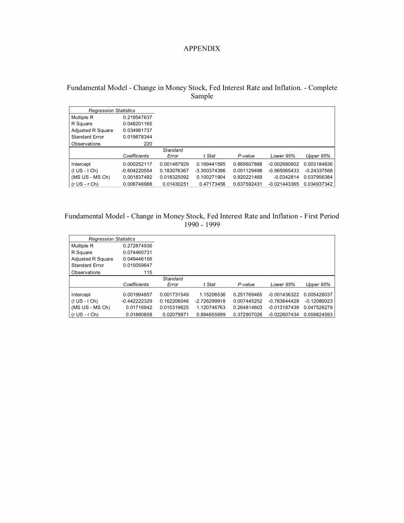
I. The first sets of regressions were performed utilizing the model described earlier that
includes the fundamental variables. The first test considers the complete sample
consisting of 220 monthly observations. The second regression was performed utilizing
the first period, from January 1990 until September 1999, where the exchange rate
regime changed. The third regression consists of the second period, from Sept 1999 to
March 2008.
The results for the first test are shown in Table 1 in the appendix.
In this case, for both change in monetary policy interest rates and change in money stock
coefficients, the null hypothesis has to be accepted. There is no statistical evidence that the
slope of these coefficients is significantly different from zero. However, for the differential in
Inflation, the Pvalue is 0.001129498 at a 5% confidence level.
The coefficients are:
) ( 4 0.60422055 7 0.00025211 $ CLP US t I I e − = ∆
If the American inflation differential is higher than the Chilean inflation differential, the
Chilean currency will appreciate. The adjusted R square for this test is 3.4981737%
For the second test performed we used 115 observations, where we do not have a
change in the monetary policy. Let´s remember that for this period the regime of the CCB
was inflation targeting.

16
The summary statistics for this test can be found in Table 2 in the appendix.
Once again, for both change in monetary policy interest rates and money stock
change, there is no statistical evidence that the slope of these coefficients is significantly
different from zero therefore the null hypothesis has to be accepted.
The Pvalue for ) ( $ CLP US I I − is 0.007445252, meaning that it’s statistically significant
at a 5% confidence level.
In this case, the coefficients are:
) ( 9 0.44222232 7 0.00199485 $ CLP US t I I e − = ∆
The adjusted R square for this regression is 4.9446156% and it is the highest in this
first set of tests performed.
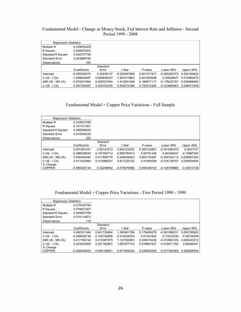
The third test performed considers the second period, after September ´99 and consists
of 105 observations. The summary statistics for this test are in Table 3.
We still do not find evidence that either the change in interest rates or money stocks
are significant determinants of the exchange rate, but MS has improved as an explanatory
variable.
The coefficients are:
) ( 7 1.28966289 75 0.0005393 $ CLP US t I I e − = ∆
Even if the coefficient for ) ( $ CLP US I I − is the highest, the pvalue is the less
significant (0.051925028, significant at a 6% confidence level) and the adjusted R square is
also the lowest (2.4737736%).
The results of these tests shows us that for the first half of the period studied, where
the objective of the central bank of Chile was to target and lower inflation, the inflation
differential had the greatest impact in the exchange rate determination, out of all variables
considered. In any of these regressions the other variables showed statistical significance in
the analysis.

17
A final regression was performed utilizing a Dummy variable for representing the regime
change occurred in 1999, but it does not add any statistical significance to the model. The
results for this regression can be found in Table 7 in the appendix.
II. For the second set of regressions, testing the second period, the change in copper
prices was added to the model to determine the influence that the commodity price
may have in foreign exchange determination. Copper is traded in the London
Mercantile Exchange. The data also consists in monthly observations and will be
separated just as in the tests performed previously. As mentioned earlier, copper
prices increased dramatically due to international inventory drops and increasing
international demand.
The model used this time is the following.
) % ( ) ( ) ( ) ( Pr 4 $
3 $
2 $
1 ice Copper CLP US CLP US CLP US
t r r I I MS MS e ∆ + − + − + − + = ∆ β β β β α
The summary statistics for the first set of tests can be found in Table 4 in the
appendix.
In this case, as we found in the first set of regressions, changes in the monetary policy
interest rate and changes in the money stock are not significant at a 5% confidence level.
There is no statistical evidence that the slope of these coefficients is significantly different
from zero, therefore the null hypothesis has to be accepted.
The coefficients are as follows,
) % ( 0.08042013 ) ( 0.48602805 1 0.00126316 Pr $
ice Copper CLP US
t I I e ∆ − = ∆
The Pvalue for ) ( $ CLP US I I − is 0.00791446 at a 5% confidence level, while for
) % ( Pr ice Copper ∆ the Pvalue is 0.000426143, making it statistically significant at a 5% level.
An increasing copper price would result in an appreciating currency, which is consistent with
our expectations.
Looking at the inflation effect, the results are similar to the ones obtained in the
previously tested regressions. If the change in the American inflation is higher than the
change in the Chilean inflation, the Chilean currency will appreciate.

18
The second regression test performed using this model considers the first period of the
sample, consisting of 115 monthly observations. The summary statistics for this regression
can be found in Table 5 in the appendix.
For this period of time, copper price remained fairly stable and without great
volatility. The PValue for this variable is 0.330662929; therefore it is not statistically
significant at a 5% confidence level. Since this variable does not add evidence of exchange
rates determination, the results are very similar to the ones obtained in the second regression
performed using the original model.
For the third regression, we utilized the observations for the second period of time. At
this point, copper prices suffered a rapid increase due to growing international demand and a
drop in inventory levels worldwide. Also our dependant variable t e ∆ started appreciating
after a prolonged depreciating trend.
The summary statistics for this regression can be found in Table 6 in the appendix.
The coefficients are;
) % ( 0.11440637 7 0.00125188 Pr ice Copper t e ∆ = ∆
In this case, and for the first time in our study, the differential on inflation levels is not
significant at a 5% confidence level, with a PValue of 0.258064303. On the other hand, the
PValue for the change in copper price is 0.003354111; making it highly significant. Once
again, results show us that an increasing copper price would result in an appreciating
currency. The adjusted R square coefficient is 10.2890058%, the highest obtained so far,
meaning that 10.29% of exchange rates movements are explained by variations in copper
price.
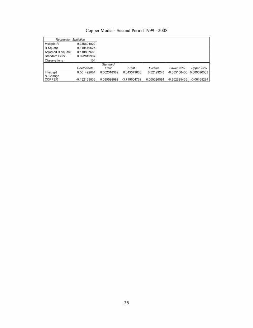
A new regression was performed using only the change in copper price variable and
excluding all other independent variables from the model. Summary statistics can be found in
table 8 for the full sample and table 9 for the second period.
Here we can see that the influence of copper for the second period studied is
considerably higher than for the full sample.
The coefficients for the regression using only the second period are shown below.
) % ( 5 0.13215383 4 0.00149206 Pr ice Copper t e ∆ = ∆
19
The adjusted R square value for the analysis using the full sample is 6.54%, and
increased to 11.08% when analyzing only the second period. The increased explanatory
power of this variable is clear.
Summarizing the results obtained so far, we can conclude that after splitting the data
in two periods, we find different exchange rate determinants in each one of them. The break
in the data was made in September 1999, where the central bank of Chile decided to modify
its foreign exchange rate policy. Before this period, the goal of the CCB was to target and
lower inflation, and precisely this is the variable that showed us the greatest role in the
exchange rate determination. The results shows us that all other independent variable
considered were not statistically significant in any of the regressions performed.
If the differential between the change in the US inflation and the change in the
Chilean inflation ) ( $ CLP US I I − is a negative value, then the CLP will depreciate. In other
words, if the Chilean inflation is higher than the US inflation in a certain period of time, we
can expect the Chilean currency to depreciate. That was the case for almost the complete
period from 1990 to 1999.
After adding a fourth variable to the model, the results showed us that the role of
copper in the exchange rate determination increased dramatically after year 2003. Before that
year, its average price was 94.62 US$/Lb. In the second half of the sample, its average price
was 218 US$/Lb, reaching its top price of 393 US$/Lb.
For this period (’99 ‘08), regression results showed that all other variables were not
statistically significant.
A positive variation in copper price will result in an appreciating currency.
Also the adjusted R square coefficient for this regression is 10.29%, being the highest
obtained so far.
The analysis showed us that money supply was never significant in any of the
regressions performed. This result was somehow expected because this model was also used
in the study by Grauwe and Vansteenkiste (2007) and they could not find significance for this
coefficient either.
It is interesting to notice that in one regime the variables in question may have a
significant effect on the exchange rate, while in other regime their effect is not significantly
different from zero. In this case, for the first period studied the significance of inflation is

20
evident, while for the second period this explanatory power is displaced by the influence of
copper prices.
The results are similar to the ones obtained by the earlier mentioned study by Grauwe
and Vansteenkiste (2007), where they performed similar tests to high and low inflation
countries. Let´s recall that in their study they could not find a relation between the
fundamentals and the currencies of low inflation nations, whereas this link was stable and
significant for high inflation countries.
This phenomenon is explained as follows. Transaction costs are present in traded
goods and define a band where arbitrage opportunities do not hold. This is the same for both,
high and low inflation countries. If exogenous shocks are introduced in the underlying
fundamentals for the low inflation countries, these shocks will usually tend to be small
relative to the transaction costs band (differential inflation shocks are typically 1% or 2% per
year), hence, arbitrage will not be profitable and will not take place. The connection between
the news in the fundamentals and the currencies for these countries will not be strong.
Moreover, if a shock is larger compared to the transaction cost band, arbitrage will take place,
but as a consequence the relationship between the fundamentals and the exchange rate will be
unstable.
On the other hand, for high inflation countries, shocks in the fundamental values tend to
be large compared to the transaction costs band, allowing for strong arbitrage relations. This
implies a stronger and more stable relationship between the fundamental values and the
foreign exchange rate.
III. The following analysis will consider daily exchange rates information and daily
copper prices starting Jan 1, 1990 to Jul 31, 2008. The objective for this new analysis
is to determine the time that it takes to the market to react to new copper prices and to
reflect these changes in the currency determination. The model used in this analysis is
derived from the Granger Casualty test and is basically a lagged linear regression. The
Granger causality is a statistical concept of causality that is based on prediction.
According to Granger causality, if a signal X “Grangercauses” (or “Gcauses”) a
signal Y, then past values of X should contain information that helps predict Y above
and beyond the information contained in past values of Y alone. In our study, we are
trying to find evidence in past values of copper prices and how long it takes to be
reflected in the currencies.

21
The model can be represented as follows;
) % ( ) % ( ) % ( ) % ( Pr 3 Pr 2 Pr 1 Pr ice Copper t ice Copper t ice Copper t ice Copper t t e ∆ + ∆ + ∆ + ∆ + = ∆ − − − β β β β α
Where USD CLP e t ∆
∆ = ∆
, t β represents the change in copper prices on the same day, 1 − t β
represents changes in copper prices the previous day and 2 − t β & 3 − t β represent two and three
days lag respectively.
Complete Summary statistics for this test can be found on table 16.
The coefficients are shown below.
Table 2. Lagged Regression Coefficients
Coefficients Standard Error t Stat Pvalue
Intercept 6.3873E05 0.000119192 0.535882148 0.592097026 Delta CP PR 0.008757582 0.007557047 1.158862886 0.246644469 Delta CP PR 1 0.078383687 0.007570042 10.35445843 1.54794E24 Delta CP PR 2 0.031023761 0.007570987 4.097717127 4.33174E05 Delta CP PR 3 0.013199982 0.007558277 1.746427518 0.080883586
• Delta CP PR (change in copper price)
These results show us that our variable t β is not significant at a 5% confidence level,
while 1 − t β and 2 − t β are significant. The null hypothesis has to b accepted for t β .
3 − t β is significant at a 10% confidence level.
The signs of 1 − t β and 2 − t β are expected, considering the results obtained in previous
sets of regressions using monthly data. An increase in copper price will lead to an
appreciating currency. The sign of 3 − t β may correspond to market adjustments after
variations in copper price.
The adjusted R square for this model is 5.6%.
The market would respond on average between one and two days after the variation in
copper price to reflect the new exchange rate.

22
CONCLUSION
Our research objective was to analyze the relationship between exchange rate changes
and the variations in the underlying fundamentals. We considered the Chilean peso, and
compared it to the US dollar. We tested the performance of this currency for the last eighteen
years.
The results show that the determinants of the exchange rate may vary over time. The
independent variables that have an effect on the exchange rate may lose their explanatory
power when economic conditions change or a switch in the foreign exchange rate policy
dictated by central banks or, as we proved, when variations on certain markets takes place.
The model that we used includes three dependable variables. Theory supports these
variables and incorporates them in their explanation on how exchange rates move over time.
These variables are the money supply (M2), changes in domestic price levels and monetary
policy interest rate.
The data corresponded to monthly observations for the independent variables for both
countries, The United States of America and Chile. This data set was analyzed as a whole in a
first stage and separated into two groups for a more detailed study. By taking a preliminary
look at the data, two natural break points appear. The first one takes place when the central
bank of Chile decided to change the foreign monetary policy regime. Before September 1999
the objective of the CCB was to target inflation. After that, they adopted a freely floating
exchange rate regime. The second breaking point takes place in March 2003, where the
Chilean peso reached his historical lowest level of 745.21 pesos per US Dollar. After running
simple linear regression analysis and comparing the results on both sample groups, we find
that the first data division explained in a better way the determinants of the Chilean peso
movements. The break in the long depreciating trend of the Chilean peso compared to the US
Dollar has different explanations that are not covered in this study, for example, the euro
community started utilizing € as their currency. That period (2003) was the initiation of a
process where the US Dollar lost value against many currencies, principally the €, £ and
Chinese ¥.
Once we defined our data split, we performed simple linear regressions utilizing the
model derived from the Markovswitching autoregressive (MSAR).
We find that for the first period (1990 1999) changes in price levels played a
significant role in the exchange rate determination. Both money supply and monetary policy

23
interest rate were found to be not significant in the analysis. For the second period (after the
switch in the exchange rate policy) we found that Inflation does not have the same
explanatory power as in the first period.
Our analysis continued including a fourth variable into our model. Copper plays a
great role in the Chilean Economy, as this country is the biggest producer and exporter of
copper worldwide. Exchange rate movements seem to move in concordance with variations
in international copper prices. The results of our regression analysis showed us that for the
first period, inflation continues to be the strongest variable in the determination of the
exchange rate. However, the strong augment in price that copper experienced starting in year
2000 shows us an increasing explanatory power of this variable. As copper prices boosted,
the influence of copper becomes more and more important in determining the value of the
Chilean peso. Our study showed us that for the second period, inflation is not significant
anymore and variations in international copper prices become our main dependable variable.
Our concluding analysis consisted in measuring the time that the market reacts to
variations in copper prices. For this, we performed a simple lagged regression derived from
the Grangercauses concept. On average, the market reflects the currency adjustments one
and two days after the price variations.

LITERATURE CITED
Econometric Approaches to empirical models of exchange rate determination, Blackwell Synergy
Foreign Exchange Market, theory and econometric evidence, by Richard T. Baillie Fx Trading and exchangerates dynamics, JSTOR
“Exchange Rates and fundamentals: A Non linear Relationship?” by Paul de Grawke and Isabel Vansteenkiste
Econometric models in the UK, P. G. Fisher, S. K. Tanna, D. S. Turner, K. F. Wallis, J. D. Whitley, JSTOR
Exchange Rate Theory: A Review By Dr. Pongsak Hoontrakul [Dec 99]
Recent Evolution on Exchange Rates, (LA EVOLUCIÓN RECIENTE DEL TIPO DE CAMBIO) By José de Gregorio, president of the Central Bank of Chile
“Exchange Rates and Fundamentals: Evidence on LongHorizon Predictability” by Nelson C. Mark, march 1995.
The Economist Intelligence Unit Limited 2007
APPENDIX
Fundamental Model Change in Money Stock, Fed Interest Rate and Inflation. Complete Sample
Regression Statistics Multiple R 0.219547637 R Square 0.048201165 Adjusted R Square 0.034981737 Standard Error 0.019878344 Observations 220
Coefficients Standard Error t Stat Pvalue Lower 95% Upper 95%
Intercept 0.000252117 0.001487929 0.169441595 0.865607888 0.002680602 0.003184836 (I US I Ch) 0.604220554 0.183076367 3.300374396 0.001129498 0.965065433 0.24337568 (MS US MS Ch) 0.001837492 0.018325092 0.100271904 0.920221469 0.0342814 0.037956384 (r US r Ch) 0.006746988 0.01430251 0.47173456 0.637592431 0.021443365 0.034937342
Fundamental Model Change in Money Stock, Fed Interest Rate and Inflation First Period 1990 1999
Regression Statistics Multiple R 0.272874936 R Square 0.074460731 Adjusted R Square 0.049446156 Standard Error 0.015059647 Observations 115
Coefficients Standard Error t Stat Pvalue Lower 95% Upper 95%
Intercept 0.001994857 0.001731549 1.15206536 0.251769465 0.001436322 0.005426037 (I US I Ch) 0.442222329 0.162206046 2.726299918 0.007445252 0.763644428 0.12080023 (MS US MS Ch) 0.01716942 0.015319625 1.120746763 0.264814603 0.013187439 0.047526279 (r US r Ch) 0.01860858 0.02079971 0.894655699 0.372907026 0.022607434 0.059824593
26
Fundamental Model Change in Money Stock, Fed Interest Rate and Inflation Second Period 1999 2008
Regression Statistics Multiple R 0.229935429 R Square 0.052870302 Adjusted R Square 0.024737736 Standard Error 0.023888785 Observations 105
Coefficients Standard Error t Stat Pvalue Lower 95% Upper 95%
Intercept 0.000539375 0.00238137 0.226497956 0.821271917 0.005263372 0.004184622 (I US I Ch) 1.289662897 0.655645047 1.967013863 0.051925028 2.59028627 0.010960475 (MS US MS Ch) 0.074231854 0.052527454 1.413201048 0.160671117 0.178432191 0.029968483 (r US r Ch) 0.007306387 0.020752335 0.352075398 0.725515264 0.033860663 0.048473436
Fundamental Model + Copper Price Variations Full Sample
Regression Statistics Multiple R 0.318937299 R Square 0.101721001 Adjusted R Square 0.085008833 Standard Error 0.019356235 Observations 220
Coefficients Standard Error t Stat Pvalue Lower 95% Upper 95%
Intercept 0.001263161 0.00147613 0.855724552 0.393102801 0.001646379 0.0041727 (I US I Ch) 0.486028054 0.181300713 2.680784013 0.00791446 0.84338247 0.12867364 (MS US MS Ch) 0.004456595 0.017858778 0.249546453 0.803176367 0.030744112 0.039657302 (r US r Ch) 0.011432884 0.013988257 0.817320122 0.41465029 0.016138797 0.039004564 % Change COPPER 0.080420134 0.02246952 3.579076586 0.000426143 0.124708885 0.03613138
Fundamental Model + Copper Price Variations First Period 1990 1999
Regression Statistics Multiple R 0.279334794 R Square 0.078027927 Adjusted R Square 0.044803708 Standard Error 0.015114873 Observations 116
Coefficients Standard Error t Stat Pvalue Lower 95% Upper 95%
Intercept 0.002331346 0.001725694 1.350961786 0.179455078 0.001088231 0.005750923 (I US I Ch) 0.409838736 0.162746808 2.518259755 0.01321942 0.73233239 0.08734508 (MS US MS Ch) 0.017789744 0.015367875 1.157592953 0.249515036 0.012662725 0.048242213 (r US r Ch) 0.023025809 0.021163861 1.087977733 0.278961637 0.018911792 0.06496341 % Change COPPER 0.025548833 0.026148621 0.977062324 0.330662929 0.077364069 0.026266404

27
Fundamental Model + Copper Price Variations Second Period 1999 2008
Regression Statistics Multiple R 0.371118956 R Square 0.137729279 Adjusted R Square 0.102890058 Standard Error 0.02292137 Observations 104
Coefficients Standard Error t Stat Pvalue Lower 95% Upper 95%
Intercept 0.001251887 0.0023965 0.522381164 0.602571956 0.00350329 0.006007063 (I US I Ch) 0.752811767 0.661797739 1.137525444 0.258064303 2.065962025 0.560338491 (MS US MS Ch) 0.051734457 0.051432206 1.00587669 0.316927118 0.153787109 0.050318195 (r US r Ch) 0.007737537 0.019915125 0.38852564 0.698461373 0.031778391 0.047253464 % Change COPPER 0.114406366 0.038058948 3.006030668 0.003354111 0.189923574 0.03888916
Fundamental Model + Copper + Dummy Variable for regime change Full Sample
Regression Statistics Multiple R 0.32004048 R Square 0.102425909 Adjusted R Square 0.081454551 Standard Error 0.019393794 Observations 220
Coefficients Standard Error t Stat Pvalue Lower 95% Upper 95%
Intercept 0.001919104 0.002178882 0.880774833 0.3794278 0.002375714 0.006213923 (I US I Ch) 0.455930382 0.195927656 2.327034329 0.020898258 0.842125581 0.06973518 (MS US MS Ch) 0.004188149 0.017905409 0.233904104 0.815283038 0.031105403 0.0394817 (r US r Ch) 0.010779153 0.014105824 0.764163276 0.445611688 0.017024995 0.0385833 % Change COPPER 0.079409514 0.022647686 3.506297012 0.000553507 0.124050622 0.03476841 RegDum 0.001177357 0.002871907 0.409956654 0.682247839 0.006838206 0.004483491
Copper Model Full Sample
Regression Statistics Multiple R 0.263983363 R Square 0.069687216 Adjusted R Square 0.065419726 Standard Error 0.019562338 Observations 220
Coefficients Standard Error t Stat Pvalue Lower 95% Upper 95%
Intercept 0.002968622 0.001329311 2.233203532 0.026551637 0.000348676 0.005588567 % Change COPPER 0.08963467 0.022181234 4.041013575 7.37842E05 0.133351788 0.04591755
28
Copper Model Second Period 1999 2008
Regression Statistics Multiple R 0.345601829 R Square 0.119440625 Adjusted R Square 0.110807689 Standard Error 0.022819997 Observations 104
Coefficients Standard Error t Stat Pvalue Lower 95% Upper 95%
Intercept 0.001492064 0.002318382 0.643579668 0.52129243 0.003106436 0.006090563 % Change COPPER 0.132153835 0.035528999 3.719604769 0.000326584 0.202625435 0.06168224

29
The Following four tables show the results obtained when splitting the data in the observation number 158 (February 2003) in the inflexion point of the currencies.
Fundamental Model Change in Money Stock, Fed Interest Rate and Inflation First Period 1990 2003
Regression Statistics Multiple R 0.188739591 R Square 0.035622633 Adjusted R Square 0.016713273 Standard Error 0.017752725 Observations 157
Coefficients Standard Error t Stat Pvalue Lower 95% Upper 95%
Intercept 0.004165401 0.001648171 2.527287265 0.012510028 0.000909291 0.007421511 (I US I Ch) 0.40019354 0.177860292 2.25004431 0.025872265 0.7515726 0.04881447 (MS US MS Ch) 0.009127144 0.017618362 0.518047267 0.605173597 0.02567952 0.043933809 (r US r Ch) 0.010593976 0.014103314 0.751169214 0.453704644 0.0172684 0.038456346
Fundamental Model Change in Money Stock, Fed Interest Rate and Inflation Second Period 2003 2008
Regression Statistics Multiple R 0.15245748 R Square 0.023243283 Adjusted R Square 0.02642231 Standard Error 0.023013459 Observations 63
Coefficients Standard Error t Stat Pvalue Lower 95% Upper 95%
Intercept 0.00690401 0.002963606 2.32959753 0.023269662 0.01283417 0.00097385 (I US I Ch) 0.63486799 0.733919522 0.86503761 0.390521842 2.10343755 0.833701571 (MS US MS Ch) 0.04117006 0.057515706 0.71580547 0.476934981 0.15625872 0.073918604 (r US r Ch) 0.01232468 0.039370278 0.3130452 0.755350259 0.09110442 0.066455067

30
Fundamental Model + Copper Price Variations First Period 1990 2003
Regression Statistics Multiple R 0.22732449 R Square 0.051676424 Adjusted R Square 0.02672054 Standard Error 0.017662156 Observations 157
Coefficients Standard Error t Stat Pvalue Lower 95% Upper 95%
Intercept 0.004263683 0.001640906 2.598370651 0.010288394 0.001021754 0.007505612 (I US I Ch) 0.37283555 0.177772897 2.09725753 0.037626114 0.72406037 0.02161072 (MS US MS Ch) 0.009800577 0.017533505 0.558962805 0.577009695 0.02484026 0.044441416 (r US r Ch) 0.013333015 0.014134879 0.943270577 0.347039391 0.01459318 0.041259208 % Change COPPER 0.04557351 0.028410583 1.60410324 0.110767126 0.10170412 0.010557107
Fundamental Model + Copper Price Variations Second Period 2003 2008
Regression Statistics Multiple R 0.326640577 R Square 0.106694066 Adjusted R Square 0.045086761 Standard Error 0.022197334
Observations 63
Coefficients Standard Error t Stat Pvalue Lower 95% Upper 95%
Intercept 0.0041939 0.003086521 1.35877872 0.179477674 0.01037224 0.001984444 (I US I Ch) 0.08051803 0.746879139 0.10780597 0.914521681 1.57555905 1.414522993 (MS US MS Ch) 0.02524864 0.055896106 0.45170656 0.65316506 0.13713685 0.086639575 (r US r Ch) 0.01005051 0.037986658 0.26458 0.792270997 0.08608907 0.065988047
% Change COPPER 0.09385988 0.040322822 2.3277112 0.023437755 0.17457478 0.01314499
Lagged Regression derived from the Granger Casualty test Daily data Jan 2000 Jul 2008
Regression Statistics Multiple R 0.240508217 R Square 0.057844202 Adjusted R Square 0.056041033 Standard Error 0.005422683 Observations 2095
Coefficients Standard Error t Stat Pvalue Lower 95% Upper 95%
Intercept 6.3873E05 0.000119192 0.535882148 0.592097026 0.00016987 0.000297621 Delta CP PR 0.008757582 0.007557047 1.158862886 0.246644469 0.00606254 0.023577705 Delta CP PR 1 0.07838369 0.007570042 10.3544584 1.54794E24 0.09322929 0.06353808 Delta CP PR 2 0.03102376 0.007570987 4.09771713 4.33174E05 0.04587122 0.0161763 Delta CP PR 3 0.013199982 0.007558277 1.746427518 0.080883586 0.00162255 0.028022516

31
Exchange Rate Volatility
Copper Price Volatility
Inflation Volatility
‐0.08 ‐0.06 ‐0.04 ‐0.02
0 0.02 0.04 0.06 0.08
1990
19
90
1991
19
91
1992
19
93
1993
19
94
1994
19
95
1995
19
96
1997
19
97
1998
19
98
1999
20
00
2000
20
01
2001
20
02
2002
20
03
2004
20
04
2005
20
05
2006
20
07
2007
20
08
Exchange Rate Volatility
‐0.3
‐0.2
‐0.1
0 0.1
0.2
0.3
1990
19
90
1991
19
91
1992
19
93
1993
19
94
1994
19
95
1995
19
96
1997
19
97
1998
19
98
1999
20
00
2000
20
01
2001
20
02
2002
20
03
2004
20
04
2005
20
05
2006
20
07
2007
20
08
Copper Price Volatility
‐0.05 ‐0.04 ‐0.03 ‐0.02 ‐0.01
0 0.01 0.02 0.03 0.04
1990
19
90
1991
19
91
1992
19
93
1993
19
94
1994
19
95
1995
19
96
1997
19
97
1998
19
98
1999
20
00
2000
20
01
2001
20
02
2002
20
03
2004
20
04
2005
20
05
2006
20
07
2007
20
08
Inflation Volatility


