
Department of Civil and Environmental Engineering Stanford University
MODELING OF EARTHQUAKE GROUND MOTION IN THE FREQUENCY DOMAIN
by
Hjörtur Thráinsson,
Anne S. Kiremidjian
and
Steven R. Winterstein
Report No. 134 June 2000

The John A. Blume Earthquake Engineering Center was established to promote research and education in earthquake engineering. Through its activities our understanding of earthquakes and their effects on mankind’s facilities and structures is improving. The Center conducts research, provides instruction, publishes reports and articles, conducts seminar and conferences, and provides financial support for students. The Center is named for Dr. John A. Blume, a well-known consulting engineer and Stanford alumnus. Address: The John A. Blume Earthquake Engineering Center Department of Civil and Environmental Engineering Stanford University Stanford CA 94305-4020 (650) 723-4150 (650) 725-9755 (fax) earthquake @ce. stanford.edu http://blume.stanford.edu
©2000 The John A. Blume Earthquake Engineering Center

MODELING OF EARTHQUAKE GROUND MOTION
IN THE FREQUENCY DOMAIN
by
Hjörtur Thráinsson
Anne S. Kiremidjian
and
Steven R. Winterstein
This research was partially supported
by
The John A. Blume Earthquake Engineering Center
The National Science Foundation Grant No. CMS-5926102
and
The Stanford University UPS Foundation Grant
The John A. Blume Earthquake Engineering Center
Department of Civil and Environmental Engineering
Stanford University, Stanford, CA 94305-4020
Report No. 134
May 2000

© Copyright by Hjörtur Thráinsson 2000
All Rights Reserved
Abstract iii
ABSTRACT
In recent years, the utilization of time histories of earthquake ground motion has grown
considerably in the design and analysis of civil structures. It is very unlikely, however,
that recordings of earthquake ground motion will be available for all sites and conditions
of interest. Hence, there is a need for efficient methods for the simulation and spatial
interpolation of earthquake ground motion. In addition to providing estimates of the
ground motion at a site using data from adjacent recording stations, spatially interpolated
ground motions can also be used in design and analysis of long-span structures, such as
bridges and pipelines, where differential movement is important.
The objective of this research is to develop a methodology for rapid generation of
horizontal earthquake ground motion at any site for a given region, based on readily
available source, path and site characteristics, or (sparse) recordings. The research
includes two main topics: (i) the simulation of earthquake ground motion at a given site,
and (ii) the spatial interpolation of earthquake ground motion.
In topic (i), models are developed to simulate acceleration time histories using the
inverse discrete Fourier transform. The Fourier phase differences, defined as the
difference in phase angle between adjacent frequency components, are simulated
conditional on the Fourier amplitude. Uniformly processed recordings from recent
California earthquakes are used to validate the simulation models, as well as to develop
prediction formulas for the model parameters. The models developed in this research
provide rapid simulation of earthquake ground motion over a wide range of magnitudes
and distances, but they are not intended to replace more robust geophysical models.
In topic (ii), a model is developed in which Fourier amplitudes and Fourier phase
angles are interpolated separately. A simple dispersion relationship is included in the
phase angle interpolation. The accuracy of the interpolation model is assessed using data
from the SMART-1 array in Taiwan. The interpolation model provides an effective
method to estimate ground motion at a site using recordings from stations located up to
several kilometers away. Reliable estimates of differential ground motion are restricted to
relatively limited ranges of frequencies and inter-station spacings.


Acknowledgments v
ACKNOWLEDGMENTS
This report is based on the doctoral dissertation of Hjörtur Thráinsson. The research was
partially supported by the John A. Blume Earthquake Engineering Center, the National
Science Foundation Grant No. CMS-5926102, and the Stanford University UPS
Foundation Grant. This support is gratefully acknowledged.
Several people contributed to this research. Feedback from participants in the annual
meetings of the Reliability of Marine Structures Program at Stanford University was very
helpful. Conversations with Bill Joyner at the U.S. Geological Survey in Menlo Park
were also beneficial. Professor Greg Beroza, Department of Geophysics at Stanford
University, reviewed the manuscript. The advice of these individuals is gratefully
appreciated.


Table of Contents vii
TABLE OF CONTENTS
ABSTRACT .................................................................................................................... III
ACKNOWLEDGMENTS ............................................................................................... V
TABLE OF CONTENTS..............................................................................................VII
LIST OF TABLES ..........................................................................................................XI
LIST OF FIGURES .................................................................................................... XIII
1 INTRODUCTION.........................................................................................................1
1.1 BACKGROUND ..........................................................................................................11.2 OBJECTIVE AND SCOPE.............................................................................................71.3 ORGANIZATION OF THE REPORT...............................................................................7
2 DATA AND DATA PROCESSING.............................................................................9
2.1 THE GROUND MOTION DATA SET ............................................................................92.1.1 Ground Motion Recordings.............................................................................92.1.2 Data Processing ............................................................................................112.1.3 Site Classification According to Soil Conditions ..........................................13
2.2 THE REGRESSION PROCEDURE ...............................................................................14
3 MODELING OF PHASE DIFFERENCES: PARAMETRIC METHOD .............19
3.1 THE DISCRETE FOURIER TRANSFORM ....................................................................193.2 CHARACTERIZATION OF FOURIER PHASE DIFFERENCES .........................................203.3 MODEL PARAMETERS.............................................................................................27
3.3.1 Fundamental Parameters ..............................................................................303.3.2 Secondary Parameters ..................................................................................38
3.4 MODEL VALIDATION..............................................................................................433.4.1 Phase Difference Distributions .....................................................................443.4.2 Accelerograms...............................................................................................46
3.5 SUMMARY OF CONDITIONAL BETA DISTRIBUTIONS ...............................................50
4 MODELING OF PHASE DIFFERENCES: METHOD OF ENVELOPES..........53
4.1 THE HILBERT TRANSFORM.....................................................................................544.2 ENVELOPES OF TIME-VARYING FUNCTIONS...........................................................554.3 ENVELOPES OF FREQUENCY-VARYING FUNCTIONS................................................58

Table of Contentsviii
4.4 PARAMETER ESTIMATION.......................................................................................634.5 MODEL PARAMETERS.............................................................................................68
4.5.1 The First Whitened Intensity Moment ...........................................................734.5.2 The Second Whitened Intensity Moment .......................................................77
4.6 MODEL VALIDATION..............................................................................................804.6.1 Phase Difference Distributions .....................................................................804.6.2 Accelerograms...............................................................................................88
4.7 SUMMARY OF CONDITIONAL NORMAL DISTRIBUTIONS..........................................91
5 MODELING OF FOURIER AMPLITUDES...........................................................93
5.1 CURRENT AMPLITUDE MODELS .............................................................................935.1.1 Radiated Source Spectrum ............................................................................945.1.2 Filtered Kanai-Tajimi Spectrum ...................................................................97
5.2 LOGNORMAL DENSITY FUNCTION AS AMPLITUDE SPECTRUM................................985.3 MODEL PARAMETERS...........................................................................................100
5.3.1 The Energy Parameter ................................................................................1035.3.2 The Central Frequency Parameter..............................................................1065.3.3 The Spectral Bandwidth Parameter ............................................................1095.3.4 Examples of Predicted Fourier Amplitude Spectra.....................................111
5.4 SUMMARY OF AMPLITUDE MODELS .....................................................................113
6 SPATIAL INTERPOLATION OF GROUND MOTION .....................................117
6.1 PROBLEM STATEMENT AND BASIC ASSUMPTIONS................................................1186.2 DATA AND DATA PROCESSING .............................................................................119
6.2.1 The SMART-1 Array....................................................................................1206.2.2 Data.............................................................................................................1216.2.3 Geometric Interpolation Schemes ...............................................................122
6.3 INTERPOLATION OF DISCRETE FOURIER TRANSFORMS.........................................1246.3.1 Methods for Averaging Complex Numbers .................................................1266.3.2 Interpolation of Fourier Amplitudes ...........................................................1346.3.3 Interpolation of Fourier Phase Angles........................................................142
6.4 INTERPOLATED TIME HISTORIES ..........................................................................1576.5 DELAUNAY TRIANGULATION ...............................................................................1696.6 SUMMARY OF SPATIAL INTERPOLATION...............................................................170
7 CASE STUDY: THE NORTHRIDGE EARTHQUAKE ......................................173
7.1 GROUND MOTION INTENSITY MAPS.....................................................................1757.2 INTERPOLATION OF TIME HISTORIES ....................................................................181
7.2.1 Three-Point Interpolation ...........................................................................1827.2.2 Effects of the Apparent Phase Velocity .......................................................1897.2.3 Two-Point Interpolation..............................................................................191

Table of Contents ix
8 SUMMARY AND CONCLUSIONS........................................................................199
8.1 SUMMARY ............................................................................................................1998.2 CONCLUSIONS ......................................................................................................2018.3 FUTURE WORK.....................................................................................................204
APPENDIX A: CALIFORNIA RECORDING STATIONS ....................................207
APPENDIX B: DATA; PARAMETRIC METHOD.................................................213
APPENDIX C: DATA; METHOD OF ENVELOPES .............................................219
APPENDIX D: DATA; FOURIER AMPLITUDES .................................................227
APPENDIX E: STATIONS IN THE SMART-1 ARRAY........................................235
APPENDIX F: CASE STUDY; RECORDINGS AND SIMULATIONS.................237
REFERENCES ..............................................................................................................243


List of Tables xi
LIST OF TABLES
Table 2.1: The California earthquakes and the number of ground motionrecording stations that are used in this study. 10
Table 2.2: Definition of NEHRP Site Classes. 14
Table 3.1: Regression results for the mean normalized phase difference forlarge Fourier amplitudes. 33
Table 3.2: Regression results for the variance of normalized phase differencefor small Fourier amplitudes. 37
Table 3.3: Critical values of the Kolmogorov-Smirnov statistic for normalizedphase difference distributions. 45
Table 4.1: The frequency domain analogy to the method of envelopes. 61Table 4.2: Regression results for the first whitened intensity moment. 75Table 4.3: Regression results for the second whitened intensity moment. 79Table 4.4: Critical values of the two-sample Kolmogorov-Smirnov statistic for
phase difference distributions. 86
Table 5.1: Regression results for the energy parameter. 106Table 5.2: Regression results for the central frequency parameter. 107Table 5.3: Regression results for the spectral bandwidth parameter. 111
Table 6.1: Shear wave velocity profile at the SMART-1 array site. 121Table 6.2: Events recorded by the SMART-1 array that are used in this study. 122
Table A.1: California recording stations that are used in this study. 208Table B.1: Statistics on normalized phase differences that are used in Chapter 3. 214Table C.1: The whitened intensity moments that are used in Chapter 4. 220Table D.1: The Fourier spectra parameters that are used in Chapter 5. 228Table E.1: SMART-1 array station locations. 235Table F.1: Recorded peak ground accelerations in the 1994 Northridge
earthquake and summary statistics of simulated peak groundaccelerations. 238
Table F.2: Recorded spectral accelerations corresponding to a natural period of0.3 sec in the 1994 Northridge earthquake and summary statisticsfrom 10 simulations. 239
Table F.3: Recorded spectral accelerations corresponding to a natural period of1.0 sec in the 1994 Northridge earthquake and summary statisticsfrom 10 simulations. 240
Table F.4: Recorded spectral accelerations corresponding to a natural period of2.0 sec in the 1994 Northridge earthquake and summary statisticsfrom 10 simulations. 241


List of Figures xiii
LIST OF FIGURES
Figure 2.1: The magnitude-distance combination of the California strong motionrecords. .........................................................................................................11
Figure 2.2: The gain function for a second order bi-directional Butterworth low-cutfilter. .............................................................................................................12
Figure 2.3: Shortest distance from site to vertical surface projection of seismogenicrupture. .........................................................................................................15
Figure 2.4: Schematic diagram of the two-step regression procedure............................17
Figure 3.1: Observed phase angles and phase differences..............................................22Figure 3.2: Histograms of phase differences for different amplitude categories............24Figure 3.3: Fitted and observed conditional phase difference distributions. ..................26Figure 3.4: Relationships between average normalized phase differences.....................28Figure 3.5: Relationships between the variances of normalized phase differences........29Figure 3.6: The weight of the uniform distribution as function of the variance of
normalized phase difference for small Fourier amplitudes. .........................30Figure 3.7: Mean normalized phase difference for large Fourier amplitudes as
function of distance, for two different earthquake magnitudes....................31Figure 3.8: Results of a two step regression analysis for the mean normalized phase
difference for large Fourier amplitudes and all sites....................................33Figure 3.9: Results of a two step regression analysis for the mean normalized phase
difference for large Fourier amplitudes and different site classes................34Figure 3.10: Variance of normalized phase difference for small Fourier amplitudes
as function of distance..................................................................................35Figure 3.11: Results of a two step regression analysis for the natural logarithm of the
variance of normalized phase difference for small Fourier amplitudesand all sites. ..................................................................................................36
Figure 3.12: Results of a two step regression analysis for the variance of normalizedphase difference for small Fourier amplitudes and different site classes.....37
Figure 3.13: Regression results for mean phase differences.............................................39Figure 3.14: Results of regression analysis of variance of normalized phase
difference for intermediate amplitudes vs. variance of normalizedphase difference for small amplitudes..........................................................40
Figure 3.15: Results of regression analysis of variance of normalized phasedifference for large amplitudes vs. variance of normalized phasedifference for small amplitudes....................................................................41
Figure 3.16: Results of regression analysis for the weight of the uniform distributionversus the variance of normalized phase difference for small Fourieramplitudes.. ..................................................................................................43
Figure 3.17: Comparison of observed phase difference distributions and fitteddistributions for small, intermediate and large Fourier amplitudes..............46
List of Figuresxiv
Figure 3.18: A recorded time history compared to two examples of simulatedtime histories using conditional beta distributions for Fourier phasedifferences. ...................................................................................................47
Figure 3.19: Elastic pseudo acceleration response spectra (5% damping) ofrecorded and simulated accelerograms using conditional betadistributions for Fourier phase differences...................................................48
Figure 3.20: Cumulative normalized Arias intensities of recorded and simulatedaccelerograms using conditional beta distributions for Fourier phasedifferences. ...................................................................................................49
Figure 4.1: Conditional mean and mean +/- one standard deviation of normalizedinstantaneous frequency as function of normalized amplitude. ...................57
Figure 4.2: An example of an amplitude modulated process..........................................59Figure 4.3: The whitening of an accelerogram ...............................................................65Figure 4.4: Histograms of the standardized real and imaginary parts ............................66Figure 4.5: Scatterplot of the standardized imaginary part versus the standardized
real part.........................................................................................................67Figure 4.6: Observed unwrapped phase differences as function of the whitened
Fourier amplitude. ........................................................................................67Figure 4.7: The second whitened intensity moment as function of the first whitened
intensity moment. .........................................................................................69Figure 4.8: The whitened duration parameter versus distance .......................................70Figure 4.9: The centroid of the whitened intensity function versus distance. ................70Figure 4.10: The centroid of the whitened intensity function versus the centroid of
the recorded intensity function. ....................................................................71Figure 4.11: The whitened duration parameter versus the recorded duration parameter. 71Figure 4.12: Results of a two step regression analysis for the first whitened intensity
moment and all sites .....................................................................................74Figure 4.13: Results of a two-step regression analysis for the first whitened intensity
moment and different site classes.................................................................75Figure 4.14: Results of a polynomial regression of the second whitened intensity
moment as function of the first whitened intensity moment ........................77Figure 4.15: Results of a linear regression in natural logarithm space for the second
whitened envelope moment as function of the first whitened envelopemoment.........................................................................................................78
Figure 4.16: Results of a linear regression of the second whitened intensity momentversus the first whitened intensity moment for different site classes...........79
Figure 4.17: Comparison of recorded and simulated Fourier phase angles and phasedifferences ....................................................................................................81
Figure 4.18: Cumulative probability distribution functions for recorded and simulatedphase angles..................................................................................................83
Figure 4.19: Standardization of phase differences............................................................85Figure 4.20: Cumulative probability distribution functions for the standardized phase
differences corresponding to a recorded and a simulated accelerogram......87Figure 4.21: Examples of simulated accelerograms using a conditional normal
distribution for the Fourier phase differences. .............................................88

List of Figures xv
Figure 4.22: Elastic pseudo acceleration response spectra (5% damping) of recordedand simulated accelerograms using a conditional normal distribution forthe Fourier phase differences .......................................................................89
Figure 4.23: Cumulative normalized Arias intensities of recorded and simulatedaccelerograms using a conditional normal distribution for the Fourierphase differences ..........................................................................................90
Figure 5.1: Schematic representation of the Fourier amplitude spectrum forearthquake ground acceleration (Equation 5.1) in logarithmic space. .........96
Figure 5.2: A low-cut filtered Kanai-Tajimi power spectral density as function ofnormalized frequency...................................................................................98
Figure 5.3: Scaled recorded Fourier amplitudes versus normalized frequency and the fitted truncated lognormal probability density function.......................100
Figure 5.4: The relationship between the two spectral moments for the Californiaground motion database; the spectral bandwidth parameter as functionof the central frequency parameter.............................................................102
Figure 5.5: The energy parameter as function of the central frequency parameter ......103Figure 5.6: Results of a two step regression analysis for the energy parameter and
all sites........................................................................................................105Figure 5.7: Results of a two-step regression analysis for the energy parameter for
different site classes....................................................................................105Figure 5.8: Results of a two-step regression analysis for the central frequency
parameter and all sites ................................................................................108Figure 5.9: Results of a two-step regression analysis for the central frequency
parameter for different site classes. ............................................................108Figure 5.10: Results of a linear regression of the spectral bandwidth parameter
versus the central frequency parameter for all sites.. .................................110Figure 5.11: Results of a linear regression of the spectral bandwidth parameter
versus the central frequency parameter for different site classes.. .............110Figure 5.12: Examples of predicted Fourier amplitude spectra......................................112
Figure 6.1: Schematic representation of the spatial interpolation problem ..................118Figure 6.2: The geometry of the SMART-1 accelerometer array in Lotung, Taiwan. .120Figure 6.3: Equilateral inner circle triangle to predict values at the central station. ....123Figure 6.4: Isosceles triangle to predict values at the inner circle stations...................124Figure 6.5: Averaging the complex numbers Z1 and Z2................................................126Figure 6.6: The recorded acceleration time history at station C-00 and the
interpolated time history using all the recording stations of theinner circle, obtained by averaging the real and imaginary partsof the DFT’s separately. .............................................................................128
Figure 6.7: The recorded Fourier amplitude spectrum at C-00 compared to thespectrum of the interpolated time history using all the recordingstations of the inner circle, obtained by averaging the real and theimaginary parts of the DFT’s separately. ...................................................128
Figure 6.8: The recorded Fourier phase angle spectrum at C-00 compared to thephase angle spectrum of the interpolated time history using all the
List of Figuresxvi
recording stations of the inner circle, obtained by averaging the realand the imaginary parts of the DFT’s separately. ......................................129
Figure 6.9: The recorded acceleration time history at station C-00 and theinterpolated time history using all the recording stations of the innercircle, obtained by evaluating the geometric mean of the Fourieramplitudes, but inferring the Fourier phase angles from averaging thereal and imaginary parts separately. ...........................................................130
Figure 6.10: The recorded Fourier amplitude spectrum at C-00 compared to theinterpolated spectrum using all the recording stations of the innercircle, obtained by evaluating the geometric mean. ...................................130
Figure 6.11: The cumulative normalized Arias intensity of the recording at C-00compared to the cumulative normalized Arias intensity of theinterpolated time history in Figure 6.9. ......................................................131
Figure 6.12: The recorded acceleration time history at station C-00 and theinterpolated time history using all the recording stations of the innercircle, obtained by averaging the squared Fourier amplitudes, butinferring the Fourier phase angles from averaging the real andimaginary parts separately..........................................................................132
Figure 6.13: The recorded Fourier amplitude spectrum at C-00 compared to theinterpolated spectrum using all the recording stations of the innercircle, obtained by averaging the squared Fourier amplitudes...................132
Figure 6.14: The cumulative normalized Arias intensity of the recording at C-00compared to the cumulative normalized Arias intensity of theinterpolated time history in Figure 6.12. ....................................................133
Figure 6.15: Averaging complex numbers. The results of the proposed methodcompared to results obtained by averaging the real and the imaginaryparts separately and by evaluating the geometric mean. ............................134
Figure 6.16: The recorded Fourier amplitude spectrum at station C-00 comparedto the interpolated spectrum using the station pair (I-03,I-09)...................136
Figure 6.17: The recorded Fourier amplitude spectrum at station C-00 comparedto the interpolated spectrum using the station pair (M-03,M-09). .............136
Figure 6.18: The recorded Fourier amplitude spectrum at station C-00 comparedto the interpolated spectrum using the station pair (O-03,O-09)................137
Figure 6.19: The recorded Fourier amplitude spectrum at station C-00 comparedto the interpolated spectrum using the triangle (I-03,I-07,I-11).................138
Figure 6.20: The recorded Fourier amplitude spectrum at station C-00 comparedto the interpolated spectrum using the triangle (M-03,M-07,M-11). .........138
Figure 6.21: The recorded Fourier amplitude spectrum at station C-00 comparedto the interpolated spectrum using the triangle (O-03,O-07,O-11). ...........139
Figure 6.22: The recorded Fourier amplitude spectrum at station C-00 comparedto the interpolated spectrum using all inner circle stations. .......................140
Figure 6.23: The recorded Fourier amplitude spectrum at station C-00 comparedto the interpolated spectrum using all middle circle stations. ....................140
Figure 6.24: The recorded Fourier amplitude spectrum at station C-00 compared to the interpolated spectrum using all outer circle stations. .......................141

List of Figures xvii
Figure 6.25: The recorded Fourier phase angle spectrum at station C-00 comparedto the interpolated phase spectrum using the propagation-perpendicularinner circle station pair (I-03,I-09). ............................................................144
Figure 6.26: The Fourier phase angle interpolation error at station C-00 for thepropagation-perpendicular inner circle station pair (I-03,I-09)..................145
Figure 6.27: The recorded Fourier phase angle spectrum at station C-00 comparedto the interpolated phase spectrum using the propagation-parallel innercircle station pair (I-06,I-12). .....................................................................146
Figure 6.28: The Fourier phase angle interpolation error at station C-00 for thepropagation-parallel inner circle station pair (I-06,I-12)............................147
Figure 6.29: The recorded Fourier phase angle spectrum at station C-00 comparedto the interpolated phase spectrum using the propagation-perpendicularmiddle circle station pair (M-03,M-09)......................................................148
Figure 6.30: The recorded Fourier phase angle spectrum at station C-00 comparedto the interpolated phase spectrum using the inner circle triangle(I-03,I-07,I-11). ..........................................................................................150
Figure 6.31: The Fourier phase angle interpolation error at station C-00 for the innercircle triangle (I-03,I-07,I-11). ...................................................................151
Figure 6.32: The recorded Fourier phase angle spectrum at station C-00 comparedto the interpolated phase spectrum using the middle circle triangle(M-03,M-07,M-11).....................................................................................152
Figure 6.33: The recorded Fourier phase angle spectrum at station C-00 comparedto the interpolated phase spectrum using all stations in the inner circle. ...154
Figure 6.34: The Fourier phase angle interpolation error at station C-00 using allstations in the inner circle...........................................................................155
Figure 6.35: The recorded Fourier phase angle spectrum at station C-00 compared tothe interpolated phase spectrum using all stations in the middle circle. ....156
Figure 6.36: The recorded acceleration time history at station C-00 and interpolatedtime histories using two diagonally opposite inner circle stations.............158
Figure 6.37: The cumulative normalized Arias intensities of the recording at stationC-00 and the two interpolated time histories from Figure 6.36. ................159
Figure 6.38: The recorded acceleration time history at station C-00 and interpolatedtime histories using a pair of propagation-perpendicular stations..............160
Figure 6.39: The cumulative normalized Arias intensities of the recording at stationC-00 and the two interpolated time histories from Figure 6.38. ................160
Figure 6.40: The recorded acceleration time history at station C-00 and interpolatedtime histories using inner circle triangles...................................................162
Figure 6.41: The cumulative normalized Arias intensities of the recording at stationC-00 and the three interpolated time histories from Figure 6.40. ..............162
Figure 6.42: The recorded acceleration time history at station C-00 and interpolatedtime histories using equilateral triangles (stations 03, 07, and 11). ...........164
Figure 6.43: The cumulative normalized Arias intensities of the recording at stationC-00 and the three interpolated time histories from Figure 6.42. ..............164
Figure 6.44: The recorded acceleration time history at station C-00 and interpolatedtime histories using all the recording stations in a given circle..................166

List of Figuresxviii
Figure 6.45: The cumulative normalized Arias intensities of the recording at stationC-00 and the three interpolated time histories from Figure 6.44. ..............166
Figure 6.46: The recorded acceleration time history at station C-00 and interpolatedtime histories using recordings from stations in the middle circle.............168
Figure 6.47: The cumulative normalized Arias intensities of the recording at stationC-00 and the three interpolated time histories from Figure 6.46. ..............168
Figure 6.48: Delaunay Triangulation..............................................................................170
Figure 7.1: A map showing the location of the recording stations used in thischapter. .......................................................................................................174
Figure 7.2: Statistics (from ten simulations) of peak ground acceleration asfunctions of the recorded peak ground acceleration for the east-westcomponent at 45 stations in the 1994 Northridge earthquake. ...................176
Figure 7.3: Statistics (from ten simulations) of spectral acceleration, correspondingto a natural period of 0.3 sec, as functions of the recorded spectralacceleration for the east-west component at 45 stations in the 1994Northridge earthquake................................................................................176
Figure 7.4: Statistics (from ten simulations) of spectral acceleration, correspondingto a natural period of 1.0 sec, as functions of the recorded spectralacceleration for the east-west component at 45 stations in the 1994Northridge earthquake................................................................................177
Figure 7.5: Statistics (from ten simulations) of spectral acceleration, correspondingto a natural period of 2.0 sec, as functions of the recorded spectralacceleration for the east-west component at 45 stations in the 1994Northridge earthquake................................................................................177
Figure 7.6: A contour map showing recorded and simulated peak groundacceleration for the east-west component in the 1994 Northridgeearthquake. .................................................................................................179
Figure 7.7: A contour map showing recorded and simulated spectral acceleration,corresponding to a natural period of 0.3 sec, for the east-westcomponent in the 1994 Northridge earthquake. .........................................179
Figure 7.8: A contour map showing recorded and simulated spectral acceleration,corresponding to a natural period of 1.0 sec, for the east-westcomponent in the 1994 Northridge earthquake. .........................................180
Figure 7.9: A contour map showing recorded and simulated spectral acceleration,corresponding to a natural period of 2.0 sec, for the east-westcomponent in the 1994 Northridge earthquake. .........................................180
Figure 7.10: A map showing the major highways in the Los Angeles region................182Figure 7.11: The east-west component of the recorded acceleration time histories at
stations LCN, HSL and BHA, and the interpolated time history. .............184Figure 7.12: The elastic, 5% damped, pseudo acceleration response spectra for the
east-west component of the recorded acceleration time histories atstations LCN, HSL and BHA, and for the interpolated time history. ........185
Figure 7.13: Cumulative normalized Arias intensity for the east-west componentof the recorded acceleration time histories at stations LCN, HSL andBHA, and for the interpolated time history................................................185
List of Figures xix
Figure 7.14: The north-south component of the recorded acceleration time historiesat stations LCN, HSL and BHA, and the interpolated time history. ..........187
Figure 7.15: The elastic, 5% damped, pseudo acceleration response spectra for thenorth-south component of the recorded acceleration time histories atstations LCN, HSL and BHA, and for the interpolated time history. ........188
Figure 7.16: Cumulative normalized Arias intensity for the north-south componentof the recorded acceleration time histories and for the interpolated timehistory.........................................................................................................188
Figure 7.17: Interpolated acceleration time histories, using the east-west componentof recordings at stations LCN, HSL and BHA, but three differentapparent phase velocities............................................................................190
Figure 7.18: The elastic, 5% damped, pseudo acceleration response spectra for thetime histories in Figure 7.17.......................................................................190
Figure 7.19: The cumulative normalized Arias intensities for the time histories inFigure 7.17..................................................................................................191
Figure 7.20: The east-west component of the recorded acceleration time histories atstations LCN and BHA, and the interpolated time history.........................192
Figure 7.21: The elastic, 5% damped pseudo acceleration response spectra for theeast-west component of the recorded time histories at stations LCNand BHA, and for the interpolated time history. ........................................193
Figure 7.22: The cumulative, normalized Arias intensities for the east-westcomponent of the recorded acceleration time histories at stations LCNand BHA, and for the interpolated time history .........................................193
Figure 7.23: The north-south component of the recorded acceleration time historiesat stations LCN and BHA, and the interpolated time history.....................194
Figure 7.24: Elastic, 5% damped pseudo acceleration response spectra for thenorth-south component of the recorded acceleration time histories atstations LCN and BHA, and for the interpolated time history...................195
Figure 7.25: Cumulative normalized Arias intensities for the north-south componentof the recorded acceleration time histories at stations LCN and BHA,and for the interpolated time history ..........................................................195
Figure 7.26: The north-south component of the interpolated acceleration time historyat the La Cienega – I10 undercrossing, using three- and two-pointinterpolation, respectively. .........................................................................196
Figure 7.27: The elastic, 5% damped pseudo acceleration response spectra for thenorth-south component of the interpolated acceleration time history atthe La Cienega – I10 undercrossing, using three- and two-pointinterpolation. ..............................................................................................197
Figure 7.28: The cumulative normalized Arias intensities for the north-southcomponent of the interpolated acceleration time history at the LaCienega–I10 undercrossing ........................................................................197


Chapter 1: Introduction 1
CHAPTER 1INTRODUCTION
In recent years, the utilization of time histories of earthquake ground motion has grown
considerably in the field of earthquake engineering. Ground motion time histories are, for
example, used in the design and analysis of civil structures. Time histories are also used
to correlate ground motion characteristics to structural and nonstructural damage.
Reliable ground motion-damage relationships are essential for regional risk assessment
and risk management purposes. In addition, emergency response personnel need reliable
estimates of ground motion to assess the level of damage at critical facilities as soon as
possible following an earthquake, in order to allocate resources in an efficient manner. It
is very unlikely, however, that ground motion recordings will be available for all sites
and conditions of interest. Hence, there is a need for efficient methods for the simulation
and spatial interpolation of earthquake ground motion. Spatial interpolation can also be
used in the design and analysis of long-span structures, such as bridges and pipelines,
where differential movement is of importance.
1.1 Background
Several models exist in the literature for the numerical simulation and spatial
interpolation of earthquake ground motion. The ground motion simulation models can be
classified into two categories: geophysical models, and models based on stochastic
processes. A ground motion model can also be based on both geophysical models and
stochastic processes (e.g. McGuire et al., 1984; Suzuki and Kiremidjian, 1988).
Geophysical Ground Motion Models
In geophysical ground motion models, the ground motion at a site is obtained by a
convolution of an earthquake source process and functions describing the wave
propagation through the Earth’s strata. Geophysical ground motion models are of two
types: dynamic models and kinematic models. The dynamic models take into account the
Chapter 1: Introduction2
tectonic and frictional forces that govern the earthquake process and solve the differential
equations of motion to obtain the rupture process and the resulting ground motion. In
kinematic models, the ground motion at the site is derived from the dislocation time
history along the causative fault’s surface, which is assumed to be known a priori.
Dynamic models of earthquake ground motion rigorously take into account the
causative forces resulting in earthquakes. They require highly detailed information and
complex and costly computation. For the most part, these models have been used to gain
insight into the process of earthquake faulting, or to place constraints on kinematic
models, rather than to generate ground motion time histories (Reiter, 1990).
Kinematic modeling of earthquake ground motion is physically less complete than
dynamic modeling, but on the other hand, it is less costly. The earliest kinematic models
were proposed by Aki (1968) and Haskell (1969). These early models assumed a simple,
uniform dislocation traveling at a constant rupture velocity on a rectangular fault in an
infinite and homogenous medium. More recent models allow for different fault
configurations and locally varying slip and rupture velocity. A good summary and
description of these models can be found in Spudich and Hartzell (1985).
Kinematic models have proved to be useful for the simulation of earthquake
ground motion, especially at frequencies lower than 1 Hertz. For frequencies higher than
2-3 Hertz, however, they are not so useful. In addition, kinematic models – as do
geophysical models in general – require relatively detailed information about the source,
path, and site characteristics.
Geophysical ground motion models, both dynamic and kinematic models, depend
on many uncertain or unknown parameters. These model parameters are often
earthquake-specific. Therefore, geophysical models are not well suited for predicting the
earthquake ground motion due to future events.
Stochastic Ground Motion Models
The earliest efforts in the stochastic modeling of earthquake ground motion were based
on the interpretation of earthquake ground acceleration as a filtered white noise process
or as a filtered Poisson process. More recently, models based on the spectral
Chapter 1: Introduction 3
representation of stochastic processes, and auto-regressive moving average processes,
have become more popular (Shinozuka and Deodatis, 1988).
In the simplest form of the spectral representation method, the earthquake ground
motion is expressed in terms of an amplitude modulated, stationary process:
( ) ( ) ( )∑=
+⋅⋅⋅=N
jjkjjkk tAtMtf
1
sin θω (1.1)
Here, ( )ktf is the value of the ground motion time series at the k-th time point,
tktk ∆⋅= , where t∆ is the sampling interval, ( )tM is the amplitude modulating function
(sometimes referred to as the intensity modulating function), jA represents the amplitude
of the j-th sinusoid, jω is the frequency (in rad/sec) of the j-th sinusoid, and jθ is a
phase angle, assumed to be uniformly distributed between 0 and 2π – or any other
interval of size 2π. The frequency of the j-th sinusoid is given by:
ω∆ω ⋅= jj (1.2)
where ω∆ is the incremental frequency. The amplitude of the j-th sinusoid can be
inferred from:
ω∆ω ⋅⋅= )(2 jj SA (1.3)
where ( )ωS is the one-sided power spectral density of the underlying stationary
stochastic process.
Time series that are generated using Equation (1.1) are stationary with respect to
frequency content, i.e. the frequency content is controlled by the power spectral density
function ( )ωS , which does not change with time. In recorded accelerograms, on the other
hand, the high frequencies tend to be dominating at the beginning, but toward the end, the
main portion of the energy shifts down to lower frequencies. This is mainly due to the
fact that the high-frequency body waves travel faster than the low-frequency surface
waves. To account for this time-varying frequency content, a modulation function has to

Chapter 1: Introduction4
be applied to the frequency content as well as the intensity. Following Priestley’s (1967)
definition of evolutionary power spectral density, the time series
( ) ( )∑ +⋅⋅= jkjkjk tAtf θωsin (1.4)
where
ω∆ωω ⋅⋅⋅= )(),(2 2jjkkj StMA (1.5)
is nonstationary, both with respect to intensity and frequency content. In Equation (1.5)
( )ω,tM is a time- and frequency dependent modulation function.
Earthquake ground motion models based on the spectral representation method
have several drawbacks. For example, they require predefined modulation functions,
including their shape and duration. Moreover, the phases jθ are usually taken as
uniformly distributed and independent of each other. This characterization of the phase
angles is questionable. As shown by Kubo (1987), for example, the phase angles of the
ground motion affect the response of a structure. It is therefore important to accurately
reproduce the characteristics of the phase angles of recorded ground motions in simulated
ground motions.
Auto-regressive moving average (ARMA) models are often used to simulate
earthquake ground motion. Kozin (1988) gives a comprehensive summary of the
application of ARMA models in earthquake ground motion modeling. ARMA models
consist of a discrete, linear transfer function applied to a white noise process. The
stationary ARMA model of order (p,q) – denoted by ARMA(p,q) – is given by:
qkqkkpkpkk ebebefafaf −−−− ⋅−−⋅−=⋅−−⋅− 1111 (1.6)
where ( )tkffk ∆⋅= is the k-th value of the time series, ( )tkeek ∆⋅= is the k-th value of
a zero-mean, white noise process with variance 2eσ , piai ,1; = are the auto-regressive
parameters, and qibi ,1; = are the moving average parameters.
Chapter 1: Introduction 5
Since earthquake ground motion is a nonstationary process, the parameters of the
ARMA models have to vary with time. A modulation function can be easily applied to
the variance of the noise process, in order to account for the variation of intensity with
time, but to account for the nonstationary frequency content provides for a complex and
cumbersome procedure (Ellis et al., 1987; Westermo, 1992). Another shortcoming of the
ARMA models is that except for the ARMA(2,1) model, the ARMA parameters do not
lend themselves to physical interpretation (Conte et al., 1992).
Spatial Interpolation of Ground Motion
When the earthquake ground motion is to be evaluated over an extended spatial region, it
is not feasible to simulate a time history at every site of interest. An alternative approach
is to simulate the ground motion at predefined grid points, and use spatial interpolation
techniques to estimate the ground motion in-between the grid points. Spatial interpolation
can also be used to evaluate the ground motion time history between ground motion
recording stations (rather than between simulation grid points).
The spatial interpolation of earthquake ground motion is generally performed
applying specific models of spatial variability. The spatial variation of earthquake ground
motion can be either modeled in the time domain or the frequency domain. In the time
domain, the spatial variability is quantified by a correlation function, while in the
frequency domain, it is described by a coherency function. The frequency domain
approach is more convenient when dealing with wave motion (Zembaty and Krenk,
1993).
Consider the ground motion at two sites, X and Y, denoted by ( )tX and ( )tY . The
separation distance between the sites, measured parallel to the direction of wave
propagation, is d. Assuming the ground motion to be stationary, the coherency function
for the two signals ( )tX and ( )tY is given by:
( ) ( ))()(
,,
ωωωωΓ
YX
XYXY
SS
dSd
⋅= (1.7)

Chapter 1: Introduction6
where ( )dS XY ,ω is the cross spectral density, and ( )ωXS and ( )ωYS are the power
spectral densities of ( )tX and ( )tY , respectively. The coherency is, therefore, the cross
spectral density normalized with respect to the product of the individual power spectral
densities. The coherency function can be factored into its modulus and phase:
( ) ( ) ( )[ ]didd XYXY ,exp,, ωϕωΓωΓ ⋅⋅= (1.8)
The modulus of the coherency function is often referred to as the lagged coherency. It is a
measure of the similarity of the signals ( )tX and ( )tY , excluding the effect of wave
propagation. The effect of wave propagation is included in the phase of the coherency
function. Assuming a plane wave propagating with the same apparent velocity for all
frequencies, the phase term can be written as:
( )ν
ωωϕ dd
⋅=, (1.9)
where ν is the apparent propagation velocity of the seismic waves.
Several coherency models for earthquake ground motion have been proposed in
the literature. The most important consideration for the phase term is to properly select or
estimate the apparent propagation velocity. The lagged coherency is usually modeled
either by a single exponent (Harichandran and Vanmarcke, 1986) or a double exponent
(Hao, 1989). Abrahamson et al. (1991) propose a lagged coherency model that better
accounts for short distances between sites and high-frequency ground motion than
previous models did. These models of the lagged coherency are all empirical. Der
Kiureghian (1996) proposes a theoretical model for the coherency function, accounting
for incoherence, wave passage, attenuation, and site effects. This theoretical model,
however, has not been validated with observations. All the ground motion coherency
models have one limitation in common: they assume the ground motion to be realizations
of stationary processes. Another important drawback of the lagged coherency is its
insensitivity to pure amplitude variation. That is to say, whether the signal ( )tY is equal
to, two times, or even five times the signal ( )tX , does not matter. In every case, the
lagged coherency is identically equal to one.

Chapter 1: Introduction 7
1.2 Objective and Scope
The objective of this research is to develop a methodology for rapid evaluation of
horizontal earthquake ground motion at any site for a given region, based on readily
available source, path and site characteristics, or (sparse) recordings. To accomplish this,
the research is divided into two main topics: (1) the simulation of earthquake ground
motion at a given site based on the magnitude and the location of the earthquake, and (2)
the spatial interpolation of earthquake ground motion. In this study, the ground motion is
characterized by digital acceleration time histories.
The ground motion simulation model has to be easy to use for the prediction of
earthquake ground motion due to a future event, while providing results that are accurate
enough for engineering purposes; i.e. analysis and design of civil structures. No
assumptions concerning the Gaussianity of the earthquake ground motion, its stationarity,
the form of the modulation functions or mutual independence of phases are made a priori.
Only one parameter is chosen to characterize the source, path, and site, respectively. The
magnitude of the earthquake is used to characterize the source, the path is described by
the source to site distance, and the site characteristics are inferred from the local soil
conditions. Recordings from recent California earthquakes are used to validate the
simulation models that are developed in this study, and to estimate the parameters of the
prediction formulas for the ground motion.
The model for the spatial interpolation of earthquake ground motion also does not
rely on any assumptions regarding the stationarity or Gaussianity of the processes. The
interpolation should work equally well for simulated ground motions as for recorded
ground motions. Data from the SMART-1 array in Taiwan are used to assess the
accuracy of the interpolation model.
1.3 Organization of the Report
This report is divided into four parts: (1) the discussion of the ground motion data and the
data processing, (2) the formulation of the earthquake ground motion simulation method

Chapter 1: Introduction8
for a given site, (3) the spatial interpolation of earthquake ground motion, and (4) a case
study.
The earthquake ground motion database that is used to validate the ground motion
simulation models and to develop prediction formulas for the model parameters is
introduced in Chapter 2. The selection of the ground motion records is discussed and
their processing is explained. In addition, the two-step regression procedure used to
develop the prediction formulas is presented.
The components of the ground motion simulation models are presented in
chapters 3, 4, and 5. In Chapter 3, the convention and notation used for the discrete
Fourier transform are introduced and the general characteristics of the probability
distributions of Fourier phase angles and phase differences are examined. Then, an
empirical, parametric model of the phase differences is proposed, prediction formulas for
the model parameters are developed, and the goodness of fit for the assumed phase
difference distributions is assessed.
In the fourth chapter, an alternative method for the modeling of Fourier phase
differences is developed, based on a frequency domain analogy to the method of
envelopes for narrow band processes. After a brief review of the method of envelopes
and description of the analogy, prediction formulas are developed for the model
parameters and the quality of the Fourier phase difference model is assessed.
The phase difference models presented in Chapters 3 and 4 do not depend on a
specific Fourier amplitude model. In Chapter 5, two common models of the Fourier
amplitude spectrum are reviewed, followed by a simple alternative approach. The ground
motion database is then used to develop prediction formulas for the parameters of the
alternative approach.
The spatial interpolation of earthquake ground motion is addressed in Chapter 6.
A simple interpolation model is developed for the amplitude and phase angle of the
Fourier transform of an earthquake accelerogram. The model is validated using data from
the SMART-1 array in Taiwan.
In Chapter 7, the simulation model is used to generate ground motion intensity
maps for the 1994 Northridge, California earthquake, and the interpolation model is used
to estimate the acceleration time history at the site of a collapsed highway bridge.

Chapter 2: Data and Data Processing 9
CHAPTER 2DATA AND DATA PROCESSING
In this report, new methods for the modeling of earthquake ground motion are developed.
In order to facilitate the application of those models, it is necessary to develop general
formulations that can be used to predict the model parameters. The prediction formulas
for the model parameters should be based on relevant and readily determined source, site,
and path characteristics.
The source parameters considered in this study are the moment magnitude of the
earthquake and the vertical projection of the seismogenic rupture on the Earth’s surface.
The path effects are characterized by the distance to the surface projection of the
seismogenic rupture. The site characteristics are accounted for by using the site
classification proposed by the National Earthquake Hazard Reduction Program.
This chapter describes the development of the prediction formulas for the model
parameters. The prediction formulas are obtained using a two-step regression procedure
and uniformly processed data from recent California earthquakes.
2.1 The Ground Motion Data Set
Uncorrected data from recent California earthquakes were obtained and were processed
to produce a uniform ground motion database. In the following subsections, the ground
motion database and the data processing are described.
2.1.1 Ground Motion Recordings
The earthquakes considered in this study are listed in Table 2.1 along with the number of
stations from which records were obtained. Figure 2.1 shows the relationship between the
source to site distance and the moment magnitude of the earthquake.
In this study, only records from recent California earthquakes are included. Raw
data, i.e. uncorrected and unprocessed recordings of ground acceleration from these

Chapter 2: Data and Data Processing10
earthquakes, are readily available in digital format and are easily accessible on the World
Wide Web. More importantly, these recordings cover relatively wide range of
magnitudes and they represent homogenous geologic and tectonic settings. Agencies such
as the California Division of Mines and Geology (http://docinet3.consrv.ca.gov/csmip/),
the United States Geological Survey (http://nsmp.wr.usgs.gov/data.html), and the
Southern California Earthquake Center (http://smdb.crustal.ucsb.edu/) are among the
most valuable data sources. The recording stations are listed in Appendix A.
Strong ground motion accelerographs trigger and start recording after they are
subjected to ground motion levels above a certain pre-set threshold value. Therefore,
strong ground motion data sets tend to be biased towards large magnitudes for long
distances. The data set shown in Figure 2.1, however, is relatively complete for
magnitudes between 6 and 7½ and distances up to 70 kilometers. The recordings are
fewer for larger distances, but reasonably complete for magnitudes between 6½ and 7½
and distances up to 100 km.
This study includes only free field records, and records obtained from the ground
floor of stiff, low-rise (at most 2-story high) buildings. Records from other man-made
structures, such as those obtained at dam abutments or the base of bridge columns, are
excluded in order to eliminate the effects of soil-structure interaction. Each station
recorded two horizontal components, one of which (chosen at random) is used in the
regression analyses.
Table 2.1: The California earthquakes and the number of ground motion recordingstations that are used in this study.
Earthquake Date (GMT) Mw Type* StationsCoyote Lake 6-Aug-1979 5.8 S 9Whittier Narrows 1-Oct-1987 5.9 R 35Morgan Hill 24-Apr-1984 6.0 S 20Parkfield 28-Jun-1966 6.1 S 5North Palm Springs 8-Jul-1986 6.2 S 18Imperial Valley 15-Oct-1979 6.5 S 35San Fernando 9-Feb-1971 6.6 R 10Northridge 17-Jan-1994 6.7 R 69Loma Prieta 18-Oct-1989 6.9 S 45Petrolia 25-Apr-1992 7.1 R 12Landers 28-Jun-1992 7.3 S 22
* S denotes strike-slip, R represents reverse-slip

Chapter 2: Data and Data Processing 11
5.5
6.0
6.5
7.0
7.5
0 10 20 30 40 50 60 70 80 90 100
Distance from Site to Surface Projection of Seismogenic Rupture (km)
Mom
ent M
agni
tude
Figure 2.1: The magnitude-distance combination of the California strong motion records.
2.1.2 Data Processing
In order to develop a database that is uniformly processed, the uncorrected accelerograms
are baseline and instrument corrected, as well as band-pass filtered. A sampling
frequency of 50 Hz and a total duration of approximately 41 seconds (2048 points) is
used for all the records. Shorter records are zero-padded, while longer records are
truncated.
The filtering scheme employed in this data processing is similar to that used by
the U.S. Geological Survey’s strong ground motion program (Converse and Brady,
1992). The high-cut filter is a cosine half-bell between 23 Hz and 25 Hz, the latter being
the Nyquist frequency. The low-cut filter is a second order bi-directional Butterworth
filter with a corner frequency at 0.1 Hz. In some exceptional cases, however, the corner
frequency can be as high as 0.15 Hz. The corner frequency is chosen after inspecting the
Fourier amplitude spectrum of the raw time series. The gain function of the bi-directional
low-cut Butterworth filter, or the squared magnitude of its transfer function, is given by:

Chapter 2: Data and Data Processing12
( ) ( ) Nc
LCff
fH 2
2
1
1
+= (2.1)
where ( ) 2fH LC is the gain function, f denotes frequency, fc is the corner frequency and
N is the order of the filter. The gain function is shown graphically in Figure 2.2 as
function of the normalized frequency, f/fc, for N = 2. The gain function has a value of ½
at the corner frequency. The order of the filter controls the steepness of the gain function.
The higher the order, the steeper is the gain function. The Butterworth filter is monotonic
– i.e. there are no ripples in the gain function, neither in the pass-band nor in the stop-
band. One disadvantage of the Butterworth filter is that its transition band is relatively
wide. As can be seen on Figure 2.2, the gain function has reached approximately the
value of 0.95 at twice the corner frequency and it is practically one at three times the
corner frequency. The major drawback of the Butterworth filter is its phase distortion,
which is most prominent around the corner frequency. However, the phase distortion can
be eliminated by filtering the time history twice; from front to back, and from back to
front.
0 0.5 1 1.5 2 2.5 30
0.1
0.2
0.3
0.4
0.5
0.6
0.7
0.8
0.9
1
Normalized Frequency; f/fc
Squ
ared
Mag
nitu
de;
|HLC
|2
Figure 2.2: The gain function for a second order bi-directional Butterworth low-cut filter(roll-of parameter equal to 4).

Chapter 2: Data and Data Processing 13
Most filters with ideal amplitude response, i.e. flat pass- and stop-bands and a
steep transition-band, have less than ideal phase response properties. The converse is also
true, filters with perfectly linear phase response, i.e. no phase distortion, have usually
rather poor amplitude characteristics. The bi-directional Butterworth filter is a good
compromise of all the important features in filters (Marven and Ewers, 1996).
Due to the characteristics of the band-pass filtering discussed in this subsection,
the results of this study are expected to be valid for acceleration in the frequency band
between 0.4 Hz and 23 Hz. The results are not valid for frequencies lower than 0.2 Hz,
and questionable for frequencies from 0.2 Hz to 0.4 Hz. These limitations should be kept
in mind when interpreting the results of this study.
2.1.3 Site Classification According to Soil Conditions
Prior to the 1971 San Fernando, California, earthquake, no information was available on
the effects of local soil conditions on earthquake ground motion. Since then, and
especially since the 1985 Mexico earthquake, the importance and influence of local soil
deposits on the characteristics and severity of ground motion has been emphasized
numerous times.
In a very comprehensive study, Borcherdt (1994) summarizes the amplification
effects of local geologic deposits on earthquake ground motion. In his paper, Borcherdt
proposes a site classification method, which is incorporated with minor modifications in
the building design provisions recommended by NEHRP, the National Earthquake
Hazard Reduction Program (BSSC, 1994). The NEHRP site classification scheme is used
in this study.
The recording sites are classified according to the shear wave velocity averaged
over the uppermost 30 meters of the soil column at the site (see Table 2.2). Sites
classified in either class A or B correspond roughly to “firm and hard rocks” as defined
by Borcherdt (1994), and site class C corresponds to “gravely soils and soft to firm
rocks” in Borcherdt’s paper. Site class D is similar to “stiff clays and sandy soils”, and
site class E corresponds approximately to “soft soils” as defined in Borcherdt (1994).

Chapter 2: Data and Data Processing14
Table 2.2: Definition of NEHRP Site Classes (BSSC, 1994).Site Class Shear Wave Velocity*
A Greater than 1500 m/s
B 760 m/s to 1500 m/s
C 360 m/s to 760 m/s
D 180 m/s to 360 m/s
E Less than 180 m/s
* Averaged over the uppermost 30 m
In this research the classification of recording sites is to a great extent based on
the classification reported by Boore et al. (1993, 1994, 1997), since most sites used here
were also used in their studies. Site classifications are further inferred from Borcherdt
(1994), and from information in the Southern California Earthquake Center web site
(http://smdb.crustal.ucsb.edu/ows-bin/owa/summary5.main) in conjunction with Park and
Elrick (1998) and Tinsley and Fumal (1985). Prediction formulas for the model
parameters are developed for all sites, as well as for different site classes. Due to limited
data, classes A and B are combined in Site Class A&B (rock sites), and no prediction
formulas are developed for Site Class E (soft soil sites).
2.2 The Regression Procedure
The magnitude of the earthquake and the source to site distance are the predictor
variables, or the independent variables, selected for the prediction formulas of the model
parameters. The magnitude scale used is the moment magnitude (Hanks and Kanamori,
1979). The moment magnitude is deemed the most suitable magnitude to represent the
size of an earthquake, because it can be directly related to physical parameters of the
earthquake process and it is not as prone to saturation as other magnitude scales.
Several different definitions of source to site distance have been used in the
development of ground motion prediction relationships. The simplest and most common
in early practice are the epicentral distance and the hypocentral distance. For large
earthquakes, which rupture large areas, these distances can be very misleading, since the

Chapter 2: Data and Data Processing 15
site can be located directly above the fault, while the epicentral/hypocentral distance can
be of the order of tens or even hundreds of kilometers. Therefore, other definitions have
been proposed, such as the shortest distance from the site to the seismogenic rupture
(Campbell, 1987) or the shortest distance from the site to the vertical projection of the
seismogenic rupture on the surface of the Earth (Joyner and Boore, 1981). In this study,
the Joyner and Boore source to site distance definition is used. This definition of the
source to site distance is illustrated in Figure 2.3.
Plan View
Surface Projection ofSeismogenic Rupture
Site
SiteDistance
Vertical Section
Seismogenic Rupture
Figure 2.3: Shortest distance from site to vertical surface projection of seismogenicrupture.
For a given data set, the model parameters are estimated as function of distance
and magnitude employing a two-step weighted least squares regression procedure, similar
to the procedure described by Joyner and Boore (1988). In the first step, the distance
dependence is determined along with a set of magnitude dependent scaling factors, one
for each earthquake. In the second step, the scaling factors are regressed against

Chapter 2: Data and Data Processing16
magnitude, using a weighted least squares regression, to obtain the magnitude
dependence. The weights are proportional to the number of records in the data set for the
given magnitude.
To explain the two-step regression procedure, consider the following example.
Imagine that the distance dependence of the parameter Y is modeled by:
( )4321 exp cDcccY ⋅⋅+= (2.2)
where 4,3,2,1; ∈ici are regression parameters to be determined, and D is the distance.
The data set under consideration includes joint observations of Y and D from N different
earthquakes. In the first step of the two-step regression, the parameters 4,3,2,1; ∈ici
and Nkk ,1; =α are determined such that the sum of the squared errors:
( )( )[ ]∑∑= =
⋅⋅+−⋅⋅=N
k
n
j
ckjkjkk
k
DcccYISSE1 1
2
3214expα (2.3)
is minimized, using nonlinear optimization techniques. The optimization routine used in
this study is based on the Nelder-Mead simplex search algorithm (Nelder and Mead,
1964). In Equation (2.3), the pair ( )kjkj DY , is the j-th joint observation of Y and D for
earthquake number k, kn is the number of observations in the data set for the k-th
earthquake, kα is the scaling factor corresponding to the k-th earthquake, and kI is an
indicator variable, which is equal to one for the k-th earthquake but zero for all the other
earthquakes.
In the second step of the regression procedure, the scaling factors, Nkk ,1; =α ,
are regressed against the magnitude, using a weighted least squares regression. If the
scaling factors are, for example, believed to be linearly dependent on the magnitude, the
parameters 1q and 2q are determined such that the sum of the weighted squared errors:
( )[ ]∑=
⋅+−⋅=N
kkkk MqqnSWSE
1
221α (2.4)
Chapter 2: Data and Data Processing 17
is minimized. In Equation (2.4), the parameter kM represents the magnitude of the k-th
earthquake.
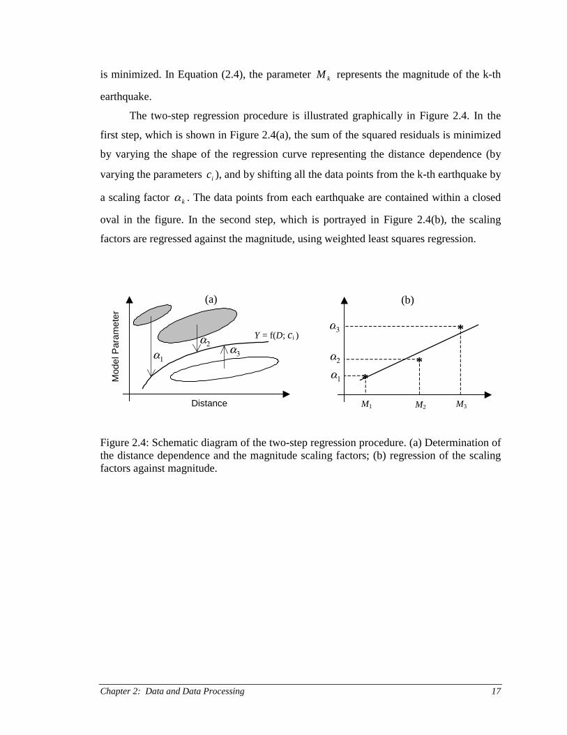
The two-step regression procedure is illustrated graphically in Figure 2.4. In the
first step, which is shown in Figure 2.4(a), the sum of the squared residuals is minimized
by varying the shape of the regression curve representing the distance dependence (by
varying the parameters ic ), and by shifting all the data points from the k-th earthquake by
a scaling factor kα . The data points from each earthquake are contained within a closed
oval in the figure. In the second step, which is portrayed in Figure 2.4(b), the scaling
factors are regressed against the magnitude, using weighted least squares regression.
Y = f(D; ci )
(a)
α2
Mod
el P
aram
eter
Distance M3M2M1
α3
α2
α1
α3α1
*
**
(b)
Figure 2.4: Schematic diagram of the two-step regression procedure. (a) Determination ofthe distance dependence and the magnitude scaling factors; (b) regression of the scalingfactors against magnitude.

Chapter 3: Modeling of Phase Differences: Parametric Method 19
CHAPTER 3MODELING OF PHASE DIFFERENCES:
PARAMETRIC METHOD
In this study, the frequency-dependent characteristics of earthquake accelerograms are
investigated using the discrete Fourier transform. In this chapter, an empirical method for
the modeling of Fourier phase differences is presented. An alternative theoretical method
is presented in the next chapter, and the modeling of the Fourier amplitude spectrum is
discussed in Chapter 5.
In the first section of this chapter, the notational convention for the discrete
Fourier transform is established. In the subsequent sections, an empirical phase difference
distribution model is described, and prediction formulas for the model parameters are
developed using the California ground motion database and the two-step regression
procedure presented in Chapter 2. Finally, the quality of the fitted phase difference
distributions is examined. The statistics on the phase difference distributions that are used
in this chapter are tabulated in Appendix B.
3.1 The Discrete Fourier Transform
For digitally sampled time histories, both the time series, f(tk), and its Fourier transform,
F(ωj), are functions of a discrete argument (time and frequency, respectively). The
discrete Fourier transform is defined here by:
( ) ( ) ( ) 12,,2;exp1 12
2
−−=⋅⋅−⋅= ∑−
−=NNjtitf
NF
N
Nkkjkj ωω (3.1)
and the inverse discrete Fourier transform is given by:
( ) ( ) ( ) 12,,2;exp12
2
−−=⋅⋅⋅= ∑−
−=NNktiFtf
N
Njkjjk ωω (3.2)

Chapter 3: Modeling of Phase Differences: Parametric Method20
where F(ωj) is the discrete Fourier transform evaluated at the j-th circular frequency, ωj:
12,,2;22 −−=⋅⋅=⋅= NNj
tN
j
T
j
dj
∆ππω (3.3)
In Equation (3.3), Td is the total duration of the time series, ∆t is the sampling interval,
and N is the order of the discrete Fourier transform.
The discrete Fourier transform given by Equation (3.1) is a complex function that
can be characterized by its amplitude and phase angle:
( ) ( )jjj iAF Φω ⋅⋅= exp (3.4)
where Aj is the Fourier amplitude corresponding to ωj, and Φj is the phase angle. While
the Fourier amplitudes of earthquake ground acceleration have been studied extensively,
the phase angles have received little or no attention. Frequently, the phase angles are
assumed to be independent of each other and uniformly distributed (e.g. Shinozuka and
Deodatis, 1988). The validity of this independence and uniformity assumption is
examined in the following section.
3.2 Characterization of Fourier Phase Differences
In earthquake ground motion modeling, the Fourier phase angles, Φj, are most frequently
assumed to be independent, both of each other and the Fourier amplitude. In addition, the
phase angles are typically assumed to be uniformly distributed between 0 and 2π or -π
and π. For a stationary Gaussian process, it can be shown that these are valid
assumptions. The objective of this section is to demonstrate that these assumptions are
not justifiable for a typical (nonstationary) ground motion record, and to propose an
alternative model.
Figure 3.1 shows the results of an analysis of a typical recording of horizontal
ground acceleration from a moderate size earthquake. The analysis involves taking a
2048 point discrete Fourier transform and evaluating the phase angles and the phase

Chapter 3: Modeling of Phase Differences: Parametric Method 21
differences, creating histograms of these quantities and plotting them as function of
frequency as well as the Fourier amplitude.
The graphs on the left hand side of Figure 3.1 show the results of the analysis of
the phase angles. Figure 3.1(a) shows a histogram of the phase angles for non-negative
frequencies. The distribution is very close to uniform. In Figure 3.1(c), the phase angles
are plotted versus frequency. The points appear to be uniformly scattered throughout the
entire frequency-phase angle domain. In Figure 3.1(e), the phase angles are plotted as
function of the Fourier amplitude. Once again, no systematic pattern is observed. For a
given amplitude, the phase angles seem to be uniformly distributed between -π and π.
Therefore, one can justify the assumption that the phase angles follow a uniform
distribution. It is, however, a different question whether the phase angles are independent
of each other. That question can be answered by looking at the phase differences.
The right hand side of Figure 3.1 illustrates the results of analyses on the phase
differences. The phase difference is defined as the difference in phase angles of adjacent,
non-negative frequencies:
12,,1,0;1 −=−= + Njjjj ΦΦ∆Φ (3.5)
A histogram of observed phase differences is shown in Figure 3.1(b). The histogram is
clearly non-uniform. It should be noted that before constructing this histogram, the phase
differences are unwrapped. The phase angle domain is [-π, π] and hence the phase
difference domain should be [-2π, 2π]. However, prior to further analyses, a factor of 2π
is subtracted from the phase difference if it exceeds π, and 2π are added to the phase
difference if it is less than -π. Therefore, the unwrapped phase difference domain
becomes [-π, π].
A scatterplot of the phase differences as function of frequency is displayed in
Figure 3.1(d). As can be seen in this figure, the phase difference distribution appears to
be independent of frequency. The independence assumption, however, seems no longer
valid when the phase differences are plotted as function of the Fourier amplitude, as
shown in Figure 3.1(f). While the mean phase difference does not appear to depend on
amplitude, the dispersion around the mean decreases with increasing amplitude.

Chapter 3: Modeling of Phase Differences: Parametric Method22
Figure 3.1: Observed phase angles and phase differences for the east-west component ofthe Santa Cruz record from the 1989 Loma Prieta, California earthquake. (a) Histogramof phase angles; (b) histogram of phase differences; (c) phase angles as function offrequency; (d) phase differences as function of frequency; (e) phase angles as function ofamplitude; (f) phase differences as function of amplitude.

Chapter 3: Modeling of Phase Differences: Parametric Method 23
For a stationary stochastic process, the phase angles and the phase differences are
independent, identically distributed and uniform. As shown in Figure 3.1, this is not the
case for typical earthquake accelerograms. Therefore, the phase differences contain
information on the non-stationarity of the process. By properly modeling this
phenomenon, it is perhaps possible to simulate earthquake accelerograms in the
frequency domain, invert the discrete Fourier transform, and obtain the nonstationary
time series without employing any explicit modulation functions. This hypothesis is
tested in this and the following chapter.
Several researchers have attempted to fit statistical distributions to the phase
differences. Ohsaki (1979) performs statistical analysis on 49 Japanese accelerograms
recorded on rock, and infers that the probability distribution is “normal or normal-like”,
after introducing a proper shift of the phase difference domain to account for the
asymmetry. Kanda et al. (1983) simulate accelerograms using uniform distributions for
the phase differences at different frequency bands. The width of the uniform distribution
decreases with increasing frequency. Similarly, the mean phase difference decreases to
ensure that the higher frequencies, in general, will occur before the lower frequencies in
the simulated time series. Naraoka and Watanabe (1987) simulate accelerograms using a
lognormal distribution for the phase differences. Matsukawa et al. (1987) fit a normal
distribution to the phase differences, after a proper shift, and they find the fit to be “good”
based on a chi-square test. Sigbjörnsson et al. (1994) develop probabilistic seismic hazard
maps by simulating accelerograms using a normal distribution for the phase differences.
To capture the dependence of phase angle differences on Fourier amplitude, the
amplitudes are classified into three categories in this chapter: small, intermediate and
large. Statistical analyses are performed on the phase differences corresponding to each
amplitude category. The 10% largest amplitudes are defined as large, the 55% smallest
are defined as small, and the remaining are intermediate. Several other cut-off fractiles
were examined, but based on analysis of many recorded time histories from different
earthquakes, the two fractiles mentioned above (55% and 90%) yielded the most
consistent results. An attempt was made to use only two Fourier amplitude categories,
small and large, but the simulated accelerograms did not look realistic. In Section 3.4, it
is shown that classifying the Fourier amplitudes into three categories yields sufficiently

Chapter 3: Modeling of Phase Differences: Parametric Method24
good results. Therefore, finer discretization was not pursued. In the next chapter, the
amplitude range is not discretized at all, but a Fourier phase difference distribution is
developed where the parameters are continuous functions of the Fourier amplitude.
Phase difference histograms for an entire time history and for each amplitude
category are displayed in Figure 3.2. The dispersion of the phase differences is
considerably smaller for the large amplitudes than the small ones.
Figure 3.2: Histograms of phase differences for different amplitude categories. The east-west component of the UC Santa Cruz record from the 1989 Loma Prieta, Californiaearthquake.
The distribution fitted to the phase differences should take into account the
circular nature of the phase differences, i.e. the probability density should have the same
value at -π as at +π. The beta distribution appears to be an obvious choice for the large
and the intermediate Fourier amplitudes. It describes the probability distribution of a
bounded random variable, and if both its shape parameters are larger than one, the
probability density function is unimodal and zero at both ends. For the small amplitudes,
however, it is found useful to superimpose a beta on a uniform distribution. To facilitate

Chapter 3: Modeling of Phase Differences: Parametric Method 25
the use of the standardized beta distribution, the phase differences are first shifted from [-
π, π] to [-1.4π, 0.6π] in order to obtain a unimodal distribution, and then the shifted phase
differences are normalized to the interval [0,1].
The probability density function of a beta distributed random variable, X, which is
bounded between zero and one, is given by:
( ) ( )( ) ;10;
,
1 11
≤≤−=−−
xsrB
xxxf
sr
X (3.6)
where r, s > 0 are the shape parameters of the distribution, and the normalizing constant
is given by:
( ) ( )∫ −− −=1
0
11 1, duuusrB sr (3.7)
The cumulative distribution function, which is sometimes referred to as the incomplete
beta function, does not exist in a closed form for arbitrary values of r and s. The mean
and the variance of the random variable X are related to the shape parameters according
to:
( ) ( )122
++⋅+⋅=
+=
srsr
srsr
r
X
X
σ
µ(3.8)
where Xµ is the mean and 2Xσ represents the variance.
An example of the fitted phase difference distributions is shown in Figure 3.3 for
large, intermediate and small Fourier amplitudes. The parameters of the beta distribution
for the different amplitude categories are estimated using the method of moments. The
relative weight of the uniform distribution for small amplitudes is obtained as follows.
First, the interval between zero and one is discretized into ten bins and the number of
observed phase differences within each bin is determined. Then the numbers within the
bins are scaled such that the total area of the histogram equals one. Finally, the relative
weight of the uniform distribution is determined as the height of the smallest bar, after

Chapter 3: Modeling of Phase Differences: Parametric Method26
scaling. In Figure 3.3, the fitted distributions are shown with black dashed lines, while the
observed distributions are shown with gray solid lines.
Figure 3.3: Fitted (dashed lines) and observed (bars, solid lines) conditional phasedifference distributions. The east-west component of the UC Santa Cruz record from the1989 Loma Prieta, California earthquake.

Chapter 3: Modeling of Phase Differences: Parametric Method 27
3.3 Model Parameters
A beta distribution can either be characterized by the mean and the variance of the
random variable, or by the two shape parameters of the distribution. In this study, the
means and the variances are used to define the beta distributions for normalized phase
differences, because the sample means and variances are uncorrelated, while the
estimates of the shape parameters are correlated.
The model of the phase differences described in the previous section requires
seven parameters: the mean normalized phase difference and variance for small,
intermediate, and large Fourier amplitudes, respectively, and the relative weight of the
uniform distribution for small Fourier amplitudes. In this section, the dependency
between the model parameters is examined, and prediction formulas are developed.
Analyses of the ground motion data from California show that the seven phase difference
parameters are not mutually independent. The relationship between the parameters is
illustrated in Figures 3.4, 3.5 and 3.6.
In Figure 3.4(a) the mean normalized phase difference for intermediate Fourier
amplitudes is plotted as a function of the mean phase difference for large amplitudes. A
distinct linear trend is apparent. In Figure 3.4(b), the relationship between the mean phase
difference for small amplitudes and the mean phase difference for large amplitudes is
examined. As observed for the intermediate amplitudes, the mean phase difference for
small amplitudes seems to be linearly related to the mean phase difference for large
amplitudes. According to Figure 3.4, it is sufficient to develop prediction formulas based
on magnitude and distance for the mean normalized phase difference for large Fourier
amplitudes only. Once that has been determined, the mean values for intermediate and
small Fourier amplitudes can easily be estimated using linear regression.
The relationships between the variances of the normalized phase differences are
examined in Figure 3.5. The variance of phase differences for small amplitudes is taken
as the independent variable and plotted on the horizontal axes. In Figures 3.5(a) and
3.5(c) the variance for large Fourier amplitudes is plotted on the vertical axes. In Figures
3.5(b) and 3.5(d) the variance for intermediate Fourier amplitudes is plotted on the
vertical axes. The figures at the top, 3.5(a) and 3.5(b), are in linear space, while the

Chapter 3: Modeling of Phase Differences: Parametric Method28
figures at the bottom, 3.5(c) and 3.5(d), are in logarithmic space. The scatterplots in
Figures 3.5(c) and 3.5(d) reveal a linear trend where the dispersion around a potential
regression line does not appear to depend on the independent variable, i.e. the logarithm
of the variance for small Fourier amplitudes. Hence, the variance of the normalized phase
difference for large and intermediate Fourier amplitudes, respectively, are regressed
against the variance for small amplitudes in logarithmic space.
Figure 3.4: The relationship between average normalized phase differences for theCalifornia ground motion records. (a) Average normalized phase difference forintermediate Fourier amplitudes vs. average normalized phase difference for largeFourier amplitudes; (b) average normalized phase difference for small Fourier amplitudesvs. average normalized phase difference for large Fourier amplitudes.
A scatterplot of the relative weight of the uniform distribution versus the variance
of normalized phase difference for small Fourier amplitudes is shown in Figure 3.6.
Based on the linear trend revealed in this figure, the weight of the uniform distribution is
determined from linear regression on the variance.
It can be concluded from Figures 3.4, 3.5, and 3.6 that information on only two
phase difference parameters, i.e. the mean normalized phase difference for large
amplitudes and the variance of normalized phase difference for small amplitudes, are
generally sufficient to infer the values of the other five parameters. For the remainder of
this report, the mean of the normalized phase difference for large Fourier amplitudes and
the variance of normalized phase difference for small Fourier amplitudes are referred to

Chapter 3: Modeling of Phase Differences: Parametric Method 29
as the fundamental parameters, while the other five parameters are referred to as the
secondary parameters. In the following subsections, the results of the regression analyses
of the phase difference parameters are presented. First, prediction formulas for the
fundamental parameters are developed, followed by regression analyses of the secondary
parameters as function of the fundamental parameters. Prediction formulas are developed
for the fundamental parameters for all sites, as well as different site classes (see
Subsection 2.1.3 for the definition of site classes), while the local site conditions are not
explicitly accounted for in the development of the prediction formulas for the secondary
beta parameters. However, the site conditions are implicitly taken into account, since the
secondary parameters are conditional on the fundamental parameters.
Figure 3.5: The relationship between the variance of normalized phase differences for theCalifornia ground motion records. (a) The variance for large amplitudes vs. the variancefor small amplitudes on a linear scale; (b) the variance for intermediate amplitudes vs. thevariance for small amplitudes on a linear scale; (c) the variance for large amplitudes vs.the variance for small amplitudes on a logarithmic scale; (d) the variance for intermediateamplitudes vs. the variance for small amplitudes on a logarithmic scale.

Chapter 3: Modeling of Phase Differences: Parametric Method30
Figure 3.6: The weight of the uniform distribution as function of the variance ofnormalized phase difference for small amplitudes.
3.3.1 Fundamental Parameters
The fundamental parameters are the mean normalized phase difference for large Fourier
amplitudes and the variance of the normalized phase difference for small amplitudes. The
five secondary beta parameters can all be determined conditional on these two
fundamental parameters, which is done in the following subsection. In this subsection,
the two-step regression procedure described in Section 2.2 is used to obtain prediction
formulas for the fundamental parameters, based on the magnitude of the earthquake and
the source to site distance.
The Mean Normalized Phase Difference for Large Amplitudes
In Figure 3.7, the mean normalized phase difference for large Fourier amplitudes is
plotted as function of distance for two earthquakes; the Mw = 5.9 1987 Whittier Narrows
earthquake, and the Mw = 6.9 1989 Loma Prieta earthquake. Two trends are apparent
from this scatterplot: (i) the mean normalized phase difference decreases with distance,

Chapter 3: Modeling of Phase Differences: Parametric Method 31
and (ii) the mean phase difference for the smaller earthquake tends to be slightly larger
than the mean phase difference for the larger earthquake. Furthermore, the mean seems to
decrease roughly linearly with distance.
Figure 3.7: Mean normalized phase difference for large Fourier amplitudes as function ofdistance, for two different earthquake magnitudes.
With these two observations in mind, the following regression model is fitted to
the data:
( )WML Mc
Dcc ⋅+= 21µ (3.9)
where Lµ is the mean normalized phase difference for large Fourier amplitudes, D is the
distance of the site from the source, and 1c , 2c and ( )WM Mc are regression coefficients.
The coefficients ( )WM Mc are magnitude-dependent scaling factors. In the second step of
the regression procedure, a linear model is fitted to the magnitude scaling factor:
WM Mqqc ⋅+= 21 (3.10)
Here, 1q and 2q are regression coefficients, and WM is the moment magnitude.
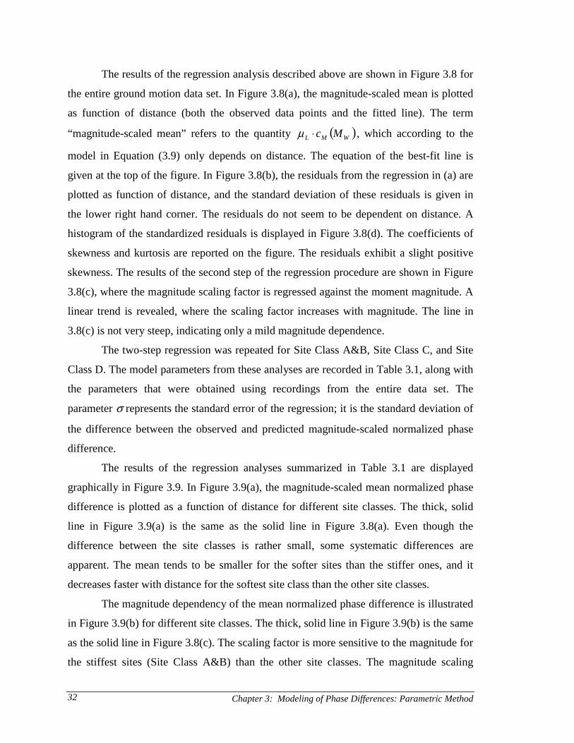
Chapter 3: Modeling of Phase Differences: Parametric Method32
The results of the regression analysis described above are shown in Figure 3.8 for
the entire ground motion data set. In Figure 3.8(a), the magnitude-scaled mean is plotted
as function of distance (both the observed data points and the fitted line). The term
“magnitude-scaled mean” refers to the quantity ( )WML Mc⋅µ , which according to the
model in Equation (3.9) only depends on distance. The equation of the best-fit line is
given at the top of the figure. In Figure 3.8(b), the residuals from the regression in (a) are
plotted as function of distance, and the standard deviation of these residuals is given in
the lower right hand corner. The residuals do not seem to be dependent on distance. A
histogram of the standardized residuals is displayed in Figure 3.8(d). The coefficients of
skewness and kurtosis are reported on the figure. The residuals exhibit a slight positive
skewness. The results of the second step of the regression procedure are shown in Figure
3.8(c), where the magnitude scaling factor is regressed against the moment magnitude. A
linear trend is revealed, where the scaling factor increases with magnitude. The line in
3.8(c) is not very steep, indicating only a mild magnitude dependence.
The two-step regression was repeated for Site Class A&B, Site Class C, and Site
Class D. The model parameters from these analyses are recorded in Table 3.1, along with
the parameters that were obtained using recordings from the entire data set. The
parameter σ represents the standard error of the regression; it is the standard deviation of
the difference between the observed and predicted magnitude-scaled normalized phase
difference.
The results of the regression analyses summarized in Table 3.1 are displayed
graphically in Figure 3.9. In Figure 3.9(a), the magnitude-scaled mean normalized phase
difference is plotted as a function of distance for different site classes. The thick, solid
line in Figure 3.9(a) is the same as the solid line in Figure 3.8(a). Even though the
difference between the site classes is rather small, some systematic differences are
apparent. The mean tends to be smaller for the softer sites than the stiffer ones, and it
decreases faster with distance for the softest site class than the other site classes.
The magnitude dependency of the mean normalized phase difference is illustrated
in Figure 3.9(b) for different site classes. The thick, solid line in Figure 3.9(b) is the same
as the solid line in Figure 3.8(c). The scaling factor is more sensitive to the magnitude for
the stiffest sites (Site Class A&B) than the other site classes. The magnitude scaling

Chapter 3: Modeling of Phase Differences: Parametric Method 33
factor for Site Class C is practically the same as the magnitude scaling factor for Site
Class D.
Figure 3.8: Results of a two step regression analysis for the mean normalized phasedifference for large Fourier amplitudes and all site classes. (a) The distance dependenceof the magnitude-scaled mean; (b) residuals from (a) as function of distance; (c) themagnitude dependent scaling factor; (d) histogram of the standardized residuals from (a).
Table 3.1: Regression results for Lµ .Data Set
1c 2c 1q 2q σ
All Sites 0.56 -0.0023 0.41 0.092 0.0485
Site Class A&B 0.60 -0.0023 -0.67 0.259 0.0386
Site Class C 0.55 -0.0021 0.40 0.094 0.0560
Site Class D 0.55 -0.0027 0.51 0.077 0.0397
Model:W
L Mqq
Dcc
⋅+⋅+=
21
21µ
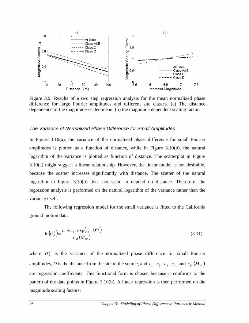
Chapter 3: Modeling of Phase Differences: Parametric Method34
Figure 3.9: Results of a two step regression analysis for the mean normalized phasedifference for large Fourier amplitudes and different site classes. (a) The distancedependence of the magnitude-scaled mean; (b) the magnitude dependent scaling factor.
The Variance of Normalized Phase Difference for Small Amplitudes
In Figure 3.10(a), the variance of the normalized phase difference for small Fourier
amplitudes is plotted as a function of distance, while in Figure 3.10(b), the natural
logarithm of the variance is plotted as function of distance. The scatterplot in Figure
3.10(a) might suggest a linear relationship. However, the linear model is not desirable,
because the scatter increases significantly with distance. The scatter of the natural
logarithm in Figure 3.10(b) does not seem to depend on distance. Therefore, the
regression analysis is performed on the natural logarithm of the variance rather than the
variance itself.
The following regression model for the small variance is fitted to the California
ground motion data:
( ) ( )( )WM
c
S Mc
Dccc 43212 exp
ln⋅⋅+=σ (3.11)
where 2Sσ is the variance of the normalized phase difference for small Fourier
amplitudes, D is the distance from the site to the source, and 1c , 2c , 3c , 4c , and ( )WM Mc
are regression coefficients. This functional form is chosen because it conforms to the
pattern of the data points in Figure 3.10(b). A linear regression is then performed on the
magnitude scaling factors:

Chapter 3: Modeling of Phase Differences: Parametric Method 35
WM Mqqc ⋅+= 21 (3.12)
where, 1q and 2q are regression coefficients, and WM is the moment magnitude of the
earthquake.
Figure 3.10: Variance of normalized phase difference for small Fourier amplitudes asfunction of distance. (a) The variance versus distance; (b) the natural logarithm of thevariance as function of distance.
The results of the two-step regression analysis for the variance using the entire
ground motion data set are shown in Figure 3.11. In Figure 3.11(a), the magnitude-scaled
natural logarithm is plotted as function of distance; both the observed data points and the
fitted curve. The equation of the best-fit curve is given at the top of the figure. In Figure
3.11(b), the residuals from the regression in (a) are plotted as function of distance, and
the standard deviation of these residuals is given in the lower right hand corner. The
residuals do not seem to be dependent on distance. A histogram of the standardized
residuals is displayed in Figure 3.11(d). The coefficients of skewness and kurtosis are
reported on the figure. The residuals exhibit a slight positive skewness. The results of the
second step of the regression procedure are shown in Figure 3.11(c), where the
magnitude scaling factor is regressed against the moment magnitude. The scaling factor –
and hence, the variance – does not appear to depend on magnitude.
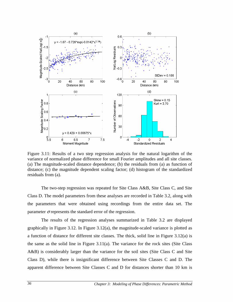
Chapter 3: Modeling of Phase Differences: Parametric Method36
Figure 3.11: Results of a two step regression analysis for the natural logarithm of thevariance of normalized phase difference for small Fourier amplitudes and all site classes.(a) The magnitude-scaled distance dependence; (b) the residuals from (a) as function ofdistance; (c) the magnitude dependent scaling factor; (d) histogram of the standardizedresiduals from (a).
The two-step regression was repeated for Site Class A&B, Site Class C, and Site
Class D. The model parameters from these analyses are recorded in Table 3.2, along with
the parameters that were obtained using recordings from the entire data set. The
parameter σ represents the standard error of the regression.
The results of the regression analyses summarized in Table 3.2 are displayed
graphically in Figure 3.12. In Figure 3.12(a), the magnitude-scaled variance is plotted as
a function of distance for different site classes. The thick, solid line in Figure 3.12(a) is
the same as the solid line in Figure 3.11(a). The variance for the rock sites (Site Class
A&B) is considerably larger than the variance for the soil sites (Site Class C and Site
Class D), while there is insignificant difference between Site Classes C and D. The
apparent difference between Site Classes C and D for distances shorter than 10 km is

Chapter 3: Modeling of Phase Differences: Parametric Method 37
inconsequential, because there are very few data points to anchor the curves at very short
distances.
The magnitude dependency of the variance is illustrated in Figure 3.12(b) for
different site classes. The thick, solid line in Figure 3.12(b) is the same as the solid line in
Figure 3.11(c). The variance does not seem to depend on the magnitude for the softer
sites (Site Class C and Site Class D), and only mildly so for the rock sites.
To predict the value of the variance of normalized phase difference for small
Fourier amplitudes, it is recommended to use Equations (3.11) and (3.12) with the
parameters corresponding to Site Class A&B from Table 3.2 for rock sites, and the
parameters corresponding to Site Class D from Table 3.2 for all non-rock sites.
Table 3.2: Regression results for 2Sσ .
Data Set1c 2c 3c 4c 1q 2q σ
All Sites -1.67 -0.726 -0.0142 1.14 0.43 0.009 0.168
Site Class A&B -1.46 -0.528 -0.0150 1.23 0.14 0.054 0.066
Site Class C -2.10 -0.973 -0.0555 1.14 0.47 0.002 0.191
Site Class D -2.04 -0.476 -0.0039 1.74 0.51 -0.003 0.176
Model: ( ) ( )W
c
S Mqq
Dccc
⋅+⋅⋅+=
21
32124exp
ln σ
Figure 3.12: Results of a two step regression analysis for the variance of normalizedphase difference for small Fourier amplitudes and different site classes. (a) The distancedependence of the magnitude-scaled variance; (b) the magnitude dependent scalingfactor.

Chapter 3: Modeling of Phase Differences: Parametric Method38
3.3.2 Secondary Parameters
Five more parameters, in addition to the fundamental parameters, are needed to fully
define the Fourier phase difference distributions. These are:
1. The mean normalized phase difference for intermediate Fourier amplitudes,
2. the mean normalized phase difference for small Fourier amplitudes,
3. the variance of normalized phase difference for intermediate Fourier amplitudes,
4. the variance of normalized phase difference for large Fourier amplitudes, and,
5. the weight of the uniform distribution in the probability distribution of normalized
phase difference for small Fourier amplitudes.
In this subsection, the first two parameters are regressed versus the mean normalized
phase difference for large Fourier amplitudes, and the last three are regressed on the
variance of normalized phase difference for small Fourier amplitudes.
The Mean Normalized Phase Difference for Intermediate and Small Amplitudes
The results of the regression analyses of the mean normalized phase difference for
intermediate and small Fourier amplitudes versus the mean for large amplitudes are
displayed in Figure 3.13. The results for the intermediate amplitudes are depicted in the
left column and the results for the small amplitudes are in the right column. The plots at
the top, (a) and (b), show the fitted lines, obtained through linear least squares regression,
superimposed on the observed data points. The equation of the best line is also given in
the upper right hand corner of each plot. The plots in the middle, (c) and (d), show how
the residuals depend on the independent variable (the mean normalized phase difference
for large Fourier amplitudes) and the standard deviation of the residuals is given in the
lower right hand corner. In neither case is there an obvious trend in the residuals, which is
as desired. At the bottom of Figure 3.13, (e) and (f), there are histograms of the
standardized residuals; i.e. zero mean, unit standard deviation. The numbers reported on
the graphs are the coefficients of skewness and kurtosis. In both cases, the residuals
exhibit a positive skewness and kurtosis slightly larger than the kurtosis for a normal
distribution of 3.0.

Chapter 3: Modeling of Phase Differences: Parametric Method 39
Figure 3.13: Regression results for mean phase differences. (a) Intermediate amplitudesvs. large amplitudes; (b) small amplitudes vs. large amplitudes; (c) residuals from theregression in (a); (d) residuals from the regression in (b); (e) histogram of standardizedresiduals from the regression in (a); (f) histogram of standardized residuals from theregression in (b).

Chapter 3: Modeling of Phase Differences: Parametric Method40
The Variance of Normalized Phase Difference for Intermediate Amplitudes
Figure 3.14 displays the results from the regression analysis of the variance of normalized
phase difference for intermediate Fourier amplitudes versus the variance for small
amplitudes. In part (a), the best line is superimposed on the observed data points, in
natural logarithm space. The equation of the best line is given in the lower right hand
corner. The residuals from the linear regression are plotted in part (b), as function of the
independent variable. The standard deviation is shown in the lower right hand corner. No
trend is apparent from this plot. In part (c), the data points and the best line fit from (a)
have been transformed into the original, linear space. A histogram of the standardized
residuals from the linear regression is showed in part (d). The coefficient of skewness is –
0.80, which implies a skewness to the left. The coefficient of kurtosis is 4.14,
considerably higher than the value of 3 for a normal distribution.
Figure 3.14: Results of regression analysis of variance of normalized phase difference forintermediate amplitudes vs. variance of normalized phase difference for smallamplitudes. (a) Linear regression in natural logarithm space; (b) residuals of theregression in (a); (c) the regression in (a) transformed into linear space; (d) histogram ofstandardized residuals from (a).
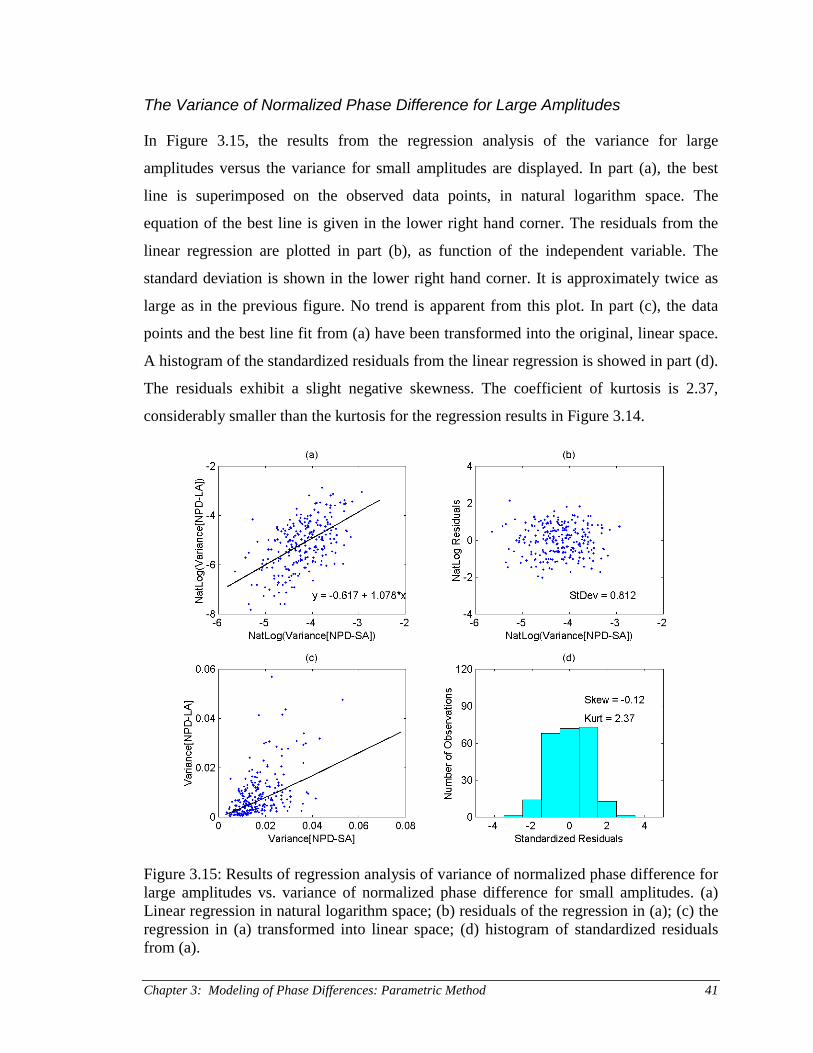
Chapter 3: Modeling of Phase Differences: Parametric Method 41
The Variance of Normalized Phase Difference for Large Amplitudes
In Figure 3.15, the results from the regression analysis of the variance for large
amplitudes versus the variance for small amplitudes are displayed. In part (a), the best
line is superimposed on the observed data points, in natural logarithm space. The
equation of the best line is given in the lower right hand corner. The residuals from the
linear regression are plotted in part (b), as function of the independent variable. The
standard deviation is shown in the lower right hand corner. It is approximately twice as
large as in the previous figure. No trend is apparent from this plot. In part (c), the data
points and the best line fit from (a) have been transformed into the original, linear space.
A histogram of the standardized residuals from the linear regression is showed in part (d).
The residuals exhibit a slight negative skewness. The coefficient of kurtosis is 2.37,
considerably smaller than the kurtosis for the regression results in Figure 3.14.
Figure 3.15: Results of regression analysis of variance of normalized phase difference forlarge amplitudes vs. variance of normalized phase difference for small amplitudes. (a)Linear regression in natural logarithm space; (b) residuals of the regression in (a); (c) theregression in (a) transformed into linear space; (d) histogram of standardized residualsfrom (a).

Chapter 3: Modeling of Phase Differences: Parametric Method42
The Weight of the Uniform Distribution
The last beta parameter is the weight of the uniform distribution for small Fourier
amplitudes. As suggested by the scatterplot in Figure 3.6, a linear regression is performed
on the weight of the uniform distribution as function of the variance for small amplitudes.
The results of such regression analyses are summarized in Figure 3.16. In Figure 3.16(a),
the fitted line is superimposed on the observed data points. The equation of the regression
line is displayed in the lower right hand corner of the figure. The residuals from the linear
regression are plotted in Figure 3.16(b) as function of the independent variable, the
variance of normalized phase difference for small Fourier amplitudes. For small values of
the independent variable, the absolute value of the residuals tends to increase as the
independent variable increases. This is due to the fact that up to a certain threshold value
of the independent variable, there are observations of the dependent variable around its
lower limit. The standardized residuals are plotted in Figure 3.16(c), and a histogram of
the standardized residuals is displayed in Figure 3.16(d). The coefficients of skewness
and kurtosis for the residuals are reported in Figure 3.16(d). The residuals display a
considerable positive skewness, and the coefficient of kurtosis is 3.56.
The inhomogeneous distribution of the residuals with respect to the independent
variable implies that it would be more desirable to select the weight of the uniform
distribution as the independent variable and the variance of the normalized phase
difference for small amplitudes as the dependent variable. However, the other secondary
parameters, i.e. the variances of normalized phase difference for intermediate and large
Fourier amplitudes, respectively, showed much better correlation with the variance than
with the weight of the uniform distribution for small Fourier amplitudes. Therefore, it
was decided to regress the weight of the uniform distribution on the variance, rather than
vice versa.

Chapter 3: Modeling of Phase Differences: Parametric Method 43
Figure 3.16: Results of regression analysis for the weight of the uniform distributionversus the variance of normalized phase difference for small Fourier amplitudes. (a)Linear regression; (b) residuals; (c) standardized residuals; (d) histogram of standardizedresiduals.
3.4 Model Validation
In Section 3.2 it was shown qualitatively that conditional beta distributions could be used
to model the normalized Fourier phase differences – at least in that particular example.
This single example does not, however, validate the beta model in general. For general
validation, more exhaustive, systematic and quantitative tests of the method are needed.
In this section, several tests are performed to estimate how well the assumed
model, i.e. the conditional beta distributions for normalized Fourier phase differences, fit
real observations. Four different quality tests are performed: statistical goodness of fit
tests for the distribution functions, and three different tests where the characteristics of
simulated accelerograms are compared to the corresponding characteristics of recorded
Chapter 3: Modeling of Phase Differences: Parametric Method44
accelerograms. These include comparisons of peak ground acceleration values, linear
response spectra, and the temporal distribution of the energy content. All four tests are
performed on the entire ground motion database that was used to develop the prediction
formulas for the beta parameters.
3.4.1 Phase Difference Distributions
The Kolmogorov-Smirnov goodness of fit test is used to estimate the statistical goodness
of fit of the conditional beta distributions. The statistic used to estimate how well an
assumed probability distribution fits observed data is the maximum of the absolute
difference between the assumed (or fitted) and observed (or empirical) cumulative
distribution function:
( ) ( )xFxFS Xnx
n −=all
max (3.13)
Here, nS is the Kolmogorov-Smirnov statistic, ( )xFX is the assumed cumulative
distribution function, and ( )xFn is the empirical cumulative distribution function. The
empirical cumulative distribution is given by:
( ) njn
jxF jn ,,2,1; == (3.14)
where jx is the j-th smallest sample and n is the number of observations; the sample size.
The assumed probability distribution is rejected if the test statistic is larger than a certain
critical value, i.e. if
reject, ⇒> crnn SS (3.15)
For large samples (for example, n > 80), the critical value can be approximated by
(Lindgren, 1976):
( )n
S crn 2
2ln,
α−= (3.16)

Chapter 3: Modeling of Phase Differences: Parametric Method 45
where α is the significance level of the test. The significance level is equal to the
probability of rejecting the assumed distribution, when it is the true distribution. It is
usually chosen to be a small number, very often of the order of 0.01 to 0.10.
A discrete 2048 points Fourier transform yields 1024 unique observations of
phase difference (see Equation 3.5). As described in Section 3.2, fifty-five percent, or
563, belong to the small Fourier amplitudes, there are 358 observations in the
intermediate category, and 103 belong to the large Fourier amplitudes category. The
large-sample-approximation of Equation (3.16) can therefore be used for all three
amplitude categories. The critical values for the Kolmogorov-Smirnov statistic,
calculated according to Equation (3.16), are given in Table 3.3, for each Fourier
amplitude category and three different significance levels.
Table 3.3: Critical values of the Kolmogorov-Smirnov statistic for normalized phasedifference distributions.
SmallAmplitudes
(n = 563)
IntermediateAmplitudes
(n = 358)
LargeAmplitudes
(n = 103)1% Significance 0.0686 0.0860 0.1604
5% Significance 0.0572 0.0718 0.1338
10% Significance 0.0516 0.0647 0.1206
Figure 3.17 shows examples of fitted (dashed lines) and recorded (solid lines)
distributions for the normalized phase difference. The maximum difference between the
two cumulative distribution functions for small Fourier amplitudes is 0.0659. Therefore,
the fitted distribution is rejected at the 5% significance level, but not at the 1%
significance level. For intermediate amplitudes, the maximum difference between the
recorded and the fitted phase difference distributions is 0.1487, which means, that the
fitted distribution is rejected at the 1% significance level. The maximum difference
between the two phase difference distribution functions for large Fourier amplitudes is
0.0835. This value is smaller than all the values in the right most column of Table 3.3, so
the fitted distribution is not rejected at any of the three significance levels.

Chapter 3: Modeling of Phase Differences: Parametric Method46
Figure 3.17: Comparison of observed phase difference distributions (solid lines) andfitted distributions (dashed lines) for small, intermediate and large Fourier amplitudes.The east-west component of the UC Santa Cruz record from the 1989 Loma Prieta,California earthquake.
The statistical goodness of fit results described above are representative for the
earthquake ground motion database assembled in this study. In more than 80% of the
cases, the fitted distributions cannot be rejected at the 10% significance level, and in half
of the remaining cases, the fitted distribution is only rejected for one out of three Fourier
amplitude categories. In fewer than 5% of the cases, a fitted distribution is rejected at the
5% significance level.
In general, the statistical goodness of fit of the beta distributions for normalized
phase differences is satisfactory, as measured by the Kolmogorov-Smirnov test. It is of
more interest, however, whether the accelerograms simulated using these beta
distributions, adequately reproduce the relevant characteristics of recorded
accelerograms. In the following subsection, the attributes of simulated accelerograms are
compared to the corresponding attributes of recorded accelerograms.
3.4.2 Accelerograms
In the preceding subsection, the assumed and observed probability distributions for
normalized phase difference were compared. In this subsection, the characteristics of
simulated accelerograms, using the assumed phase difference distributions, are compared
with the corresponding characteristics of recorded accelerograms. Three different
characteristics are compared: peak values, elastic response spectra, and evolutionary
behavior.

Chapter 3: Modeling of Phase Differences: Parametric Method 47
Peak Ground Acceleration
Figure 3.18 shows an example of a recorded accelerogram, followed by two examples of
simulated accelerograms. The peak ground acceleration (PGA) of the recorded
accelerogram is 0.41g. The mean PGA from ten simulations is 0.46g, and the standard
deviation of the PGA is 0.05g.
Figure 3.18: A recorded time history compared to two examples of simulated timehistories using conditional beta distributions for Fourier phase differences. The east-westcomponent of the UC Santa Cruz record from the 1989 Loma Prieta, Californiaearthquake.
The results displayed in Figure 3.18 are very typical. In over 75% of the cases, the
recorded PGA was within one standard deviation of the mean PGA from ten simulations,
and in all the other cases, the recorded PGA was within two standard deviations of the
mean.

Chapter 3: Modeling of Phase Differences: Parametric Method48
Elastic Response Spectrum
The elastic response spectra are compared in Figure 3.19. The solid line represents the
elastic pseudo acceleration response spectrum of the recorded ground motion, assuming a
damping factor equal to 5% of critical damping. The dashed lines in Figure 3.19 represent
the response spectra of ten simulated acceleration time histories. For all natural periods
depicted in the figure (from 0.1 seconds to 2 seconds), the response spectra of the
simulated time histories envelope the response spectrum of the recorded time history. The
results in Figure 3.19 are representative of the entire ground motion data set.
Figure 3.19: Elastic pseudo acceleration response spectra (5% damping). Solid line: theresponse spectrum of the east-west component of the UC Santa Cruz record from the1989 Loma Prieta, California earthquake; dashed lines: ten simulations using conditionalbeta distributions for Fourier phase differences.
Cumulative Normalized Arias Intensity
Oftentimes, the temporal distribution of the energy content has a great effect on the
response of a structure that is affected by earthquake ground motion. The last
characteristic included in this comparison is the evolutionary behavior of the

Chapter 3: Modeling of Phase Differences: Parametric Method 49
accelerograms. In this study, the evolutionary behavior is quantified in terms of the
cumulative normalized Arias intensity (Arias, 1970):
( )( )( ) dT
t
Ttda
datNI
d≤≤=
∫∫
0;
0
2
0
2
ττ
ττ(3.17)
where NI(t) is the normalized Arias intensity at time t, a(τ) is the value of the acceleration
time history at time τ, and dT is the total duration of the accelerogram.
In Figure 3.20, the cumulative normalized Arias intensities from ten simulations
are compared to the cumulative normalized Arias intensity of a recorded accelerogram. In
general, the simulated accelerograms capture well the evolutionary characteristics of the
recorded accelerogram. However, the energy release of the simulated accelerograms
tends to be a bit smoother than the energy release of the recorded accelerograms. The
cumulative normalized Arias intensity curves for the simulated time histories are not as
flat towards the beginning as the curve for the recorded time history.
Figure 3.20: Cumulative normalized Arias intensity. Solid line: the cumulative Ariasintensity of the east west component of the UC Santa Cruz record from the 1989 LomaPrieta, California earthquake; dashed lines: ten simulations using conditional betadistributions for Fourier phase differences.

Chapter 3: Modeling of Phase Differences: Parametric Method50
3.5 Summary of Conditional Beta Distributions
In this chapter, it is shown that the Fourier phase angles of digital earthquake
accelerograms are uniformly distributed, but not independent of each other. The
dependency is captured through modeling of the phase differences, conditional on the
Fourier amplitude. An empirical approach is developed, where the phase differences are
modeled by a combination of beta and uniform distributions, for three different Fourier
amplitude categories.
Using the empirical method developed in this chapter, seven parameters are
necessary to completely define the phase difference distribution. These include the mean
and variance of the normalized phase difference for small, intermediate and large Fourier
amplitudes, respectively, and the relative weight of the uniform distribution for small
Fourier amplitudes. These seven parameters are not independent of each other. Two of
them, the mean corresponding to large Fourier amplitudes and the variance for small
amplitudes, are shown to be fundamental, and the other five, secondary parameters can be
derived from one of the two fundamental parameters.
The California ground motion database is used to develop prediction formulas for
the beta parameters. The results of the regression analyses are summarized below. The
parameter D is the shortest distance from the site to the surface projection of the
seismogenic rupture in kilometers, and WM is the moment magnitude of the earthquake.
Two of the seven model parameters are shown to be fundamental for the
characterization of the Fourier phase differences: The mean normalized phase difference
for large Fourier amplitudes, Lµ , and the variance of normalized phase difference for
small Fourier amplitudes, 2Sσ . For an unknown site classification, the mean normalized
phase difference for large Fourier amplitudes can be estimated using:
1.75.8km,100;092.041.0
0023.056.0 ≤≤≤⋅+⋅−= W
WL MD
M
Dµ
For Site Class A&B, the mean can be calculated according to:

Chapter 3: Modeling of Phase Differences: Parametric Method 51
1.75.8km,100;209.054.0
0023.060.0 ≤≤≤⋅+−⋅−= W
WL MD
M
Dµ
For Site Class C the mean is given by:
1.75.8km,100;087.037.0
0021.055.0 ≤≤≤⋅+⋅−= W
WL MD
M
Dµ
Finally, for Site Class D, the mean is:
1.75.8km,100;077.051.0
0027.055.0 ≤≤≤⋅+⋅−= W
WL MD
M
Dµ
The variance of the normalized phase difference for small Fourier amplitudes and
an unknown site class can be estimated according to:
( ) ( )1.75.8km,100;
009.043.0
0142.0exp726.067.1ln
14.12 ≤≤≤
⋅+⋅−⋅−−= W
WS MD
M
Dσ
For Site Class A&B the variance can be calculated using:
( ) ( )1.75.8km,100;
054.014.0
0150.0exp528.046.1ln
23.12 ≤≤≤
⋅+⋅−⋅−−= W
WS MD
M
Dσ
For Site Classes C and D the variance can be computed using:
( ) ( )1.75.8km,100;
003.051.0
0039.0exp476.004.2ln
74.12 ≤≤≤
⋅−⋅−⋅−−= W
WS MD
M
Dσ
Each of the five secondary parameters is inferred from one of the two
fundamental parameters. The local site conditions are not accounted for explicitly, but
they are considered implicitly, because the fundamental parameters depend on the site
classification. The mean normalized phase difference for intermediate Fourier amplitudes
is computed from the mean for large amplitudes:

Chapter 3: Modeling of Phase Differences: Parametric Method52
LI µµ ⋅+= 81.011.0
The mean normalized phase difference for small Fourier amplitudes is computed from the
mean for large amplitudes according to:
LS µµ ⋅+= 69.020.0
The variance of normalized phase difference for intermediate Fourier amplitudes is
computed from the variance for small amplitudes:
( ) ( ) 549.0ln897.0ln 22 −⋅= SI σσ
The variance of normalized phase difference for large Fourier amplitudes is computed
from the variance for small amplitudes:
( ) ( ) 617.0ln078.1ln 22 −⋅= SL σσ
The weight of the uniform distribution, wu, is determined from the variance of
normalized phase difference for small Fourier amplitudes:
−⋅
≤=
otherwise;068.00.15
004533.0;02
2
S
Swuσσ
The Fourier phase difference model is validated through extensive statistical
goodness of fit tests, as well as comparison of certain characteristics of the simulated and
recorded accelerograms. These characteristics are: (i) the peak ground acceleration, (ii)
the 5% damped elastic response spectrum, and (iii) the evolutionary behavior as
quantified by the cumulative normalized Arias intensity.

Chapter 4: Modeling of Phase Differences: Method of Envelopes 53
CHAPTER 4MODELING OF PHASE DIFFERENCES:
METHOD OF ENVELOPES
An empirical method for the modeling of Fourier phase differences of earthquake
accelerograms was presented in Chapter 3, where the Fourier amplitude domain was
discretized into three categories and one model was fitted to the phase differences
belonging to each amplitude category. In this chapter, a theoretical approach is presented,
where a normal (Gaussian) distribution with amplitude-dependent parameters is used to
model the phase difference distribution.
The conditional Fourier phase difference model presented in this chapter gives a
theoretical basis for the empirical, parametric phase difference model presented in
Chapter 3. A major virtue of this theoretical model is its reduced number of parameters,
as compared to the parametric model, and their physical meaning. The conditional phase
difference distribution requires only two parameters, a mean time τ representing the
time-centroid of the energy release, and a duration parameter T∆ , which is a measure of
how narrowly the energy release is focused in time.
The modeling approach presented in this chapter utilizes the method of envelopes
for time-varying functions. The Hilbert transform and its properties are central to the
method of envelopes. Therefore, the Hilbert transform is introduced in the first section of
this chapter, followed by a section on the method of envelopes. Then, an analogy
proposed by Nigam (1982) is built upon, yielding a method of envelopes for frequency-
varying functions, and a model for the simulation of acceleration time histories is
presented. Finally, prediction formulas are developed for the model parameters, based on
the California ground motion database described in Chapter 2. The statistics on the phase
difference distributions that are used in this chapter are tabulated in Appendix C.

Chapter 4: Modeling of Phase Differences: Method of Envelopes54
4.1 The Hilbert Transform
The Hilbert transform of the function f(t) is defined as:
( )[ ] ( ) τττ
πd
t
ftfHi ∫
∞
∞− −= 1
(4.1)
where Hi[f(t)] is the Hilbert transform. Two important attributes of the Hilbert transform
can be deducted from its definition: (i) the Hilbert transform of a real valued function is
itself a real valued function, and (ii) the Hilbert transform and the original function are
orthogonal to each other – i.e. they are π/2 out of phase. For example, the Hilbert
transform of a cosine function is a sine function:
( )[ ] ( )ttHi sincos = (4.2)
Assume that the function f(t) is a real valued function. Define a complex valued
function, g(t), such that f(t) forms its real part and its Hilbert transform forms the
imaginary part:
( ) ( ) ( )[ ]tfHiitftg ⋅+= (4.3)
The function g(t), sometimes referred to as the analytic signal corresponding to f(t), can
be equivalently written as:
( ) ( ) ( )( )titCtg Θ⋅⋅= exp (4.4)
where the magnitude of C(t) is defined as the envelope function of g(t), and (t) is a time
dependent phase angle. The time derivative of the phase angle is often referred to as the
instantaneous frequency. These terms are helpful when dealing with the method of
envelopes.

Chapter 4: Modeling of Phase Differences: Method of Envelopes 55
4.2 Envelopes of Time-Varying Functions
Consider the analytic signal U(t), which can be represented as:
( ) ( ) ( )tXitXtU
⋅+= (4.5)
where ( )tX
is the Hilbert transform of the Gaussian, stationary process X(t):
( ) ( ) ( )[ ]ttCtX Θcos⋅= (4.6)
( ) ( ) ( )[ ]ttCtX Θsin⋅=
(4.7)
The amplitude at time t, C(t), and the phase angle at time t, Θ(t), are uncorrelated random
variables. The amplitudes, C(t), follow a Rayleigh distribution, given by:
( ) 0;2
exp2
2
2≥
−= c
cccf
XXC σσ
(4.8)
where 2Xσ is the variance of X(t). The phase angles are uniformly distributed:
( ) πθπ
θΘ 20;2
1 ≤≤=f (4.9)
If the instantaneous frequency is defined as:
ΘΘΩ ==dt
d(4.10)
i.e. the instantaneous frequency is defined as the rate of change of the phase angle
process Θ(t), the joint probability density of amplitude and frequency is given by
(Sveshnikov, 1968; Winterstein, 1991):

Chapter 4: Modeling of Phase Differences: Method of Envelopes56
( ) ∞<<∞−≥
−+−= ω
∆ωωω
σπ∆ωσωΩ ;0;1
2exp
2,
2
2
2
3
2
ccc
cfXX
C (4.11)
where the mean frequency is given by:
0
1
λλω = (4.12)
and nλ is the n-th spectral moment about the origin:
( ) 2,1,0;0
== ∫∞
ndS Xn
n ωωωλ (4.13)
Here, SX(ω) is the power spectral density of X(t). The parameter ∆ is a unitless parameter
reflecting the spectral bandwidth. It is given by:
( ) 112
01
0221
20 −=−=λλλλ
λλλ∆ (4.14)
The spectral bandwidth parameter ∆ depends on the two spectral moment ratios, λ1/λ0
and λ2/λ0, and it approaches zero as the bandwidth of the power spectral density
decreases.
The joint density of amplitude and frequency as defined in Equation (4.11), can
be factored into the product of the conditional density of the frequency given the
amplitude, and the amplitude density:
( ) ( ) ( )cfcfcf CCC ⋅= ωω ΩΩ , (4.15)
Substituting Equation (4.8) for the amplitude density, one obtains:
( ) ∞<<∞−
−−= ωσ∆ωωω
σ∆ωπωΩ ;
2
1exp
2
12
cccf
XX
C (4.16)

Chapter 4: Modeling of Phase Differences: Method of Envelopes 57
Hence, the conditional distribution of the instantaneous frequency given the amplitude is
Gaussian, with mean
[ ]0
1EλλωΩ ==c (4.17)
and variance
[ ]2
/Var
⋅=Xc
cσ∆ωΩ (4.18)
The mean frequency in Equation (4.17) is independent of the amplitude, while the
standard deviation in Equation (4.18) is inversely proportional to the normalized
amplitude, Xc σ . The dependency of the mean frequency and the mean +/- one standard
deviation on amplitude are illustrated in Figure 4.1.
Figure 4.1: Conditional mean and mean +/- one standard deviation of normalizedinstantaneous frequency, ωω , as function of normalized amplitude, Xc σ . The spectralbandwidth parameter assumed here is 1=∆ .

Chapter 4: Modeling of Phase Differences: Method of Envelopes58
The method of envelopes, as presented above, is used to describe narrow band,
stochastic processes in the time domain. In the following section, the method of
envelopes is applied to a stochastic process in the frequency domain.
4.3 Envelopes of Frequency-Varying Functions
Nigam (1982) suggests applying the method of envelopes to a stochastic process where
frequency is the indexing parameter, rather than time. A stationary process in the time
domain is then analogous to a white process in the frequency domain, the power spectral
density is replaced by the intensity function, and the spectral moments become intensity
moments (see Table 4.1).
Assume that the process Z(ω) is an analytic signal in the frequency domain:
( ) ( ) ( )ωωω YiYZ ˆ⋅+= (4.19)
where Y(ω) is a zero-mean, stationary process in the frequency domain (a “white”
process):
( ) ( ) ( )[ ]ωΦωω sin⋅= AY (4.20)
Here, A(ω) is the Rayleigh distributed amplitude of Z(ω), and Φ(ω) is the uniformly
distributed phase angle. The process Z(ω) can be interpreted as the Fourier transform of
an amplitude modulated stationary Gaussian noise process in the time domain:
( ) ( ) ( )dttitWZ ∫∞
∞−−⋅= ω
πω exp
2
1(4.21)
where
( ) ( ) ( )tXttW ⋅=η (4.22)
and X(t) is a stationary, zero mean, real valued Gaussian noise process with power
spectral density S0. The function η(t) is a deterministic amplitude modulation function, or

Chapter 4: Modeling of Phase Differences: Method of Envelopes 59
an envelope function. The envelope function is non-negative; positive inside the duration
interval of the process W(t), but zero outside of it:
( ) ( )( ) otherwise;0
,0;0
=∈>
t
Ttt d
ηη
(4.23)
Figure 4.2 illustrates the processes X(t) and W(t), and the function η(t).
Figure 4.2: An example of an amplitude modulated process. (a) The stationary noiseprocess, ( )tX ; (b) the amplitude modulation function, ( )tη ; (c) the modulated process,
( )tW .
The process W(t) is zero mean, Gaussian, real valued and causal, with the
autocorrelation function:
( ) ( ) ( )[ ] ( ) ( ) ( ) ≤≤−⋅⋅
=⋅=otherwise;0
,0;E, 211221
2121dX
W
TttttRtttWtWttR
ηη(4.24)
where RX(t2 – t1) is the autocorrelation function of X(t). The autocorrelation function of
the complex valued, zero mean, Gaussian process Z(ω) is given by:

Chapter 4: Modeling of Phase Differences: Method of Envelopes60
( ) ( ) ( )[ ]
( ) ( ) ( ) ( ) ( ) ∫ ∫∞
∞−
∞
∞−−−⋅−⋅⋅=
⋅=
21112212212
2121
exp2
1
*E,
dtdtttittRtt
ZZR
X
Z
ωωηηπ
ωωωω(4.25)
Since X(t) is a Gaussian noise process, with the power spectral density S0, its
autocorrelation function is given by:
( ) ( )12012 2 ttSttRX −=− δπ (4.26)
where ( )12 tt −δ is the Dirac-delta function. Equation (4.25) then simplifies to:
( ) ( ) ( ) ( ) ∫ −−⋅=−= dT
ZZ dttitS
RR0 12
201221 exp
2, ωωη
πωωωω (4.27)
The limits of integration could be changed because the envelope function is nonzero only
within the interval (0, Td).
The power spectral density of a stationary process and its autocorrelation function
form a Fourier transform pair. Treating the frequency difference:
12 ωωϖ −= (4.28)
as ‘time lag’, the ‘power spectral density’ of Z(ω) can be defined as:
( ) ( ) ( )∫∞
∞−⋅= ϖτϖϖτ diRS ZZ exp (4.29)
where τ plays the role of frequency in conventional power spectral density functions, but
has the units of time in this particular case. Substituting Equation (4.27) into Equation
(4.29) and interchanging the order of integration yields:
( ) ( ) ( )
( ) ( )∫
∫ ∫
−⋅=
−−⋅=
∞
∞−
d
d
T
T
Z
dtttS
dtdtitSS
0
20
0
20 exp
2
1
τδη
ϖτϖπ
ητ
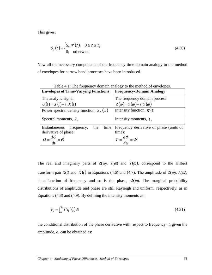
Chapter 4: Modeling of Phase Differences: Method of Envelopes 61
This gives:
( ) ( ) ≤≤
=otherwise;0
0;20 d
Z
TSS
ττητ (4.30)
Now all the necessary components of the frequency-time domain analogy to the method
of envelopes for narrow band processes have been introduced.
Table 4.1: The frequency domain analogy to the method of envelopes.Envelopes of Time-Varying Functions Frequency-Domain Analogy
The analytic signal
( ) ( ) ( )tXitXtU ˆ⋅+=The frequency domain process
( ) ( ) ( )ωωω YiYZ ˆ⋅+=Power spectral density function, ( )ωXS Intensity function, η2(t)
Spectral moments, nλ Intensity moments, nγ
Instantaneous frequency, the timederivative of phase:
ΘΘΩ ==dt
d
Frequency derivative of phase (units oftime):
ΦωΦΤ ′==
d
d
The real and imaginary parts of Z(ω), Y(ω) and ( )ωY , correspond to the Hilbert
transform pair X(t) and ( )tX in Equations (4.6) and (4.7). The amplitude of Z(ω), A(ω),
is a function of frequency and so is the phase, Φ(ω). The marginal probability
distributions of amplitude and phase are still Rayleigh and uniform, respectively, as in
Equations (4.8) and (4.9). By defining the intensity moments as:
( )∫= dT nn dttt
0
2ηγ (4.31)
the conditional distribution of the phase derivative with respect to frequency, τ, given the
amplitude, a, can be obtained as:
Chapter 4: Modeling of Phase Differences: Method of Envelopes62
( ) ∞<<∞−
∆−−
∆= τ
στττ
στπτ ;
2
1exp
2
12
aaaf
YY
AT (4.32)
where the mean phase derivative
[ ]0
1EγγτΦ ==′a (4.33)
represents the location (i.e. the time of occurrence) of the centroid of the intensity
function, ( )t2η , and
( ) 112
01
0221
20 −=−=γγγγ
γγγ∆T (4.34)
is a measure of how widely the intensity function is spread around its centroid. The
parameter T∆ is, therefore, a statistical measure of the effective duration of the process.
Analogous to Equation (4.18), the conditional variance of the phase derivative is given
by:
[ ]2
Var
⋅=′Y
T
aa
σ∆τΦ (4.35)
where 2Yσ is the variance of Y(ω).
In the following section the application of the method of envelopes and its
frequency domain analogy to the modeling of Fourier phase differences of earthquake
accelerograms is demonstrated.
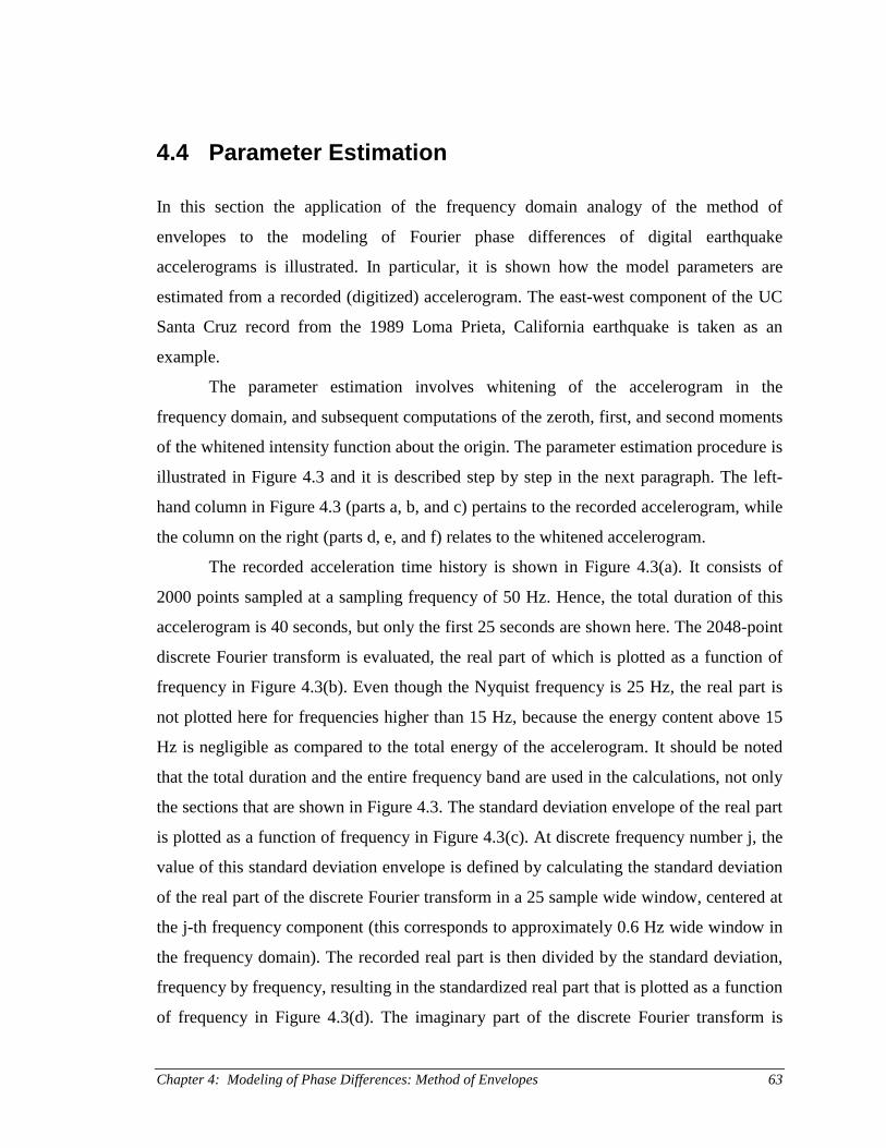
Chapter 4: Modeling of Phase Differences: Method of Envelopes 63
4.4 Parameter Estimation
In this section the application of the frequency domain analogy of the method of
envelopes to the modeling of Fourier phase differences of digital earthquake
accelerograms is illustrated. In particular, it is shown how the model parameters are
estimated from a recorded (digitized) accelerogram. The east-west component of the UC
Santa Cruz record from the 1989 Loma Prieta, California earthquake is taken as an
example.
The parameter estimation involves whitening of the accelerogram in the
frequency domain, and subsequent computations of the zeroth, first, and second moments
of the whitened intensity function about the origin. The parameter estimation procedure is
illustrated in Figure 4.3 and it is described step by step in the next paragraph. The left-
hand column in Figure 4.3 (parts a, b, and c) pertains to the recorded accelerogram, while
the column on the right (parts d, e, and f) relates to the whitened accelerogram.
The recorded acceleration time history is shown in Figure 4.3(a). It consists of
2000 points sampled at a sampling frequency of 50 Hz. Hence, the total duration of this
accelerogram is 40 seconds, but only the first 25 seconds are shown here. The 2048-point
discrete Fourier transform is evaluated, the real part of which is plotted as a function of
frequency in Figure 4.3(b). Even though the Nyquist frequency is 25 Hz, the real part is
not plotted here for frequencies higher than 15 Hz, because the energy content above 15
Hz is negligible as compared to the total energy of the accelerogram. It should be noted
that the total duration and the entire frequency band are used in the calculations, not only
the sections that are shown in Figure 4.3. The standard deviation envelope of the real part
is plotted as a function of frequency in Figure 4.3(c). At discrete frequency number j, the
value of this standard deviation envelope is defined by calculating the standard deviation
of the real part of the discrete Fourier transform in a 25 sample wide window, centered at
the j-th frequency component (this corresponds to approximately 0.6 Hz wide window in
the frequency domain). The recorded real part is then divided by the standard deviation,
frequency by frequency, resulting in the standardized real part that is plotted as a function
of frequency in Figure 4.3(d). The imaginary part of the discrete Fourier transform is

Chapter 4: Modeling of Phase Differences: Method of Envelopes64
standardized in a similar way. The standardized real and imaginary parts are stationary,
zero mean, unit variance stochastic processes as a function of frequency.
The whitened, discrete Fourier transform now consists of the standardized real
and imaginary parts. The whitened accelerogram, which is plotted as a function of time in
Figure 4.3(e), is obtained by evaluating the inverse, discrete Fourier transform of the
whitened Fourier transform. Note that this time history remains nonstationary in time,
though with roughly constant frequency content. The whitened intensity function, which
is shown in Figure 4.3(f), is simply the square of the whitened accelerogram. Now, the
whitened intensity moments can be calculated according to:
( ) 2,1,0;1
2 =⋅= ∑=
nttN
kk
nkn ηγ (4.36)
where N is the order of the discrete Fourier transform (equal to 2048 in this study), and
( )kt2η is the value of the whitened intensity function for the k-th sampling point in the
time domain. In this particular example, the whitened intensity moments are found to be:
2210 sec13.3sec,316.0,0377.0 === γγγ
which implies a centroid and a duration parameter equal to:
43.01sec,4.821
20
0
1 =−⋅
===γγγ∆
γγτ T

Chapter 4: Modeling of Phase Differences: Method of Envelopes 65
Figure 4.3: The whitening of an accelerogram. (a) The recorded east-west component ofthe UC Santa Cruz record from the 1989 Loma Prieta earthquake; (b) the real part of thediscrete Fourier transform (DFT) of the recorded accelerogram; (c) the evolutionarystandard deviation envelope of the real part of the discrete Fourier transform; (d) thestandardized real part; (e) the whitened accelerogram; (f) the whitened intensity function.
The frequency domain analogy of the method of envelopes does not only require
the standardized real and the imaginary parts to be stationary with respect to frequency,
but they also have to be Gaussian and uncorrelated for any given frequency component.
The Gaussianity of the standardized real and imaginary parts is investigated in Figure 4.4.
A skewness coefficient of zero and a coefficient of kurtosis equal to three implies a
Gaussian distribution. As can be seen from Figure 4.4, these criteria are met for all
practical purposes.

Chapter 4: Modeling of Phase Differences: Method of Envelopes66
Figure 4.4: Histograms of the standardized real (top) and imaginary parts (bottom) for theeast-west component of the UC Santa Cruz record from the 1989 Loma Prietaearthquake.
The correlation between the standardized real and imaginary parts is examined in
Figure 4.5. The calculated correlation coefficient is exactly zero to the fourth decimal
place, and the scatterplot exhibits no apparent pattern. It is, therefore, concluded that all
the relevant requirements for the frequency domain analogy have been met.
In Figure 4.6, the phase differences from the east-west component of the UC
Santa Cruz record from the 1989 Loma Prieta earthquake are plotted as a function of the
whitened Fourier amplitude. Superimposed on the dots representing the observations in
Figure 4.6 are the predicted mean phase difference (solid line) and the mean plus and
minus one standard deviation (dashed lines). The predicted moments of the conditional
phase difference distribution are obtained from Equations (4.33) and (4.35), multiplied by
the sampling frequency, ∆ω. It should be noted that the observed phase differences are
unwrapped to the finite interval [-π, π], while the predicted mean and standard deviation
are based on the assumption that the phase differences can take any real value. Therefore,
the observed scatter might not agree well with the predicted standard deviation,
especially for small amplitudes. Of course, this distinction between bounded and

Chapter 4: Modeling of Phase Differences: Method of Envelopes 67
unbounded phase definitions becomes immaterial once the inverse discrete Fourier
transform is taken to recover the time history.
Figure 4.5: Scatterplot of the standardized imaginary versus the standardized real part forthe east-west component of the UC Santa Cruz record from the 1989 Loma Prietaearthquake.
Figure 4.6: Observed unwrapped phase differences (dots) as function of the whitenedFourier amplitude (the amplitude is inferred from the standardized real and imaginaryparts) for the east-west component of the UC Santa Cruz record from the 1989 LomaPrieta earthquake. Superimposed are the mean (solid line) and mean +/- one standarddeviation (dashed lines) inferred from Equations (4.33) and (4.35).

Chapter 4: Modeling of Phase Differences: Method of Envelopes68
Even though the results presented in Figures 4.3 through 4.6 are for a particular
earthquake record, it should be noted that the analyses were performed on the entire
California ground motion database and the results presented above are typical for the
entire database. According to this, knowledge of the three whitened intensity moments is
sufficient to simulate the Fourier phase differences of digital accelerograms. In the
following section, the results of these analyses are used to develop prediction formulas
for the parameters of the phase difference model.
4.5 Model Parameters
In Section 4.4 it was shown that three parameters are sufficient to describe the phase
difference distribution of the whitened accelerogram: the zeroth, first, and second
intensity moments. After whitening, the zeroth moment, which is equal to the area under
the intensity function, is the same for all records. This leaves only two parameters to
describe the shape of the whitened intensity function: the first and the second moments.
In Figure 4.7, the second whitened intensity moment, 2γ as defined in Equation (4.31), is
plotted as function of the first whitened intensity moment, 1γ , for the database of
California ground motion records described in Chapter 2. These two moments are
obviously not independent of each other. The figure suggests a parabolic relationship
between them.
A constant zeroth moment of the whitened intensity function and a parabolic
relationship between the first and the second moments implies a constant duration
parameter, T∆ . This is corroborated in Figure 4.8, where the whitened duration parameter
does not seem to depend significantly on the source to site distance. It should be noted
that a constant duration parameter, T∆ , does not imply a constant duration. It does imply,
however, that the effective duration of the whitened accelerogram is proportional to the
centroid of the whitened intensity function, τ .
Since the whitened duration parameter seems not to depend on the distance, the
one remaining parameter, the centroid of the whitened intensity function, should be

Chapter 4: Modeling of Phase Differences: Method of Envelopes 69
sufficient to describe the distance dependence of the phase difference distribution. In
Figure 4.9, the centroid is plotted as a function of distance for the California ground
motion database. The centroid increases with distance. This behavior is expected, as the
energy tends to arrive later and to be distributed over a longer time interval with
increasing distance, due to the dispersion and scatter in the seismic wave train.
It is of interest to examine what effect the whitening of the accelerogram has on
the parameters of the intensity function, i.e. the centroid and the unitless duration
parameter. In Figure 4.10, the whitened intensity centroid is plotted as function of the
recorded intensity centroid, along with the straight line y = x. There is a certain
correlation apparent between the whitened and the recorded centroids. Therefore, the
whitened centroid indicates where the centroid of the energy release of the recorded,
unwhitened accelerogram is, i.e. it has a clear, physical meaning.
The relationship between the duration parameters of the whitened and recorded
accelerograms is shown in Figure 4.11. In general, the whitening has the tendency to
increase the duration of the.
Figure 4.7: The second whitened intensity moment as function of the first whitenedintensity moment for the California ground motion database.
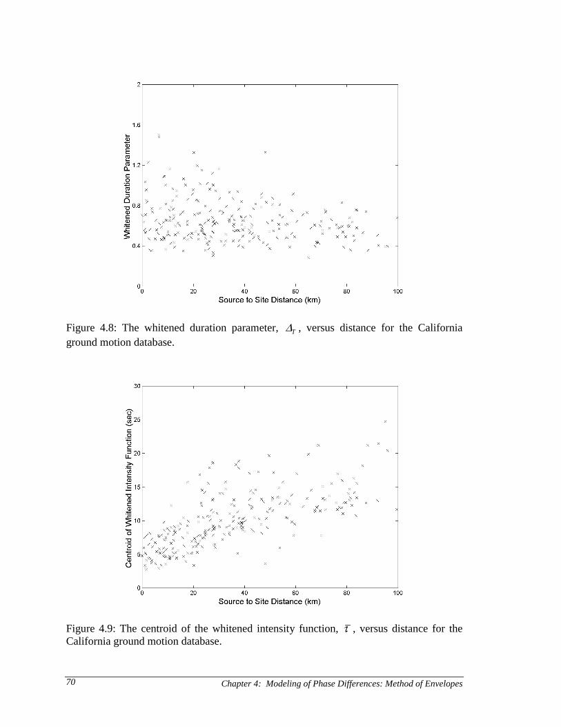
Chapter 4: Modeling of Phase Differences: Method of Envelopes70
Figure 4.8: The whitened duration parameter, T∆ , versus distance for the Californiaground motion database.
Figure 4.9: The centroid of the whitened intensity function, τ , versus distance for theCalifornia ground motion database.

Chapter 4: Modeling of Phase Differences: Method of Envelopes 71
Figure 4.10: The centroid of the whitened intensity function versus the centroid of therecorded intensity function for the California ground motion database.
Figure 4.11: The whitened duration parameter versus the recorded duration parameter forthe California ground motion database.

Chapter 4: Modeling of Phase Differences: Method of Envelopes72
It has been shown in this chapter that the probability distribution of Fourier phase
differences (Φ′ given their amplitude A) for digital earthquake accelerograms can be
described by a normal distribution, where the mean is constant and the standard deviation
is inversely proportional to the Fourier amplitude. Knowledge of two parameters,
T∆τ and , is sufficient to determine the mean and the conditional standard deviation of
the Fourier phase difference distribution; e.g. the centroid and the unitless width of the
whitened intensity function, or alternatively, the first and second whitened intensity
moments. In this section it was shown that the two parameters show strong statistical
dependence, indicating that only one parameter is sufficient to completely define the
phase difference distribution. In the following subsection, prediction formulas are
developed for the parameters of the normal distribution for Fourier phase differences.
The parameters chosen to describe the phase difference distribution are the first and
second temporal moments of the whitened intensity function, 1γ and 2γ , respectively.
The first moment is chosen as a primary parameter, i.e. dependent on magnitude and
distance, and the second moment is chosen as a secondary parameter, i.e. conditional on
the first moment.

Chapter 4: Modeling of Phase Differences: Method of Envelopes 73
4.5.1 The First Whitened Intensity Moment
The two-step regression procedure described in Section 2.2 is applied to the first
whitened intensity moment, 1γ . The functional form chosen for the regression analysis is
( )( )WM
c
Mc
Dccc 4321
1
exp ⋅⋅+=γ (4.37)
where D is the distance, and 1c , 2c , 3c , 4c , and ( )WM Mc are regression coefficients.
This functional form is chosen because it conforms to the observed pattern of the data
points. The coefficients ( )WM Mc are magnitude-dependent scaling factors. In the second
step of the regression procedure, a linear model is fitted to the magnitude scaling factors:
WM Mqqc ⋅+= 21 (4.38)
Here, 1q and 2q are regression coefficients, and WM is the moment magnitude of the
earthquake.
The results of the regression analysis using the entire California ground motion
data set are illustrated in Figure 4.12. In Figure 4.12(a), the magnitude-scaled first
whitened intensity moment is plotted as a function of the source to site distance. The
values of the regression parameters, obtained by non-linear least squares regression, are
given at the top of the figure. In Figure 4.12(b), the residuals from the regression in
Figure 4.12(a) are plotted as a function of distance. The standard deviation of the
residuals is determined to be 0.0485. The residuals do not appear to depend on distance.
A histogram of the standardized residuals is displayed in Figure 4.12(d). The coefficients
of skewness and kurtosis, which can be used when modeling the dispersion of the
residuals, if desired, are reported on the figure. The coefficient of skewness is 0.33,
implying a positive skewness, and the coefficient of kurtosis is 3.2, implying a
distribution that is slightly more peaked than the normal distribution. The results of the
second step of the regression procedure are shown in Figure 4.12(c), where the
magnitude scaling factor is regressed against moment magnitude. The scaling factor

Chapter 4: Modeling of Phase Differences: Method of Envelopes74
decreases with magnitude, implying that the first whitened intensity moment – hence τ
and the effective duration – increases with the magnitude of the earthquake. This is not
surprising, considering the longer source duration of the larger earthquakes.
Figure 4.12: Results of a two step regression analysis for the first whitened intensitymoment and all sites. (a) The distance dependence of the magnitude-scaled moment; (b)residuals from (a); (c) the magnitude dependent scaling factor; (d) histogram of thestandardized residuals from (a).
The two-step regression was repeated for Site Class A&B, Site Class C, and Site
Class D. The model parameters from these analyses are reported in Table 4.2, along with
the parameters that were obtained using recordings from the entire data set. The
parameter σ represents the standard deviation of the residuals from the regression.
The results of the regression analyses that are summarized in Table 4.2 are
displayed graphically in Figure 4.13. In Figure 4.13(a), the predicted magnitude-scaled
first moment is plotted as a function of distance for different site classes. The thick, solid

Chapter 4: Modeling of Phase Differences: Method of Envelopes 75
line in Figure 4.13(a) is the same as the solid line in Figure 4.12(a). The first moment is
considerably lower for Site Class A&B than the softer site classes, indicating that the
energy of accelerograms recorded at rock sites is concentrated closer to the beginning of
the record, than the energy of accelerograms that are recorded at soil sites. There does not
seem to be a significant difference between Site Class C, Site Class D, and All Sites, for
the magnitude-scaled first moment.
The magnitude dependency of the first whitened intensity moment is illustrated in
Figure 4.13(b) for different site classes. The thick, solid line in Figure 4.13(b) is the same
as the solid line in Figure 4.12(c). The magnitude scaling factor is most sensitive to the
magnitude for Site Class A&B, but it is practically identical for the other site classes.
Table 4.2: Regression results for 1γ (sec).Data Set
1c 2c 3c 4c 1q 2q σ
All Sites 0.295 -0.207 -0.0159 1.12 1.46 -0.143 0.0485
Site Class A&B 0.165 -0.139 -0.0303 1.12 3.19 -0.410 0.0186
Site Class C 0.274 -0.223 -0.0528 0.86 1.68 -0.177 0.0411
Site Class D 0.259 -0.141 -0.0002 2.65 1.45 -0.143 0.0311
Model:( )
W
c
Mqq
Dccc
⋅+⋅⋅+=
21
3211
4expγ
Figure 4.13: Results of a two-step regression analysis for the first whitened intensitymoment and different site classes. (a) The distance dependence of the magnitude-scaledmoment; (b) the magnitude dependent scaling factor.
Chapter 4: Modeling of Phase Differences: Method of Envelopes76
For prediction purposes, it is recommended to use the regression results from
Table 4.2 Site Class A&B, but to use the results pertaining to “All Sites” for all other site
classes. This recommendation is made despite the fact that the shape of the regression
curve for Site Class D in Figure 4.13(a) is different from the shape of all the other
regression curves in the figure. If the regression parameters pertaining to “All Sites” are
used, the standard prediction error – i.e. the standard deviation of the difference between
the observed and predicted magnitude-scaled 1γ – for Class D sites is 0.0402. While this
standard prediction error is one-third higher than the standard deviation of the residuals
obtained in the regression for Site Class D, it is still lower than the standard error
obtained in the regression for either “All Sites” or Site Class C. Therefore, it is
considered justifiable to use the regression results obtained from “All Sites” for Site
Class D.

Chapter 4: Modeling of Phase Differences: Method of Envelopes 77
4.5.2 The Second Whitened Intensity Moment
In the discussion of Figure 4.7 it was suggested that the second whitened intensity
moment would be a parabolic function of the first whitened intensity moment. The results
of such a regression analysis are shown in Figure 4.14. In Figure 4.14(a), the data points
are plotted as well as the best fit parabola, obtained by means of linear least squares
regression. The residuals from that regression are plotted as function of the first whitened
intensity moment in Figure 4.14(b). The histogram of the standardized residuals, which is
displayed in Figure 4.14(d), reveals a rather strong positive skewness and a very high
value of the coefficient of kurtosis. In Figure 4.14(c), the regression from 4.14(a) is
transformed into natural logarithm space.
Figure 4.14: Results of a polynomial regression of the second whitened intensity momentas function of the first whitened intensity moment. (a) The polynomial regression; (b) theresiduals from the regression in (a); (c) the regression in (a) transformed into naturallogarithm space; (d) histogram of the standardized residuals from (a).

Chapter 4: Modeling of Phase Differences: Method of Envelopes78
Figure 4.14(c) implies a linear relationship between the second and first whitened
intensity moments in natural logarithm space. The results of such linear regression
analysis are shown in Figure 4.15. In Figure 4.15(a), the best fit line, obtained by means
of linear least squares regression, is superimposed on the data points. In Figure 4.15(b),
the residuals from the linear regression are plotted as function of the independent
parameter; the natural logarithm of the first whitened intensity moment. A histogram of
the standardized residuals is displayed in Figure 4.15(d). The coefficients of skewness
and kurtosis, which are reported on that figure, are rather high, but considerably smaller
than those in Figure 4.14(d). The coefficient of skewness decreased from 1.24 to 0.83,
and the coefficient of kurtosis dropped from 5.84 to 4.00. In Figure 4.15(c), the
regression from 4.16(a) is transformed from natural logarithm space into linear space.
Figure 4.15: Results of a linear regression in natural logarithm space for the secondwhitened envelope moment as function of the first whitened envelope moment. (a) Thelinear regression in natural logarithm space; (b) the residuals from (a); (c) the regressionin (a) transformed into linear space; (d) histogram of the standardized residuals from (a).

Chapter 4: Modeling of Phase Differences: Method of Envelopes 79
Based on the more desirable behavior of the residuals of the regression analyses
presented in Figure 4.15 rather than the regression in Figure 4.14, the logarithmic
regression model (in Figure 4.15) is preferred over the quadratic polynomial fit to the
data (in Figure 4.14).
The linear regression was repeated for Site Class A&B, Site Class C, and Site
Class D. The model parameters from these analyses are reported in Table 4.3, along with
the parameters that were obtained using recordings from the entire data set. The
parameter σ represents the standard deviation of the residuals from the regression.
The results of the regression analyses that are summarized in Table 4.3 are
illustrated graphically in Figure 4.16. In Figure 4.16(a), the regression relationships are
presented in logarithmic space, and in Figure 4.16(b), the relationships are transformed
into linear space. There is negligible difference between the site classes. Therefore, it is
recommended to use the results in Table 4.3 pertaining to “All Sites” for all site classes.
Table 4.3: Regression results for 2γ (sec2).Data Set
1c 2c σ
All Sites 3.42 1.80 0.159
Site Class A&B 3.34 1.70 0.117
Site Class C 3.39 1.73 0.171
Site Class D 3.43 1.82 0.174
Model: ( ) ( )1212 lnln γγ ⋅+= cc
Figure 4.16: Results of a linear regression of the second whitened intensity momentversus the first whitened intensity moment for different site classes. (a) Logarithmicspace; (b) linear space.

Chapter 4: Modeling of Phase Differences: Method of Envelopes80
4.6 Model Validation
In Section 4.3 it was postulated that Fourier phase differences of digital earthquake
accelerograms could be modeled by a normal distribution, where the mean is independent
of the Fourier amplitude but the standard deviation is inversely proportional to the
amplitude. In this section, several tests are performed to estimate how well the assumed
model, i.e. the conditional normal distributions for Fourier phase differences, fit real
observations. Four different quality tests are performed: statistical goodness of fit tests
for the phase difference distributions, and three different tests where the characteristics of
simulated accelerograms are compared to the corresponding characteristics of recorded
accelerograms. These include comparisons of peak ground acceleration values, linear
response spectra, and the temporal distribution of the energy content. All four tests are
performed on the entire ground motion database that was used to develop the prediction
formulas for the model parameters.
4.6.1 Phase Difference Distributions
Figure 4.17 shows a comparison of the Fourier phase angle and phase difference
distributions between a recorded and a simulated accelerogram. The plots on the left hand
side are for the recorded east-west component at the UC Santa Cruz station in the 1989,
Loma Prieta earthquake. The plots on the right pertain to simulations, using conditional
normal distributions for the Fourier phase differences. The parameters of the normal
distribution are estimated according to the procedure described in Section 4.4, i.e., the
centroid sec 4.8=τ and the duration parameter 43.0=T∆ are found from a whitened
version of the recorded time history. The histograms of the phase angles, which are
displayed in Figures 4.17(a) and 4.17(b), reveal a relatively uniform pattern. The
histograms of phase differences, which are shown in Figures 4.17(c) and 4.17(d), are for
all practical purposes identical; the difference is negligible. In Figures 4.17(e) the
recorded phase differences are plotted as a function of the recorded Fourier amplitude,
and the simulated phase differences are plotted as a function of the recorded Fourier
amplitude in Figure 4.17(f). The gross characteristics of the scatterplot of the recorded
phase differences are reproduced in the scatterplot of the simulated phase differences.

Chapter 4: Modeling of Phase Differences: Method of Envelopes 81
Figure 4.17: Comparison of recorded and simulated Fourier phase angles and phasedifferences for the east-west component of the UC Santa Cruz record from the 1989,Loma Prieta earthquake. (a) Histogram of recorded phase angles; (b) histogram ofsimulated phase angles; (c) histogram of recorded phase differences; (d) histogram ofsimulated phase differences; (e) recorded phase differences vs. recorded Fourieramplitudes; (f) simulated phase differences vs. recorded Fourier amplitudes.

Chapter 4: Modeling of Phase Differences: Method of Envelopes82
Figure 4.17 provides a qualitative validation of the phase difference simulation
model for this particular record, but a general and quantitative validation method is
needed. Since the phase differences are simulated using a normal distribution, one might
think that a Kolmogorov-Smirnov test, similar to the tests that were performed for the
beta distributions in Subsection 3.4.1, might be useful. In the Kolmogorov-Smirnov
goodness of fit test, an assumed cumulative distribution function is compared to an
observed cumulative distribution function. Unfortunately, the Kolmogorov-Smirnov test
is not applicable to the phase difference distributions, because the probability distribution
of the recorded phase differences is not Gaussian as the assumed distribution is, due to
the effects of phase wrapping and truncation. The recorded phase angles are limited to a
2π-wide interval, for example the interval [-π, π]. Hence, the recorded phase differences
are limited to the interval [-2π, 2π], and after unwrapping, the interval [-π, π]. Therefore,
the recorded phase differences can never follow a normal distribution, not even a
truncated normal distribution. However, a two-sample Kolmogorov-Smirnov test can be
performed. In a two-sample Kolmogorov-Smirnov test, two empirical distributions are
compared and it is determined whether there is a significant difference between them.
The null-hypothesis is that the two observed distributions are different realizations of the
probability distribution of the same underlying random variable. If the difference between
the two observed distributions is not significant, the null-hypothesis is accepted. The true
distribution, i.e. the probability distribution of the underlying random variable, is not
necessarily known.
The simple choices for the two-sample Kolmogorov-Smirnov test are the
marginal distributions of recorded and simulated Fourier phase differences, or the
distributions of recorded and simulated Fourier phase angles. In Figure 4.18(a) the
cumulative probability distribution functions of the Fourier phase angles are plotted. The
solid line is the cumulative distribution for the accelerogram that was recorded at the UC
Santa Cruz station in the 1989, Loma Prieta earthquake (the east-west component). This
is the cumulative distribution that corresponds to the histogram in Figure 4.17(a). The
dashed line in Figure 4.18(a) represents the cumulative distribution of the simulated
phase angles; the cumulative distribution that corresponds to the histogram in Figure
4.17(b). The two phase angle distributions in Figure 4.18(a) are practically identical.

Chapter 4: Modeling of Phase Differences: Method of Envelopes 83
In Figure 4.18(b) the marginal cumulative phase difference distribution for the
recorded accelerogram (solid line, corresponding to the histogram in Figure 4.17(c)) is
plotted on top of the marginal distribution of the simulated phase differences (dashed
line, corresponding to the histogram in Figure 4.17(d)). The term “marginal phase
difference distribution” is used here because in this comparison, all the phase differences
are grouped together, independent of their Fourier amplitudes. The two marginal phase
difference distributions are nearly identical. It is hard to imagine a statistical goodness of
fit test that would reject the hypothesis that these two realizations come from the same
underlying distribution. However, the phase differences are simulated conditional on the
amplitudes. Therefore, any statistical goodness of fit test used to estimate the quality of
the simulation model should take this conditional characteristic into account. The
marginal distributions in Figure 4.18(b) do not.
Figure 4.18: Cumulative probability distribution functions for recorded (solid lines) andsimulated (dashed lines) phase angles (a) and phase differences (b). The east-westcomponent of the UC Santa Cruz record from the 1989, Loma Prieta earthquake.
In Figure 4.19(a), the recorded Fourier phase differences are plotted as a function
of the whitened Fourier amplitude – i.e. the amplitude after whitening of the
accelerogram in the frequency domain. This is the same plot as in Figure 4.6, except that
here the phase difference domain is [-1.4π, 0.6π], rather than [-π, π] as it is in Figure 4.6.
This domain-shift was performed so that the mean phase difference, represented by the
horizontal, solid line in the figure, would be in the center of the phase difference domain.
The dashed lines in the figure represent the mean phase difference plus/minus one

Chapter 4: Modeling of Phase Differences: Method of Envelopes84
standard deviation. Figure 4.19(b) is similar to Figure 4.19(a). The only difference is that
in Figure 4.19(b) the simulated phase differences, rather than the recorded phase
differences, are plotted as a function of the normalized Fourier amplitude. In Figures
4.19(c) and 4.19(d) the phase differences have been standardized, i.e. the mean phase
difference has been subtracted from each value and then divided by the standard
deviation corresponding to the particular normalized amplitude. Figure 4.19(c) shows
results for the recorded accelerogram, and Figure 4.19(d) for the simulated phase
differences. If the phase differences were not truncated, circular, or unwrapped, the dots
in Figures 4.19(c) and 4.19(d) would represent realizations of a standardized random
variable (zero mean, unit standard deviation), independent of the amplitude. This is
clearly not the case, especially for the lowest normalized amplitudes. As the normalized
amplitude approaches zero, the standard deviation, which is inversely proportional to the
normalized amplitude, approaches infinity. Hence, as the phase differences only take
finite values, the standardized phase difference approaches zero as the normalized
amplitude approaches zero. However, because the recorded and simulated phase
differences have been processed identically and their behavior conditional on the
normalized Fourier amplitude has been taken into account, the two-sample Kolmogorov-
Smirnov test can now be used to examine the validity of the phase difference modeling. It
does not matter that the underlying distribution is not known. The cumulative distribution
of the recorded standardized phase differences can be compared to the cumulative
distribution of the standardized simulated phase differences. If the difference between the
two cumulative distributions is insignificant, the phase difference simulation model is
accepted.

Chapter 4: Modeling of Phase Differences: Method of Envelopes 85
Figure 4.19: Standardization of phase differences for the east-west component of the UCSanta Cruz record from the 1989, Loma Prieta earthquake. (a) Recorded phasedifferences vs. whitened Fourier amplitudes; (b) simulated phase differences vs. whitenedFourier amplitudes; (c) standardized recorded phase differences vs. whitened Fourieramplitudes; (d) standardized simulated phase differences vs. whitened Fourieramplitudes.
The two-sample Kolmogorov-Smirnov goodness of fit test (sometimes also
referred to as the Smirnov test) is used to determine whether two observed cumulative
distribution functions are significantly different from each other. The statistic used to
estimate whether the two distributions are significantly different is the maximum of their
absolute difference:
( ) ( )xFxFS nnx
nn 2121 allmax −= (4.39)
Here, 21nnS is the Kolmogorov-Smirnov statistic, and ( )xFn1
and ( )xFn2 are the
cumulative distribution functions for samples of size 1n and 2n , respectively.

Chapter 4: Modeling of Phase Differences: Method of Envelopes86
The cumulative distribution functions for the two samples are given by:
( ) 2,1;,,2,1; === injn
jxF i
ijni
(4.40)
where jx is the j-th smallest observation. The assumption that the two samples are drawn
from the same population is rejected if the test statistic is larger than a certain critical
value, i.e. if
reject,2121⇒> crnnnn SS (4.41)
The critical value can be approximated by (Lindgren, 1976):
( )
+−=
21,
11
2
2ln21 nn
S crnn
α(4.42)
where α is the significance level of the test. The significance level is equal to the
probability of rejecting the null-hypothesis; the assumption that the two samples are
drawn from the same population, when the null-hypothesis true. The significance level is
usually chosen to be a small number, very often of the order of 0.01 to 0.10.
A discrete 2048 point Fourier transform yields 1024 unique observations of phase
difference (see Equation 3.7). The critical values for the two-sample Kolmogorov-
Smirnov statistic, calculated according to Equation (4.42), are given in Table 4.4, for
three different significance levels.
Table 4.4: Critical values of the two-sample Kolmogorov-Smirnov statistic for phasedifference distributions ( 102421 == nn ).
Significance Level Critical Value0.01 0.0719
0.05 0.0600
0.10 0.0541

Chapter 4: Modeling of Phase Differences: Method of Envelopes 87
Figure 4.20 shows examples of simulated (dashed lines) and recorded (solid lines)
probability distributions for the standardized phase difference. The maximum difference
between the two cumulative distribution functions is 0.0429. This number is smaller than
all the values in the right-hand column of Table 4.4, thus the basic assumption that the
recorded and simulated distributions are two realizations of the same underlying random
variable is not rejected at any of the three significance levels. The same holds true for the
entire California ground motion database.
Figure 4.20: Cumulative probability distribution functions for the standardized phasedifferences (in Figure 4.19) corresponding to a recorded (solid line) and a simulated(dashed line) accelerogram. The east-west component of the UC Santa Cruz record fromthe 1989, Loma Prieta earthquake.
As described above, the statistical goodness of fit of the conditional normal
distributions for phase differences is very good, as measured by the two-sample
Kolmogorov-Smirnov test. It is of more interest, however, whether the accelerograms
simulated using these probability distributions, adequately reproduce the relevant
characteristics of recorded accelerograms. In the following subsection, the attributes of
simulated accelerograms are compared to the corresponding attributes of recorded
accelerograms.

Chapter 4: Modeling of Phase Differences: Method of Envelopes88
4.6.2 Accelerograms
In this subsection, the characteristics of simulated accelerograms, using the conditional
phase difference distributions, are compared with the corresponding characteristics of
recorded accelerograms. Three different characteristics are compared: peak values, elastic
response spectra, and evolutionary behavior.
Peak Ground Acceleration
In Figure 4.21, an example of a recorded accelerogram is displayed, along with two
sample simulations. The gross characteristics of the recorded accelerogram are
reproduced in the simulated accelerograms. The average peak ground acceleration from
ten simulations is 0.46g and the standard deviation is 0.06g, while the recorded peak
ground acceleration is 0.41g.
Figure 4.21: Examples of simulated accelerograms using a conditional normaldistribution for the Fourier phase differences. The recorded east-west component of theUC Santa Cruz record from the 1989 Loma Prieta earthquake (top) and two examplesimulations (bottom two).

Chapter 4: Modeling of Phase Differences: Method of Envelopes 89
The results displayed in Figure 4.21 are typical for the entire ground motion data
base. In the vast majority of cases, the recorded PGA is within one standard deviation of
the mean of ten simulations, and in every case, the recorded PGA is within two standard
deviations of the mean.
Elastic Response Spectrum
The elastic response spectra are compared in Figure 4.22. The solid line represents the
elastic pseudo acceleration response spectrum of the recorded ground motion, assuming a
damping ratio equal to 5% of critical damping. The dashed lines in Figure 4.20 represent
the response spectra of ten simulated acceleration time histories. For all natural periods
depicted in the figure (from 0.1 seconds to 2 seconds), the response spectra of the
simulated time histories envelope the response spectrum of the recorded time history. The
results in Figure 4.20 are representative of the entire ground motion data set.
Figure 4.22: Elastic pseudo acceleration response spectra (5% damping). Dashed lines:ten simulations using a conditional normal distribution for the Fourier phase differences;solid line: the recorded response spectrum from the east-west component of the UC SantaCruz record from the 1989 Loma Prieta earthquake.

Chapter 4: Modeling of Phase Differences: Method of Envelopes90
Cumulative Normalized Arias Intensity
The evolutionary behavior of the simulated and recorded accelerograms is displayed in
Figure 4.23. It is quantified in terms of the cumulative normalized Arias intensity, which
is defined in Equation (3.17). The dashed lines in Figure 4.23 represent the cumulative
normalized Arias intensity obtained from ten simulations, while the solid line represents
the cumulative normalized Arias intensity of the recorded accelerogram. In general, the
simulated accelerograms seem to capture well the evolutionary characteristics of the
recorded accelerogram. The curves for the simulated accelerograms tend not to be as
jagged as the curves for the recorded accelerograms, indicating a smoother evolutionary
energy release.
Figure 4.23: Cumulative normalized Arias intensity. Dashed lines: ten simulations usinga conditional normal distribution for the Fourier phase differences; solid line: thecumulative normalized Arias intensity of the east-west component of the UC Santa Cruzrecord from the 1989 Loma Prieta earthquake.
This concludes the comparison of the characteristics of simulated accelerograms
to those of recorded ones. In general, the comparison is found to be good.
Chapter 4: Modeling of Phase Differences: Method of Envelopes 91
4.7 Summary of Conditional Normal Distributions
Applying a frequency domain analogy initially proposed by Nigam (1982) to the method
of envelopes for time-varying functions, it is shown that the Fourier phase differences of
digital accelerograms can be modeled by a normal distribution with a constant mean and
where the standard deviation is inversely proportional to the Fourier amplitude. The mean
and the conditional standard deviation can be computed from the zeroth, first, and second
intensity moments of the whitened accelerogram.
The California ground motion database is used to develop prediction formulas for
the model parameters. The results of the regression analyses are summarized below. The
parameter D is the shortest distance from the site to the surface projection of the
seismogenic rupture in kilometers, and WM is the moment magnitude of the earthquake.
The zeroth whitened intensity moment is a constant, given by:
0380.00 =γ
The zeroth intensity moment is a unitless parameter.
For all non-rock sites, or an unknown site classification, the first whitened
intensity moment is given by:
( )3.78.5 km, 100;
143.046.1
0159.0exp207.0295.0 12.1
1 ≤≤≤⋅−
⋅−⋅−= WW
MDM
Dγ
For Site Class A&B the first moment can be estimated according to:
( )3.78.5 km, 100;
410.019.3
0303.0exp139.0165.0 12.1
1 ≤≤≤⋅−
⋅−⋅−= WW
MDM
Dγ
The first whitened intensity moment has the unit of seconds.
The second whitened intensity moment can be derived from the first moment for
all sites according to:
( ) ( )12 ln80.142.3ln γγ ⋅+=
Chapter 4: Modeling of Phase Differences: Method of Envelopes92
The second whitened intensity moment has the unit of seconds squared.
An alternative to using the whitened intensity moments for the parameterization
of the Fourier phase difference distributions would be to use the centroid, τ , and the
unitless duration parameter, T∆ , of the whitened intensity function. However, the
intensity moments proved to be better suited for regression analyses.
The Fourier phase difference model is validated through extensive statistical
goodness of fit tests, as well as comparison of certain characteristics of the simulated and
recorded accelerograms. These characteristics are: (i) the peak ground acceleration, (ii)
the 5% damped elastic response spectrum, and (iii) the evolutionary behavior as
quantified by the cumulative normalized Arias intensity. In general, the comparison is
found to be good.

Chapter 5: Modeling of Fourier Amplitudes 93
CHAPTER 5MODELING OF FOURIER AMPLITUDES
The modeling of Fourier amplitude spectra of earthquake accelerograms in a closed
parametric form has received considerable attention in previous studies. The Fourier
amplitude spectrum dictates how the total energy of the accelerogram is distributed in the
frequency domain. The focus of this study is the nonstationary energy release in time,
through modeling of the Fourier phase angle differences. However, for the purpose of
completeness, two well-known Fourier amplitude models are reviewed in this chapter. In
addition, a simple alternative approach is proposed, where the Fourier amplitude
spectrum is represented by a scaled and truncated lognormal probability density function.
The statistics on the Fourier amplitude spectra that are used in this chapter are tabulated
in Appendix D. It should be emphasized that the Fourier phase difference models
presented in the previous chapters do not depend on a particular Fourier amplitude model
or any other specific spectral modeling.
5.1 Current Amplitude Models
Two popular Fourier amplitude models are reviewed in this section: the radiated source
spectrum and the filtered Kanai-Tajimi spectrum. The radiated source spectrum was first
introduced in seismology, but it is gaining popularity in engineering. The filtered Kanai-
Tajimi spectrum has been one of the most commonly used amplitude models in the
engineering community for the last decades. Given the necessary information, either of
these Fourier amplitude models can be used with the models of the Fourier phase
differences that were presented in the previous chapters.

Chapter 5: Modeling of Fourier Amplitudes94
5.1.1 Radiated Source Spectrum
The far-field Fourier amplitude spectrum of earthquake ground acceleration at a “hard
rock” site is often described in terms of an attenuated source spectrum (e.g. Boore, 1983):
( ) ( ) ( ) ( ) ( )ωωϕθωωωϕθω PRDRGMECRMA cc ⋅⋅⋅⋅= ,,,,,,,,,, 00 (5.1)
In Equation (5.1), C is a constant accounting for free-surface amplification and the
partition of the radiated energy into two horizontal components, A(·) denotes the
acceleration amplitude spectrum at the site, E(·) is the acceleration amplitude spectrum at
the source, G(·) is a function that accounts for the radiation pattern of the seismic waves
and geometric attenuation, D(·) is an anelastic attenuation function, and P(·) is a high-cut
filter. The term M0 denotes the seismic moment, ωc is the corner frequency of the source
spectrum, and the triple (θ, ϕ, R) describes the location of the site with respect to the
source in spherical coordinates. The distance from the source to the site is denoted by R
(R is used here as a generic distance parameter, because D is reserved for the shortest
distance from a site to the surface projection of a seismogenic rupture), and ω represents
circular frequency.
The constant C accounts for the free-surface amplification and the partition of the
radiated energy into two horizontal components. The free-surface amplification factor is
usually taken as equal to 2. If the energy in the ground motion is assumed to be equally
divided into two horizontal components, the source spectrum has to be divided by a
factor of 2 to get the amplitude spectrum for each component. Hence, in that case, the
factor C becomes 222 = (Atkinson and Boore, 1995).
The source spectrum most often used is based on the omega-squared model,
proposed by Brune (1970):
( ) ( )20
2
01
,,c
c
MME
ωωωωω+
⋅= (5.2)

Chapter 5: Modeling of Fourier Amplitudes 95
This source spectrum is called the omega-squared model because for frequencies larger
than the corner frequency, the Fourier amplitude spectrum for displacement goes down as
the frequency squared. The corner frequency can be related to the seismic moment
through the Brune stress drop parameter (Brune, 1970).
The G(·) function combines the effects of directivity and geometric attenuation.
For propagating S waves, G(·) is given by (Kasahara, 1981):
( ) ( )RV
RGS ⋅⋅⋅
=34
,,,
ρπϕθϕθ (5.3)
where Ψ(θ,ϕ) is the radiation pattern, ρ is the mass density of the medium, and VS is the
shear wave velocity.
The anelastic attenuation is due to frictional damping in the medium. It is usually
modeled using the following exponential form (Aki and Richards, 1980):
( ) ( )
⋅⋅
⋅−=SVQ
RRD
ωωω
2exp, (5.4)
where Q(ω) is the quality factor. The value of the quality factor depends on the medium
and it has to be evaluated empirically. Sometimes, it is assumed to be independent of
frequency.
The high-cut filter is intended to take into account the rapid decay of the
amplitude spectrum at high frequencies, which is usually observed in recordings of
earthquake ground acceleration. The filter is often characterized by the Kappa-filter
(Atkinson, 1996):
( ) ( )κωω 21exp −=P (5.5)
where the parameter κ has to be evaluated empirically. As used here, κ is the zero
distance intercept of the parameter κ(R) as originally defined by Anderson and Hough
(1984). In their definition of κ(R), they combined the effects of anelastic attenuation and
high frequency decay. Boore (1986) suggests an alternative high-cut filter:

Chapter 5: Modeling of Fourier Amplitudes96
( )( )8
max1
1
ωωω
+=P (5.6)
Here, ωmax is the cut-off frequency proposed by Hanks (1982), who attributes this cut-off
frequency to site effects, while Papageorgiou and Aki (1983) suggest that it is a source
effect.
The radiated source spectrum is very comprehensive, but it requires too detailed
knowledge of the source and the medium to be usable for all practical engineering
situations. Furthermore, different source spectra and radiation patterns have to be used for
each type of seismic waves. Therefore, a simpler Fourier amplitude model is sought for
this study.
Figure 5.1: Schematic representation of the Fourier amplitude spectrum for earthquakeground acceleration (Equation 5.1) in logarithmic space.

Chapter 5: Modeling of Fourier Amplitudes 97
5.1.2 Filtered Kanai-Tajimi Spectrum
An alternative model of the Fourier amplitude spectrum for earthquake ground
acceleration, and one that is considerably simpler than the model presented previously, is
based on the Kanai-Tajimi power spectral density (the relationship between power
spectral density and Fourier amplitude is described in subsection 1.1.2). The Kanai-
Tajimi power spectral density is obtained by filtering a stationary white noise process
through a Kanai-Tajimi filter (Kanai, 1957; Tajimi, 1960):
( ) ( )( )[ ] ( ) ∞<<∞−
+−
+= ω
ωωξωω
ωωξω ;
41
4102222
22
SSggg
ggKT (5.7)
where S0 is the power spectral density of the underlying white noise process (see Fig.
5.2(a)), and the parameters ωg and ξg can be interpreted as the characteristic frequency
and damping ratio of the ground, respectively. The Kanai-Tajimi filter amplifies the
frequencies around ωg, attenuates higher frequencies, but does not change the amplitude
of very low frequencies (Fig. 5.2(b)). The non-zero power spectral density for zero
frequency poses a problem, because the power spectral densities for velocity and
displacement are obtained by dividing ω2 and ω4, respectively, into the power spectral
density for acceleration. Therefore, the Kanai-Tajimi power spectral density is often
passed through a low-cut filter, resulting in a power spectral density function of the
following form (Clough and Penzien, 1975):
( ) ( )( )[ ] ( )
( ) ∞<<∞−+−
= ωωωωξωω
ωωω ;41 2222
4
KT
LCLCLC
LC SS (5.8)
The gain function for this low-cut filter is shown in Figure 5.2(c), and the resulting
filtered Kanai-Tajimi power spectral density is illustrated in Figure 5.2(d).
The filtered Kanai-Tajimi power spectral density requires the estimation of five
parameters: the intensity of the underlying white noise process, the characteristic
frequency and the damping ratio at the site, and the two low-cut filter parameters, which
can be site dependent. It is not straightforward to determine the site dependent

Chapter 5: Modeling of Fourier Amplitudes98
parameters. Therefore, a still simpler model for the Fourier amplitude spectrum is sought
in this study.
Figure 5.2: A low-cut filtered Kanai-Tajimi power spectral density as function ofnormalized frequency; ξg = 0.6, ξLC = 0.8 and ωLC = ωg/15. (a) The power spectraldensity of the noise process, (b) the Kanai-Tajimi power spectral density, (c) the low-cutfilter, (d) the filtered Kanai-Tajimi spectrum.
5.2 Lognormal Density Function as Amplitude Spectrum
Several functional forms were investigated in this study for the modeling of Fourier
amplitudes of earthquake ground acceleration. Among those were various probability
density functions, such as the beta, chi-squared, gamma, lognormal, Weibull and
Rayleigh distributions. It was found that, in general, a lognormal probability density
Chapter 5: Modeling of Fourier Amplitudes 99
function fits the observed spectra reasonably well. The lognormal probability density
function is given by:
( ) ( )[ ]0;
2
lnexp
2
12ln
2ln
ln
≥
−−= x
x
xxf
X
X
X
X σµ
πσ(5.9)
where Xlnµ is the logarithmic mean (the scale parameter) and Xlnσ is the logarithmic
standard deviation (the shape parameter). This functional form was chosen because it is
relatively simple, and yet it seems to be flexible enough to capture the gross
characteristics of most observed amplitude spectra. Sabetta and Pugliese (1996) also use
a lognormal density function to describe the Fourier amplitude spectrum.
In order to fit a lognormal density function to the amplitude spectrum, the
frequency axis is first normalized such that the value of 1.0 corresponds to the Nyquist
frequency. Then the amplitudes are scaled in such a way that the integral of the squared
amplitudes with respect to normalized frequency equals one. This scaling is performed to
facilitate the use of a probability density function. Finally, a lognormal probability
density function is fitted to the scaled spectrum using the method of moments.
As an example, the Fourier amplitude spectrum for the east-west component of
the UC Santa Cruz record from the 1989 Loma Prieta earthquake is shown in Figure
5.3(a) on a linear scale and in Figure 5.3(b) on a logarithmic scale. The recorded and
scaled spectrum is denoted by the solid gray line, while the fitted lognormal density
function is shown by the dashed black line. The lognormal density function achieves a
reasonable fit with the recorded spectrum.
Three parameters are needed to completely define the smoothed Fourier amplitude
spectrum. These parameters are: (1) the amplitude scaling factor, representing the total
energy of the accelerogram, and (2) the scale and (3) the shape parameter of the
lognormal probability density function, reflecting the central frequency and the spectral
bandwidth of the accelerogram, respectively. In the following section, the California
ground motion database is used to develop prediction formulas for the Fourier amplitude
parameters.

Chapter 5: Modeling of Fourier Amplitudes100
Figure 5.3: Scaled recorded Fourier amplitudes (solid gray line) versus normalizedfrequency and the fitted truncated lognormal probability density function (dashed blackline) for the east-west component of the UC Santa Cruz record from the 1989 LomaPrieta, California earthquake in (a) linear space, and (b) logarithmic space.
5.3 Model Parameters
As described in the previous section, the scaled Fourier amplitude spectrum of an
earthquake accelerogram can be modeled by a lognormal probability density function.
There are three parameters necessary to completely define the spectrum: The total energy
of the accelerogram, represented here by the sum of the squared Fourier amplitudes, and
the two parameters needed to determine the scale parameter and the shape parameter of
the lognormal probability density function. In this study, the parameters chosen to define
the lognormal probability density function are (1) the first moment of the squared Fourier
spectrum about the origin, and (2) the second central moment of the squared spectrum.
These two moments, representing the central normalized frequency and the bandwidth of
the Fourier amplitude spectrum, respectively, are computed from the digital Fourier
amplitude spectrum according to
∑
∑
=
=⋅
=2
0
2
22
0 2N
nn
n
N
n
F
A
AN
n
M (5.10)
Chapter 5: Modeling of Fourier Amplitudes 101
( )22
0
2
2
0
2
2
2FN
nn
N
nn
F MA
AN
n
V −⋅
=∑
∑
=
=(5.11)
Here, FM is the first spectral moment of the positive part of the two-sided amplitude
spectrum about the origin, and FV is the second, central spectral moment. nA represents
the Fourier amplitude of the n-th discrete frequency, and N is the order of the discrete
Fourier transform. The ratio ( )2Nn is equal to the normalized frequency of the n-th
frequency component. The spectral moments defined in Equations (5.10) and (5.11) are
related to the shape and scale parameters of the fitted lognormal probability density
function in the following manner:
+=
22ln 1ln
F
FX M
Vσ (5.12)
( ) 2ln2
1ln ln XFX M σµ −= (5.13)
The third Fourier amplitude parameter, the energy-like scaling factor, is the sum of the
squared Fourier amplitudes:
∑=
=2
0
2N
nnAE (5.14)
These three parameters, the central frequency parameter FM , the spectral bandwidth
parameter FV , and the energy parameter E , completely define the fitted, smooth
amplitude spectrum. In this section, the California earthquake ground motion data is used
to develop prediction formulas for the amplitude parameters.
The three Fourier amplitude parameters are not all independent of each other. In
Figure 5.4, the bandwidth parameter is plotted as function of the central frequency
parameter. In Figure 5.4(a), the parameters are plotted on a linear scale, while logarithmic
scales are used in Figure 5.4(b). There is a clear positive correlation between the two

Chapter 5: Modeling of Fourier Amplitudes102
parameters. The linear plot indicates that the dispersion in the relationship increases with
increasing central frequency. However, no such trend is apparent in the logarithmic plot.
Therefore, it is preferable to perform linear regression in the logarithmic space.
Figure 5.4: The relationship between the two spectral moments for the California groundmotion database; the spectral bandwidth parameter, FV , as function of the central
frequency parameter, FM , in (a) linear space, and (b) logarithmic space.
In Figure 5.5, the energy parameter, E , is plotted as function of the central
frequency parameter, FM . Note that the vertical scale is logarithmic, while the horizontal
scale is linear. There is no apparent correlation, the two parameters seem to be
independent of each other. Therefore, they are chosen as the independent parameters, and
the second central moment is regressed on the first moment.
Two step regression analyses are performed on (1) the energy parameter, and (2)
the central frequency parameter versus distance and magnitude. In addition, a regression
relationship is developed between the bandwidth parameter and the central frequency
parameter.

Chapter 5: Modeling of Fourier Amplitudes 103
Figure 5.5: The energy parameter, E , as function of the central frequency parameter,
FM , for the California ground motion database.
5.3.1 The Energy Parameter
The results of a two step regression of the parameter E versus distance and magnitude
using the entire California ground motion database are summarized in Figure 5.6. The
model used in the first step is given by:
( ) ( )( )WM
c
Mc
DcccE
4321 exp
ln⋅⋅+= (5.15)
where D is the distance, and 1c , 2c , 3c , 4c , and ( )WM Mc are regression coefficients.
This functional form is chosen because it conforms to the observed pattern of the data
points. The coefficients ( )WM Mc are magnitude-dependent scaling factors. In the second
step of the regression procedure, a linear model is fitted to the magnitude scaling factors:
WM Mqqc ⋅+= 21 (5.16)
Chapter 5: Modeling of Fourier Amplitudes104
Here, 1q and 2q are regression coefficients, and WM is the moment magnitude of the
earthquake.
The distance dependence of the magnitude-scaled natural logarithm of the energy
parameter is displayed in Figure 5.6(a). The equation of the regression curve is printed
across the top of the figure. Due to energy dissipation and geometric spreading of the
seismic waves, the energy content of the accelerograms decreases with distance. The rate
of the energy attenuation decreases with increasing distance. The residuals from this
regression are plotted in Figure 5.6(b) as function of distance. The residuals do not
exhibit a distance dependence. The standard deviation of the residuals is reported in the
lower right hand corner of Figure 5.6(b). A histogram of the standardized residuals is
displayed in Figure 5.6(d). The coefficient of skewness, which is reported in Figure
5.6(d), is practically zero and the coefficient of kurtosis is close to 3. This implies that the
residuals can be modeled by a normal distribution. The magnitude-dependent scaling
factor is displayed in Figure 5.6(c). As can be seen, it increases with magnitude,
confirming the general belief that the energy increases with earthquake magnitude.
The two-step regression was repeated for Site Class A&B, Site Class C, and Site
Class D. The model parameters from these analyses are reported in Table 5.1, along with
the parameters that were obtained using recordings from the entire data set. The
parameter σ represents the standard error of the regression; it is the standard deviation of
the residuals.
The results of the regression analyses that are summarized in Table 5.1 are
displayed graphically in Figure 5.7. In Figure 5.7(a), the predicted magnitude-scaled
natural logarithm of the energy parameter is plotted as a function of distance for different
site classes. The thick, solid line in Figure 5.7(a) is the same as the solid line in Figure
5.6(a). For short distances, the energy parameter does not seem to depend on the site
class, but the energy appears to attenuates faster with distance for the stiffer sites than the
softer sites.
The magnitude dependency of the energy parameter is illustrated in Figure 5.7(b)
for different site classes. The thick, solid line in Figure 5.7(b) is the same as the solid line
in Figure 5.6(c). The scaling factor is most sensitive to the magnitude for Site Class A&B
and it is least sensitive to the magnitude for Site Class D.

Chapter 5: Modeling of Fourier Amplitudes 105
Figure 5.6: Results of a two step regression analysis for the energy parameter, E, for allsites. (a) The distance dependence of the magnitude-scaled natural logarithm of theenergy parameter; (b) residuals from (a); (c) the magnitude dependent scaling factor; (d)histogram of the standardized residuals from (a).
Figure 5.7: Results of a two-step regression analysis for the energy parameter, E, fordifferent site classes. (a) The distance dependence of the magnitude-scaled naturallogarithm; (b) the magnitude dependent scaling factor.

Chapter 5: Modeling of Fourier Amplitudes106
Table 5.1: Regression results for E (g2).Data Set
1c 2c 3c 4c 1q 2q σ
All Sites -5.41 2.62 -0.073 0.74 -1.00 0.460 0.407
Site Class A&B -5.21 2.35 -0.028 1.24 -2.01 0.615 0.339
Site Class C -4.90 1.97 -0.057 1.03 -1.47 0.532 0.436
Site Class D -4.53 1.40 -0.019 1.36 -0.88 0.440 0.400
Model: ( ) ( )W
c
Mqq
DcccE
⋅+⋅⋅+=
21
3214exp
ln
5.3.2 The Central Frequency Parameter
The results of a two step regression analysis for the central frequency parameter, FM ,
using the entire California ground motion data base, are displayed in Figure 5.8. It can be
inferred from Figure 5.8(a) that the magnitude-scaled central frequency decreases very
slightly with distance. High frequency ground motion tends to attenuate faster with
distance than low frequency motion, causing the central frequency parameter to decrease
with distance. The residuals from the regression in Figure 5.8(a) are plotted as function of
distance in Figure 5.8(b). The residuals do not seem to depend on distance. A histogram
of the standardized residuals is displayed in Figure 5.8(d). The residuals exhibit a positive
skewness and the coefficient of kurtosis is 3.21. Therefore, the normal distribution might
not be proper to model the residuals. The magnitude dependency of the central frequency
parameter is indicated in Figure 5.8(c), where the magnitude dependent scaling factor is
regressed versus moment magnitude. The central frequency tends to decrease with
increasing magnitude. Larger earthquakes typically have larger rupture areas, implying
longer source duration and, hence, lower frequency content. Therefore, the central
frequency is expected to decrease with increasing magnitude.
The two-step regression was repeated for Site Class A&B, Site Class C, and Site
Class D. The model parameters from these analyses are reported in Table 5.2, along with
the parameters that were obtained using recordings from the entire data set. The
parameter σ represents the standard deviation of the residuals from the regression.

Chapter 5: Modeling of Fourier Amplitudes 107
The results of the regression analyses that are summarized in Table 5.2 are
displayed graphically in Figure 5.9. In Figure 5.9(a), the magnitude-scaled natural
logarithm of the central frequency parameter is plotted as a function of distance for
different site classes. The thick, solid line in figure 5.9(a) is the same as the solid line in
Figure 5.8(a). The central frequency parameter for Site Classes C and D are very similar,
and considerably lower than the central frequency parameter for Site Class A&B. In
addition, the central frequency parameter is consistently lower for Site Class D than for
Site Class C. This is to be expected, because the natural frequency of softer soils is lower
than the natural frequency of stiffer soils. It is also interesting to note that the central
frequency parameter for Site Class A&B decreases more rapidly with distance than the
central frequency parameter for either of the softer site classes, implying that the higher
frequencies attenuate faster with distance than the lower frequencies.
The magnitude dependency of the natural logarithm of the central frequency
parameter is illustrated in Figure 5.9(b) for different site classes. The thick, solid line in
Figure 5.9(b) is the same as the solid line in Figure 5.8(c). The magnitude scaling factor
for Site Class A&B is considerably more sensitive to the magnitude than the scaling
factor for the other site classes.
Table 5.2: Regression results for FM .Data Set
1c 2c 1q 2q σ
All Sites -1.03 -0.0010 1.09 -0.082 0.227
Site Class A&B -0.53 -0.0039 2.17 -0.248 0.297
Site Class C -1.07 0.0002 1.10 -0.083 0.253
Site Class D -1.12 -0.0019 0.80 -0.038 0.206
Model: ( )W
F Mqq
DccM
⋅+⋅+=
21
21ln

Chapter 5: Modeling of Fourier Amplitudes108
Figure 5.8: Results of a two step regression analysis for the central frequency parameterand all sites. (a) The distance dependence of the magnitude-scaled natural logarithm ofthe central frequency parameter; (b) residuals from (a); (c) the magnitude dependentscaling factor; (d) histogram of the standardized residuals from (a).
Figure 5.9: Results of a two-step regression analysis for the central frequency parameterfor different site classes. (a) The distance dependence of the magnitude-scaled naturallogarithm; (b) the magnitude dependent scaling factor.

Chapter 5: Modeling of Fourier Amplitudes 109
5.3.3 The Spectral Bandwidth Parameter
A linear regression is performed on the spectral bandwidth parameter versus the central
frequency parameter in natural logarithm space. The results of this regression, using the
California ground motion data base, are summarized in Figure 5.10. In Figure 5.10(a), the
regression line is superimposed on the observed data points. The results of the regression
are transformed into linear space in Figure 5.10(c). The residuals of the linear regression
in Figure 5.10(a) are plotted versus the independent parameter in Figure 5.10(b). No
particular trend is observed. A histogram of the standardized residuals is shown in Figure
5.10(d). The residuals exhibit slight negative skewness. The coefficient of kurtosis for the
residuals is 3.81, considerably larger than the value of 3 for a normally distributed
random variable.
The linear regression was repeated for Site Class A&B, Site Class C, and Site
Class D. The model parameters from these analyses are reported in Table 5.3, along with
the parameters that were obtained using recordings from the entire data set. The
parameter σ represents the standard deviation of the residuals from the regression.
The results of the regression analyses that are summarized in Table 5.3 are
displayed graphically in Figure 5.11. In Figure 5.11(a), the relationships are presented in
logarithmic space, and in Figure 5.11(b) they are in linear space. The thick, solid lines in
Figure 5.11 are the same as the solid lines in Figure 5.10. It is apparent from Figure 5.11,
that the relationship between the spectral bandwidth parameter, FV , and the central
frequency parameter, FM , is practically the same for Site Class A&B as it is for Site
Class C. These relationships are, in turn, very similar to the relationship between FV and
FM that were obtained using the entire ground motion data set. Therefore, it is
recommended to use the results from Table 5.3 pertaining to “All Sites” for all sites
except for the softest sites, Site Class D. The relationship between FV and FM for Site
Class D seems to be significantly different from all the other FV - FM relationships.

Chapter 5: Modeling of Fourier Amplitudes110
Figure 5.10: Results of a linear regression of the spectral bandwidth parameter versus thecentral frequency parameter for all sites. (a) The linear regression in natural logarithmspace; (b) the residuals from the regression in (a); (c) the regression in (a) transformedinto linear space; (d) histogram of the standardized residuals from (a).
Figure 5.11: Results of a linear regression of the spectral bandwidth parameter versus thecentral frequency parameter for different site classes. (a) Logarithmic space; (b) linearspace.

Chapter 5: Modeling of Fourier Amplitudes 111
Table 5.3: Regression results for FV .Data Set
1c 2c σ
All Sites -1.80 1.43 0.423
Site Class A&B -1.97 1.26 0.399
Site Class C -1.96 1.36 0.350
Site Class D -1.41 1.53 0.405
Model: ( ) ( )FF MccV lnln 21 ⋅+=
5.3.4 Examples of Predicted Fourier Amplitude Spectra
The effects of magnitude, distance, and site conditions on the Fourier amplitude spectra
are illustrated in Figure 5.12. The spectra in Figure 5.12 are evaluated using the
prediction formulas for the model parameters that are presented in the previous
subsections.
The two spectra in Figure 5.12(a) are for a relatively close-by (source to site
distance of 10 km) rock site (Site Class A&B), but two earthquakes of different moment
magnitudes; 6 and 7. The area under the curve corresponding to the larger earthquake is
larger than the area under the curve corresponding to the smaller event, indicating higher
intensity of the ground motion. The larger event has considerably greater low-frequency
content than the smaller event. The higher intensity and greater low-frequency content of
the larger earthquake as compared to the smaller event can be attributed to a bigger
rupture area.
The effects of distance on the predicted Fourier amplitude spectra can be inferred
from a comparison of the two dashed curves in Figure 5.12. In Figures 5.12(a) and
5.12(b), the dashed line represents the spectrum at a rock site due to a magnitude 7
earthquake. In Figure 5.12(a), the source to site distance is 10 km, while the distance is
60 km in Figure 5.12(b). In addition to a lesser energy at the larger distance as compared
to the shorter distance, the central frequency and the spectral bandwidth are also lower at
the larger distance than at the smaller distance. This difference in the shape of the spectra
is due to the faster attenuation with distance of the high-frequency ground motion than
the low-frequency ground motion.

Chapter 5: Modeling of Fourier Amplitudes112
The effects of site conditions on the Fourier amplitude spectra are shown in
Figure 5.12(b). The dashed line represents the spectrum at a site corresponding to Site
Class A&B (rock site), while the dash-dot line is the Fourier amplitude spectrum at a site
corresponding to Site Class D (sandy soils and stiff clays; Borcherdt, 1994). Both spectra
in Figure 5.12(b) are due to a magnitude 7 earthquake and for a source to site distance
equal to 60 km. The energy (and hence, the intensity) of the ground motion at the softer
site (Site Class D) is larger than the energy at the stiffer site. In addition, the central
frequency and the spectral bandwidth are lower at the softer site than at the stiffer site.
The differences between the spectra in Figure 5.12(b) are consistent with observations
made by other researchers (e.g., Seed et al., 1976; Borcherdt, 1994), that soft soils tend to
filter out the high-frequency motion and sometimes to magnify the motion at a certain
(relatively low) frequency.
Figure 5.12: Examples of predicted Fourier amplitude spectra. (a) Spectra for earthquakesof moment magnitude 7 (dashed line) and 6 (solid line), for Site Class A&B and 10 kmdistance; (b) spectra for Site Class D (dash-dot line) and Site Class A&B, for anearthquake of moment magnitude 7 and a source to site distance of 60 km.

Chapter 5: Modeling of Fourier Amplitudes 113
5.4 Summary of Amplitude Models
Two existing Fourier amplitude models, which can be used together with the Fourier
phase difference models presented in the previous chapters, were reviewed in this
chapter: the radiated source spectrum and the filtered Kanai-Tajimi power spectral
density.
The radiated source spectrum model is very comprehensive. However, there are
many parameters to be evaluated, and different source spectra and radiation patterns have
to be used for each type of seismic waves. Furthermore, some of these parameters may be
earthquake-specific. Therefore, the radiated source spectrum is not very well suited for
predicting the earthquake ground motion from future events.
In order to use the filtered Kanai-Tajimi power spectral density, it is necessary to
quantify five parameters. These include the intensity of the underlying white noise
process, the characteristic frequency and damping ratio of the ground, and the two low-
cut filter parameters. This model is significantly simpler to use than the radiated source
spectrum. In this study, however, it was decided to propose a still simpler model for the
Fourier amplitude spectrum; a model that easily lends itself to regression analyses for
ground motion prediction purposes.
The alternative Fourier amplitude model proposed in this chapter is based on the
lognormal probability density function. Only three parameters are needed to specify the
Fourier amplitude spectrum: (1) the amplitude scaling factor, representing the total
energy of the accelerogram, and (2) the scale and (3) the shape parameter of the
lognormal probability density function, reflecting the central frequency and the
bandwidth of the accelerogram, respectively.
The California ground motion database described in Chapter 2 is used to develop
prediction formulas for the Fourier amplitude parameters E, MF and VF. The results of the
regression analyses are summarized below. The parameter D is the shortest distance from
the site to the surface projection of the seismogenic rupture in kilometers, and WM is the
moment magnitude of the earthquake.
Chapter 5: Modeling of Fourier Amplitudes114
The energy parameter is the sum of the squared Fourier amplitudes of an
accelerogram that is digitized at a sampling frequency of 50 Hertz with a total duration of
40.98 seconds (2048 sample points). Its unit of measurement is g2, where g is the
acceleration of gravity at the surface of the Earth. The energy parameter is determined
from the source to site distance and the moment magnitude of the earthquake. For an
unknown site class, the energy parameter can be estimated according to:
( ) ( )3.78.5 km, 100;
00.1460.0
073.0exp62.241.5ln
74.0
≤≤≤−⋅
⋅−⋅+−= WW
MDM
DE
For Site Class A&B, the energy parameter can be calculated using:
( ) ( )3.78.5 km, 100;
01.2615.0
028.0exp35.221.5ln
24.1
≤≤≤−⋅
⋅−⋅+−= WW
MDM
DE
For Site Class C, the energy parameter is given by:
( ) ( )3.78.5 km, 100;
47.1532.0
057.0exp97.190.4ln
03.1
≤≤≤−⋅
⋅−⋅+−= WW
MDM
DE
For Site Class D, the energy parameter can be computed using:
( ) ( )3.78.5 km, 100;
88.0440.0
019.0exp40.153.4ln
36.1
≤≤≤−⋅
⋅−⋅+−= WW
MDM
DE
The central frequency parameter is determined from the source to site distance
and the earthquake magnitude. For an unknown site class, it can be estimated according
to:
( ) 3.78.5 km, 100;082.009.1
0010.003.1ln ≤≤≤
⋅−⋅−−= WW
F MDM
DM
For Site Class A&B, the central frequency parameter can be calculated using:
Chapter 5: Modeling of Fourier Amplitudes 115
( ) 3.78.5 km, 100;248.017.2
0039.053.0ln ≤≤≤
⋅−⋅−−= WW
F MDM
DM
For Site Class C, the central frequency parameter is given by:
( ) 3.78.5 km, 100;083.010.1
0002.007.1ln ≤≤≤
⋅−⋅+−= WW
F MDM
DM
For Site Class D, the central frequency parameter can be computed using:
( ) 3.78.5 km, 100;038.080.0
0019.012.1ln ≤≤≤
⋅−⋅−−= W
WF MD
M
DM
The spectral bandwidth parameter is derived from the central frequency
parameter. For Site Class D, the spectral bandwidth parameter can be estimated using:
( ) ( ) 41.1ln53.1ln −⋅= FF MV
For all other site classes than Site Class D (including unknown site classification), the
spectral bandwidth parameter is given by:
( ) ( ) 80.1ln43.1ln −⋅= FF MV


Chapter 6: Spatial Interpolation of Ground Motion 117
CHAPTER 6SPATIAL INTERPOLATION OF GROUND MOTION
Reliable information on earthquake ground motion at the location of a damaged structure
is necessary in order to investigate the causes of damage, and to correlate ground motion
to building damage. It is, however, very unlikely that a recording will be available for all
sites of interest. Hence, there is a need to obtain estimates of earthquake ground motion
through interpolation of earthquake accelerograms acquired from ground motion
recording stations.
The previous chapters dealt with the generation of earthquake ground motion at
individual sites. The time histories at different points were assumed to be independent of
each other, which is sufficient for the design or analysis of ordinary structures that are
small as compared to the wavelength of the propagating seismic waves. However, when
dealing with large structures, such as long-span bridges, pipelines and dams, the spatial
correlation of earthquake ground motion has to be taken into account. Whether the two
suspension towers of the Golden Gate bridge move in phase or out of phase, for instance,
has great effect on the response and the loading of the bridge.
In this chapter, a simple model for the spatial interpolation of earthquake ground
motion is developed. Data from the SMART-1 accelerometer array in Taiwan are used to
assess the accuracy of this model. The quantities being interpolated are the frequency
characteristics of the digital earthquake accelerograms, i.e. the Fourier amplitudes and
phase angles. This is motivated by the results of Chapters 3 and 4, which show the
importance of preserving phase information (more precisely, phase differences) to
simulate accelerograms at an individual site.

Chapter 6: Spatial Interpolation of Ground Motion118
6.1 Problem Statement and Basic Assumptions
Imagine the following scenario: An estimate is sought of the acceleration time history at
the site marked by the letter C in Figure 6.1. The distance between the epicenter and the
site is Cδ . No recordings were obtained at the site. However, there are recordings
available from adjacent recording stations; kP . The epicentral distance of station kP is
kδ . The distance between the site, C, and recording station kP is kd .
Figure 6.1: Schematic representation of the spatial interpolation problem. C marks thesite where the time history is sought; Pk are recording stations.
The Fourier amplitude of the n-th discrete frequency component at recording station kP
is denoted by ( )nkA ω and the Fourier phase angle of the same frequency component is
denoted by ( )nk ωΦ . When predicting the Fourier components ( )nkCA ω, and ( )nkC ωΦ , at
the site, C, from the corresponding components at recording station kP , the following two
basic assumptions are made.

Chapter 6: Spatial Interpolation of Ground Motion 119
• There is negligible energy attenuation or amplification, i.e. the Fourier amplitudes at
the site are equal to the amplitudes at the recording station:
( ) ( )nknkC AA ωω =, (6.1)
• Each frequency component propagates radially from the epicenter with a constant
apparent phase velocity, ( )nων . Hence, the Fourier phase angle can be predicted
according to the simple dispersion relationship:
( ) ( ) ( )( )n
nkCnknkC ων
ωδδωΦωΦ ⋅−−=, (6.2)
There are considerable difficulties in determining the apparent phase velocity a
priori since it depends on many factors, such as the type of wave (P-wave, S-wave,
Rayleigh, Love …), the properties of the medium, and the inclination of the wave ray
with respect to horizontal. However, several methods exist to estimate the apparent phase
velocity using available recordings; for example the Aligned Motion Method
(Harichandran and Vanmarcke, 1984), the Cross Correlation Method (Loh, 1985;
Oliviera, 1985), and the Frequency-Wave Number Method (Abrahamson and Bolt, 1987).
In the analyses on the data from the SMART-1 array performed in this study, estimates of
apparent wave velocity reported by Hao (1989) are used. These estimates were obtained
using the Frequency-Wave Number Method.
Equations (6.1) and (6.2) do not generally yield the same predictions at the site for
all recording stations. Therefore, the different predictions have to be combined in a “best
estimate” of some sort, using spatial interpolation. The remainder of this chapter
documents the search for that best estimate. Before going any further, however, the data
used to assess the accuracy of the interpolation model are introduced.
6.2 Data and Data Processing
Recordings of earthquake accelerograms from closely spaced recording stations are rare.
In this study, data from the SMART-1 array near Lotung in northeastern Taiwan are used
to validate the ground motion interpolation model. In this section, the geometry of the
array is described, as well as the data selection and data processing.

Chapter 6: Spatial Interpolation of Ground Motion120
6.2.1 The SMART-1 Array
The deployment of the SMART-1 accelerograph array is described by Bolt et al. (1982),
Abrahamson (1985), and Niazi (1990). The array consists of 39 tri-axial accelerographs
(see Figure 6.2); one central station, C-00, three concentric circles each containing 12
equally spaced stations, and two external stations, E-01 and E-02. The three circles are
named I (for Inner), M (for Middle), and O (for Outer). The stations in the circles are
numbered consequently from 01 to 12, starting from north counting clockwise. The
nominal radius of the inner circle is 200 meters, the radius of the middle circle is 1000
meters, and the radius of the outer circle is 2000 meters. The external stations are located
approximately 3 and 5 kilometers south of the central station. The geometry of the array
is illustrated in Figure 6.2 and a table with the coordinates and elevation of all the stations
is in Appendix E. The topography is very flat. The elevation of all but three stations is
between 2 and 10 meters. The lowest elevation is 2.4 m and the highest elevation is 18.1
meters.
Figure 6.2: The geometry of the SMART-1 accelerometer array in Lotung, Taiwan.

Chapter 6: Spatial Interpolation of Ground Motion 121
The SMART-1 array is located in an alluvial plain, where the ground water table
is at or near the ground surface. All stations except station E-02, which is located on a
rock outcrop, are on soil. The depth of the soil column ranges from 170 meters in the
southern end of the outer circle to 600 meters at the northern edge of the array. The
estimated shear wave velocities in the uppermost 31 meters are given in Table 6.1.
Table 6.1: Shear wave velocity profile at the SMART-1 array site (Hao, 1989).Depth (m) 0 – 5 5 – 8 8 – 13 13 – 31
VS (m/s) 120 140 190 220
According to the shear wave velocity profile in Table 6.1, a shear wave would travel
from a depth of 30 meters up to the surface in 0.167 seconds, which implies an average
shear wave velocity of 180 m/s. According to the NEHRP site classification, the site of
the SMART-1 array would be on the border between classes D and E (see Table 2.2), i.e.
on the border between Soil and Soft Soil. A more detailed description of the geology can
be found in Bolt et al. (1982) and Abrahamson (1985).
6.2.2 Data
Uncorrected digitized data from the SMART-1 array were obtained from the Earthquake
Strong Motion CD-ROM collection published by the National Oceanic and Atmospheric
Administration of the United States Department of Commerce (NOAA, 1996). The
records were processed the same way as the California data, as described in Chapter 2.
The ground motion records were selected based on the following four criteria:
(1) Earthquake surface wave magnitude of at least 5.5.
(2) Uncorrected horizontal peak ground acceleration of at least 0.05 g.
(3) Epicentral distance between 10 and 100 kilometers.
(4) Focal depth less than 20 km.
The first two criteria are based on the assumption that smaller earthquakes and weaker
ground motion do not pose a significant hazard to most structures. The third and fourth

Chapter 6: Spatial Interpolation of Ground Motion122
criteria are meant to reduce the effects of vertically propagating seismic waves. The
selection criteria enumerated above yielded records from four events, which are
summarized in Table 6.2.
Table 6.2: Events recorded by the SMART-1 array that are used in this study.Event
No.Date MS Lat
(ºN)Long(ºE)
Depth(km)
Dist†(km)
Type*
5 29-Jan-1981 5.7 24.43 121.90 11.1 30 R
33 12-Jun-1985 5.8 24.57 122.19 3.3 45 O-N
39 16-Jan-1986 5.8 24.76 121.96 10.2 22 N
45 14-Nov-1986 7.8 23.99 121.83 13.9 77 R
† The distance is calculated between the center of the array and the epicenter of the earthquake.* R represents reverse-slip, N is normal-slip, and O-N stands for oblique-normal-slip.
The information in Table 6.2 is taken from Niazi (1990), except for the surface wave
magnitudes, which are from Abrahamson et al. (1987).
6.2.3 Geometric Interpolation Schemes
Based on the geometry of the SMART-1 array, three basic geometric interpolation
schemes are defined: using station pairs, triangles, and circles to evaluate the quantity of
interest (i.e. the Fourier transform of an acceleration time history) at the site of concern.
The different geometric schemes are designed to examine the effect of the number of
known points on the quality of the interpolation, as well as the effect of the layout and the
spacing of stations on the quality. The quality of interpolation is measured in terms of the
standard error, i.e. the standard deviation of the difference between the interpolated and
the observed values.
The first geometric interpolation scheme involves using a pair of diametrically
opposite stations to estimate the quantity of interest at the central station, C-00. All three
stations are on a (nominally) straight line. The stations can be of equal distance from the
central station, e.g. I-04 and I-10, or of different distance, e.g. I-04 and M-10. Two basic
cases are examined: (i) the propagation-parallel case, where the line connecting the
stations is parallel to the direction of seismic wave propagation, and (ii) the propagation-

Chapter 6: Spatial Interpolation of Ground Motion 123
perpendicular case, where the line connecting the stations is perpendicular to the
direction of wave propagation.
Two different triangular interpolation schemes are defined from the geometry of
the SMART-1 array. The first one is to define a nominally equilateral triangle from three
stations in the same circle, and use the values at the corners to estimate the value of
interest at the central station. An example of an inner circle equilateral triangle is shown
in Figure 6.3. The distance from the known stations to the unknown one is 200 meters,
and the sides of the triangle are 340 meters long. Stations from the Middle and Outer
circles can also be used to form equilateral triangles, similar to the one shown in Figure
6.3.
Another triangulation possibility is to create an isosceles triangle, using the
central station and two stations from the middle circle, as shown in Figure 6.4. The
triangle in this figure can be used to estimate the value at station I-01 in the inner circle.
The sides of this triangle are 1000 meters and 890 meters long, and the distance between
the corner points and the interior point is 200 meters and 880 meters.
Figure 6.3: Equilateral inner circle triangle to predict values at the central station.

Chapter 6: Spatial Interpolation of Ground Motion124
Figure 6.4: Isosceles triangle to predict values at the inner circle stations.
The third basic geometric interpolation scheme is to use all the stations in a given
circle (inner, middle, or outer) to estimate the values at the central station.
In the following section, these geometric interpolation schemes are used to
spatially interpolate the Fourier transform of digital accelerograms.
6.3 Interpolation of Discrete Fourier Transforms
Interpolation involves evaluating the weighted average of observed quantities. The
discrete Fourier transform is a complex function, which can either be characterized by its
real and imaginary parts, or its amplitude and phase angle. Hence, two questions arise: (i)
how to assign the weights, and (ii) which quantities to interpolate.
It is common in spatial interpolation to define the weights to be inversely
proportional to the distance between points, raised to a certain power. In this study, the
weights are assigned inversely proportional to the squared distance between the station
where the quantity is known and the site where the quantity is to be estimated. By taking
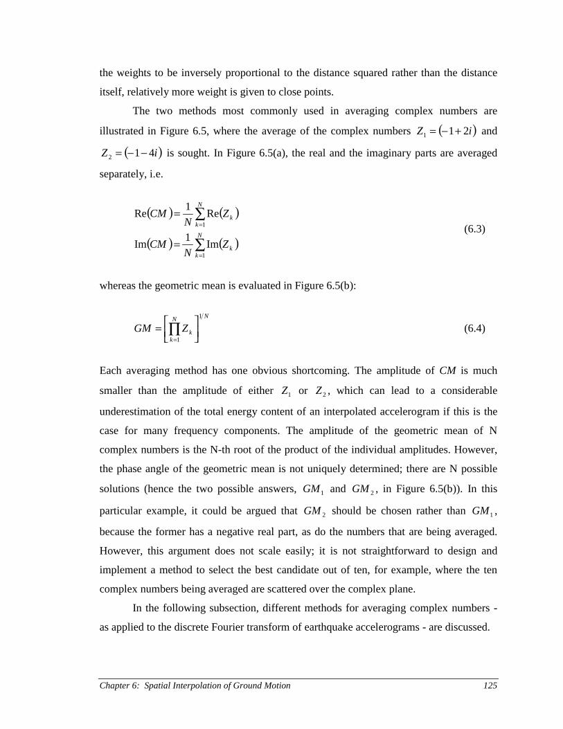
Chapter 6: Spatial Interpolation of Ground Motion 125
the weights to be inversely proportional to the distance squared rather than the distance
itself, relatively more weight is given to close points.
The two methods most commonly used in averaging complex numbers are
illustrated in Figure 6.5, where the average of the complex numbers ( )iZ 211 +−= and
( )iZ 412 −−= is sought. In Figure 6.5(a), the real and the imaginary parts are averaged
separately, i.e.
( ) ( )
( ) ( )∑
∑
=
=
=
=
N
kk
N
kk
ZN
CM
ZN
CM
1
1
Im1
Im
Re1
Re(6.3)
whereas the geometric mean is evaluated in Figure 6.5(b):
NN
kkZGM
1
1
= ∏
=(6.4)
Each averaging method has one obvious shortcoming. The amplitude of CM is much
smaller than the amplitude of either 1Z or 2Z , which can lead to a considerable
underestimation of the total energy content of an interpolated accelerogram if this is the
case for many frequency components. The amplitude of the geometric mean of N
complex numbers is the N-th root of the product of the individual amplitudes. However,
the phase angle of the geometric mean is not uniquely determined; there are N possible
solutions (hence the two possible answers, 1GM and 2GM , in Figure 6.5(b)). In this
particular example, it could be argued that 2GM should be chosen rather than 1GM ,
because the former has a negative real part, as do the numbers that are being averaged.
However, this argument does not scale easily; it is not straightforward to design and
implement a method to select the best candidate out of ten, for example, where the ten
complex numbers being averaged are scattered over the complex plane.
In the following subsection, different methods for averaging complex numbers -
as applied to the discrete Fourier transform of earthquake accelerograms - are discussed.

Chapter 6: Spatial Interpolation of Ground Motion126
Figure 6.5: Averaging the complex numbers Z1 and Z2. (a) The real and the imaginaryparts averaged separately; (b) the geometric mean.
6.3.1 Methods for Averaging Complex Numbers
As mentioned above, there are two basic methods for averaging complex numbers: (i)
averaging the real and the imaginary parts separately, and (ii) evaluating the geometric
mean. In this subsection, data from the SMART-1 array in Taiwan are used to estimate
the quality of these methods, as well as to propose a third and improved method for the
spatial interpolation of earthquake accelerograms in the frequency domain. The quality of
the different averaging methods is assessed by comparing the results of interpolations,
obtained using all the inner circle stations, to the accelerogram recorded at the central
station, C-00. All the numerical results presented in this subsection are for the north-
south component of Event 45 in Table 6.2.
In Figure 6.6, the recorded accelerogram is compared to an interpolated
accelerogram obtained by averaging the real and the imaginary parts separately. The
interpolated accelerogram looks like it has been passed through a low-pass filter, thus
removing the high-frequency energy. The lesser high-frequency content of the
interpolated time history as compared to the recorded one is obvious in Figure 6.7, where
the Fourier amplitude spectra of the two time histories are shown. The energy of the
interpolated accelerogram is lower, especially for the higher frequencies. Thus
confirming the doubts expressed in the discussion of Figure 6.5 regarding the
applicability of this method in averaging the discrete Fourier transforms of earthquake

Chapter 6: Spatial Interpolation of Ground Motion 127
accelerograms. However, as can be seen in Figure 6.8, averaging the real and imaginary
parts separately yields good estimates of the Fourier phase angles (and hence phase
differences). This agreement is particularly good at the relatively low frequencies (up to
10 Hz) where most of the accelerogram’s energy is located.
It is clear from Figures 6.6 and 6.7 that averaging the real and imaginary parts
separately can vastly underestimate the total energy in the earthquake accelerogram,
especially the high-frequency content (i.e. above 1 Hertz). However, as can be seen from
Figure 6.8, this averaging method gives very reasonable estimates of the Fourier phase
angle spectrum. Therefore, it is decided to use this averaging method to infer the Fourier
phase angles, while searching for another method to interpolate the Fourier amplitudes; a
method that better preserves the energy content.
The interpolated accelerogram in Figure 6.9 is obtained by evaluating the
geometric mean of the Fourier amplitudes of all the inner circle stations, while the
Fourier phase angles are inferred from the averages of the real and imaginary parts,
evaluated separately. The comparison with the recorded accelerogram is much better than
observed in Figure 6.6. However, by comparing the Fourier amplitude spectra in Figure
6.10, some energy deficiency is apparent, which becomes evident in Figure 6.11 where
the cumulative normalized Arias intensities are plotted as functions of time. It can be
seen in Figure 6.11 that the total energy of the interpolated accelerogram is only
approximately 70% of the total energy of the recorded accelerogram. Hence, evaluating
the geometric mean Fourier amplitude does not preserve the energy sufficiently well.

Chapter 6: Spatial Interpolation of Ground Motion128
Figure 6.6: The recorded acceleration time history at station C-00 (top) and theinterpolated time history (bottom) using all the recording stations of the inner circle,obtained by averaging the real and imaginary parts of the DFT’s separately.
Figure 6.7: The recorded Fourier amplitude spectrum at C-00 (solid line) compared to thespectrum of the interpolated time history (dashed line) using all the recording stations ofthe inner circle, obtained by averaging the real and the imaginary parts of the DFT’sseparately.
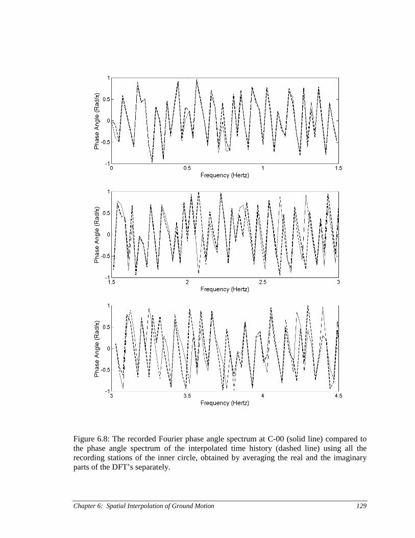
Chapter 6: Spatial Interpolation of Ground Motion 129
Figure 6.8: The recorded Fourier phase angle spectrum at C-00 (solid line) compared tothe phase angle spectrum of the interpolated time history (dashed line) using all therecording stations of the inner circle, obtained by averaging the real and the imaginaryparts of the DFT’s separately.

Chapter 6: Spatial Interpolation of Ground Motion130
Figure 6.9: The recorded acceleration time history at station C-00 (top) and theinterpolated time history (bottom) using all the recording stations of the inner circle,obtained by evaluating the geometric mean of the Fourier amplitudes, but inferring theFourier phase angles from averaging the real and imaginary parts separately.
Figure 6.10: The recorded Fourier amplitude spectrum at C-00 (solid line) compared tothe interpolated spectrum (dashed line) using all the recording stations of the inner circle,obtained by evaluating the geometric mean.

Chapter 6: Spatial Interpolation of Ground Motion 131
Figure 6.11: The cumulative normalized Arias intensity of the recording at C-00 (solidline) compared to the cumulative normalized Arias intensity of the interpolated timehistory (dashed line) in Figure 6.9. The cumulative intensities are normalized w.r.t. theArias intensity of the recorded accelerogram.
If the goal is to preserve the average energy of the recorded accelerograms in the
spatial interpolation, the squared Fourier amplitudes should be averaged. It is, therefore,
proposed here to average the squared Fourier amplitudes. The geometric average of the
Fourier amplitudes is never larger than the arithmetic average, which, in turn, is never
larger than the square root of the average of the squared amplitudes.
In Figure 6.12, the interpolated accelerogram is compared to the recorded
accelerogram. The interpolation is obtained by evaluating the average of the squared
Fourier amplitudes of all the recording stations in the inner circle, while the phase angles
are inferred from the averages of the real and imaginary parts, evaluated separately. The
comparison of the time histories seems good. The Fourier amplitude spectra and the
cumulative normalized Arias intensities of the two time histories are shown in Figures
6.13 and 6.14, respectively. There is still some energy deficiency apparent in the
interpolation. The Arias intensity of the interpolated time history is only approximately
85% of the Arias intensity of the recorded time history. However, this deficiency is due

Chapter 6: Spatial Interpolation of Ground Motion132
to the fact that the Arias intensity of the recordings made at the inner circle stations is on
the average 15% lower than the intensity of the recording made at the center.
Figure 6.12: The recorded acceleration time history at station C-00 (top) and theinterpolated time history (bottom) using all the recording stations of the inner circle,obtained by averaging the squared Fourier amplitudes, but inferring the Fourier phaseangles from averaging the real and imaginary parts separately.
Figure 6.13: The recorded Fourier amplitude spectrum at C-00 (solid line) compared tothe interpolated spectrum (dashed line) using all the recording stations of the inner circle,obtained by averaging the squared Fourier amplitudes.
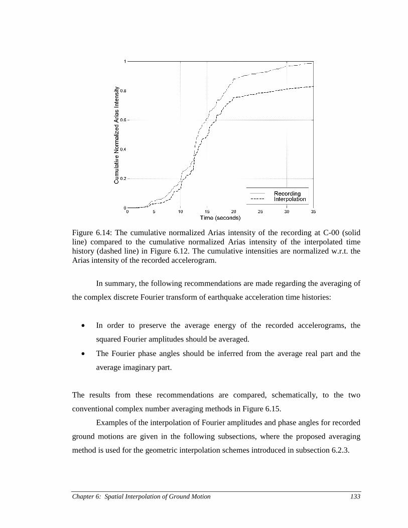
Chapter 6: Spatial Interpolation of Ground Motion 133
Figure 6.14: The cumulative normalized Arias intensity of the recording at C-00 (solidline) compared to the cumulative normalized Arias intensity of the interpolated timehistory (dashed line) in Figure 6.12. The cumulative intensities are normalized w.r.t. theArias intensity of the recorded accelerogram.
In summary, the following recommendations are made regarding the averaging of
the complex discrete Fourier transform of earthquake acceleration time histories:
• In order to preserve the average energy of the recorded accelerograms, the
squared Fourier amplitudes should be averaged.
• The Fourier phase angles should be inferred from the average real part and the
average imaginary part.
The results from these recommendations are compared, schematically, to the two
conventional complex number averaging methods in Figure 6.15.
Examples of the interpolation of Fourier amplitudes and phase angles for recorded
ground motions are given in the following subsections, where the proposed averaging
method is used for the geometric interpolation schemes introduced in subsection 6.2.3.

Chapter 6: Spatial Interpolation of Ground Motion134
Figure 6.15: Averaging the complex numbers 1Z and 2Z . The results of the proposedmethod, M, compared to results obtained by averaging the real and the imaginary partsseparately, CM, and by evaluating the geometric mean, 1GM or 2GM .
6.3.2 Interpolation of Fourier Amplitudes
For a given discrete frequency component, the interpolated Fourier amplitude at the site,
C, is evaluated as the square root of the weighted average of the squared amplitudes at
the recording stations. The relative weight for each station is inversely proportional to the
squared distance between the station and the site.
( ) ( ) ( )
2
22,
1
11
kk
knkk
kkk
nkCk
kk
nC
dw
Aww
Aww
A
=
⋅=⋅= ∑∑∑∑ωωω
(6.5)
In Equation (6.5), ( )nCA ω
is the interpolated Fourier amplitude corresponding to the n-th
discrete frequency, nω , at the site; ( )nkCA ω, is the Fourier amplitude at C as predicted

Chapter 6: Spatial Interpolation of Ground Motion 135
from recording station k, which is equal to the recorded Fourier amplitude at station k,
( )nkA ω , according to the assumption in Equation (6.1); kw is the weight assigned to
recording station k for prediction at the site; and kd is the distance between the site and
station k. In the simplest case of equally distant recording stations, the weights are all
equal and Equation (6.5) yields simply the square root of the average of the squared
amplitudes, as discussed previously.
In Figures 6.16 through 6.24, results from the amplitude interpolation model in
Equation (6.5) are compared to recordings made at the central station of the SMART-1
array. First, results from two-point interpolations are presented, followed by
interpolations using triangles and circles. The results presented here are all from Event
45, the largest event ever recorded by the SMART-1 array, but similar results were
obtained for all the other events listed in Table 6.2.
Two-Point Interpolation
In Figures 6.16 through 6.18, the recorded Fourier amplitude spectrum at station C-00 is
compared to the estimated spectrum at C-00, using two-point interpolation. The
interpolation in Figure 6.16 is obtained using a pair of inner circle stations, while the
interpolations in Figures 6.17 and 6.18 are obtained using a pair of middle circle stations
and outer circle stations, respectively. The interpolated Fourier amplitude spectrum
obtained using a pair of inner circle stations, where the station spacing is 200 meters,
compares well with the recorded amplitude spectrum; the standard error of the
interpolated amplitudes is 1.45·10-4 g. As may be expected, the frequency-by-frequency
comparison is not as good for the middle and outer circle interpolations as for the inner
circle interpolation. The standard error of the interpolated amplitudes is 2.44·10-4 g for the
middle circle interpolation, and the standard error is 2.84·10-4 g for the outer circle
interpolation. In general, there is not much difference in quality between middle and
outer circle interpolations, while the quality of the inner circle interpolations is
approximately twice as good as the quality of either the middle or the outer circle
interpolations. However, even though the interpolated spectra in Figures 6.17 and 6.18 do
not compare exactly to the recorded spectrum on a frequency by frequency basis, their
gross characteristics (i.e. the total energy, central frequency and bandwidth) are similar.

Chapter 6: Spatial Interpolation of Ground Motion136
Figure 6.16: The recorded Fourier amplitude spectrum at station C-00 (solid line)compared to the interpolated spectrum (dashed line) using the station pair (I-03,I-09).
Figure 6.17: The recorded Fourier amplitude spectrum at station C-00 (solid line)compared to the interpolated spectrum (dashed line) using the station pair (M-03,M-09).

Chapter 6: Spatial Interpolation of Ground Motion 137
Figure 6.18: The recorded Fourier amplitude spectrum at station C-00 (solid line)compared to the interpolated spectrum (dashed line) using the station pair (O-03,O-09).
Three-Point Interpolation
In Figures 6.19 through 6.21, the recorded Fourier amplitude spectrum at station C-00 is
compared to the estimated spectrum at C-00, using triangular interpolation. The
interpolation results shown in Figure 6.19 are for an equilateral, inner circle triangle, the
example in Figure 6.20 is for an equilateral middle circle triangle, and in Figure 6.21, the
interpolation results using an equilateral outer circle triangle are presented. The standard
error of the interpolated amplitudes is 1.39·10-4 g for the inner circle triangle, 2.66·10-4 g
for the middle circle triangle, and 2.67·10-4 g for the outer circle triangle. In general, the
quality of the triangular interpolation is slightly, but not significantly, better than the
quality of the two-point interpolations. Note in fact that in this particular case, the quality
of the three-point interpolation for the middle circle stations is a little worse than the
quality of the two-point interpolation. As in the two-point case, the gross characteristics
are reproduced by a coarse triangular interpolation (from middle or outer circle stations),
while the inner circle stations produce approximately twice the quality, on a frequency by
frequency basis.

Chapter 6: Spatial Interpolation of Ground Motion138
Figure 6.19: The recorded Fourier amplitude spectrum at station C-00 (solid line)compared to the interpolated spectrum (dashed line) using the triangle (I-03,I-07,I-11).
Figure 6.20: The recorded Fourier amplitude spectrum at station C-00 (solid line)compared to the interpolated spectrum (dashed line) using the triangle (M-03,M-07,M-11).

Chapter 6: Spatial Interpolation of Ground Motion 139
Figure 6.21: The recorded Fourier amplitude spectrum at station C-00 (solid line)compared to the interpolated spectrum (dashed line) using the triangle (O-03,O-07,O-11).
Interpolation using all the Stations in a given Circle
In Figures 6.22 through 6.24, the recorded Fourier amplitude spectrum at station C-00 is
compared to the interpolated spectrum at C-00, using recordings from all twelve stations
in a given circle. The interpolation results shown in Figure 6.22 are from the inner circle,
the example in Figure 6.23 is from the middle circle, and in Figure 6.24, the interpolation
results using all the stations of the outer circle are presented. The standard error of the
interpolated amplitudes is 1.27·10-4 g for the inner circle, 2.25·10-4 g for the middle circle,
and 2.44·10-4 g for the outer circle. In general, the quality of the twelve-point
interpolation is slightly better than the quality of the two-point and three-point
interpolations. As observed in the two- and three-point interpolations, the quality of the
inner circle interpolation is almost twice as good as the quality of the middle and outer
circle interpolations.
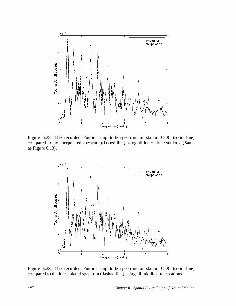
Chapter 6: Spatial Interpolation of Ground Motion140
Figure 6.22: The recorded Fourier amplitude spectrum at station C-00 (solid line)compared to the interpolated spectrum (dashed line) using all inner circle stations. (Sameas Figure 6.13).
Figure 6.23: The recorded Fourier amplitude spectrum at station C-00 (solid line)compared to the interpolated spectrum (dashed line) using all middle circle stations.

Chapter 6: Spatial Interpolation of Ground Motion 141
Figure 6.24: The recorded Fourier amplitude spectrum at station C-00 (solid line)compared to the interpolated spectrum (dashed line) using all outer circle stations.
Summary of Amplitude Interpolation
The Fourier amplitude interpolation model presented in Equation (6.5) yields quite
satisfactory results, at least with respect to the gross characteristics of the amplitude
spectra (the total energy, central frequency, and bandwidth). If the inter-station spacing is
less than 200 meters, the standard error of the interpolated Fourier amplitudes, frequency
by frequency, is on the average 40% to 50% less than if the spacing is larger than 1000
meters. Whether the spacing is 1 or 2 kilometers does not have much effect on the quality
of the interpolation, as measured by the standard error. Using twelve surrounding points
rather than two to interpolate the amplitude, and keeping the distance between the site
and the recording stations the same, lowers the standard error of the interpolation only by
10% to 15%, on the average. The interpolated Fourier amplitude spectrum becomes
smoother as more points are used in the interpolation and as the inter-station spacing
increases.

Chapter 6: Spatial Interpolation of Ground Motion142
6.3.3 Interpolation of Fourier Phase Angles
The interpolated Fourier phase angle of the n-th discrete frequency component at the site,
C, is inferred from the weighted averages of the real and imaginary parts of the predicted
discrete Fourier transforms:
( )( ) ( )( )[ ]( ) ( )( )[ ]
2
,,
,,
1
expRe
expImarctan
kk
knkCnkCk
knkCnkCk
nC
dw
jAw
jAw
=
⋅⋅⋅
⋅⋅⋅=
∑∑
ωΦω
ωΦωωΦ
(6.6)
In Equation (6.6) ( )nC ωΦ
is the interpolated Fourier phase angle corresponding to
discrete frequency nω at the site, C; ( )nkCA ω, is the Fourier amplitude at the site as
predicted by the recording at station number k; ( )nkC ωΦ , is the Fourier phase angle at the
site as predicted by the recording at station k; kw is the weight assigned to station number
k for prediction at the site; and kd is the distance between the site and station number k.
Recall from Section 6.1 that the Fourier amplitudes are assumed to stay the same, i.e.
( ) ( )nknkC AA ωω =, (6.1)
where ( )nkA ω is the Fourier amplitude of the n-th discrete frequency component of the
recording at station number k. Recall furthermore, that each frequency component is
assumed to propagate radially from the epicenter with a constant apparent phase velocity,
( )nων . Hence, the Fourier phase angle at the site can be predicted according to the simple
dispersion relationship:
( ) ( ) ( )( )n
nkCnknkC ων
ωδδωΦωΦ ⋅−−=, (6.2)
where ( )nk ωΦ is the Fourier phase angle of the n-th discrete frequency component of the
recording at station number k, Cδ is the epicentral distance of the site, and kδ is the
epicentral distance of station number k.

Chapter 6: Spatial Interpolation of Ground Motion 143
In Figures 6.25 through 6.35, results from the phase angle interpolation model
given in Equation (6.6) are compared to recordings for the geometric interpolation
schemes described in subsection 6.2.3. First, results from two-point interpolations are
presented, followed by results from triangular interpolations and interpolations using all
the recording stations of a given circle. The results presented here are all from Event 45,
the largest event ever recorded by the SMART-1 array, but similar results were obtained
for all the other events listed in Table 6.2.
Two-Point Interpolation
In Figures 6.25, 6.27 and 6.29, the recorded Fourier phase angle spectrum at station C-00
is compared to the estimated spectrum at C-00, using two-point interpolation. The
interpolation error (the observed phase angle minus the interpolated phase angle) is
plotted as function of frequency in Figures 6.26, and 6.28. The standard deviation of the
interpolation error for each 1.5 Hz wide frequency band is also reported in the figures.
The interpolation results presented in Figures 6.25 and 6.26 are for a propagation-
perpendicular pair of inner circle stations, while the results in Figures 6.27 and 6.28 are
from interpolation of a propagation-parallel inner circle pair. Due to lesser dispersion
effects, one would expect the interpolation from the propagation-perpendicular pair to
yield better results than the interpolation from the propagation-parallel pair. This
expectation can be confirmed, both by visual inspection and by comparing the standard
deviations of the interpolation errors reported in Figures 6.26 and 6.28. The comparison
between the recorded and interpolated phase angles is poorer for higher frequencies.
The interpolation results for a pair of propagation-perpendicular middle circle
stations are presented in Figure 6.29. The comparison between the recorded and the
interpolated phase angles is much poorer for the middle circle stations than the inner
circle stations. Since the comparison in Figure 6.29 is so poor, it is not thought necessary
to show the interpolation error as a function of frequency. The comparison is even worse
for a pair of propagation-parallel stations. Therefore, no example results of such
interpolation are shown.

Chapter 6: Spatial Interpolation of Ground Motion144
Figure 6.25: The recorded Fourier phase angle spectrum at station C-00 (solid line)compared to the interpolated phase spectrum (dashed line) using the propagation-perpendicular inner circle station pair (I-03,I-09).

Chapter 6: Spatial Interpolation of Ground Motion 145
Figure 6.26: The Fourier phase angle interpolation error at station C-00 for thepropagation-perpendicular inner circle station pair (I-03,I-09).

Chapter 6: Spatial Interpolation of Ground Motion146
Figure 6.27: The recorded Fourier phase angle spectrum at station C-00 (solid line)compared to the interpolated phase spectrum (dashed line) using the propagation-parallelinner circle station pair (I-06,I-12).

Chapter 6: Spatial Interpolation of Ground Motion 147
Figure 6.28: The Fourier phase angle interpolation error at station C-00 for thepropagation-parallel inner circle station pair (I-06,I-12).

Chapter 6: Spatial Interpolation of Ground Motion148
Figure 6.29: The recorded Fourier phase angle spectrum at station C-00 (solid line)compared to the interpolated phase spectrum (dashed line) using the propagation-perpendicular middle circle station pair (M-03,M-09).

Chapter 6: Spatial Interpolation of Ground Motion 149
Three-Point Interpolation
In Figures 6.30 and 6.32, the recorded Fourier phase angle spectrum at station C-00 is
compared to the estimated spectrum at C-00, using triangular interpolation. The
interpolation error (the difference between the observed and the interpolated phase angle)
obtained using an equilateral inner circle triangle is plotted as function of frequency in
Figure 6.31. The standard deviation of the interpolation error for each 1.5 Hz wide
frequency band is also reported in Figure 6.31.
The phase angle interpolation results presented in Figures 6.30 and 6.31 are for an
equilateral, inner circle triangle. The comparison between the recorded and interpolated
phase spectra is quite good, especially for frequencies lower than 3 Hz. It is interesting to
compare the results of this triangular interpolation to the results of the two-point
interpolation presented in Figures 6.25 through 6.28. Tthe quality of the triangular
interpolation is not significantly different from the quality of the interpolation using the
propagation-perpendicular pair (Figures 6.25 and 6.26), while the triangular interpolation
yields better results than the interpolation that uses the propagation-parallel station pair
(Figures 6.27 and 6.28).
The phase angle interpolation results presented in Figure 6.32 are from an
equilateral, middle circle triangle. This interpolation yields significantly worse results
than the interpolation from the inner circle triangle. The quality of the interpolation from
the middle circle triangle is similar to that from the wave-perpendicular, middle circle
pair, as shown in Figure 6.29.
The quality of the phase angle interpolation from an outer circle triangle is found
to be even poorer than the quality of interpolation from the middle circle triangle
described above. Therefore, the phase angle interpolation results from an outer circle
triangle are not shown here.

Chapter 6: Spatial Interpolation of Ground Motion150
Figure 6.30: The recorded Fourier phase angle spectrum at station C-00 (solid line)compared to the interpolated phase spectrum (dashed line) using the inner circle triangle(I-03,I-07,I-11).

Chapter 6: Spatial Interpolation of Ground Motion 151
Figure 6.31: The Fourier phase angle interpolation error at station C-00 for the innercircle triangle (I-03,I-07,I-11).

Chapter 6: Spatial Interpolation of Ground Motion152
Figure 6.32: The recorded Fourier phase angle spectrum at station C-00 (solid line)compared to the interpolated phase spectrum (dashed line) using the middle circletriangle (M-03,M-07,M-11).

Chapter 6: Spatial Interpolation of Ground Motion 153
Interpolation using all the Stations in a given Circle
In Figures 6.33 and 6.35, the recorded Fourier phase angle spectrum at station C-00 is
compared to the interpolated spectrum at C-00, using all the recording stations in a given
circle. The interpolation error (the observed phase angle minus the interpolated phase
angle) for the inner circle interpolation is plotted as function of frequency in Figure 6.34.
The standard deviation of the interpolation error for each 1.5 Hz wide frequency band is
also reported in Figure 6.34.
The phase angle interpolation results presented in Figures 6.33 and 6.34 are from
all the stations in the inner circle. The comparison between the recorded and interpolated
phase spectra is good for frequencies lower than 3 Hz. It is interesting to compare the
results of this interpolation to the results of the triangular interpolation, presented in
Figures 6.30 and 6.31, and the results of the propagation-perpendicular pair interpolation,
presented in Figures 6.25 and 6.26. It is seen that it does not make much difference
whether two propagation-perpendicular, three, or all twelve inner circle stations are used
to evaluate the Fourier phase angle at the central station through spatial interpolation.
The phase angle interpolation results presented in Figure 6.35 are from all the
stations in the middle circle. This interpolation yields significantly poorer results than the
interpolation from the inner circle. Furthermore, the quality of the phase interpolation
from all the middle circle stations is similar to that from the propagation-perpendicular
middle circle pair, as shown in Figure 6.29, and to the quality of the interpolation from
the middle circle triangle, as shown in Figure 6.32.
The quality of the phase angle interpolation using all the available recordings
from the outer circle is found to be even poorer than the quality of interpolation using the
middle circle stations, described above. Therefore, the phase angle interpolation results
from the outer circle are not shown here.

Chapter 6: Spatial Interpolation of Ground Motion154
Figure 6.33: The recorded Fourier phase angle spectrum at station C-00 (solid line)compared to the interpolated phase spectrum (dashed line) using all stations in the innercircle.

Chapter 6: Spatial Interpolation of Ground Motion 155
Figure 6.34: The Fourier phase angle interpolation error at station C-00 using all stationsin the inner circle.

Chapter 6: Spatial Interpolation of Ground Motion156
Figure 6.35: The recorded Fourier phase angle spectrum at station C-00 (solid line)compared to the interpolated phase spectrum (dashed line) using all stations in the middlecircle.

Chapter 6: Spatial Interpolation of Ground Motion 157
Summary of Phase Angle Interpolation
The Fourier phase angle interpolation model presented in Equation (6.6) yields
satisfactory results for inter-station spacing up to 200 meters and frequencies up to 3
Hertz. The model could possibly be extended up to a frequency of 4 Hertz and a spacing
of 500 meters, but not to frequencies or distances beyond these. When using only two
points to interpolate the phase angles, the line connecting the two points and the point for
which the phase angles are to be determined, should be perpendicular to the direction of
wave propagation. This increases the quality of the interpolation. The quality of the phase
angle interpolation is not significantly affected whether twelve or three points are used in
the interpolation. In either case, the quality of the interpolation is similar to the quality of
the interpolation from the propagation-perpendicular station pair.
6.4 Interpolated Time Histories
In the previous section, the quality of the spatial interpolation was evaluated in the
frequency domain. It is ultimately of considerable interest, of course, to study whether the
interpolated accelerograms, obtained by inverting the interpolated discrete Fourier
transform, closely resemble the recorded time histories in the time domain. In this
section, interpolated time histories are compared to the recorded time history at the
central station, C-00. The time histories themselves are compared, as well as their
nonstationary characteristics, as indicated by the cumulative normalized Arias intensity.
In view of the results of Chapters 3 and 4, it is anticipated that the cases in which the
Fourier phase differences (and hence the phase angles) are well predicted also show good
agreement in their nonstationary time domain characteristics.
In Figures 6.36 through 6.39 the results of two-point interpolations are compared
to the recorded ground motion at the central station, C-00. The two interpolated time
histories in Figure 6.36 are obtained using recordings from pairs of diagonally opposite
inner circle stations. The line connecting the pair I-03 and I-09 is perpendicular to the
direction of wave propagation, while the line connecting the pair I-06 and I-12 is parallel
to the direction of wave propagation. The interpolated time history obtained from the
propagation-perpendicular pair (the time history in the middle) resembles the recorded

Chapter 6: Spatial Interpolation of Ground Motion158
time history better than the interpolation obtained using the propagation-parallel pair (the
time history at the bottom). Note, for example, the build-up during the first 5 seconds,
and the strong shaking segment between the 10th and 20th seconds. The improvement in
results using the propagation-perpendicular interpolation rather than the propagation-
parallel interpolation is not surprising, because it was shown in the previous section that
the quality of the phase interpolation is better for a propagation-perpendicular pair than a
propagation-parallel pair.
The nonstationary characteristics of the two interpolated time histories in Figure
6.36 are compared to the nonstationary characteristics of the recorded time history in
Figure 6.37, where the cumulative normalized Arias intensities are shown as functions of
time. The cumulative intensity of each time history is normalized with respect to its own
Arias intensity. Hence, the curves are bounded between zero and one. The nonstationary
characteristics of the recorded time history and the two interpolated time histories are
very similar, as can be seen in Figure 6.37, where the three curves are nearly on top of
each other.
Figure 6.36: The recorded acceleration time history at station C-00 (top) and interpolatedtime histories (bottom two) using two diagonally opposite inner circle stations. The lineconnecting the pair (I-03,I-09) is perpendicular to the direction of wave propagation,while the line connecting I-06 and I-12 is parallel to the direction of wave propagation.

Chapter 6: Spatial Interpolation of Ground Motion 159
Figure 6.37: The cumulative normalized Arias intensities of the recording at station C-00(solid line) and the two interpolated time histories from Figure 6.36.
In Figure 6.38, the recorded time history at the central station is shown together
with three interpolated time histories. The interpolated time histories are all obtained
using recordings from a pair of propagation-perpendicular recording stations. The time
history at the bottom is from a pair of outer circle stations, the second from the bottom is
from a pair of middle circle stations, and the third from the bottom is from a pair of inner
circle stations. The inner circle interpolation, where the inter-station spacing is 200
meters, bears the closest resemblance to the recorded time history.
The cumulative normalized Arias intensities of the four time histories in Figure
6.38 are shown in Figure 6.39. The cumulative intensity of each time history is
normalized with respect to its own Arias intensity. The cumulative intensity curve for the
inner circle interpolation (the dashed line) is practically on top of the recorded cumulative
intensity curve (the solid line), while the cumulative intensity curves for the middle and
outer circle interpolations are somewhat different from the other two.
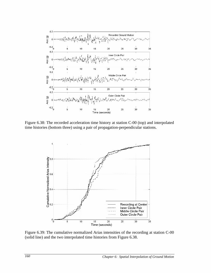
Chapter 6: Spatial Interpolation of Ground Motion160
Figure 6.38: The recorded acceleration time history at station C-00 (top) and interpolatedtime histories (bottom three) using a pair of propagation-perpendicular stations.
Figure 6.39: The cumulative normalized Arias intensities of the recording at station C-00(solid line) and the two interpolated time histories from Figure 6.38.

Chapter 6: Spatial Interpolation of Ground Motion 161
It has been shown that the characteristics of the two-point interpolations from the
middle and outer circle are not the same as the characteristics of the recorded time history
at the center, both in the time domain (in this section) and the frequency domain (in the
previous section). Nevertheless, it is interesting to note that these interpolations do yield
acceleration time histories whose characteristics are similar to those of recorded
earthquake accelerograms.
In Figure 6.40, the recorded acceleration time history at the central station, C-00,
is compared to three interpolated time histories, each obtained using recordings from
three inner circle stations that form an equilateral triangle. The three interpolations are
similar to each other and they are very similar to the recorded time history. The
nonstationary characteristics of all four time histories are shown in Figure 6.41, where the
cumulative normalized Arias intensities are plotted as functions of time. The cumulative
intensity of each time history is normalized with respect to its own Arias intensity. The
four cumulative intensity curves are practically on top of each other.
The quality of the three-point inner circle interpolations is comparable to, or only
slightly better than the quality of the interpolation using a pair of inner circle
propagation-perpendicular stations. Therefore, it could be argued that there is no need for
the third point in the interpolation. However, the quality of the three-point interpolations
is considerably better than the quality of the interpolation obtained from the propagation-
parallel pair. Since the quality of the three-point interpolations does not seem to depend
on the orientation of the triangle with respect to the direction of seismic wave
propagation, a three-point interpolation is, in general, preferred over a two-point
interpolation.

Chapter 6: Spatial Interpolation of Ground Motion162
Figure 6.40: The recorded acceleration time history at station C-00 (top) and interpolatedtime histories (bottom three) using inner circle triangles.
Figure 6.41: The cumulative normalized Arias intensities of the recording at station C-00(solid line) and the three interpolated time histories from Figure 6.40.

Chapter 6: Spatial Interpolation of Ground Motion 163
In Figure 6.42, the recorded acceleration time history at the central station, C-00,
is compared to three interpolated time histories, each obtained using recordings from
three stations that form an equilateral triangle. The time history at the bottom is from an
outer circle triangle, the time history second from the bottom is from a middle circle
triangle, and the time history second from the top is from an inner circle triangle. The
inner circle interpolation resembles best the recorded time history, while the outer circle
interpolation bears the worst resemblance to the recorded time history.
The cumulative normalized Arias intensities for all four time histories in Figure
6.42 are plotted as functions of time in Figure 6.43. The cumulative intensity of each time
history is normalized with respect to its own Arias intensity. Hence, the curves are
bounded between zero and one. The nonstationary characteristics of the three-point inner
circle interpolation (dashed line) and the recorded time history (solid line) are very
similar to each other, while the nonstationary characteristics of the three-point
interpolations for both the middle and outer circle stations are somewhat different from
the other two.

Chapter 6: Spatial Interpolation of Ground Motion164
Figure 6.42: The recorded acceleration time history at station C-00 (top) and interpolatedtime histories (bottom three) using equilateral triangles (stations 03, 07, and 11).
Figure 6.43: The cumulative normalized Arias intensities of the recording at station C-00(solid line) and the three interpolated time histories from Figure 6.42.
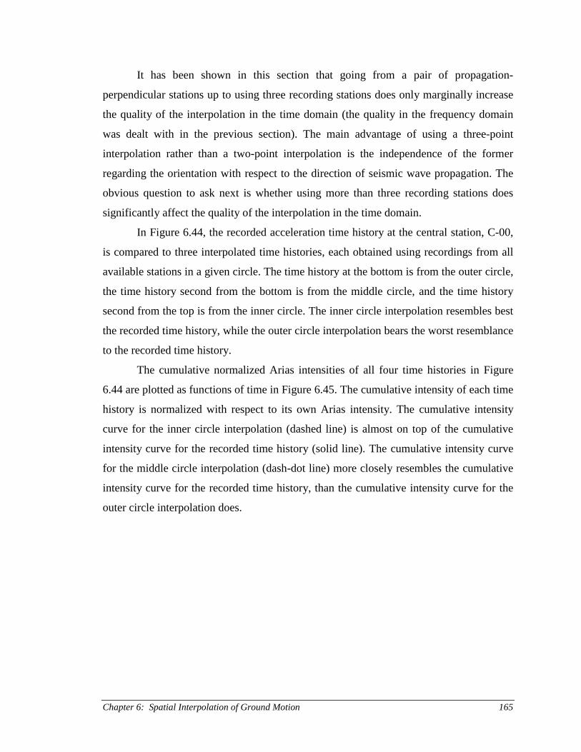
Chapter 6: Spatial Interpolation of Ground Motion 165
It has been shown in this section that going from a pair of propagation-
perpendicular stations up to using three recording stations does only marginally increase
the quality of the interpolation in the time domain (the quality in the frequency domain
was dealt with in the previous section). The main advantage of using a three-point
interpolation rather than a two-point interpolation is the independence of the former
regarding the orientation with respect to the direction of seismic wave propagation. The
obvious question to ask next is whether using more than three recording stations does
significantly affect the quality of the interpolation in the time domain.
In Figure 6.44, the recorded acceleration time history at the central station, C-00,
is compared to three interpolated time histories, each obtained using recordings from all
available stations in a given circle. The time history at the bottom is from the outer circle,
the time history second from the bottom is from the middle circle, and the time history
second from the top is from the inner circle. The inner circle interpolation resembles best
the recorded time history, while the outer circle interpolation bears the worst resemblance
to the recorded time history.
The cumulative normalized Arias intensities of all four time histories in Figure
6.44 are plotted as functions of time in Figure 6.45. The cumulative intensity of each time
history is normalized with respect to its own Arias intensity. The cumulative intensity
curve for the inner circle interpolation (dashed line) is almost on top of the cumulative
intensity curve for the recorded time history (solid line). The cumulative intensity curve
for the middle circle interpolation (dash-dot line) more closely resembles the cumulative
intensity curve for the recorded time history, than the cumulative intensity curve for the
outer circle interpolation does.

Chapter 6: Spatial Interpolation of Ground Motion166
Figure 6.44: The recorded acceleration time history at station C-00 (top) and interpolatedtime histories (bottom three) using all the recording stations in a given circle.
Figure 6.45: The cumulative normalized Arias intensities of the recording at station C-00(solid line) and the three interpolated time histories from Figure 6.44.

Chapter 6: Spatial Interpolation of Ground Motion 167
The question whether “more is better”, i.e. whether using twelve rather than three
recording stations in the spatial interpolation yields considerably better results has not yet
been answered. In Figure 6.46, the recorded acceleration time history at the central
station, C-00, is compared to three interpolated time histories, each obtained using
recordings from stations in the outer circle. The time history second from the top is
obtained using a pair of propagation-perpendicular stations (O-03 and O-09), the time
history second from the bottom is from an equilateral triangle (O-03, O-07, O-11), and
the time history at the bottom is obtained using all available recordings from the outer
circle.
The cumulative normalized Arias intensities of all four time histories in Figure
6.46 are plotted as functions of time in Figure 6.47. The cumulative intensity of each time
history is normalized with respect to its own Arias intensity. Hence, the curves are
bounded between zero and one.
The lesson learned from Figures 6.46 and 6.47 is that using more stations (i.e. the
entire circle, as opposed to either two or three stations) does not necessarily increase the
quality of the interpolation in the time domain. The time history at the bottom in Figure
6.46 bears the least resemblance to the recorded time history, and in Figure 6.47, the
nonstationary characteristics of the time history using the entire circle is most different
from the evolutionary characteristics of the recorded time history.
In subsections 6.3.2 and 6.3.3 it was shown that the interpolation quality in the
frequency domain increases only marginally when all the stations in a given circle are
used, as compared to using only two (propagation-perpendicular) or three stations. In the
time domain, the quality of the interpolation increases also marginally for the inner and
middle circle stations (radii of 200 meters and 1000 meters, respectively), but the quality
is slightly worse for the outer circle stations (nominal radius of 2000 meters). However,
the quality of the three-point interpolations is not orientation-dependent, but the quality
of the two-point interpolations is. It is therefore concluded that a three-point interpolation
scheme is effective for the spatial interpolation of earthquake ground motion.

Chapter 6: Spatial Interpolation of Ground Motion168
Figure 6.46: The recorded acceleration time history at station C-00 (top) and interpolatedtime histories (bottom three) using recordings from stations in the middle circle.
Figure 6.47: The cumulative normalized Arias intensities of the recording at station C-00(solid line) and the three interpolated time histories from Figure 6.46.
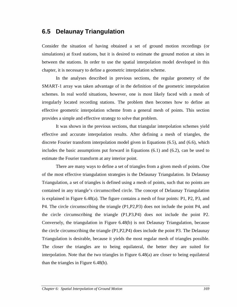
Chapter 6: Spatial Interpolation of Ground Motion 169
6.5 Delaunay Triangulation
Consider the situation of having obtained a set of ground motion recordings (or
simulations) at fixed stations, but it is desired to estimate the ground motion at sites in
between the stations. In order to use the spatial interpolation model developed in this
chapter, it is necessary to define a geometric interpolation scheme.
In the analyses described in previous sections, the regular geometry of the
SMART-1 array was taken advantage of in the definition of the geometric interpolation
schemes. In real world situations, however, one is most likely faced with a mesh of
irregularly located recording stations. The problem then becomes how to define an
effective geometric interpolation scheme from a general mesh of points. This section
provides a simple and effective strategy to solve that problem.
It was shown in the previous sections, that triangular interpolation schemes yield
effective and accurate interpolation results. After defining a mesh of triangles, the
discrete Fourier transform interpolation model given in Equations (6.5), and (6.6), which
includes the basic assumptions put forward in Equations (6.1) and (6.2), can be used to
estimate the Fourier transform at any interior point.
There are many ways to define a set of triangles from a given mesh of points. One
of the most effective triangulation strategies is the Delaunay Triangulation. In Delaunay
Triangulation, a set of triangles is defined using a mesh of points, such that no points are
contained in any triangle’s circumscribed circle. The concept of Delaunay Triangulation
is explained in Figure 6.48(a). The figure contains a mesh of four points: P1, P2, P3, and
P4. The circle circumscribing the triangle (P1,P2,P3) does not include the point P4, and
the circle circumscribing the triangle (P1,P3,P4) does not include the point P2.
Conversely, the triangulation in Figure 6.48(b) is not Delaunay Triangulation, because
the circle circumscribing the triangle (P1,P2,P4) does include the point P3. The Delaunay
Triangulation is desirable, because it yields the most regular mesh of triangles possible.
The closer the triangles are to being equilateral, the better they are suited for
interpolation. Note that the two triangles in Figure 6.48(a) are closer to being equilateral
than the triangles in Figure 6.48(b).
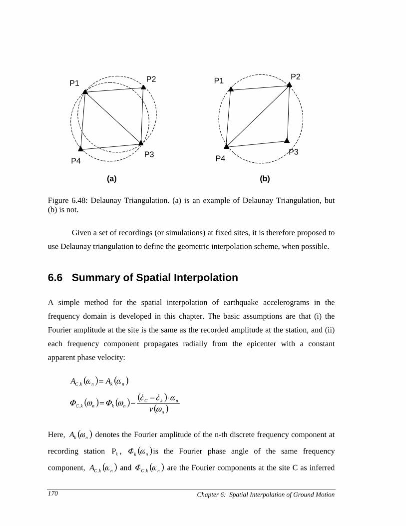
Chapter 6: Spatial Interpolation of Ground Motion170
P1 P2
P3P4
P1 P2
P3P4
(a) (b)
Figure 6.48: Delaunay Triangulation. (a) is an example of Delaunay Triangulation, but(b) is not.
Given a set of recordings (or simulations) at fixed sites, it is therefore proposed to
use Delaunay triangulation to define the geometric interpolation scheme, when possible.
6.6 Summary of Spatial Interpolation
A simple method for the spatial interpolation of earthquake accelerograms in the
frequency domain is developed in this chapter. The basic assumptions are that (i) the
Fourier amplitude at the site is the same as the recorded amplitude at the station, and (ii)
each frequency component propagates radially from the epicenter with a constant
apparent phase velocity:
( ) ( )nknkC AA ωω =,
( ) ( ) ( )( )n
nkCnknkC ων
ωδδωΦωΦ ⋅−−=,
Here, ( )nkA ω denotes the Fourier amplitude of the n-th discrete frequency component at
recording station kP , ( )nk ωΦ is the Fourier phase angle of the same frequency
component, ( )nkCA ω, and ( )nkC ωΦ , are the Fourier components at the site C as inferred

Chapter 6: Spatial Interpolation of Ground Motion 171
from station kP , Cδ is the epicentral distance of the site, kδ is the epicentral distance of
recording station kP , and ( )nων is the apparent propagation velocity of the n-th
frequency component.
The Fourier amplitudes are interpolated according to:
( ) ( )
2
2,
1
1
kk
knkCk
kk
nC
dw
Aww
A
=
⋅= ∑∑ωω
where kd is the distance between the site and the recording station kP . The phase angles
are interpolated using:
( )( ) ( )( )[ ]( ) ( )( )[ ]
2
,,
,,
1
expRe
expImarctan
kk
knkCnkCk
knkCnkCk
nC
dw
jAw
jAw
=
⋅⋅⋅
⋅⋅⋅=
∑∑
ωΦω
ωΦωωΦ
Data from the SMART-1 array in Taiwan are used to validate the Fourier
transform interpolation method, where interpolations are compared to recordings. The
Fourier amplitude interpolation model yields good results for inter-station spacing up to 2
kilometers. The quality of the phase angle interpolation is more dependent on spacing and
frequency than the amplitude interpolation. In general, the interpolated phase angles
compare well with the recorded ones for inter-station spacing up to 200 meters and
frequencies less than 3 Hz. The interpolated phase angles do not compare well with
recorded phase angles for frequencies over 5 Hz or inter-station spacing larger than 1
kilometer.
Even though the interpolated phase angles do not compare well with the recorded
ones for large inter-station spacings or high frequencies, the resulting time histories do
look realistic. Therefore, the spatial interpolation method developed in this chapter can be

Chapter 6: Spatial Interpolation of Ground Motion172
used to predict time histories for inter-station spacing larger than 1 kilometer, if it is not
desired to estimate the differential motion between the two sites.
It is shown that a triangular interpolation scheme is an effective way to yield
accurate results. A two-point interpolation can yield as good results as the triangular
interpolation, provided that the two interpolation points and the site at which the ground
motion is to be estimated are on a straight line that is perpendicular to the direction of the
seismic wave propagation. Using twelve points rather than three points does not produce
significantly better interpolation results.

Chapter 7: Case Study: The Northridge Earthquake 173
CHAPTER 7CASE STUDY: THE NORTHRIDGE EARTHQUAKE
In the preceding chapters, new models for the simulation and spatial interpolation of
earthquake ground motion were presented and validated. In this chapter, these models are
applied to the 1994 Northridge, California, earthquake. The intent is to demonstrate the
applicability of the models.
The Northridge earthquake occurred at 4:31 a.m. Pacific Standard Time on
January 17, 1994. The epicenter was at 118.54° West and 34.21° North (Hauksson and
Jones, 1995) in the San Fernando Valley, approximately 30 km west-northwest of
downtown Los Angeles. The moment magnitude of the earthquake was Mw = 6.7.
Analyses of seismograms imply an almost pure thrust motion on a plane striking north-
northwest and dipping down to the south-southwest. The earthquake originated at the
down-dip, southeastern corner of this plane (at a depth of 19 km) and ruptured upwards
and about 15 km to the northwest. Wald and Heaton (1994) found no evidence of slip
above 7 km depth.
Strong motion accelerograms from the Northridge earthquake were obtained from
more than two-hundred ground response stations throughout southern California. These
stations are operated by many different agencies, most of them by the California Division
of Mines and Geology, the U.S. Geological Survey, or the University of Southern
California. The study presented in this chapter only utilizes recordings from 45 stations
operated by the California Division of Mines and Geology. There are several reasons for
using data from only these 45 stations:
• By using sparse records from a single agency, the situation immediately following
a catastrophic event is better reproduced.
• Only records from stations within a certain distance interval are of interest; no
near-field records or weak-motion far-field records are included.
• Only uncorrected records from stations whose sensor properties (for signal
processing purposes) are readily available are used in this study.

Chapter 7: Case Study: The Northridge Earthquake174
A map showing the location of the recording stations with respect to the epicenter is
displayed in Figure 7.1. The stations that are used in this case study are tabulated in
Appendix F.
Figure 7.1: A map showing the location of the recording stations (dots) used in thischapter. The star marks the epicenter of the Northridge earthquake.
In the following section, ground motion intensity maps (showing peak ground
acceleration as well as spectral acceleration at selected natural periods) from simulated
time histories are compared to maps obtained from recordings in the Northridge
earthquake. In Section 7.2, the spatial interpolation method presented in Chapter 6 is used
to estimate the acceleration time history that a certain highway bridge, which collapsed in
the earthquake, is likely to have experienced.

Chapter 7: Case Study: The Northridge Earthquake 175
7.1 Ground Motion Intensity Maps
In this section, the results from the ground motion simulation model presented in
Chapters 4 and 5 are compared to recordings made in the Northridge earthquake. The
focus is on the east-west component of surface ground acceleration. The recordings at the
45 stations shown in Figure 7.1 are used to estimate the model parameters as function of
distance from the surface projection of the seismogenic rupture.
In Figures 7.2 through 7.5, the results of the simulations are compared to the
recordings, station by station. Ten simulations are performed at each location and the
mean and the mean plus or minus one standard deviation of various ground motion
intensity parameters are compared to those of the recorded ground motion. The ground
motion intensity parameters that are compared are the peak ground acceleration, and the
elastic, 5% damped pseudo spectral accelerations corresponding to natural periods of 0.3,
1.0 and 2.0 seconds. These natural periods are chosen because they are often taken as
representative of the fundamental periods for low-rise, mid-rise and high-rise steel frame
structures, respectively. The recorded ground motion intensity parameters and summary
statistics of the simulated ground motion intensity parameters are tabulated in Appendix
F.
The simulated peak ground accelerations are compared to the recorded peak
ground accelerations in Figure 7.2. In Figure 7.2(a) the relationship between the
simulated and recorded peak ground accelerations is plotted on a linear scale and in
Figure 7.2(b) the relationship is plotted on a logarithmic scale. The mean peak ground
accelerations from ten simulations are plotted, along with the mean +/- one standard
deviation, as functions of the recorded peak ground acceleration. The solid line represents
the line y = x. For 26 stations out of 45, the recorded peak ground acceleration is within
one standard deviation from the mean of the simulated peak ground accelerations. This
scatter is consistent with common statistical models. For example, 68% of all outcomes
will lie within one standard deviation of the mean for a Gaussian distribution.
The simulated spectral accelerations corresponding to natural periods of 0.3, 1.0
and 2.0 seconds are compared to the recorded spectral accelerations in Figures 7.3, 7.4
and 7.5, respectively. In general, the agreement of the spectral acceleration is better than
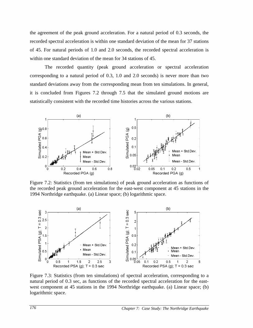
Chapter 7: Case Study: The Northridge Earthquake176
the agreement of the peak ground acceleration. For a natural period of 0.3 seconds, the
recorded spectral acceleration is within one standard deviation of the mean for 37 stations
of 45. For natural periods of 1.0 and 2.0 seconds, the recorded spectral acceleration is
within one standard deviation of the mean for 34 stations of 45.
The recorded quantity (peak ground acceleration or spectral acceleration
corresponding to a natural period of 0.3, 1.0 and 2.0 seconds) is never more than two
standard deviations away from the corresponding mean from ten simulations. In general,
it is concluded from Figures 7.2 through 7.5 that the simulated ground motions are
statistically consistent with the recorded time histories across the various stations.
Figure 7.2: Statistics (from ten simulations) of peak ground acceleration as functions ofthe recorded peak ground acceleration for the east-west component at 45 stations in the1994 Northridge earthquake. (a) Linear space; (b) logarithmic space.
Figure 7.3: Statistics (from ten simulations) of spectral acceleration, corresponding to anatural period of 0.3 sec, as functions of the recorded spectral acceleration for the east-west component at 45 stations in the 1994 Northridge earthquake. (a) Linear space; (b)logarithmic space.
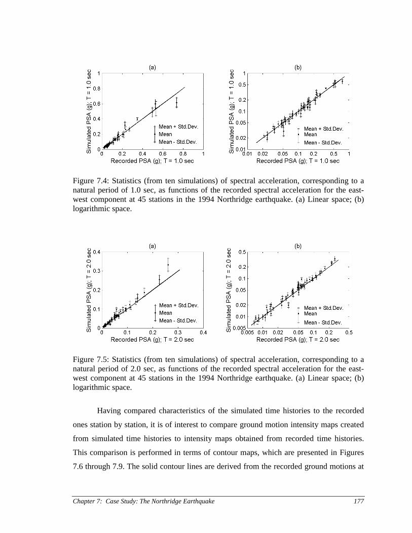
Chapter 7: Case Study: The Northridge Earthquake 177
Figure 7.4: Statistics (from ten simulations) of spectral acceleration, corresponding to anatural period of 1.0 sec, as functions of the recorded spectral acceleration for the east-west component at 45 stations in the 1994 Northridge earthquake. (a) Linear space; (b)logarithmic space.
Figure 7.5: Statistics (from ten simulations) of spectral acceleration, corresponding to anatural period of 2.0 sec, as functions of the recorded spectral acceleration for the east-west component at 45 stations in the 1994 Northridge earthquake. (a) Linear space; (b)logarithmic space.
Having compared characteristics of the simulated time histories to the recorded
ones station by station, it is of interest to compare ground motion intensity maps created
from simulated time histories to intensity maps obtained from recorded time histories.
This comparison is performed in terms of contour maps, which are presented in Figures
7.6 through 7.9. The solid contour lines are derived from the recorded ground motions at

Chapter 7: Case Study: The Northridge Earthquake178
the 45 recording stations shown in Figure 7.1. The dashed contour lines in Figures 7.6
through 7.9 are derived from simulated accelerograms. Ten simulations are performed at
each point of a rectangular grid and the quantity that is contoured is the average result
from the ten simulations. The grid is defined between 117.0 and 120.0 degrees west, and
between 33.5 and 35.5 degrees north. It has a constant spacing of 0.1 degrees, both in
latitude and longitude, which corresponds to approximately 9 km spacing in the east-west
direction and 11 km spacing in the north-south direction.
A contour map of the peak ground acceleration of the east-west component in the
Northridge earthquake is displayed in Figure 7.6. Contour maps for the spectral
acceleration corresponding to a natural period of 0.3, 1.0 and 2.0 seconds are shown in
Figures 7.7, 7.8 and 7.9, respectively. In general, the comparison between the simulated
and the recorded ground motion intensity maps is good. However, several observations
regarding their systematic differences can be made:
• The simulated contours for the 0.3 second spectral acceleration tend to be more
elongated towards the northwest than the recorded contours – especially those
representing spectral acceleration of 1.0 g and 1.5 g. This difference could be due
to a directivity effect, which is not captured by the simulation model.
• The simulated contours for the 2.0 second spectral acceleration tend to be outside
the corresponding recorded contours. This may imply a slight underestimation of
the attenuation in the simulation model for this long-period motion.
The relatively small differences that are observed between the recorded and simulated
contour maps are not necessarily due to shortcomings in the simulation model or in the
estimation of the model parameters. These differences could also be caused by the
different spatial distribution of the grid points as compared to the recording stations.
In this section, the applicability of the earthquake ground motion simulation model
for the generation of ground motion intensity maps over an entire region has been shown.
In the following section, the interpolation of ground motion time histories is
demonstrated.

Chapter 7: Case Study: The Northridge Earthquake 179
Figure 7.6: A contour map showing recorded (solid lines) and simulated (dashed lines)peak ground acceleration for the east-west component in the 1994 Northridge earthquake.
Figure 7.7: A contour map showing recorded (solid lines) and simulated (dashed lines)spectral acceleration, corresponding to a natural period of 0.3 sec, for the east-westcomponent in the 1994 Northridge earthquake.

Chapter 7: Case Study: The Northridge Earthquake180
Figure 7.8: A contour map showing recorded (solid lines) and simulated (dashed lines)spectral acceleration, corresponding to a natural period of 1.0 sec, for the east-westcomponent in the 1994 Northridge earthquake.
Figure 7.9: A contour map showing recorded (solid lines) and simulated (dashed lines)spectral acceleration, corresponding to a natural period of 2.0 sec, for the east-westcomponent in the 1994 Northridge earthquake.

Chapter 7: Case Study: The Northridge Earthquake 181
7.2 Interpolation of Time Histories
In order to correlate ground motion to building damage, it is necessary to have a
recording of a ground motion at the location of the damaged facility. This is very rarely
the case. Instead, one is faced with inferring the ground motion from near by, or in many
cases not so near by, recording stations. In Chapter 6, a method for the interpolation of
earthquake ground motion in the frequency domain was proposed. In this section, its
application is demonstrated by taking an example from the Northridge earthquake.
One of the highway bridges that collapsed in the Northridge earthquake was the
La Cienega and Venice undercrossing on the I-10 Santa Monica Freeway (bridge number
53-1609). It is located approximately 25 km southeast of the epicenter. The collapse of
this bridge was attributed to brittle shear failure of the concrete columns, due to
insufficient transverse reinforcement (Moehle et al., 1995). The bridge was designed and
constructed in the 1960’s.
To learn exactly what went wrong, however, it is not sufficient to only identify
the deficiencies in the design and construction of the bridge. To complete the picture, it is
necessary to obtain information on the ground motion at the site. No recordings were
obtained at the site. The three ground response stations closest to the site are Baldwin
Hills (BHA; epicentral distance of 28.1 km), the Hollywood Storage Building parking lot
(HSL; epicentral distance of 23.0 km) and the Century City Country Club (LCN;
epicentral distance of 20.2 km). These are shown on the map in Figure 7.10. The Baldwin
Hills station is located approximately 3.2 km south-southeast of the site, the Century City
station is about 5.2 km to the northwest, and the Hollywood Storage Building is roughly
6.6 km to the north-northeast of the bridge site. The site and the three recording stations
are all located in the Los Angeles Basin, with comparable local soil conditions.
In this section, the recorded time histories at Baldwin Hills, Century City, and the
Hollywood Storage Building are used to estimate the ground motion that the La Cienega
and Venice undercrossing on I-10 is likely to have experienced. First, a three-point
interpolation is used to estimate the ground motion at the site, using the triangular
interpolation scheme introduced and recommended in Chapter 6. Then, the effects of
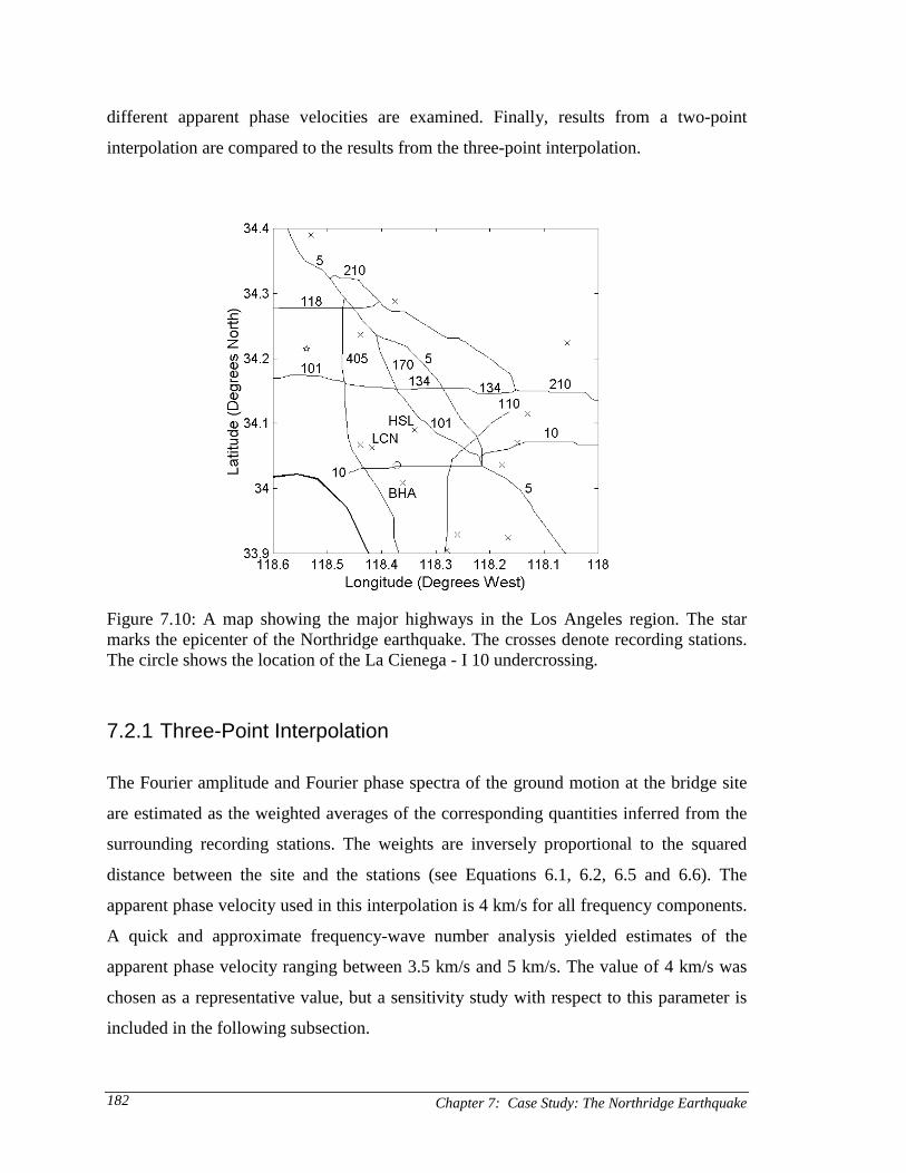
Chapter 7: Case Study: The Northridge Earthquake182
different apparent phase velocities are examined. Finally, results from a two-point
interpolation are compared to the results from the three-point interpolation.
Figure 7.10: A map showing the major highways in the Los Angeles region. The starmarks the epicenter of the Northridge earthquake. The crosses denote recording stations.The circle shows the location of the La Cienega - I 10 undercrossing.
7.2.1 Three-Point Interpolation
The Fourier amplitude and Fourier phase spectra of the ground motion at the bridge site
are estimated as the weighted averages of the corresponding quantities inferred from the
surrounding recording stations. The weights are inversely proportional to the squared
distance between the site and the stations (see Equations 6.1, 6.2, 6.5 and 6.6). The
apparent phase velocity used in this interpolation is 4 km/s for all frequency components.
A quick and approximate frequency-wave number analysis yielded estimates of the
apparent phase velocity ranging between 3.5 km/s and 5 km/s. The value of 4 km/s was
chosen as a representative value, but a sensitivity study with respect to this parameter is
included in the following subsection.

Chapter 7: Case Study: The Northridge Earthquake 183
The results of the interpolation of the east-west component of the acceleration are
shown in Figures 7.11 through 7.13, while the results for the north-south component are
displayed in Figures 7.14 through 7.16. Figures 7.11 and 7.14 show the recorded and
interpolated time histories. The time axis in all the graphs in this chapter starts at 2.8
seconds after 4:31 a.m. PST. All time histories are 41 seconds long (2048 points at 50 Hz
sampling frequency), but only the first 25 seconds are shown here. Figures 7.12 and 7.15
show the elastic, 5% damped pseudo acceleration response spectra, and Figures 7.13 and
7.16 show the cumulative, normalized Arias intensities. The Arias intensity of each time
history is normalized with respect to the Arias intensity (i.e., the total energy) of the
interpolated time history. Hence, the nonstationary characteristics as well as the total
energy of the recorded time histories can easily be compared to the corresponding
attributes of the interpolated time history on a single plot.
The recorded east-west components and the interpolated time history are shown in
Figure 7.11. The recorded peak ground accelerations are 0.26 g, 0.23 g and 0.24 g, at
stations LCN, HSL and BHA, respectively. The peak ground acceleration of the
interpolated time history is 0.24 g. The response spectrum of the interpolated time history
is similar to the response spectra of the recorded time histories, as shown in Figure 7.12.
The nonstationary characteristics and the total energy of the time histories are compared
in Figure 7.13. Everything is as expected. The total energy at the stations closer to the
epicenter than the site (LCN and HSL) is larger than the total energy of the interpolated
time history, and the total energy at the station that is farther away from the epicenter
(BHA), is smaller than the energy of the interpolated time history. Furthermore, the
cumulative intensity curves in Figure 7.13 never cross each other. The cumulative energy
at the site is always larger than the cumulative energy at BHA, while it is always smaller
than the cumulative energy at HSL. The cumulative energy at LCN, the recording station
that is closest to the epicenter, is always larger than the cumulative energy at any of the
other three locations.

Chapter 7: Case Study: The Northridge Earthquake184
Figure 7.11: The east-west component of the recorded acceleration time histories atstations LCN, HSL and BHA, and the interpolated time history.

Chapter 7: Case Study: The Northridge Earthquake 185
Figure 7.12: The elastic, 5% damped, pseudo acceleration response spectra for the east-west component of the recorded acceleration time histories at stations LCN, HSL andBHA, and for the interpolated time history.
Figure 7.13: Cumulative normalized Arias intensity for the east-west component of therecorded acceleration time histories at stations LCN, HSL and BHA, and for theinterpolated time history. The Arias intensities are normalized w.r.t. the intensity of theinterpolated time history.

Chapter 7: Case Study: The Northridge Earthquake186
The results of the interpolation of the north-south component of the ground
surface acceleration are displayed in Figures 7.14, 7.15 and 7.16. The time history
recorded at the Hollywood Storage Building (HSL) is very different from the other two
recordings (see Fig. 7.14). The recorded peak ground accelerations are 0.22 g, 0.39 g and
0.17 g, at stations LCN, HSL and BHA, respectively. The peak ground acceleration of the
interpolated time history is 0.23 g. It is evident from the response spectra in Figure 7.15
that the HSL record has larger high-frequency content (natural periods lower than 1
second, or frequencies higher than 1 Hertz) than the other records. Furthermore, the total
energy of the HSL record is obviously larger than the total energy of the other two
records, as can be seen in the cumulative normalized Arias intensity plot in Figure 7.16.
Clearly, the Hollywood Storage Building record has very different characteristics
than the records obtained at Baldwin Hills or the Century City Country Club, which
affects the interpolated time history. It would be interesting to know why the
characteristics of the north-south component of the HSL record are so different from the
characteristics of the north-south components of the other two records (LCN and BHA),
while the characteristics of the east-west components of all three records are relatively
similar to each other. The reason could be that the Hollywood Storage Building station is
on the northern edge of the Los Angeles Basin, close to the Santa Monica Mountains and
considerably closer to the mountains than the other two stations. It is possible that the
proximity of the HSL station to the Santa Monica Mountains affects the north-south
component of the ground motion, while not having significant effect on the east-west
component.
In view of the above, perhaps station HSL should be excluded from the
interpolation when the ground motion at the site of the La Cienega and Venice
undercrossing on the Santa Monica Freeway is estimated. The effects of that exclusion
are investigated in subsection 7.2.3, but first, the sensitivity of the interpolation with
respect to different estimates of apparent phase velocity is examined.

Chapter 7: Case Study: The Northridge Earthquake 187
Figure 7.14: The north-south component of the recorded acceleration time histories atstations LCN, HSL and BHA, and the interpolated time history.

Chapter 7: Case Study: The Northridge Earthquake188
Figure 7.15: The elastic, 5% damped, pseudo acceleration response spectra for the north-south component of the recorded acceleration time histories at stations LCN, HSL andBHA, and for the interpolated time history.
Figure 7.16: Cumulative normalized Arias intensity for the north-south component of therecorded acceleration time histories and for the interpolated time history. The intensitiesare normalized w.r.t. the intensity of the interpolated time history.

Chapter 7: Case Study: The Northridge Earthquake 189
7.2.2 Effects of the Apparent Phase Velocity
As mentioned at the beginning of the last subsection, estimates of the apparent phase
velocity in the propagation of the seismic wave train in the region ranged from 3.5 km/s
to 5 km/s. Clearly, it is important to estimate this parameter correctly, if reliable estimates
of the differential movement between two points are to be obtained. However, it is not as
clear whether the particular value of this parameter has significant effect on the results of
an interpolation as described in the preceding subsection. Therefore, the results of basic
sensitivity analyses are presented in this subsection.
The east-west component of the three recordings obtained at the Century City
Country Club (LCN), the Hollywood Storage Building parking lot (HSL) and the
Baldwin Hills station (BHA) are again used here to estimate the east-west component of
the acceleration time history at the site of the La Cienega and Venice undercrossing on
the Santa Monica Freeway (see the map in Figure 7.10). The interpolation model
presented in Equations (6.5) and (6.6) is used, including the basic assumptions put
forward in Equations (6.1) and (6.2). In each interpolation, the apparent phase velocity is
assumed to be the same for all frequency components. However, the three-point
interpolation is performed using three different values for the apparent phase velocity: 3
km/s, 4 km/s and 5 km/s.
In Figure 7.17 the three interpolated time histories are displayed, assuming an
apparent phase velocity of 3, 4 and 5 km/s, respectively. All time histories are
qualitatively, even though the peak values are slightly different; 0.22 g, 0.24 g and 0.25 g,
for an apparent velocity of 3, 4 and 5 km/s, respectively. The response spectra and the
cumulative Arias intensity plots in Figures 7.18 and 7.19, respectively, are also very close
to each other. It is, therefore, concluded that whether the apparent phase velocity is 3, 4,
or 5 km/s, does not significantly affect the results of the three-point interpolation.

Chapter 7: Case Study: The Northridge Earthquake190
Figure 7.17: Interpolated acceleration time histories, using the east-west component ofrecordings at stations LCN, HSL and BHA, but three different apparent phase velocities.
Figure 7.18: The elastic, 5% damped, pseudo acceleration response spectra for the timehistories in Figure 7.17.

Chapter 7: Case Study: The Northridge Earthquake 191
Figure 7.19: The cumulative normalized Arias intensities for the time histories in Figure7.17.
7.2.3 Two-Point Interpolation
It was pointed out in subsection 7.2.1 that the characteristics of the north-south
component of the recorded accelerogram in the Hollywood Storage Building parking lot
(HSL) are considerably different from the characteristics of the north-south components
recorded at the Baldwin Hills station (BHA) or the Century City Country Club (LCN).
This difference could be due to the proximity of the HSL station to the Santa Monica
Mountains. It is interesting to see what effect the exclusion of the HSL record from the
interpolation has on the results. This subsection presents the results of the two-point
interpolation, using recordings obtained at stations LCN and BHA to estimate the ground
motion at the site of the La Cienega and Venice undercrossing on the Santa Monica
Freeway, and compares those results with the results of the three-point interpolation,
which were presented in subsection 7.2.1.
In Figure 7.20, the east-west component of the time histories recorded at stations
LCN and BHA are plotted, as well as the interpolated time history. The recorded peak
ground accelerations are 0.26 g and 0.24 g at stations LCN and BHA, respectively, and

Chapter 7: Case Study: The Northridge Earthquake192
the peak ground acceleration of the interpolated time history is 0.22 g. The elastic, 5%
damped response spectra are shown in Figure 7.21. The response spectrum of the
interpolated time history is, in general, between the recorded response spectra. Nothing
surprising is revealed by the cumulative Arias intensity plot in Figure 7.22. The total
energy of the interpolated time history is less than the energy of the recording made
closer to the epicenter, but larger than the energy of the recording made farther away
from the epicenter. Furthermore, the energy build-up with time is as expected, the energy
arrives first at the point closest to the epicenter (station LCN), and last at the point
farthest away from the epicenter (station BHA). Note, that the shape of the curve
representing the interpolated time history matches more closely to the shape of the curve
corresponding to the recording made at station BHA than the recording made at station
LCN. This is because in the interpolation procedure, the weighted average of the
components of the recordings, where the weights are inversely proportional to the
squared distance between the recording station and the site in question. Hence, the
relative weight of station BHA is 72%, while the relative weight of station LCN is only
28%.
Figure 7.20: The east-west component of the recorded acceleration time histories atstations LCN and BHA, and the interpolated time history.

Chapter 7: Case Study: The Northridge Earthquake 193
Figure 7.21: The elastic, 5% damped pseudo acceleration response spectra for the east-west component of the recorded time histories at stations LCN and BHA, and for theinterpolated time history.
Figure 7.22: The cumulative, normalized Arias intensities for the east-west component ofthe recorded acceleration time histories at stations LCN and BHA, and for theinterpolated time history. The Arias intensities are normalized w.r.t. the intensity of theinterpolated time history.

Chapter 7: Case Study: The Northridge Earthquake194
The results of the two-point interpolation of the north-south component are
illustrated in Figures 7.23 through 7.25. The recorded time histories are shown along with
the interpolated time history in Figure 7.23. The recorded peak ground accelerations are
0.22 g and 0.17 g for stations LCN and BHA, respectively. The peak ground acceleration
of the interpolated time history is 0.21 g. The elastic response spectra are shown in Figure
7.24 and the cumulative normalized Arias intensities are plotted in Figure 7.25. In both
cases, the curve corresponding to the interpolated time history is between the curves
representing the two recordings. As expected, the shape of the interpolation-curves more
closely resembles the shape of the curve corresponding to station BHA than to that of
station LCN.
Figure 7.23: The north-south component of the recorded acceleration time histories atstations LCN and BHA, and the interpolated time history.

Chapter 7: Case Study: The Northridge Earthquake 195
Figure 7.24: Elastic, 5% damped pseudo acceleration response spectra for the north-southcomponent of the recorded acceleration time histories at stations LCN and BHA, and forthe interpolated time history.
Figure 7.25: Cumulative, normalized Arias intensities for the north-south component ofthe recorded acceleration time histories at stations LCN and BHA, and for theinterpolated time history. The Arias intensity is normalized w.r.t. the intensity of theinterpolated time history.

Chapter 7: Case Study: The Northridge Earthquake196
In Figure 7.26, the two time histories obtained using three-point and two-point
interpolation of the north-south component are compared. The peak ground accelerations
are 0.23 g and 0.21 g for the three-point and two-point interpolation, respectively. It is
evident, just by looking at these time histories, that the three-point interpolation has
larger high-frequency content. That is confirmed in Figure 7.27, where the response
spectra are compared. The response spectrum of the three-point interpolation is
consistently higher than the response spectrum for the two-point interpolation, for periods
under 1 second (frequencies higher than 1 Hertz). The cumulative normalized Arias
intensities are compared in Figure 7.28. The most important feature there is that the total
energy of the three-point interpolation is approximately 30% larger than the total energy
of the two-point interpolation. The energy build-up of the three-point interpolation is also
slightly faster than the build-up of the two-point interpolation, before the ratio stabilizes
at 1.3 around the 10 seconds mark.
Figure 7.26: The north-south component of the interpolated acceleration time history atthe La Cienega–I10 undercrossing, using three- and two-point interpolation, respectively.

Chapter 7: Case Study: The Northridge Earthquake 197
Figure 7.27: The elastic, 5% damped pseudo acceleration response spectra for the north-south component of the interpolated acceleration time history at the La Cienega–I10undercrossing, using three- and two-point interpolation.
Figure 7.28: The cumulative, normalized Arias intensities for the north-south componentof the interpolated acceleration time history at the La Cienega–I10 undercrossing. TheArias intensity is normalized w.r.t. the intensity of the two-point interpolation.

Chapter 7: Case Study: The Northridge Earthquake198
Considering the results presented in this section, it is tempting not to include the
record from the Hollywood Storage Building parking lot in the interpolation of the north-
south component at the bridge site. As mentioned earlier, it is possible that the proximity
of the Hollywood Storage Building to the northern boundary of the Los Angeles Basin,
i.e., its proximity to Santa Monica Mountains, had an adverse effect on the north-south
component of the ground motion, while not affecting the east-west component. In order
to choose between the two-point and three-point interpolations of the north-south
component, it is possible to evaluate the response of the bridge using the results of both
interpolations, and see whether either, or both, could have caused the damage that was
observed. This is, however, beyond the scope of this study.
As pointed out in Chapter 6, it is in general preferable to use three-point
interpolation rather than two-point interpolation. The three-point interpolation is
preferred because its results are found to be not as sensitive to the orientation with respect
to the direction of seismic wave propagation as the results of a two-point interpolation –
given that the local conditions at the recording stations and the interpolation site are alike.
Ultimately, decisions on how many and which stations to use when interpolating
earthquake ground motion have to be made on a case by case basis, using substantial
engineering judgement.

Chapter 8: Summary and Conclusions 199
CHAPTER 8SUMMARY AND CONCLUSIONS
The research described in this report concerns the modeling of horizontal earthquake
ground motion. The ground motion is characterized by a digital acceleration time history.
The modeling is performed in the frequency domain and the accelerograms are obtained
by evaluating the inverse, discrete Fourier transform. This research includes two main
topics: (1) the simulation of earthquake ground motion at a given site, and (2) the spatial
interpolation of earthquake ground motion.
8.1 Summary
Simulation
The ground motion simulation models developed in this research are calibrated and
validated using 277 uniformly processed horizontal ground motion records from 11
recent California earthquakes. The moment magnitude of the earthquakes ranges from 5.8
to 7.3. The source to site distance for all the records, which is taken as the shortest
distance from the site to the vertical projection of the seismogenic rupture on the surface
of the Earth, is less than 100 km.
By properly modeling the probability distribution of the Fourier phase differences
conditional on the Fourier amplitude, the Fourier transform of an accelerogram can be
described. The acceleration time history is then obtained by evaluating the inverse
transform. The sampling frequency and the total duration of the accelerograms are fixed
at 50 Hertz and 40.98 seconds (2048 points), respectively. Two methods are developed
for the simulation of phase differences.
The first method is referred to as the parametric approach, where the Fourier
amplitudes are classified into three categories: small, intermediate and large. For each
amplitude category, a beta distribution or a combination of a beta distribution and a
uniform distribution are defined for the phase differences. Seven parameters are needed

Chapter 8: Summary and Conclusions200
to completely define the phase difference distributions. Of these, however, only two are
fundamental as the other five parameters are found to be dependent of these two and
functional relationships are formulated to capture this dependency. A California ground
motion database, which is processed for uniformity with respect to baseline correction,
sampling frequency, total duration and filtering, is then used to develop prediction
formulas for the model parameters. The fundamental phase difference parameters are
estimated from the moment magnitude of the earthquake, the distance from the site to the
surface projection of the seismogenic rupture, and the NEHRP site classification, while
the secondary parameters are derived from one of the fundamental parameters.
The second approach for the modeling of Fourier phase differences is based on
the method of envelopes for narrow band stochastic processes, where frequency, rather
than time, is treated as the indexing parameter of the process. In the case of the frequency
domain analogy, the term “narrow band” refers to the shape of the intensity function (or,
alternatively, the amplitude modulation function) in the time domain. This leads to a
Gaussian distribution for the Fourier phase differences, where the mean phase difference
is independent of the Fourier amplitude, but the standard deviation is a continuous,
decreasing function of the amplitude. Two parameters are necessary to fully define the
phase difference distribution, but they are not independent of each other. The California
ground motion database is used to develop prediction formulas for the model parameters.
The Fourier amplitude spectrum is modeled as a scaled, lognormal probability
density function. Three parameters are necessary to define the Fourier amplitude
spectrum; representing the total energy of the accelerogram, the central frequency, and
the spectral bandwidth. The California ground motion database is used to develop
prediction formulas for these parameters. The first two parameters are estimated from the
magnitude, distance, and site classification, while the third parameter is inferred from the
central frequency.
Interpolation
Data from four earthquakes recorded at the SMART-1 accelerograph array in Lotung,
Taiwan are used to assess the accuracy of the interpolation model. The earthquakes are
all shallow (focal depth less than 15 km), and their surface wave magnitude is between

Chapter 8: Summary and Conclusions 201
5.7 and 7.8. The distance from the center of the array to the epicenters of the earthquakes
ranges from 22 km to 77 km. Different approaches are used to interpolate the amplitude
and the phase angle of the discrete Fourier transform.
The interpolated Fourier amplitude is taken as the square root of the weighted
average of the observed squared amplitudes, where the weights are inversely proportional
to the squared inter-station spacing.
Interpolation of Fourier phase angles is more complicated than the interpolation
of the amplitudes, due to wave dispersion and phase wrapping. First, a dispersion
relationship is used to predict the phase angles at the site for which the ground motion is
to be estimated, using the observed phase angles and the apparent propagation velocity of
the seismic waves. Then, the interpolated phase angle is derived from the weighted,
complex average of the predicted Fourier transforms. The weights are the same as for the
amplitude interpolation, i.e. they are inversely proportional to the squared inter-station
distance.
8.2 Conclusions
The objective of this study – to develop a simple and efficient method for rapid
evaluation of horizontal earthquake ground motion at any site for a given region, based
on readily available source, path and site characteristics, or (sparse) recordings – was
accomplished.
Simulation
The earthquake ground motion simulation methods developed in this research present a
unified approach for the evaluation of the discrete Fourier transform (both the amplitude
and the phase spectrum) of earthquake accelorgrams, based on the magnitude of the
earthquake, the source to site distance, and the local site conditions.
The parametric method for the simulation of Fourier phase differences is purely
empirical and simple to use. The parametric method does not work well for ground
motion records where the temporal energy release is nearly evenly distributed over the
total duration. Extensive statistical goodness of fit tests were performed on the simulated

Chapter 8: Summary and Conclusions202
phase difference distributions, using the Kolmogorov-Smirnov test and the California
ground motion database. In general, the comparison between the simulated and recorded
phase difference distributions is found to be good.
The frequency domain analogy of the method of envelopes for narrow band
processes provides a theoretical basis for the empirical parametric method. The
simulation method based on the analogy of the method of envelopes is more robust than
the parametric method, especially for long source to site distances. The analogy hinges on
the assumption that the shape of the intensity function in the time domain resembles the
shape of the power spectral density of a narrow band process. If this assumption is not
valid, the analogy does not hold. Therefore, the simulation methods developed in this
research cannot be used to simulate low-intensity and long-duration accelerograms, or
accelerograms with bi-modal intensity functions, for example. Extensive statistical
goodness of fit tests were performed on the simulated standardized phase difference
distributions, using the two-sample Kolmogorov-Smirnov test and the California ground
motion database. In general, the comparison between the simulated standardized phase
differences and the recorded standardized phase differences is found to be good.
The simulated ground motion time histories capture the pertinent characteristics
of the recorded time histories in the California database through proper modeling of the
Fourier phase differences, conditional on the Fourier amplitude. This is accomplished
without an explicit use of an amplitude modulation function or a strong ground motion
duration. The “pertinent characteristics” include peak ground acceleration, elastic
response spectra, and the temporal distribution of energy release (evolutionary behavior).
It is interesting to note that the nonstationary characteristics of earthquake accelerograms
can be fully described by only two independent parameters. In the parametric method,
these two parameters are the mean normalized phase difference for large Fourier
amplitudes, Lµ , and the variance of normalized phase difference for small Fourier
amplitudes, 2Sσ . The two sufficient parameters in the frequency domain analogy of the
method of envelopes are the centroid, τ , and the unitless duration parameter, T∆ , of the
whitened intensity function. In most cases, even one parameter is sufficient; i.e. 1γ , the
first whitened intensity moment.

Chapter 8: Summary and Conclusions 203
Because of its robustness and its theoretical basis, the frequency domain analogy
of the method of envelopes is, in general, recommended over the parametric method
when simulating the Fourier phase differences of earthquake accelerograms. However,
the parametric method has its appeal because it is faster and easier to implement.
The Fourier phase difference models presented in this study do not depend on a
particular Fourier amplitude model. The user can employ any amplitude model. In
addition, the phase difference models can be used to generate a number of “equivalent”
accelerograms from a target accelerogram – recorded or simulated – using the Fourier
amplitude spectrum of the target accelerogram. Alternatively, the user can specify a
power spectral density or a response spectrum, from which a Fourier amplitude spectrum
can be derived, in association with a target accelerogram or a triplet of earthquake
magnitude, distance, and site classification. The target accelerogram (or the triplet of
magnitude, distance, and site classification) has to be specified in order to infer the
parameters of the phase difference distributions.
The simulation methods developed in this research are not intended to replace
more robust geophysical models. Instead, they provide for a rapid simulation of
acceleration time histories for engineering purposes over a wide range of magnitudes and
distances.
Interpolation
The spatial interpolation model developed in this research can be used for both simulated
and recorded acceleration time histories. The model does not depend on any simplifying
assumptions regarding Gaussianity or stationarity.
The accuracy of the interpolation model is assessed using data from the SMART-
1 array in Taiwan, where the characteristics of interpolated accelerograms are compared
to the characteristics of recorded accelerograms. The Fourier amplitude interpolation
yields good results for inter-station spacing up to 2 kilometers.
The interpolated phase angles compare well with the recorded phase angles for
inter-station spacings up to 200 meters and frequencies less than 3 Hertz. Therefore, it is
concluded that this interpolation method yields good estimates of the differential motion
between two stations if the distance between them is less than 200 meters and most of the

Chapter 8: Summary and Conclusions204
energy in the ground motion is contained within the frequency band between 0 and 3
Hertz. It is possible that the quality of the phase angle interpolation can be improved by
more accurate (frequency dependent) estimates of the apparent phase velocity.
The triangular interpolation scheme appears to be effective and sufficient. Using
all twelve stations in a given circle of the array does not improve the quality of the
interpolation significantly, as compared to using a triplet of stations (a triangle). If only a
pair of stations is used, the quality of the interpolation is very sensitive to the direction of
the seismic wave propagation, relative to the direction of the line connecting the two
stations. It yields the best interpolation results if the connecting line is perpendicular to
the direction of wave propagation.
It is important to note that the conditions at the site at which the acceleration time
history is sought ought to be similar to the conditions at the stations that are used in the
interpolation. These conditions include, but are not limited to, the local soil conditions,
nearby geologic features, and the surrounding topography.
The quality of the phase angle interpolation restricts the reliable estimates of
differential ground motion to relatively limited ranges of spacings and frequencies.
However, the spatial interpolation model developed in this research provides an effective
method to estimate the ground motion at a site, using recordings from stations located up
to several kilometers away.
8.3 Future Work
The ground motion simulation models developed in this study do not include directivity
or near-source effects. The directivity can be taken into account by introducing a new
path parameter in addition to the source to site distance: the azimuth angle of the site with
respect to the direction of rupture propagation. Abrahamson and Singh (1986), for
example, specifically address the issue of directivity and phase angles. Somerville (1997)
and Somerville et al. (1997) discuss directivity and near-source effects on spectral
acceleration levels and strong motion duration. The pulse-like characteristic, which is
often observed in recordings that are made at near-source sites, can be included by the
duration parameter, T∆ , in the frequency domain analogy of the method of envelopes. In
Chapter 8: Summary and Conclusions 205
the context of this research, directivity and near-source effects would require a parametric
study of the duration parameter, T∆ , or a specific model of the second intensity moment,
2γ , as a function of the first intensity moment, 1γ .
Many researchers suggest that the level and characteristics of earthquake ground
motion depend on the type of faulting. There are three different types of pure faulting
mechanisms: strike-slip, reverse-slip, and normal-slip. The strong motion data set used in
this study does not include any recordings from normal-slip events. A preliminary
attempt was made to distinguish between strike-slip and reverse-slip events in the
development of prediction formulas for the parameters of the phase difference models.
An earthquake is considered strike-slip in this study if the rake angle is within 45 degrees
of horizontal. This is the same definition as used by Sadigh et al. (1997). Analysis of the
data at hand did not reveal a systematic difference between strike-slip and reverse-slip
earthquakes. The local site conditions had much more effect on the model parameters
than the type of faulting. However, a more thorough study of the effects of different
faulting mechanism on the parameters of the phase difference models is in order.
In Chapters Three, Four, and Five, prediction formulas were developed for the
parameters of the ground motion simulation models, using the California ground motion
database that is described in Chapter Two. In the seventh chapter, recordings from the
Northridge earthquake were used to develop formulas for the model parameters as
functions of distance specifically for that earthquake. In order to combine previously
developed predictive relationships (i.e. the relationships developed in Chapters 3, 4, and
5) and newly recorded accelerograms (from any future earthquake), it would be helpful to
develop a Bayesian formulation for the updating of the model parameters.
The Fourier amplitude model that was proposed in Chapter 5 is smooth. On the
other hand, typical amplitude spectra for recorded accelerograms are jagged, or irregular.
The effect of this smoothing was not investigated systematically. If the spectral
smoothing is believed to affect the structural response (or demand) significantly, the
spectral amplitudes could be simulated where the mean amplitude for a given frequency
is inferred from the smooth spectrum.
The ground motion models developed in this study were validated by comparing
the peak values, the elastic response spectra, and the cumulative normalized Arias

Chapter 8: Summary and Conclusions206
intensities of the simulated or interpolated accelerograms to the corresponding
characteristics of recorded accelerograms. To earn a widespread acceptance in the
structural engineering community for these ground motion models, a systematic
validation has to be performed using nonlinear characteristics, such as nonlinear response
spectra or dissipated hysteretic energy, for example. A systematic validation of that kind
was not performed in this research. However, the few examples that were studied did
indicate a better correlation of the nonlinear characteristics of accelerograms simulated
using the models developed in this study with the corresponding characteristics of
recorded accelerograms, than the traditional simulation models which assume the Fourier
phase angles to be uniformly distributed and mutually independent.

Appendix A: California Recording Stations 207
APPENDIX ACALIFORNIA RECORDING STATIONS
Most of the recording stations that are listed in Table A.1 are operated by the California
Division of Mines and Geology under the California Strong Motion Instrumentation
Program, or the United States Geological Survey as part of the National Strong Motion
Program.
The data on the recording stations are compiled from the following sources:
• http://docinet3.consrv.ca.gov/csmip/
• http://nsmp.wr.usgs.gov/data.html
• http://smdb.crustal.ucsb.edu/
• Boore et al. (1993, 1994, 1997).
Site classifications are according to the NEHRP classification scheme (BSSC, 1994).
Classification of individual recording sites is inferred from:
• Boore et al. (1993, 1994, 1997)
• Borcherdt (1994)
• http://smdb.crustal.ucsb.edu/ows-bin/owa/summary5.main
• Park and Elrick (1998)
• Tinsley and Fumal (1985).

Appendix A: California Recording Stations208
Table A.1: California recording stations that are used in this study.StationCode
SiteClass
Latitude(°N)
Longitude(°W)
Owner * Name / Location
A01 E 37.545 122.231 CDMG APEEL Array #1, Foster CityA02 E 37.520 122.250 USGS APEEL Array #2, Redwood CityA07 C 37.484 122.313 USGS APEEL Array #7, Pulgas Water TempleA10 C 37.465 122.343 USGS APEEL Array #10, Skyline Blvd.A1E E 37.623 122.130 CDMG APEEL Array #1E, Pt. Eden Way, HaywardA2E D 37.657 122.082 USGS APEEL Array #2E, Muir School, HaywardA3E C 37.657 122.061 CDMG APEEL Array #3E, CSUH, Stadium GroundsAEP D 32.651 115.332 IDEI Aeropuerto MexicaliAGR D 32.621 115.301 IDEI AgrariasAGW D 37.398 121.952 CDMG Agnew, State HospitalALF C 34.070 118.150 CDMG Alhambra, Fremont SchoolAMB A&B 34.560 115.743 CDMG AmboyANB C 34.758 118.361 CDMG Antelope Buttes, Lake Hughes ArrayANI C 34.016 119.362 CDMG Anacapa Island, Ranger ResidenceANV D 34.580 118.199 CDMG Anaverde Valley, City RanchBAD C 33.889 117.926 ACOE Brea Dam, DownstreamBCR D 32.693 115.338 USGS Bonds Corner, Highways 115 & 98BHA D 34.009 118.361 CDMG Baldwin Hills, Los AngelesBKR C 35.272 116.066 CDMG Baker, Fire StationBRA D 32.991 115.512 USGS Brawley Airport, HangarBRN C 35.002 117.650 CDMG BoronBRS C 34.887 117.047 CDMG BarstowC02 D 35.733 120.288 CDMG Cholame Shandon Array #2, ParkfieldC05 D 35.697 120.328 CDMG Cholame Shandon Array # 5W, ParkfieldC08 D 35.671 120.359 CDMG Cholame Shandon Array # 8W, ParkfieldC12 C 35.639 120.404 CDMG Cholame Shandon Array #12W, ParkfieldCAL D 33.130 115.520 USGS Calipatria, Fire StationCAP D 36.974 121.952 CDMG Capitola, 405 Capitola Ave.CC4 D 33.360 115.590 USGS Coachella Canal Station #4, Siphon 15CFH A&B 37.778 122.513 CDMG Cliff House, 1090 Pt. Lobos, San FranciscoCHC C 34.459 118.650 CDMG Castaic, Hasley Canyon, Lake Hughes ArrayCHU D 32.484 115.240 IDEI ChihuahuaCLS C 37.046 121.803 CDMG Corralitos, 1473 Eureka Canyon Rd.CMO D 34.208 119.079 CDMG Camarillo, Lake Hughes ArrayCMP D 32.572 115.083 IDEI CompuertasCPR C 32.421 115.301 IDEI Cerro PrietoCUC D 32.545 115.235 IDEI CucapahCXO D 32.669 115.492 USGS Calexico, Fire StationCYC C 37.124 121.551 CDMG Coyote Lake Dam, DownstreamDLT D 32.356 115.195 IDEI DeltaDMH C 37.740 122.433 CDMG Diamond Heights, 80 Digby St., San FranciscoDOW D 33.924 118.167 CDMG Downey, County Maintenance Bldg.DSP C 33.962 116.509 CDMG Desert Hot Springs, Fire Station, Pierson Blvd.E01 D 32.960 115.319 USGS El Centro Array #1, Borchard RanchE02 D 32.916 115.366 USGS El Centro Array #2, Keystone Rd.E03 E 32.894 115.380 USGS El Centro Array #3, Pine Union SchoolE04 D 32.864 115.432 USGS El Centro Array #4, 2905 Anderson Rd.E05 D 32.855 115.466 USGS El Centro Array #5, James Road

Appendix A: California Recording Stations 209
StationCode
SiteClass
Latitude(°N)
Longitude(°W)
Owner * Name / Location
E06 D 32.839 115.487 USGS El Centro Array #6, 551 Huston Rd.E07 D 32.829 115.504 USGS El Centro Array #7, Imperial Valley CollegeE08 D 32.811 115.530 USGS El Centro Array #8, 95 E Cruickshank Rd.E10 D 32.780 115.567 USGS El Centro Array #10, EC Community HospitalE11 D 32.752 115.594 USGS El Centro Array #11, McCabe Union SchoolE12 D 32.718 115.637 USGS El Centro Array #12, 907 BrockmanE13 D 32.709 115.683 USGS El Centro Array #13, Strobel ResidenceECP C 34.177 118.096 CDMG Eaton Canyon Park, AltadenaEDA D 32.796 115.535 USGS El Centro Differential ArrayELC D 32.794 115.549 USGS El Centro Array #9, Imp. Vall. Irrigation DistrictELZ D 34.662 118.387 CDMG Elizabeth LakeEMV D 37.844 122.295 USGS 6363 Christie Ave., Emeryville, Ground StationERB A&B 40.498 124.294 USGS Eel River Valley Array, Bunker HillERC C 40.563 124.348 USGS Eel River Valley Array, Centerville BeachERF C 40.599 124.154 USGS Eel River Valley Array, Fortuna Fire StationERL C 40.644 124.219 USGS Eel River Valley Array, Loleta Fire StationERR C 40.699 124.200 USGS Eel River Valley Array, Coll. of the RedwoodsERU D 40.735 124.207 USGS Eel River Valley Array, South Bay Union SchoolEUR D 40.801 124.148 CDMG Eureka, Apartment Building, Free FieldFER D 40.576 124.262 USGS Eel River Valley Array, Ferndale Fire StationFFP C 34.088 116.919 USGS Forest Falls Post Office, Mill Creek CanyonFMS D 37.535 121.929 USGS Fremont, Calaveras ArrayFRT C 40.584 124.145 CDMG Fortuna, Supermarket (Safeway)FTI C 35.268 116.684 CDMG Fort IrwinFVR C 33.925 116.389 USGS Fun Valley, Reservoir 361FYP D 33.869 117.709 CDMG Featherly Park, Park Maintenance BuildingG01 A&B 36.973 121.572 CDMG Gilroy Array #1, Gavilan College Water TankG02 D 36.982 121.556 CDMG Gilroy Array #2, Mission Trails MotelG03 D 36.987 121.536 CDMG Gilroy Array #3, Sewage PlantG04 D 37.005 121.522 CDMG Gilroy Array #4, San Ysidro SchoolG06 C 37.026 121.484 CDMG Gilroy Array #6, San YsidroG07 D 37.033 121.434 CDMG Gilroy Array #7, Mantelli RanchGIL C 36.973 121.568 CDMG Gilroy, Gavilan College Geology Building
GOF C 37.009 121.569 CDMG Gilroy, Old FirehouseGPK A&B 34.118 118.299 USGS Griffith Park Observatory, Los AngelesH01 A&B 33.599 117.132 CDMG Murrieta Hot Springs, Collins RanchH02 A&B 33.640 117.094 CDMG Winchester, Bergman RanchH03 A&B 33.681 117.056 CDMG Winchester, Hidden Valley FarmsH04 D 33.718 117.022 CDMG Winchester, Page Bros RanchH05 D 33.729 116.979 CDMG Hemet Fire Station, 895 StetsonH06 D 33.760 116.960 CDMG San Jacinto, Valley CemeteryH08 C 33.797 116.880 CDMG San Jacinto, SOBODAH10 A&B 33.851 116.852 CDMG Silent Valley, Poppet FlatHAD D 36.888 121.413 USGS Hollister Airport, Differential ArrayHBL D 33.662 117.997 CDMG Huntington Beach, Lake St. Fire StationHCH D 36.851 121.402 USGS Hollister City Hall AnnexHES C 34.405 117.311 CDMG HesperiaHSL D 34.090 118.339 CDMG Hollywood Storage Bldg., Parking LotHSP D 36.848 121.397 CDMG Hollister, South & Pine
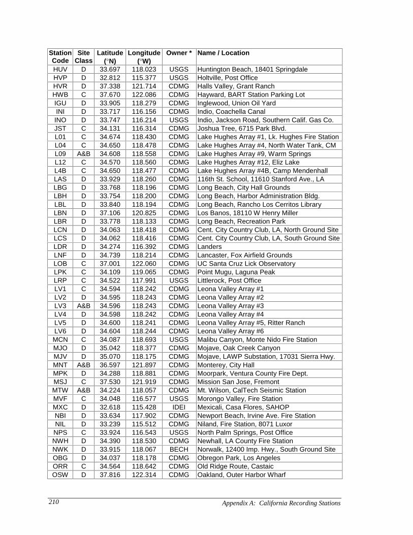
Appendix A: California Recording Stations210
StationCode
SiteClass
Latitude(°N)
Longitude(°W)
Owner * Name / Location
HUV D 33.697 118.023 USGS Huntington Beach, 18401 SpringdaleHVP D 32.812 115.377 USGS Holtville, Post OfficeHVR D 37.338 121.714 CDMG Halls Valley, Grant RanchHWB C 37.670 122.086 CDMG Hayward, BART Station Parking LotIGU D 33.905 118.279 CDMG Inglewood, Union Oil YardINI D 33.717 116.156 CDMG Indio, Coachella CanalINO D 33.747 116.214 USGS Indio, Jackson Road, Southern Calif. Gas Co.JST C 34.131 116.314 CDMG Joshua Tree, 6715 Park Blvd.L01 C 34.674 118.430 CDMG Lake Hughes Array #1, Lk. Hughes Fire StationL04 C 34.650 118.478 CDMG Lake Hughes Array #4, North Water Tank, CML09 A&B 34.608 118.558 CDMG Lake Hughes Array #9, Warm SpringsL12 C 34.570 118.560 CDMG Lake Hughes Array #12, Eliz LakeL4B C 34.650 118.477 CDMG Lake Hughes Array #4B, Camp MendenhallLAS D 33.929 118.260 CDMG 116th St. School, 11610 Stanford Ave., LALBG D 33.768 118.196 CDMG Long Beach, City Hall GroundsLBH D 33.754 118.200 CDMG Long Beach, Harbor Administration Bldg.LBL D 33.840 118.194 CDMG Long Beach, Rancho Los Cerritos LibraryLBN D 37.106 120.825 CDMG Los Banos, 18110 W Henry MillerLBR D 33.778 118.133 CDMG Long Beach, Recreation ParkLCN D 34.063 118.418 CDMG Cent. City Country Club, LA, North Ground SiteLCS D 34.062 118.416 CDMG Cent. City Country Club, LA, South Ground SiteLDR D 34.274 116.392 CDMG LandersLNF D 34.739 118.214 CDMG Lancaster, Fox Airfield GroundsLOB C 37.001 122.060 CDMG UC Santa Cruz Lick ObservatoryLPK C 34.109 119.065 CDMG Point Mugu, Laguna PeakLRP C 34.522 117.991 USGS Littlerock, Post OfficeLV1 C 34.594 118.242 CDMG Leona Valley Array #1LV2 D 34.595 118.243 CDMG Leona Valley Array #2LV3 A&B 34.596 118.243 CDMG Leona Valley Array #3LV4 D 34.598 118.242 CDMG Leona Valley Array #4LV5 D 34.600 118.241 CDMG Leona Valley Array #5, Ritter RanchLV6 D 34.604 118.244 CDMG Leona Valley Array #6MCN C 34.087 118.693 USGS Malibu Canyon, Monte Nido Fire StationMJO D 35.042 118.377 CDMG Mojave, Oak Creek CanyonMJV D 35.070 118.175 CDMG Mojave, LAWP Substation, 17031 Sierra Hwy.MNT A&B 36.597 121.897 CDMG Monterey, City HallMPK D 34.288 118.881 CDMG Moorpark, Ventura County Fire Dept.MSJ C 37.530 121.919 CDMG Mission San Jose, FremontMTW A&B 34.224 118.057 CDMG Mt. Wilson, CalTech Seismic StationMVF C 34.048 116.577 USGS Morongo Valley, Fire StationMXC D 32.618 115.428 IDEI Mexicali, Casa Flores, SAHOPNBI D 33.634 117.902 CDMG Newport Beach, Irvine Ave. Fire StationNIL D 33.239 115.512 CDMG Niland, Fire Station, 8071 LuxorNPS C 33.924 116.543 USGS North Palm Springs, Post OfficeNWH D 34.390 118.530 CDMG Newhall, LA County Fire StationNWK D 33.915 118.067 BECH Norwalk, 12400 Imp. Hwy., South Ground SiteOBG D 34.037 118.178 CDMG Obregon Park, Los AngelesORR C 34.564 118.642 CDMG Old Ridge Route, CastaicOSW D 37.816 122.314 CDMG Oakland, Outer Harbor Wharf

Appendix A: California Recording Stations 211
StationCode
SiteClass
Latitude(°N)
Longitude(°W)
Owner * Name / Location
PAS C 34.140 118.120 CIT Pasadena, CalTech AthenaeumPCD A&B 34.334 118.396 CDMG Pacioma Dam, DownstreamPDL C 34.578 118.113 USGS Palmdale, Fire StationPDS C 34.077 118.800 CDMG Point Dume School, MalibuPGS D 40.324 124.286 CDMG Petrolia, General StorePHN D 34.145 119.206 CDMG Port Hueneme, Navy Lab, Bldg. 570PHT A&B 37.790 122.429 CDMG Pacific Heights, 2150 California, San FranciscoPIE A&B 37.823 122.233 CDMG Piedmont, Jr. High School GroundsPKC C 34.288 118.375 CDMG Pacoima, Kagel Canyon, 12587 Dexter ParkPLC C 33.324 116.683 CDMG Puerta La Cruz, USFS Storage Bldg.PLS D 32.790 115.860 USGS Plaster CityPMG D 34.113 119.119 CDMG Point Mugu, Naval Air StationPPP C 34.508 117.522 OWNR Pearblossom, Pumping PlantPRD D 33.890 117.641 ACOE Prado Dam, DownstreamPRS C 37.792 122.457 CDMG San Francisco PresidioPSA D 33.829 116.501 CDMG Palm Springs, AirportPSL A&B 34.150 118.170 CIT Pasadena, Old CalTech Seismo LabPSW C 34.136 118.127 USGS NSMP Pasadena Laboratory, Ground StationPTB A&B 37.820 122.520 CDMG Point BonitaPTS C 32.929 115.699 USGS Parachute Test SitePVC A&B 33.746 118.396 CDMG Rancho Palos Verdes, Crestmont CollegePWS A&B 34.021 116.009 CDMG Twenty-Nine Palms, Pinto Wye StationRCH C 37.935 122.342 CDMG Richmond, City HallRDL C 40.503 124.100 CDMG Rio Dell, Painter St. OverpassRGR D 34.827 118.265 CDMG Rosamond, Godde RanchRHE C 33.787 118.356 CDMG Rolling Hills Estates, Rancho Vista SchoolRIN A&B 37.786 122.391 CDMG Rincon Hill, Fremont & Harrison, San FranciscoRNC C 34.104 117.574 CDMG Rancho Cucamonga, Law & Justice CenterROS D 34.870 118.206 CDMG Rosamond, AirportRVA C 33.951 117.446 CDMG Riverside Airport, Maintenance ShopSAG C 36.753 121.396 CDMG Sago South, Cienega Rd., HollisterSAL D 36.671 121.642 CDMG Salinas, John & Work St.SCP C 40.026 124.069 CDMG Shelter Cove, Power Plant YardSFG C 37.806 122.472 USGS Golden Gate Bridge, Toll Plaza, San FranciscoSFO D 37.622 122.398 CDMG San Francisco International AirportSFY D 34.236 118.439 CDMG Arleta, Nordhoff Fire StationSJB C 36.846 121.536 CDMG San Juan Bautista, Fire Station, 24 PolkSLA D 37.419 122.205 USGS Stanford Linear Accelerator CenterSMG D 34.011 118.490 CDMG Santa Monica, City Hall GroundsSNM D 34.115 118.130 CDMG San Marino, Southwestern AcademySOD C 34.156 117.675 ACOE San Antonio Dam, DownstreamSPC C 34.097 118.475 MWD Sepulveda Canyon, Spillway Building, LASPP C 33.722 118.309 CDMG San Pedro, Palos Verdes, 1414 W 25th
SSA A&B 34.231 118.713 DOE Canoga Park, Santa Susana (ETEC)SSF A&B 37.674 122.388 CDMG South San Francisco, Sierra PointSTG C 37.255 122.031 CDMG Saratoga, 14675 Aloha Ave.SUP C 32.955 115.823 USGS Superstition Mountain, Camera SiteSVL D 37.402 122.024 USGS Sunnyvale, 1058 Colton Ave.SYH D 34.326 118.444 CDMG Sylmar, County Hospital Parking Lot
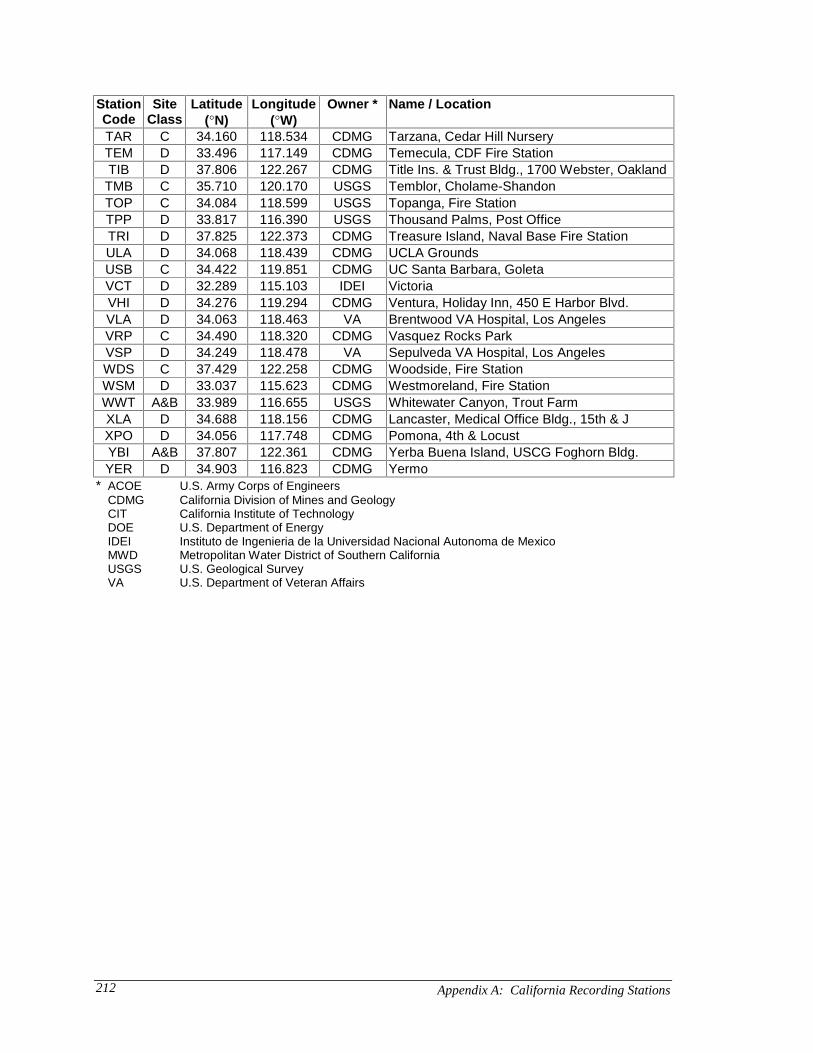
Appendix A: California Recording Stations212
StationCode
SiteClass
Latitude(°N)
Longitude(°W)
Owner * Name / Location
TAR C 34.160 118.534 CDMG Tarzana, Cedar Hill NurseryTEM D 33.496 117.149 CDMG Temecula, CDF Fire StationTIB D 37.806 122.267 CDMG Title Ins. & Trust Bldg., 1700 Webster, OaklandTMB C 35.710 120.170 USGS Temblor, Cholame-ShandonTOP C 34.084 118.599 USGS Topanga, Fire StationTPP D 33.817 116.390 USGS Thousand Palms, Post OfficeTRI D 37.825 122.373 CDMG Treasure Island, Naval Base Fire StationULA D 34.068 118.439 CDMG UCLA GroundsUSB C 34.422 119.851 CDMG UC Santa Barbara, GoletaVCT D 32.289 115.103 IDEI VictoriaVHI D 34.276 119.294 CDMG Ventura, Holiday Inn, 450 E Harbor Blvd.VLA D 34.063 118.463 VA Brentwood VA Hospital, Los AngelesVRP C 34.490 118.320 CDMG Vasquez Rocks ParkVSP D 34.249 118.478 VA Sepulveda VA Hospital, Los AngelesWDS C 37.429 122.258 CDMG Woodside, Fire StationWSM D 33.037 115.623 CDMG Westmoreland, Fire StationWWT A&B 33.989 116.655 USGS Whitewater Canyon, Trout FarmXLA D 34.688 118.156 CDMG Lancaster, Medical Office Bldg., 15th & JXPO D 34.056 117.748 CDMG Pomona, 4th & LocustYBI A&B 37.807 122.361 CDMG Yerba Buena Island, USCG Foghorn Bldg.YER D 34.903 116.823 CDMG Yermo
* ACOE U.S. Army Corps of EngineersCDMG California Division of Mines and GeologyCIT California Institute of TechnologyDOE U.S. Department of EnergyIDEI Instituto de Ingenieria de la Universidad Nacional Autonoma de MexicoMWD Metropolitan Water District of Southern CaliforniaUSGS U.S. Geological SurveyVA U.S. Department of Veteran Affairs

Appendix B: Data; Parametric Method 213
APPENDIX BDATA; PARAMETRIC METHOD
The statistics on normalized phase differences that are used in Chapter 3 are listed in
Table B.1. The station code is the same as in Table A.1, where the locations of all the
recording stations are tabulated. Source to site distances are taken from:
• Boore et al. (1993, 1994, 1997)• Chang et al. (1996)
and calculated using information on the seismogenic rupture in:
• Archuleta and Day (1980)• Bolt et al. (1985)• Bouchon (1982)• Chavez et al. (1982)• Hagerty and Schwartz (1996)• Hauksson et al. (1993)• Hauksson and Jones (1995)• Jones and Hauksson (1988)• Kanamori and Regan (1982)• Pacheco and Nabelek (1988)• Wald et al. (1991)• Whitcomb et al. (1973).
The parameters in Table B.1 are:
• D: The distance from the site to the vertical projection of the seismogenicrupture on the surface of the Earth.
• µL: The mean normalized phase difference for large Fourier amplitudes.
• σL
2: The variance of normalized phase difference for large Fourieramplitudes.
• µI: The mean normalized phase difference for intermediate Fourier
amplitudes.• σ
I2: The variance of normalized phase difference for intermediate Fourier
amplitudes.• µ
S: The mean normalized phase difference for small Fourier amplitudes.
• σS
2: The variance of normalized phase difference for small Fourieramplitudes.
• wu: The weight of the uniform distribution for small Fourier amplitudes.

Appendix B: Data; Parametric Method214
Table B.1: Statistics on normalized phase differences that are used in Chapter 3.Earthquake Station D (km) µL σL
2 µI σI2 µS σS
2 wuCoyote CYC 1.6 0.63 0.0033 0.63 0.0054 0.65 0.0044 0.009Lake G01 9.1 0.61 0.0007 0.62 0.0023 0.63 0.0081 0.027
G02 7.4 0.61 0.0011 0.62 0.0020 0.62 0.0056 0.018G03 5.3 0.60 0.0022 0.60 0.0061 0.62 0.0070 0.009G04 3.7 0.58 0.0068 0.59 0.0086 0.63 0.0072 0.009G06 1.2 0.63 0.0005 0.63 0.0040 0.64 0.0047 0.044HVR 30.0 0.54 0.0134 0.60 0.0245 0.60 0.0475 0.284SJB 17.9 0.51 0.0107 0.58 0.0121 0.61 0.0099 0.116
Whittier ALF 3.0 0.59 0.0007 0.60 0.0035 0.59 0.0065 0.018Narrows BHA 22.5 0.51 0.0106 0.52 0.0138 0.56 0.0159 0.089
CHC 64.4 0.40 0.0096 0.46 0.0233 0.55 0.0383 0.676DOW 11.3 0.54 0.0066 0.54 0.0126 0.57 0.0083 0.107ECP 10.5 0.59 0.0014 0.58 0.0069 0.61 0.0081 0.071FYP 35.5 0.54 0.0025 0.52 0.0160 0.55 0.0221 0.293H05 103.9 0.34 0.0088 0.37 0.0274 0.39 0.0269 0.338HBL 39.8 0.46 0.0165 0.49 0.0193 0.52 0.0143 0.151HSL 20.5 0.50 0.0073 0.53 0.0127 0.55 0.0167 0.116IGU 19.4 0.54 0.0032 0.53 0.0077 0.54 0.0093 0.071L01 71.7 0.43 0.0153 0.46 0.0211 0.55 0.0249 0.356LAS 16.4 0.55 0.0011 0.55 0.0050 0.56 0.0050 0.080LBH 30.2 0.44 0.0307 0.52 0.0216 0.56 0.0217 0.107LBL 20.9 0.52 0.0056 0.53 0.0085 0.55 0.0117 0.071LBR 26.6 0.45 0.0183 0.50 0.0180 0.56 0.0177 0.276LCN 27.7 0.50 0.0077 0.52 0.0118 0.55 0.0123 0.080LCS 27.5 0.58 0.0066 0.57 0.0170 0.62 0.0157 0.356LV5 58.6 0.44 0.0070 0.49 0.0184 0.55 0.0223 0.222LV6 59.1 0.51 0.0043 0.53 0.0159 0.57 0.0139 0.231MPK 73.9 0.37 0.0087 0.43 0.0348 0.60 0.0492 0.693NWH 51.0 0.53 0.0083 0.53 0.0206 0.60 0.0306 0.596OBG 5.6 0.58 0.0011 0.57 0.0058 0.57 0.0087 0.044ORR 71.5 0.39 0.0076 0.45 0.0336 0.57 0.0416 0.391PDS 62.9 0.41 0.0077 0.45 0.0185 0.57 0.0213 0.516PKC 32.9 0.51 0.0034 0.53 0.0130 0.55 0.0167 0.258RGR 83.8 0.38 0.0040 0.41 0.0202 0.49 0.0302 0.507RNC 43.9 0.46 0.0036 0.47 0.0112 0.47 0.0228 0.124RVA 56.2 0.48 0.0048 0.46 0.0080 0.48 0.0175 0.187SFY 34.1 0.48 0.0084 0.50 0.0138 0.55 0.0185 0.036SNM 3.8 0.61 0.0015 0.60 0.0039 0.61 0.0111 0.018SYH 40.4 0.45 0.0047 0.48 0.0169 0.53 0.0224 0.213TAR 39.3 0.48 0.0027 0.50 0.0064 0.50 0.0080 0.053VRP 48.9 0.48 0.0017 0.48 0.0063 0.50 0.0127 0.124XLA 67.4 0.41 0.0049 0.42 0.0209 0.49 0.0238 0.267XPO 28.0 0.50 0.0054 0.52 0.0140 0.52 0.0158 0.258
Morgan A01 53.5 0.30 0.0416 0.41 0.0338 0.49 0.0256 0.453Hill A1E 50.9 0.46 0.0299 0.51 0.0357 0.55 0.0372 0.667
AGW 24.4 0.37 0.0654 0.45 0.0292 0.46 0.0313 0.302CAP 40.1 0.49 0.0075 0.52 0.0137 0.51 0.0180 0.027CLS 24.6 0.51 0.0077 0.53 0.0107 0.55 0.0226 0.231CYC 1.0 0.60 0.0004 0.61 0.0019 0.63 0.0049 0.000

Appendix B: Data; Parametric Method 215
Earthquake Station D (km) µL σL2 µI σI
2 µS σS2 wu
Morgan G01 13.5 0.57 0.0021 0.59 0.0081 0.62 0.0105 0.080Hill G02 12.0 0.56 0.0067 0.58 0.0094 0.62 0.0115 0.009
G03 10.9 0.53 0.0156 0.59 0.0101 0.65 0.0051 0.044G04 8.7 0.54 0.0112 0.58 0.0123 0.62 0.0115 0.018G06 6.5 0.60 0.0026 0.64 0.0057 0.66 0.0063 0.053G07 8.4 0.56 0.0053 0.57 0.0107 0.63 0.0106 0.071GIL 13.3 0.60 0.0012 0.59 0.0060 0.62 0.0104 0.098HVR 2.4 0.49 0.0086 0.60 0.0125 0.65 0.0113 0.036LBN 60.5 0.40 0.0307 0.49 0.0512 0.61 0.0637 0.827LOB 46.7 0.55 0.0026 0.56 0.0140 0.55 0.0294 0.231MSJ 30.3 0.44 0.0319 0.48 0.0296 0.52 0.0432 0.711SFO 70.5 0.33 0.0206 0.41 0.0335 0.40 0.0269 0.480SJB 26.4 0.45 0.0255 0.58 0.0192 0.60 0.0347 0.436
Parkfield C02 6.6 0.59 0.0016 0.58 0.0095 0.61 0.0089 0.022C05 9.3 0.50 0.0022 0.51 0.0058 0.54 0.0078 0.000C08 13.0 0.54 0.0060 0.56 0.0102 0.58 0.0093 0.022TMB 16.1 0.60 0.0019 0.59 0.0050 0.61 0.0035 0.044
North Palm DSP 1.6 0.59 0.0020 0.60 0.0057 0.62 0.0062 0.089Springs H01 59.6 0.49 0.0013 0.49 0.0057 0.49 0.0186 0.053
H02 53.8 0.59 0.0022 0.58 0.0057 0.57 0.0160 0.133H03 48.1 0.63 0.0010 0.64 0.0030 0.63 0.0125 0.107H04 43.0 0.51 0.0040 0.51 0.0102 0.51 0.0156 0.187H05 39.4 0.50 0.0042 0.50 0.0170 0.51 0.0163 0.071H06 35.6 0.50 0.0144 0.52 0.0147 0.50 0.0173 0.133H08 27.8 0.54 0.0017 0.54 0.0097 0.57 0.0140 0.089H10 21.5 0.60 0.0010 0.59 0.0029 0.60 0.0119 0.107HES 70.6 0.39 0.0137 0.42 0.0345 0.44 0.0200 0.329INI 43.5 0.43 0.0230 0.51 0.0191 0.56 0.0192 0.196JST 22.7 0.51 0.0085 0.54 0.0163 0.59 0.0246 0.160LDR 31.4 0.53 0.0044 0.54 0.0089 0.57 0.0129 0.151PLC 68.2 0.44 0.0029 0.42 0.0122 0.43 0.0186 0.258PSA 12.0 0.52 0.0139 0.57 0.0090 0.60 0.0143 0.071RNC 81.0 0.39 0.0415 0.42 0.0341 0.45 0.0272 0.320RVA 68.6 0.42 0.0048 0.42 0.0094 0.43 0.0173 0.213TEM 69.5 0.40 0.0088 0.44 0.0171 0.49 0.0173 0.267
Imperial AEP 1.4 0.55 0.0012 0.57 0.0061 0.59 0.0089 0.089Valley AGR 1.0 0.50 0.0057 0.52 0.0102 0.55 0.0131 0.222
BCR 2.6 0.52 0.0053 0.55 0.0057 0.55 0.0130 0.036BRA 8.5 0.49 0.0069 0.47 0.0143 0.49 0.0146 0.204CAL 23.0 0.44 0.0286 0.44 0.0256 0.47 0.0247 0.169CC4 49.0 0.40 0.0101 0.46 0.0317 0.48 0.0376 0.444CHU 17.7 0.41 0.0206 0.49 0.0200 0.53 0.0208 0.089CMP 23.2 0.42 0.0276 0.47 0.0318 0.48 0.0271 0.204CPR 23.5 0.35 0.0569 0.41 0.0461 0.45 0.0227 0.382CUC 12.9 0.49 0.0096 0.51 0.0105 0.53 0.0095 0.071CXO 10.6 0.50 0.0098 0.50 0.0166 0.51 0.0103 0.107DLT 32.7 0.37 0.0782 0.39 0.0365 0.43 0.0198 0.356E01 22.0 0.44 0.0155 0.45 0.0150 0.49 0.0114 0.107E02 16.0 0.43 0.0017 0.44 0.0147 0.47 0.0122 0.044E03 11.2 0.48 0.0042 0.48 0.0154 0.50 0.0089 0.089

Appendix B: Data; Parametric Method216
Earthquake Station D (km) µL σL2 µI σI
2 µS σS2 wu
Imperial E04 6.8 0.53 0.0065 0.55 0.0082 0.58 0.0121 0.062Valley E05 4.0 0.53 0.0046 0.56 0.0042 0.59 0.0072 0.044
E06 1.3 0.53 0.0022 0.58 0.0046 0.60 0.0063 0.044E07 0.6 0.55 0.0028 0.55 0.0098 0.57 0.0130 0.053E08 3.8 0.53 0.0010 0.52 0.0035 0.55 0.0067 0.071E10 8.5 0.48 0.0070 0.48 0.0092 0.52 0.0114 0.080E11 12.6 0.46 0.0020 0.47 0.0096 0.50 0.0111 0.062E12 18.0 0.40 0.0148 0.45 0.0160 0.50 0.0140 0.080E13 22.0 0.44 0.0241 0.48 0.0188 0.49 0.0132 0.089EDA 5.1 0.52 0.0009 0.52 0.0103 0.56 0.0073 0.044ELC 6.2 0.49 0.0070 0.50 0.0117 0.55 0.0087 0.089HVP 7.5 0.50 0.0052 0.51 0.0091 0.53 0.0136 0.053MXC 8.4 0.56 0.0029 0.57 0.0095 0.57 0.0089 0.151NIL 36.0 0.46 0.0172 0.47 0.0240 0.47 0.0278 0.338PLS 32.0 0.50 0.0031 0.50 0.0109 0.51 0.0158 0.018PTS 14.0 0.44 0.0109 0.48 0.0161 0.52 0.0116 0.116SUP 26.0 0.49 0.0008 0.48 0.0087 0.51 0.0105 0.071VCT 43.5 0.36 0.0163 0.41 0.0375 0.44 0.0156 0.276WSM 15.0 0.48 0.0300 0.49 0.0197 0.54 0.0195 0.178
San GPK 21.1 0.51 0.0030 0.55 0.0106 0.58 0.0147 0.107Fernando L01 23.4 0.55 0.0161 0.56 0.0248 0.61 0.0164 0.222
L09 20.2 0.64 0.0016 0.63 0.0036 0.63 0.0135 0.107L12 17.0 0.63 0.0051 0.61 0.0095 0.61 0.0120 0.089PAS 25.7 0.46 0.0081 0.49 0.0085 0.52 0.0128 0.044PDL 28.6 0.55 0.0119 0.57 0.0173 0.60 0.0123 0.107PPP 37.4 0.58 0.0052 0.58 0.0158 0.60 0.0138 0.204PSL 21.9 0.56 0.0056 0.55 0.0126 0.57 0.0117 0.178SOD 70.0 0.53 0.0061 0.54 0.0155 0.53 0.0157 0.222
Northridge ALF 37.2 0.39 0.0100 0.46 0.0231 0.50 0.0190 0.133ANB 48.6 0.47 0.0053 0.49 0.0182 0.56 0.0236 0.258ANI 73.2 0.39 0.0062 0.42 0.0278 0.41 0.0306 0.320ANV 39.4 0.37 0.0099 0.42 0.0254 0.54 0.0238 0.196BAD 65.6 0.40 0.0051 0.42 0.0217 0.48 0.0192 0.169BHA 30.8 0.42 0.0124 0.47 0.0127 0.48 0.0108 0.044CMO 44.3 0.43 0.0437 0.45 0.0253 0.51 0.0286 0.302DOW 47.4 0.37 0.0192 0.42 0.0230 0.45 0.0144 0.151ELZ 38.1 0.40 0.0041 0.42 0.0149 0.51 0.0197 0.169FYP 82.7 0.33 0.0055 0.38 0.0311 0.37 0.0360 0.569GPK 24.4 0.49 0.0068 0.53 0.0102 0.56 0.0115 0.124HBL 78.3 0.36 0.0339 0.41 0.0269 0.48 0.0364 0.516HSL 24.8 0.47 0.0041 0.50 0.0140 0.52 0.0110 0.089HUV 73.9 0.38 0.0070 0.44 0.0218 0.44 0.0200 0.267IGU 43.1 0.38 0.0186 0.44 0.0229 0.47 0.0131 0.231L01 37.7 0.45 0.0129 0.53 0.0240 0.53 0.0149 0.373L09 28.4 0.53 0.0008 0.53 0.0104 0.57 0.0090 0.124L4B 34.0 0.48 0.0022 0.49 0.0140 0.53 0.0155 0.178L04 34.0 0.48 0.0026 0.49 0.0129 0.54 0.0166 0.160LAS 42.0 0.40 0.0133 0.42 0.0224 0.41 0.0170 0.178LBL 52.7 0.39 0.0413 0.43 0.0288 0.44 0.0172 0.160LCN 24.4 0.47 0.0068 0.50 0.0140 0.54 0.0082 0.116
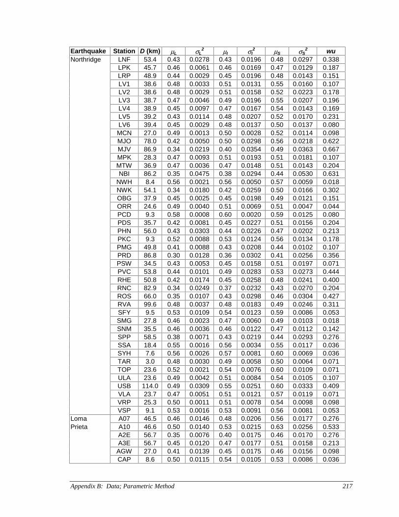
Appendix B: Data; Parametric Method 217
Earthquake Station D (km) µL σL2 µI σI
2 µS σS2 wu
Northridge LNF 53.4 0.43 0.0278 0.43 0.0196 0.48 0.0297 0.338LPK 45.7 0.46 0.0061 0.46 0.0169 0.47 0.0129 0.187LRP 48.9 0.44 0.0029 0.45 0.0196 0.48 0.0143 0.151LV1 38.6 0.48 0.0033 0.51 0.0131 0.55 0.0160 0.107LV2 38.6 0.48 0.0029 0.51 0.0158 0.52 0.0223 0.178LV3 38.7 0.47 0.0046 0.49 0.0196 0.55 0.0207 0.196LV4 38.9 0.45 0.0097 0.47 0.0167 0.54 0.0143 0.169LV5 39.2 0.43 0.0114 0.48 0.0207 0.52 0.0170 0.231LV6 39.4 0.45 0.0029 0.48 0.0137 0.50 0.0137 0.080MCN 27.0 0.49 0.0013 0.50 0.0028 0.52 0.0114 0.098MJO 78.0 0.42 0.0050 0.50 0.0298 0.56 0.0218 0.622MJV 86.9 0.34 0.0219 0.40 0.0354 0.49 0.0363 0.667MPK 28.3 0.47 0.0093 0.51 0.0193 0.51 0.0181 0.107MTW 36.9 0.47 0.0036 0.47 0.0148 0.51 0.0143 0.204NBI 86.2 0.35 0.0475 0.38 0.0294 0.44 0.0530 0.631
NWH 8.4 0.56 0.0021 0.56 0.0050 0.57 0.0059 0.018NWK 54.1 0.34 0.0180 0.42 0.0259 0.50 0.0166 0.302OBG 37.9 0.45 0.0025 0.45 0.0198 0.49 0.0121 0.151ORR 24.6 0.49 0.0040 0.51 0.0069 0.51 0.0047 0.044PCD 9.3 0.58 0.0008 0.60 0.0020 0.59 0.0125 0.080PDS 35.7 0.42 0.0081 0.45 0.0227 0.51 0.0156 0.204PHN 56.0 0.43 0.0303 0.44 0.0226 0.47 0.0202 0.213PKC 9.3 0.52 0.0088 0.53 0.0124 0.56 0.0134 0.178PMG 49.8 0.41 0.0088 0.43 0.0208 0.44 0.0102 0.107PRD 86.8 0.30 0.0128 0.36 0.0302 0.41 0.0256 0.356PSW 34.5 0.43 0.0053 0.45 0.0158 0.51 0.0197 0.071PVC 53.8 0.44 0.0101 0.49 0.0283 0.53 0.0273 0.444RHE 50.8 0.42 0.0174 0.45 0.0258 0.48 0.0241 0.400RNC 82.9 0.34 0.0249 0.37 0.0232 0.43 0.0270 0.204ROS 66.0 0.35 0.0107 0.43 0.0298 0.46 0.0304 0.427RVA 99.6 0.48 0.0037 0.48 0.0183 0.49 0.0246 0.311SFY 9.5 0.53 0.0109 0.54 0.0123 0.59 0.0086 0.053SMG 27.8 0.46 0.0023 0.47 0.0060 0.49 0.0103 0.018SNM 35.5 0.46 0.0036 0.46 0.0122 0.47 0.0112 0.142SPP 58.5 0.38 0.0071 0.43 0.0219 0.44 0.0293 0.276SSA 18.4 0.55 0.0016 0.56 0.0034 0.55 0.0117 0.036SYH 7.6 0.56 0.0026 0.57 0.0081 0.60 0.0069 0.036TAR 3.0 0.48 0.0030 0.49 0.0058 0.50 0.0064 0.071TOP 23.6 0.52 0.0021 0.54 0.0076 0.60 0.0109 0.071ULA 23.6 0.49 0.0042 0.51 0.0084 0.54 0.0105 0.107USB 114.0 0.49 0.0309 0.55 0.0251 0.60 0.0333 0.409VLA 23.7 0.47 0.0051 0.51 0.0121 0.57 0.0119 0.071VRP 25.3 0.50 0.0011 0.51 0.0078 0.54 0.0098 0.098VSP 9.1 0.53 0.0016 0.53 0.0091 0.56 0.0081 0.053
Loma A07 46.5 0.46 0.0146 0.48 0.0206 0.56 0.0177 0.276Prieta A10 46.6 0.50 0.0140 0.53 0.0215 0.63 0.0256 0.533
A2E 56.7 0.35 0.0076 0.40 0.0175 0.46 0.0170 0.276A3E 56.7 0.45 0.0120 0.47 0.0177 0.51 0.0158 0.213AGW 27.0 0.41 0.0139 0.45 0.0175 0.46 0.0156 0.098CAP 8.6 0.50 0.0115 0.54 0.0105 0.53 0.0086 0.036

Appendix B: Data; Parametric Method218
Earthquake Station D (km) µL σL2 µI σI
2 µS σS2 wu
Loma CFH 83.5 0.41 0.0043 0.45 0.0223 0.57 0.0280 0.427Prieta CLS 0.0 0.58 0.0046 0.59 0.0092 0.59 0.0076 0.044
CYC 21.7 0.53 0.0027 0.52 0.0158 0.55 0.0133 0.196DMH 75.9 0.42 0.0026 0.42 0.0159 0.51 0.0353 0.356EMV 81.0 0.38 0.0123 0.42 0.0144 0.44 0.0218 0.156FMS 42.4 0.38 0.0096 0.43 0.0178 0.46 0.0130 0.111G01 10.5 0.60 0.0005 0.60 0.0029 0.61 0.0093 0.018G02 12.1 0.56 0.0046 0.57 0.0088 0.60 0.0113 0.053G03 14.0 0.54 0.0032 0.56 0.0080 0.60 0.0090 0.044G04 15.8 0.51 0.0112 0.52 0.0145 0.56 0.0164 0.071G06 19.9 0.54 0.0063 0.56 0.0129 0.60 0.0109 0.151G07 24.3 0.51 0.0063 0.52 0.0124 0.54 0.0057 0.080GIL 10.9 0.60 0.0005 0.59 0.0037 0.60 0.0102 0.036GOF 12.3 0.55 0.0085 0.53 0.0174 0.56 0.0137 0.124HAD 25.4 0.47 0.0076 0.51 0.0114 0.56 0.0105 0.022HCH 27.8 0.47 0.0067 0.50 0.0138 0.58 0.0113 0.133HVR 29.3 0.43 0.0092 0.45 0.0174 0.50 0.0175 0.320HWB 57.7 0.35 0.0047 0.38 0.0167 0.45 0.0127 0.213LOB 12.5 0.48 0.0027 0.49 0.0108 0.50 0.0123 0.142MNT 42.7 0.44 0.0046 0.45 0.0198 0.48 0.0228 0.311MSJ 42.0 0.43 0.0131 0.45 0.0225 0.44 0.0122 0.204OSW 78.8 0.38 0.0044 0.39 0.0099 0.39 0.0189 0.151PHT 80.5 0.39 0.0083 0.40 0.0211 0.45 0.0309 0.480PIE 77.2 0.44 0.0071 0.44 0.0099 0.47 0.0268 0.213PRS 82.0 0.40 0.0024 0.42 0.0202 0.52 0.0248 0.418PTB 87.5 0.43 0.0059 0.45 0.0265 0.57 0.0275 0.587RCH 92.0 0.36 0.0102 0.39 0.0151 0.44 0.0252 0.284RIN 78.5 0.41 0.0067 0.41 0.0108 0.46 0.0230 0.302SAG 34.1 0.48 0.0130 0.52 0.0272 0.59 0.0270 0.356SAL 31.4 0.42 0.0211 0.47 0.0170 0.51 0.0208 0.249SFG 84.0 0.40 0.0050 0.43 0.0258 0.41 0.0198 0.267SLA 35.0 0.44 0.0033 0.44 0.0135 0.49 0.0187 0.089SSF 67.6 0.45 0.0028 0.42 0.0072 0.44 0.0184 0.124SVL 27.5 0.41 0.0084 0.45 0.0110 0.47 0.0108 0.067TIB 76.3 0.34 0.0121 0.45 0.0254 0.43 0.0166 0.222TRI 81.5 0.37 0.0031 0.39 0.0090 0.36 0.0143 0.116
WDS 38.7 0.54 0.0115 0.51 0.0237 0.53 0.0286 0.382YBI 79.5 0.42 0.0028 0.40 0.0112 0.45 0.0196 0.302
Petrolia ERB 1.9 0.57 0.0071 0.54 0.0268 0.56 0.0227 0.302ERC 9.8 0.51 0.0043 0.50 0.0212 0.50 0.0159 0.124ERF 14.6 0.48 0.0125 0.50 0.0280 0.52 0.0206 0.142ERL 17.6 0.46 0.0105 0.51 0.0126 0.52 0.0112 0.062ERR 23.9 0.42 0.0132 0.44 0.0209 0.49 0.0147 0.356ERU 27.8 0.45 0.0082 0.37 0.0154 0.35 0.0138 0.071EUR 35.8 0.42 0.0150 0.45 0.0170 0.47 0.0207 0.356FER 10.0 0.48 0.0102 0.52 0.0202 0.52 0.0088 0.169FRT 13.7 0.45 0.0125 0.46 0.0331 0.46 0.0217 0.258PGS 0.0 0.59 0.0094 0.56 0.0163 0.56 0.0188 0.169RDL 12.3 0.53 0.0045 0.52 0.0226 0.54 0.0142 0.062SCP 32.6 0.36 0.0294 0.36 0.0340 0.40 0.0362 0.356

Appendix C: Data; Method of Envelopes 219
APPENDIX CDATA; METHOD OF ENVELOPES
The statistics on whitened intensity functions that are used in Chapter 4 are listed in
Table C.1. The station code is the same as in Table A.1, where the locations of all the
recording stations are tabulated. Source to site distances are taken from:
• Boore et al. (1993, 1994, 1997)• Chang et al. (1996)
and calculated using information on the seismogenic rupture in:
• Archuleta and Day (1980)• Bolt et al. (1985)• Bouchon (1982)• Chavez et al. (1982)• Hagerty and Schwartz (1996)• Hauksson et al. (1993)• Hauksson and Jones (1995)• Jones and Hauksson (1988)• Kanamori and Regan (1982)• Pacheco and Nabelek (1988)• Wald et al. (1991)• Whitcomb et al. (1973).
The parameters in Table C.1 are:
• D: The distance from the site to the vertical projection of the seismogenic
rupture on the surface of the Earth.
• γ0: The zeroth moment of the whitened intensity function about the origin
(i.e., the area under the whitened intensity function).
• γ1: The first moment of the whitened intensity function about the origin.
• γ2: The second moment of the whitened intensity function about the
origin.

Appendix C: Data; Method of Envelopes220
Table C.1: The whitened intensity moments that are used in Chapter 4.Earthquake Station D (km) γ
0γ
1 (sec) γ
2 (sec2)
Coyote CYC 1.6 0.03764 0.1048 0.559Lake G01 9.1 0.03755 0.1325 0.941
G02 7.4 0.03662 0.1240 0.565G03 5.3 0.03673 0.1321 0.678G04 3.7 0.03727 0.1385 0.821G06 1.2 0.03818 0.1118 0.679HVR 30.0 0.04462 0.4059 8.684SJB 17.9 0.03659 0.1896 1.715
Whittier ALF 3.0 0.03630 0.1612 0.941Narrows BHA 22.5 0.03746 0.2630 2.829
CHC 64.4 0.03731 0.4957 10.095DOW 11.3 0.03810 0.2525 2.386ECP 10.5 0.03749 0.1786 1.336FYP 35.5 0.03760 0.3296 5.079H05 103.9 0.03756 0.5799 10.784HBL 39.8 0.03766 0.3919 5.815HSL 20.5 0.03740 0.2757 3.063IGU 19.4 0.03605 0.2489 2.194L01 71.7 0.03879 0.4514 8.104LAS 16.4 0.03728 0.2342 1.807LBH 30.2 0.03790 0.3468 5.570LBL 20.9 0.03673 0.2530 2.263LBR 26.6 0.03740 0.3774 5.960LCN 27.7 0.03746 0.2937 3.147LCS 27.5 0.03827 0.3273 6.309LV5 58.6 0.03853 0.3780 5.794LV6 59.1 0.03819 0.2989 4.306MPK 73.9 0.03803 0.5893 13.103NWH 51.0 0.03813 0.4386 8.896OBG 5.6 0.03730 0.2011 1.423ORR 71.5 0.03846 0.5051 10.422PDS 62.9 0.03816 0.4627 8.466PKC 32.9 0.03682 0.3326 4.896RGR 83.8 0.03743 0.5030 9.049RNC 43.9 0.03759 0.3939 5.166RVA 56.2 0.03656 0.3827 4.935SFY 34.1 0.03779 0.2992 3.383SNM 3.8 0.03729 0.1527 0.995SYH 40.4 0.03721 0.3717 5.474TAR 39.3 0.03671 0.3170 3.157VRP 48.9 0.03765 0.3372 3.534XLA 67.4 0.03717 0.4287 6.779XPO 28.0 0.03731 0.3279 4.082
Morgan A01 53.5 0.03679 0.5461 10.743Hill A1E 50.9 0.03895 0.5231 11.631
AGW 24.4 0.03753 0.5323 10.516CAP 40.1 0.03708 0.3131 3.541CLS 24.6 0.03779 0.3229 4.505
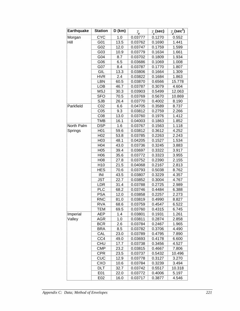
Appendix C: Data; Method of Envelopes 221
Earthquake Station D (km) γ0
γ1 (sec) γ
2 (sec2)
Morgan CYC 1.0 0.03777 0.1270 0.552Hill G01 13.5 0.03762 0.1690 1.441
G02 12.0 0.03747 0.1759 1.599G03 10.9 0.03779 0.1634 1.661G04 8.7 0.03702 0.1809 1.934G06 6.5 0.03686 0.1069 1.008G07 8.4 0.03787 0.1770 1.807GIL 13.3 0.03806 0.1664 1.309HVR 2.4 0.03822 0.1684 1.863LBN 60.5 0.03870 0.6566 15.778LOB 46.7 0.03787 0.3079 4.604MSJ 30.3 0.03903 0.5499 12.063SFO 70.5 0.03769 0.5670 10.869SJB 26.4 0.03770 0.4002 8.190
Parkfield C02 6.6 0.04705 0.3589 8.737C05 9.3 0.03812 0.2759 2.266C08 13.0 0.03760 0.1976 1.412TMB 16.1 0.04003 0.1863 1.852
North Palm DSP 1.6 0.03767 0.1563 1.118Springs H01 59.6 0.03812 0.3612 4.252
H02 53.8 0.03785 0.2263 2.243H03 48.1 0.04205 0.1527 1.534H04 43.0 0.03736 0.3245 3.883H05 39.4 0.03697 0.3322 3.917H06 35.6 0.03772 0.3323 3.955H08 27.8 0.03752 0.2390 2.155H10 21.5 0.04068 0.2167 2.813HES 70.6 0.03793 0.5038 8.762INI 43.5 0.03807 0.3229 4.357JST 22.7 0.03852 0.3004 4.767LDR 31.4 0.03788 0.2725 2.989PLC 68.2 0.03746 0.4484 6.388PSA 12.0 0.03858 0.2257 2.273RNC 81.0 0.03819 0.4990 8.827RVA 68.6 0.03759 0.4547 6.522TEM 69.5 0.03760 0.4315 6.745
Imperial AEP 1.4 0.03801 0.1931 1.261Valley AGR 1.0 0.03811 0.2874 2.858
BCR 2.6 0.03784 0.2467 1.965BRA 8.5 0.03782 0.3706 4.490CAL 23.0 0.03789 0.4795 7.890CC4 49.0 0.03693 0.4178 6.600CHU 17.7 0.03738 0.3456 4.527CMP 23.2 0.03815 0.4667 7.806CPR 23.5 0.03737 0.5432 10.496CUC 12.9 0.03778 0.3127 3.270CXO 10.6 0.03784 0.3239 3.494DLT 32.7 0.03742 0.5517 10.318E01 22.0 0.03772 0.4006 5.197E02 16.0 0.03717 0.3877 4.546

Appendix C: Data; Method of Envelopes222
Earthquake Station D (km) γ0
γ1 (sec) γ
2 (sec2)
Imperial E03 11.2 0.03774 0.3396 3.619Valley E04 6.8 0.03724 0.2167 1.745
E05 4.0 0.03721 0.2273 2.148E06 1.3 0.03826 0.2011 1.587E07 0.6 0.03777 0.2255 1.902E08 3.8 0.03730 0.2721 2.238E10 8.5 0.03757 0.3229 3.370E11 12.6 0.03777 0.3451 3.627E12 18.0 0.03778 0.3755 4.708E13 22.0 0.03795 0.3731 4.646EDA 5.1 0.03762 0.2546 2.106ELC 6.2 0.03821 0.2993 2.985HVP 7.5 0.03811 0.3016 2.903MXC 8.4 0.03859 0.2054 1.537NIL 36.0 0.03819 0.4669 8.193PLS 32.0 0.03769 0.3004 2.795PTS 14.0 0.03726 0.3451 4.106SUP 26.0 0.03741 0.3244 3.204VCT 43.5 0.03747 0.5291 9.203WSM 15.0 0.03793 0.3621 5.222
San GPK 21.1 0.03988 0.2465 2.639Fernando L01 23.4 0.03934 0.2408 3.425
L04 19.6 0.03907 0.2018 1.913L09 20.2 0.04201 0.1411 1.307L12 17.0 0.03867 0.1518 1.196PAS 25.7 0.03768 0.3235 3.251PDL 28.6 0.03870 0.2321 2.641PPP 37.4 0.03953 0.2045 1.988PSL 21.9 0.03848 0.2523 2.840SOD 70.0 0.03780 0.2947 3.251
Northridge ALF 37.2 0.03825 0.4324 6.402ANB 48.6 0.03883 0.4014 7.015ANI 73.2 0.03817 0.5231 9.541BHA 30.8 0.03851 0.3859 4.646CMO 44.3 0.04672 0.6799 16.474DOW 47.4 0.03797 0.4864 7.408FYP 82.7 0.03793 0.6174 12.575HBL 78.3 0.03910 0.6234 13.445HSL 24.8 0.03733 0.3042 3.048IGU 43.1 0.03851 0.4671 7.216L01 37.7 0.03733 0.3585 5.457L04 34.0 0.03811 0.3137 3.638L09 28.4 0.03825 0.2483 2.244L4B 34.0 0.03906 0.3620 4.831LAS 42.0 0.03847 0.5065 8.012LBG 58.7 0.03859 0.5965 12.197LBL 52.7 0.03884 0.5238 8.702LCN 24.4 0.03801 0.3130 3.254LNF 53.4 0.03822 0.5150 9.566LPK 45.7 0.03656 0.3759 4.703

Appendix C: Data; Method of Envelopes 223
Earthquake Station D (km) γ0
γ1 (sec) γ
2 (sec2)
Northridge LV1 38.6 0.03914 0.3474 4.537LV2 38.6 0.03880 0.3587 4.880LV3 38.7 0.03854 0.3731 5.341LV4 38.9 0.03832 0.3578 4.593LV5 39.2 0.03804 0.3909 5.721LV6 39.4 0.03804 0.3706 4.506MJO 78.0 0.03927 0.4673 9.395MJV 86.9 0.03749 0.6361 14.424MPK 28.3 0.03759 0.3387 4.229MTW 36.9 0.03841 0.3472 4.108NBI 86.2 0.03907 0.7104 16.557
NWH 8.4 0.03833 0.2272 1.661OBG 37.9 0.03776 0.3925 4.926ORR 24.6 0.03880 0.3030 2.672PCD 9.3 0.03750 0.1731 1.148PDS 35.7 0.03850 0.4080 5.628PHN 56.0 0.03810 0.4791 8.256PKC 9.3 0.03813 0.2866 3.591PMG 49.8 0.03741 0.4401 5.908PVC 53.8 0.03828 0.4803 9.032RHE 50.8 0.03836 0.4987 9.232RNC 82.9 0.03867 0.5476 9.347ROS 66.0 0.03809 0.5536 10.743RVA 99.6 0.03879 0.4527 7.717SFY 9.5 0.03831 0.2202 1.806SMG 27.8 0.03761 0.3470 3.557SNM 35.5 0.03684 0.3643 4.329SPP 58.5 0.03728 0.5139 9.024SYH 7.6 0.03798 0.1978 1.647TAR 3.0 0.03763 0.3072 2.834ULA 23.6 0.03805 0.2822 2.723USB 114.0 0.04358 0.5553 14.366VHI 62.4 0.03794 0.6571 14.871VRP 25.3 0.03805 0.3050 2.892
Loma A02 47.2 0.04519 0.6247 16.888Prieta A07 46.5 0.03882 0.3693 5.677
A10 46.6 0.03949 0.5221 12.216A2E 56.7 0.03832 0.4970 7.943A3E 56.7 0.03890 0.4039 5.802AGW 27.0 0.03847 0.4462 6.422CAP 8.6 0.03818 0.2724 2.393CFH 83.5 0.03818 0.4102 6.945CLS 0.0 0.03723 0.1782 1.272CYC 21.7 0.03743 0.2889 3.387DMH 75.9 0.03860 0.4896 8.534EMV 81.0 0.03803 0.5588 12.015FMS 42.4 0.03824 0.5517 11.798G01 10.5 0.03739 0.1640 1.024G02 12.1 0.03782 0.1982 1.644G03 14.0 0.03781 0.2105 1.636

Appendix C: Data; Method of Envelopes224
Earthquake Station D (km) γ0
γ1 (sec) γ
2 (sec2)
Loma G04 15.8 0.03765 0.2816 3.247Prieta G06 19.9 0.03729 0.2267 2.632
G07 24.3 0.03762 0.2805 2.664GIL 10.9 0.03732 0.1696 1.136
GOF 12.3 0.03748 0.2649 2.802HAD 25.4 0.03760 0.4010 8.736HCH 27.8 0.03793 0.4282 9.703HSP 28.2 0.04005 0.3833 6.854HVR 29.3 0.03829 0.4248 6.581HWB 57.7 0.03714 0.4658 6.723LOB 12.5 0.03773 0.3212 3.257MNT 42.7 0.03777 0.4464 7.097MSJ 42.0 0.03804 0.4692 7.432OSW 78.8 0.03775 0.4806 7.043PHT 80.5 0.03861 0.5420 10.409PIE 77.2 0.03870 0.4630 7.405PRS 82.0 0.03829 0.4704 8.144PTB 87.5 0.03956 0.5001 9.802RCH 92.0 0.03698 0.4792 7.810RIN 78.5 0.03875 0.4285 6.119SAG 34.1 0.03948 0.4367 9.039SAL 31.4 0.03784 0.4702 8.674SFG 84.0 0.04368 0.6797 16.635SLA 35.0 0.03840 0.5392 11.707SSF 67.6 0.03778 0.4283 5.625STG 11.7 0.03828 0.2904 2.630SVL 27.5 0.03895 0.5100 9.806TIB 76.3 0.03787 0.4424 6.408TRI 81.5 0.03784 0.5061 7.648
WDS 38.7 0.03922 0.3813 6.317YBI 79.5 0.03900 0.4944 7.787
Petrolia ERB 1.9 0.03828 0.3016 4.037ERC 9.8 0.03766 0.3330 3.704ERF 14.6 0.03757 0.3273 3.897ERL 17.6 0.03739 0.3059 3.040ERR 23.9 0.03762 0.3946 5.266ERU 27.8 0.03686 0.4882 7.078EUR 35.8 0.03830 0.5010 9.013FER 10.0 0.03679 0.2949 3.063RDL 12.3 0.03796 0.3015 3.480SCP 32.6 0.03731 0.5889 11.205
Landers AMB 68.3 0.04158 0.8813 22.452BKR 88.3 0.03855 0.8169 19.526BRN 92.4 0.03882 0.8318 20.751BRS 37.7 0.03826 0.6832 14.166DSP 22.5 0.03796 0.6400 14.807FFP 45.4 0.03738 0.6442 13.823FTI 65.0 0.03813 0.7585 16.313FVR 25.8 0.03765 0.5869 13.071H05 69.1 0.03805 0.8063 20.220

Appendix C: Data; Method of Envelopes 225
Earthquake Station D (km) γ0
γ1 (sec) γ
2 (sec2)
Landers H10 51.3 0.03838 0.6584 14.717INI 54.9 0.03890 0.6122 14.189INO 49.6 0.03756 0.7385 18.783JST 11.3 0.03782 0.4625 9.118MVF 17.7 0.03856 0.6070 13.136NPS 27.7 0.03880 0.7248 17.477PLC 95.0 0.03808 0.9418 26.931PSA 36.7 0.03818 0.6998 16.761PWS 41.9 0.03839 0.6554 14.696RVA 95.9 0.03827 0.7817 18.503TPP 37.7 0.03759 0.7072 17.390
WWT 27.6 0.03785 0.7020 16.788YER 26.3 0.03812 0.6813 14.626


Appendix D: Data; Fourier Amplitudes 227
APPENDIX DDATA; FOURIER AMPLITUDES
The statistics on Fourier amplitude spectra that are used in Chapter 5 are listed in Table
D.1. The station code is the same as in Table A.1, where the locations of all the recording
stations are tabulated. Source to site distances are taken from:
• Boore et al. (1993, 1994, 1997)• Chang et al. (1996)
and calculated using information on the seismogenic rupture in:
• Archuleta and Day (1980)• Bolt et al. (1985)• Bouchon (1982)• Chavez et al. (1982)• Hagerty and Schwartz (1996)• Hauksson et al. (1993)• Hauksson and Jones (1995)• Jones and Hauksson (1988)• Kanamori and Regan (1982)• Pacheco and Nabelek (1988)• Wald et al. (1991)• Whitcomb et al. (1973).
The parameters in Table D.1 are:
• D: The distance from the site to the vertical projection of the seismogenic
rupture on the surface of the Earth.
• E: The sum of the squared Fourier amplitudes. Note that the values in
Table D.1 have not been normalized by N, the order of the Fourier
transform.
• MF: The central frequency parameter.
• VF: The spectral bandwidth parameter.

Appendix D: Data; Fourier Amplitudes228
Table D.1: The Fourier spectra parameters that are used in Chapter 5.Earthquake Station D (km) E (g2) MF VF
Coyote CYC 1.6 1194 0.105 0.00433Lake G01 9.1 268 0.265 0.03475
G02 7.4 1705 0.140 0.01369G03 5.3 1283 0.134 0.01391G04 3.7 1663 0.094 0.00556G06 1.2 2275 0.130 0.00481HVR 30.0 70 0.122 0.00690SJB 17.9 327 0.107 0.00594
Whittier ALF 3.0 2901 0.218 0.01686Narrows BHA 22.5 886 0.168 0.01243
CHC 64.4 94 0.129 0.00691DOW 11.3 771 0.157 0.01967ECP 10.5 617 0.256 0.02255FYP 35.5 236 0.146 0.00474H05 103.9 52 0.277 0.02056HBL 39.8 97 0.198 0.01599HSL 20.5 530 0.193 0.02117IGU 19.4 1119 0.174 0.02236L01 71.7 48 0.149 0.01158LAS 16.4 2902 0.214 0.01075LBH 30.2 286 0.108 0.00906LBL 20.9 1223 0.128 0.00871LBR 26.6 197 0.142 0.01360LCN 27.7 506 0.187 0.01523LCS 27.5 214 0.149 0.01085LV5 58.6 88 0.178 0.01296LV6 59.1 91 0.233 0.02010MPK 73.9 113 0.137 0.00569NWH 51.0 147 0.141 0.00675OBG 5.6 4192 0.222 0.01287ORR 71.5 288 0.119 0.00428PDS 62.9 82 0.163 0.00987PKC 32.9 631 0.165 0.00882RGR 83.8 106 0.149 0.00588RNC 43.9 128 0.400 0.04841RVA 56.2 97 0.313 0.03564SFY 34.1 335 0.153 0.01356SNM 3.8 994 0.202 0.02754SYH 40.4 197 0.167 0.01182TAR 39.3 8041 0.160 0.01009VRP 48.9 92 0.322 0.03457XLA 67.4 154 0.179 0.00957XPO 28.0 112 0.224 0.02565
Morgan A01 53.5 224 0.113 0.00690Hill A1E 50.9 61 0.115 0.00795
AGW 24.4 172 0.066 0.00438CAP 40.1 791 0.150 0.00854CLS 24.6 317 0.091 0.00445CYC 1.0 12816 0.121 0.01236
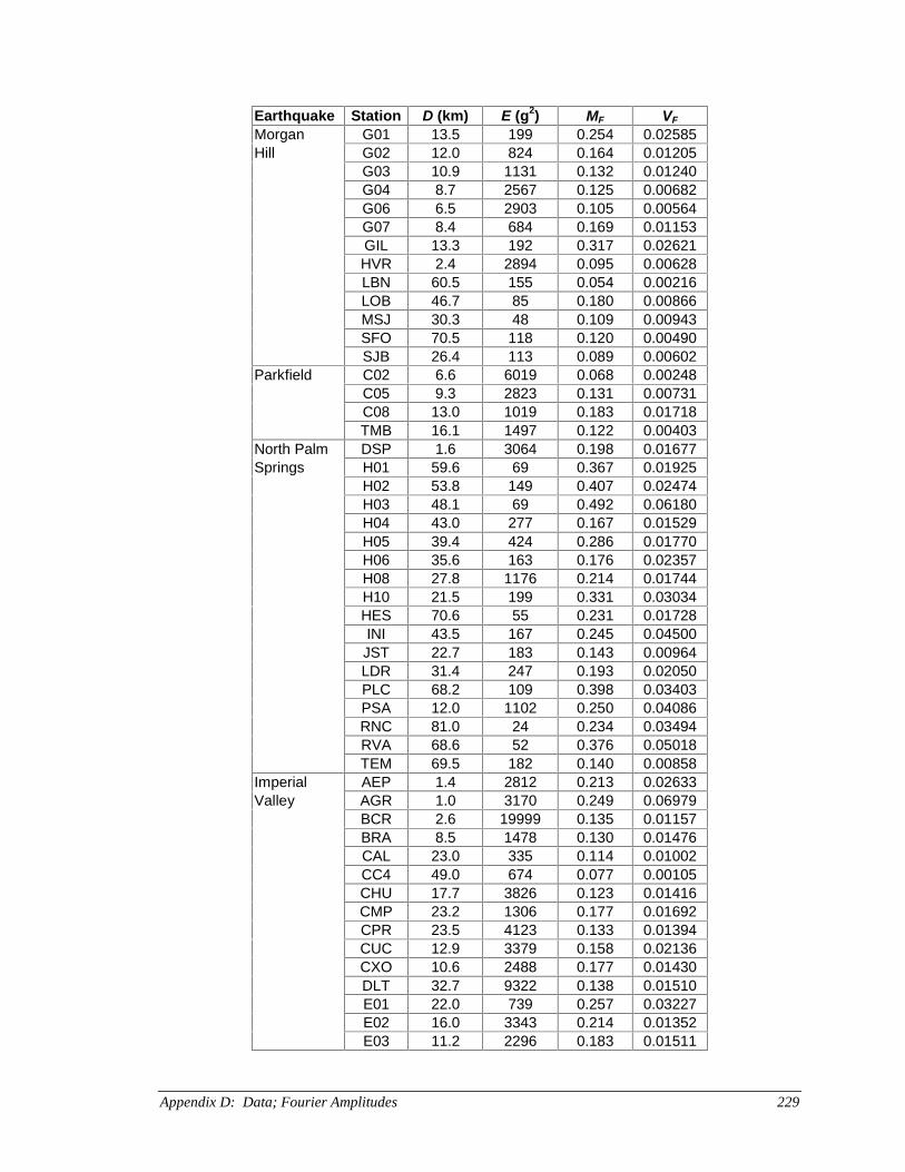
Appendix D: Data; Fourier Amplitudes 229
Earthquake Station D (km) E (g2) MF VF
Morgan G01 13.5 199 0.254 0.02585Hill G02 12.0 824 0.164 0.01205
G03 10.9 1131 0.132 0.01240G04 8.7 2567 0.125 0.00682G06 6.5 2903 0.105 0.00564G07 8.4 684 0.169 0.01153GIL 13.3 192 0.317 0.02621HVR 2.4 2894 0.095 0.00628LBN 60.5 155 0.054 0.00216LOB 46.7 85 0.180 0.00866MSJ 30.3 48 0.109 0.00943SFO 70.5 118 0.120 0.00490SJB 26.4 113 0.089 0.00602
Parkfield C02 6.6 6019 0.068 0.00248C05 9.3 2823 0.131 0.00731C08 13.0 1019 0.183 0.01718TMB 16.1 1497 0.122 0.00403
North Palm DSP 1.6 3064 0.198 0.01677Springs H01 59.6 69 0.367 0.01925
H02 53.8 149 0.407 0.02474H03 48.1 69 0.492 0.06180H04 43.0 277 0.167 0.01529H05 39.4 424 0.286 0.01770H06 35.6 163 0.176 0.02357H08 27.8 1176 0.214 0.01744H10 21.5 199 0.331 0.03034HES 70.6 55 0.231 0.01728INI 43.5 167 0.245 0.04500JST 22.7 183 0.143 0.00964LDR 31.4 247 0.193 0.02050PLC 68.2 109 0.398 0.03403PSA 12.0 1102 0.250 0.04086RNC 81.0 24 0.234 0.03494RVA 68.6 52 0.376 0.05018TEM 69.5 182 0.140 0.00858
Imperial AEP 1.4 2812 0.213 0.02633Valley AGR 1.0 3170 0.249 0.06979
BCR 2.6 19999 0.135 0.01157BRA 8.5 1478 0.130 0.01476CAL 23.0 335 0.114 0.01002CC4 49.0 674 0.077 0.00105CHU 17.7 3826 0.123 0.01416CMP 23.2 1306 0.177 0.01692CPR 23.5 4123 0.133 0.01394CUC 12.9 3379 0.158 0.02136CXO 10.6 2488 0.177 0.01430DLT 32.7 9322 0.138 0.01510E01 22.0 739 0.257 0.03227E02 16.0 3343 0.214 0.01352E03 11.2 2296 0.183 0.01511
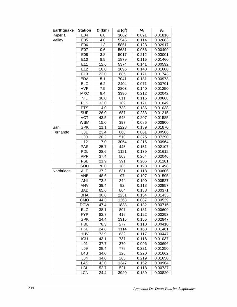
Appendix D: Data; Fourier Amplitudes230
Earthquake Station D (km) E (g2) MF VF
Imperial E04 6.8 3062 0.091 0.01816Valley E05 4.0 5545 0.114 0.02683
E06 1.3 5851 0.128 0.02917E07 0.6 5631 0.056 0.00499E08 3.8 5017 0.212 0.03001E10 8.5 1879 0.115 0.01460E11 12.6 5374 0.141 0.00592E12 18.0 1096 0.148 0.01600E13 22.0 885 0.171 0.01743EDA 5.1 7041 0.131 0.00973ELC 6.2 2404 0.071 0.00791HVP 7.5 2803 0.140 0.01250MXC 8.4 3386 0.212 0.02042NIL 36.0 611 0.116 0.00668PLS 32.0 189 0.171 0.01049PTS 14.0 738 0.136 0.01038SUP 26.0 687 0.233 0.01215VCT 43.5 648 0.207 0.01585WSM 15.0 397 0.085 0.00900
San GPK 21.1 1223 0.139 0.01870Fernando L01 23.4 860 0.081 0.00586
L09 20.2 510 0.375 0.07290L12 17.0 3054 0.216 0.00964PAS 25.7 445 0.151 0.02107PDL 28.6 1121 0.139 0.01612PPP 37.4 508 0.264 0.02046PSL 21.9 391 0.206 0.01281SOD 70.0 186 0.198 0.01498
Northridge ALF 37.2 631 0.118 0.00806ANB 48.6 97 0.197 0.01595ANI 73.2 244 0.190 0.00527ANV 39.4 92 0.118 0.00857BAD 65.6 864 0.138 0.00371BHA 30.8 2231 0.154 0.01433CMO 44.3 1263 0.087 0.00529DOW 47.4 1838 0.132 0.00715ELZ 38.1 807 0.131 0.00609FYP 82.7 416 0.122 0.00298GPK 24.4 1315 0.155 0.02847HBL 78.3 277 0.110 0.00410HSL 24.8 3114 0.163 0.01461HUV 73.9 832 0.117 0.00447IGU 43.1 737 0.118 0.01037L01 37.7 370 0.096 0.00696L09 28.4 778 0.221 0.01250L4B 34.0 126 0.220 0.01662L04 34.0 265 0.219 0.01650LAS 42.0 1347 0.152 0.00964LBL 52.7 521 0.118 0.00737LCN 24.4 3920 0.139 0.00820

Appendix D: Data; Fourier Amplitudes 231
Earthquake Station D (km) E (g2) MF VF
Northridge LNF 53.4 220 0.102 0.00744LPK 45.7 2028 0.120 0.00392LRP 48.9 744 0.148 0.00877LV1 38.6 212 0.158 0.01415LV2 38.6 210 0.164 0.01598LV3 38.7 259 0.138 0.01172LV4 38.9 299 0.108 0.01254LV5 39.2 663 0.122 0.00893LV6 39.4 1142 0.158 0.00867MCN 27.0 1070 0.366 0.05446MJO 78.0 137 0.159 0.00386MJV 86.9 90 0.119 0.00510MPK 28.3 3118 0.122 0.00422MTW 36.9 748 0.234 0.01480NBI 86.2 289 0.109 0.00411
NWH 8.4 14473 0.115 0.00434NWK 54.1 287 0.138 0.00878OBG 37.9 3708 0.196 0.00908ORR 24.6 9255 0.111 0.00511PCD 9.3 2431 0.136 0.01549PDS 35.7 789 0.137 0.00669PHN 56.0 493 0.102 0.00709PKC 9.3 5336 0.083 0.00274PMG 49.8 2291 0.106 0.00556PRD 86.8 444 0.115 0.00488PSW 34.5 1144 0.156 0.00992PVC 53.8 177 0.152 0.00702RHE 50.8 494 0.106 0.00313RNC 82.9 147 0.180 0.01810ROS 66.0 132 0.134 0.00843RVA 99.6 147 0.183 0.00348SFY 9.5 5059 0.122 0.01208SMG 27.8 9446 0.178 0.01124SNM 35.5 766 0.168 0.00988SPP 58.5 400 0.115 0.00419SSA 18.4 3611 0.275 0.03084SYH 7.6 8646 0.089 0.00543TAR 3.0 75508 0.173 0.02088TOP 23.6 3430 0.180 0.01312ULA 23.6 2896 0.235 0.03016USB 114.0 488 0.091 0.00311VLA 23.7 1565 0.097 0.00596VRP 25.3 1058 0.188 0.01638VSP 9.1 23155 0.142 0.00828
Loma A07 46.5 587 0.097 0.00748Prieta A10 46.6 854 0.057 0.00178
A2E 56.7 977 0.126 0.00973A3E 56.7 346 0.131 0.00922AGW 27.0 1304 0.100 0.00875CAP 8.6 7877 0.146 0.01705
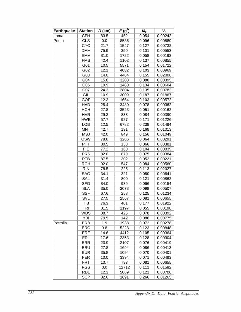
Appendix D: Data; Fourier Amplitudes232
Earthquake Station D (km) E (g2) MF VF
Loma CFH 83.5 452 0.054 0.00242Prieta CLS 0.0 8536 0.096 0.00580
CYC 21.7 1547 0.127 0.00732DMH 75.9 350 0.101 0.00553EMV 81.0 1722 0.058 0.00193FMS 42.4 1102 0.137 0.00855G01 10.5 5571 0.154 0.01722G02 12.1 4082 0.103 0.00969G03 14.0 4484 0.155 0.02008G04 15.8 3208 0.080 0.00395G06 19.9 1480 0.134 0.00604G07 24.3 2804 0.135 0.00782GIL 10.9 3009 0.187 0.01867GOF 12.3 1654 0.103 0.00572HAD 25.4 3480 0.078 0.00362HCH 27.8 3523 0.051 0.00162HVR 29.3 838 0.084 0.00390HWB 57.7 927 0.171 0.01226LOB 12.5 6782 0.238 0.01494MNT 42.7 191 0.168 0.01013MSJ 42.0 849 0.156 0.01049OSW 78.8 3286 0.064 0.00291PHT 80.5 133 0.066 0.00381PIE 77.2 160 0.104 0.00839PRS 82.0 879 0.075 0.00384PTB 87.5 302 0.052 0.00221RCH 92.0 547 0.084 0.00560RIN 78.5 225 0.113 0.02027SAG 34.1 321 0.080 0.00641SAL 31.4 800 0.121 0.00862SFG 84.0 939 0.066 0.00154SLA 35.0 3073 0.098 0.00507SSF 67.6 258 0.125 0.01234SVL 27.5 2567 0.081 0.00655TIB 76.3 401 0.177 0.01922TRI 81.5 1197 0.055 0.00198
WDS 38.7 425 0.078 0.00392YBI 79.5 142 0.086 0.00775
Petrolia ERB 1.9 1938 0.072 0.00278ERC 9.8 5228 0.123 0.00848ERF 14.6 4412 0.105 0.00364ERL 17.6 2353 0.128 0.00904ERR 23.9 2107 0.076 0.00419ERU 27.8 1694 0.086 0.00413EUR 35.8 1094 0.070 0.00401FER 10.0 3394 0.071 0.00493FRT 13.7 793 0.081 0.00655PGS 0.0 12712 0.111 0.01582RDL 12.3 5069 0.121 0.00700SCP 32.6 1691 0.266 0.01265

Appendix D: Data; Fourier Amplitudes 233
Earthquake Station D (km) E (g2) MF VF
Landers AMB 68.3 2447 0.156 0.01346BKR 88.3 854 0.129 0.00972BRN 92.4 571 0.081 0.00413BRS 37.7 731 0.098 0.01056DSP 22.5 2177 0.106 0.01087FFP 45.4 897 0.195 0.02527FTI 65.0 763 0.134 0.01178FVR 25.8 3958 0.134 0.00787H05 69.1 754 0.214 0.01883H10 51.3 223 0.246 0.03082INI 54.9 994 0.095 0.01000INO 49.6 2093 0.098 0.00506JST 11.3 7786 0.084 0.00465MVF 17.7 2303 0.084 0.00676NPS 27.7 1782 0.160 0.01487PLC 95.0 256 0.270 0.01782PSA 36.7 1181 0.143 0.02554PWS 41.9 346 0.348 0.03852RVA 95.9 204 0.249 0.02896TPP 37.7 1422 0.123 0.01585
WWT 27.6 1757 0.231 0.02033YER 26.3 2246 0.127 0.01258


Appendix E: Stations in the SMART-1 Array 235
APPENDIX ESTATIONS IN THE SMART-1 ARRAY
Table E.1: SMART-1 array station locations (Niazi, 1990).Station Longitude
(Deg East)Latitude
(Deg. North)Elevation(meters)
C-00 121.7647 24.6738 6.1I-01 121.7650 24.6755 5.9I-02 121.7660 24.6750 5.5I-03 121.7666 24.6743 6.1I-04 121.7667 24.6734 6.1I-05 121.7662 24.6725 6.3I-06 121.7652 24.6721 6.6I-07 121.7642 24.6720 6.3I-08 121.7635 24.6725 6.2I-09 121.7628 24.6732 7.0I-10 121.7628 24.6741 7.0I-11 121.7634 24.6749 6.8I-12 121.7641 24.6755 6.4M-01 121.7667 24.6825 5.0M-02 121.7717 24.6814 4.4M-03 121.7734 24.6769 4.0M-04 121.7745 24.6717 4.5M-05 121.7720 24.6682 3.9M-06 121.7677 24.6651 4.3M-07 121.7622 24.6649 5.2M-08 121.7584 24.6670 7.4M-09 121.7552 24.6704 10.8M-10 121.7557 24.6750 7.6M-11 121.7574 24.6799 7.1M-12 121.7619 24.6826 5.8O-01 121.7687 24.6917 5.3
O-02 121.7781 24.6871 4.9
O-03 121.7840 24.6791 3.4
O-04 121.7840 24.6703 2.4
O-05 121.7798 24.6622 3.8
O-06 121.7708 24.6565 4.8
O-07 121.7608 24.6560 7.2
O-08 121.7518 24.6594 18.1
O-09 121.7457 24.6675 9.6
O-10 121.7454 24.6778 13.4
O-11 121.7506 24.6857 9.1
O-12 121.7589 24.6910 6.5
E-01 121.7644 24.6487 5.2
E-02 121.7610 24.6305 9.7

Appendix F: The Northridge Earthquake Case Study; Recordings and Simulations 237
APPENDIX FTHE NORTHRIDGE EARTHQUAKE CASE STUDY;
RECORDINGS AND SIMULATIONS
The recording stations used in the 1994 Northridge, California earthquake case study that
is described in Chapter 7 are listed in this appendix. The station code is the same as in
Table A.1, where the locations of all the recording stations are tabulated. This appendix
includes four tables, each containing information on one ground motion intensity
parameter:
• Table F.1: Peak ground acceleration.
• Table F.2: Pseudo spectral acceleration corresponding to a natural period of 0.3
seconds.
• Table F.3: Pseudo spectral acceleration corresponding to a natural period of 1.0
seconds.
• Table F.4: Pseudo spectral acceleration corresponding to a natural period of 2.0
seconds.
In each table, the recorded ground motion intensity parameter is reported, along with
summary statistics from ten simulations. These summary statistics are:
• The mean.
• The standard deviation.
• The median.
• The standard deviation of the natural logarithm of the ground motion intensity
parameter; i.e., the logarithmic standard deviation.
The data that are tabulated in this appendix are presented graphically in Figures 7.2
through 7.5.

Appendix F: The Northridge Earthquake Case Study; Recordings and Simulations238
Table F.1: Recorded PGA and summary statistics from ten simulated time series.Station Recorded
PGA (g)Mean
(g)St.Dev.
(g)Median
(g)Log.St.Dev.
ALF 0.101 0.103 0.007 0.103 0.067ANB 0.068 0.041 0.006 0.041 0.151ANI 0.037 0.033 0.005 0.033 0.158BHA 0.239 0.210 0.020 0.206 0.095CMO 0.121 0.120 0.015 0.121 0.129DOW 0.177 0.189 0.028 0.182 0.149FYP 0.100 0.081 0.009 0.078 0.112HSL 0.231 0.300 0.075 0.275 0.251IGU 0.101 0.112 0.012 0.109 0.111L01 0.077 0.073 0.012 0.076 0.160L04 0.084 0.076 0.010 0.075 0.131L09 0.225 0.173 0.023 0.176 0.132LAS 0.198 0.158 0.015 0.157 0.095LBL 0.069 0.094 0.016 0.089 0.167LCN 0.256 0.301 0.026 0.301 0.086LNF 0.064 0.054 0.005 0.054 0.086LPK 0.223 0.191 0.020 0.194 0.105LV1 0.073 0.067 0.005 0.065 0.074LV2 0.063 0.066 0.008 0.065 0.118LV3 0.106 0.069 0.009 0.066 0.128LV4 0.057 0.072 0.008 0.071 0.110LV5 0.092 0.113 0.015 0.114 0.129LV6 0.178 0.182 0.023 0.189 0.127MJO 0.059 0.045 0.007 0.045 0.158MJV 0.053 0.033 0.003 0.033 0.088MPK 0.193 0.222 0.026 0.220 0.118MTW 0.133 0.137 0.014 0.135 0.106NBI 0.061 0.060 0.008 0.056 0.140NWH 0.583 0.752 0.105 0.744 0.140OBG 0.355 0.300 0.030 0.303 0.101ORR 0.568 0.597 0.096 0.602 0.161PHN 0.103 0.101 0.015 0.099 0.144PKC 0.301 0.283 0.033 0.285 0.117PMG 0.143 0.199 0.019 0.205 0.096PVC 0.054 0.052 0.005 0.053 0.095RHE 0.116 0.087 0.009 0.085 0.103RNC 0.046 0.051 0.006 0.051 0.114ROS 0.040 0.044 0.006 0.044 0.138RVA 0.064 0.051 0.010 0.047 0.189SFY 0.344 0.382 0.051 0.372 0.135SNM 0.125 0.155 0.020 0.157 0.128SPP 0.095 0.085 0.011 0.082 0.126ULA 0.278 0.297 0.024 0.297 0.082USB 0.069 0.063 0.009 0.064 0.141VRP 0.140 0.190 0.023 0.188 0.123
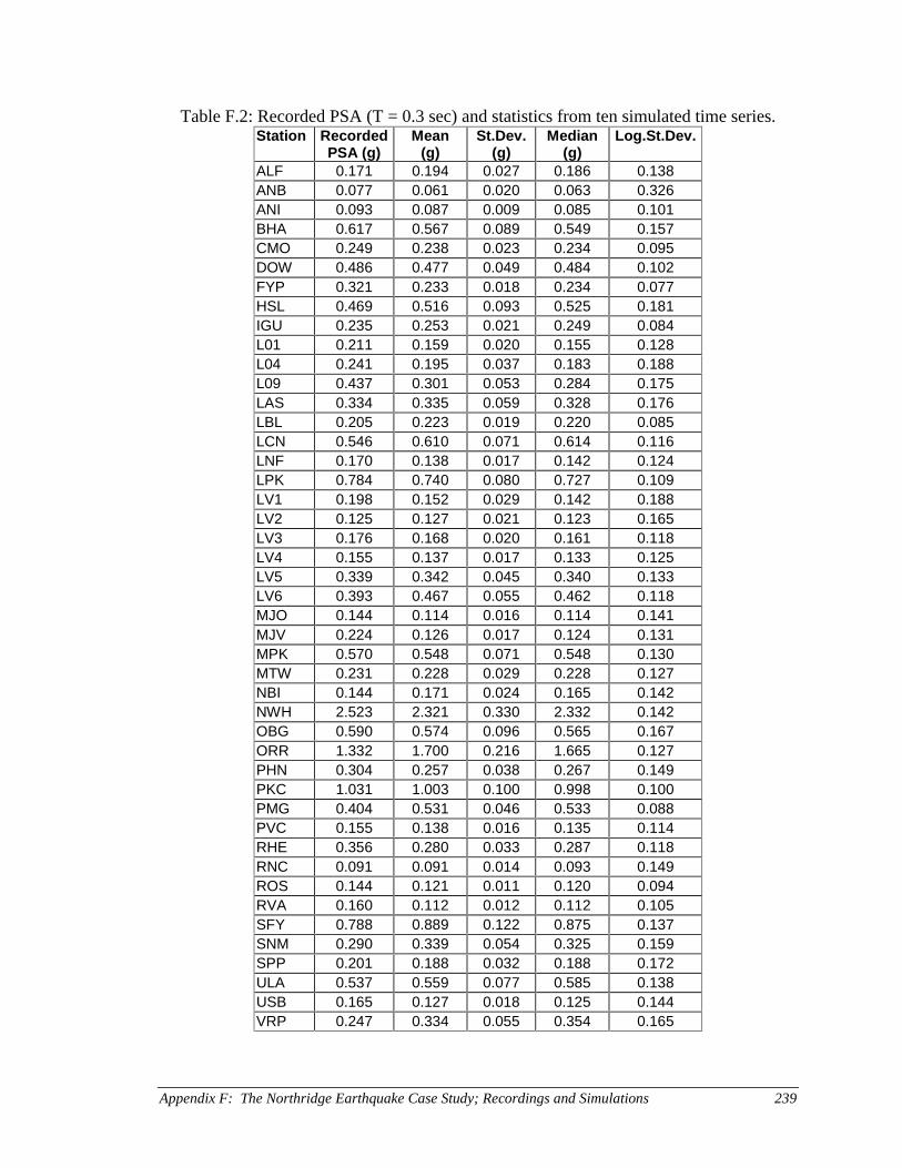
Appendix F: The Northridge Earthquake Case Study; Recordings and Simulations 239
Table F.2: Recorded PSA (T = 0.3 sec) and statistics from ten simulated time series.Station Recorded
PSA (g)Mean
(g)St.Dev.
(g)Median
(g)Log.St.Dev.
ALF 0.171 0.194 0.027 0.186 0.138ANB 0.077 0.061 0.020 0.063 0.326ANI 0.093 0.087 0.009 0.085 0.101BHA 0.617 0.567 0.089 0.549 0.157CMO 0.249 0.238 0.023 0.234 0.095DOW 0.486 0.477 0.049 0.484 0.102FYP 0.321 0.233 0.018 0.234 0.077HSL 0.469 0.516 0.093 0.525 0.181IGU 0.235 0.253 0.021 0.249 0.084L01 0.211 0.159 0.020 0.155 0.128L04 0.241 0.195 0.037 0.183 0.188L09 0.437 0.301 0.053 0.284 0.175LAS 0.334 0.335 0.059 0.328 0.176LBL 0.205 0.223 0.019 0.220 0.085LCN 0.546 0.610 0.071 0.614 0.116LNF 0.170 0.138 0.017 0.142 0.124LPK 0.784 0.740 0.080 0.727 0.109LV1 0.198 0.152 0.029 0.142 0.188LV2 0.125 0.127 0.021 0.123 0.165LV3 0.176 0.168 0.020 0.161 0.118LV4 0.155 0.137 0.017 0.133 0.125LV5 0.339 0.342 0.045 0.340 0.133LV6 0.393 0.467 0.055 0.462 0.118MJO 0.144 0.114 0.016 0.114 0.141MJV 0.224 0.126 0.017 0.124 0.131MPK 0.570 0.548 0.071 0.548 0.130MTW 0.231 0.228 0.029 0.228 0.127NBI 0.144 0.171 0.024 0.165 0.142NWH 2.523 2.321 0.330 2.332 0.142OBG 0.590 0.574 0.096 0.565 0.167ORR 1.332 1.700 0.216 1.665 0.127PHN 0.304 0.257 0.038 0.267 0.149PKC 1.031 1.003 0.100 0.998 0.100PMG 0.404 0.531 0.046 0.533 0.088PVC 0.155 0.138 0.016 0.135 0.114RHE 0.356 0.280 0.033 0.287 0.118RNC 0.091 0.091 0.014 0.093 0.149ROS 0.144 0.121 0.011 0.120 0.094RVA 0.160 0.112 0.012 0.112 0.105SFY 0.788 0.889 0.122 0.875 0.137SNM 0.290 0.339 0.054 0.325 0.159SPP 0.201 0.188 0.032 0.188 0.172ULA 0.537 0.559 0.077 0.585 0.138USB 0.165 0.127 0.018 0.125 0.144VRP 0.247 0.334 0.055 0.354 0.165
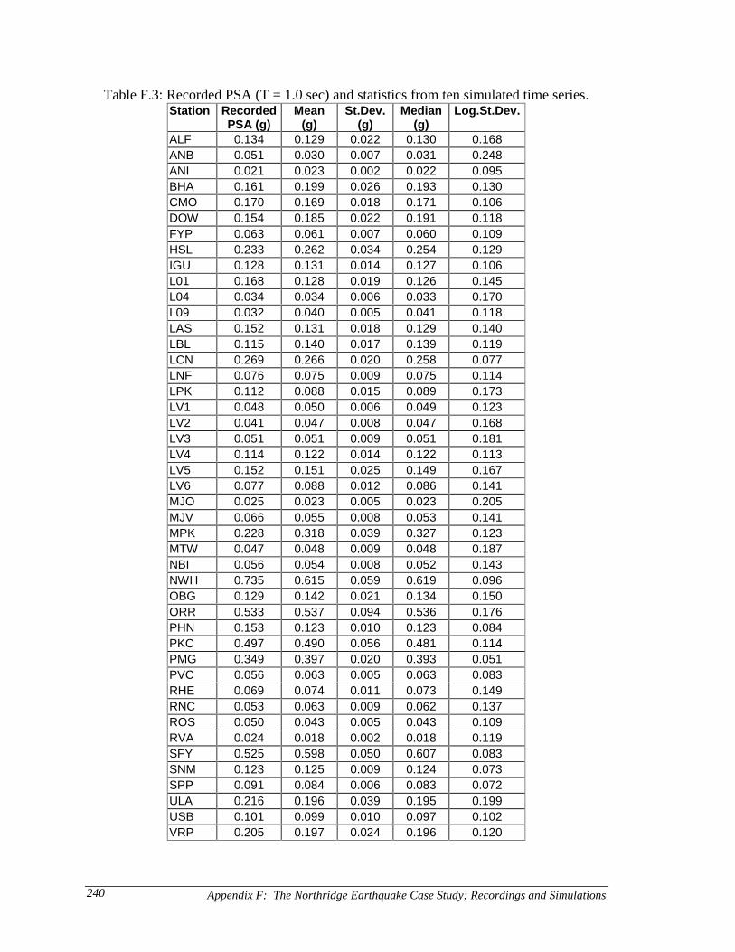
Appendix F: The Northridge Earthquake Case Study; Recordings and Simulations240
Table F.3: Recorded PSA (T = 1.0 sec) and statistics from ten simulated time series.Station Recorded
PSA (g)Mean
(g)St.Dev.
(g)Median
(g)Log.St.Dev.
ALF 0.134 0.129 0.022 0.130 0.168ANB 0.051 0.030 0.007 0.031 0.248ANI 0.021 0.023 0.002 0.022 0.095BHA 0.161 0.199 0.026 0.193 0.130CMO 0.170 0.169 0.018 0.171 0.106DOW 0.154 0.185 0.022 0.191 0.118FYP 0.063 0.061 0.007 0.060 0.109HSL 0.233 0.262 0.034 0.254 0.129IGU 0.128 0.131 0.014 0.127 0.106L01 0.168 0.128 0.019 0.126 0.145L04 0.034 0.034 0.006 0.033 0.170L09 0.032 0.040 0.005 0.041 0.118LAS 0.152 0.131 0.018 0.129 0.140LBL 0.115 0.140 0.017 0.139 0.119LCN 0.269 0.266 0.020 0.258 0.077LNF 0.076 0.075 0.009 0.075 0.114LPK 0.112 0.088 0.015 0.089 0.173LV1 0.048 0.050 0.006 0.049 0.123LV2 0.041 0.047 0.008 0.047 0.168LV3 0.051 0.051 0.009 0.051 0.181LV4 0.114 0.122 0.014 0.122 0.113LV5 0.152 0.151 0.025 0.149 0.167LV6 0.077 0.088 0.012 0.086 0.141MJO 0.025 0.023 0.005 0.023 0.205MJV 0.066 0.055 0.008 0.053 0.141MPK 0.228 0.318 0.039 0.327 0.123MTW 0.047 0.048 0.009 0.048 0.187NBI 0.056 0.054 0.008 0.052 0.143NWH 0.735 0.615 0.059 0.619 0.096OBG 0.129 0.142 0.021 0.134 0.150ORR 0.533 0.537 0.094 0.536 0.176PHN 0.153 0.123 0.010 0.123 0.084PKC 0.497 0.490 0.056 0.481 0.114PMG 0.349 0.397 0.020 0.393 0.051PVC 0.056 0.063 0.005 0.063 0.083RHE 0.069 0.074 0.011 0.073 0.149RNC 0.053 0.063 0.009 0.062 0.137ROS 0.050 0.043 0.005 0.043 0.109RVA 0.024 0.018 0.002 0.018 0.119SFY 0.525 0.598 0.050 0.607 0.083SNM 0.123 0.125 0.009 0.124 0.073SPP 0.091 0.084 0.006 0.083 0.072ULA 0.216 0.196 0.039 0.195 0.199USB 0.101 0.099 0.010 0.097 0.102VRP 0.205 0.197 0.024 0.196 0.120

Appendix F: The Northridge Earthquake Case Study; Recordings and Simulations 241
Table F.4: Recorded PSA (T = 2.0 sec) and statistics from ten simulated time series.Station Recorded
PSA (g)Mean
(g)St.Dev.
(g)Median
(g)Log.St.Dev.
ALF 0.040 0.043 0.009 0.039 0.202ANB 0.011 0.010 0.002 0.009 0.162ANI 0.007 0.007 0.001 0.007 0.105BHA 0.134 0.140 0.015 0.137 0.105CMO 0.066 0.061 0.007 0.060 0.113DOW 0.068 0.080 0.010 0.082 0.121FYP 0.008 0.009 0.002 0.009 0.179HSL 0.094 0.104 0.015 0.101 0.145IGU 0.050 0.071 0.011 0.068 0.153L01 0.029 0.031 0.003 0.031 0.085L04 0.015 0.021 0.002 0.020 0.094L09 0.024 0.030 0.004 0.030 0.138LAS 0.057 0.062 0.006 0.062 0.104LBL 0.049 0.058 0.006 0.059 0.108LCN 0.141 0.158 0.019 0.154 0.119LNF 0.039 0.050 0.005 0.050 0.094LPK 0.032 0.020 0.003 0.020 0.136LV1 0.051 0.055 0.003 0.054 0.050LV2 0.060 0.065 0.004 0.063 0.068LV3 0.059 0.064 0.004 0.065 0.059LV4 0.095 0.097 0.006 0.099 0.066LV5 0.113 0.107 0.009 0.108 0.088LV6 0.064 0.067 0.005 0.067 0.073MJO 0.008 0.008 0.001 0.007 0.173MJV 0.007 0.009 0.001 0.009 0.089MPK 0.084 0.095 0.013 0.099 0.142MTW 0.012 0.018 0.002 0.017 0.134NBI 0.038 0.045 0.004 0.045 0.087NWH 0.260 0.333 0.033 0.341 0.099OBG 0.051 0.068 0.007 0.068 0.104ORR 0.226 0.255 0.020 0.251 0.079PHN 0.055 0.066 0.006 0.066 0.095PKC 0.110 0.123 0.018 0.121 0.146PMG 0.074 0.089 0.010 0.089 0.109PVC 0.012 0.013 0.002 0.013 0.121RHE 0.014 0.019 0.002 0.018 0.135RNC 0.024 0.020 0.003 0.019 0.142ROS 0.014 0.012 0.001 0.012 0.119RVA 0.010 0.010 0.001 0.010 0.109SFY 0.167 0.188 0.021 0.192 0.111SNM 0.023 0.025 0.004 0.025 0.150SPP 0.016 0.016 0.001 0.016 0.072ULA 0.058 0.096 0.009 0.098 0.099USB 0.031 0.037 0.005 0.038 0.143VRP 0.051 0.044 0.006 0.042 0.127


References 243
REFERENCES
Abrahamson, N.A. (1985). “Estimation of seismic wave coherency and rupture velocityusing the SMART 1 strong-motion array recordings.” EERC Report No.UCB/EERC-85/02. Earthquake Engineering Research Center, University ofCalifornia, Berkeley, CA, USA.
Abrahamson, N.A., and J.P. Singh (1986). “Importance of phasing of strong groundmotion in the estimation of structural response.” Proceedings of the 3rd
Conference on Dynamic Response of Structures, 86-93.
Abrahamson, N.A., and B.A. Bolt (1987). “Array analysis and synthesis mapping ofstrong seismic motion.” in Strong Motion Synthesis (B.A. Bolt, ed.). AcademicPress, Orlando.
Abrahamson, N.A., B.A. Bolt, R.B. Darragh, J. Penzien, and Y.B. Tsai (1987). “TheSMART-1 accelerograph array (1980-1987): a review.” Earthquake Spectra 3,263-287.
Abrahamson, N.A., J.F. Schneider, and J.C. Stepp (1991). “Empirical spatial coherencyfunctions for application to soil-structure interaction analyses.” EarthquakeSpectra 7, 1-27.
Aki, K. (1968). “Seismic displacements near a fault.” J. Geophys. Res. 73, 5359-5376.
Aki, K., and P.G. Richards (1980). Quantitative Seismology, Theory and Methods, Vol. Iand II. Freeman, San Francisco, CA, USA.
Anderson, J.G., and S.E. Hough (1984). “A model for the shape of the Fourier amplitudespectrum of acceleration at high frequencies.” Bull. Seism. Soc. Am. 74, 1069-1993.
Archuleta, R.J., and S.M. Day (1980). “Dynamic rupture in a layered medium: the 1966Parkfield earthquake.” Bull. Seism. Soc. Am. 70, 671-689.
Arias, A. (1970). “A measure of earthquake intensity.” in Seismic Design of NuclearPower Plants (edited by R. Hansen), MIT Press, Cambridge, MA, USA, 438-483.
Atkinson, G.M. (1996). “The high-frequency shape of the source spectrum forearthquakes in Eastern and Western Canada.” Bull. Seism. Soc. Am. 86, 106-112.
Atkinson, G.M., and D.M. Boore (1995). “Ground-motion relations for eastern NorthAmerica.” Bull. Seism. Soc. Am. 85, 17-30.
Bolt, B.A., C.H. Loh, J. Penzien, Y.B. Tsai, and Y.T. Yeh (1982). “Preliminary report onthe SMART 1 strong motion array in Taiwan.” EERC Report No. UCB/EERC-82/13. Earthquake Engineering Research Center, University of California,Berkeley, CA, USA.
Bolt, B.A., R.A. Uhrhammer, and R.B. Darragh (1985). “The Morgan Hill earthquake ofApril 24, 1984 – seismological aspects.” Earthquake Spectra 1, 407-418.

References244
Boore, D.M. (1983). “Stochastic simulation of high-frequency ground motions based onseismological models of the radiated spectra.” Bull. Seism. Soc. Am. 73, 1865-1894.
Boore, D.M. (1986). “Short-period P- and S-wave radiation from large earthquakes:implications for spectral scaling relations.” Bull. Seism. Soc. Am. 76, 43-64.
Boore, D.M., W.B. Joyner, and T.E. Fumal (1993). “Estimation of response spectra andpeak accelerations from western North American earthquakes: an interim report.”U.S. Geol. Survey Open-File Report 93-509.
Boore, D.M., W.B. Joyner, and T.E. Fumal (1994). “Estimation of response spectra andpeak accelerations from western North American earthquakes: an interim report,part 2.” U.S. Geol. Survey Open-File Report 94-127.
Boore, D.M., W.B. Joyner, and T.E. Fumal (1997). “Equations for estimating horizontalresponse spectra and peak acceleration from western North Americanearthquakes: a summary of recent work.” Seism. Res. Lett. 68, 128-153.
Borcherdt, R.D. (1994). “Estimates of site-dependent response spectra for design(methodology and justification).” Earthquake Spectra 10, 617-653.
Bouchon, M. (1982). “The rupture mechanism of the Coyote Lake earthquake of 6August 1979 inferred from near-field data.” Bull. Seism. Soc. Am. 72, 745-757.
Brune, J.N. (1970). “Tectonic stress and the spectra of seismic shear waves fromearthquakes.” J. Geophys. Res. 75, 4997-5009.
Brune, J.N. (1971). “Correction.” J. Geophys. Res. 76, 5002.
BSSC (1994). NEHRP Recommended Provisions for Seismic Regulations for NewBuildings. Part I – Provisions. FEMA 222A, Federal Emergency ManagementAgency.
Campbell, K.W. (1987). “Predicting strong ground motion in Utah.” in Assessment ofRegional Earthquake Hazards and Risks Along the Wasatch Front, Utah II (editedby P.L. Gori and W.W. Hays). U.S. Geol. Survey Open-File Report 87-585, L1-L90.
Chang, S.W., J.D. Bray, and R.B. Seed (1996). “Engineering implications of groundmotions from the Northridge earthquake.” Bull. Seism. Soc. Am. 86, S270-S288.
Chavez, D., J. Gonzales, A. Reyes, J.N. Brune, F.L. Vernon, R. Simons, L.K. Hutton,P.T. German, and C.E. Johnson (1982). “Main-shock location and magnitudedetermination using combined U.S. and Mexican data.” in The Imperial ValleyEarthquake of October 15, 1979. U.S. Geol. Survey Professional Paper 1254, 51-54.
Clough, R.W., and J. Penzien (1975). Dynamics of Structures. McGraw-Hill, New York,NY, USA.
Conte, J.P., K.S. Pister, and S.A. Mahin (1992). “Nonstationary ARMA modeling ofseismic motions.” J. Soil Dyn. and Earthquake Eng. 11, 411-426.

References 245
Converse, A.M., and A.G. Brady (1992). “BAP: Basic strong-motion accelerogramprocessing software, version 1.0.” U.S. Geol. Survey Open-File Report 92-296A.
Der Kiureghian, A. (1996). “A coherency model for spatially varying ground motions.”Earthquake Eng. Struct. Dyn. 25, 99-111.
Ellis, G.W., A.S. Cakmak, and J. Ledolter (1987). “Modelling earthquake groundmotions in seismically active regions using parametric time series methods.” inGround Motion and Engineering Seismology (edited by A.S. Cakmak), Elsevier,Amsterdam, Holland, 551-566.
Hagerty, M.T., and S.Y. Schwartz (1996). “The Cape Mendocino earthquake: broadbanddetermination of source parameters.” J. Geophys. Res. 101, 16043-16058.
Hanks, T.C. (1982). “fmax.” Bull. Seism. Soc. Am. 72, 1867-1879.
Hanks, T.C., and H. Kanamori (1979). “A moment magnitude scale.” J. Geophys. Res.84, 2348-2350.
Hao, H. (1989). “Effects of spatial variation of ground motion on large multiply-supported structures.” Report No. UCB/EERC-89/06, Earthquake EngineeringResearch Center, University of California, Berkeley, CA, USA.
Harichandran, R.S., and E.H. Vanmarcke (1984). “Space-time variation of earthquakeground motion.” Research Report R84-12, Dept. of Civil Engineering, MIT,Cambridge, MA, USA.
Harichandran, R.S., and E.H. Vanmarcke (1986). “Stochastic variation of earthquakeground motion in space and time.” J. Eng. Mech. 112, 154-174.
Hartzell, S.H. (1978). “Earthquake aftershocks as Green’s functions.” Geophys. Res. Lett.5, 1-4.
Haskell, N.A. (1969). “Elastic displacements in the near-field of a propagating fault.”Bull. Seism. Soc. Am. 59, 865-908.
Hauksson, E., L.M. Jones, K. Hutton, and D. Eberhart-Phillips (1993). “The 1992Landers earthquake sequence: seismological observations.” J. Geophys. Res. 98,19835-19858.
Hauksson, E., and L.M. Jones (1995). “Seismology.” in Northridge Earthquake ofJanuary 17, 1994 Reconnaissance Report, Volume 1 (edited by J.F. Hall),supplement C to Volume 11 of Earthquake Spectra. Earthquake EngineeringResearch Institute Publication 95-03, EERI, Oakland, CA, USA, 1-12.
Jones, L.M, and E. Hauksson (1988). “The Whittier Narrows, California earthquake ofOctober 1, 1987 – seismology.” Earthquake Spectra 4, 43-53.
Joyner, W.B., and D.M. Boore (1981). “Peak horizontal acceleration and velocity fromstrong-motion records including records from the 1979 Imperial Valley,California, earthquake.” Bull. Seism. Soc. Am. 71, 2011-2038.
Joyner, W.B., and D.M. Boore (1988). “Measurement, characterization, and prediction ofstrong ground motion.” in Earthquake Engineering and Soil Dynamics II – Recent
References246
Advances in Ground-Motion Evaluation (edited by J.L. Von Thun), ASCEGeotechn. Spec. Publ. No. 20, 43-102.
Kanai, K. (1957). “Semi-empirical formula for the seismic characteristics of the ground.”Univ. Tokyo Bull. Earthquake Res. Inst. 35, 309-325.
Kanamori, H., and J. Regan (1982). “Long-period surface waves.” in The Imperial ValleyEarthquake of October 15, 1979. U.S. Geol. Survey Professional Paper 1254, 55-58.
Kanda, J., R. Iwasaki, Y. Ohsaki, T. Masao, Y. Kitada, and K. Sakata (1983).“Generation of simulated earthquake ground motions considering target responsespectra of various damping ratios.” Transactions of the 7th InternationalConference on Structural Mechanics in Reactor Technology, Vol. K(a), 71-79.
Kasahara, K. (1981). Earthquake Mechanics. Cambridge University Press, Cambridge,England, UK.
Kozin, F. (1988). “Autoregressive moving average models of earthquake records.” Prob.Eng. Mech. 3, 58-63.
Kubo, T. (1987). “The importance of phase properties in generation of syntheticearthquake strong motions.” Transactions of the 9th International Conference onStructural Mechanics in Reactor Technology, Vol. K1, 49-54.
Lindgren, B.W. (1976). Statistical Theory (3rd edition). Macmillan Publishing Co., NewYork, NY, USA.
Loh, C.H. (1985). “Analysis of the spatial variation of seismic waves and groundmovements from the SMART-1 array data.” Earthquake Eng. Struct. Dyn. 13,561-581.
Madsen, H.O., S. Krenk, and N.C. Lind (1986). Methods of Structural Safety. Prentice-Hall, Englewoods Cliffs, NJ, USA.
Marven, C., and G. Ewers (1996). A Simple Approach to Digital Signal Processing. JohnWiley & Sons, New York, NY, USA.
Matsukawa, K., M. Watabe, N.A. Theofanopulos, and M. Tohdo (1987). “Phasecharacteristics of earthquake ground motions and those applications to syntheticones.” Transactions of the 9th International Conference on Structural Mechanicsin Reactor Technology, Vol. K1, 43-48.
McGuire, R.K., A.M. Becker, and N.C. Donovan (1984). “Spectral estimates of seismicshear waves.” Bull. Seism. Soc. Am. 74, 1427-1440.
Moehle, J., G. Fenves, R. Mayes, N. Priestley, F. Seible, C.M. Uang, S. Werner, and M.Ascheim (1985). “Highway bridges and traffic management.” in NorthridgeEarthquake of January 17, 1994 Reconnaissance Report, Volume 1 (edited byJohn F. Hall), supplement C to Volume 11 of Earthquake Spectra. EarthquakeEngineering Research Institute Publication 95-03, EERI, Oakland, CA, USA,287-372.

References 247
Naraoka, K., and T. Watanabe (1987). “Generation of nonstationary earthquake groundmotions using phase characteristics.” Transactions of the 9th InternationalConference on Structural Mechanics in Reactor Technology, Vol. K1, 37-42.
Nelder, J.A., and R. Mead (1964). “A simplex method for function minimization.” TheComputer Journal 7, 308-313.
Newland, D.E. (1993). An Introduction to Random Vibrations, Spectral and WaveletAnalysis, 3rd edition. Longman, Essex, England, UK.
Niazi, M. (1990). “Behavior of peak values and spectral ordinates of near-source strongground motion over the SMART 1 array.” EERC Report No. UCB/EERC-90/17.Earthquake Engineering Research Center, University of California, Berkeley, CA,USA.
Nigam, N.C. (1982). “Phase properties of a class of random processes.” Earthquake Eng.Struct. Dyn. 10, 711-717.
NOAA (1996). Earthquake Strong Motion CD-ROM Collection. National Oceanic andAtmospheric Administration, National Environmental Satellite, Data, andInformation Service, National Geophysical Data Center, Boulder, CO, USA.
Ohsaki, Y. (1979). “On the significance of phase content in earthquake ground motions.”Earthquake Eng. Struct. Dyn. 7, 427-439.
Oliviera, C.S. (1985). “Variability of strong ground motion characteristics obtained inSMART-1 array.” Proceedings of the 12th Regional Seminar on EarthquakeEngineering, Halkidiki, Greece.
Pacheco, J., and J. Nabelek (1988). “Source mechanisms of three moderate Californiaearthquakes of July 1986.” Bull. Seism. Soc. Am. 78, 1907-1929.
Papageorgiou, A.S., and K. Aki (1983). “A specific barrier model for the quantitativedescription of inhomogeneous faulting and the prediction of strong groundmotion. Part I. Description of the model.” Bull. Seism. Soc. Am. 73, 693-722.
Park, S., and S. Elrick (1998). “Predictions of shear-wave velocities in southernCalifornia using surface geology.” Bull. Seism. Soc. Am. 88, 677-685.
Priestley, M.B. (1967). “Power spectral analysis of non-stationary processes.” J. Soundand Vibration 6, 86-97.
Reiter, L. (1990). Earthquake Hazard Analysis – Issues and Insight. Columbia UniversityPress, New York, NY, USA.
Rice, S.O. (1944). “Mathematical analysis of random noise.” Bell Syst. Techn. J. 23, 282-332.
Sabetta, F., and A. Pugliese (1996). “Estimation of response spectra and simulation ofnonstationary earthquake ground motions.” Bull. Seism. Soc. Am. 86, 337-352.
Sadigh, K., C.Y. Chang, J.A. Egan, F. Makdisi, and R.R. Youngs (1997). “Attenuationrelationships for shallow crustal earthquakes based on California strong motiondata.” Seism. Res. Lett. 68, 180-189.

References248
Seed, H.B., C. Ugas, and J. Lysmer (1976). “Site-dependent spectra for earthquake-resistant design.” Bull. Seism. Soc. Am. 66, 221-243.
Shinozuka, M., and G. Deodatis (1988). “Stochastic process models for earthquakeground motion.” Prob. Eng. Mech. 3, 114-123.
Sigbjörnsson, R., G.I. Baldvinsson, H. Thráinsson, S. Ólafsson, G.Th. Gardarsdóttir, andÓ Thórarinsson (1994). “On seismic hazard in Iceland – a stochastic simulationapproach.” Proceedings of the 10th European Conference on EarthquakeEngineering, A.A. Balkema, Rotterdam, 111-116.
Somerville, P.G. (1997). “Engineering characteristics of near fault ground motion.”Proceedings of the SMIP97 Seminar on Utilization of Strong-Motion Data, 9-28.
Somerville, P.G., N.F. Smith, R.W. Graves, and N.A. Abrahamson (1997). “Modificationof empirical strong ground motion attenuation relations to include the amplitudeand duration effect of rupture directivity.” Seism. Res. Lett. 68, 199-222.
Spudich, P., and S.H. Hartzell (1985). “Predicting earthquake ground-motion time-histories.” in Evaluating Earthquake Hazards in the Los Angeles Region – AnEarth-Science Perspective (edited by J.I. Ziony). U.S. Geol. Survey ProfessionalPaper 1360, 249-261.
Suzuki, S., and A.S. Kiremidjian (1988). “A stochastic ground motion forecast modelwith geophysical considerations.” The John A. Blume Earthquake EngineeringCenter Report No. 88, Stanford University, Stanford, CA, USA.
Sveshnikov, A.A. (1968). Problems in Probability Theory, Mathematical Statistics andTheory of Random Functions, translated from Russian by Richard A. Silverman.Dover, New York, NY, USA.
Tajimi, H. (1960). “A statistical method of determining the maximum response of abuilding structure during an earthquake.” Proc. 2nd World Conf. Earthquake Eng.,Vol. II, 781-798.
Tinsley, J.C., and T.E. Fumal (1985). “Mapping Quaternary sedimentary deposits foraerial variations in shaking response.” in Evaluating Earthquake Hazards in theLos Angeles Region – An Earth-Science Perspective (edited by J.I. Ziony). U.S.Geol. Survey Professional Paper 1360, 101-126.
Wald, D.J., D.V. Helmberger, and T.H. Heaton (1991). “Rupture model of the 1989Loma Prieta earthquake from the inversion of strong-motion and broadbandteleseismic data.” Bull. Seism. Soc. Am. 81, 1540-1572.
Wald, D.J., and T.H. Heaton (1994). “A dislocation model of the 1994 Northridge,California earthquake determined from strong ground motions.” U.S. Geol.Survey Open-File Report 94-278.
Westermo, B. (1992). “The synthesis of strong ground motion accelerograms fromexisting records.” Earthquake Eng. Struct. Dyn. 21, 743-756.
Whitcomb, J.H., C.R. Allen, J.D. Garmany, and J.A. Hileman (1973). “San Fernandoearthquake series, 1971; focal mechanisms and tectonics.” Rev. of Geophys. andSpace Phys. 11, 693-730.

References 249
Winterstein, S. (1991). “Nonlinear effects on ship bending in random seas.” TechnicalReport No. 91-2032, Det Norske Veritas, Høvik, Norway.
Zembaty, Z., and S. Krenk (1993). “Spatial seismic excitations and response spectra.” J.Eng. Mech. 119, 2449-2460.


