
Denoising and Artefact Reduction in Dynamic Flat
Detector CT Perfusion Imaging using High Speed
Acquisition: First Experimental and Clinical Results
Michael T. Manhart1,2, André Aichert1,2, Tobias Stru�ert2, Yu
Deuerling-Zheng3, Markus Kowarschik3, Andreas K. Maier1,
Joachim Hornegger1,4, and Arnd Doer�er2
1Pattern Recognition Lab, Department of Computer Science,
Friedrich-Alexander-Universität Erlangen-Nürnberg, Martensstr. 3, 91058 Erlangen,
Germany2Department of Neuroradiology, Universitätsklinikum Erlangen, Schwabachanlage 6,
91054 Erlangen, Germany3Siemens AG, Angiography & Interventional X-Ray Systems, Siemensstraÿe 1, 91301
Forchheim, Germany4Erlangen Graduate School in Advanced Optical Technologies (SAOT),
Paul-Gordan-Str. 6, 91052 Erlangen, Germany
E-mail: [email protected]
Abstract. Flat detector CT perfusion (FD-CTP) is a novel technique using C-arm
angiography systems for interventional dynamic tissue perfusion measurement with
high potential bene�ts for catheter-guided treatment of stroke. However, FD-CTP is
challenging since C-arms rotate slower than conventional CT systems. Furthermore,
noise and artefacts a�ect the measurement of contrast agent �ow in tissue. Recent
robotic C-arms are able to use high speed protocols (HSP), which allow sampling of
the contrast agent �ow with improved temporal resolution. However, low angular
sampling of projection images leads to streak artefacts, which are translated to the
perfusion maps. We recently introduced the FDK-JBF denoising technique based on
Feldkamp (FDK) reconstruction followed by joint bilateral �ltering (JBF). As this edge-
preserving noise reduction preserves streak artefacts, an empirical streak reduction
(SR) technique is presented in this work. The SR method exploits spatial and temporal
information in the form of total variation and time-curve analysis to detect and remove
streaks. The novel approach is evaluated in a numerical brain phantom and a patient
study. An improved noise and artefact reduction compared to existing post-processing
methods and faster computation speed compared an algebraic reconstruction method
are achieved.
Keywords : Flat Detector CT, 3D Reconstruction, Perfusion Imaging, Stroke Treatment,
Noise Reduction

Denoising and Artefact Reduction in Dynamic Flat Detector CT Perfusion Imaging 2
1. Introduction
Imaging of brain perfusion is a routine method in the emergency work-up of patients
suspected to su�er from acute ischemic stroke (AIS). Commonly, CT perfusion (CTP)
is used to identify stroke-a�ected tissue by acquiring hemodynamic information on the
capillary level of the brain (Miles & Gri�ths 2003). Time-concentration curves (TCCs)
in tissue and vessels are extracted from a time series of CT brain volumes acquired after
a contrast bolus injection. The hemodynamics are visualized by perfusion parameter
maps, representing quantities such as cerebral blood �ow (CBF), cerebral blood volume
(CBV), mean transit time (MTT), and time-to-peak (TTP). The parameter maps
provide important information about the extent of the stroke and allow for the
identi�cation of potentially salvageable ischemic tissue (penumbra). If the stroke is
diagnosed in a time window of up to 4.5 hours after onset, a common treatment is intra-
venous (IV) thrombolytic therapy (Hacke et al. 2008). A meta analysis of stroke therapy
articles (Rha & Saver 2007) showed a strong relation of successful vessel recanalization
to the �nal clinical outcome in AIS. The meta analysis reported that the recanalization
rate with IV thrombolytic therapy was approximately twice the spontaneous rate, but
still less than half of all cases. Techniques to improve this modest recanalization rate
are desirable.
In recent years, interventional intra-arterial (IA) stroke therapy procedures were
introduced to improve the recanalization rate and the treatment outcome. Interventional
treatment procedures of AIS are IA thrombolytic therapy (Furlan et al. 1999) and
recanalization of occluded arteries using mechanical endovascular retrieval devices
(Zaidat et al. 2008). For interventional stroke management, the patient needs to be
transported to an interventional suite equipped with a C-arm angiography system.
Recent generations of C-arm systems provide an option to reconstruct CT like volumes,
e.g., to detect haemorrhages (Stru�ert et al. 2009). However, due to hardware
limitations, dynamic interventional perfusion imaging is challenging and not yet
clinically available. If �at detector CT could provide equal information as conventional
CT regarding the brain parenchyma, the vessel status, and perfusion, then patients
could be directly referred to the interventional suite, saving the time of moving the
patient from a CT scanner room. Furthermore, dynamic perfusion imaging with �at
detector CT (FD-CTP) would allow intraoperative monitoring of the brain perfusion.
Ahmed et al. (Ahmed et al. 2009) proposed a method using a steady state contrast
injection protocol to acquire CBV maps with �at detector CT. Clinical patient studies
showed a high correlation of the C-arm CBV maps to CBV maps acquired with CTP
(Stru�ert et al. 2010, Stru�ert et al. 2011, Stru�ert et al. 2012). However, CBV maps
are limited to depict the infarct core but not the full extent of ischemic tissue. Therefore,
the development of time-resolved perfusion �at detector imaging is desirable.
FD-CTP is challenging, since common C-arm systems are not able to rotate
continuously by more than 360° and typically need ∼ 5 s to acquire one volume. This
limits the temporal resolution of the acquired TCCs. Furthermore, perfusion imaging

Denoising and Artefact Reduction in Dynamic Flat Detector CT Perfusion Imaging 3
is highly sensitive to noise, since the peaks of the TCCs inside the brain tissue typically
lie in a range of 5�30 HU. Recently, novel techniques to overcome these challenges were
proposed. Fieselmann et al. (Fieselmann et al. 2012) introduced a scanning protocol
combining interleaved scanning and partial reconstruction interpolation for improved
temporal sampling of TCCs. However, this approach requires multiple scanning
sequences, which increases radiation and contrast agent dose to the patient and limits its
clinical applicability. Wagner et al. (Wagner et al. 2013), Neukirchen et al. (Neukirchen
et al. 2010) and Manhart et al. (Manhart, Kowarschik, Fieselmann, Deuerling-
Zheng, Royalty, Maier & Hornegger 2013) presented dynamic algebraic reconstruction
algorithms to reconstruct TCCs with increased temporal resolution from the acquired
X-ray projection data by modelling the TCCs using gamma-variate functions (Wagner
et al.) as well as Gaussian (Neukirchen et al.) and spline (Manhart et al.) basis
functions. The algebraic approaches have a high computational e�ort and are sensitive
to patient motion, because they rely on subtraction of mask projection data with static
anatomical structures, e.g., skull and brain tissue, from the projection data with contrast
agent enhancement. If the patient head moves during the projection data acquisition,
the compensation of the 3D head movement on the 2D projection data is particularly
di�cult. These limitations may impede their application in clinical practice.
A novel possibility to acquire TCCs with improved temporal resolution are robotic
C-arm systems (Artis zeego, Siemens AG, Germany). The Artis zeego system provides
a high speed protocol (HSP) with increased C-arm rotation speed of up to 100°/s,
thus allowing for the acquisition of projection data for one brain volume in less than
3 s. Royalty et al. (Royalty et al. 2013) evaluated the HSP in an experimental study
measuring the brain perfusion of canines with induced focal ischemic regions. A strong
correlation of FD-CTP maps to CTP maps as gold standard was reported. However,
the results showed only a fair intra-observer performance in ischemic lesion mismatch
detection and a consistent overestimation of CBF and CBV values in FD-CTP. Recently,
Manhart et al. (Manhart, Fieselmann, Deuerling-Zheng & Kowarschik 2013) proposed
the FDK-JBF reconstruction scheme based on Feldkamp (FDK) (Feldkamp et al. 1984)
reconstruction followed by iterative denoising in volume space using joint bilateral
�ltering (JBF) (Petschnigg et al. 2004). The evaluation based on a digital brain phantom
(Riordan et al. 2011) study showed the potential of the FDK-JBF approach to improve
the noise reduction in brain tissue and to reduce the CBV and CBF overestimation.
Furthermore, the FDK-JBF technique produced brain perfusion maps with a quality
comparable to computationally more expensive algebraic reconstruction techniques, e.g.,
based on total variation (TV) minimization (Ritschl et al. 2011). However, motion of
the patient's head was not considered in this study. It is likely that the patient moves
during the acquisition procedure, especially because there is a pause of ∼ 10 s between
the acquisition of the mask projection images and the bolus projection images (with
contrast agent enhancement). During the pause the contrast medium is injected intra-
venously and transported to the intracranial arteries. In a recent publication (Manhart,
Aichert, Kowarschik, Deuerling-Zheng, Stru�ert, Doer�er, Maier & Hornegger 2013),

Denoising and Artefact Reduction in Dynamic Flat Detector CT Perfusion Imaging 4
0 5 10 15 20 25 30 35 400
50
100
150
200
Time after acquisition start [s]
C−
arm
ang
le [°]
Tr
Tw
Figure 1: C-arm position during bolus volume acquisitions using the high speed FD-CTP
protocol.
we discussed that this motion can cause severe artefacts in the perfusion maps. Due to
limitations in the detector read-out rate, the angular sampling of the projection data
in high speed scanning is coarse. This leads to streak artefacts in the reconstructed
volumes. Mask volumes with static anatomical structures are subtracted from the
volumes with contrast agent enhancement to compute volumes with pure contrast agent
enhancement (bolus volumes). The streaks vanish in the bolus volumes since they
are mainly caused by the patient's skull and are similar in the mask volumes and the
volumes with contrast agent enhancement. If patient motion occurs between the C-arm
rotations, it can be compensated by rigid registration. However, the streaks will not
cancel out during subtraction in case of even slight errors in registration due to their
high frequency structure. In (Manhart, Aichert, Kowarschik, Deuerling-Zheng, Stru�ert,
Doer�er, Maier & Hornegger 2013), we described the FDK-SR-JBF technique, which
extends the FDK-JBF approach by a streak removal (SR) for FD-CTP data. This work
discusses our streak and noise reduction algorithm in more detail, includes alternative
techniques in the evaluation (e.g., the TIPS �lter (Mendrik et al. 2011)), and shows an
additional patient study case with pre- and post-treatment acquisition.
This article is organized as follows. First, the acquisition process and protocols are
detailed. Second, the novel reconstruction and �ltering algorithm is described in detail
and an overview of the alternative approaches used in the evaluation is provided. Finally,
the FDK-SR-JBF approach is evaluated in comparison to the alternative methods with
numerical brain phantom data and clinical patient data.
2. Methods
2.1. High Speed Acquisition Protocol
Unlike traditional CT gantries, current C-arm systems cannot rotate continuously
around the patient multiple times. In order to perform time-resolved imaging, it is
therefore necessary to rotate in a bi-directional manner, following a forward-backward

Denoising and Artefact Reduction in Dynamic Flat Detector CT Perfusion Imaging 5
view-angle increment 1.5°
number of views per rotation 248
angular range per rotation 198°
time per rotation (Tr) 2.6/2.8 s
time between rotations (Tw) 1/1.2 s
number of rotations (Nrot) 7/10
source-to-detector distance 1200 mm
detector pixel size 0.616× 0.616 mm2
number of detector pixels 616× 480
after 4× 4 re-binning
total detector size ≈ 380× 296 mm2
tube peak voltage 82 kVp
system dose 1.2 µGy / projection
Table 1: Parameters of C-arm acquisition system.
pattern. The C-arm rotates multiple times in alternating directions and is forced to stop
for a short period of time before it can turn around. Recent robotic C-arm systems are
capable of performing a high speed protocol (HSP) (Artis zeego, Siemens AG, Germany).
Each rotation of the HSP scan acquires 133 projections over a 198° angular range and
requires Tr = 2.6 − 2.8 s for data acquisition with a pause of Tw = 1 − 1.2 s between
any two successive rotations. Thus, TCCs can be acquired with a temporal sampling
distance of Ts = Tr + Tw = 3.6 − 4 s. First, mask projection images are acquired in
a forward and a backward C-arm rotation before bolus injection. Mask projections in
both directions are acquired because the positions of X-ray source and detector are not
exactly the same for the forward and backward rotations. Subsequently, the contrast
agent is injected intravenously. Finally, when the contrast bolus reaches the brain, the
time series of bolus volumes is acquired in Nrot = 7 or Nrot = 10 consecutive rotations.
Figure 1 shows a visualization of the HSP for the bolus volumes acquisition. Due
to changes in the prototype C-arm control software between the studies, the protocol
parameters di�er slightly for the di�erent experiments. Table 1 shows an overview of
the acquisition parameters.
2.2. Algorithm Overview
To generate the perfusion information each rotation is reconstructed individually. Both
FDK-JBF (Manhart, Fieselmann, Deuerling-Zheng & Kowarschik 2013) and FDK-SR-
JBF (Manhart, Aichert, Kowarschik, Deuerling-Zheng, Stru�ert, Doer�er, Maier &
Hornegger 2013) algorithms use standard FDK reconstruction complemented by volume-
space post-processing. Figure 2 and Algorithm 1 show an overview of the algorithms
constituting reconstruction with motion compensation and mask volume subtraction
(Steps 1-3), JBF denoising (Steps 4-7 and 13-15), as well as streak artefact detection

Denoising and Artefact Reduction in Dynamic Flat Detector CT Perfusion Imaging 6
1. FDK reconstruction
6. Joint bilateral filtering
15. Update guidance volume
13. For i = 1 … Nit 4.-5. Create guidance
volume
7. Update guidance volume
14. Joint bilateral filtering
8. Segment brain
9.-11. Identify streaks
12. Smooth out streaks
Reco
nstru
ction
&
Mo
tion
com
pen
sation
Streak remo
val
Final d
eno
ising
2. Rigid motion compensation
Initial D
eno
ising
3. Mask subtraction
Figure 2: Flow chart of the FDK-SR-JBF algorithm.
and removal (Steps 8-12). Steps 6-12 are only applied by the FDK-SR-JBF algorithm.
We optimize the algorithm for several criteria. First, the tissue regions with the
low-contrast perfusion information must be denoised. Second, blood vessels may not be
blurred into the tissue, because this would lead to an over-estimation of contrast agent
in the tissue and an under-estimation of contrast agent in the vessels. This in turn
would cause an overall overestimation of blood �ow and blood volume in the perfusion
maps. Additionally, the algorithm needs to be resilient to artefacts, especially streaks.
The single steps of the algorithm are discussed in detail below.
2.2.1. Reconstruction & Motion Compensation In Step 1 all mask and bolus
acquisitions are reconstructed using a dedicated C-arm reconstruction algorithm
(Wiesent et al. 2000), which is based on the cone-beam reconstruction algorithm by
Feldkamp, Davis and Kress (FDK) (Feldkamp et al. 1984) in combination with Parker
short scan weights (Parker 1982). This results in two mask volumes and 7 or 10 volumes
with contrast agent enhancement. A non-smoothing Shepp-Logan �lter kernel (Shepp
& Logan 1974) is used to preserve the edges around the high contrast vessels.
All reconstructed volumes are registered to the forward mask volume in Step 2 using
3D-3D rigid registration (Viola &Wells III 1997) to compensate for possible patient head
motion during the ∼ 50− 60 s acquisition time.
In Step 3, the mask volumes are subtracted from the contrast agent enhanced
volumes to obtain the bolus volumes. Any misalignment between mask and bolus
volumes leads to incorrect attenuation values and dominates the slight contrast changes
in tissue. In the ideal case, the subtraction removes the patient anatomy (i.e.,

Denoising and Artefact Reduction in Dynamic Flat Detector CT Perfusion Imaging 7
Algorithm 1: FDK-SR-JBF Reconstruction Algorithm
Data: Pre-processed mask and bolus projection data
Result: Bolus volumes with reduced noise and streak artefacts
1 FDK reconstruction of mask and bolus acquisitions
2 Motion compensation by rigid 3D-3D registration
3 Compute bolus volumes by mask volume subtraction
4 Compute temporal maximum intensity projection M
5 Bilateral �ltering of M with parameters σS and σR06 Initial joint bilateral �ltering of bolus volumes with guidance image M and
parameters σS and σR (Result only used for streak detection)
7 Re-compute M from �ltered volumes
8 Segment brain tissue by thresholding mask volume (Thresholds: τAir and τBone)
9 Identify vessels and streaks by thresholding M (Thresholds: τM_min and
τM_max) and time curve analysis (Parameters: νlocal and νglobal)
10 Identify additional streaks by thresholding TV (M) (Threshold: τTV)
11 Combine streak and vessel masks
12 Remove streaks in M by smoothing
13 for k = 1 . . . Nit do
14 Joint bilateral �ltering of bolus volumes with guidance image M and
parameters σS and σR15 Re-compute M from �ltered volumes
16 end
bones, tissue) and reconstruction artefacts, leaving nothing but the contrasted agent
enhancement and noise. Streak artefacts due to the low angular sampling in the mask
and bolus volumes are identical, because they depend on the projection geometry and
location of high contrast structures. However, if the patient moves and the registration
step compensates for that motion, these artefacts will not cancel out.
2.2.2. Joint Bilateral Filtering The Shepp-Logan �lter kernel from Step 1 yields sharp
vessel edges, but a high noise level in the contrast agent enhancement of the tissue. To
denoise the tissue regions a �ltering scheme speci�c to the 3D+t perfusion data based
on the joint bilateral �lter (JBF) (Petschnigg et al. 2004) is used. The original bilateral
�lter (Aurich & Weule 1995, Tomasi & Manduchi 1998) is a popular non-linear edge-
preserving noise reduction �lter. The JBF is an extension of the bilateral �lter, where
the edge preservation is controlled by an additional guidance image. Each intensity of
the �ltered image I ′ (p) at spatial location p is computed as a weighted average of the
intensities of the original image I (p) in a spatial neighbourhood Np
I ′(p) =
∑o∈Np
I(p + o)WM(p,o)∑o∈Np
WM(p,o), (1)

Denoising and Artefact Reduction in Dynamic Flat Detector CT Perfusion Imaging 8
with WM(p,o) = GσR (M(p)−M(p + o)) · GσD(p− o), (2)
where Gσ(x) = exp(−0.5 · ‖x‖22 /σ2
)denotes a Gaussian kernel. The weighting term
WM consists of the spatial closeness term GσD(p−o) controlled by the domain parameter
σD and the range similarity term GσR (M(p)−M(p + o)) controlled by the range
parameter σR and by the guidance image M . The smoothing kernel locally adapts its
shape while the image is being convolved. The range parameter controls how well edges
of a speci�c contrast di�erence will be preserved. The joint bilateral �lter corresponds
to the bilateral �lter, if the guidance image M is equal to the image I being �ltered.
2.2.3. Joint Bilateral Filtering for Time-Concentration Curves The guidance volume
M for JBF of the bolus volumes is de�ned by the temporal maximum intensity projection
(MIP) of the bolus volumes. Therefore the maximum contrast agent attenuation in
temporal direction is computed in Step 4 of Algorithm 1. The temporal MIP contains
sharp edges for vessels, but is very noisy and streaky in the tissue regions (Figure 3a).
Therefore, M is denoised by bilateral �ltering with range variance σ2R0 and domain
variance σ2D in Step 5. Figure 3b shows an example of M after bilateral �ltering. In
addition to the vessels, the guidance volumeM can contain edges due to streak artefacts.
These false edges need to be detected and removed, otherwise they will be translated to
the �ltered bolus volumes.
2.2.4. Streak Detection and Removal For streak detection, �rst a series of denoised
bolus volumes is created by joint bilateral �ltering of each bolus volume with range
variance σ2R and domain variance σ2
D in Step 6. Afterwards the guidance volume M
is updated from the denoised series in Step 7. This series is only used for the streak
detection described below, where denoised data is required for the TCC analysis.
Voxels in M that are a�ected by streaks are identi�ed based on their contrast
intensity and the shape of the TCC at the voxel position. Initially, we segment the
forward mask volume into air, bone, and tissue by thresholding in Step 8. Voxels with
a radiodensity below τAir are classi�ed as air, voxels with a radiodensity above τBoneare classi�ed as bone, and the remaining voxels are classi�ed as brain tissue. To avoid
misclassi�cation by noise and artefacts, the mask volume is �ltered by a 3D Gaussian
kernel with domain variance σ2D before thresholding. Subsequently, streaks and vessels
are identi�ed in Step 9 by thresholding M followed by TCC analysis.
Therefore a tissue voxel in M is classi�ed as streak, if its intensity is below
τM_min ≤ 0. No negative radiodensity values are expected, except slightly negative
values due to noise, registration errors or artefacts. If a tissue voxel in M has a large
intensity above a threshold τM_max, it can belong to either a vessel or a streak. To
di�erentiate between vessels and streaks, the TCCs are analysed. Vessels have typical
TCCs with monotonic increase up to a clear contrast peak and possibly a second smaller
peak due to second pass, while streaks produce irregular TCCs. Figure 4 shows a
typical arterial TCC compared to a TCC observed at a streak. We denote the di�erence

Denoising and Artefact Reduction in Dynamic Flat Detector CT Perfusion Imaging 9
between the peak value and the value from which the monotonic increase to the peak
starts as uptake µ. Figure 4 shows the uptake of the dominant peak of an arterial
TCC. To di�erentiate streaks and vessels, a voxel is heuristically identi�ed as vessel if
its corresponding TCC has:
1. a single global peak with an uptake µglobal of at least νglobal = 70% of the peak
value itself,
2. no further peak with an uptake µlocal of more than νlocal = 30% of the global
peak uptake µglobal.
Otherwise, this voxel is classi�ed as streak.
Step 10 classi�es tissue voxels of all other intensities as streaks if they have a total
variation (TV) above τTV. The �nal brain segmentation is generated in Step 11 by
combining the detected streaks and vessels. First a slice wise dilation operation on the
segmented vessels using a 2D rectangular element of size 3 × 3 voxels is applied. The
dilation of the vessels ensures that the vessel edges are preserved in the streak removal
step. Then a slice wise erosion (1 × 2 element) followed by dilation (2 × 2 element)
operation is applied to the streak mask to remove single outliers and close gaps in the
detected streak areas. Finally, the brain segmentation is created by combining the vessel
and streak masks with the initial brain tissue segmentation. If a voxel is identi�ed as
streak and vessel after dilation, it is classi�ed as vessel. An example segmentation result
is shown in Figure 3c. In Step 12, the identi�ed streaks are removed by smoothing with
a truncated 3D Gaussian kernel with domain variance σ2D averaging over spatial close
tissue voxels which are not classi�ed as vessels.
Figure 3d shows M after the streak reduction was applied. The most pronounced
streaks are removed, while the edges of all vessel structures except one smaller vessel
are preserved. However, some less dominant streak structures are still preserved.
Finally, NJBF = 3 JBF denoising iterations are applied on the original bolus data in
Steps 13-15. The streak-reduced M is used as the initial guidance image. To handle the
remaining artefacts, M updated in each iteration by recomputing the temporal MIP.
Figure 3e shows the �nal MIP after the last JBF iteration with smooth tissue regions
and sharp edges at the vessels.
2.3. Parameters of FDK-SR-JBF algorithm
Table 2 shows the parameters of the reconstruction algorithm used in the evaluation.
The range variance of the JBF �lter σ2R was reduced to 10HU in the simulation studies,
since a range variance of 20HU had already smoothed out many of the streaks in the
simulation data.
2.4. Alternative Methods for Noise and Artefact Reduction
We compare our FDK-SR-JBF approach with the FDK-JBF approach (leaving out the
streak removal steps) and other basic and state of the art approaches. The approaches
are based on the algorithm shown in Figure 2 with the modi�cations described below.

Denoising and Artefact Reduction in Dynamic Flat Detector CT Perfusion Imaging 10
(a) Original temporal MIP. (b) Guidance volume M after
bilateral �ltering.
(c) Segmentation of M with
streaks.
(d) Guidance volume M
after streak removal. Red
circle: blurred vessel.
(e) Final guidance image M
after JBF iterations.
Figure 3: Slice from temporal MIP (a) M before bilateral �ltering, (b) after bilateral
�ltering, (c) segmentation of bilateral �ltered M , (d) M after streak removal, and (e)
M after all JBF iterations. Segmentation legend: orange: streaks, light green: vessels,
dark green: tissue, black: bone, blue: air. Window: [0 50] HU.
Parameter Value Parameter Value
JBF kernel size 7× 7× 7 voxels τM_min -5 ∆HU
σD 1.5 mm τM_max 150 ∆HU
σR 20 HU (clinical data) τTV 20 ∆HU
10 HU (simulation data)
σR0 120 HU νglobal 70 %
τAir - 800 HU νlocal 30 %
τBone 350 σG 2 mm
Nit 3
Table 2: FDK-SR-JBF algorithm parameters.

Denoising and Artefact Reduction in Dynamic Flat Detector CT Perfusion Imaging 11
0 5 10 15 20 25 30 35 400
100
200
300
400
500
Time [s]
Con
tras
t Atte
nuat
ion
[∆ H
U]
Arterial TCCStreak TCC
Uptake µglobal
Figure 4: Time-concentration curves in an artery and in streak-a�ected brain tissue.
2.4.1. Smooth FDK Filter Kernel (FDK-SMOOTH) The denoising and streak removal
parts are omitted. Noise is reduced by applying the FDK algorithm with a smooth �lter
kernel (Shepp-Logan kernel multiplied with a Gaussian kernel with σD = 1.25 pixel).
2.4.2. 3D Gauss Filter (FDK-GAUSS) The streak removal parts are omitted and noise
reduction is provided by a single iteration of 3D Gauss �ltering (σD = 1.25mm) of all
bolus volumes.
2.4.3. TIPS Filter (FDK-TIPS-1/FDK-TIPS-3) The streak removal parts are
omitted. For noise reduction the time-intensity pro�le similarity (TIPS) �lter (Mendrik
et al. 2011) is applied, which was originally introduced for CTP data. The TIPS �lter is
also based on the bilateral �lter de�ned in Equation 1. For the range closeness between
neighbouring voxels, it uses the sum of squared di�erences (SSD) of the corresponding
TCCs. Thus the range similarity term GσR in Equation 2 is replaced by the TIPS
similarity term
GσTIPS (p,o) = exp
−1
2
(1
Nrot
Nrot∑t=1
(It (p)− It (p + o))2 /σTIPS
)2 , (3)
where σTIPS denotes the TIPS parameter and It, t = 1 . . . Nrot the t-th acquired bolus
volume. One single application of the TIPS �lter is denoted by FDK-TIPS-1. Similar
as the JBF �lter, we also iterated the TIPS �lter NTIPS = 3 times due to the high noise
and artefact level of the FD-CTP data. This approach is denoted as FDK-TIPS-3.

Denoising and Artefact Reduction in Dynamic Flat Detector CT Perfusion Imaging 12
The selection of the TIPS parameter for the simulation study was done similarly to
(Mendrik et al. 2011) by measuring the average SSD of the TCCs in the cerebral spinal
�uid (CSF) located in the ventricles of the digital brain phantom. For the initial noise
reduction, a TIPS parameter of σTIPS0 = 3119 ∆HU was determined. For the further
iterations, a TIPS parameter of σTIPS = 615 ∆HU was used, which was determined by
the average SSD in the CSF after the initial TIPS denoising. Similarly to the JBF range
parameter, we doubled the TIPS parameter for further iterations to σTIPS = 1230 ∆HU
for the clinical data.
2.4.4. Algebraic Reconstruction (OS-TV) The denoising and streak removal parts are
omitted and the FDK reconstruction is replaced by a TV-based algebraic reconstruction
approach with ordered subsets (OS). The OS-TV uses the algebraic reconstruction
framework from (Manhart, Fieselmann, Deuerling-Zheng & Kowarschik 2013), performs
8 full iterations and applies TV regularization with automatic adaption of the TV
gradient step size as proposed in the iTV algorithm (Ritschl et al. 2011). The automatic
adaption assures improved data consistency after each iteration. The projections are
partitioned into 10 disjoint subsets for the data consistency update to improve the
convergence speed.
2.5. Perfusion Parameter Calculation
To compute the perfusion parameters, the reconstructed TCCs are sampled with a
temporal resolution of 1 s by cubic spline interpolation using the denoised bolus volumes.
Each bolus volume represents TCC samples at the mid time point of its acquisition.
Our perfusion analysis software calculated the CBF, CBV, and MTT maps using the
truncated SVD algorithm (Fieselmann et al. 2011) based on the indicator-dilution theory
(Østergaard et al. 1996). The TTP maps were computed by determining the time from
the beginning of the rise of the arterial input function to the peak of the TCC. For robust
peak detection in noisy TCCs, a cubic Savitzky-Golay �lter (Savitzky & Golay 1964)
with a size of 25 temporal samples was applied prior to the peak search. No partial
volume correction needs to be applied, because the spatial resolution of �at detector
C-arm systems is almost isotropic and no axial blurring of arteries arises.
3. Evaluation
3.1. Digital Brain Perfusion Phantom Study
3.1.1. Phantom Description To evaluate the streak reduction technique in a simulation
study we use the digital brain perfusion phantom from our previous work (Manhart,
Kowarschik, Fieselmann, Deuerling-Zheng, Royalty, Maier & Hornegger 2013), which
was originally proposed by Riordan et al. (Riordan et al. 2011). The phantom structure
is based on the segmentation of MR data from a healthy human volunteer using the
Freesurfer software (Dale et al. 1999). Thus it has a similar complexity as a clinical

Denoising and Artefact Reduction in Dynamic Flat Detector CT Perfusion Imaging 13
Healthy Reduced Severely Reduced
CBF CBF/CBV
WM GM WM GM WM GM
CBF 25 ± 14 53 ± 14 7.5 ± 4.25 16 ± 4.25 2.5 ± 1.4 5.3 ± 1.4
[ml/100 g/min]
CBV 1.9 ± 0.9 3.3 ± 0.4 1.7 ± 0.9 3 ± 0.7 0.42 ± 0.2 0.71 ± 0.12
[ml/100 g]
MTT [s] 4.6 ± 0.7 3.7 ± 0.7 14 ± 0.75 11 ± 0.75 10 ± 1 8 ± 1
Table 3: Perfusion parameters for digital brain phantom (WM = white matter, GM =
grey matter).
brain perfusion scan and permits a realistic evaluation of algorithms applying non-linear
�lters. Inside the segmented brain, di�erent tissue classes were annotated manually:
healthy tissue, tissue with reduced CBF, and tissue with severely reduced CBF and
CBV. The perfusion parameters were assigned to the annotated classes according to
Table 3. The tissue TCCs were created from the assigned perfusion parameters by
using a real measured arterial input function (AIF) from clinical CTP and the indicator-
dilution theory. To reduce the homogeneity of the brain phantom, the MR data was
used to vary the perfusion parameters. We incorporated the cortical bone structures
of a human skull for a realistic simulation of streak artefacts. The skull was generated
from a dedicated MR scan sequence of a human brain using the MR skull segmentation
algorithm by Navalpakkam et al. (Navalpakkam et al. 2013). Patient motion was
simulated by rotation of the bolus volumes by 2° relative to the mask volume around
the z axis before generating the projection data. More details on the phantom design
are described in (Aichert et al. 2013) and on the phantom web page ‡.
3.1.2. Experimental Setup We created dynamic C-arm projection data by forward
projection of the 4D brain phantom according to the high speed protocol with Nrot = 10,
133 projections per rotation, rotation time Tr = 2.8 s, and a pause time of Tw = 1.2 s.
Afterwards, Poisson-distributed noise was added to the projection data simulating an
emitted X-ray density of 6 · 105 photons per mm2 at the detector with a monochromatic
photon energy of 60 keV.
For quantitative evaluation of the reconstructed perfusion maps, we calculated
the Pearson correlation (PC) and the root mean square error (RMSE) between the
reconstructed and the ground truth maps by applying an automated region of interest
(ROI) analysis (Fieselmann et al. 2012). The slices of the perfusion maps with stroke
annotation were partitioned into quadratic areas of 4× 4 pixels. The average perfusion
values of the ROIs were calculated and used for the PC and RMSE computation.
ROIs containing vascular structures, bone, or air were ignored. All slices with stroke
‡ www5.cs.fau.de/data

Denoising and Artefact Reduction in Dynamic Flat Detector CT Perfusion Imaging 14
annotation were used for the PC and RMSE calculation (altogether 50 slices and 28225
samples).
We measured the computation time for reconstruction and denoising of the
simulation data on a workstation with 8 Intel(R) Xeon(R) W3565 CPUs with 3.20
GHz, 12 GB RAM, and an NVIDIA Quadro FX 5800 display adapter. The algorithms
were implemented in the C++ programming language, with the most computationally
expensive steps (forward projection, backward projection, and JBF) being computed
on the graphics processing unit (GPU) and implemented using the NVIDIA CUDA
programming language.
3.2. Human Clinical Datasets
The clinical datasets include three di�erent FD-CTP acquisitions from two patients.
The patients were both su�ering from AIS and were treated by interventional intra-
arterial recanalization with self-expanding stents. The �rst patient (69 year old male)
was admitted due to an acute occlusion of the middle cerebral artery on the left.
Corresponding to the side of occlusion the patient was su�ering from hemiplegia of
the right side of the body. A HSP FD-CTP acquisition was performed after successful
recanalization with 7 rotations after contrast injection, 133 projections per rotation,
rotation time Tr = 2.8 s, and a pause of Tw = 1 s.
The second patient (72 year old female) was admitted due to an occlusion of
the vertebral artery on the left, including the posterior inferior cerebellar artery.
Correspondingly, this patient presented clinical dizziness. Two HSP FD-CTP
acquisitions were performed before and after successful recanalization with 10 rotations
after contrast injection, 133 projections per rotation, rotation time Tr = 2.6 s, and a
pause of Tw = 1 s.
3.3. Results
3.3.1. Digital Brain Phantom Dataset Figure 5 shows axial slices of reconstructed
CBF maps compared to the ground truth map. The maps were reconstructed with the
FDK-SMOOTH, FDK-GAUSS, FDK-JBF, FDK-TIPS-1 and FDK-TIPS-3 methods,
respectively. Figure 6 shows axial slices from CBF, CBV, MTT, and TTP maps
reconstructed with the FDK-SR-JBF and OS-TV algorithms and compared to the
ground truth maps. The quantitative results are shown in Table 4. They compare the
PC and RMSE of the reconstructed maps to the reference maps and the computation
time for reconstruction and denoising on the workstation for the FDK-SR-JBF and
OS-TV algorithms.
3.3.2. Clinical Stroke Case with Patient Motion Figure 7 shows axial slices of CBF
maps reconstructed from HSP FD-CTP data of the �rst patient using the FDK-GAUSS,
FDK-JBF, and FDK-TIPS-3 algorithms. Figure 8 shows slices of the CBF, CBV, MTT,

Denoising and Artefact Reduction in Dynamic Flat Detector CT Perfusion Imaging 15
0
10
20
30
40
50
60
70
80
(a) Reference map
0
10
20
30
40
50
60
70
80
(b) FDK-SMOOTH
0
10
20
30
40
50
60
70
80
(c) FDK-GAUSS
0
10
20
30
40
50
60
70
80
(d) FDK-JBF
0
10
20
30
40
50
60
70
80
(e) FDK-TIPS-1
0
10
20
30
40
50
60
70
80
(f) FDK-TIPS-3
Figure 5: Axial slices of CBF maps created from numerical brain perfusion phantom FD-
CTP data compared to the ground truth map (a) (units ml/100 g/min). Maps created
from reconstructions with (b) FDK-SMOOTH, (c) FDK-GAUSS, (d) FDK-JBF, (e)
FDK-TIPS-1, (f) FDK-TIPS-3. Axial position of slices relative to central slice is -26
mm.
Pearson Correlation RMSE
FDK-SR-JBF OS-TV FDK-SR-JBF OS-TV
CBF 0.83 0.84 7.17ml/100 g/min 5.94ml/100 g/min
CBV 0.74 0.75 0.56ml/100 g 0.85ml/100 g
MTT 0.85 0.89 2.23 s 2.34 s
TTP 0.87 0.86 1.32 s 1.32 s
Computation Time 69 s 1610 s
Table 4: Quantitative results of brain phantom study. Pearson correlation (PC) and root
mean square error (RMSE) of CBF, CBV, MTT and TTP perfusion maps reconstructed
with FDK-SR-JBF and OS-TV approaches to reference volumes.
and TTP perfusion maps in axial and coronal viewing directions. These maps were
reconstructed with the FDK-SR-JBF and the OS-TV algorithms.
3.3.3. Clinical Stroke Case with Pre- and Post-Treatment Acquisition Figure 9 shows
slices of CBF and CBV maps from HSP FD-CTP data acquired from the second patient.
All maps were reconstructed with the FDK-SR-JBF approach. Maps displaying the

Denoising and Artefact Reduction in Dynamic Flat Detector CT Perfusion Imaging 16
CBF CBV MTT TTP
Reference
FDK-SR-JBF
OS-TV
X Y
Figure 6: Axial slices of CBF, CBV, MTT and TTP maps reconstructed from brain
perfusion phantom data with FDK-SR-JBF and OS-TV approaches compared to the
ground truth. Map windows: CBF [X = 0, Y = 80] ml/100 g/min; CBV [0, 6] ml/100 g;
MTT [0, 15] s, and TTP [13, 23] s. Axial position of the slices relative to central slice
is -26 mm.
brain perfusion before (pre) and and after (post) successful recanalization are shown
in axial and sagittal directions. The pre- and post-treatment perfusion maps where
registered to each other using rigid registration. Axial slices from the cerebellum and the
occipital lobes are shown. The cerebellum slices show stroke-a�ected tissue before and
after successful treatment and the occipital lobe slices show healthy tissue and visualize
the reproducibility of the HSP FD-CTP acquisition and reconstruction. Figure 10 shows
the corresponding MTT and TTP maps.

Denoising and Artefact Reduction in Dynamic Flat Detector CT Perfusion Imaging 17
0
20
40
60
80
100
120
140
(a) FDK-GAUSS
0
10
20
30
40
50
60
70
(b) FDK-JBF
0
10
20
30
40
50
60
70
(c) FDK-TIPS-3
Figure 7: CBF maps created from clinical patient data with head motion using the
FDK-GAUSS, FDK-JBF, and FDK-TIPS-3 approaches (units ml/100 g/min).
4. Discussion
The evaluated FDK-SR-JBF algorithm applies FDK reconstruction followed by guided
noise reduction with JBF. The JBF guidance volume is computed from the temporal
maximum intensity projection of the bolus volumes time series. To handle streak
artefacts in the JBF guidance volume, a streak removal method is applied. Therefore,
the brain is segmented into tissue, vessels, and streaks using information from the TCCs
and total variation. Subsequently, the streaks are removed by smoothing the identi�ed
areas in the JBF guidance image. Finally, noise and artefacts are reduced in the bolus
volumes by iteratively applying JBF using the streak-reduced guidance volume.
The evaluation is carried out with simulation data employing a digital brain
perfusion phantom. Furthermore, we show perfusion maps reconstructed from three
real clinical datasets from two di�erent AIS patients. The FDK-SR-JBF technique
is compared to alternative post-processing methods after FDK reconstruction and
algebraic reconstruction with TV regularization.
The axial CBF slices reconstructed from the numerical phantom data shown in
Figure 5 demonstrate that the alternative post-processing methods do not provide
su�cient image quality. The perfusion maps created by FDK-SMOOTH and FDK-
GAUSS are noisy and the edges at the high contrast vessels are blurred into the tissue.
Furthermore, especially the 3D Gauss �ltering causes a partial volume e�ect (i.e., an
underestimation of the contrast agent enhancement in the vessels), which leads to an
overestimation of the CBF values. The JBF and TIPS methods avoid the blurring of the
vessels, but also preserve the edges caused by streak artefacts. The streaks are visible
in the CBF maps and impede the visibility of the stroke a�ected area. These results are
con�rmed by the CBF maps created from the FD-CTP data of the �rst patient shown
in Figure 7.
Su�cient noise and artefact reduction in combination with preserved edges at
vessels is achieved by the FDK-SR-JBF and OS-TV approaches in the numerical
perfusion maps shown in Figure 6 and the clinical perfusion maps shown in Figure
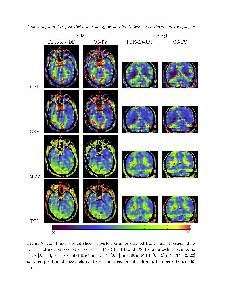
Denoising and Artefact Reduction in Dynamic Flat Detector CT Perfusion Imaging 18
axial coronal
FDK-SR-JBF OS-TV FDK-SR-JBF OS-TV
CBF
CBV
MTT
TTP
X Y
Figure 8: Axial and coronal slices of perfusion maps created from clinical patient data
with head motion reconstructed with FDK-SR-JBF and OS-TV approaches. Windows:
CBF [X = 0, Y = 80] ml/100 g/min; CBV [0, 8] ml/100 g; MTT [0, 12] s; TTP [12, 22]
s. Axial position of slices relative to central slice: (axial) -56 mm; (coronal) -60 to +60
mm.

Denoising and Artefact Reduction in Dynamic Flat Detector CT Perfusion Imaging 19
CBF CBV
Pre Post Pre Post
(ax,cb)
(ax,ol)
(sa)
X Y
Figure 9: Axial (ax) and sagittal (sa) slices of CBF and CBV maps from a patient
study with pre- and post-treatment acquisitions. Axial slices from cerebellum (cb) and
occipital lobes (ol). Map windows pre-treatment acquisition: CBF [X = 0, Y = 80]
ml/100 g/min; CBV [0, 8] ml/100 g. Map windows post-treatment acquisition: CBF [0,
60] ml/100 g/min; CBV [0, 6] ml/100 g. Axial position of the slices relative to central
slice: (ax,cb) -70 mm; (ax,ol) -22 mm; (sa) -72 to +72 mm.
8. Both approaches provide similar visual quality. Also the quantitative results in
Table 4 show similar PC and RMSE distance to the ground truth. However, the
computation time of OS-TV is with 26min 50 s by a factor of more than 23 higher
than the computation time of FDK-SR-JBF with 1min 9 s.
In the TTP and MTT brain phantom maps (Figure 6) the di�erentiation of the
infarct core to the penumbra is lost. The contrast agent enhancement in the infarct core
is very low (peak ∼ 5HU) and therefore the contrast-to-noise (CNR) ratio is accordingly
small. This a�ects the MTT and TTP parameters. As MTT = CBV/CBF, MTT gets
numerically unstable if CBF very small (as in the infarct core). TTP relies on the
detection of the TCC peak, which is di�cult in case of very low CNR. However, the
infarct core can still be depicted from the penumbra by the physician by comparing the
CBV map showing the infarct core to the CBF, MTT, and TTP maps showing the full

Denoising and Artefact Reduction in Dynamic Flat Detector CT Perfusion Imaging 20
MTT TTP
Pre Post Pre Post
(ax,cb)
(ax,ol)
(sa)
X Y
Figure 10: Axial (ax) and sagittal (sa) slices of MTT and TTP maps from a patient
study with pre- and post-treatment acquisitions. Axial slices from cerebellum (cb) and
occipital lobes (ol). Map windows pre-treatment acquisition: MTT [X = 0, Y = 16]
s; TTP [10, 22] s (ol slice) and [14, 28] s (cb slice). Map windows post-treatment
acquisition: MTT [0, 20] s; TTP [11, 25] s. Axial position of the slices relative to
central slice: (ax,cb) -70 mm; (ax,ol) -22 mm; (sa) -72 to +72 mm.
infarct area.
The pre- and post-treatment perfusion maps of the second patient in Figures 9 and
10 provide physiological meaningful results. The pre-treatment maps clearly show a
reduction of CBF and CBV and an increase of MTT and TTP in the left hemisphere
of the cerebellum, which corresponds to the stroke-a�ected area. After successful
recanalization of the cerebellum, the post-treatment maps show increased CBF and CBV
and decreased MTT and TTP in the stroke-a�ected area. This corresponds to hyper-
perfusion, which is a common �nding after recanalization in stroke. Furthermore, the
perfusion maps of the occipital lobes of the brain, which were not a�ected by stroke and
not subject to treatment, look very similar in the pre- and post-treatment maps. This
supports the reproducibility of the proposed acquisition and reconstruction technique.
The FDK-SR-JBF approach produced suitable results in �rst simulation and real

Denoising and Artefact Reduction in Dynamic Flat Detector CT Perfusion Imaging 21
data studies. The perfusion maps allow the physician to determine the infarct area with
the infarct core and the penumbra. Furthermore, the computation speed of FDK-SR-
JBF is su�ciently fast for interventional use on clinical workstations. Therefore it could
be a suitable approach for interventional FD-CTP. However, our heuristic approach can
likely fail to discern streaks and vessels at some voxels and some streak artefacts could
be preserved or small vessels blurred (e.g., see Figure 3d). As long as the artefacts
are limited to few voxels, the image quality of the perfusion maps is impaired, but the
clinical value of the perfusion maps is not strongly a�ected.
One limitation of the evaluated noise and artefact reduction techniques for FD-CTP
is that they can only handle the head motion which occurs between the acquisitions.
Motion during one rotation of the C-arm will cause additional artefacts and might make
the acquired volume unusable for the perfusion computation. Thus including online
motion correction techniques (Debbeler et al. 2013, Wicklein et al. 2012) represents
an important direction for future research. Furthermore, the usage of exact analytical
reconstruction algorithms (Katsevich 2003, Defrise & Clack 1994) could help to improve
the image quality in higher cone beam angles as they avoid the inexact handling of the
cone beam projection data by the Feldkamp short scan algorithm.
5. Conclusions
The simulation and patient studies show the potential of the FDK-SR-JBF approach
for providing viable FD-CTP maps. The FDK-SR-JBF approach produced perfusion
maps with a quality comparable to an algebraic reconstruction technique based on
total variation minimization, but the computation time is reduced by factor of more
than 23 on a clinical workstation. The evaluation using the pre- and post-treatment
acquisitions shows that interventional FD-CTP acquisition is feasible with FDK-SR-JBF
reconstruction. However, further validation of the clinical applicability and robustness
is required by a thorough quantitative comparison of C-arm perfusion maps to CT
perfusion and MR perfusion and will be carried out in the future.
Acknowledgments
The authors gratefully acknowledge funding of the Medical Valley national leading edge
cluster, Erlangen, Germany, diagnostic imaging network, sub-project BD 16, research
grant nr. 13EX1212G. M. Manhart gratefully acknowledges funding from Siemens AG,
Angiography & Interventional X-Ray Systems, Germany. Y. Deuerling-Zheng and M.
Kowarschik are employed by Siemens AG, Healthcare Sector, Germany.
Disclaimer: The concepts and information presented in this paper are based on
research and are not commercially available. The patient study has been approved
by the ethics commission of the Medical Faculty at Friedrich-Alexander-Universität
Erlangen-Nürnberg, Germany, Ethik-No. 4535 on Dec 14th 2011.

Denoising and Artefact Reduction in Dynamic Flat Detector CT Perfusion Imaging 22
References
Ahmed A S, Zellerho� M, Strother C, Pulfer K, Deuerling-Zheng Y, Redel T, Royalty K, Consigny D
& Niemann D 2009 C-arm CT measurement of cerebral blood volume: An experimental study
in canines AJNR 30(5), 917�22.
Aichert A, Manhart M T, Navalpakkam B K, Grimm R, Hutter J, Maier A, Hornegger J & Doer�er
A 2013 A realistic digital phantom for perfusion C-arm CT based on MRI data in `Proc. IEEE
NSS MIC 2013'. (accepted for presentation).
Aurich V &Weule J 1995 in G Sagerer, S Posch & F Kummert, eds, `Mustererkennung 1995' Informatik
aktuell Springer Berlin Heidelberg pp. 538�545.
http://dx.doi.org/10.1007/978-3-642-79980-8_63
Dale A M, Fischl B & Sereno M I 1999 Cortical surface-based analysis: I. Segmentation and surface
reconstruction NeuroImage 9(2), 179�194.
Debbeler C, Maass N, Elter M, Dennerlein F & Buzug T M 2013 A new CT rawdata redundancy
measure applied to automated misalignment correction in `Proc. 12th International Meeting on
Fully Three-Dimensional Image Reconstruction in Radiology and Nuclear Medicine' Tahoe City,
CA, USA pp. 264�267.
Defrise M & Clack R 1994 A cone-beam reconstruction algorithm using shift-variant �ltering and
cone-beam backprojection Medical Imaging, IEEE Transactions on 13(1), 186�195.
Feldkamp L, Davis L & Kress J 1984 Practical cone-beam algorithm Journal of the Optical Society of
America A 1(6), 612�619.
Fieselmann A, Ganguly A, Deuerling-Zheng Y, Zellerho� M, Rohkohl C, Boese J, Hornegger J & Fahrig
R 2012 Interventional 4-D C-arm CT perfusion imaging using interleaved scanning and partial
reconstruction interpolation Medical Imaging, IEEE Transactions on 31(4), 892 � 906.
Fieselmann A, Kowarschik M, Ganguly A, Hornegger J & Fahrig R 2011 `Deconvolution-based CT and
MR brain perfusion measurement: Theoretical model revisited and practical implementation
details' International Journal of Biomedical Imaging. Article ID 467563.
Furlan A, Higashida R, Wechsler L, Gent M, Rowley H, Kase C, Pessin M, Ahuja A, Callahan F, Clark
WM et al. 1999 Intra-arterial prourokinase for acute ischemic stroke JAMA 282(21), 2003�2011.
Hacke W, Kaste M, Bluhmki E, Brozman M, Dávalos A, Guidetti D, Larrue V, Lees K R, Medeghri
Z, Machnig T et al. 2008 Thrombolysis with alteplase 3 to 4.5 hours after acute ischemic stroke
New England Journal of Medicine 359(13), 1317�1329.
Katsevich A 2003 A general scheme for constructing inversion algorithms for cone beam ct International
Journal of Mathematics and Mathematical Sciences 2003(21), 1305�1321.
Manhart M T, Aichert A, Kowarschik M, Deuerling-Zheng Y, Stru�ert T, Doer�er A, Maier A K &
Hornegger J 2013 Guided noise reduction with streak removal for high speed perfusion C-arm
CT in `Proc. IEEE NSS MIC 2013'. (accepted for presentation).
Manhart M T, Fieselmann A, Deuerling-Zheng Y & Kowarschik M 2013 Iterative denoising algorithms
for perfusion C-arm CT with a rapid scanning protocol in `Proc. IEEE ISBI 2013' San Francisco,
CA, USA pp. 1223�1227.
Manhart M T, Kowarschik M, Fieselmann A, Deuerling-Zheng Y, Royalty K, Maier A K & Hornegger
J 2013 Dynamic iterative reconstruction for interventional 4-D C-arm CT perfusion imaging
Medical Imaging, IEEE Transactions on 32(7), 1336�1348.
Mendrik A M, Vonken E, van Ginneken B, de Jong H W, Riordan A, van Seeters T, Smit E J, Viergever
M A & Prokop M 2011 TIPS bilateral noise reduction in 4D CT perfusion scans produces high-
quality cerebral blood �ow maps Physics in Medicine and Biology 56(13), 3857�3872.
Miles K A & Gri�ths M R 2003 Perfusion CT: a worthwhile enhancement? British Journal of Radiology
76(904), 220�231.
Navalpakkam B K, Braun H, Kuwert T & Quick H H 2013 Magnetic Resonance-Based Attenuation
Correction for PET/MR Hybrid Imaging Using Continuous Valued Attenuation Maps Invest
Radiol 48(5), 323�332.

Denoising and Artefact Reduction in Dynamic Flat Detector CT Perfusion Imaging 23
Neukirchen C, Giordano M & Wiesner S 2010 An iterative method for tomographic X-ray perfusion
estimation in a decomposition model-based approach Medical Physics 37(12), 6125�6141.
Parker D L 1982 Optimal short scan convolution reconstruction for fan beam CT Medical Physics
9(2), 254�257.
Petschnigg G, Szeliski R, Agrawala M, Cohen M, Hoppe H & Toyama K 2004 Digital photography with
�ash and no-�ash image pairs ACM Transactions on Graphics (TOG) 23(3), 664�672.
Rha J H & Saver J L 2007 The impact of recanalization on ischemic stroke outcome a meta-analysis
Stroke 38(3), 967�973.
Riordan A J, Prokop M, Viergever M A, Dankbaar J W, Smit E J & de Jong H W A M 2011
Validation of CT brain perfusion methods using a realistic dynamic head phantom Medical
Physics 38(6), 3212�3221.
Ritschl L, Bergner F, Fleischmann C & Kachelrieÿ M 2011 Improved total variation-based CT image
reconstruction applied to clinical data Physics in Medicine and Biology 56(6), 1545�1561.
Royalty K, Manhart M, Pulfer K, Deuerling-Zheng Y, Strother C, Fieselmann A & Consigny D 2013 C-
arm CT measurement of cerebral blood volume and cerebral blood �ow using a novel high-speed
acquisition and a single intravenous contrast injection AJNR -, �. (in press).
Savitzky A & Golay M J E 1964 Smoothing and di�erentiation of data by simpli�ed least squares
procedures Analytical Chemistry 36(8), 1627�1639.
Shepp L A & Logan B F 1974 The Fourier reconstruction of a head section Nuclear Science, IEEE
Transactions on 21(3), 21�43.
Østergaard L, Weissko� R M, Chesler, David A. Gyldensted C & Rosen B R 1996 High resolution
measurement of cerebral blood �ow using intravascular tracer bolus passages. Part I:
Mathematical approach and statistical analysis Magnetic Resonance in Medicine 36(5), 715�
725.
Stru�ert T, Deuerling-Zheng Y, Engelhorn T, Kloska S, Gölitz P, Köhrmann M, Schwab S, Strother
C & Doer�er A 2012 Feasibility of cerebral blood volume mapping by �at panel detector CT in
the angiography suite: �rst experience in patients with acute middle cerebral artery occlusions
American Journal of Neuroradiology 33(4), 618�625.
Stru�ert T, Deuerling-Zheng Y, Kloska S, Engelhorn T, Boese J, Zellerho� M, Schwab S & Doer�er A
2011 Cerebral blood volume imaging by �at detector computed tomography in comparison to
conventional multislice perfusion CT European Radiology 21(4), 882�889.
Stru�ert T, Deuerling-Zheng Y, Kloska S, Engelhorn T, Strother C, Kalender W, Köhrmann M, Schwab
S & Doer�er A 2010 Flat detector CT in the evaluation of brain parenchyma, intracranial
vasculature, and cerebral blood volume: a pilot study in patients with acute symptoms of
cerebral ischemia American Journal of Neuroradiology 31(8), 1462�1469.
Stru�ert T, Richter G, Engelhorn T, Doelken M, Goelitz P, Kalender W A, Ganslandt O & Doer�er A
2009 Visualisation of intracerebral haemorrhage with �at-detector CT compared to multislice
CT: results in 44 cases European radiology 19(3), 619�625.
Tomasi C & Manduchi R 1998 Bilateral �ltering for gray and color images in `Computer Vision, Sixth
International Conference on' IEEE Washington, DC, USA pp. 839�846.
Viola P & Wells III W M 1997 Alignment by maximization of mutual information International Journal
of Computer Vision 24(2), 137�154.
Wagner M, Deuerling-Zheng Y, Möhlenbruch M, Bendszus M, Boese J & Heiland S 2013 A model
based algorithm for perfusion estimation in interventional C-arm CT systems Medical Physics
40(3), 0319161�03191611.
Wicklein J, Kunze H, Kalender W A & Kyriakou Y 2012 Image features for misalignment correction
in medical �at-detector CT Medical Physics 39, 4918.
Wiesent K, Barth K, Navab N, Durlak P, Brunner T, Schuetz O & Seissler W 2000 Enhanced 3-
d-reconstruction algorithm for c-arm systems suitable for interventional procedures Medical
Imaging, IEEE Transactions on 19(5), 391�403.
Zaidat O O, Wolfe T, Hussain S I, Lynch J R, Gupta R, Delap J, Torbey M T & Fitzsimmons B F

Denoising and Artefact Reduction in Dynamic Flat Detector CT Perfusion Imaging 24
2008 Interventional acute ischemic stroke therapy with intracranial self-expanding stent Stroke
39(8), 2392�2395.


