Machine Learning Srihari
Deep LearningSargur Srihari
1
Machine Learning Srihari
Topics
• Multilayer Neural Networks• Deep Convolutional Nets• Recurrent Nets• Deep Belief Networks
2
Machine Learning Srihari
Deep Learning Summary (LeCun,Bengio,Hinton, Nature 2015)
1. Computational models composed of multiple processing layers• To learn representations of data with multiple levels of abstraction
2. Dramatically improved state-of-the-art in:• Speech recognition, Visual object recognition, Object detection• Other domains: Drug discovery, Genomics
3. Discovers intricate structure in large data sets• Using backpropagation to change parameters• Compute representation in each layer from previous layer
4. Deep convolutional nets: image proc, video, speech5. Recurrent nets: sequential data, e,g., text, speech
3
Machine Learning Srihari
ML Technology
• ML powers many aspects of modern society• Web searches• Content filtering on social networks• Recommendations on e-commerce websites• Consumer products:
• cameras, smartphones• ML used to:
• Identify objects in images• Transcribe speech to text• Match news items, posts or products with user interests• Select relevant results of search
• Increasingly these use deep learning techniques 4
Machine Learning Srihari
Limitations of Conventional ML
• Limited in ability to process natural data in raw form• PR and ML systems require
• careful engineering and domain expertise to transform raw data, e.g., pixel values, into a feature vector for a classifier
5
Machine Learning Srihari
Representation learning
• Methods that allow a machine to be fed with raw data to automatically discover representations needed for detection or classification
• Deep Learning methods are Representation Learning Methods
• Use multiple levels of representation• Composing simple but non-linear modules that transform
representation at one level (starting with raw input) into a representation a ta higher slightly more abstract level
• Complex functions can be learned• Higher layers of representation amplify aspects of input
important for discrimination and suppress irrelevant variations
6
Machine Learning Srihari
Image Example• Input is an array of pixel values
• First stage is presence or absence of edges at particular locations and orientations of image
• Second layer detects motifs by spotting particular arrangements of edges, regardless of small variations in edge positions
• Third layer assembles motifs into larger combinations that corresponds to parts of familiar objects
• Subsequent layers would detect objects as combinations of these parts
• Key aspect of deep learning: • These layers of features are not designed by human engineers• They are learned from data using a general purpose learning
procedure
7
Machine Learning Srihari
Applications of Deep Learning
• Major advances in solving problems that have resisted best attempts of AI for many years
• Good at discovering structures in high-dimensional data• Many domains of science, government and business
• Beaten other ML techniques at:• Predicting activity of potential drug molecules• Analysing particle accelerator data• Reconstructing brain circuits• Predicting effects of mutations in non-coding DNA on gene
expression and disease• Produced promising results for NLP
• Topic categorization, sentiment analysis, QA, MT8

Machine Learning Srihari
Supervised Learning
• Most common form of ML, deep or not• Ex: classify images containing a house, a car, a person or a pet• Collect large data set of images of houses, cars, people and pets,
each labelled with its category• During training, machine is shown image and it produces an
output in the form of a vector of scores, one for each category• We want desired category to have highest score– which is
unlikely before training• Compute objective function that measures error between
output scores and desired scores• Modify internal parameters to reduce error• In deep learning hundreds of millions of adjustable
weights and hundreds of millions of labelled examples9
Machine Learning Srihari
Gradient Descent
• Objective function, averaged over all training examples is a hilly landscape in high-dimensional space of weight values
• Negative gradient vector indicates direction of steepest descent taking it closer to a minimum
10
Machine Learning Srihari
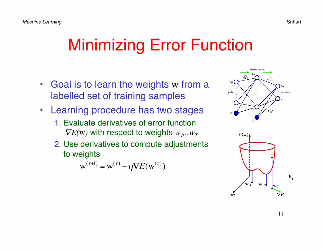
Minimizing Error Function
• Goal is to learn the weights w from a labelled set of training samples
• Learning procedure has two stages1. Evaluate derivatives of error function ∇E(w) with respect to weights w1,..wT
2. Use derivatives to compute adjustments to weights
11
w(τ+1) =w(τ ) −η∇E(w(τ ) )

Machine Learning Srihari
Using derivatives to update weights• Gradient descent
• Update the weights using
• Where the gradient vector consists of the vector of derivatives evaluated using back-propagation
12
w(τ+1) = w(τ)− η∇E (w(τ))
∇E (w(τ))
∇E(w) =ddw
E(w) =
∂E∂w
11(1)
.∂E∂w
MD(1)
∂E∂w
11(2)
.∂E∂w
KM(2)
⎡
⎣
⎢⎢⎢⎢⎢⎢⎢⎢⎢⎢⎢⎢⎢⎢⎢⎢⎢⎢⎢⎢
⎤
⎦
⎥⎥⎥⎥⎥⎥⎥⎥⎥⎥⎥⎥⎥⎥⎥⎥⎥⎥⎥⎥
There are W= M(D+1)+K(M+1) elements in the vector Gradient is a W x 1 vector ∇E (w(τ))
Machine Learning Srihari
Stochastic Gradient Descent (SGD)
13
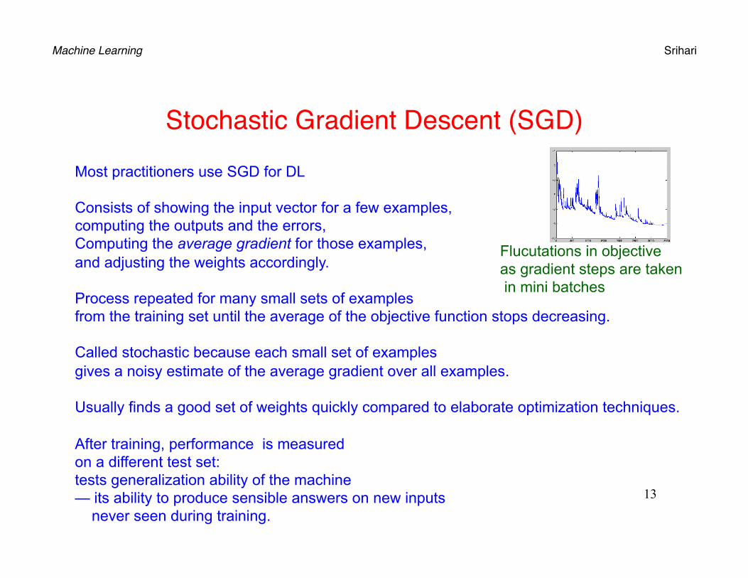
Most practitioners use SGD for DL Consists of showing the input vector for a few examples, computing the outputs and the errors, Computing the average gradient for those examples, and adjusting the weights accordingly. Process repeated for many small sets of examples from the training set until the average of the objective function stops decreasing. Called stochastic because each small set of examples gives a noisy estimate of the average gradient over all examples. Usually finds a good set of weights quickly compared to elaborate optimization techniques. After training, performance is measured on a different test set: tests generalization ability of the machine — its ability to produce sensible answers on new inputs never seen during training.
Flucutations in objective as gradient steps are taken in mini batches
Machine Learning Srihari
3. Backpropagate the δ’s using
to obtain δj for each hidden unit
4. Use
to evaluate required derivatives
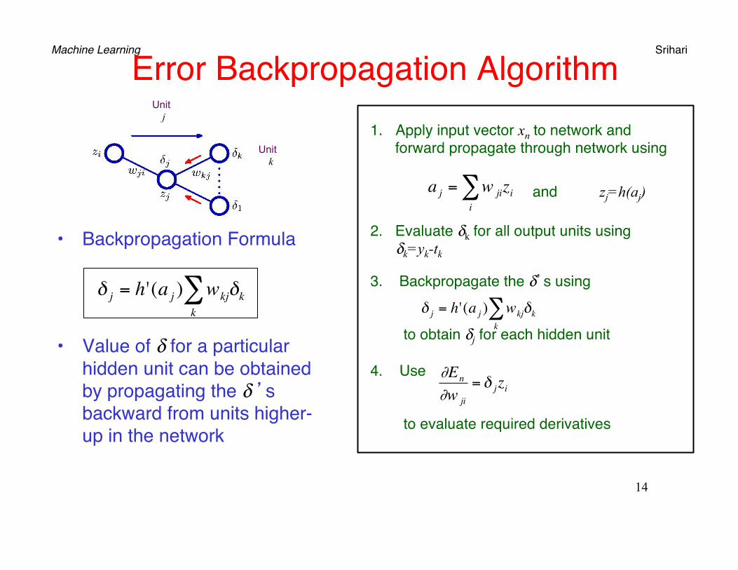
Error Backpropagation Algorithm
• Backpropagation Formula
• Value of δ for a particular hidden unit can be obtained by propagating the δ ’s backward from units higher-up in the network
14
€
δ j = h'(a j ) wkjk∑ δk
1. Apply input vector xn to network and forward propagate through network using
€
a j = w jii∑ zi and zj=h(aj)
2. Evaluate δk for all output units using δk=yk-tk
€
δ j = h'(a j ) wkjk∑ δk
€
∂En
∂w ji
= δ j zi
Unit j
Unit k
Machine Learning Srihari
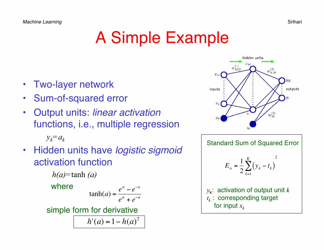
A Simple Example
• Two-layer network• Sum-of-squared error• Output units: linear activation
functions, i.e., multiple regression yk=ak
• Hidden units have logistic sigmoid activation function
h(a)=tanh (a) where
simple form for derivative
€
tanh(a) =ea − e−a
ea + e−a
€
h'(a) =1− h(a)2
Standard Sum of Squared Error
yk: activation of output unit k tk : corresponding target for input xk
€
En =12
yk − tk( )k=1
K
∑2
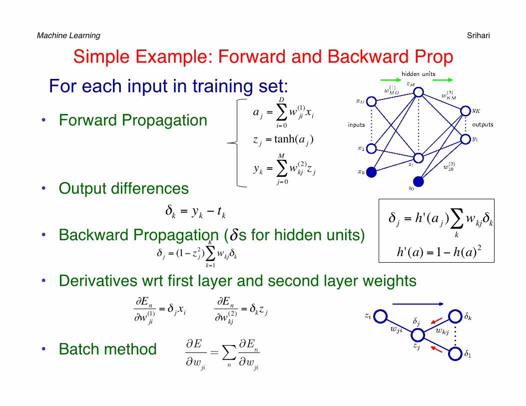
Machine Learning Srihari Simple Example: Forward and Backward Prop
• Forward Propagation
• Output differences
• Backward Propagation (δ s for hidden units)
• Derivatives wrt first layer and second layer weights
• Batch method
€
a j = w ji(1)
i= 0
D
∑ xi
z j = tanh(a j )
yk = wkj(2)
j= 0
M
∑ z j
€
δk = yk − tk
€
δ j = (1− z j2) wkjδk
k=1
K
∑
€
∂En
∂w ji(1) = δ j xi
∂En
∂wkj(2) = δkz j
For each input in training set:
€
h'(a) =1− h(a)2
€
δ j = h'(a j ) wkjk∑ δk
∂E
∂wji
=∂E
n
∂wjin
∑
Machine Learning Srihari
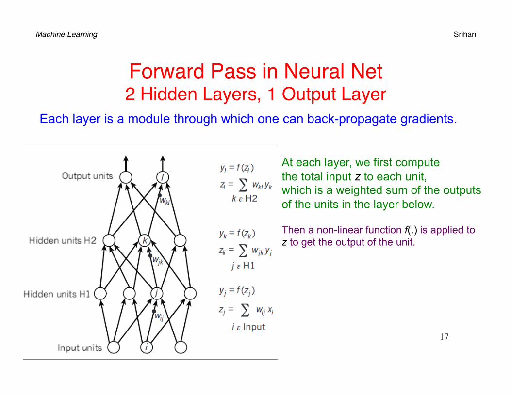
Forward Pass in Neural Net2 Hidden Layers, 1 Output Layer
17
At each layer, we first compute the total input z to each unit, which is a weighted sum of the outputs of the units in the layer below. Then a non-linear function f(.) is applied to z to get the output of the unit.
Each layer is a module through which one can back-propagate gradients.
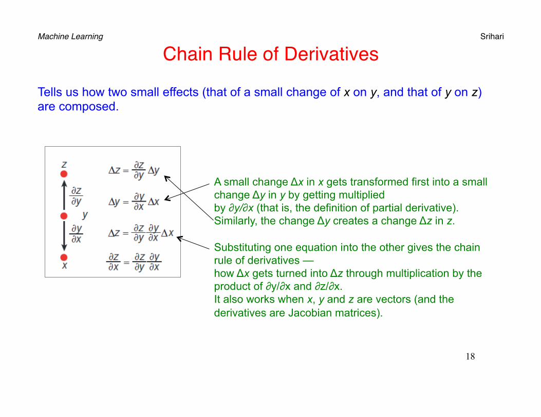
Machine Learning Srihari Chain Rule of Derivatives
18
A small change Δx in x gets transformed first into a small change Δy in y by getting multiplied by ∂y/∂x (that is, the definition of partial derivative). Similarly, the change Δy creates a change Δz in z. Substituting one equation into the other gives the chain rule of derivatives — how Δx gets turned into Δz through multiplication by the product of ∂y/∂x and ∂z/∂x. It also works when x, y and z are vectors (and the derivatives are Jacobian matrices).
Tells us how two small effects (that of a small change of x on y, and that of y on z) are composed.

Machine Learning Srihari
Equations for Computing the Backward Pass
19
Two hidden layers Layers are labelled i,j,k,l At each hidden layer we compute the error derivative wrt the output of each unit, which is a weighted sum of the error derivatives wrt the total inputs to the units in the layer above. Convert error derivative wrt the output into the error derivative wrt the input by multiplying it by the gradient of f(z). At the output layer, the error derivative wrt the output of a unit is computed by differentiating the cost function. This gives yl − tl if the cost function for unit l is 0.5(yl − tl
)2, where tl is the target value. Once the ∂E/∂zk is known, the error-derivative for the weight wjk on the connection from unit j in the layer below is just yj ∂E/∂zk.
Machine Learning Srihari
Choice of non-linear function
• Most popular today is Rectified Linear Unit (ReLU)• a half-wave rectifier
f(z)=max(z,0) • In past decades, neural nets used smoother non-
linearitiestanh(z) or 1/(1+exp(-z))
• ReLU learns faster in networks with many layers• Allowing training of deep supervised network without
unsupervised pre-training
20

Machine Learning Srihari
Nonlinear Functions used in Neural Nets
21
• Rectified linear unit (ReLU) f(z) = max(0,z) commonly used in recent years,
• More conventional sigmoids:
• hyberbolic tangent, f(z) = (exp(z) − exp(−z))/(exp(z) + exp(−z)) and
• logistic function, f(z) = 1/(1 + exp(−z))

Machine Learning Srihari
Neural Network with 2 Inputs, 2 HiddenUnits, 1 Output unit
22
• Input Data (red and blue curves) are not linearly separable • Network makes them linearly separable
• By distorting the input space • Note that grid is also distorted
x1
x2
x1 x2
y1
y2
z
Machine Learning Srihari
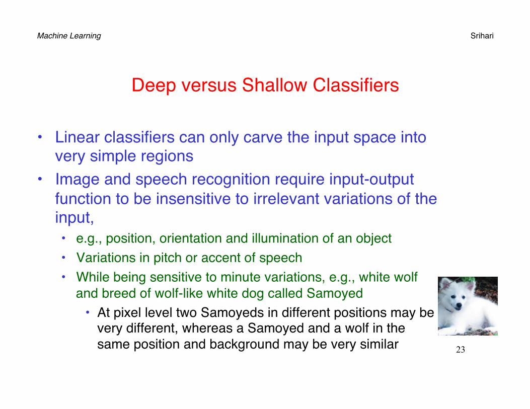
Deep versus Shallow Classifiers
• Linear classifiers can only carve the input space into very simple regions
• Image and speech recognition require input-output function to be insensitive to irrelevant variations of the input, • e.g., position, orientation and illumination of an object• Variations in pitch or accent of speech• While being sensitive to minute variations, e.g., white wolf
and breed of wolf-like white dog called Samoyed• At pixel level two Samoyeds in different positions may be
very different, whereas a Samoyed and a wolf in the same position and background may be very similar 23
Machine Learning Srihari
Selectivity-Invariance dilemma
• Shallow classifiers need a good feature extractor• One that produces representations that are:
• selective to aspects of image important for discrimination • but invariant to irrelevant aspects such as pose of the animal
• Generic features (e.g., Gaussian kernel) do not generalize well far from training examples
• Hand-designing good feature extractors requires engineering skill and domain expertise
• Deep learning learns features automatically
24
Machine Learning Srihari
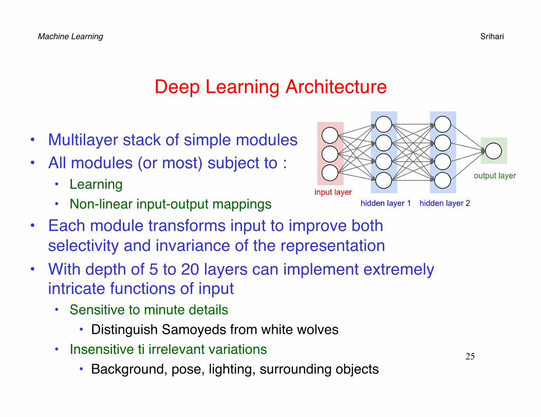
Deep Learning Architecture
• Multilayer stack of simple modules• All modules (or most) subject to :
• Learning• Non-linear input-output mappings
• Each module transforms input to improve both selectivity and invariance of the representation
• With depth of 5 to 20 layers can implement extremely intricate functions of input• Sensitive to minute details
• Distinguish Samoyeds from white wolves• Insensitive ti irrelevant variations
• Background, pose, lighting, surrounding objects25
Machine Learning Srihari
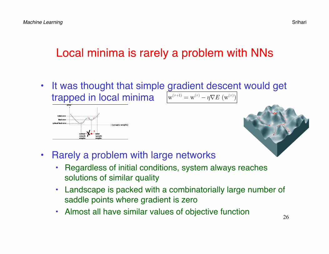
Local minima is rarely a problem with NNs
• It was thought that simple gradient descent would get trapped in local minima
• Rarely a problem with large networks• Regardless of initial conditions, system always reaches
solutions of similar quality• Landscape is packed with a combinatorially large number of
saddle points where gradient is zero• Almost all have similar values of objective function
26
w(τ+1) = w(τ)− η∇E (w(τ))

Machine Learning Srihari
Pre-training• Unsupervised learning to create layers of feature
detectors• No need for labelled data
• Objective of learning in each layer of feature detectors:• Ability to reconstruct or model activities of feature detectors
(or raw inputs) in layer below• By pre-training weights of a deep network could be initialized
to sensible values• Final layer of output units added at top of network
and whole deep system fine-tuned using back-propagation
• Worked well in handwritten digit recognition• When data was limited
27
Machine Learning Srihari
Pre-training in Speech Recognition
• First major application was in speech recognition• Made possible by advent of fast GPUs
• Allowed networks to be trained 10 or 20 times faster• Record-breaking results on speech reco benchmark
28

Machine Learning Srihari
From pre-training to ConvNets
• It turned out that pre-training stage was only needed for small data sets
• Convolutional neural networks• Type of deep feedforward network • Much easier to train and generalized much better than
networks with full connectivity between adjacent layers
29
Machine Learning Srihari
Convolutional Neural Networks
• Designed to process data that come in the form of multiple arrays• E.g., a color image composed of three 2D arrays of pixel
intensities in three color channels• Many data modalities are in the form of multiple
arrays:• 1D for signals and sequences, including language• 2D for images and audio spectrograms• 3D for video or volumetric images
30

Machine Learning Srihari
Four key ideas behind ConvNets
• Take advantage of properties of natural signals1. Local connections2. Shared weights3. Pooling4. Use of many layers
31
Machine Learning Srihari
Limitations of Neural Networks
• Need substantial number of training samples• Slow learning (convergence times)• Inadequate parameter selection techniques that lead
to poor minima
32
Machine Learning Srihari
Solution: Exploitation of Local Properties
• Network should exhibit invariance to translation, scaling and elastic deformations• A large training set can take care of this
• It ignores a key property of images• Nearby pixels are more strongly correlated than distant ones• Modern computer vision approaches exploit this property
• Information can be merged at later stages to get higher order features and about whole image
33
Machine Learning Srihari
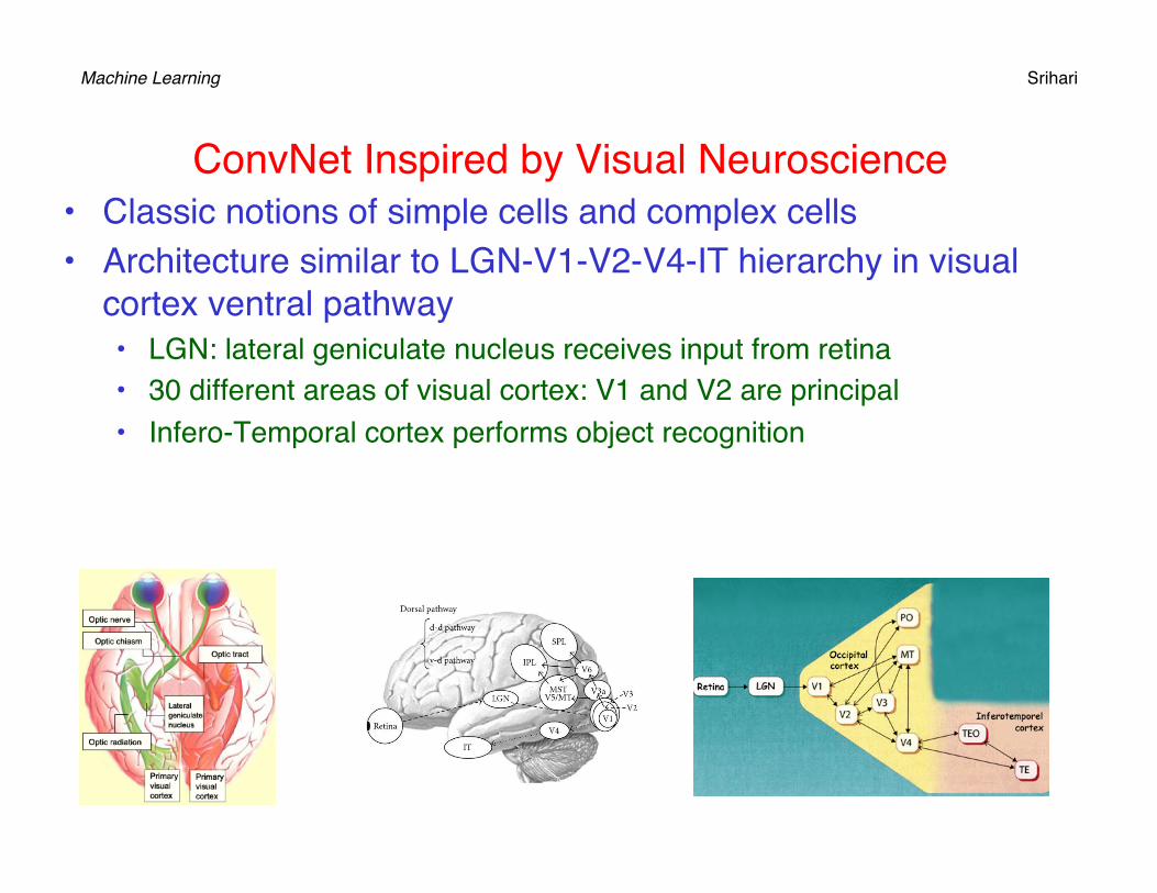
ConvNet Inspired by Visual Neuroscience• Classic notions of simple cells and complex cells • Architecture similar to LGN-V1-V2-V4-IT hierarchy in visual
cortex ventral pathway• LGN: lateral geniculate nucleus receives input from retina• 30 different areas of visual cortex: V1 and V2 are principal• Infero-Temporal cortex performs object recognition
34
Machine Learning Srihari
Three Mechanisms of Convolutional Neural Networks
1. Local Receptive Fields2. Subsampling3. Weight Sharing
35
Machine Learning Srihari Convolution and Sub-sampling
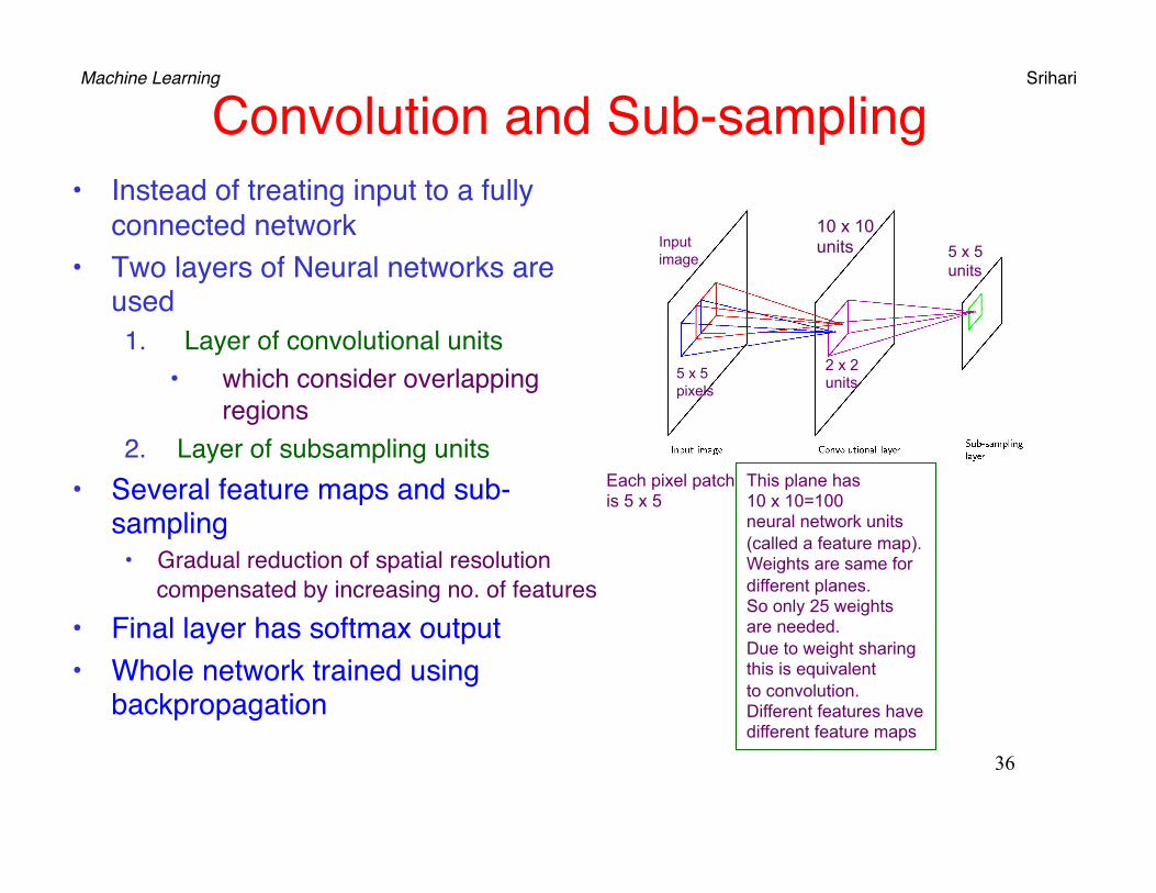
• Instead of treating input to a fully connected network
• Two layers of Neural networks are used1. Layer of convolutional units
• which consider overlapping regions
2. Layer of subsampling units• Several feature maps and sub-
sampling• Gradual reduction of spatial resolution
compensated by increasing no. of features• Final layer has softmax output• Whole network trained using
backpropagation
36
Each pixel patch is 5 x 5
This plane has 10 x 10=100 neural network units (called a feature map). Weights are same for different planes. So only 25 weights are needed. Due to weight sharing this is equivalent to convolution. Different features have different feature maps
10 x 10 units
5 x 5 pixels
2 x 2 units
Input image 5 x 5
units
Machine Learning Srihari
Soft weight sharing
• Reducing the complexity of a network• Encouraging groups of weights to have similar values• Only applicable when form of the network can be
specified in advance• Division of weights into groups, mean weight value
for each group and spread of values are determined during the learning process
37
Machine Learning Srihari
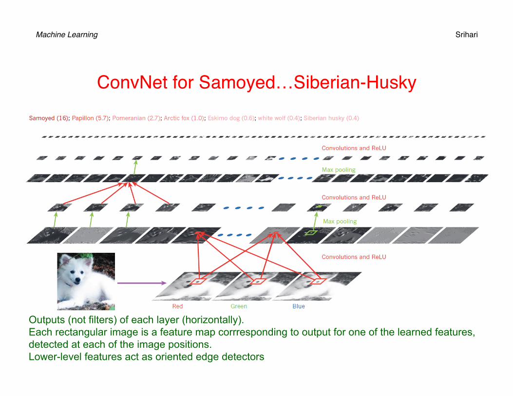
ConvNet for Samoyed…Siberian-Husky
Outputs (not filters) of each layer (horizontally). Each rectangular image is a feature map corrresponding to output for one of the learned features, detected at each of the image positions. Lower-level features act as oriented edge detectors
Machine Learning Srihari
Architecture of a typical ConvNet
• Structured as a series of stages• First few stages are composed of two types of layers and
a non-linearity:1. Convolutional layer
• To detect local conjunctions of features from previous layer2. Non-linearity
• ReLU3. Pooling layer
• To merge semantically similar features into one
39
Machine Learning Srihari
A convolutional layer unit
• Organized in feature maps• Each unit connected to local patches in feature maps
of previous layer through weights (called a filter bank)• Result is passed through a ReLU
40
Machine Learning Srihari
A pooling layer unit
• Computes maximum of a local patch of units in one feature map
• Neighboring pooling units take input from patches that are shifted by more than one row or column• Thereby reducing the dimension of the representation• Creating invariance to small shifts and distortions
41
Machine Learning Srihari
Backpropagation of Gradients through ConvNet
• As simple as through a regular deep network• Allow all weights in all filter banks to be trained
42
Machine Learning Srihari
ConvNet History
• Neocognitron• Similar architecture• Did not have end-to-end supervised learning using Backprop
• ConvNet with probabilistic model was used for OCR and handwritten check reading
43

Machine Learning Srihari
Applications of ConvNets
• Applied with great success to images: detection, segmentation and recognition of objects and regions• Tasks where abundant data was available
• Traffic sign recognition• Segmentation of biological images
• Connectomics • Detection of faces, text, pedestrians, human bodies in natural images• Major recent practical success is face recognition
• Images can be labeled at pixel level• Applications in autonomous mobile robots, and self-driving cars
• Other applications gaining importance• Natural language understanding• Speech recognition
Machine Learning Srihari
Success of ConvNet in ImageNet Competition 2012
• Data set of 1 million images from the web• Contained 1,000 different classes• Error rate
• Halved the error rate of best competing computer vision approaches• Success came from:
• Efficient use of GPUs• ReLUs• New regularization technique called dropout• Techniques to generate new training samples by deforming existing ones
45
Machine Learning Srihari
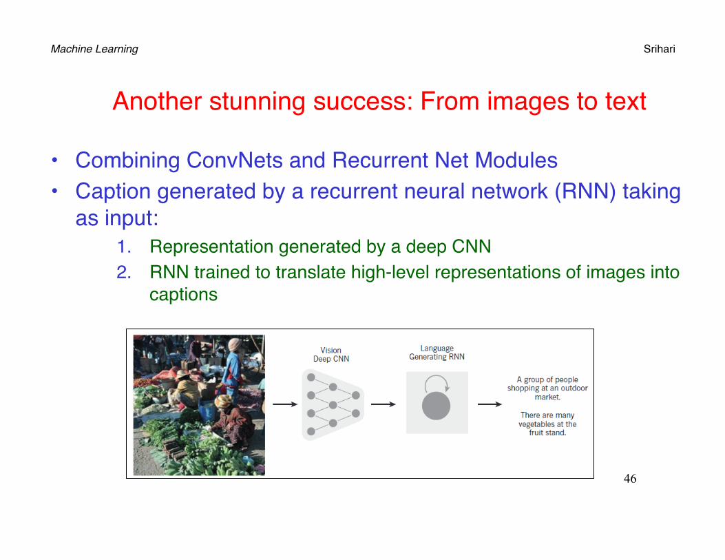
Another stunning success: From images to text
• Combining ConvNets and Recurrent Net Modules• Caption generated by a recurrent neural network (RNN) taking
as input:1. Representation generated by a deep CNN2. RNN trained to translate high-level representations of images into
captions
46
Machine Learning Srihari
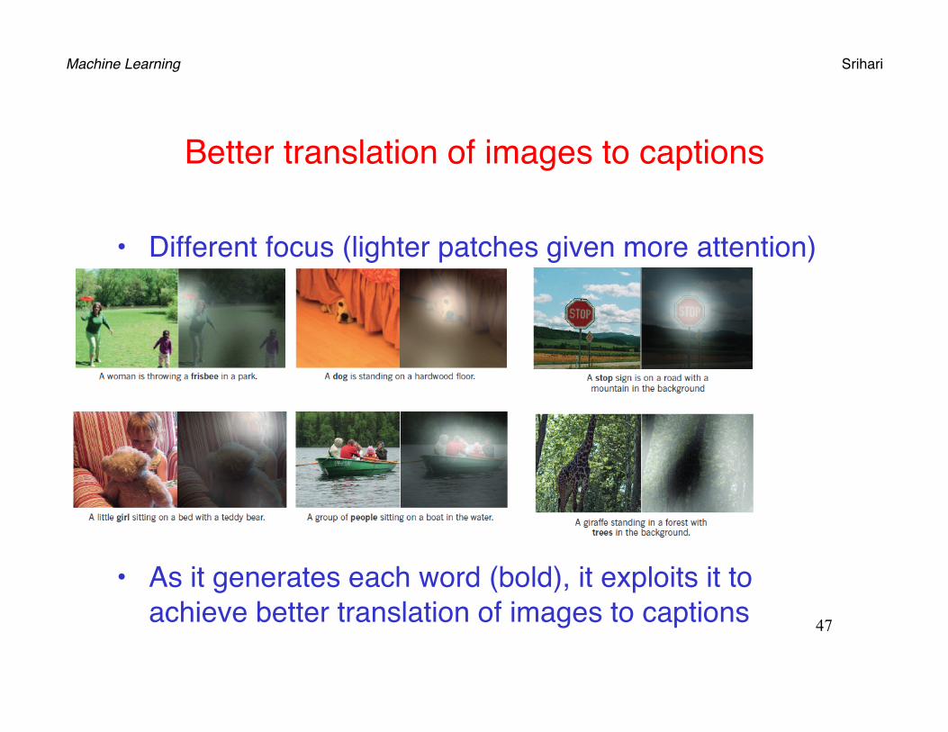
Better translation of images to captions
• Different focus (lighter patches given more attention)
• As it generates each word (bold), it exploits it to achieve better translation of images to captions 47
Machine Learning Srihari
Recent ConvNet architectures
1. 10 to 20 layers of ReLUs2. Hundreds of millions of weights3. Billions of connections between units4. Training time
• Would have taken weeks a couple of years ago• Advances in hardware, software and parallelization reduces
it to a few hours• ConvNets are easily amenable to efficient hardware
implementations• NVIDIA, Mobileye, Intel, Qualcomm and Samsung are
developing ConvNet chips for smartphones, cameras, robots and self-driving cars
Machine Learning Srihari
Distributed Representations
• Deep nets have two different exponential advantages over classic learning algorithms. Both advantages arise from • power of composition• Depend on underlying data-generating distribution having an
appropriate compositional structure1. Learning distributed representations enable
generalization to new combinations of the values of learned features beyond those seen during training1. E.g., 2n combinations are possible with n binary features
2. Composing layers of representations brings another advantage: exponential in depth 49

Machine Learning Srihari
Language Processing: Prediction• Predicting the next word from local context of earlier words
• Each word presented as a 1-of-N vector• In the first layer each word creates a different word vector• In the language model, other next layers learn to convert input
word vector to output word vector for the predicted word
50
Words Phrases Word representation for modeling language, non-linearly projected to 2-D using t-SNE algorithm. Semantically similar words are mapped nearby.
2-D representation of phrases learnt by English-French encoder-decoder learnt by RNN
Learnt using backpropagation that jointly learns representation for each word and function that predicts a target quantity (next word or sequence of words for translation)
Machine Learning Srihari
Logic-inspired vs Neural network-inspired paradigms
• Logic-inspired paradigm uses• Instance of a symbol is something for which the only
property is that is either identical or non-identical to other symbol instances
• It has no internal structure relevant to its use• To reason with symbols they must be bound to variables in
judiciously chosen rules of inference• Neural networks use
• big activity vectors, big weight matrices and scalar non-linearities
• to perform fast intuitive inference that underpins commonsense reasoning
51
Machine Learning Srihari
N-gram vs Neural Language Models
• Standard statistical models count frequencies of short symbol sequences of length upto N
• No of possible sequences is VN, where V is vocabulary size
• So taking context of more than a handful of words would require very large corpora
• N-grams treat each word as an atomic unit, so they cannot generalize across semantically related sequences
• Neural models can because they associate each word with a vector of real-valued features 52
Machine Learning Srihari
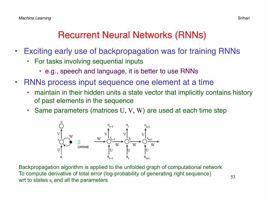
Recurrent Neural Networks (RNNs)• Exciting early use of backpropagation was for training RNNs
• For tasks involving sequential inputs• e.g., speech and language, it is better to use RNNs
• RNNs process input sequence one element at a time • maintain in their hidden units a state vector that implicitly contains history
of past elements in the sequence• Same parameters (matrices U, V, W) are used at each time step
53
Backpropagation algorithm is applied to the unfolded graph of computational network To compute derivative of total error (log-probability of generating right sequence) wrt to states si and all the parameters

Machine Learning Srihari
Deep Belief Networks
• DBNs are Generative Models• Provide estimates of both p(x|Ck) and p(Ck|x)
• Conventional neural networks are discriminative• Directly estimate p(Ck|x)
• Consist of several layers of Restricted Boltzmann Machines (RBM)
• RBM• A form of Markov Random Field
54

Machine Learning Srihari
Deep Belief Network Framework
55
Machine Learning Srihari
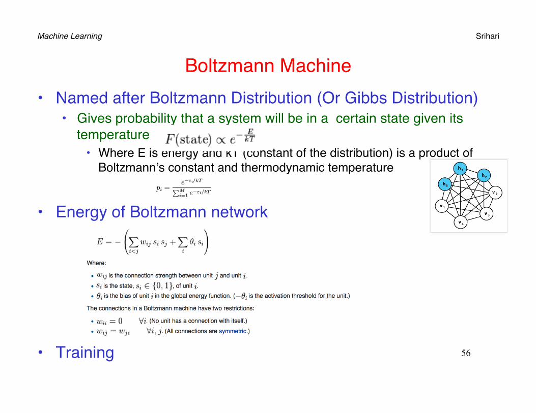
Boltzmann Machine• Named after Boltzmann Distribution (Or Gibbs Distribution)
• Gives probability that a system will be in a certain state given its temperature
• Where E is energy and kT (constant of the distribution) is a product of Boltzmann’s constant and thermodynamic temperature
• Energy of Boltzmann network
• Training 56
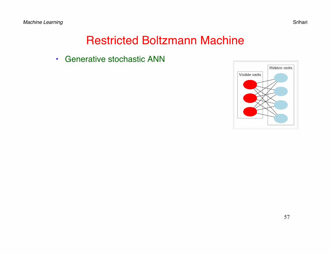
Machine Learning Srihari
Restricted Boltzmann Machine• Generative stochastic ANN
57


