
Working Paper No. 588
Decomposition of the Black-White Wage Differentialin the Physician Market
by
Tsu-Yu Tsao and Andrew PearlmanBard College
March 2010
* We gratefully acknowledge the financial support provided by the Bard Research Fund.We also thank two anonymous evaluators of our Bard Research Fund proposal for manyhelpful comments and suggestions, and Anh Pham, Michael Smith, and DobromiraTrendafilova for research assistance. All errors are our own.
The Levy Economics Institute Working Paper Collection presents research in progress byLevy Institute scholars and conference participants. The purpose of the series is todisseminate ideas to and elicit comments from academics and professionals.
The Levy Economics Institute of Bard College, founded in 1986, is a nonprofit,nonpartisan, independently funded research organization devoted to public service.Through scholarship and economic research it generates viable, effective public policyresponses to important economic problems that profoundly affect the quality of life inthe United States and abroad.
Levy Economics InstituteP.O. Box 5000
Annandale-on-Hudson, NY 12504-5000http://www.levy.org
Copyright © Levy Economics Institute 2010 All rights reserved.

1
ABSTRACT
This paper proposes a difference-in-differences strategy to decompose the contributions
of various types of discrimination to the black-white wage differential. The proposed
estimation strategy is implemented using data from the Young Physicians Survey. The
results suggest that potential discrimination plays a small role in the racial wage gap
among physicians. At most, discrimination lowers the hourly wages of black physicians
by 3.3 percent. Decomposition shows that consumer discrimination accounts for all of the
potential discrimination in the physician market, and that the effect of firm discrimination
may actually favor black physicians. Interpretations of the estimates, however, are
complicated by the possibility that, relative to white physicians, black physicians
negatively self-select into self-employment.
Keywords: Discrimination; Physician Market; Wage Gaps
JEL Classifications: J01, J7, J44
2
I. INTRODUCTION Despite the progress made in the last fifty years, the gap in earnings between blacks and
whites remains significant today. Although there are a number of factors that may
account for this difference in earnings, economists have traditionally focused on labor
market discrimination as the cause of the inequity. The study of labor market
discrimination was formalized by Becker’s economic theory of discrimination (1957) in
which discrimination against a particular group can originate from three sources:
employers, coworkers, and consumers.1 Becker outlines the conditions under which
various forms of discrimination would result in wage disparities. Instead of isolating the
effects of different types of discrimination, empirical studies ensuing Becker’s analysis
have largely focused on the total impact of discrimination on the earnings of minorities.2
Decomposition of discrimination, however, is crucial in targeting enforcement of
antidiscrimination legislation, which is intended to mainly deter firm-based
discrimination, but not necessarily acts driven by prejudicial attitudes of consumers.
In this paper, we develop a general framework in the spirit of Becker’s work to
isolate the effect of firm discrimination from that of consumer discrimination. The model
is based on the insight that self-employed individuals are not subject to discrimination
from firms and, therefore, any wage penalty experienced by salaried minority workers in
excess of the wage penalty experienced by self-employed minority workers who belong
to the same industry can be attributed to firm discrimination. The model, however,
clarifies that this intuition is not generally correct unless a number of conditions are
satisfied. Data from the Young Physicians Survey is used to quantify the size of the
earnings differential between black and white physicians.
The remainder of the article is organized as follows. Section II provides a brief
review of preference-based theories of discrimination and thereby lays the foundations
1 All nonconsumer based discrimination, i.e., employer and coworker discrimination, is collectively referred to as “firm discrimination” in this paper. 2 One exception is the studies on the effect of customer discrimination on the market for sports memorabilia. Nardinelli and Simon (1990) pioneered this innovative approach of isolating the impact of consumer discrimination in a market.
3
for the discussion of the model.3 In Section III we introduce a simple model to
decompose wage differentials associated with discrimination. The empirical
implementation of the model is discussed in Section IV. In Section V, the data used in the
statistical analysis is introduced and the empirical results are presented. The robustness of
the results is checked in Section VI. Section VII concludes.
II. PREFERENCE-BASED THEORIES OF DISCRIMINATION
In his seminal work, Becker defines discrimination as an unwillingness to be in the
presence of people of a different race. Hence, a firm that has a “taste for discrimination”
would not pay a worker of a different race a wage commensurate to that worker’s
productivity. If we assume that only the majority may discriminate against others, then a
discriminating majority employer would be willing pay a minority worker who generates
a marginal product value of V a maximum wage of (1-D)V, where D represents the
intensity of discrimination by the firm and its value is less than one. As a result of being
underpaid relative to the level of productivity, the minority worker might be driven to
work for a nondiscriminating firm, which is willing to offer the worker a wage higher
than (1-D)V. If the number of nondiscriminating firms is sufficiently large in the market,
this particular minority worker’s wage is likely to be bid up to V, the true value of the
worker, and any negative wage effects of discrimination would be completely undone. In
general, if the number of nondiscriminating employers is large relative to the number of
minority workers, or if the nondiscriminating firms have constant or increasing returns to
scale technologies (which would allow the nondiscriminating firms to expand and hire a
large number of minority workers), then minority workers may not be affected by
discrimination at all. In other words, the prejudicial attitude of some of the firms may or
may not cause minority workers to earn lower wages than their majority counterparts
3 In models such as Becker’s, personal prejudice is the driving force for differences in observed labor market outcomes between various groups. However, there is an alternative model of statistical discrimination that demonstrates how between-group wage differentials can arise from imperfect information that firms have about job applicants. Consult Aigner and Cain (1977), Lundberg and Startz (1983), and Oettinger (1996) for examples of the statistical discrimination model. As O’Neill and O’Neill (2005) have noted, although the nature of discrimination in the statistical discrimination model is drastically different from that in the taste-based model, it is difficult to distinguish between the two models in practice.

4
who are similar in terms of productivity. Rather, the effect of discrimination at the market
level is determined by the transaction between the marginal firm and the marginal
minority worker.
An interesting implication of Becker’s model is that any discrimination-related
wage disparity is likely to be a product of consumer behaviors. As mentioned earlier,
there is a real possibility that minority members can largely, if not entirely, avoid firm
discrimination. However, if consumers are unwilling to purchase goods and services
produced by minorities, then minority workers would not be as valuable to all firms and
minority workers would receive lower wages than majority workers as a result. For
expository convenience, let’s suppose the labor market is competitive. Following the
notations introduced earlier, the value of a worker, V, would be equal to P (price of the
output produced by the firm) × MP (marginal product of the worker). Suppose consumers
prefer to purchase goods and services produced by majority workers. It follows that they
would pay a higher price, P = Pw, for output produced by majority workers and a lower
price, P = Pm, for output produced by minorities. As a consequence, two equally
productive workers—one majority and one minority—would receive different wages (Pw
× MP for the white worker and Pm × MP for the minority worker), even if there were no
prejudicial firms.4
More recent literature shows that both consumer and firm discrimination may lead
to wage differentials if the job search is not frictionless. Borjas and Bronars (1989)
demonstrate that consumer discrimination would bring about lower mean incomes, as
well as negative selection into self-employment among minorities. Sasaki (1999)
considers a model where an increase in the degree of coworker discrimination results in
lower wages and higher unemployment for the minority group; Rosen (2003) shows that
firms with a positive discrimination coefficient would have the highest profit levels and
wage equalization does not occur. Given that wage differentials can arise theoretically in
a competitive labor market from both consumer and firm discrimination with the
4 Becker’s model of discrimination was challenged by Arrow (1973) and Cain (1986), among others, who argue that it is unlikely for both firm and consumer discrimination to engender wage differentials in a competitive labor market in the long run; instead, discriminatory tastes would manifest themselves as segregation.

5
introduction of search friction, the pertinent question is then how to quantify the effect of
each type of discrimination in order to effectively target enforcement of
antidiscriminatory policies.
III. THE GENERAL FRAMEWORK
Suppose there are large numbers of both self-employed and salaried workers within the
same industry. Since those who are self-employed would not encounter firm
discrimination, any discrimination that is experienced by self-employed workers must
have originated from consumers. Salaried workers, on the other hand, may face
discrimination that is both employer- and consumer-based. Based on this intuition, we
make two claims. First, the difference in earnings between a majority group (denoted as
whites) and a minority group (denoted as blacks) among those who are self-employed
would account for the impact of consumer discrimination if there were no difference in
productivity between self-employed black and white workers. Second, the double
difference in earnings would capture the influence of firm discrimination if: (a) the nature
of demand for the output provided by self-employed and salaried workers is similar; and
(b) there is no difference in productivity between self-employed and salaried workers
within each racial group.
We now illustrate the above two claims. Let Ps and Pn denote the prices that
consumers are willing to pay for the output of self-employed and salaried white workers,
respectively. Let Dc and Df denote the discrimination coefficients of consumers and
firms, respectively (both Dc and Df < 1). Let MPsw, MPsb, MPnw, and MPnb denote the
marginal products produced by self-employed whites, self-employed blacks, salaried
whites, and salaried blacks, respectively. In the competitive labor market equilibrium, the
wage received by each group of workers would be:
Wsw = Ps × MPsw. (1)
Wsb = (1 - Dc)Ps × MPsb. (2)
Wnw = Pn × MPnw. (3)

6
Wnb = (1 - Dc – Df) Pn × MPnb. (4)
It follows that the difference in the wages received by self-employed whites and
self-employed blacks is:
Wsw - Wsb = Ps × (MPsw - MPsb) + DcPs × MPsb, (5)
while the difference in the wages received by salaried whites and salaried blacks is:
Wnw - Wnb = Pn × (MPnw - MPnb) + (Dc + Df)Pn × MPnb. (6)
The double difference in wages is therefore:
(Wnw - Wnb) - (Wsw - Wsb) = [Pn × (MPnw - MPnb) - Ps × (MPsw - MPsb)] +
[Dc(Pn × MPnb - Ps × MPsb) + DfPn × MPnb]. (7)
It is clear that if black and white workers are equally productive, i.e., MPsw =
MPsb, equation (5) reduces to:
Wsw - Wsb = DcPs × MPsb. (8)
If the willingness to pay for the output of self-employed and salaried workers is the same,
i.e., Ps = Pn = P, then equation (7) becomes:
(Wnw - Wnb) - (Wsw - Wsb) = P × [(MPnw - MPsw) - (MPnb - MPsb)] +
[DcP × (MPnb - MPsb) + DfP × MPnb]. (9)
Further, if self-employed and salaried workers are equally productive within each racial
group, i.e., MPnw - MPsw = MPnb - MPsb = 0, then equation (8) is simplified to:

7
(Wnw − Wnb) − (Wsw − Wsb) = DfP × MPnb. (10)
IV. EMPIRICAL SPECIFICATION
The above framework is empirically implemented by performing separate Blinder-
Oaxaca decompositions for self-employed and salaried workers while controlling for
consumer demand, worker productivity, and other relevant demographic variables. The
Blinder-Oaxaca decomposition is a standard technique used to divide the wage
differential between two groups into a part that is “explained” by differences in
observable characteristics and a residual that is “unexplained” by differences in those
characteristics.5 This unexplained part is often regarded as the impact of discrimination
on the wage differential. Given that we need to analyze the wage differentials for both
self-employed and salaried physicians, the following OLS wage equations are
considered:
ijijijij XW εβ +=ln , i = s, n and j = w, b (11)
In equation (11), ln W is the natural log of wage, X is the set of covariates, and ε is the
error term. The covariates include physician’s marital status, board certification status,
the number of years of experience, experience squared, variables that control for local
healthcare market conditions, and a number of dummies that indicate physician’s primary
medical specialty. For physicians who belong to the same sector (as each physician is
either in the self-employment sector or the salary-employment sector), the difference in
the expected log wages can be written as follows:
+−+−=− *))(([*)]()([)(ln)(ln iiwiwiibiwibiw XEXEXEWEWE βββ
)]*)(( ibiibXE ββ − .6 i = s, n (12)
5 Please refer to Blinder (1973), Oaxaca (1973), Reimers (1983), Cotton (1988), Oaxaca and Ransom (1994), and Jann (2008) for more on the Blinder-Oaxaca decomposition method. 6 Cotton’s formulation of the Blinder-Oaxaca decomposition is adopted in this study.
8
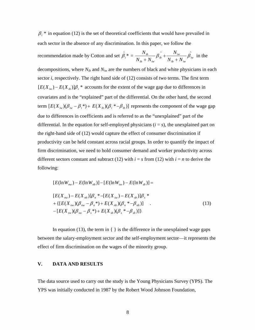
*iβ in equation (12) is the set of theoretical coefficients that would have prevailed in
each sector in the absence of any discrimination. In this paper, we follow the
recommendation made by Cotton and set *∧
iβ = ∧∧
++
+ iwiwib
iwib
iwib
ib
NNN
NNN
ββ in the
decompositions, where Nib and Niw are the numbers of black and white physicians in each
sector i, respectively. The right hand side of (12) consists of two terms. The first term
*)]()([ iibiw XEXE β− accounts for the extent of the wage gap due to differences in
covariates and is the “explained” part of the differential. On the other hand, the second
term +− *))(([ iiwiwXE ββ )]*)(( ibiibXE ββ − represents the component of the wage gap
due to differences in coefficients and is referred to as the “unexplained” part of the
differential. In the equation for self-employed physicians (i = s), the unexplained part on
the right-hand side of (12) would capture the effect of consumer discrimination if
productivity can be held constant across racial groups. In order to quantify the impact of
firm discrimination, we need to hold consumer demand and worker productivity across
different sectors constant and subtract (12) with i = s from (12) with i = n to derive the
following:
=−−− )](ln)(ln[)](ln)(ln[ sbswnbnw WEWEWEWE
)]}*)((*))(([
)]*)((*))(({[*)]()([*)]()([
sbssbsswsw
nbnnbnnwnw
ssbswnnbnw
XEXEXEXE
XEXEXEXE
ββββββββ
ββ
−+−−−+−+
−−−. (13)
In equation (13), the term in { } is the difference in the unexplained wage gaps
between the salary-employment sector and the self-employment sector—it represents the
effect of firm discrimination on the wages of the minority group.
V. DATA AND RESULTS
The data source used to carry out the study is the Young Physicians Survey (YPS). The
YPS was initially conducted in 1987 by the Robert Wood Johnson Foundation,

9
Mathematica Institute, and the American Medical Association to investigate the factors
that influence the career decisions of young physicians (below 40 years of age and had
been in practice for two to six years) and the characteristics of their practices. The survey
contains information on a wide range of variables—such as physician specialty, board
certification status, and waiting time for patients—that would enable us to control for
consumer demand and worker productivity, thereby effectively isolating the effects of
different types of discrimination in the physician market.
There were 5,868 respondents in the original wave of the YPS. Among those
respondents, 3,124 were reinterviewed in 1991 in the second wave of the survey, which
included a total of 6,053 physicians. We first examine the data from the 1987 wave to
detect and decompose any possible discrimination in the market for young physicians.
The group of physicians who were interviewed in both 1987 and 1991 were used to
assess whether the nature of selection into self-employment differs between black and
white physicians.
We restricted the sample used in the estimation to male physicians who worked
for at least 20 hours a week, a minimum of 26 weeks in a year, and who earned a wage
above the federal minimum wage. The final samples include 2,763 white physicians and
396 black physicians from 1987.
Table 1 presents the summary statistics of the variables included in the regression
analysis and table 2 reports employment outcomes associated with physicians in various
demographic and professional categories. In 1987, the number of average weekly work
hours was almost identical for white and black physicians, but blacks had a lower mean
income due to a roughly 11% lower hourly wage ($32.12 vs. $35.60). This wage
differential, however, can be caused by differences in characteristics as the distribution of
specialties varies across races and black physicians are less likely to be married, board
certified, and practice in high income areas.
Among the nine categories of physician specialties listed, blacks have a greater
tendency to specialize in three of them: pediatrics, obstetrics/gynecology, and psychiatry,
which are ranked ninth, fourth, and fifth, respectively, in terms of average hourly
earnings. Thus, based on summary statistics alone, black physicians seem to have a
marginally higher likelihood of being in the less financially lucrative specialties.

10
Consistent with the general findings on the effect of marital status on male earnings,
single male physicians have lower wages and work fewer hours than their married
counterparts. The lower probability of being married also contributes to the lower wages
earned by black physicians. Surprisingly, the status of board certification appears to have
no bearing on one’s wage rate. This unexpected result shows that physicians are not
penalized, at least from the perspective of contemporaneous monetary compensation, for
not being board certified in the beginning stage of their careers. Hence, the substantially
lower rate of board certification among the black physicians in the sample does not
adversely affect their hourly earnings. However, since blacks and whites have almost
identical levels of experience in the sample, the dramatic difference in the rates of board
certification (43.7% vs. 74.2%) suggests that there are perhaps differences in
unobservable determinants of wages between these two groups if the process of obtaining
board certification is not discriminatory against blacks.
The only explanatory variable included in the regression that may lend an
advantage to blacks is the physician-to-population ratio. Black physicians tend to practice
in areas where the physician-to-population ratio is low. This means that black physicians
would, on average, face less competition and their earnings should be higher as a result.
The advantage of less competition enjoyed by black physicians, however, is somewhat, if
not entirely, negated by the lower per capita income of their practice locations.
As established in tables 1 and 2, black physicians, in general, have observable
characteristics that are less favorable to achieving greater earnings. The magnitudes of
these effects on wages are shown in table 3, which entails the estimation results of the
wage regressions used in the Blinder-Oaxaca decompositions. The most striking result
from table 3 is perhaps the size of the experience coefficient for blacks relative to that for
whites.7 At the group mean, wages for black physicians would increase by almost 10.8%
while wages for white physicians would only go up by 8.9%. To the extent of our
knowledge, this is the first study that documents higher returns to experience for blacks
than for whites. We offer three reasons that can help explain this unique result. The first
reason is the homogeneity of the sample used in this study. Most studies of earnings
differentials are based on datasets such as the Current Population Survey and the National
7 The significance of the coefficient on experience for blacks is significant at right around the 10% level.

11
Longitudinal Survey of Youth in which the respondents are drawn from the general
population. If blacks were more likely to be employed in industries where returns to
experience are low, conventional analysis that relies on data compiled from the general
population would underestimate the returns to experience for blacks. The focus on a
single profession in this paper therefore greatly reduces the heterogeneity in earnings due
to the possibility that blacks are concentrated in professions in which returns to
experience are generally low. Second, blacks who choose the career path of physicians
may possess traits that enable them to realize superior returns to experience. Medicine is
one of the most demanding and selective professions. If the environmental factors are less
favorable for blacks to break into the profession, those who eventually succeed in
entering may just have exceptional talents and motivation that are productive
complements of experience. The final explanation is related to psychological factors.
Studies in psychology have found that it is common for whites to hold black physicians
in high esteems. The rationale for this finding is that when two stereotypes (such as the
racial stereotype and the doctor stereotype) are in clash, individuals would only activate
the stereotype that confers them the greatest psychological benefit. Hence, if patients
more often than not have the motivation to suppress any racial stereotypes they have
toward black physicians, it is then more likely for the earnings of black physicians to rise
over time.
The status of being married has a positive effect on wages for white physicians
who are self-employed, but shows no statistically significant effect on physicians in any
other category. Consistent with the summary statistics, board certification has generally
no effect on earnings except in the case of salaried black physicians. Within the subgroup
of salaried black physicians, the achievement of board certification would raise the
hourly wage by about 14%. The coefficients on physician specialties are largely
consistent with the findings in table 2. However, it is worth noting that most of those
coefficients are insignificant for blacks, as there are few blacks in many of the specialty
categories. Finally, the two variables that control for local market conditions (the
physician-to-population ratio and per capita income) have either weak or no effects on
earnings. As the physicians-to-population ratio increase by 10%, i.e., the number of
physicians on a per capita basis decreases by 10%, the hourly wage of self-employed

12
whites would go up by 0.4%, while the hourly wage of salaried blacks would actually
decline by 0.6%. If the per capita income in a local area were to rise by 10%, the hourly
wage of self-employed blacks would increase by 1.6% and the hourly wage of self-
employed whites would go up by about 0.8%.
The details of the Blinder-Oaxaca decompositions are shown in table 4. The
decomposition results suggest that the wage gap among salaried physicians is mostly
attributable to differences in covariates, while the wage differential among self-employed
physicians is entirely due to differences in coefficients. The portion of the wage gap that
can be explained by differences in covariates is actually negative among those who are
self-employed. This means that relative to self-employed white physicians, self-employed
black physicians, on average, have more characteristics associated with higher earnings.
The size of the unexplained self-employed wage gap of .1134 indicates the magnitude of
the black-white wage differential due to consumer discrimination. We can subtract the
unexplained gap of .1134 among the self-employed from the unexplained gap of .0179
among the salaried physicians to quantify the magnitude of the wage differential due to
firm discrimination. The difference in these two gaps is -.0955. Since salaried workers
may suffer from both firm and consumer discrimination, while those who are self-
employed may only be affected by consumer discrimination; the negative difference-in-
differences estimate is quite unexpected. However, we should keep in mind that the
reliability of the estimates derived from the Blinder-Oaxaca decompositions crucially
depends on the conditions of identical demand, equal productivity across employment
sectors within each group, and equal productivity across races within the self-
employment sector being satisfied. We attempt to determine if these conditions hold in
our sample of physicians in the following section.
VI. ROBUSTNESS TESTS
Variations in the Willingness to Pay for Physician Services
Although we control for variables, such as physician-to-population ratios and income per
capita, that can potentially affect the general demand for physicians in each local market,
there may still be a great deal of variations in the demand for physician services within
13
the same local market. Thus, it is important to ensure that the average demand for self-
employed physicians is not significantly different from that for salaried physicians in the
sample. The YPS provides information on the fees charged for office visits and the
number of days a new patient has to wait for an appointment. We use these two variables
to approximate for the demand for each individual physician. Table 5 reports fees
charged for an office visit and waiting time for a new patient depending on whether the
physician owns the practice or is a salaried employee. According to the average waiting
time, salaried physicians seem to have a 40% higher demand than self-employed
physicians. It is worth noting, however, that information on these two variables is missing
for a particularly large number of salaried physicians, as many of them either did not
have knowledge of such information or simply refused to provide it. On the question of
waiting time for an appointment, only 551 out of the 931 salaried physicians who are in
the sample used in regression analysis had a definitive answer (a response rate of 59%),
while 1,095 out of 1,565 possible self-employed physicians gave an exact response (a
rate of 70%). Although there is a much longer waiting time for salaried physicians in the
reduced sample, the fees charged by salaried physicians in the limited sample are only
about 6% higher ($37.74 vs. $35.59) and the difference is not statistically significant. As
pointed out by Reyes (2007), institutional factors, such as health insurance arrangements,
often preclude medical fees from fully adjusting to meet excessive demand. Hence, on
the basis of fees for office visits, the condition of similar willingness to pay for services
provided by self-employed and salaried physicians does not appear to be violated.
While the rigidity of the institutional structure in the healthcare industry may have
brought about similar fees charged by physicians, they do pose a potential problem that
can result in different willingness to pay for physician services depending on whether the
physician is an owner of a practice or just an employee of a healthcare provider. Most
individuals in the United States have health insurance coverage and, hence, do not bear
the full cost of healthcare. Since those individuals who have health insurance only pay a
fraction of the total medical expenses, they would be more likely to pay higher gross
prices for services. Knowing this, self-employed physicians who retain total revenues net
of costs as earnings may purposely seek out clients who have health insurance coverage.
This possibility, once again, can be addressed by the rich data provided by the YPS.
14
There is a question in the YPS asking the respondents to estimate the percentage of
patients in their practices who do not have health insurance coverage. Based on the
responses to this question, we compute the estimated percentage of patients who have
health insurance coverage in each physician’s main practice and present the results in
table 6. As expected, self-employed physicians have a greater proportion of clients with
health insurance coverage then salaried physicians. The difference in percentages,
however, is minimal (91% vs. 87%). The small difference in the proportions of patients
with health insurance coverage between the two groups of physicians is perhaps due to
the inability of salaried physicians to choose their own patients. Instead, it is the owners
of a practice who determine the composition of its clientele and those employers would
also be motivated to pursue patients with health insurance coverage.
The last factor that may lead to systematic variations in the willingness to pay in
the healthcare market pertains to the phenomenon of supplier-induced demand. In certain
market transactions, suppliers have more knowledge about the usefulness and suitability
of the products than demanders and, as a result, demanders rely on suppliers for expert
advice in making the purchase decisions. The providers (physicians) in the healthcare
market, perhaps more so than suppliers in any other markets, dictate the type of services
purchased by the consumers (patients). There is therefore an incentive for physicians to
recommend expensive treatment options and this incentive may be greater for self-
employed than salaried physicians whose earnings are likely to be less dependent on
services provided. Due to data limitation, we cannot directly test whether there is a
difference in the degrees of supplier-induced demand between different types of
physicians. However, past studies have shown that the extent of supplier-induced demand
in the healthcare industry is insignificant.8
Differentials in Productivity
The status as residual claimants for self-employed physicians not only may result in
systematic variations in the consumers’ willingness to pay, as previously noted, it may
also lead to differences in average productivity between self-employed and salaried

15
physicians. It is possible that those physicians who are willing to devote high levels of
effort to work (i.e., physicians who have high productivity conditional on observable
characteristics) would find self-employment particularly attractive since they would be
able to retain residual revenues as earnings. The YPS provides information on the number
of patients seen by a doctor in a week. Combined with the information on the number of
hours physicians spend on patient care per week, we can compute the number of patients
a physician sees on an hourly basis. If self-employed physicians are indeed more
productive than salaried physicians on average, we should perhaps observe a difference
in the number of patients seen per hour between these two groups. Table 7 reports the
average numbers of patients that self-employed and salaried physicians see in an hour.
Surprisingly, it is the salaried physicians who are about 10% more productive overall
(1.91 vs. 1.74 patients per hour). Comparison of physician efficiency is also done for
each individual specialty. However, due to a relatively small number of physicians in
each specialty, the differentials in productivity are all statistically insignificant other than
the case of internal medicine, which happens to be the most popular specialty. Within the
category of internal medicine, salaried physicians are approximately 18% more efficient
in producing office visits (1.72 vs. 1.46 patients per hour).9
The number of patient visits per hour by employment sector and race are
presented in table 8. The group difference in productivity between black and white
physicians is not statistically significant and that suggests the estimate of the effect of
consumer discrimination is perhaps reliable despite a much lower rate of board
certification among black physicians. Among both blacks and whites, salaried physicians
see more patients per hour than self-employed physicians; salaried black physicians
8 Rossiter and Wilensky (1984) find that a 10% increase in physician density would raise both utilization and expenditures on physician services by approximately 1%. Stano (1987) argues that the magnitude of the elasticity is even smaller than that. 9 There is a note of caution in equating the number of office visits a physician generates to how efficient that physician is. As recognized by Langwell (1982), when the number of patient visits in a given time interval is used to proxy for physician efficiency, average quality of the service provided is implicitly assumed to be constant, but that assumption may not be correct in reality. It is possible that self-employed physicians are more inclined to provide a higher average quality office visit by spending more time with each patient as a way of generating repeat customers. Salaried physicians, on the other hand, may have more of an incentive to get patients quickly out of their offices in order to leave work at a reasonable hour. Hence, the greater number of office visits produced in an hour by salaried physicians does not necessarily imply higher productivity.
16
produce 14% more patient visits than self-employed black physicians, while salaried
white physicians generate almost 7% more patient visits than self-employed white
physicians, and both differentials are statistically significant. The statistically significant
productivity differential within each group seems to have violated one of the (sufficient)
conditions for the clear-cut interpretation of the double difference in wage gaps. The
larger productivity differential among blacks is consistent with a negative self-selection
into self-employment by blacks (relative to whites), as documented by Borjas and
Bronars (1989) and Kawaguchi (2005). If black physicians negatively self-select into
self-employment relative to white physicians, the double difference in wage gaps would
understate the effect of firm discrimination, as can be clearly seen from equation (9).
We exploit the longitudinal element of the YPS to further investigate the issue of
negative selection into self-employment among black physicians. After applying various
sample restrictions, there are 1,470 black or white male physicians who have valid
employment and wage data in both the 1987 and 1991 surveys. Table 9 tabulates their
employment transitions from 1987 to 1991. The number of physicians who changed their
employment sectors from 1987 to 1991 is relatively small. There were a total of 248
physicians who switched from the salary-employment sector to the self-employment
sector, while 96 physicians made the reverse move. The number of blacks who moved
from one employment sector to the other is even smaller—only 42 of them made the
switch either way.
In order to determine if the nature of selection into self-employment is indeed
different between black and white physicians, we compare the 1987 wages of those who
switched sectors between 1987 and 1991 with the 1987 wages of those who remained in
the same sectors within each racial group. Those comparisons are reported in table 10.
Among blacks who were employees of healthcare providers in 1987, those who switched
to self-employment in 1991 had a 5% lower average wage in 1987 than those who
remained as employees. The difference of 5%, however, is not statistically significant.
Among whites who were salaried physicians in 1987, the ones who moved to the self-
employment sector had a 7% higher wage in 1987 than the ones who did not make the
move. Among the physicians who were self-employed in 1987, no statistically significant
relationships can be found between the average wage of sector switchers and that of
17
nonswitchers within either blacks or whites. Considering all the evidence, black
physicians seem to exhibit a negative selection into self-employment relative to white
physicians.
VII. CONCLUSION
A difference-in-differences strategy is proposed in this paper to decompose the
contributions of different types of discrimination to the black-white wage differential.
The strategy is based on the intuition that self-employed individuals are not likely to be
subject to firm discrimination, while salaried workers may suffer from both firm and
consumer discrimination. Hence, after controlling for all the characteristics that can
potentially affect earnings, the wage difference between self-employed black and white
workers can be attributed to consumer discrimination, while the wage difference between
salaried black and white workers in excess of the difference between self-employed black
and white workers is attributable to firm discrimination.
The sufficient conditions under which the difference and double difference
estimates would accurately reflect the distinct effects of consumer and firm
discrimination on earnings are derived in a general framework. In order for the wage
difference between self-employed black and white workers to correctly measure the
effect of consumer discrimination, these two groups of workers must be equally
productive. The difference-in-differences estimate would precisely indicate the fraction
of the racial wage gap that results from firm discrimination if consumer’s willingness to
pay is identical for both self-employed and salaried workers, and if self-employed and
salaried workers are equally productive within each racial group.
Data from the Young Physicians Survey is used to implement the proposed
strategy. The results suggest that potential discrimination plays a small role in the racial
wage gap among physicians. At most, discrimination lowers the hourly wages of black
physicians by 3.3%. The decompositions show that consumer discrimination accounts for
all of the potential discrimination in the physician market and that the effect of firm
discrimination is actually in favor of black physicians. The interpretations of the
estimates, however, are complicated by the possibility that relative to white physicians,

18
black physicians negatively self-select into self-employment. This relative negative
selection into self-employment by blacks would both overestimate the effect of consumer
discrimination and underestimate the effect of firm discrimination.
19
REFERENCES
Aigner, Dennis J., and Glen C. Cain. 1977. “Statistical Theories of Discrimination in the Labor Market.” Industrial and Labor Relations Review 30(2): 175–87.
Arrow, Kenneth J. 1973. “The Theory of Discrimination.” in Orley Ashenfelter and
Albert Rees (eds.), Discrimination in the Labor Market. Princeton, NJ: Princeton University Press.
Becker, Gary. 1957. The Economics of Discrimination. Chicago: University of Chicago
Press. Blinder, Alan S. 1973. “Wage Discrimination: Reduced Form and Structural Estimates.”
The Journal of Human Resources 8(4): 436–455. Borjas, George J., and Stephen G. Bronars. 1989. “Consumer Discrimination of Self-
Employment.” Journal of Political Economy 97(3): 581–605. Cain, Glen C. 1986. “The Economic Analysis of Labor Market Discrimination: A
Survey.” in Orley Ashenfelter and Richard Layard(eds.), Handbook of Labor Economics, Volume 1. Amsterdam: North-Holland.
Cotton, Jeremiah. 1988. “On the Decomposition of Wage Differentials.” The Review of
Economics and Statistics 70(2): 236–243. Holzer, Harry J., and Keith R. Ihlanfeldt. 1998. “Customer Discrimination and
Employment Outcomes for Minority Workers.” Quarter Journal of Economics 113(3): 835–867.
Jann, Ben. 2008. “A STATA Implementation of the Blinder-Oaxaca Decomposition.”
Working Paper No. 5. Zurich: Eidgenössische Technische Hochschule (ETH). Kawaguchi, Daiji. 2005. “Negative Self-Selection into Self-employment among African
Americans.” Topics in Economic Analysis and Policy 5(1): 1356. Kunda, Ziva, and Lisa Sinclair. 1999a. “Motivated Reasoning with Stereotypes:
Activation, Application, and Inhibition.” Psychological Inquiry 10(1): 12–22. ————. 1999b. “Reactions to a Black Professional: Motivated Inhibition and
Activation of Conflicting Stereotypes.” Journal of Personality and Social Psychology 77(5): 885–904.
Langwell, Karen. 1982. “Factors Affecting the Incomes of Men and Women Physicians:
Further Explanations.” The Journal of Human Resources 17(2): 261–275.
20
Lundberg, Shelly J., and Richard Startz. 1983. “Private Discrimination and Social Intervention in Competitive Labor Markets.” American Economic Review 73(3): 340–347.
Nardinelli, Clark, and Curtis Simon. 1990. “Customer Racial Discrimination in the
Market for Memorabilia: The Case of Baseball.” Quarterly Journal of Economics 105(3): 575–595.
Oaxaca, Ronald. 1973. “Male-Female Wage Differentials in Urban Labor Markets.”
International Economic Review 14(3): 693–709. Oaxaca, Ronald, and Michael R. Ransom. 1994. “On Discrimination and the
Decomposition of Wage Differentials.” Journal of Econometrics 61(1): 5–21. O’Neill, June E., and Dave M. O’Neill. 2005. “What Do Wage Differentials Tell Us
about Labor Market Discrimination?” Working Paper No. 11240. Cambridge, MA: National Bureau of Economic Research (NBER).
Oettinger, Gerald S. 1996. “Statistical Discrimination and the Early Career Evolution of
the Black-White Wage Gap.” Journal of Labor Economics 14(1): 52–78. Reimers, Cordelia W. 1983. “Labor Market Discrimination against Hispanic and Black
Men.” The Review of Economics and Statistics 65(4): 570–579. Reyes, Jessica Wolpaw. 2007. “Reaching Equilibrium in the Market for Obstetricians and
Gynecologists.” American Economic Review 97(2): 407–411. Rossiter, Louis F., and Gail R. Wilensky. 1984. “Identification of Physician-Induced
Demand.” Journal of Human Resources 19(2): 231–244. Rosen, Asa. 2003. “Search, Bargaining, and Employer Discrimination.” Journal of Labor
Economics 21(4): 807–829. Sasaki, Masaru. 1999. “An Equilibrium Search Model with Co-workers Discrimination.” Journal of Labor Economics 17(2): 377–407. Sasser, Alicia C. 2004. “Gender Differences in Physician Pay: Tradeoffs between Career
and Family.” Journal of Human Resources 40(2): 477–504. Stano, Miron. 1987. “A Clarification of Theories and Evidence on Supplier-Induced
Demand for Physicians’ Services.” Journal of Human Resources 22(4): 611–620. Yun, Myeong-Su. 2005. “A Simple Solution to the Identification Problem in Detailed
Wage Decompositions.” Economic Inquiry 43(4): 766–772.

21
TABLES
Table 1. Summary Statistics Blacks Whites Hourly Wage 34.9 (27.59) 37.53 (27.44)Weekly Hours* 60.64 (19.05) 60.75 (14.83)Annual Income* 93,930 (57,840) 103,800 (72,170)Married .745 (.437) .858 (.349)Years of Experience 3.521 (1.129) 3.477 (1.152)Board Certified .45 (.498) .744 (.436)Physician Specialty: General Practice .135 (.342) .18 (.384) Internal Medicine .238 (.426) .256 (.436) Surgery .202 (.402) .213 (.409) Pediatrics .099 (.3) .063 (.243) Obgyn .128 (.334) .049 (.215) Radiology .025 (.156) .051 (.22) Psychiatry .053 (.225) .043 (.204) Anesthesiology .043 (.202) .053 (.224) Other Specialties .078 (.269) .093 (.291)Physican-to-population ratio 505.1 (872.1) 552.6 (862.4)Per capita income 11,426 (5,397) 12,647 (4,935)Number of physicians 282 2,214 Notes: 1. * indicates that the variable is not included in the regression analysis. 2. The numbers in ( ) indicate standard errors.
Table 2. Employment Outcomes in Each Category in 1987 Hourly Wage Weekly Hours Annual Income Married 37.54 60.98 104,013 Nonmarried 35.55 59.40 95,664 Board certified 37.18 60.67 102,889 Non-board certified 37.36 60.90 102,300 Specialties: General Practice 26.97 59.25 73,560 Internal Medicine 30.46 61.91 87,548 Surgery 48.45 64.32 140,646 Pediatrics 26.16 59.65 71,725 Obgyn 40.31 67.24 121,139 Radiology 48.54 54.25 115,492 Psychiatry 38.67 53.30 92,586 Anesthesiology 55.95 60.67 145,651 Other Specialties 38.57 55.78 97,750

22
Table 3. Wage Equation Estimates for the Year 1987
All Physicians Self-Employed Salaried Blacks Whites Blacks Whites Blacks Whites
Intercept 1.6111 (.8305)
2.3820 (.3206)
2.4424 (1.2440)
2.7621 (.4553)
1.1211 (.9002)
2.5475 (.4160)
Married -.00876 (.0775)
.0796 (.0306)
-.0416 (.1285)
.1004 (.0434)
.0454 (.0743)
.0241 (.0394)
Experience .3070 (.1867)
.2535 (.0632)
.2156 (.3041)
.3377 (.0876)
.4754 (.1856)
.0291 (.0854)
Experience2 -.0287 (.0257)
-.0239 (.0088)
-.0161 (.0410)
-.0346 (.0120)
-.0531 (.0260)
.0033 (.0121)
Board .1109 (.0726)
.0101 (.0260)
.1150 (.1147)
-.0074 (.0345)
.1432 (.0732)
.0382 (.0366)
General practice -.2445 (.0956)
-.3410 (.0276)
-.3437 (.1477)
-.3954 (.0357)
-.0894 (.0867)
-.2069 (.0411)
Internal medicine -.2200 (.0736)
-.2063 (.0229)
-.2757 (.1189)
-.2099 (.0310)
-.1323 (.0709)
-.1978 (.0317)
Surgery .1472 (.0785)
.1928 (.0241)
.1415 (.1143)
.1765 (.0307)
.0765 (.0898)
.1371 (.0389)
Pediatrics -.1644 (.1025)
-.3581 (.0396)
-.2436 (.1751)
-.3927 (.0594)
-.0249 (.0918)
-.2814 (.0479)
Obgyn .2884 (.0926)
-.0412 (.0447)
.3534 (.1404)
-.0199 (.0574)
.2451 (.0992)
-.1388 (.0667)
Radiology .2249 (.1926)
.2906 (.0437)
.4257 (.3036)
.3356 (.0634)
-.0629 (.1880)
.2603 (.0544)
Psychiatry .1198 (.1353)
-.0348 (.0471)
.2416 (.2712)
-.093 (.0616)
.1663 (.1114)
.0669 (.0679)
Anesthesiology -.03320 (.1495)
.4357 (.0430)
-.1301 (.1831)
.4747 (.0553)
-.0894 (.0867)
.2711 (.0647)
Other specialties -.1181 (.1134)
.0624 (.0334)
-.1691 (.1742)
.1242 (.0537)
-.0889 (.1149)
.0896 (.0385)
Ln (md-pop ratio) -.0009 (.0291)
-.0036 (.0098)
.0668 (.0458)
.0401 (.0143)
-.0670 (.0302)
-.0126 (.0128)
Ln (per capita income) .1145 (.0859)
.0551 (.0325)
.0124 (.1325)
-.0206 (.0469)
.1615 (.0905)
.0777 (.0414)
Ln (wage) 3.3647 3.4590 3.4300 3.5315 3.2697 3.3348 R2 .1560 .2173 .1759 .2484 .2665 .1736 N 282 2214 167 1398 115 816 Notes: 1. The dependent variable is the natural log of the hourly wage. 2. The numbers in ( ) indicate standard errors. 3. Following Yun (2005), we estimate the “normalized” wage regressions. Hence, the coefficient on each
physician specialty expresses the wage deviation in percentages from the mean of all specialties.

23
Table 4. The Blinder-Oaxaca Decompositions All physicians Self-employed Salaried Total wage gap .0944 .1015 .0651 Explained wage gap .0243 -.0119 .0473 Unexplained wage gap .0701 .1134 .0179 Note: Difference in unexplained wage gaps between self-employed and salaried physicians = -.0955
Table 5. Fees and Waiting Time (in Days) for Appointment Self-employed physicians Salaried physicians Differential
Fees charged $35.59 (22.57)
N = 1,275
$37.74 (32.18) N = 406
-$2.15 (1.72)
Waiting time 8.39
(16.59) N = 1,095
11.73 (15.23) N = 551
-3.34 (.82)
Note: The numbers in ( ) indicate standard errors.
Table 6. Proportion of Patients with Insurance Self-employed physicians Salaried physicians Differential
.9071 (.1012)
N = 1,465
.8713 (.1598) N = 684
.0359 (.0067)
Note: The numbers in ( ) indicate standard errors.

24
Table 7. Number of Patients Seen in an Hour by Specialty and Employment Sector Self-employed Physicians Salaried
physicians Differential
All Specialties 1.7364
(1.0355) N = 1,309
1.9084 (1.4865) N = 777
-0.172 (0.0605)
General Practice 2.2242
(1.0015) N = 289
2.3478 (1.2323) N = 142
-.1236 (.1190)
Internal Medicine
1.4605 (.85)
N = 379
1.7221 (1.5225) N = 240
-.2616 (.1075)
Surgery 1.5755 (.9333) N = 315
1.6822 (1.3503) N = 121
-.1067 (.1335)
Pediatrics 2.1153
(1.0222) N = 79
1.9455 (1.44) N = 85
.1698 (.1940)
Obgyn 1.49
(.6303) N = 94
1.5765 (.9669) N = 49
-.0865 (.1527)
Radiology 5.5
(1.8028) N = 3
3.348 (3.4234)
N = 5
2.152 (1.8513)
Psychiatry .9548
(.5179) N = 66
.9414 (.6927) N = 42
.0134 (.1245)
Anesthesiology .7018
( ) N = 1
2.9444 (2.907) N = 2
-2.2426 (2.0556)
Other Specialties 2.3247
(1.5192) N = 83
2.503 (1.833) N = 91
-.1783 (.2544)
Note: The numbers in ( ) indicate standard errors.

25
Table 8. Number of Patients Seen in an Hour by Race and Employment Sector Blacks Whites Differential
All 1.7303
(1.0621) N = 246
1.8098 (1.2458)
N = 1,840
-.0795 (.0737)
Self-employed 1.6243 (.8884)
N = 140
1.7498 (1.0513)
N = 1,169
-.1255 (.0811)
Salaried 1.8704
(1.2461) N = 106
1.9144 (1.5217)
N = 671
-.044 (.1249)
Differential -.2461 (.1424)
-.1646 (.0663)
Note: The numbers in ( ) indicate standard error.
Table 9. Employment Transition from 1987 to 1991 Salaried employee
in 1991 Self-employed in 1991
Salaried employee in 1987 N = 499
Blacks = 75 Whites = 424
N = 248 Blacks = 25
Whites = 223
Self-employed in 1987 N = 96
Blacks = 17 Whites = 79
N = 627 Blacks = 71
Whites = 556
Table 10. Wage (from 1987) Comparisons between Sector Switchers and Non-sector Switchers
Blacks Whites Salaried
employee in 1991
Self- employedin 1991
DifferentialSalaried employeein 1991
Self- employed in 1991
Differential
Salaried employee in 1987
26.7 (10.03) N = 75
25.48 (12.62) N = 25
-1.22 (3.52)
28.41 (12.03) N = 424
30.4 (15.03) N = 223
1.99 (1.16)
Self-employed in 1987
36.81 (25.59) N = 17
34.98 (24.72) N = 71
-1.83 (6.86)
39.66 (26.58) N = 79
39.34 (24.82) N = 556
-.32 (3.17)
Note: The numbers in ( ) indicate standard errors.


