Decomposition of Atmospheric Disturbances into Standing and Traveling Components,with Application to Northern Hemisphere Planetary Waves and
Stratosphere–Troposphere Coupling
OLIVER WATT-MEYER AND PAUL J. KUSHNER
Department of Physics, University of Toronto, Toronto, Ontario, Canada
(Manuscript received 22 July 2014, in final form 26 September 2014)
ABSTRACT
This study updates a body of literature that aims to separate atmospheric disturbances into standing and
traveling zonal wave components. Classical wavenumber–frequency analysis decomposes longitude- and
time-dependent signals into contributions from distinct spatial and temporal scales. Here, an additional de-
composition of the spectrum into standing and traveling components is described. Previous methods de-
compose the power spectrum into standing and traveling parts with no explicit allowance for covariance
between the two. This study provides a simple method to calculate the variance of each of these components
and the covariance between them. It is shown that this covariance is typically a significant portion of the
variance of the total signal. The approach also preserves phase information and allows for the reconstruction
of the real-space standing and traveling components.
The technique is applied to reanalysis wintertime geopotential height anomalies in the Northern Hemi-
sphere in order to investigate planetary wave interference effects in stratosphere–troposphere coupling. The
results show that for planetary waves 1–3, standing waves explain the largest portion of the variance at low
frequencies. An exception is for wave 1 in the high-latitude troposphere, where there is a strong westward-
traveling wave. Furthermore, the antinodes of the standing waves have preferred longitudes that tend to align
with the extremes of the climatological wave, suggesting that standing waves contribute to a linear in-
terference effect that has been shown to be an important part of stratosphere–troposphere interactions.
1. Introduction
Wavenumber–frequency spectral analysis is often
used to decompose large-scale atmospheric flows into
spatial and temporal Fourier harmonics (e.g., Hayashi
1971;Wheeler andKiladis 1999), which can then be used
to compute cross-spectra for quantities such as meridi-
onal heat or momentum flux (Randel and Held 1991).
Here we consider the problem of further decomposing
each Fourier harmonic into standing and traveling
components. In this work a standing wave is defined to
be like a standing wave on a string with fixed ends—that
is, of the form cos(kl) cos(vt). It is the sum of two op-
positely traveling waves of equal amplitude and phase
speed: 2cos (kl) cos(vt)5 cos(kl2 vt)1 cos(kl1 vt).
Note that in some studies, ‘‘standing wave’’ is used to
refer to the climatological zonal asymmetry; we will
refer to this latter quantity simply as the climatological
wave. Estimation of standing and traveling wave power
spectra has been described previously (Hayashi 1973,
1977, 1979; Pratt 1976). However, themethods proposed
by Hayashi and Pratt both suffer from the same issue:
they exclusively decompose the power spectrum into
standing and traveling parts with no possibility for any
covariance between these wave structures. We will show
that although such decompositions are not unique, typ-
ical prescriptions yield standing waves that are not
orthogonal to the traveling waves and hence include
significant covariance.
In this report, we propose a simple decomposition of
the wavenumber–frequency spectrum into standing and
traveling parts, calculate analytic expressions for the
variance of each component and their covariance, and
show how the decomposition can be used to reconstruct
standing and traveling wave fields. While the techniques
that we describe are quite general, we were motivated to
carry out this analysis by particular issues related to
Corresponding author address:Oliver Watt-Meyer, Department
of Physics, University of Toronto, 60 St. George St., Toronto ON
M5S 1A7, Canada.
E-mail: [email protected]
FEBRUARY 2015 WATT -MEYER AND KUSHNER 787
DOI: 10.1175/JAS-D-14-0214.1
� 2015 American Meteorological Society

wave-driven stratosphere–troposphere coupling in the
Northern Hemisphere extratropics (Baldwin and
Dunkerton 2001; Garfinkel et al. 2010; Shaw et al. 2010;
Smith and Kushner 2012). Thus, we apply the tech-
nique to geopotential height anomalies in the Northern
Hemisphere winter. Example case studies of interest
are shown in Fig. 1. In the left column in Fig. 1 we show
Hovmöller plots of the wave-1 geopotential heightanomalies at 608N and 100hPa for the winter of 1979/80,
which consisted of persistent westward-propagatingwave-1
anomalies, and for the winter of 1990/91, which was dom-
inated by a large-amplitude standing wave event. Our in-
terest is in how these different wave anomalies interfere
with the background climatology and, thus, drive fluctua-
tions in the portion of the vertical flux of wave activity—as
measured by themeridional eddy heat flux—that is linearly
coherent with the background climatological wave (Nishii
et al. 2009). We denote this quantity ‘‘LIN’’ (Smith and
Kushner 2012). The second column in Fig. 1 shows the
wave-1 component of LIN for each of these winter sea-
sons. The positive and negative periods of LIN corre-
spond towave-1 anomalies being, respectively, in and out
of phase with the wave-1 background climatology (the
longitudes of the maximum and minimum of the daily
wave-1 climatology are indicated by the solid and dashed
black lines). A standing–traveling decomposition will
allow us to determine whether fluctuations in LIN are
being driven primarily by traveling waves of consistent
amplitude propagating in and out of phase with the
background or by standing waves fixed in space.
Computations of standing and traveling wave de-
compositions of the extratropical circulation have to
FIG. 1. Wave-1 Z*0 and LIN heat flux at 608N and 100 hPa for two NDJFM seasons: (top) 1979/80 and (bottom)
1990/91. (left)–(right) Wave-1 Z*0, wave-1 component of LIN heat flux, wave-1 Z*0St, and wave-1 Z*0
Tr. The contour
levels for all the Hovmöller diagrams are 6(0, 100, 200, 300, 400, 500)m, where the reds are positive and blues are
negative. The solid and dashed black lines on the farthest left panels show the daily position of the maximum and
minimum of the wave 1 of Zc*. Note that for each row the two right panels sum to the leftmost panel.
788 JOURNAL OF THE ATMOSPHER IC SC IENCES VOLUME 72
a large extent relied on the methods of Hayashi (1977,
1979) and Pratt (1976). These methods were summa-
rized in the textbook by von Storch and Zwiers (1999).
For example, Fraedrich and Böttger (1978) decompose
the spectrum of geopotential heights at 500 hPa and
508N into standing and traveling parts using a method
that combines the techniques of Pratt and Hayashi.
Their focus is on higher wavenumber and frequency
disturbances, where the authors observe several distinct
peaks in the spectrum. The authors suggest that differing
types of baroclinic instability—associated with dry ver-
sus moist static stability—could be responsible for these
separate peaks. Speth and Madden (1983), using the
Hayashi (1977) method, highlight and investigate in
more detail the presence of a high-latitude 15–30-day
period westward-traveling wave-1 feature. Using the
meridional and vertical structure of the feature’s am-
plitude as evidence, the authors attribute it to a mani-
festation of the theoretically predicted 16-day wave
(Haurwitz 1940; Madden 1979). Other studies have used
Hayashi and Pratt’s methods to determine whether the
Madden–Julian oscillation is primarily a standing or prop-
agating pattern (Zhang and Hendon 1997); to analyze the
atmospheric variability in general circulation models
and its dependence on the El Niño–SouthernOscillation
(May 1999); and to quantify midlatitude tropospheric
variability, and possible changes to it under global warm-
ing scenarios, in the Coupled Model Intercomparison
Project phase 3 (Lucarini et al. 2007) and phase 5 (Di
Biagio et al. 2014) ensembles.
These examples show the potentially wide applica-
bility of standing–traveling wave decompositions. We
will show that the previously used decomposition
methods, however, do not explicitly account for the lack
of uniqueness of these decompositions or for the non-
orthogonality of the resulting wave fields. These short-
comings and their implications will be addressed in this
report, which is structured as follows. Section 2 will
outline the proposed standing–traveling decomposition,
describe some simple analytical results, outline pre-
viously defined techniques, and describe the data to
which we apply the analysis technique. Section 3 will
show the results of applying the method to Northern
Hemisphere geopotential height anomalies, including
a detailed comparison with previous approaches and an
overview of the climatological wavenumber–frequency
spectra in the extratropics. To investigate planetary
wave interference effects, we will compare the structure
of the standing waves and the climatological wave field.
Last, we will compute the vertical and time-lagged co-
herences of the standing and traveling waves at selected
Northern Hemisphere extratropical locations using
correlation-coherence analysis (Randel 1987). Section 4
will summarize the results and discuss implications for
stratosphere–troposphere coupling.
2. Theory and data
a. Standing–traveling wave decomposition
This section describes our proposed decomposition of
the wavenumber–frequency spectrum into standing and
traveling parts. To begin, given some longitude- and
time-dependent variable q(l, t), with daily frequency
over a period of time of length T days and defined at N
equally spaced points in longitude, the discrete 2D
Fourier transform is computed as
qk,j 5 �N21
n50�T21
t50
e2ikln2iv
jtq(ln, t) , (1)
where ln 5 2pn/N andvj 5 2pj/T, defined for k5 0, . . . ,
N 2 1 (k is the planetary wavenumber) and j 5 0, . . . ,
T 2 1 ( j is an integer index that corresponds to the
frequency vj). For simplicity, q(l, t) is assumed to have
zero zonal and time means, and N and T are assumed to
be odd. Given that q(l, t) is real, as shown in the ap-
pendix, one can write the inverse transform as
q(l, t)52
NT�N
2
k51�T
2
j51
qk,6j(l, t) , (2)
where N2 5 (N 2 1)/2, T2 5 (T 2 1)/2, and
qk,6j(l, t)5Qk,j cos(kl1vjt1fk,j)
1Qk,2j cos(kl2vjt1fk,2j) , (3)
where we have used v2j 5 2vj and where Qk,j and fk,j
are the amplitude and phase of qk,j. That is, qk,j 5Qk,jeifk,j ,
with Qk,j real and positive and 2p , fk,j # p.
We now decompose the amplitudes Qk,j in Eq. (3) in
order to express q(l, t) as a combination of standing and
traveling waves at each wavenumber and frequency.
Using the fact that a pure standing wave consists of two
traveling waves of equal amplitude and phase speed
moving in opposite directions, we define standing and
traveling amplitudes as
QStk,j 5min(Qk,j,Qk,2j) and (4a)
QTrk,j 5Qk,j 2QSt
k,j (4b)
and note that these definitions imply that QStk,j 5QSt
k,2j
and that either QTrk,j 5 0 or QTr
k,2j 5 0. Furthermore, we
note that QStk,j and QTr
k,j are real and nonnegative. The
FEBRUARY 2015 WATT -MEYER AND KUSHNER 789
phases of the standing and traveling components are set
to be equal to the original Fourier coefficient phases;
that is, fStk,j 5fTr
k,j 5fk,j. A phasor representation in the
complex plane of this decomposition of two Fourier co-
efficients qk,6j into standing and traveling components is
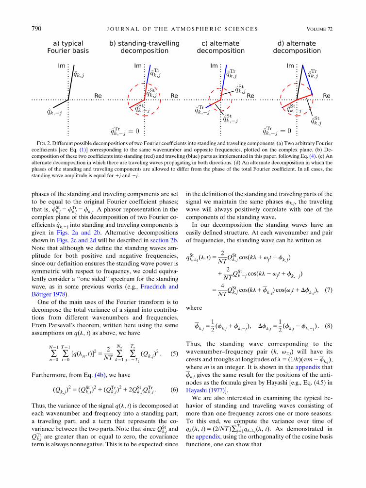
given in Figs. 2a and 2b. Alternative decompositions
shown in Figs. 2c and 2d will be described in section 2b.
Note that although we define the standing waves am-
plitude for both positive and negative frequencies,
since our definition ensures the standing wave power is
symmetric with respect to frequency, we could equiva-
lently consider a ‘‘one sided’’ spectrum for the standing
wave, as in some previous works (e.g., Fraedrich and
Böttger 1978).One of the main uses of the Fourier transform is to
decompose the total variance of a signal into contribu-
tions from different wavenumbers and frequencies.
From Parseval’s theorem, written here using the same
assumptions on q(l, t) as above, we have
�N21
n50�T21
t50
[q(ln, t)]25
2
NT�N
2
k51�T2
j52T2
(Qk, j)2 . (5)
Furthermore, from Eq. (4b), we have
(Qk, j)2 5 (QSt
k, j)21 (QTr
k, j)21 2QSt
k, jQTrk, j . (6)
Thus, the variance of the signal q(l, t) is decomposed at
each wavenumber and frequency into a standing part,
a traveling part, and a term that represents the co-
variance between the two parts. Note that sinceQStk,j and
QTrk,j are greater than or equal to zero, the covariance
term is always nonnegative. This is to be expected: since
in the definition of the standing and traveling parts of the
signal we maintain the same phases fk,j, the traveling
wave will always positively correlate with one of the
components of the standing wave.
In our decomposition the standing waves have an
easily defined structure. At each wavenumber and pair
of frequencies, the standing wave can be written as
qStk,6j(l, t)52
NTQSt
k, j cos(kl1vjt1fk, j)
12
NTQSt
k,2j cos(kl2vjt1fk,2j)
54
NTQSt
k, j cos(kl1fk, j) cos(vjt1Dfk, j), (7)
where
fk,j51
2(fk,j 1fk,2j), Dfk,j 5
1
2(fk,j 2fk,2j) . (8)
Thus, the standing wave corresponding to the
wavenumber–frequency pair (k, v6j) will have its
crests and troughs at longitudes of l5 (1/k)(pm2fk,j),
where m is an integer. It is shown in the appendix that
fk,j gives the same result for the positions of the anti-
nodes as the formula given by Hayashi [e.g., Eq. (4.5) in
Hayashi (1977)].
We are also interested in examining the typical be-
havior of standing and traveling waves consisting of
more than one frequency across one or more seasons.
To this end, we compute the variance over time of
qk(l, t)5 (2/NT)�T2
j51qk,6j(l, t). As demonstrated in
the appendix, using the orthogonality of the cosine basis
functions, one can show that
FIG. 2. Different possible decompositions of two Fourier coefficients into standing and traveling components. (a) Two arbitrary Fourier
coefficients [see Eq. (1)] corresponding to the same wavenumber and opposite frequencies, plotted on the complex plane. (b) De-
composition of these two coefficients into standing (red) and traveling (blue) parts as implemented in this paper, following Eq. (4). (c) An
alternate decomposition in which there are traveling waves propagating in both directions. (d) An alternate decomposition in which the
phases of the standing and traveling components are allowed to differ from the phase of the total Fourier coefficient. In all cases, the
standing wave amplitude is equal for 1j and 2j.
790 JOURNAL OF THE ATMOSPHER IC SC IENCES VOLUME 72

var(qk)(l)51
T�T21
t50
[qk(l, t)]2
52
N2T2 �T
2
j52T2
[Q2k,j 1 2Qk,jQk,2j cos
2(kl1fk,j)2Qk,jQk,2j] , (9)
where fk,j was defined in Eq. (8). If the signal qk(l, t) is
the sum of pure standing waves (i.e., Qk,j 5 Qk,2j) then
Eq. (9) simplifies to
var(qStk )(l)54
N2T2 �T2
j52T2
Q2k, j cos
2(kl1fk, j) . (10)
On the other hand, if our signal is the sum of pure trav-
eling waves (i.e., either Qk,j 5 0 or Qk,2j 5 0 for every j;
i.e., Qk,jQk,2j 5 0), then Eq. (9) simplifies to
var(qTrk )(l)52
N2T2 �T2
j52T2
Q2k, j . (11)
b. Alternate decompositions
Because the standing and traveling waves at the same
wavenumber and frequency are not orthogonal, the de-
composition defined inEq. (4) is not unique. For example,
one could assign less amplitude to the standing wave and
have traveling waves moving in both directions at each
absolute frequency, as in Hayashi (1977). An example of
this is shown in Fig. 2c. Furthermore, if one allows for the
phases of the standing and traveling components to be
different, then this allows another set of possibilities for
the decomposition, an example of which is shown in
Fig. 2d. Nevertheless, we argue that our choice defined
in Eq. (4) is a natural decomposition to work with for
a number of reasons. First, we reject the possibility of
having traveling waves moving in both directions at the
same wavenumber and phase speed, as in Fig. 2c, since
these will just add up to an additional standing wave at
this frequency. Second, we choose to keep the same
phases for the standing and traveling components, be-
cause this is the simplest choice and because it ensures
that the standing and traveling parts of the signal each
have the maximum correlation with the total signal.
Note that if we allow the phases of the standing and
traveling components to vary, as in Fig. 2d, the covariance
can also be negative or zero. In particular, assuming only
that qk,j 5 qStk,j 1 qTrk,j, we can generalize Eq. (6) to
(Qk, j)25 (QSt
k, j)21 (QTr
k, j)21 2QSt
k, jQTrk, j cos(f
Stk, j 2fTr
k, j) .
(12)
When fStk,j 5fTr
k,j as before, we recover Eq. (6) and the
covariance is strictly positive. However, it is also possible to
forcefStk,j 2fTr
k,j 5 6p/2 (one of these cases is illustrated in
Fig. 2d) in which case the covariance will be zero. Never-
theless, the fStk,j 5fTr
k,j case is the most intuitive de-
composition because it maximizes the correlation between
eachof the standing and traveling components and the total
signal. This follows from the fact that the Fourier co-
efficients for the standing and traveling waves are parallel
to the total coefficient in the complex plane (as in Fig. 2b).
As far as we are aware, all standing–traveling de-
compositions discussed in the literature (Hayashi 1973,
1977, 1979; Pratt 1976) do not explicitly account for the
covariance term between standing and traveling waves.
The authors generally take it as an assumption that the
standing and traveling waves will be independent, al-
though they do recognize that this is not always actually
the case. In particular, they require that, written in our
notation, either (Qk,j)2 5 (QSt
k,j)2 1 (QTr
k,j)2 1 noise (Pratt
1976) or (Qk,j)2 5 (QSt
k,j)2 1 (QTr
k,j)2 (Hayashi 1977) with-
out any explicit representation of covariance between the
standing and traveling parts of the signal.
We thus identify two distinct advances arising from our
technique. First, we can precisely account for and calcu-
late the often significant contribution from the joint var-
iability of standing and traveling waves. Second, it is also
straightforward to reconstruct the real-space standing
and traveling parts of the signal,1 which is something that
is not simple to do with the other techniques.
c. Other techniques
Some previous techniques for computing the
wavenumber–frequency spectrum, starting with Hayashi
(1971), take a somewhat different approach thanwhat we
have described above. They begin by computing a spatial
Fourier transform of q(l, t) at each time step and defining
ck(t) and sk(t) as the time series for the cosine and sine
coefficients at wavenumber k (again, we are assuming the
zonal mean of q is zero):
q(l, t)5 �N
k51
[ck(t) cos(kl)1 sk(t) sin(kl)] . (13)
1To do this, simply use the inverse transform given in Eqs. (2)
and (3) with the standing or traveling amplitudes, QStk,j or Q
Trk,j, in-
stead of the total amplitude Qk,j.
FEBRUARY 2015 WATT -MEYER AND KUSHNER 791
The wavenumber–frequency spectrum is then defined as
[see also von Storch and Zwiers (1999)]
Pk,v(q)5Pv(ck)1Pv(sk)
21Qv(ck, sk) , (14)
where Pv(ck) and Pv(sk) are the power spectra of ck(t)
and sk(t), respectively, and Qv(ck, sk) is the quadrature
spectrum (i.e., imaginary part of the cross-spectrum)
between the two. Note that, as shown by Tsay (1974),
Pk,v(q) is equal to the 2D Fourier amplitudes squared
jqk,vjj2 where qk,vj
was defined in Eq. (1).
Pratt (1976) and Hayashi (1977) define the standing
wave variance as
PStk,v(q)5
ffiffiffiffiffiffiffiffiffiffiffiffiffiffiffiffiffiffiffiffiffiffiffiffiffiffiffiffiffiffiffiffiffiffiffiffiffiffiffiffiffiffiffiffiffiffiffiffiffiffiffiffiffiffiffiffiffiffiffiffiffiffiffiffiffiffiffiffi1
4[Pv(ck)2Pv(sk)]
2 1K2v(ck, sk)
r, (15)
whereKv(ck, sk) is the cospectrumbetween ck(t) and sk(t).
Pratt and Hayashi differ in how they define the prop-
agating part of the variance. Pratt defines the traveling
variance as the difference between the eastward and
westward components, or,
PTrk,v(q)5 2jQv(ck, sk)j . (16)
The direction of propagation is defined by whether Pk,v
or Pk,2v is greater. By Pratt’s definition, there is no
guarantee that the standing and propagating compo-
nents of the variance add up to the total wavenumber–
frequency spectrum. Hayashi, on the other hand, simply
defines the propagating variance as the total wavenumber–
frequency spectrum minus the standing portion [e.g.,
Eq. (5.9) in Hayashi (1977)]. However, this can lead to
negative powers for the propagating variance, since the
standing wave variance as defined in Eq. (15) can some-
times be larger than the total wavenumber–frequency
spectrum. Hayashi states this is most often an issue when
there is insufficient smoothing in the frequency domain.
There are twomain differences between our technique and
those of Pratt and Hayashi. First, we make no assumption
about the independence of the traveling and standing
waves, unlike the previous authors [e.g., see section 5 of
Hayashi (1977)]. Second, our decomposition is based on
the 2D Fourier coefficients themselves, as opposed to the
power, co-, and quadrature spectra as inEqs. (15) and (16).
We point out that there is some confusion in the liter-
ature about the Pratt andHayashi techniques. Von Storch
andZwiers (1999) correctly describe howPratt defines the
traveling wave variance [Eq. (16)] but incorrectly state
that Pratt defines the standing variance as the remainder
of the total. This is actually how Fraedrich and Böttger(1978) explain the standing–traveling decomposition,
effectively mixing the Pratt and Hayashi techniques. In
section 3a, we will show results for the standing–traveling
decomposition as we define it, compared to the two
methods described in von Storch and Zwiers (1999).
d. Data and notation
We apply the analysis technique to 1979–2013 daily-
mean geopotential height from the Interim European
Centre forMedium-RangeWeather Forecasts (ECMWF)
Re-Analysis (ERA-Interim) (Dee et al. 2011). The data
are on a 1.58 3 1.58 latitude–longitude grid, on 37 ver-
tical levels ranging from 1000 to 1 hPa. We first remove
the zonal mean and the daily climatology, which is com-
puted by averaging each calendar day over all 35 years of
the dataset. We use a superscript asterisk to denote the
deviation from the zonal mean and a prime to denote the
climatological anomaly:
Z*5Z2 fZg, Z05Z2Zc , (17)
where fZg and Zc are the zonal and daily climatological
means of Z, respectively.
The spectral analysis is then applied to Z*0 separatelyat each latitude and pressure level, on 151-day periods
starting 1 November of each year (thus, on non–leap
years, the period is from 1 November to 31 March, and
on leap years it is until 30 March). Note that before
applying the spectral analysis, we linearly detrend and
remove the time mean from the data over each winter
period, as in Wheeler and Kiladis (1999). This does not
have amajor impact on our results since we have already
removed the climatology. Although we compute the
spectral decompositions independently at each latitude
and pressure, in section 3f we will use the statistical
method of Randel (1987) to examine aspects of the wave
structures’ spatial and temporally lagged coherence.
Following Randel and Held (1991), we use a normal-
ized Gaussian spectral window of the form
W(vj2vj0)} e2[(j2j
0)/Dj]2 (18)
to smooth the power spectra about the frequency vj0.
Here, W(vj 2vj0 ) is the weight given to the spectrum at
frequency vj for computing the smoothed power at vj0.
TheDj term is the width of the Gaussian window in terms
of the frequency index, which we take to be Dj5 1.5. We
are able to have a higher spectral resolution (smaller Dj)than Randel and Held (1991) because we are averaging
our spectra over 34 winter seasons, as opposed to only 7.
Note that we apply the smoothing directly to each of
the three terms on the right-hand side of Eq. (6) after
having made the standing–traveling decomposition.
This is in contrast to Hayashi and Pratt, who compute
792 JOURNAL OF THE ATMOSPHER IC SC IENCES VOLUME 72
smoothed spectra before making the standing and
traveling decomposition (Pratt 1976). For comparison,
we will also show some results in section 3a, where we
smooth the wavenumber–frequency spectrum before
making the decomposition into standing and traveling
parts. For our method, this is slightly more involved
because our decomposition is actually based on the
amplitudes, not the amplitudes squared. Thus, to make
the cleanest possible comparison withHayashi and Pratt
in section 3a, we square the amplitudes, then smooth,
and then take the square root to get smoothed ampli-
tudes, upon which we apply the decomposition into
standing and traveling components following Eq. (4).
Finally, we point out that we only smooth the spectra for
display (e.g., in Fig. 4) but not when reconstructing the
standing and traveling signals qSt(l, t) and qTr(l, t).
3. Results
a. Methods comparison
We begin by showing the various steps taken to com-
pute the final, smoothed, wavenumber–frequency spectra,
including the decomposition into standing and traveling
waves.We show all the steps for the wave-1 component of
Z*0 for the 1979/80 year, which was shown in Fig. 1. For
comparison, we will also show the standing–traveling de-
composition as computed by following the methods of
Hayashi and Pratt and by a version of our method that is
more consistent with the Hayashi and Pratt methods.
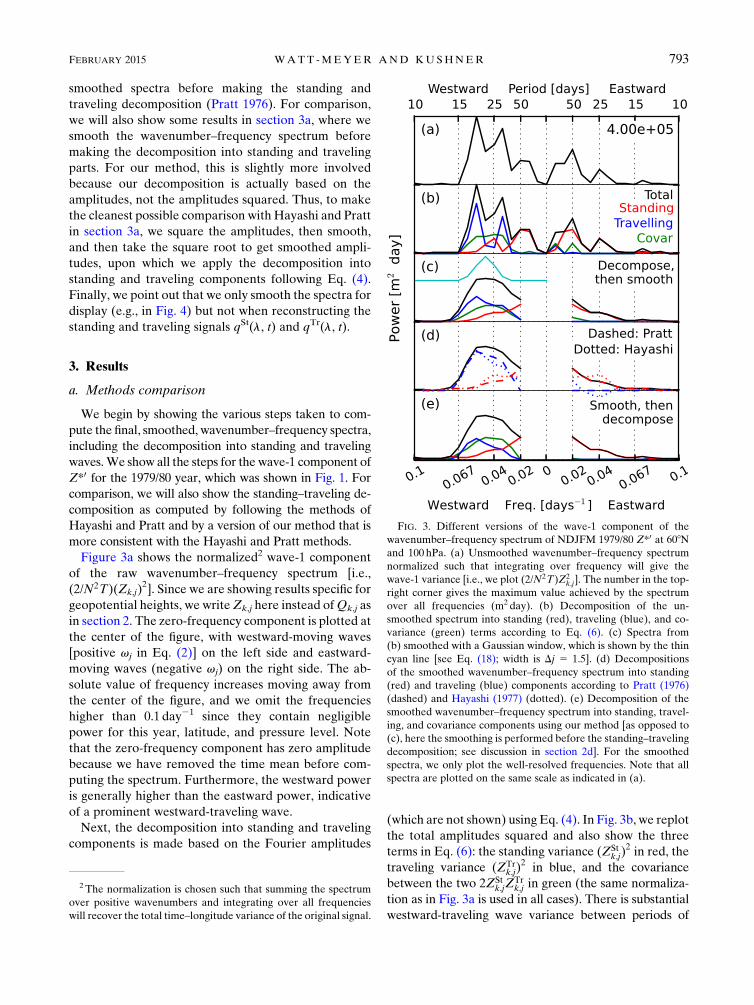
Figure 3a shows the normalized2 wave-1 component
of the raw wavenumber–frequency spectrum [i.e.,
(2/N2T)(Zk,j)2]. Since we are showing results specific for
geopotential heights, we writeZk,j here instead ofQk,j as
in section 2. The zero-frequency component is plotted at
the center of the figure, with westward-moving waves
[positive vj in Eq. (2)] on the left side and eastward-
moving waves (negative vj) on the right side. The ab-
solute value of frequency increases moving away from
the center of the figure, and we omit the frequencies
higher than 0.1 day21 since they contain negligible
power for this year, latitude, and pressure level. Note
that the zero-frequency component has zero amplitude
because we have removed the time mean before com-
puting the spectrum. Furthermore, the westward power
is generally higher than the eastward power, indicative
of a prominent westward-traveling wave.
Next, the decomposition into standing and traveling
components is made based on the Fourier amplitudes
(which are not shown) using Eq. (4). In Fig. 3b, we replot
the total amplitudes squared and also show the three
terms in Eq. (6): the standing variance (ZStk,j)
2 in red, the
traveling variance (ZTrk,j)
2 in blue, and the covariance
between the two 2ZStk,jZ
Trk,j in green (the same normaliza-
tion as in Fig. 3a is used in all cases). There is substantial
westward-traveling wave variance between periods of
FIG. 3. Different versions of the wave-1 component of the
wavenumber–frequency spectrum of NDJFM 1979/80 Z*0 at 608Nand 100 hPa. (a) Unsmoothed wavenumber–frequency spectrum
normalized such that integrating over frequency will give the
wave-1 variance [i.e., we plot (2/N2T)Z2k,j]. The number in the top-
right corner gives the maximum value achieved by the spectrum
over all frequencies (m2 day). (b) Decomposition of the un-
smoothed spectrum into standing (red), traveling (blue), and co-
variance (green) terms according to Eq. (6). (c) Spectra from
(b) smoothed with a Gaussian window, which is shown by the thin
cyan line [see Eq. (18); width is Dj 5 1.5]. (d) Decompositions
of the smoothed wavenumber–frequency spectrum into standing
(red) and traveling (blue) components according to Pratt (1976)
(dashed) and Hayashi (1977) (dotted). (e) Decomposition of the
smoothed wavenumber–frequency spectrum into standing, travel-
ing, and covariance components using our method [as opposed to
(c), here the smoothing is performed before the standing–traveling
decomposition; see discussion in section 2d]. For the smoothed
spectra, we only plot the well-resolved frequencies. Note that all
spectra are plotted on the same scale as indicated in (a).
2 The normalization is chosen such that summing the spectrum
over positive wavenumbers and integrating over all frequencies
will recover the total time–longitude variance of the original signal.
FEBRUARY 2015 WATT -MEYER AND KUSHNER 793
15–30 days, while standing waves dominate at the lowest
frequencies. We also have the expected properties that
ZStk,j 5ZSt
k,2j and that eitherZTrk,j 5 0 orZTr
k,2j 5 0. Next, we
smooth each of the terms individually, as discussed in
section 2d. The smoothed spectra, as well as theGaussian
window used to do the smoothing, are plotted in Fig. 3c.
We also compare with the methods described by von
Storch and Zwiers (1999), which are based on those in
Pratt (1976) and Hayashi (1977). However, as noted in
section 2c, the Pratt method described in von Storch and
Zwiers (1999) is actually a conflation of the true Pratt
and Hayashi methods. For the remainder of the paper,
when we discuss the ‘‘Pratt’’ method, we refer to the
method attributed to Pratt that is described in section
11.5.7 of von Storch and Zwiers (1999).
In Fig. 3d, the decompositions described by Pratt and
Hayashi are shown. The variance is exclusively decom-
posed into standing and traveling portions, without any
covariance. Furthermore, note that these authors sug-
gest computing a smoothed wavenumber–frequency
spectrum before making the decomposition into stand-
ing and traveling components. This is what has been
done in Fig. 3d, and so for comparison, in Fig. 3e we
show the results for our decomposition based on the
presmoothed total spectrum (see discussion in section
2d). Our method gives identical results for the standing
wave power as the Pratt method when consistent
smoothing is done, and the Hayashi standing wave power
is generally similar. However, both Pratt and Hayashi
attribute the remaining variance exclusively to the trav-
eling wave, whereas we assign it to both the traveling
wave and the covariance between the standing and trav-
eling waves. This leads to a major reduction in the vari-
ance attributed exclusively to the traveling wave in our
method. Also, note that Hayashi’s method gives a nega-
tive traveling wave power at some frequencies—a clearly
nonphysical result.
b. Reconstruction of standing and traveling wavefields
Using Eqs. (2) and (3) with the decomposed ampli-
tudes QStk,j and QTr
k,j replacing the total amplitudes Qk,j,
one can reconstruct the standing and traveling parts of
the signal q(l, t). To accurately reconstruct the original
signal, it is necessary to use the unsmoothed amplitudes.
In the two right columns of Fig. 1, the wave-1 portions of
the standing and traveling signals are plotted for 608Nand 100 hPa for the 1979/80 and 1990/91 winters. As we
had expected from viewing the total wave-1 anomaly, the
1979/80 year contains a consistent westward-propagating
wave. However, the quantitative decomposition that we
make allows us to also recognize the significant contri-
bution of standing waves to the variability this year. For
the 1990/91 year, we see the expected result: the stand-
ing wave field looks very similar to the total field, while
the traveling wave field generally has small amplitudes.
Note that the standing and travelingwave reconstructions
are not ‘‘pure’’ standing or traveling waves because they
are the combination of a range of frequencies. As well,
since the method naturally focuses on explaining the
largest-variance features, in some cases it is possible for
the technique to generate somewhat spurious results in
the low-amplitude part of the signal. For example, in
Fig. 1, the standing part of the signal for mid-November–
December 1990 contains an eastward-propagating fea-
ture. Nevertheless, it is of much smaller amplitude than
the standing wave feature later in the season, which is
accurately captured.
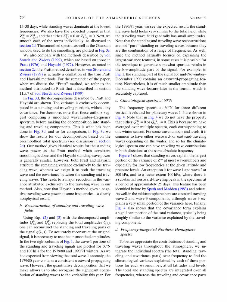
c. Climatological spectra at 608N
The frequency spectra at 608N for three different
vertical levels and for planetary waves 1–3 are shown in
Fig. 4. Note that in Fig. 4 we do not have the property
that eitherQTrk,j 5 0 orQTr
k,2j 5 0. This is because we have
averaged over multiple spectra, each corresponding to
one winter season. For somewavenumbers and levels, it is
common to have either westward- or eastward-traveling
waves depending on the winter, and so for the climato-
logical spectra one can have traveling wave contributions
in both directions at the same absolute frequency.
Figure 4 shows that standing waves explain the largest
portion of the variance of Z*0 at most wavenumbers and
especially for low frequencies at the given latitude and
pressure levels. An exception is for wave 1 and wave 2 at
500 hPa, and to a lesser extent 100 hPa, where there is
a substantial westward-traveling peak in the spectrum at
a period of approximately 25 days. This feature has been
identified before by Speth and Madden (1983) and others.
Aswell, in themidstratosphere there are eastward-traveling
wave-2 and wave-3 components, although wave 3 ex-
plains a very small portion of the variance here. Finally,
Fig. 4 also shows that the covariance term explains
a significant portion of the total variance, typically being
roughly similar to the variance explained by the travel-
ing component.
d. Frequency-integrated Northern Hemispherespectra
To better appreciate the contributions of standing and
traveling waves throughout the atmosphere, we in-
tegrate the individual spectra (the total, standing, trav-
eling, and covariance parts) over frequency to find the
climatological variance explained by each of these por-
tions for each wavenumber, at all latitudes and levels.
The total and standing spectra are integrated over all
frequencies, whereas the traveling and covariance parts
794 JOURNAL OF THE ATMOSPHER IC SC IENCES VOLUME 72

are integrated separately over negative and positive
frequencies to isolate the eastward and westward com-
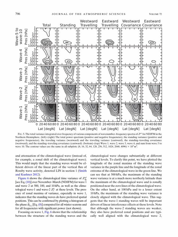
ponents. These quantities are shown for the Northern
Hemisphere in Fig. 5. We separately show the contri-
butions bywaves 1–4 and sum together the contributions
from waves 5–10. Note the logarithmic scale for the
contours: each contour represents a doubling of vari-
ance. Furthermore, in each row, the five right panels
summed together give the leftmost panel.
The most important points to take from Fig. 5 are the
following. As expected by the Charney–Drazin criteria,
the stratospheric anomalies are dominated by wave 1 and
wave 2 and, to a lesser extent, wave 3. In the stratosphere,
the standing waves typically explain about half the total
variance and the remaining variance is distributed
roughly equally between the four remaining categories
for wave 1, while for waves 2 and 3 there is more power in
the eastward-traveling and covariance parts than in the
westward parts. In the troposphere there is a largely dif-
ferent distribution of variance. In terms of wavenumber,
the maximum contribution depends on the latitude: at
very high latitudes (north of 758) wave 1makes the largest
contribution, while moving to lower latitudes, larger
wavenumbers tend to make relatively larger contribu-
tions. Furthermore, at very high latitudes standing waves
explain amajority of the variance ofwave 1, while between
608 and 808N there is a substantial westward-traveling
and covariance contribution. This was noted previously
in Fig. 4. Moving to higher wavenumbers, there is
generally a diminishing contribution from standing
waves and an increase in the variance explained by
eastward-propagating waves instead of westward-
propagating waves, as we expect from the simple b-plane
Rossby wave dispersion relation. For synoptic-scale dis-
turbances (waves 5–10), the majority of the variance is
explained by eastward-traveling waves in the midlatitudes,
as expected.
The westward and eastward covariance portions, in
the two right columns of Fig. 5, are generally similar in
structure and amplitude to the respective westward- and
eastward-traveling variances. We do not necessarily ex-
pect to find any independent information in the covari-
ance plot: by the construction of the standing–traveling
decomposition, the covariance between the two wave
structures at some wavenumber and frequency is entirely
determined by the amplitudes (or variances) of the in-
dividual standing and traveling parts [see Eq. (6)].
e. Relative structure of standing and climatologicalwave
Having established the importance of standing waves
throughout the extratropical atmosphere, we now seek
to understand their zonal structure. In particular, we
wish to know whether the nodes and antinodes of these
standing waves have preferred longitudinal positions. If
so, and if the antinodes are in alignment with the max-
imum andminimum of the climatological wave, then the
standing waves will primarily be driving amplification
FIG. 4. The climatological wavenumber–frequency spectrum ofZ*0 for NDJFM at 608N and (left) 500, (middle) 100, and (right) 10 hPa.
Black is (Zk,j)2, red is (ZSt
k,j)2, blue is (ZTr
k,j)2, and green is 2ZSt
k,jZTrk,j. Only the first three wavenumbers and periods to 6 days are shown.
Smoothing is as in Fig. 3c. All wavenumbers and levels are plotted using different scales, which are shown in the top-right corner of each
plot, indicating the maximum value (m2 day) reached by the total spectrum for that wavenumber and level. The spectra are normalized by
2/N2T so that integrating over frequency and summing over wavenumber will recover the total variance of the original signal.
FEBRUARY 2015 WATT -MEYER AND KUSHNER 795
and attenuation of the climatological wave (instead of,
for example, a zonal shift of the climatological wave).
This would imply that the standing waves would be ef-
ficient drivers of the linear part of the vertical flux of
Rossby wave activity, denoted LIN in section 1 (Smith
and Kushner 2012).
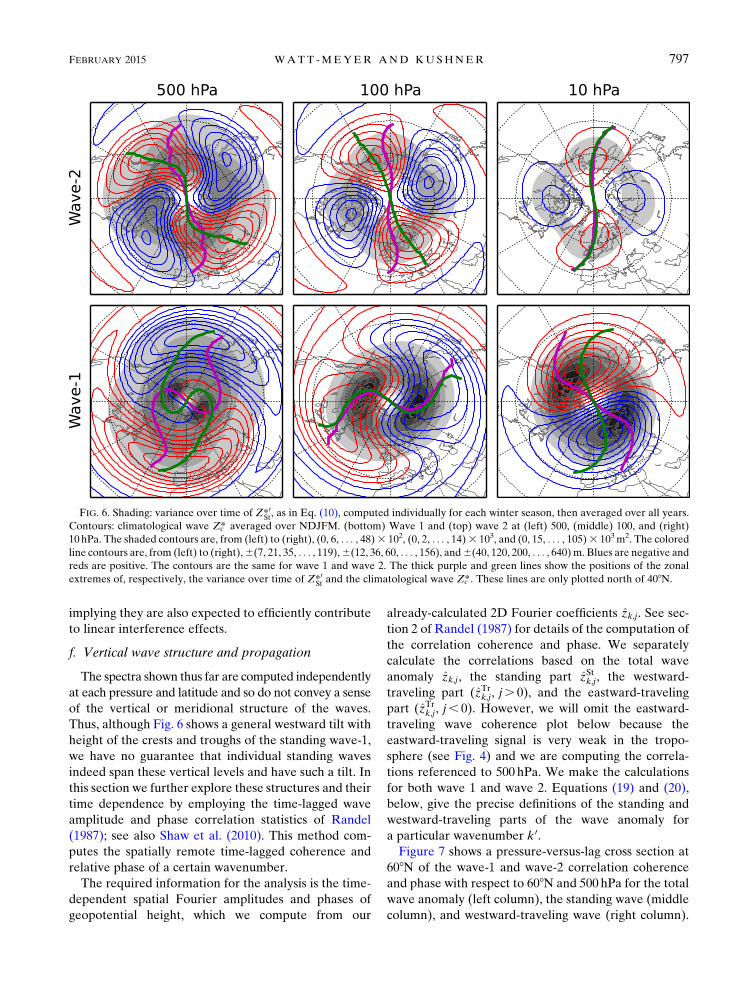
Figure 6 shows the climatological time variance of Z*0St
[seeEq. (10)] overNovember–March (NDJFM) forwave 1
and wave 2 at 500, 100, and 10hPa, as well as the clima-
tological wave-1 and wave-2 Zc* at these levels. The pres-
ence of zonal maxima of variance, especially in wave 1,
indicates that the standing waves do have preferred spatial
positions. This can be confirmed by plotting a histogram of
the phasefk,j [Eq. (8)] computed for all winter seasons and
for all frequencies with significant power (not shown).
Focusing on wave 1, Fig. 6 shows that the relationship
between the structure of the standing waves and the
climatological wave changes substantially at different
vertical levels. To clarify this point, we have plotted the
longitude of the zonal maxima of the standing wave
variance in the purple line and the longitude of the zonal
extrema of the climatological wave in the green line. We
can see that at 500 hPa, the maximum of the standing
wave variance is at a much more northerly latitude than
the maximum of the climatological wave and is zonally
positioned near the zero lines of the climatological wave.
On the other hand, at 100 hPa and to a lesser extent
10 hPa, the maximum of the standing wave variance is
closely aligned with the climatological wave. This sug-
gests that the wave-1 standing waves will be important
drivers of linear interference effects at these levels. Note
that although the wave-2 standing waves are weaker,
they also have preferred zonal positions and are typi-
cally well aligned with the climatological wave 2,
FIG. 5. The total variance integrated over frequency of various components of wavenumber–frequency spectra ofZ*0 for NDJFM in the
Northern Hemisphere. (left)–(right) The total power spectrum (positive and negative frequencies), the standing variance (positive and
negative frequencies), the traveling variance (westward) and the traveling variance (eastward), the standing–traveling covariance
(westward), and the standing–traveling covariance (eastward). (bottom)–(top) Wave 1, wave 2, wave 3, wave 4, and sum from wave 5 to
wave 10. The contour values are the same in all subplots: (8, 16, 32, 64, 128, 256, 512, 1024, 2048, 4096) 3 102m2.
796 JOURNAL OF THE ATMOSPHER IC SC IENCES VOLUME 72
implying they are also expected to efficiently contribute
to linear interference effects.
f. Vertical wave structure and propagation
The spectra shown thus far are computed independently
at each pressure and latitude and so do not convey a sense
of the vertical or meridional structure of the waves.
Thus, although Fig. 6 shows a general westward tilt with
height of the crests and troughs of the standing wave-1,
we have no guarantee that individual standing waves
indeed span these vertical levels and have such a tilt. In
this section we further explore these structures and their
time dependence by employing the time-lagged wave
amplitude and phase correlation statistics of Randel
(1987); see also Shaw et al. (2010). This method com-
putes the spatially remote time-lagged coherence and
relative phase of a certain wavenumber.
The required information for the analysis is the time-
dependent spatial Fourier amplitudes and phases of
geopotential height, which we compute from our
already-calculated 2D Fourier coefficients zk,j. See sec-
tion 2 of Randel (1987) for details of the computation of
the correlation coherence and phase. We separately
calculate the correlations based on the total wave
anomaly zk,j, the standing part zStk,j, the westward-
traveling part (zTrk,j, j. 0), and the eastward-traveling
part (zTrk,j, j, 0). However, we will omit the eastward-
traveling wave coherence plot below because the
eastward-traveling signal is very weak in the tropo-
sphere (see Fig. 4) and we are computing the correla-
tions referenced to 500 hPa. We make the calculations
for both wave 1 and wave 2. Equations (19) and (20),
below, give the precise definitions of the standing and
westward-traveling parts of the wave anomaly for
a particular wavenumber k0.Figure 7 shows a pressure-versus-lag cross section at
608N of the wave-1 and wave-2 correlation coherence
and phase with respect to 608N and 500 hPa for the total
wave anomaly (left column), the standing wave (middle
column), and westward-traveling wave (right column).
FIG. 6. Shading: variance over time of Z*0St, as in Eq. (10), computed individually for each winter season, then averaged over all years.
Contours: climatological wave Zc* averaged over NDJFM. (bottom) Wave 1 and (top) wave 2 at (left) 500, (middle) 100, and (right)
10 hPa. The shaded contours are, from (left) to (right), (0, 6, . . . , 48)3 102, (0, 2, . . . , 14)3 103, and (0, 15, . . . , 105)3 103m2. The colored
line contours are, from (left) to (right),6(7, 21, 35, . . . , 119),6(12, 36, 60, . . . , 156), and6(40, 120, 200, . . . , 640)m. Blues are negative and
reds are positive. The contours are the same for wave 1 and wave 2. The thick purple and green lines show the positions of the zonal
extremes of, respectively, the variance over time of Z*0Stand the climatological wave Zc*. These lines are only plotted north of 408N.
FEBRUARY 2015 WATT -MEYER AND KUSHNER 797

Shaw et al. (2010), using a shorter dataset and hence
fewer degrees of freedom, estimate that coherences
above 0.18 are statistically significant at the 99% level.
We only plot coherences of 0.2 or above and are thus
assured that the coherences shown are all significant at
least at the 99% level. Focusing first on the total wave-1
anomalies (Fig. 7d), we see evidence for the well-known
upward propagation of wave 1: for positive 3–6-day lags,
there is a strong (.0.3) coherence between wave am-
plitudes at 10 hPa and the reference point at 500 hPa.
Furthermore, at 0-day and positive lags, the wave 1 has
a westward tilt with height throughout the upper tro-
posphere and stratosphere—further evidence for the
upward propagation of the wave. There is a suggestion
of downward propagation for negative lags in the phase
diagram (eastward phase tilt with height) but no such
indication in the coherence diagram. This is partially due
to using the entire NDJFM period to compute the cor-
relations: as shown in Shaw et al. (2010), wave reflection
has a strong seasonal cycle and peaks in strength in
January–March (JFM). Furthermore, stronger cou-
plings to the stratosphere, both upward and downward,
are seen if ameridional average [e.g., from 458 to 808Nas
in Shaw et al. (2010)] is performed before computing the
correlations. We choose to perform the correlations
based on 608N for easy comparison with results we have
already shown based solely on this latitude (e.g., in
Figs. 1 and 4). Last, we note the clear tendency of
westward propagation of wave 1 throughout the tropo-
sphere, as seen in the steadily decreasing phase with lag
in Fig. 7d. Generally, the same conclusions can be
reached for the total wave-2 signal (Fig. 7a) except that
the time scale for upward propagation is faster (2–3
days) and there is no eastward phase tilt with height at
negative lags.
Now we examine the correlations separately for the
standing and westward-traveling parts of the wave-1 and
wave-2 geopotential height anomalies, which are spe-
cifically given by (for some wavenumber k0)
zStk0 (l, t)52
NT�T2
j52T2
ZStk0 , j cos(k
0l1vjt1fk0, j) and
(19)
zTrWk0 (l, t)52
NT�j51
T2
ZTrk0, j cos(k
0l1vjt1fk0, j) . (20)
Here,ZStk0,j andZ
Trk0 ,j are respectively the wave-k
0 standingand traveling amplitudes of the geopotential height
FIG. 7. Correlation coherence (contours) and phase (shading) of (a)–(c) wave-2 and (d)–(f) wave-1 geopotential height anomalies
during NDJFMat 608N as a function of pressure and lag with respect to 608N and 500hPa. Correlations are computed using (left) the total
wave anomaly, (middle) only the standing part, and (right) only the westward-traveling part [see Eqs. (19) and (20)]. The coherence is
plotted at intervals of 0.1, starting from 0.2. The phase (8) denotes the longitudinal separation of the two wave crests: positive phasemeans
the distant (away from 0-day lag and 500hPa) wave is eastward of the reference wave.
798 JOURNAL OF THE ATMOSPHER IC SC IENCES VOLUME 72

anomaly at frequencyvj and fk0,j is the wave-k0 phase at
frequency vj. Note that in Eq. (20) we sum over only
positive j in order to isolate the westward-traveling
waves.
Examining Fig. 7e, we see that for wave 1 the standing
wave coherence is similar to the total wave coherence,
but with generally smaller coherences throughout. The
correlation phase for the standing wave is analogous to
that for the total wave, but without the westward propa-
gation in the troposphere. In addition, the westward and
eastward phase tilts with height for positive and negative
lags tend to be more extreme for the standing wave as
compared to the total wave. As expected from the defi-
nition of the standing wave, at 500hPa we see essentially
no change in the phase of the wave with time for the lags
shown, although at approximately614 days (not shown)
there is a sharp 1808 jump in phase, which would be in
accordance with a standing wave with a 28-day period.
For wave 2 (Fig. 7b), there is a very close correspondence
between the coherence plots of the standing and wave
and the total wave, and there is no change in phase until
lags of 610 days.
The westward-propagating wave-1 and wave-2
anomalies (Figs. 7c and 7f) are vertically deep signals,
spanning the troposphere and up to the midstrato-
sphere at 0-day lag, with an equivalent barotropic
structure in the troposphere and weak westward phase
tilts with height in the stratosphere. Furthermore, they
have amuch longer coherence time scale (0.2 coherence
up to 613 days at 500 hPa for wave 1) compared to the
total wave in both in the troposphere and in the
stratosphere. The correlation phases show the expected
consistent phase propagation, with a 3608 revolution at
500 hPa beingmade in about 28 days for wave 1, roughly
in accordance with the westward-traveling wave-1
spectral peak seen in the left panel of Fig. 4. These re-
sults agree with the vertical structure of Northern
Hemisphere high-latitude westward-propagating wave-1
features identified by previous authors—for example,
Fig. 11 of Branstator (1987) or Fig. 7 of Madden and
Speth (1989). The eastward-traveling signals (not
shown) are strongly trapped in the troposphere and the
progression of phase is not as consistent as for the
westward-traveling wave.
Note that largely the same conclusions can be reached
by picking a reference point in the stratosphere—for
example, at 608N and 10 hPa (not shown). The standing
wave amplitudes here are preceded by anomalies in the
troposphere about 3–6 days before for wave 1 (less for
wave 2), and the westward-propagating waves fill the
depth of the stratosphere and troposphere with a baro-
tropic structure in the troposphere and a slight westward
tilt with height in the stratosphere. The eastward waves
referenced to the stratosphere do not penetrate into the
troposphere.
4. Summary and discussion
In this studywehave introduced a novel decomposition
of longitude- and time-dependent signals into standing
and traveling components. Unlike previous techniques,
ourmethod explicitly provides the covariance between the
standing and traveling waves and permits reconstruction
of the standing and traveling signals. We apply the de-
composition to geopotential height anomalies in the
Northern Hemisphere winter. Focusing on planetary
waves 1–3, we find that at 608N the standing wave explains
the largest portion of the variance in wave anomalies, es-
pecially at low frequencies. There are exceptions for wave
1 and to a lesser extent wave 2, which have substantial
westward-traveling anomalies in the troposphere with
periods around 25 days. In the stratosphere standingwaves
generally dominate, except for a small peak in the
eastward-traveling wave 2 with a period of about 16 days.
We have also shown that planetary wave-1 and wave-2
standing wave anomalies have preferred longitudinal posi-
tions and that their antinodes generally align with the max-
imumandminimumof the climatologicalwave, especially in
the lower and midstratosphere. This implies that the stand-
ing waves should be an efficient driver of LIN (Smith and
Kushner 2012), which is the vertical flux of Rossby wave
activity that is linearly dependent on the climatological wave
pattern. This point will be examined in more detail in
a subsequent paper. Last, we examined the vertical and
time-lagged structure of the standing and traveling wave-1
and wave-2 signals with respect to 608N and 500hPa. We
found that the standing waves have a similar structure to the
total wavewith a tendency for upward propagation from the
troposphere to the stratospherewith a time scaleof 3–6 (2–3)
days for wave 1 (wave 2). On the other hand, the westward-
traveling wave 1 and wave 2 are deep signals spanning the
troposphere and stratosphere with relatively little phase tilt.
The separation of wave anomalies into standing and
traveling parts is helpful for distinguishing the wave
events that originate in the troposphere and drive
stratospheric variability. Although, as we have shown,
the westward-propagating wave 1 is a strong feature in
the high-latitude troposphere and lower stratosphere;
because of its lack of phase tilt, we do not expect it to
strongly contribute to the vertical flux of wave activity.
On the other hand, we have isolated standing waves and
shown that they have a tendency to strengthen and
weaken the climatological wave. In addition, the phase
tilts and time-lagged coherences of the standing wave
contributions are suggestive of upward propagation, and
one would expect them to be responsible for the upward
FEBRUARY 2015 WATT -MEYER AND KUSHNER 799
communication of wave activity anomalies from the tro-
posphere to stratosphere. Future work will quantify the
contributions of the standing and traveling waves to wave
activity flux variability over a range of time scales.
Acknowledgments. The authors thank Dr. Karen
L. Smith for discussions during O.W.’s visit to the Lamont–
Doherty Earth Observatory in 2013. We are also grateful
for helpful comments from three anonymous reviewers. The
authors acknowledge funding from the Natural Sciences
and Engineering Research Council of Canada, the Ontario
Graduate Scholarship program, and the Centre for Global
Change Science at theUniversity of Toronto. P. J. K. wishes
to acknowledge helpful feedback received during the Kavli
Institute for Theoretical Physics ‘‘Wave-Flow Interaction’’
program in 2014. This research was supported in part by the
National Science Foundation under Grant PHY11-25915.
APPENDIX
Spectral Identities and Derivations
a. Inverse Fourier transform of real signal
The inverse 2D discrete Fourier transform is con-
ventionally written as
q(l, t)51
NT�N21
k51�T21
j50
eikl1ivjtqk, j . (A1)
Noting that qk,j 5 qN1k,T1j and assuming for conve-
nience that N and T are odd (which is not strictly nec-
essary), one can rewrite Eq. (A1) as
q(l, t)51
NT�N
2
k52N2
�T
2
j52T2
eikl1ivjt qk, j , (A2)
whereN25 (N2 1)/2 and T25 (T2 1)/2. Furthermore,
given that q(l, t) is a real-valued function, we have
q2k,2j 5 (qk,j)y, where the dagger represents the com-
plex conjugate. Thus, we can keep only half the Fourier
coefficients. Recalling that q(l, t) has zero zonal mean,
we can rewrite Eq. (A2) as
q(l, t)51
NT�N
2
k51�T2
j52T2
eikl1ivjtqk, j
11
NT�21
k52N2
�T2
j52T2
eikl1ivjtqk, j . (A3)
Then, using that
�21
k52N2
�T
2
j52T2
eikl1ivjt qk,j 5 �
N2
k51�T2
j52T2
e2ikl1ivjt q2k,j
5 �N
2
k51�T2
j52T2
e2ikl2ivjt q2k,2j
5
�N
2
k51�T
2
j52T2
eikl1ivjt qk,j
!y,
(A4)
where the second equality holds because we are sum-
ming over a symmetric (about zero) range of integers j,
we see
q(l, t)52
NT�N
2
k51�T2
j52T2
Re(eikl1ivjtqk,j) . (A5)
Rewriting the Fourier coefficients in terms of their am-
plitudes and complex phases, qk,j 5Qk,jeifk,j , we have
our reformulated inverse 2D discrete Fourier transform:
q(l, t)52
NT�N
2
k51�T2
j52T2
Qk,j cos(kl1vjt1fk,j) . (A6)
It is trivial to rewrite this in the form of Eq. (2) given that
q(l, t) as zero time mean.
b. Longitude of standing wave antinodes
Hayashi (1973, 1977) and Pratt (1976) provide a for-
mula for computing the longitudes of the antinodes of the
standing part of a signal in terms of the power spectra and
cross-spectra of ck(t) and sk(t) (note, in this section, that
we follow the notation of Hayashi and Pratt, as outlined
in section 2c). In particular, Hayashi (1973) defines3
a5 tan21
"2Kv(ck, sk)
Pv(ck)2Pv(sk)
#(A7)
and shows that the longitudes of the maximum time
variance of the signal are given by
l5mp1a/2
k, (A8)
where m is an integer. We showed in section 2a that
the longitudes of the antinodes of the standing wave
at wavenumber k and frequency vj are given by
3Note Eq. (3.3) in Hayashi (1973) is erroneously missing the
tan21. See, for example, Eq. (13) of Pratt (1976) or Eq. (4.3) of
Hayashi (1977).
800 JOURNAL OF THE ATMOSPHER IC SC IENCES VOLUME 72

l5 (1/k)(mp2fk,j) with fk,j defined in Eq. (8). Thus, to
demonstrate the equivalence between our formula and
Hayashi’s, we must show that a522fk,j.
We begin by rewriting Eq. (7) in the form of Eq. (13).
Note for simplicity we take QStk,j 5 1, although the deri-
vation holds generally. Straightforward algebraic ma-
nipulations can be used to show that
qStk,6j(l, t)5 ck(t) coskl1 sk(t) sinkl , (A9)
where
ck(t)5 (cosfk,j 1 cosfk,2j) cosvjt
1 (2sinfk,j 1 sinfk,2j) sinvjt (A10)
and
sk(t)5 (2sinfk, j2 sinfk,2j) cosvjt
1 (2cosfk, j 1 cosfk,2j) sinvjt . (A11)
We now compute the Fourier transforms of ck(t) and
sk(t) in order to be able to compute their power
spectra and cross-spectra. That is, we decompose ck(t)
and sk(t) as
ck(t)5 ck,jeiv
jt 1 ck,2je
2ivjt and (A12)
sk(t)5 sk,jeiv
jt 1 sk,2je
2ivjt , (A13)
where
ck,j51
2(cosfk,j1 cosfk,2j 1 i sinfk,j 2 i sinfk,2j) ,
(A14)
sk,j 51
2(2sinfk,j 2 sinfk,2j 1 i cosfk,j 2 i cosfk,2j) ,
(A15)
and ck,2j 5 (ck,j)y and sk,2j 5 (sk,j)
y. Using these formu-
las, one can show that
Pv(ck)5 jck,jj25 cos2�fk,j 1fk,2j
2
�, (A16)
Pv(sk)5 jsk,jj25 sin2�fk,j1fk,2j
2
�, and (A17)
Kv(ck, sk)5Re(ck,jsk,j)521
2sin(fk,j 1fk,2j) . (A18)
Thus, substituting the above into Eq. (A7) we have that
a5 tan21
8<:
2sin(fk,j1fk,2j)
cos2[(fk,j1fk,2j)/2]2 sin2[(fk,j1fk,2j)/2]
9=;
52tan21
24 sin(fk,j1fk,2j)
cos(fk,j1fk,2j)
35
52(fk,j1f2k,j)522fk, j
(A19)
as required.
c. Variance over time
Here, we show how the variance over time of a single-
wavenumber signal can be rewritten as a sum over the
Fourier coefficients. We consider
qk(l, t)52
NT�T
2
j52T2
Qk,j cos(kl1vjt1fk,j) . (A20)
We compute the variance over time of the single-
wavenumber signal (assuming the time mean is zero)—
a quantity that depends on longitude:
var(qk)(l)51
T�T21
t50
[qk(l, t)]2
54
N2T3 �T
2
j52T2
�T2
j052T2
Qk,jQk,j0
3 �T21
t50
cos(kl1vjt1fk,j)cos(kl1vj0 t1fk,j0),
(A21)
where we have substituted in Eq. (A20) and then
changed the order of summation. Using the orthogo-
nality of the cosine basis functions, one can show
�T21
t50
cos(kl1vjt1fk,j) cos(kl1vj0 t1fk,j0)
5T
2dj,j0 1
T
2cos(2kl1 2fk,j)dj,2j0
5T
2dj,j0 1
T
2[2 cos2(kl1fk,j)2 1]dj,2j0 . (A22)
Substituting Eq. (A22) into Eq. (A21) we have our final
result for the variance over time of our signal repre-
sented as a sum over the Fourier coefficients:
FEBRUARY 2015 WATT -MEYER AND KUSHNER 801

var(qk)(l)52
N2T2 �T2
j52T2
[Q2k,j1 2Qk,jQk,2j cos
2(kl1fk,j)2Qk,jQk,2j] . (A23)
REFERENCES
Baldwin, M. P., and T. J. Dunkerton, 2001: Stratospheric harbin-
gers of anomalous weather regimes. Science, 294, 581–584,
doi:10.1126/science.1063315.
Branstator, G., 1987:A striking example of the atmosphere’s leading
traveling pattern. J. Atmos. Sci., 44, 2310–2323, doi:10.1175/
1520-0469(1987)044,2310:ASEOTA.2.0.CO;2.
Dee, D. P., and Coauthors, 2011: The ERA-Interim reanalysis:
Configuration and performance of the data assimilation
system.Quart. J. Roy. Meteor. Soc., 137, 553–597, doi:10.1002/
qj.828.
Di Biagio, V., S. Calmanti, A. Dell’Aquila, and P. M. Ruti, 2014:
Northern Hemisphere winter midlatitude atmospheric vari-
ability in CMIP5 models. Geophys. Res. Lett., 41, 1277–1282,
doi:10.1002/2013GL058928.
Fraedrich, K., andH.Böttger, 1978:Awavenumber-frequency analysis
of the 500mb geopotential at 508N. J. Atmos. Sci., 35, 745–750,
doi:10.1175/1520-0469(1978)035,0745:AWFAOT.2.0.CO;2.
Garfinkel, C., D. Hartmann, and F. Sassi, 2010: Tropospheric
precursors of anomalous Northern Hemisphere stratospheric
polar vortices. J. Climate, 23, 3282–3299, doi:10.1175/
2010JCLI3010.1.
Haurwitz, B., 1940: The motion of atmospheric disturbances on
a spherical earth. J. Mar. Res., 3, 254–267.
Hayashi, Y., 1971: A generalized method of resolving disturbances
into progressive and retrogressive waves by space Fourier and
time cross-spectral analyses. J. Meteor. Soc. Japan, 49, 125–128.
——, 1973: A method of analyzing transient waves by space-time
cross spectra. J. Appl. Meteor., 12, 404–408, doi:10.1175/
1520-0450(1973)012,0404:AMOATW.2.0.CO;2.
——, 1977: On the coherence between progressive and retrogres-
sive waves and a partition of space-time power spectra into
standing and traveling parts. J. Appl. Meteor., 16, 368–373,
doi:10.1175/1520-0450(1977)016,0368:OTCBPA.2.0.CO;2.
——, 1979: A generalized method of resolving transient distur-
bances into standing and traveling waves by space-time spec-
tral analysis. J. Atmos. Sci., 36, 1017–1029.
Lucarini, V., S. Calmanti, A. Dell’Aquila, P. M. Ruti, and
A. Speranza, 2007: Intercomparison of the northern hemisphere
winter midlatitude atmospheric variability of the IPCC models.
Climate Dyn., 28, 829–848, doi:10.1007/s00382-006-0213-x.Madden, R. A., 1979: Observations of large-scale traveling Rossby
waves.Rev. Geophys. Space Phys., 17, 1935–1949, doi:10.1029/
RG017i008p01935.
——, and P. Speth, 1989: The average behavior of large-scale
westward traveling disturbances evident in the Northern
Hemisphere geopotential heights. J. Atmos. Sci., 46, 3225–3239,
doi:10.1175/1520-0469(1989)046,3225:TABOLS.2.0.CO;2.
May, W., 1999: Space-time spectra of the atmospheric intra-
seasonal variability in the extratropics and their dependency
on the El Niño/Southern Oscillation phenomenon: Modelversus observation. Climate Dyn., 15, 369–387, doi:10.1007/
s003820050288.
Nishii, K., H. Nakamura, and T. Miyasaka, 2009: Modulations in
the planetary wave field induced by upward-propagating
Rossby wave packets prior to stratospheric sudden warming
events: A case study. Quart. J. Roy. Meteor. Soc., 135, 39–52,
doi:10.1002/qj.359.
Pratt, R. W., 1976: The interpretation of space-time spectral
quantities. J. Atmos. Sci., 33, 1060–1066, doi:10.1175/
1520-0469(1976)033,1060:TIOSTS.2.0.CO;2.
Randel, W. J., 1987: A study of planetary waves in the southern
winter troposphere and stratosphere. Part I: Wave structure and
vertical propagation. J. Atmos. Sci., 44, 917–935, doi:10.1175/
1520-0469(1987)044,0917:ASOPWI.2.0.CO;2.
——, and I. M. Held, 1991: Phase speed spectra of transient eddy
fluxes and critical layer absorption. J. Atmos. Sci., 48, 688–697,
doi:10.1175/1520-0469(1991)048,0688:PSSOTE.2.0.CO;2.
Shaw, T. A., J. Perlwitz, and N. Harnik, 2010: Downward wave
coupling between the stratosphere and troposphere: The im-
portance of meridional wave guiding and comparison with
zonal-mean coupling. J. Climate, 23, 6365–6381, doi:10.1175/
2010JCLI3804.1.
Smith, K. L., and P. J. Kushner, 2012: Linear interference and
the initiation of extratropical stratosphere-troposphere in-
teractions. J. Geophys. Res., 117, D13107, doi:10.1029/
2012JD017587.
Speth, P., and R. A. Madden, 1983: Space-time spectral anal-
yses of Northern Hemisphere geopotential heights. J. Atmos.
Sci., 40, 1086–1100, doi:10.1175/1520-0469(1983)040,1086:
STSAON.2.0.CO;2.
Tsay, C.-Y., 1974:A note on themethods of analyzing travelingwaves.
Tellus, 26, 412–415, doi:10.1111/j.2153-3490.1974.tb01619.x.
von Storch, H., and F. W. Zwiers, 1999: Statistical Analysis in Cli-
mate Research. Cambridge University Press, 494 pp.
Wheeler, M., and G. N. Kiladis, 1999: Convectively coupled
equatorial waves: Analysis of clouds and temperatures in the
wavenumber–frequency domain. J. Atmos. Sci., 56, 374–399,
doi:10.1175/1520-0469(1999)056,0374:CCEWAO.2.0.CO;2.
Zhang, C., and H. H. Hendon, 1997: Propagating and standing com-
ponents of the intraseasonal oscillation in tropical convection.
J.Atmos. Sci., 54, 741–752, doi:10.1175/1520-0469(1997)054,0741:
PASCOT.2.0.CO;2.
802 JOURNAL OF THE ATMOSPHER IC SC IENCES VOLUME 72


