
Decentralized Multi-Agent Coordinated Secondary VoltageControl of Power Systems
by
Arvin MORATTAB
MANUSCRIPT-BASED THESIS PRESENTED TO ÉCOLE DE
TECHNOLOGIE SUPÉRIEURE IN PARTIAL FULFILLMENT FOR THE
DEGREE OF DOCTOR OF PHILOSOPHY
Ph.D.
MONTREAL, MAY 31, 2018
ÉCOLE DE TECHNOLOGIE SUPÉRIEUREUNIVERSITÉ DU QUÉBEC
c© Copyright 2018 reserved by Arvin Morattab

c© Copyright reserved
It is forbidden to reproduce, save or share the content of this document either in whole or in parts. The reader
who wishes to print or save this document on any media must first get the permission of the author.

BOARD OF EXAMINERS
THIS THESIS HAS BEEN EVALUATED
BY THE FOLLOWING BOARD OF EXAMINERS
Mrs. Ouassima Akhrif, Thesis Supervisor
Department of Electrical Engineering, École de Technologie Supérieure
Mr. Maarouf Saad, Co-supervisor
Department of Electrical Engineering, École de Technologie Supérieure
Mr. Guy Gauthier, President of the Board of Examiners
Department of Automated Manufacturing, École de Technologie Supérieure
Mr. Pierre Jean Lagacé, Member of the jury
Department of Electrical Engineering, École de Technologie Supérieure
Mr. Serge Lefebvre, External Examiner
Institut de Recherche en Électricité du Québec (IREQ)
Mr. Houshang Karimi, External Independent Examiner
Department of Electrical Engineering, École Polytechnique de Montréal
THIS THESIS WAS PRESENTED AND DEFENDED
IN THE PRESENCE OF A BOARD OF EXAMINERS AND THE PUBLIC
ON «MAY 18, 2018»
AT ÉCOLE DE TECHNOLOGIE SUPÉRIEURE


ACKNOWLEDGEMENTS
The present document, resulting of six years of research, would not have been possible without
the help, encouragements and support of many persons. I thank all of them and I present them
all my gratitude.
Firstly, I would like to express my sincere gratitude to my supervisor Prof. Ouassima Akhrif
and also my co-supervisor, Prof. Maarouf Saad, for the continuous support of my Ph.D study
and related research, for their patience, motivation, and immense knowledge. Their guidance
helped me in all the time of research and writing of this thesis. I could not have imagined
having a better advisors and mentors for my Ph.D study.
My gratitude is extended to my wife, Aida, for her support, great patience and comprehension
at all times. During these years she was the one who was always there in ups and downs of this
long way with her love. I also thank her for many discussions that we had together which gave
me more understanding and insights to clarify the vague points of my research work.
I am also grateful to my parents, Hassan and Shahla, who raised me with love and helped me
to be the human being that I am now. I would like to thank my brothers, Armin and Arash, for
supporting me throughout writing this thesis and my life in general. They have been always a
source of encouragement and new ideas for me.
I thank OPAL-RT Technologies for providing me the opportunity to use their products to per-
form my simulations and helping me to fill out the gap between academia and industry. More
specifically I thank Dr. Vahid Jalili Marandi and also my colleagues in ePHASORsim team at
OPAL-RT Technologies for the stimulating discussions i had with which brought new ideas to
this work.
Last but not the least, I thank all members of the jury for accepting my invitation to attend in
my defense session and also evaluating this work.


CONTRÔLE DE LA TENSION SECONDAIRE COORDONNÉE MULTI-AGENTDÉCENTRALISÉ DES SYSTÈMES D’ALIMENTATION
Arvin MORATTAB
RÉSUMÉDans cette thèse, deux approches différentes concernant le contrôle de tension secondaire des
systèmes d’énergie à grande échelle sont présentées.
Dans la première approche, pour chaque zone du réseau électrique, une commande prédic-
tive de modèle qui modifie les points de consigne des compensateurs de puissance réactive
participant à l’algorithme CSVC est conçue. Le contrôleur proposé tient compte des lim-
ites de puissance réactive de ces dispositifs de compensation. La nouveauté de la méthode
réside dans la prise en compte de la déviation de puissance réactive mesurée sur les lignes
d’interconnexion entre les zones voisines comme perturbation mesurée et compensation de la
perturbation par les contrôleurs MPC régionaux. Comme autre contribution de ce travail, la
validation de l’algorithme proposé se fait dans un environnement de simulation en temps réel
dans lequel les contrôleurs MPC décentralisés sont exécutés en parallèle sur des noyaux de
calcul distincts. La stabilité et la robustesse de l’algorithme présenté sont validées pour un
réseau de transmission réaliste à grande échelle avec 5000 nœuds en considérant les protocoles
de communication standard pour envoyer et recevoir les données. Les résultats de la simulation
montrent que la méthode proposée peut réguler les tensions sur les nœuds pilotes aux valeurs
souhaitées en présence de variations de charge et de retards de communication. Le fardeau de
calcul de la méthode proposée est également évalué en temps réel.
Pour les réseaux confrontés à de grandes perturbations, un autre contrôleur centralisé basé sur
un modèle est présenté ensuite qui considère les non-linéarités du système d’alimentation tout
en tenant compte des compensateurs de type discret et continu. À cet égard, l’analyse de sensi-
bilité sert à trouver les nœuds les plus sensibles du réseau appelés noeuds pilotes et à localiser
les nœuds de contrôle dans lesquels des contrôleurs de type discrets ou de type continu sont in-
stallés. Le contrôleur CSVC est ensuite conçu en fonction de la notion de modèle de sensibilité
non linéaire qui relie l’injection / absorption de puissance réactive ou le changement de tension
de référence des contrôleurs à la variation de tension dans les nœuds pilotes à différents points
de fonctionnement du réseau. Le modèle de sensibilité non linéaire est identifié à l’aide d’un
réseau de neurones qui est ensuite utilisé par l’algorithme d’optimisation du Recuit Simulé
pour résoudre un problème d’optimisation de type discret-continu mixte et trouver l’entrée
de contrôle sous-optimale. L’algorithme proposé est comparé en temps réel à une méthode de
contrôle de tension secondaire coordonnée basée sur des modèles de sensibilité linéaire et aussi
une méthode de contrôle des condensateurs / inductances traditionnelles basée sur des mesures
locales.
Enfin, la même méthodologie que le contrôleur optimal basé sur la sensibilité non linéaire
est adaptée à une architecture décentralisée compte tenu du consensus entre les contrôleurs
régionaux se chevauchant dans certains nœuds avec un compensateur de puissance réactif con-

VIII
necté. Le consensus est atteint en deux itérations et ne requiert aucun lien de communication
entre les contrôleurs régionaux. En outre, la méthode proposée donne la souplesse aux com-
pensateurs partagés en tant qu’agents pour décider de leur degré de participation à l’algorithme
SVC de chaque voisin en fonction de leurs propres objectifs de performance.
Mots-clés: Contrôle de tension hiérarchique, Contrôle de tension secondaire coordonné, Anal-
yse de sensibilité, Contrôle décentralisé, consensus, compensateur de type discret, compensa-
teur de type continu, Modèle de contrôle prédictif, réseau neuronal, recuit simulé

DECENTRALIZED MULTI-AGENT COORDINATED SECONDARY VOLTAGECONTROL OF POWER SYSTEMS
Arvin MORATTAB
ABSTRACT
In this thesis, two different approaches toward Secondary Voltage Control of large scale power
systems are presented.
In the first approach, for each area of the power grid, a Model Predictive Controller which
modifies the set-points of reactive power compensators participating in Coordinated Secondary
Voltage Control algorithm is designed. The proposed controller takes into account reactive
power limits of these compensation devices. The novelty of the method lies in the considera-
tion of measured reactive power deviation on tie-lines between neighboring areas as measured
disturbance and compensation of the disturbance by regional MPC controllers. As another con-
tribution of this work, the validation of the proposed algorithm is done in real-time simulation
environment in which the decentralized MPC controllers are run in parallel on separate com-
putational cores. The stability and robustness of the presented algorithm is validated for a large
scale realistic transmission network with 5000 buses considering standard communication pro-
tocols to send and receive the data. Simulation results show that the proposed method can
regulate the voltages on the pilot buses at the desired values in presence of load variations and
communication delays. The computational burden of the proposed method is also evaluated in
real-time.
For the networks facing large disturbances, an alternative model based centralized controller
is presented next which considers the nonlinearities of the power system while taking into ac-
count both discrete and continuous type compensators. In this regard, sensitivity analysis is
used to first find the most sensitive buses of the network called pilot nodes and second to locate
the control buses in which discrete type or continuous type controllers are installed. The CSVC
controller is then designed based on the notion of nonlinear sensitivity model which relates re-
active power injection/absorption or change of reference voltage of controllers to the voltage
variation at pilot buses at different operating points of the network. The non-linear sensitivity
model is identified using Neural Networks approach which is then used by Simulated Anneal-
ing optimization algorithm to solve a mixed discrete-continuous type optimization problem and
find the suboptimal control input. The proposed algorithm is tested in real-time against coordi-
nated secondary voltage control method based on linear sensitivity models and also traditional
capacitor/inductor banks’ control method which is based on local measurements.
Finally, the same methodology as nonlinear sensitivity based optimal controller is adapted to
a decentralized architecture considering consensus between regional controllers overlapping
in some buses with a connected reactive power compensator. The consensus is reached in two
iterations and does not require any communication link between regional controllers. Moreover
the proposed method gives the flexibility to the shared compensators as agents to decide on their

X
degree of participation in SVC algorithm of each neighbor based on their own performance
objectives.
Keywords: Hierarchical Voltage Control, Coordinated Secondary Voltage Control, Sensi-
tivity analysis, Decentralized control, consensus, discrete type compensator, continuous type
compensator, Model Predictive Control, Neural network, Simulated annealing

TABLE OF CONTENTS
Page
INTRODUCTION . . . . . . . . . . . . . . . . . . . . . . . . . . . . . . . . . . . . . . . . . . . . . . . . . . . . . . . . . . . . . . . . . . . . . . . . . . . . . . . . 1
0.1 Motivation and problem statement . . . . . . . . . . . . . . . . . . . . . . . . . . . . . . . . . . . . . . . . . . . . . . . . . . . . . . 2
0.2 Objectives . . . . . . . . . . . . . . . . . . . . . . . . . . . . . . . . . . . . . . . . . . . . . . . . . . . . . . . . . . . . . . . . . . . . . . . . . . . . . . . . 4
0.2.1 General Objectives . . . . . . . . . . . . . . . . . . . . . . . . . . . . . . . . . . . . . . . . . . . . . . . . . . . . . . . . . . . . . 4
0.2.2 Specific Objectives . . . . . . . . . . . . . . . . . . . . . . . . . . . . . . . . . . . . . . . . . . . . . . . . . . . . . . . . . . . . . 5
0.3 Methodology . . . . . . . . . . . . . . . . . . . . . . . . . . . . . . . . . . . . . . . . . . . . . . . . . . . . . . . . . . . . . . . . . . . . . . . . . . . . . 5
0.4 Contributions . . . . . . . . . . . . . . . . . . . . . . . . . . . . . . . . . . . . . . . . . . . . . . . . . . . . . . . . . . . . . . . . . . . . . . . . . . . . . 7
0.5 Publications . . . . . . . . . . . . . . . . . . . . . . . . . . . . . . . . . . . . . . . . . . . . . . . . . . . . . . . . . . . . . . . . . . . . . . . . . . . . . . . 8
0.5.1 Journals . . . . . . . . . . . . . . . . . . . . . . . . . . . . . . . . . . . . . . . . . . . . . . . . . . . . . . . . . . . . . . . . . . . . . . . . . 9
0.5.2 Conferences . . . . . . . . . . . . . . . . . . . . . . . . . . . . . . . . . . . . . . . . . . . . . . . . . . . . . . . . . . . . . . . . . . . . 9
0.6 Thesis Outline . . . . . . . . . . . . . . . . . . . . . . . . . . . . . . . . . . . . . . . . . . . . . . . . . . . . . . . . . . . . . . . . . . . . . . . . . . . . 9
CHAPTER 1 FUNDAMENTAL CONCEPTS . . . . . . . . . . . . . . . . . . . . . . . . . . . . . . . . . . . . . . . . . . . . . 11
1.1 Fundamentals of Voltage Stability and Voltage Control . . . . . . . . . . . . . . . . . . . . . . . . . . . . . . . 11
1.1.1 Power flow, active and reactive power transfer limits . . . . . . . . . . . . . . . . . . . . . . . 11
1.1.2 PV curve, voltage stability and voltage control . . . . . . . . . . . . . . . . . . . . . . . . . . . . . . 14
1.1.3 Effect of different compensation devices . . . . . . . . . . . . . . . . . . . . . . . . . . . . . . . . . . . . 16
1.2 Secondary Voltage Control . . . . . . . . . . . . . . . . . . . . . . . . . . . . . . . . . . . . . . . . . . . . . . . . . . . . . . . . . . . . . 19
1.2.1 Network partitioning and pilot node selection in SVC . . . . . . . . . . . . . . . . . . . . . . 19
1.2.2 SVC Control structure . . . . . . . . . . . . . . . . . . . . . . . . . . . . . . . . . . . . . . . . . . . . . . . . . . . . . . . . 22
1.3 Coordinated Secondary Voltage Control . . . . . . . . . . . . . . . . . . . . . . . . . . . . . . . . . . . . . . . . . . . . . . . 24
CHAPTER 2 LITERATURE REVIEW .. . . . . . . . . . . . . . . . . . . . . . . . . . . . . . . . . . . . . . . . . . . . . . . . . . . 27
2.1 Introduction . . . . . . . . . . . . . . . . . . . . . . . . . . . . . . . . . . . . . . . . . . . . . . . . . . . . . . . . . . . . . . . . . . . . . . . . . . . . . . 27
2.2 Literature Review . . . . . . . . . . . . . . . . . . . . . . . . . . . . . . . . . . . . . . . . . . . . . . . . . . . . . . . . . . . . . . . . . . . . . . . 27
2.3 Network partitioning and pilot node selection . . . . . . . . . . . . . . . . . . . . . . . . . . . . . . . . . . . . . . . . . 29
2.4 Classification of SVC control design literature based on different aspects . . . . . . . . . . . 31
2.4.1 Analysis of the literature . . . . . . . . . . . . . . . . . . . . . . . . . . . . . . . . . . . . . . . . . . . . . . . . . . . . . . 32
2.5 Conclusion . . . . . . . . . . . . . . . . . . . . . . . . . . . . . . . . . . . . . . . . . . . . . . . . . . . . . . . . . . . . . . . . . . . . . . . . . . . . . . . 41
CHAPTER 3 DECENTRALIZED COORDINATED SECONDARY VOLTAGE
CONTROL OF MULTI-AREA POWER GRIDS USING
MODEL PREDICTIVE CONTROL . . . . . . . . . . . . . . . . . . . . . . . . . . . . . . . . . . . . . . . . 43
Abstract . . . . . . . . . . . . . . . . . . . . . . . . . . . . . . . . . . . . . . . . . . . . . . . . . . . . . . . . . . . . . . . . . . . . . . . . . . . . . . . . . . . . . . . . . . 43
Introduction . . . . . . . . . . . . . . . . . . . . . . . . . . . . . . . . . . . . . . . . . . . . . . . . . . . . . . . . . . . . . . . . . . . . . . . . . . . . . . . . . . . . . . 43
3.1 Decentralized Model Predictive Coordinated Secondary Voltage Control . . . . . . . . . . . 49
3.1.1 Model Predictive Control formulation . . . . . . . . . . . . . . . . . . . . . . . . . . . . . . . . . . . . . . . 49
3.1.1.1 State estimation . . . . . . . . . . . . . . . . . . . . . . . . . . . . . . . . . . . . . . . . . . . . . . . . . . . 49
3.1.1.2 Prediction . . . . . . . . . . . . . . . . . . . . . . . . . . . . . . . . . . . . . . . . . . . . . . . . . . . . . . . . . . 50
3.1.1.3 Optimization . . . . . . . . . . . . . . . . . . . . . . . . . . . . . . . . . . . . . . . . . . . . . . . . . . . . . . 51

XII
3.1.2 Proposed DCSVC scheme . . . . . . . . . . . . . . . . . . . . . . . . . . . . . . . . . . . . . . . . . . . . . . . . . . . . 53
3.2 Real-time test-bench . . . . . . . . . . . . . . . . . . . . . . . . . . . . . . . . . . . . . . . . . . . . . . . . . . . . . . . . . . . . . . . . . . . . 56
3.3 Simulation results for 5000 bus network . . . . . . . . . . . . . . . . . . . . . . . . . . . . . . . . . . . . . . . . . . . . . . . 57
3.3.1 Pilot bus selection . . . . . . . . . . . . . . . . . . . . . . . . . . . . . . . . . . . . . . . . . . . . . . . . . . . . . . . . . . . . . 59
3.3.2 System identification . . . . . . . . . . . . . . . . . . . . . . . . . . . . . . . . . . . . . . . . . . . . . . . . . . . . . . . . . . 60
3.3.3 Tuning the parameters of proposed controller . . . . . . . . . . . . . . . . . . . . . . . . . . . . . . . 60
3.3.4 Validation of the proposed algorithm . . . . . . . . . . . . . . . . . . . . . . . . . . . . . . . . . . . . . . . . 62
3.3.4.1 Scenario 1- Sudden load variation . . . . . . . . . . . . . . . . . . . . . . . . . . . . . . . 62
3.3.4.2 Scenario 2- Change the reference value of the pilot bus . . . . . . . . 63
3.3.4.3 Scenario 3- Impact of communication delays . . . . . . . . . . . . . . . . . . . 63
3.3.4.4 Real-time performance . . . . . . . . . . . . . . . . . . . . . . . . . . . . . . . . . . . . . . . . . . . 65
3.3.4.5 Convergence of the MPC algorithm . . . . . . . . . . . . . . . . . . . . . . . . . . . . . . 65
3.4 Conclusion and Future Works . . . . . . . . . . . . . . . . . . . . . . . . . . . . . . . . . . . . . . . . . . . . . . . . . . . . . . . . . . 66
3.5 Acknowledgment . . . . . . . . . . . . . . . . . . . . . . . . . . . . . . . . . . . . . . . . . . . . . . . . . . . . . . . . . . . . . . . . . . . . . . . . 67
CHAPTER 4 NONLINEAR SENSITIVITY-BASED COORDINATED CONTROL
OF REACTIVE RESOURCES IN POWER GRIDS UNDER
LARGE DISTURBANCES . . . . . . . . . . . . . . . . . . . . . . . . . . . . . . . . . . . . . . . . . . . . . . . . . . 69
Abstract . . . . . . . . . . . . . . . . . . . . . . . . . . . . . . . . . . . . . . . . . . . . . . . . . . . . . . . . . . . . . . . . . . . . . . . . . . . . . . . . . . . . . . . . . . 69
Introduction . . . . . . . . . . . . . . . . . . . . . . . . . . . . . . . . . . . . . . . . . . . . . . . . . . . . . . . . . . . . . . . . . . . . . . . . . . . . . . . . . . . . . . 70
4.1 Proposed Control Strategy . . . . . . . . . . . . . . . . . . . . . . . . . . . . . . . . . . . . . . . . . . . . . . . . . . . . . . . . . . . . . . 75
4.1.1 SA optimization process . . . . . . . . . . . . . . . . . . . . . . . . . . . . . . . . . . . . . . . . . . . . . . . . . . . . . . 80
4.2 Pilot buses selection and control buses allocation for CSVC algorithm . . . . . . . . . . . . . . 81
4.3 Identification of Neural Network Nonlinear Sensitivity Model . . . . . . . . . . . . . . . . . . . . . . . 83
4.4 Simulation Results for IEEE 118-bus power network . . . . . . . . . . . . . . . . . . . . . . . . . . . . . . . . . 87
4.4.1 Senario 1: change of reference voltage on the pilot nodes: . . . . . . . . . . . . . . . . . 89
4.4.2 Senario 2: sudden load change: . . . . . . . . . . . . . . . . . . . . . . . . . . . . . . . . . . . . . . . . . . . . . . 91
4.4.3 Senario 3: bus trip: . . . . . . . . . . . . . . . . . . . . . . . . . . . . . . . . . . . . . . . . . . . . . . . . . . . . . . . . . . . . 92
4.5 Conclusion and Future Works . . . . . . . . . . . . . . . . . . . . . . . . . . . . . . . . . . . . . . . . . . . . . . . . . . . . . . . . . . 93
4.6 Acknowledgment . . . . . . . . . . . . . . . . . . . . . . . . . . . . . . . . . . . . . . . . . . . . . . . . . . . . . . . . . . . . . . . . . . . . . . . . 94
CHAPTER 5 SECONDARY VOLTAGE CONTROL WITH CONSENSUS
BETWEEN REGIONAL CONTROLLERS . . . . . . . . . . . . . . . . . . . . . . . . . . . . . . .105
Abstract . . . . . . . . . . . . . . . . . . . . . . . . . . . . . . . . . . . . . . . . . . . . . . . . . . . . . . . . . . . . . . . . . . . . . . . . . . . . . . . . . . . . . . . . .105
Introduction . . . . . . . . . . . . . . . . . . . . . . . . . . . . . . . . . . . . . . . . . . . . . . . . . . . . . . . . . . . . . . . . . . . . . . . . . . . . . . . . . . . . .106
5.1 Methodology . . . . . . . . . . . . . . . . . . . . . . . . . . . . . . . . . . . . . . . . . . . . . . . . . . . . . . . . . . . . . . . . . . . . . . . . . . .109
5.1.1 Modified sensitivity analysis to partition the network . . . . . . . . . . . . . . . . . . . . .109
5.1.2 Control methodology for Regional SVCs . . . . . . . . . . . . . . . . . . . . . . . . . . . . . . . . . .110
5.1.3 Architecture of the proposed consensus based SVC algorithm . . . . . . . . . . . .114
5.1.4 Consensus coordinator . . . . . . . . . . . . . . . . . . . . . . . . . . . . . . . . . . . . . . . . . . . . . . . . . . . . . . .116
5.1.5 Interpretation of consensus coordinator for two overlapping areas . . . . . . . .117
5.2 Simulation case study: IEEE 118 bus network . . . . . . . . . . . . . . . . . . . . . . . . . . . . . . . . . . . . . . .118
5.3 Real-time test bench . . . . . . . . . . . . . . . . . . . . . . . . . . . . . . . . . . . . . . . . . . . . . . . . . . . . . . . . . . . . . . . . . . .119
5.4 Simulation Results . . . . . . . . . . . . . . . . . . . . . . . . . . . . . . . . . . . . . . . . . . . . . . . . . . . . . . . . . . . . . . . . . . . . .120

XIII
5.4.1 Scenario 1- Sudden Load variation . . . . . . . . . . . . . . . . . . . . . . . . . . . . . . . . . . . . . . . . .121
5.4.2 Scenario 2- Reference Voltage change . . . . . . . . . . . . . . . . . . . . . . . . . . . . . . . . . . . . . .121
5.4.3 Real-time performance validation . . . . . . . . . . . . . . . . . . . . . . . . . . . . . . . . . . . . . . . . . . .122
5.5 Conclusion and Future Works . . . . . . . . . . . . . . . . . . . . . . . . . . . . . . . . . . . . . . . . . . . . . . . . . . . . . . . . .122
CONCLUSION AND RECOMMENDATIONS . . . . . . . . . . . . . . . . . . . . . . . . . . . . . . . . . . . . . . . . . . . . . .131
APPENDIX I MODEL PREDICTIVE COORDINATED SECONDARY VOLTAGE
CONTROL OF POWER GRIDS . . . . . . . . . . . . . . . . . . . . . . . . . . . . . . . . . . . . . . . . . . .135
APPENDIX II DECENTRALIZED COORDINATED SECONDARY VOLTAGE
CONTROL OF MULTI-AREA HIGHLY INTERCONNECTED
POWER GRIDS . . . . . . . . . . . . . . . . . . . . . . . . . . . . . . . . . . . . . . . . . . . . . . . . . . . . . . . . . . . . .151
BIBLIOGRAPHY . . . . . . . . . . . . . . . . . . . . . . . . . . . . . . . . . . . . . . . . . . . . . . . . . . . . . . . . . . . . . . . . . . . . . . . . . . . . . .164

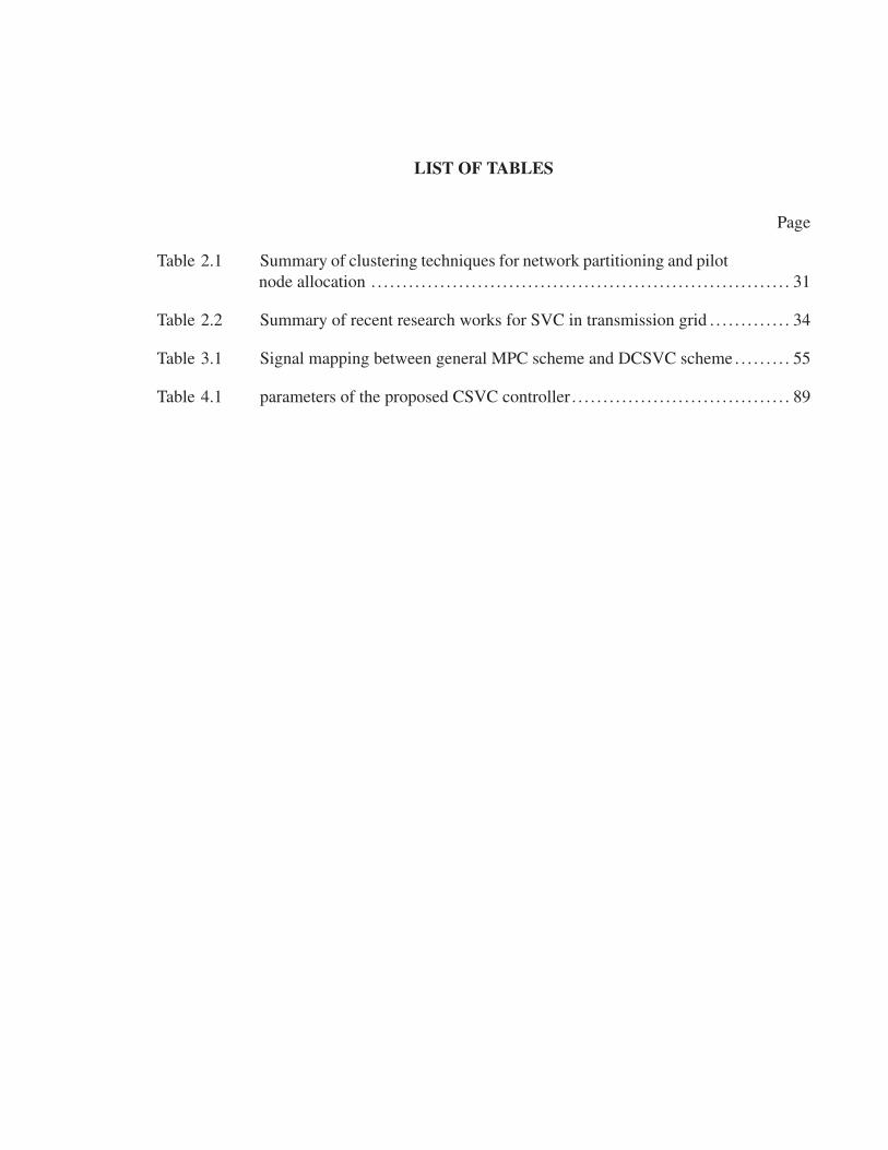
LIST OF TABLES
Page
Table 2.1 Summary of clustering techniques for network partitioning and pilot
node allocation . . . . . . . . . . . . . . . . . . . . . . . . . . . . . . . . . . . . . . . . . . . . . . . . . . . . . . . . . . . . . . . . . . . 31
Table 2.2 Summary of recent research works for SVC in transmission grid . . . . . . . . . . . . . 34
Table 3.1 Signal mapping between general MPC scheme and DCSVC scheme . . . . . . . . . 55
Table 4.1 parameters of the proposed CSVC controller . . . . . . . . . . . . . . . . . . . . . . . . . . . . . . . . . . . 89


LIST OF FIGURES
Page
Figure 1.1 Two bus system with generator at one side and a load on the other
side . . . . . . . . . . . . . . . . . . . . . . . . . . . . . . . . . . . . . . . . . . . . . . . . . . . . . . . . . . . . . . . . . . . . . . . . . . . . . . 12
Figure 1.2 Acceptable region satisfying Equation 1.7 . . . . . . . . . . . . . . . . . . . . . . . . . . . . . . . . . . . . 13
Figure 1.3 p− v curves for different values of tan(φ) . . . . . . . . . . . . . . . . . . . . . . . . . . . . . . . . . . . . . 16
Figure 1.4 p− v curve with load characteristic curves at two operating points
A & B . . . . . . . . . . . . . . . . . . . . . . . . . . . . . . . . . . . . . . . . . . . . . . . . . . . . . . . . . . . . . . . . . . . . . . . . . . . 17
Figure 1.5 Three bus system with transformer . . . . . . . . . . . . . . . . . . . . . . . . . . . . . . . . . . . . . . . . . . . . 18
Figure 1.6 The effect of different compensation devices on the PV curve . . . . . . . . . . . . . . . 19
Figure 1.7 Structure of secondary voltage controller, Corsi (2015) . . . . . . . . . . . . . . . . . . . . . . 23
Figure 2.1 Classification of SVC Control desing aspects . . . . . . . . . . . . . . . . . . . . . . . . . . . . . . . . . 32
Figure 2.2 Classification based on control methodologies . . . . . . . . . . . . . . . . . . . . . . . . . . . . . . . . 33
Figure 2.3 Classification based on type of compensator . . . . . . . . . . . . . . . . . . . . . . . . . . . . . . . . . . 35
Figure 2.4 Classification based on type of model used for control . . . . . . . . . . . . . . . . . . . . . . . 36
Figure 2.5 Classification based on type of network under control . . . . . . . . . . . . . . . . . . . . . . . . 37
Figure 2.6 Classification of SVC literature based on controller design
architecture . . . . . . . . . . . . . . . . . . . . . . . . . . . . . . . . . . . . . . . . . . . . . . . . . . . . . . . . . . . . . . . . . . . . . . 38
Figure 3.1 General MPC Scheme . . . . . . . . . . . . . . . . . . . . . . . . . . . . . . . . . . . . . . . . . . . . . . . . . . . . . . . . . . 53
Figure 3.2 DCSVC algorithm for multi-area power grid. . . . . . . . . . . . . . . . . . . . . . . . . . . . . . . . . . 54
Figure 3.3 Configuration of the real-time test-bench for validation of DCSVC
algorithm . . . . . . . . . . . . . . . . . . . . . . . . . . . . . . . . . . . . . . . . . . . . . . . . . . . . . . . . . . . . . . . . . . . . . . . . 58
Figure 3.4 High Voltage transmission network for 5000 bus power grid.
Larger circles represents selected pilot nodes. Different colors
represent different areas . . . . . . . . . . . . . . . . . . . . . . . . . . . . . . . . . . . . . . . . . . . . . . . . . . . . . . . . 59
Figure 3.5 Fitness value of identified models of network areas for
identification data . . . . . . . . . . . . . . . . . . . . . . . . . . . . . . . . . . . . . . . . . . . . . . . . . . . . . . . . . . . . . . . 61

XVIII
Figure 3.6 Scenario1-DCSVC (solid line) vs. No DCSVC (dashed line) cases . . . . . . . . . 62
Figure 3.7 Scenario2-DCSVC (solid line) vs. No DCSVC (dashed line) cases . . . . . . . . . 63
Figure 3.8 Scenario3-DCSVC (solid line) vs. No DCSVC (dashed line) cases . . . . . . . . . 65
Figure 4.1 Block diagram of the proposed controller . . . . . . . . . . . . . . . . . . . . . . . . . . . . . . . . . . . . . 78
Figure 4.2 Block diagram of the proposed controller . . . . . . . . . . . . . . . . . . . . . . . . . . . . . . . . . . . . . 82
Figure 4.3 IEEE 118-bus power network. Pilot nodes (solid rectangle) and
control bus (dashed rectangle) . . . . . . . . . . . . . . . . . . . . . . . . . . . . . . . . . . . . . . . . . . . . . . . . . 84
Figure 4.4 generating probability mass function for random
capacitor/inductor switching . . . . . . . . . . . . . . . . . . . . . . . . . . . . . . . . . . . . . . . . . . . . . . . . . . . 86
Figure 4.5 Algorithm for generating Input-Output data . . . . . . . . . . . . . . . . . . . . . . . . . . . . . . . . . . . 87
Figure 4.6 Error histogram for the identified NN sensitivity model of IEEE
118-bus test case . . . . . . . . . . . . . . . . . . . . . . . . . . . . . . . . . . . . . . . . . . . . . . . . . . . . . . . . . . . . . . . . 88
Figure 4.7 Scenario 1: Proposed method (solid line), Linear sensitivity based
CSVC (dotted line) and Traditional method (dashed line) . . . . . . . . . . . . . . . . . . . . 95
Figure 4.8 Scenario 1: Proposed method (solid line), Linear sensitivity based
CSVC (dotted line) & Traditional method (dashed line). . . . . . . . . . . . . . . . . . . . . . 96
Figure 4.9 Scenario 1: Proposed method (solid line), Linear sensitivity based
CSVC (dotted line) & Traditional method (dashed line). . . . . . . . . . . . . . . . . . . . . . 97
Figure 4.10 Scenario 2: Proposed method (solid line), Linear sensitivity based
CSVC (dotted line) and Traditional method (dashed line) . . . . . . . . . . . . . . . . . . . . 98
Figure 4.11 Scenario 2: Proposed method (solid line), Linear sensitivity based
CSVC (dotted line) & Traditional method (dashed line). . . . . . . . . . . . . . . . . . . . . . 99
Figure 4.12 Scenario 2: (Proposed method (solid line), Linear sensitivity based
CSVC (dotted line) & Traditional method (dashed line). . . . . . . . . . . . . . . . . . . . .100
Figure 4.13 Scenario 3: Proposed method (solid line), Linear sensitivity based
CSVC (dotted line) and Traditional method (dashed line) . . . . . . . . . . . . . . . . . . .101
Figure 4.14 Scenario 3: Proposed method (solid line), Linear sensitivity based
CSVC (dotted line) & Traditional method (dashed line). . . . . . . . . . . . . . . . . . . . .102

XIX
Figure 4.15 Evolution of the objective function at each time step of the
controller . . . . . . . . . . . . . . . . . . . . . . . . . . . . . . . . . . . . . . . . . . . . . . . . . . . . . . . . . . . . . . . . . . . . . . .103
Figure 5.1 A group of overlapping areas partitioned using modified sensitivity
analysis; pilot nodes (red nodes), shared buses (blue circles), nodes
with participant compensator (highlighted using green rectangles) . . . . . . . . .111
Figure 5.2 Secondary voltage control using neural network and SA . . . . . . . . . . . . . . . . . . . .113
Figure 5.3 Architecture of the proposed consensus strategy . . . . . . . . . . . . . . . . . . . . . . . . . . . . .115
Figure 5.4 Flowchart describing the interaction of SVC of Area i and the
consensus coordinator . . . . . . . . . . . . . . . . . . . . . . . . . . . . . . . . . . . . . . . . . . . . . . . . . . . . . . . . .123
Figure 5.5 Pareto-front curve of a two-objective optimization problem with its
linear estimation . . . . . . . . . . . . . . . . . . . . . . . . . . . . . . . . . . . . . . . . . . . . . . . . . . . . . . . . . . . . . . .124
Figure 5.6 IEEE 118-bus power network. Pilot nodes (solid rectangle) and
control bus (dashed rectangle) . . . . . . . . . . . . . . . . . . . . . . . . . . . . . . . . . . . . . . . . . . . . . . . .125
Figure 5.7 Configuration of the real-time test-bench for validation of DCSVC
algorithm . . . . . . . . . . . . . . . . . . . . . . . . . . . . . . . . . . . . . . . . . . . . . . . . . . . . . . . . . . . . . . . . . . . . . . .126
Figure 5.8 Scenario 1: Voltage error on the pilot buses. With consensus
strategy (solid line), without consensus strategy (dotted line) . . . . . . . . . . . . . . .127
Figure 5.9 Scenario 1: With consensus strategy (solid line), Without
consensus strategy (dotted line) . . . . . . . . . . . . . . . . . . . . . . . . . . . . . . . . . . . . . . . . . . . . . . .128
Figure 5.10 Scenario 2: Voltage error on the pilot buses. With consensus
strategy (solid line), without consensus strategy (dotted line) . . . . . . . . . . . . . . .129
Figure 5.11 Scenario 2: With consensus strategy (solid line), Without
consensus strategy (dotted line) . . . . . . . . . . . . . . . . . . . . . . . . . . . . . . . . . . . . . . . . . . . . . . .130


LIST OF ABREVIATIONS
AVR Automatic Voltage Regulator
CA Control Agent
CSVC Coordinated Secondary Voltage Control
DCSVC Decentralized Coordinated Secondary Voltage Control
DG ,Distributed Generations
DMPC Decentralised Model Predictive Control
DNP Distributed Network Protocol
EDF Electricite De France
EMTP-RV Electro-Magnetic Transient Program - Restructured Version
EXST IEEE Type ST1 Excitation System
FACTS Flexible Alternating Current Transmission System
FCM Fuzzy C-Means
GA Genetic Algorithm
GENROU Round Rotor Generator Model (Quadratic Saturation)
HCSD Hierarchical Clustering with Single electrical Distance
HCVS Hierarchical Clustering in Var control Space
HQ Hydro-Quebec
HV High Voltage
IP Integer Programming

XXII
IREQ Institute de Recherché d’Hydro-Quebéc
LTC Load Tap-Changers
LTI Linear Time Invariant
MIMO Multi-Input Multi-Output
MPC Model Predictive Control
MPCSVC Model Predictive Coordinated Secondary Voltage Controller
NLMPC Non-Linear Model Predictive Control
NN Neural Network
OEL Over Excitation Limiter
OLTC On Load Tap Changers
OPNET OPtimized Network Engineering Tools
PI Proportional-Integral
PMF Probability Mass Function
PMU Phasor Measurement Unit
PQ Load bus
PVC Primary Voltage Controller
QP Quadratic Programming
QR Reactive power Regulator
QSS Quasi Steady State
RVR Regional Voltage Regulator

XXIII
SA Simulated Annealing
SKC Spectral K-way Clustering
SM Synchronous Machine
SNR Signal to Noise Ratio
SPP Steam Power Plant
STAB Speed Sensitive Stabilizing Model
STATCOM STATic synchronous COMpensator
SVC Secondary Voltage Control
TGOV Steam Turbine-Governor
TSO Transmission System Operator
TVR Tertiary Voltage Controller
VAR Volt Ampere Reactive


INTRODUCTION
In nowadays power systems, higher utilization of transmission assets, increased distance be-
tween production sites and the load centers, delays in building new transmission projects, larger
interconnections and increased meshing, connection of large capacity units to higher voltage
levels have led the grid to work closer to its operational limits. In this situation, the auto-
matic control of grid’s voltage and reactive power becomes more critical and any inappropriate
strategy toward control of the grid may cause instabilities which could consequently lead to
cascading black-outs such as the one occurred in 2003 in North America.
On the other hand, in HQ transmission network, despite the existence of AVR on individual
generators or using FACTS devices, suitable voltage and VAR control solutions, capable of
maintaining reactive power supply and demand in presence of network contingencies while
considering higher loads and associated transmission losses, does not exist and the lack of real-
time and closed-loop automatic coordination of reactive power resources to improve voltage
profile in the grid is unjustifiably continuing.
To resolve these issues, hierarchical voltage control approach can be used in which voltage
control problem is broken into three levels hierarchically, with different considerations at each
level. In this hierarchy, the primary controllers are taking care of local voltage stability, while
the secondary level controller tries to control voltage of sensitive buses of the network, called
pilot nodes, by balancing of reactive power supply and demand over a control region. This
reactive power can be injected to the power system through generation level by means of gen-
erators or through transmission level by means of VAR compensation devices such as capacitor
banks, tap-changers & static var compensators. In the highest level of this hierarchy, there is
tertiary level controller which deals with the economic and security concerns of the overall
power system. These levels operate also in different timescales so that their actions do not
affect each other. While the primary controllers take action in few milliseconds, the secondary

2
level controllers update their control each few seconds and for the tertiary level it is in the order
of minutes.
This work is a part of research project with HQ. The thesis focuses on the secondary level
voltage control problem considering coordination between continuous and discrete type com-
pensators in one control area while taking into account the effect of the neighbor areas. In this
chapter, first, the problem statement and motivations of the research work are presented. The
objectives and the methodology of the thesis are discussed afterwards. It is then followed by
a section discussing the contributions of the thesis. Finally the organization of the thesis is
discussed.
0.1 Motivation and problem statement
In HQ’s transmission network, manual voltage control is still in use and it typically involves:
dispatching the generating units’ forecast reactive powers, scheduling the power plants’ high
side voltages, switching shunt capacitor or inductor banks for power factor correction and
voltage regulation, and setting the voltage set-points of LTC and FACTS controllers. This con-
ventional approach to solving the network voltage control problem is nowadays unsatisfactory
because dispatching units’ reactive power and scheduling plants’ high side voltages are based
on off-line forecasting and actual network operating conditions may be often quite different
from their forecast values. Moreover, voltage set-points coordination is often operated accord-
ing to written operator instructions or requested by the system operator when strongly needed:
untimely or inadequate control actions may occur during slow dynamic phenomena following
unexpected events.
To resolve these problems, HQ have planned to change the structure of its network from manu-
ally regulated to an hierarchical automated controlled structure so that the network can maintain
reactive power supply and demand automatically over the network. Such a control could be

3
done in generation level (by means of generators) and also in transmission level (static var
compensator, Capacitor/Inductor banks). Important issues that should be considered for such a
control strategy are as follows:
1. Optimal compensation of reactive power and voltage control considering compensators’
MVAR limits : one of the issues in CSVC is to compensate voltage deviation with minimum
reactive power injection/absorption by the compensators so that extra MVAR can be used
as a reserve for extreme system conditions. In addition, the control strategy should consider
the MVAR limits of each compensator and try to manage these reactive power resources
based on their limits;
2. For large disturbances, the operating point of the system on the p− v curve moves closer
to the critical point in which the behavior of the system is nonlinear. Therefore the method
should consider these nonlinearities;
3. Coordination of continuous type compensators (generators, static var compensators) and
discrete type compensators (capacitor banks, LTC) in an optimal way. For HQ network with
tens of compensators installed on transmission lines, considering both discrete and contin-
uous nature of these compensators along with nonlinear behavior of the system transforms
the control problem into an NP-hard problem which is challenging to be implemented in
real-time in one time step of the secondary voltage controller, i.e. few seconds. The strat-
egy toward CSVC should be so that it can be finally applicable in real-time for large scale
power grids;
4. Voltage control is naturally done using local controllers in an area where the distrubance has
occurred. In this regard using a centralized control strategy for a problem which is by nature
decentralized is not reasonable. Moreover a centralized approach is not computationally
beneficial since it has to solve a far more larger optimization problem. In this way, the
proposed method should have a decentralized architecture;

4
5. Despite decentralized architecture of the control approach, a secondary voltage controller
in one region should coordinate itself with the actions of the secondary voltage controller in
a neighbor area. An uncoordinated action between regional SVCs might lead to oscillatory
behavior in the two and finally lead to voltage collapse.
0.2 Objectives
0.2.1 General Objectives
The general objective of this research is to propose both centralized and decentralized coordi-
nated secondary voltage control strategy for a large scale transmission network which could be
implemented in real-time. The following issues should be considered:
1. Use the maximum capability of currently installed compensators without installing new
ones;
2. Apply secondary voltage control in an optimal way so that minimum reactive power is
injected into the power network and the remaining reactive power capacity can be preserved
for emergency conditions. Physical limits such as compensators’ MVAR limits should also
be considered in control approach;
3. Ensure coordination of continuous compensators (generators, static var compensators) and
discrete compensators (capacitor banks, LTC) in an optimal way;
4. Propose a decentralized strategy which fits well with nowadays multi-area power network
structure;
5. Consider interactions between areas and coordination between regional controllers.

5
0.2.2 Specific Objectives
1. Model identification of each area of multi area power system considering the nonlinearities
within the model;
2. Development of a real-time centralized optimization based control strategy to regulate volt-
age at pilot buses using only continuous type compensators;
3. Development of a real-time decentralized optimization based control strategy which con-
siders only continuous type compensators and takes into account the effect of the neighbor
areas in the control design;
4. Development of a real-time centralized optimization based control strategy to regulate volt-
age at pilot buses using both discrete and continuous type compensators;
5. Development of a real-time decentralized optimization based control strategy which takes
into account both continuous and discrete type compensators. It should also take into ac-
count the effect of the neighbor areas in control design;
6. Validation of the proposed control strategies on realistic power grids in real-time.
0.3 Methodology
Different methods are used and proposed throughout this thesis. In the following, the main
methodologies are categorized:
1. To address the specific objective 1, two different approaches are used to identify a model
which relates the inputs, i.e. action of the compensator devices, to the outputs, such as volt-
age magnitude on pilot buses, voltage on compensator buses and reactive power injection
by machines. In both methods, first a series of input-output data is generated. Then a model
is fitted to the data. The two approaches are as follows:
(a) Use sub-space method to identify a linear dynamical state-space model;
(b) Use neural network approach to fit a nonlinear static model to the input-output data.

6
2. To address specific objectives 2, centralized MPC method is used. This approach is based
on the linear dynamical state space model of the whole network obtained using method-
ology 1a. This model is then used to formulate a predictor function based on which an
optimization problem is established to minimize voltage error on pilot nodes using reactive
power injection by continuous type compensators;
3. To address specific objectives 3, decentralized MPC method is used. The difference be-
tween this method and methodology 2 is that for decentralized MPC a separate controller is
designed for each region of the grid. Also the interaction between neighbor areas are taken
into account by considering measured reactive power flowing through inter area tie-lines in
the identified model and defining it as measured disturbance;
4. To address specific objective 4, SA based optimization is used. This method is proposed to
solve mixed continuous-discrete type optimization problem. It can handle both discrete and
continuous type compensators considering nonlinear static model of the network mentioned
in methodology 1b;
5. To address specific objective 5, SA based optimization is used. The difference between
this method and methodology 4 is that for decentralized control strategy the coordination
between two neighbor regional controllers is done by a multi-agent solution in which the
secondary level controllers as well as the primary level controllers of some specific com-
pensators which have a considerable impact on the two regions come up with a consensus;
6. To address specific objective 6, the proposed methods are tested on different power system
test-cases such as IEEE 39 bus and 118 bus standard systems. These test cases include
the dynamics of the generators, excitation systems, turbine governors, power system stabi-
lizer’s as well as the effect of the over and under excitation limiters. To validate method-
ologies on more realistic and larger scale power grid, a 5000-bus power system is also been
used.

7
Moreover, to investigate the real-time performance of the proposed methodologies, the
model of the power systems are built inside ePHASORsim software which is a phasor
domain solver from Opal-RT Technology. These models are run on a real-time simulators
which is also provided by Opal-RT Technologies. These real-time simulation models also
take into account the effect of the communication channel to investigate the impact of the
communication noise and delay on the controller performance.
0.4 Contributions
Guided by the objectives presented in Section 0.2 and using the methodology proposed in
Section 0.3, this thesis presents the following important and novel contributions:
1. Proposing a novel nonlinear sensitivity model based on NN which maps reactive power
injection by compensators to the corresponding voltage variation on pilot nodes considering
different demand levels of the network;
2. Proposing a novel closed loop suboptimal secondary voltage controller which uses SA to
solve a mixed discrete-continuous type optimization problem with NN based sensitivity
model as nonlinear constraint and quadratic objective function at each time step of the
controller;
3. Proposing a novel technique to generate rich data for training Neural Network as the non-
linear sensitivity model;
4. Proposing a novel consensus strategy which does not require communication between re-
gional controllers;
5. Defining PVC of the shared compensators as an agent which communicates with neighbor
SVCs. This agent can then make a decision on its degree of participation on SVC control
of each neighbor area;

8
6. Proposing a modified version of sensitivity analysis presented in Corsi (2015) in which
control regions can overlap. Some compensators might be selected for SVC which belong
to the shared area;
7. Proposing a decentralized MPC approach in which the two neighboring MPCs does not
require any communication links between to coordinate their actions. Moreover, each re-
gional controller does not need to consider any model of its neighbors. The supplementary
information about neighboring areas are gathered from measuring tie-line reactive power
deviations using installed PMUs. In this way each regional controller considers the effect
of the other regions indirectly from this measurement;
8. Presenting a real-time simulation test-bed to validate the proposed methodologies in which
detailed dynamics of the network as well as standard communication protocols used to send
and receive the data in power systems are employed. The test-bench also benefits from the
multi-core simulation technologies on which the proposed decentralized controller is tested
and validated;
9. Using realistic test-cases with detailed dynamics to validate the controller. Such a valida-
tion has been missing in the literature where usually simplified academic test-cases such
as IEEE39 bus or IEEE118 bus networks are used for validation of the control algorithms.
Although using a smaller test-case can be considered at early stages of validation for con-
troller techniques, the final validation should be done on a more realistic data set to show
that the proposed methodologies are capable of handling complexity of large scale power
grids.
0.5 Publications
The contributions listed in Section 0.4 have been presented in three journals and two conference
publications. The complete list of publications associated with this research work is presented
below.

9
0.5.1 Journals
Published
[J1]: Morattab A., Akhrif O., Saad M., Decentralized Coordinated Secondary Voltage Controlof Multi-Area Power Grids using Model Predictive Control, Accepted for publication in
IET Generation, Transmission & Distribution; May 2017;
Submitted
[J2]: Morattab A., Saad M., Akhrif O., Lefebvre S., Dalal A., Nonlinear Sensitivity-based Co-ordinated Control of Reactive Resources in Power Grids Under Large Disturbances, sub-
mitted to International Journal of Electrical Power and Energy Systems; May 2018;
[J3]: Morattab A., Akhrif O., Saad M., Secondary Voltage Control with Consensus BetweenRegional Controllers, submitted to IEEE Transactions on Power Systems. February 2018;
0.5.2 Conferences
Published
[C1]: Morattab A., Dalal A., Akhrif O., Saad M., Lefebvre S., Model Predictive CoordinatedSecondary Voltage Control of Power Grids, 2012 International Conference on Renew-
able Energies for Developing Countries (REDEC), Pages: 1-6, November 2012, Beirut,
Lebanon;
[C2]: Morattab A., Saad M., Akhrif O., Dalal A., Lefebvre S., Decentralized coordinated sec-ondary voltage control of multi-area highly interconnected power grids, 2013 IEEE Pow-
erTech Conference, Pages: 1-5, June 2013, Grenoble, France.
0.6 Thesis Outline
The thesis is organized as follows: The next chapter reviews the fundamental concepts regard-
ing to voltage stability and control as well as secondary voltage control method. This chapter is
then followed by Chapter 2 which includes literature review related to our addressed problems.
Chapters 3-5 show the contribution of this research work.

10
Chapter 3 presents the first accepted journal paper (J1) corresponding to decentralized MPC
approach. This work is related to the first phase of this research work in which only the con-
tinuous type compensators are considered. Chapter 4 and chapter 5 present the second and
third papers (J2 and J3) respectively and they are related to the second phase of the research
work in which both continuous and discrete type compensators are considered. In chapter 4
the mixed discrete-continuous type optimization methodology based on NN model and SA op-
timizer is presented. However the control architecture is centralized. In chapter 5 the same
idea is adapted on a decentralized architecture in which a consensus strategy is also presented
to coordinated the decentralized controllers.
The thesis ends by conclusions that provide a summary of the addressed problems, the proposed
solutions and the future research works.
This thesis also includes two Appendices. In appendix I, the conference paper (C1) is presented
in which our early achievements on using centralized MPC is discussed. The idea presented
in this appendix was further extended in chapter 3. Moreover in appendix II, the second pub-
lished conference paper (C2) is presented which is an early evaluation of decentralized control
architecture and comparison to the centralized case.

CHAPTER 1
FUNDAMENTAL CONCEPTS
In this chapter, basic concepts regarding to voltage stability and control are first discussed.
Afterwards, classical secondary voltage control which was first presented in Arcidiacono et al.
(1977); Arcidiacono (1983) is reviewed. Finally the coordinated secondary voltage control,
presented first in Paul et al. (1987), is discussed.
1.1 Fundamentals of Voltage Stability and Voltage Control
1.1.1 Power flow, active and reactive power transfer limits
Consider the simple two bus network in Figure 1.1. An ideal voltage source with voltage E�0
supplies a remote load through a transmission line modeled as a series reactance. The receiving
end voltage V and angle θ depend on the active and reactive power transmitted through the line.
The power flow equation on the load bus can be written as follows:
S = P+ jQ = −(V∠θ)I∗ = −V∠θ(V∠θ −E
jX
)∗(1.1)
Expanding the right hand side of Equation 1.1 and finding its real and imaginary parts, active
and reactive power equations can then be written as Equations 1.2 and 1.3.
P = −EVX sin(θ) (1.2)
Q = EVX cos(θ)− V2
X(1.3)
After eliminating θ using the trigonometric identity we get:

12
Figure 1.1 Two bus system with generator
at one side and a load on the other side
(Q+ V2
X
)2+P2 =
(−EV
X
)2(1.4)
Solving for V2 yields:
V2 = E2
2 −QX ± X√
E4
4X2 −P2 −Q E2
X(1.5)
Thus, the problem has real positive solutions if:
P2+Q E2
X ≤ E4
4X2 (1.6)
This inequality shows which combinations of active and reactive power line can supply to the
load. Substituting the short-circuit power at the receiving end, Ssc =E2
X , we get:
P2+QSsc −( Ssc2 )2 ≤ 0 (1.7)
The locus of all (P,Q) pairs satisfying Equation 1.7 is shown in Figure 1.2, underneath the
parabola curve representing the case where the left side of 1.7 is equal to zero. As can be seen
the parabola is symmetric with respect to the Q axis. Moreover, the active power transfer limits
when Q = 0 are defined as − Ssc2 as lower and Ssc
2 as higher limit. On the other hand, the reactive
power has only a maximum transfer limit when P = 0 and it is equal to Ssc4 .

13
Figure 1.2 Acceptable region satisfying Equation 1.7
Observing Figure 1.2, the following could be deduced:
1. An injection of reactive power at the load end, i.e. reducing Q, increases the transfer limit
for active power;
2. Both active and reactive power transfer limits are proportional to the short circuit power,
Ssc. Based on the definition of Ssc, one can also say that increasing the line admittance, X ,
reduces the transfer limits while increasing the voltage on the generation bus, E , increases
these limits;
3. The transfer of positive reactive power through the inductive line is limited to Ssc4 . How-
ever, any amount of active power can be transferred through the line by injecting enough

14
inductive load on the load side. This fact confirms that transfer of reactive power is more
difficult than active power over the inductive lines.
1.1.2 PV curve, voltage stability and voltage control
For simplicity, we assume that the load shown earlier in Figure 1.1 is a constant impedance
type. Mathematically:
P+ jQ = V2G(1+ j tan(φ)) (1.8)
With this assumption, one can say that the load produces reactive power for leading power
(tan(φ) < 0) and absorbs reactive power for lagging power (tan(φ) > 0). Now we convert the
variables to their per unit (p.u.) equivalent, assuming Ssc as the base power and E as the base
voltage:
p =P
Ssc(1.9a)
q =QSsc
(1.9b)
v =VE
(1.9c)
g =G1X
(1.9d)
Using per unit quantities, the positive solution to Equation 1.5 can be written as:
v =1√
g2+ (1+g tan(φ))2(1.10)

15
We also have the following equations for p and q:
p = v2g (1.11a)
q = v2g tanφ (1.11b)
For a constant tan(φ), one can plot a parametric curve of per unit voltage versus per unit active
power, called p− v curve, based on Equation 1.10 and Equation 1.11a for different values of
parameter g changing from 0 to infinity, Figure 1.3 shows the p-v curves for different values of
tan(φ).
The green area shown in Figure 1.3 is defined as voltage controlled region in which the voltage
magnitude is within 5%p.u. of tolerance from the 1p.u.. Moreover, for a constant tan(φ),
the nose of each curve, marked using star, defines the maximum active power transfer. The
corresponding voltage is often referred to as the critical voltage. Connecting the nose of the
curves together forms a new curve, called critical curve, which divides the p− v plane into
stable and unstable regions in which the unstable region is shown as shaded area.
To clarify the concept of voltage stability, Figure 1.4 illustrates the p− v curve, shown in blue,
considering tan(φ) = 0. As can be seen in this figure, for a specific load value two different
operating points, shown as A and B, exist. The load characteristic curve, defined in Equa-
tion 1.11a, is also shown in green for each operating point. As can be seen in this figure, at
point A, by increasing the load by ΔP, the operating point changes to a new one A’ which
has a lower voltage magnitude. However, the load has a tendency to decrease p when voltage
decreases. This represents a stable fixed-point at operating point A which leads the system to
return back to its original equilibrium point, A. On the other hand, at point B which is located
underneath of the nose of the curve, the load characteristic curve along with the p− v curve
forms an unstable fixed-point which causes a divergent pattern of perturbed point B’ from the
original point B.

16
Figure 1.3 p− v curves for different values of tan(φ)
The same conclusion can be made for other operating points on the p− v curve, hence it could
be divided into stable and unstable regions as depicted in Figure 1.3.
1.1.3 Effect of different compensation devices
In normal conditions of a power system, voltage magnitude is mostly affected by reactive power
injection. For the simple two bus network of Figure 1.1, this could be seen by calculating the
derivatives, ∂P∂V and ∂Q∂V , based on Equations 1.2 and 1.3. These derivatives are shown below:

17
Figure 1.4 p− v curve with load characteristic curves at two operating points A & B
∂P∂V = −
EX sin(θ) (1.12)
∂Q∂V =
EX cos(θ)− 2V
X(1.13)
Since in normal conditions θ ≈ 0, then sin(θ) ≈ 0 and cos(θ) ≈ 1. In this way, ∂P∂V ≈ 0 and
∂Q∂V ≈ E
X − 2VX . This result confirms the decoupling of voltage magnitude and active power in
normal conditions. The same conclusion could be made about decoupling of voltage angle and
reactive power. These two facts are the basic assumptions which are considered in decoupled

18
power flow algorithm and shows that in practice, it is reasonable to control voltage magnitude
by reactive power and voltage angle by active power injection/absorption.
Various reactive power compensation devices are used throughout a power grid to control volt-
age locally. However, they can be categorized into two main groups which are continuous type
and discrete type compensators. Continuous type compensators are devices which are able to
deliver any continuous value of reactive power within their operational limits. Synchronous
generators, synchronous condensers and FACTS devices are examples of this type of compen-
sators. On the other hand, discrete type compensators are switch base devices which can only
deliver discrete amounts of reactive power to the grid. Capacitor banks, inductor banks and tap
changers are considered as discrete type compensators.
To show the effect of different compensation devices, Figure 1.5 illustrates a three-bus power
system with one generator bus connected to the neighbor bus through an inductive transmission
line with a capacitor in series. This bus is then connected to the load bus with a tap changer. A
shunt capacitor and a shunt inductor are also connected to the load bus. Moreover, Figure 1.6
shows the p− v curve for the load bus and the effect of these reactive power compensation
devices as well as the terminal voltage of the generator on this curve. As can be seen in this
figure, these elements can be considered as control actuators to change the system stiffness,
critical voltage and the theoretical and practical transfer limits so that the voltage remains in
the acceptable bound considering any disturbances on the network.
Figure 1.5 Three bus system with transformer

19
a) Shunt capacitor, shunt inductor, fixed
reactive power injection
b) Increase reference voltage of generator,
series capacitor, tap ratio
Figure 1.6 The effect of different compensation devices on the PV curve
1.2 Secondary Voltage Control
Secondary voltage control consists of two main steps. The first step is to partition the transmis-
sion system into several voltage coherent regions and finding a representative bus, called pilot
bus, for each area. The participant reactive power compensators for each region which control
the voltage of the pilot node in that region are also allocated in this step. The second step is
then to design the secondary level control loop which calculates the control signals based on
the measurements from the pilot nodes and sends them to the primary level controllers, which
control the compensation devices. These two steps are discussed in this section.
1.2.1 Network partitioning and pilot node selection in SVC
In this section, the method presented in Corsi (2015) to find pilot nodes and partitioning the
network is presented. This method is based on sensitivity analysis and the criterion to choose
is based on the weakest buses to the reactive power disturbances.
Suppose a power system with n buses, N of which are PQ buses and g are generator buses
(PV and slack buses). We assume that pilot buses are always a subset of PQ buses. Sensitivity

20
matrix, Svq, as defined in Equation 1.14 relates reactive power injection on each PQ bus to the
voltage variation of all PQ buses.
Svq =
⎡⎢⎢⎢⎢⎢⎢⎢⎢⎢⎢⎢⎢⎣
∂V1∂Q1
∂V1∂Q2
· · ·∂V1∂QN
∂V2∂Q1
∂V2∂Q2
· · ·∂V2∂QN
....... . .
...
∂VN
∂Q1
∂VN
∂Q2· · ·
∂VN
∂QN
⎤⎥⎥⎥⎥⎥⎥⎥⎥⎥⎥⎥⎥⎦(1.14)
The procedure toward finding pilot buses is as follows:
1. Matrix Svq rows and columns are reordered to satisfy the condition:
⎧⎪⎪⎨⎪⎪⎩(Svq
) (1)11 <
(Svq
) (1)rr(
Svq) (1)11 >
(Svq
) (1)21 >
(Svq
) (1)31 > · · · >
(Svq
) (1)N1
with r = 2, · · · ,N .
2. The "electrical distance" ratios are computed as follows:
βi j =(Svq)
(1)i j
(Svq)(1)j j
with i = 1,2, · · · ,N and j = 1,2, · · · , Z . It should be noted that 0 ≤ βi j < 1 and Z is the num-
ber of pilot nodes, to be defined at the end.
3. After the lower limit of the electrical distance among the pilot nodes is established, we
exclude from subsequent selections those buses related to the first N1 rows of the S(1)vq re-
ordered matrix having coupling coefficient βi1 with bus “1” greater than εp, i.e.:
εp <(Svq)
(1)μ1
(Svq)(1)11
≤ 1; μ = 1, · · · ,N1.

21
4. The remaining (N − N1) = n1 columns of the S(1)vq matrix are reordered in such a way that
the new matrix S(2)vq satisfies the following inequalities:
⎧⎪⎪⎨⎪⎪⎩(Svq
) (2)11 <
(Svq
) (2)rr(
Svq) (2)11 >
(Svq
) (2)21 >
(Svq
) (2)31 > · · · >
(Svq
) (2)N1
where S(2)vq ∈ Rn1×n1 and r = 2, · · · ,n1. This corresponds to arranging the (n−N1) remaining
buses in order of electrical vicinity, with bus 1, among them, having the highest power.
5. Similar to step 3, in the steps that follow we no longer consider the first N2 of the n1 nodes
(that is, the first N2 rows of the reordered matrix S(2)vq having coupling coefficient with bus
“1”:
εp <(Svq)
(2)μ1
(Svq)(2)11
≤ 1; μ = 1, · · · ,N2.
6. The reordering procedure of the matrices is repeated, starting from the (n1 − N2) = n2 re-
maining nodes, in accordance with the indicated procedure up to the (Z + 1)th reordering,
which is when among the (nZ−1 − NZ ) = nZ remaining buses, the coefficient S(Z+1)vq of the
reordered matrix S(Z+1)vq is greater than a predefined value 1
γ , which represents the minimum
admissible value of the short circuit power for a pilot node:
(Svq)(Z+1)11 >
1γ.
7. The Z pilot nodes are those corresponding to the first row of the matrices: S(1)vq ,S
(2)vq ,S
(3)vq , · · · ,
S(Z)vq .
8. After having defined the pilot nodes, the buses belonging to each region are classified using
the electrical distance values calculated at step 2. In this way, the ith bus is linked to area
j if it has the highest coupling coefficient with the jth pilot node. That is, the ith bus is
associated to area j if:
βi j > βik .∀k � j .

22
1.2.2 SVC Control structure
Although the voltage of local buses to which reactive power compensator devices are con-
nected are regulated, voltages of other buses might deviate from their desired values due to
load variations or contingencies. In this way, besides their local control responsibilities, these
compensators should also contribute to the long term voltage/reactive power stability and con-
trol. Such a regional control should be done in a way that takes into account the limitation of
each compensator and its droop characteristics. For this reason SVC has been introduced by
Arcidiacono et al. (1977); Arcidiacono (1983) and Paul et al. (1987). Based on this method
the network is first partitioned into theoretically non-interacting zones, within which, voltage
is controlled independently. SVC adjusts automatically the reactive power of certain generat-
ing units to control the voltage at a specific point, known as the pilot nodes, considered as the
representative bus of the zone.
The structure of SVC is shown in Figure 1.7. The SVC system measures the instantaneous
voltage of the pilot bus of the zone Vp, compares it with the voltage set-point Vre fp , generated
by TVR level, and applies a PI law using RVR to determine a signal representing the reactive
power required for this zone, q. The RVR control law is defined as Equation 1.15.
q = KPV
(Vre f
p −Vp
)+KV I
∫ t0
(Vre f
p −Vp
)dt
with :
qmax ≤ q ≤ qmin
(1.15)
qmax and qmin are normalized upper and lower limits of the RVR which are equal to -1 and +1.
The normalized power is then converted to its actual level using Qre f = qQlim.
Qre f is then used by local QRs at reactive power sources, to control their reactive power output
with respect to their own reserves by modulating the input of the corresponding AVR.

23
Figure 1.7 Structure of secondary voltage controller, Corsi (2015)
ΔVre f = KIQ∫ t0(Qre f −Qg
)dt
with :
Vmax ≤ V ≤ Vmin
(1.16)
Despite the advantages of SVC, the following limitations are pointed out in Lefebvre et al.
(2000):

24
1. In some regions, coupling between theoretically independent zones has increased as a result
of grid development subsequent to implementation of SVC. To avoid instability, we must
therefore correct the number of zones or accept degradation in control dynamics;
2. SVC requires reactive-power alignment of the generating units involved, but makes no al-
lowance for excessive demand that might be made on certain units as a result of differences
in physical proximity;
3. The internal reactive-power control loop at generating-unit level is a destabilizing factor
that can actually amplify the initial disturbance in the first few instants following certain
incidents (generator dropout, for example);
4. The system makes only partial allowance for operating constraints. For example, it does not
fully integrate monitoring of permissible voltage limits or generating set operating limits;
5. Control loop parameters are fixed, which precludes optimum allowance for operating con-
ditions;
6. The signal representing the required reactive power level varies at a rate that makes no
allowance for generating unit response capabilities.
Due to the limitations above, Paul et al. (1987); Lefebvre et al. (2000) presented Coordinated
SVC which is discussed in the following.
1.3 Coordinated Secondary Voltage Control
The original method for CSVC is based on optimization which has been first introduced by
EDF Paul et al. (1987) for French integrated power network. The cost function to be minimized
is defined as follows:
minΔU
[λV ‖α (VC −VP)−CVΔU‖2
+λq��α (Qre f −Q
)−CqΔU
��2
+ λu��α (Ure f −U
)−ΔU
��2] (1.17)
and it is subject to the following constraints:

25
|ΔU | ≤ ΔUmax
VminTHT ≤ VTHT +CVΔU ≤ Vmax
THT
α(Q+CqΔU
)+ bΔU ≤ c
(1.18)
where α is the control gain, U & ΔU are respectively terminal voltage reference of generators
and its deviation, Vp and VTHT are voltage at pilot buses and voltage at high voltage side of
the generators respectively, VC is set-point values at pilot points and Qre f and Ure f are set-
point values for reactive power generation and for terminal voltage. Moreover, CV and Cq
are sensitivity matrices linking terminal voltage variation to pilot node voltage variation and
generators’ reactive power variation respectively. Mathematically:
ΔVp = CVΔU
ΔQ = CqΔU(1.19)
Unlike classical SVC which is based on PI control law, the optimization problem formulated in
Equations 1.17 to 1.19 is a MIMO control problem which considers a linearized model of the
system and takes into account all of the constraints when solving for the terminal voltage of the
generators within one region. In this way, many pilot nodes could be controlled simultaneously
by coordinating many generators in a region considering physical limitations.


CHAPTER 2
LITERATURE REVIEW
2.1 Introduction
In this chapter, a thorough review of the literature regarding to secondary voltage control is
presented. In this regard, a brief history of different implementations of this method around the
world is discussed. Afterwards a systematic approach is used to classify all related works in
this domain. The classification is based on different considerations regarding to SVC problem
which have been taken into account in the research work. The works are finally presented in
tables.
2.2 Literature Review
The origins of wide area voltage and reactive power control could be traced back to reactive
power dispatch problem in which the reactive power resources are allocated throughout the
network to minimize power loss while maintaining voltage of the buses within desired limits.
However this approach is based on the study of off-line forecasting while actual network oper-
ating conditions are often different from forecasted values and therefore unpredictable. In this
way, some works at early 70s have considered real-time voltage/reactive power control, namely
Hano et al. (1969); Nakamura & Okada (1969); Narita & Hammam (1971a,b) have proposed
a centralized and decentralized real-time two stage optimization method which first minimizes
voltage deviation using conjugate gradient method and second minimizes reactive power loss
over transmission lines using direct search technique. In this work both continuous and discrete
value compensators are considered, however discrete values are calculated by round off. The
method was successfully implemented by Kyushu Electric Power Company in Japan.
Although the works presented earlier propose the partitioning of the transmission system for
regional voltage control, the concept of hierarchical voltage control as well as classical sec-
ondary voltage control methodology are explicitly proposed in Arcidiacono et al. (1977);

28
Happ & Wirgau (1978); Arcidiacono (1983); Paul et al. (1987). In this method, the power
network is divided into many theoretically non-interacting zones and at each zone, the most
sensitive bus to reactive power disturbances is selected as pilot node. Voltage at this bus is then
measured and compared with a desired voltage dictated by tertiary level controller. Regional
controller, which is basically a PI controller calculates the total amount of reactive power that
is needed to compensate the voltage deviation and sends this signal to the regional participant
generators. At generation level, a reactive power control loop, which is also a PI controller,
calculates the new voltage set-point for the AVR, considering the generator’s participation fac-
tor as well as its reactive power limits. The proposed method was successfully implemented in
Italian and French Power grids.
As has been discussed further in Lefebvre et al. (2000); Vu et al. (1996), the assumption of
one sensitive bus per control zone may not be realistic for a densely meshed network, such as
French transmission grid. For these networks, they have proposed CSVC algorithm, which is
basically an optimal, model based, multi-input/multi-output, regional controller. CSVC uses
voltage measurements from many sensitive buses in a control zone and calculates new set-
points for generators that take part in secondary voltage control loop considering their reactive
power and voltage limits. CSVC utilizes a linear sensitivity model which relates voltage mag-
nitude to reactive power injection for all PQ buses in the grid. It also uses another sensitivity
matrix which relates voltage at PV buses to voltage at PQ buses of the grid. Recalculation of
these sensitivity matrices are triggered by an event or an incident (change of topology, unit
tripping, major load change). Further details on the advantages of model based CSVC com-
pared to the method presented in Arcidiacono et al. (1977); Arcidiacono (1983), can be found
in Lefebvre et al. (2000); Vu et al. (1996).
Another approach regarding to the SVC is proposed by Ilic-Spong et al. (1988) which combines
pilot bus selection and voltage control together to find minimal number of pilot nodes which
are able to maintain voltage at the desired reference as well as the control gain. This method
solves a mixed integer nonlinear program using SA.

29
The works presented so far have paved the way for hierarchical voltage control to be imple-
mented in different countries around the world. A comprehensive review of different imple-
mentations of SVC in different countries can be found in Martins & Corsi (2007) and Corsi
(2015).
Triggered by the above major works, a lot of effort has been made in academic domain also
to improve these methods or to present alternative approaches. Each of these manuscripts
investigate different aspects of SVC problem and take into account different considerations.
However, by investigating these works, some common features are extracted and are used to
classify the literature regarding to the SVC control design problem.
In the following, relative research works are summarized in two sections. In Section 2.3,
research works related to Network partitioning, pilot bus selection and compensator allocation
are reviewed. Afterwards, in Section 2.4 a general classification map is extracted based on the
different aspects of secondary voltage control problem. An analysis of the current literature
is presented and based on the drawbacks of the recent works the objectives of the proposed
research are justified.
2.3 Network partitioning and pilot node selection
One of the earliest methods for pilot bus selection and network partitioning is presented in
Corsi (2015) and applied in Italian network. The method is based on short-circuit capacities
and sensitivity analysis of the network. In this approach, the buses are sorted from the most to
the least sensitive one. Afterwards the least sensitive buses are selected as pilot nodes based on
an iterative process. The number of pilot buses are dependent on two predefined parameters.
The first parameter, 1γ , defines the minimum admissible threshold value of the short circuit
power for a pilot node. Any bus with short circuit power smaller than this threshold will not
be considered as a pilot bus. The second parameter is called coupling coefficient threshold, εp,
which defines the minimum admissible limit for coupling of remote buses to a pilot bus. Any

30
remote bus with coupling value smaller than εp will not be considered in the same control area
as the pilot bus.
Another major work regarding to pilot bus selection is presented in Ilic-Spong et al. (1988), in
which a minimal number of pilot nodes are allocated using SA method to control the voltage in
the network. In this approach pilot node selection and feedback gain design are mixed together
and are done simultaneously. Conejo et al. (1994) compares different optimization algorithms
to solve the same problem stated in Ilic-Spong et al. (1988). Also Sancha et al. (1995, 1996)
and Amraee et al. (2012, 2010) have proposed different versions of the same method as Ilic-
Spong et al. (1988).
Another category of network partitioning and pilot node selection is based on clustering methods.
La Gatta et al. (2014) & Alimisis & Taylor (2015) have surveyed these methods thoroughly.
In general, network partitioning based on clustering includes two steps: 1) A zoning algorithm
which breaks the network into areas appropriate for SVC control and 2) A pilot node selection
algorithm that identifies a representative bus of the zone for voltage control.
Clustering techniques to partition power grid are usually composed of three parts as below:
1. A proximity measure: An “electrical distance” that represents the degree of similarity for
any two nodes;
2. A clustering criterion: A cost function or some other type of rule to form a number of zones
utilizing the proximity measure;
3. Optimal number of clusters: A way to assess the appropriate number of clusters.
Table 2.1 summarizes the methods presented in the literature for network partitioning and pilot
node selection.

31
Table 2.1 Summary of clustering techniques for network
partitioning and pilot node allocation
Method Paper Proximity mea-sure
Clustering crite-rion
Optimal No. ofcluster
HCSD Lagonotte
et al.(1989)
Logarithm of the
product of ratios
of elements in vqsensitivity matrix
Agglomerative
clustering (bot-
tom to top) using
complete linkage
criterion
Where relative
diameter for two
consecutive no.
of clusters are
maximum
HCVS Sun et al.(2013)
Euclidean norm
of difference
between vq sen-
sitivity elements
of two node
Agglomerative
clustering (bot-
tom to top) using
average linkage
criterion
Where average
inter-cluster
distance is maxi-
mum
SKC Mehrjerdi
et al.(2013b)
Normalized
laplacian.
Weights of
adjacency matrix
are the same as
electrical dis-
tance defined in
HCSD
Change of cen-
troid points are
below threshold
Given
FCM Mehrjerdi
et al.(2013a)
Same as HCSD Weighted dis-
tance from cen-
troid is smaller
than a threshold.
Weights are
defined as fuzzy
membership
functions.
Given
2.4 Classification of SVC control design literature based on different aspects
Figure 2.1 shows a general scheme of different aspects of any SVC problem. Moreover Fig-
ures 2.2 to 2.6 illustrate each of these aspects in detail and classify the literature for each one
which is sorted in a chronological order.

32
SVCControlDesignAspects
Controlmethodology
PI control law Optimizationbased control
MPC
Fuzzy controlOther methods
Controlarchitecture
Centralized
Decentralized Without consid-ering the impactof neighbor area
Consideringthe impact ofneighbor area
Distributed(Decentralized
with consensus)
Type ofmodel usedfor control
Static Lin-ear modelStatic Non-
linear model
DynamicLinear model
Dynamic Non-linear model
Type ofcompensatorused for SVC
Continuous
Discrete
Discrete &continuous Type of
networkunder control
Transmission
Distribution
Microgrid
Figure 2.1 Classification of SVC Control desing aspects
2.4.1 Analysis of the literature
The analysis of the literature in this section follows the following assumptions:

33
Controlmethodology
PI control law
Optimizationbased control
MPCFuzzy control
OtherMethods
•Arcidiacono et al. (1977)
•Arcidiacono (1983)
•Paul et al. (1987)
•Flórez et al. (1994)
•Richardot et al. (2006)
•Da Silva et al. (2013)
•Shafiee et al. (2014c)
•Shafiee et al. (2014b)
•Shafiee et al. (2014a)
•Simpson-Porco et al.(2015)
•Lu et al. (2016)
•Hamidi et al. (2016)
•Lai et al. (2016)
•Schiffer et al. (2016)
•Guo et al. (2016)
•Yu et al. (2016)
•Hano et al. (1969)
•Narita & Hammam
(1971a)
•Narita & Hammam
(1971b)
•Happ & Wirgau (1978)
•Ertem & Tudor (1987)
•Vu et al. (1996)
•Marinescu & Bourles
(1999)
•Lefebvre et al. (2000)
•Vaccaro et al. (2011)
•Mehrjerdi et al. (2013d)
•Amadou et al. (2014)
•Trakas et al. (2014)
•Alimisis & Taylor (2015)
•Mezquita et al. (2015)
•Yang et al. (2016)
•Larsson et al. (2002)
•Zima & Andersson (2003)
•Larsson & Karlsson
(2003)
•Wen et al. (2004)
•Hiskens & Gong (2006)
•Negenborn (2007)
•Beccuti et al. (2010)
•Jin et al. (2010)
•Glavic et al. (2011)
•Ma et al. (2013)
•Moradzadeh et al. (2013)
•Ma & Hill (2014a)
•Ma & Hill (2014b)
•Ma & Hill (2017)
•Larsson (1999)
•Wang et al. (2003)
•Ruey-Hsun & Yung-Shuen
(2003)
•Mehrjerdi et al. (2013b)
•Loia et al. (2013)
•Bernard et al. (1996)
•Wang (2001)
•Dragosavac et al. (2012)
•Mehrjerdi et al. (2013c)
•Bottura & Borghetti
(2014)
•Cai et al. (2016)
•Li et al. (2016)
•Su et al. (2016)
•Chen et al. (2016)
•Borghetti et al. (2017)
Figure 2.2 Classification based on control methodologies
• Due to the focus of this research work on the SVC in transmission system, only literatures
implementing SVC in transmission grid are considered;
• To limit the scope of the analysis to recent literature, only works published from 2010 are
considered.
Considering the above assumptions, the literature is narrowed down to Table 2.2.
In Beccuti et al. (2010) the SVC problem is formulated in a centralized way. However the
optimization problem is decomposed using Lagrangian decomposition. In this way only local
measurements are employed to achieve global optima.

34
Table 2.2 Summary of recent research works for SVC in transmission grid
Reference ControlMethod
Type ofModel
Control Architecture Type ofcompen-sator
Beccuti et al.(2010)
MPC Linear, Dy-
namic
Centralized Continuous
Jin et al.(2010)
MPC Linear, Dy-
namic
Centralized Continuous
& Discrete
Glavic et al.(2011)
MPC Nonlinear,
Static
Centralized Continuous
& Discrete
Dragosavac
et al. (2012)
Feedback
gain
Linear,
Static
Centralized Continuous
Mehrjerdi
et al. (2013b)
Fuzzy con-
trol
Nonlinear,
Static
Decentralized, considers the effect
of neighbor areas, no consensus
Continuous
Ma et al.(2013)
MPC,
multi-
objective
Nonlinear,
Dynamic,
adaptive
Centralized Continuous
& Discrete
Moradzadeh
et al. (2013)
MPC Nonlinear,
Dynamic
Decentralized, considers the effect
of neighbor areas, no consensus
Continuous
& Discrete
Da Silva et al.(2013)
PID control Linear,
Static
Decentralized, no consideration
neighbor areas, no consensus
Continuous
Mehrjerdi
et al. (2013d)
Optimization Nonlinear,
Static
Decentralized, considers the effect
of neighbor areas, no consensus
Continuous
Mehrjerdi
et al. (2013c)
Neural Net-
work
Nonlinear,
Static
Decentralized, considers the effect
of neighbor areas, no consensus
Continuous
Ma & Hill
(2014a)
MPC,
multi-
objective
Nonlinear,
Dynamic
Centralized Discrete
Ma & Hill
(2014b)
MPC,
multi-
objective
Nonlinear,
Dynamic
Centralized Discrete
Amadou et al.(2014)
Optimization Linear,
Static
Decentralized, no consideration
neighbor areas, no consensus
Continuous
Trakas et al.(2014)
Optimization Nonlinear,
Static,
Probabilis-
tic
Decentralized, considers the effect
of neighbor areas, no consensus
Continuous
Mezquita et al.(2015)
Optimization Nonlinear,
Static
Centralized Continuous
Su et al.(2016)
Successive
Minimiza-
tion
Nonlinear,
Static
Centralized Continuous

35
Type ofcompensator
Continuous
Discrete
Both con-tinuous &
discrete
•Paul et al. (1987)
• Ilic-Spong et al. (1988)
•Conejo et al. (1994)
•Sancha et al. (1995)
•Vu et al. (1996)
•Sancha et al. (1996)
•Conejo & Aguilar (1998)
•Marinescu & Bourles
(1999)
•Lefebvre et al. (2000)
•Wang (2001)
•Wang et al. (2003)
•Richardot et al. (2006)
•Hiskens & Gong (2006)
•Beccuti et al. (2010)
•Jin et al. (2010)
•Dragosavac et al. (2012)
•Mehrjerdi et al. (2013b)
•Loia et al. (2013)
•Da Silva et al. (2013)
•Mehrjerdi et al. (2013d)
•Mehrjerdi et al. (2013c)
•Bottura & Borghetti
(2014)
•Shafiee et al. (2014c)
•Shafiee et al. (2014b)
•Shafiee et al. (2014a)
•Amadou et al. (2014)
•Trakas et al. (2014)
•Simpson-Porco et al.(2015)
•Mezquita et al. (2015)
•Lu et al. (2016)
•Cai et al. (2016)
•Li et al. (2016)
•Yang et al. (2016)
•Hamidi et al. (2016)
•Lai et al. (2016)
•Schiffer et al. (2016)
•Guo et al. (2016)
•Yu et al. (2016)
•Su et al. (2016)
•Chen et al. (2016)
•Borghetti et al. (2017)
•Bernard et al. (1996)
•Larsson (1999)
•Larsson et al. (2002)
•Larsson & Karlsson
(2003)
•Ruey-Hsun & Yung-Shuen
(2003)
•Ma & Hill (2014a)
•Ma & Hill (2014b)
•Ma & Hill (2017)
•Hano et al. (1969)
•Narita & Hammam
(1971a)
•Narita & Hammam
(1971b)
•Flórez et al. (1994)
•Zima & Andersson (2003)
•Wen et al. (2004)
•Negenborn (2007)
•Vaccaro et al. (2011)
•Glavic et al. (2011)
•Ma et al. (2013)
•Moradzadeh et al. (2013)
Figure 2.3 Classification based on type of compensator
In Jin et al. (2010) a real-time protection and security scheme is presented with centralized
MPC in its core. Voltage stability margins are also considered as constraints inside optimization
problem. The optimization problem is formulated as QP and then the calculated continuous
values are discretized.
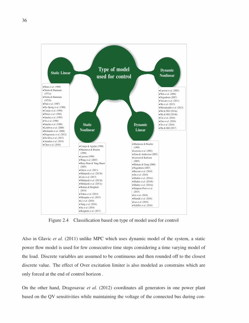
36
Type of modelused for control
Static Linear
StaticNonlinear
DynamicLinear
DynamicNonlinear
•Hano et al. (1969)
•Narita & Hammam
(1971a)
•Narita & Hammam
(1971b)
•Paul et al. (1987)
• Ilic-Spong et al. (1988)
•Conejo et al. (1994)
•Flórez et al. (1994)
•Sancha et al. (1995)
•Vu et al. (1996)
•Sancha et al. (1996)
•Lefebvre et al. (2000)
•Richardot et al. (2006)
•Dragosavac et al. (2012)
•Da Silva et al. (2013)
•Amadou et al. (2014)
•Chen et al. (2016)•Conejo & Aguilar (1998)
•Marinescu & Bourles
(1999)
•Larsson (1999)
•Wang et al. (2003)
•Ruey-Hsun & Yung-Shuen
(2003)
•Glavic et al. (2011)
•Mehrjerdi et al. (2013b)
•Loia et al. (2013)
•Mehrjerdi et al. (2013d)
•Mehrjerdi et al. (2013c)
•Bottura & Borghetti
(2014)
•Trakas et al. (2014)
•Mezquita et al. (2015)
•Li et al. (2016)
•Yang et al. (2016)
•Su et al. (2016)
•Borghetti et al. (2017)
•Marinescu & Bourles
(1999)
•Larsson et al. (2002)
•Zima & Andersson (2003)
•Larsson & Karlsson
(2003)
•Hiskens & Gong (2006)
•Negenborn (2007)
•Beccuti et al. (2010)
•Jin et al. (2010)
•Shafiee et al. (2014c)
•Shafiee et al. (2014b)
•Shafiee et al. (2014a)
•Simpson-Porco et al.(2015)
•Lu et al. (2016)
•Hamidi et al. (2016)
•Lai et al. (2016)
•Schiffer et al. (2016)
•Larsson et al. (2002)
•Wen et al. (2004)
•Negenborn (2007)
•Vaccaro et al. (2011)
•Ma et al. (2013)
•Moradzadeh et al. (2013)
•Ma & Hill (2014a)
•Ma & Hill (2014b)
•Cai et al. (2016)
•Guo et al. (2016)
•Yu et al. (2016)
•Ma & Hill (2017)
Figure 2.4 Classification based on type of model used for control
Also in Glavic et al. (2011) unlike MPC which uses dynamic model of the system, a static
power flow model is used for few consecutive time steps considering a time varying model of
the load. Discrete variables are assumed to be continuous and then rounded off to the closest
discrete value. The effect of Over excitation limiter is also modeled as constrains which are
only forced at the end of control horizon .
On the other hand, Dragosavac et al. (2012) coordinates all generators in one power plant
based on the QV sensitivities while maintaining the voltage of the connected bus during con-

37
Type of networkunder control
Transmission
Distribution
Microgrid
•Hano et al. (1969)
•Narita & Hammam
(1971a)
•Narita & Hammam
(1971b)
•Paul et al. (1987)
• Ilic-Spong et al. (1988)
•Conejo et al. (1994)
•Flórez et al. (1994)
•Sancha et al. (1995)
•Vu et al. (1996)
•Bernard et al. (1996)
•Sancha et al. (1996)
•Conejo & Aguilar (1998)
•Marinescu & Bourles
(1999)
•Lefebvre et al. (2000)
•Wang (2001)
•Larsson et al. (2002)
•Wang et al. (2003)
•Zima & Andersson (2003)
•Larsson & Karlsson
(2003)
•Wen et al. (2004)
•Hiskens & Gong (2006)
•Negenborn (2007)
•Beccuti et al. (2010)
•Jin et al. (2010)
•Glavic et al. (2011)
•Dragosavac et al. (2012)
•Mehrjerdi et al. (2013b)
•Ma et al. (2013)
•Moradzadeh et al. (2013)
•Da Silva et al. (2013)
•Mehrjerdi et al. (2013d)
•Mehrjerdi et al. (2013c)
•Ma & Hill (2014a)
•Ma & Hill (2014b)
•Amadou et al. (2014)
•Trakas et al. (2014)
•Mezquita et al. (2015)
•Su et al. (2016)
•Ma & Hill (2017)
•Larsson (1999)
•Larsson et al. (2002)
•Zima & Andersson (2003)
•Ruey-Hsun & Yung-Shuen
(2003)
•Richardot et al. (2006)
•Vaccaro et al. (2011)
•Loia et al. (2013)
•Bottura & Borghetti
(2014)
•Borghetti et al. (2017)
•Shafiee et al. (2014c)
•Shafiee et al. (2014b)
•Shafiee et al. (2014a)
•Simpson-Porco et al.(2015)
•Lu et al. (2016)
•Cai et al. (2016)
•Li et al. (2016)
•Yang et al. (2016)
•Hamidi et al. (2016)
•Lai et al. (2016)
•Schiffer et al. (2016)
•Guo et al. (2016)
•Yu et al. (2016)
•Chen et al. (2016)
Figure 2.5 Classification based on type of network under control
tingencies. The control is done in two steps: 1-Voltage controller which relates the voltage of
power plant bus bar (high side) to the total required reactive power. 2-Reactive power con-
troller which defines the share of each generator for the compensation. Outputs are defined as
reference voltage variations.

38
Controlarchitecture
Centralized
DecentralizedWithout
consideringthe impactof neighbor
area
Consideringthe impactof neighbor
area
Distributed(Decentral-ized with
consensus)
•Hano et al. (1969)
•Narita & Hammam
(1971a)
•Narita & Hammam
(1971b)
• Ilic-Spong et al. (1988)
•Conejo et al. (1994)
•Conejo & Aguilar (1998)
•Larsson (1999)
•Larsson et al. (2002)
•Zima & Andersson (2003)
•Larsson & Karlsson
(2003)
•Ruey-Hsun & Yung-Shuen
(2003)
•Wen et al. (2004)
•Richardot et al. (2006)
•Hiskens & Gong (2006)
•Beccuti et al. (2010)
•Jin et al. (2010)
•Glavic et al. (2011)
•Dragosavac et al. (2012)
•Ma et al. (2013)
•Ma & Hill (2014a)
•Ma & Hill (2014b)
•Mezquita et al. (2015)
•Yang et al. (2016)
•Su et al. (2016)
•Ma & Hill (2017)
•Arcidiacono et al. (1977)
•Arcidiacono (1983)
•Paul et al. (1987)
•Flórez et al. (1994)
•Vu et al. (1996)
•Lefebvre et al. (2000)
•Da Silva et al. (2013)
•Mehrjerdi et al. (2013c)
•Amadou et al. (2014)
•Marinescu & Bourles
(1999)
•Mehrjerdi et al. (2013b)
•Moradzadeh et al. (2013)
•Mehrjerdi et al. (2013d)
•Trakas et al. (2014)
•Sancha et al. (1995)
•Sancha et al. (1996)
•Wang (2001)
•Wang et al. (2003)
•Negenborn (2007)
•Vaccaro et al. (2011)
•Loia et al. (2013)
•Bottura & Borghetti
(2014)
•Shafiee et al. (2014c)
•Shafiee et al. (2014b)
•Shafiee et al. (2014a)
•Simpson-Porco et al.(2015)
•Lu et al. (2016)
•Cai et al. (2016)
•Li et al. (2016)
•Hamidi et al. (2016)
•Lai et al. (2016)
•Schiffer et al. (2016)
•Guo et al. (2016)
•Yu et al. (2016)
•Chen et al. (2016)
•Borghetti et al. (2017)
Figure 2.6 Classification of SVC literature based on controller design architecture
Mehrjerdi et al. (2013b) present a K-way partitioning method to divide the Laplacian graph of
the network. Then pilots are selected as most sensitive buses through applying different levels
of disturbance to each region. Finally, a fuzzy controller is designed for each region which
considered the effect of the neighbors by measuring tie-line reactive power.

39
Also in Ma et al. (2013) a multi-objective optimization method is formulated and solved using
GA. First objective is to maintain voltage at reference while the second one is to minimize the
switching steps of the compensators. At each run, the solution is saved in a knowledge based
memory which will be used later in the initial population of the GA when similar situation
occurs.
Moreover, Moradzadeh et al. (2013) propose a nonlinear hybrid model as a model of the system
which includes the model of OLTC and OEL. Greedy method is used to solve combinatorial
optimization problem for each area. The planned local value is communicated to the neighbor
areas for their next time step.
In Da Silva et al. (2013), a classical SVR using PI control law is presented. The novelty is to
add joint line droop compensation to the control loop.
In Mehrjerdi et al. (2013d), coordination between regional controllers is studied. A connection
matrix is defined which represent the connection between regional controllers and also between
the controllers of the neighbor areas. Based on this matrix, the regions which have connection
between their controllers are aggregated and the optimization is solved for the aggregated net-
work.
Also in Mehrjerdi et al. (2013c) the model of each region is identified using Neural Network.
From this model then a reverse model is identified as the controller who is also a neural net-
work.
In addition, in Ma & Hill (2014a) same approach as Ma et al. (2013) with more details and
discussion on how to create an off-line data base of knowledge. How the controller works.
And how the knowledge is integrated to the controller. Then Ma & Hill (2014b) discuss the
adaptive feature of the controller in details.
In Amadou et al. (2014), first the compensators clusters are identified using agglomerative hier-
archical algorithm. The proximity of the nodes which is based on the normalized susceptance
matrix is used as the criterion. Second the load buses are classified and the pilot nodes are

40
selected using method presented in Arcidiacono et al. (1977). For control, method presented
in Paul et al. (1987) is used.
Also in Trakas et al. (2014) particle swarm optimization is used to solve probabilistic optimiza-
tion problem to find optimal voltage reference of generators as well as reactive power injection
by capacitors. Voltage of the boundary buses are also kept constant to avoid the interference of
the areas on each other.
Moreover Mezquita et al. (2015) propose a self organizing map to partition the network based
on the electrical distance metric. For pilot bus selection, method presented in Ilic-Spong et al.
(1988) is used. For control, optimal power flow is used. Calculated continuous shunt values
are finally discretized to the closest discrete value.
Finally in Su et al. (2016), a successive linearization of nonlinear function is used to solve
nonlinear optimization problem in which the objective function is defined as the infinity norm
of voltage error.
Analysing the methods above, the following drawbacks are observed:
1. In Jin et al. (2010); Glavic et al. (2011); Mezquita et al. (2015) the optimization problem is
originally solved as a continuous type problem and the value for discrete type compensators
are then approximated by rounding off continuous values. Although this assumption is
computationally beneficial, neglecting the round-off error especially when the discrete steps
are large, may lead to oscillatory behavior when the problem is solved for consecutive time
steps;
2. The method presented in Ma et al. (2013); Ma & Hill (2014a,b) is a centralized approach
which has only considered discrete type compensator. The algorithm lacks considering
the continuous type compensators. Moreover due to the local nature of the voltage con-
trol problem there is no need to apply a centralized approach which is computationally
inefficient;

41
3. Decentralized methods presented in Mehrjerdi et al. (2013b); Moradzadeh et al. (2013);
Da Silva et al. (2013); Mehrjerdi et al. (2013d,c); Amadou et al. (2014); Trakas et al.
(2014) have not considered any consensus between regional controllers. In this regard,
action of some compensators in one region might have impacts on the voltage of the pilot
bus for a neighbor region which is not seen by the SVC of the neighbor region. In some
cases, such an uncoordinated strategy between regional controllers may lead to oscillatory
behaviors and voltage collapse;
4. Validation of the methods is limited to off-line simulations while only small test-cases such
as IEEE 39 and 118 bus system are considered. Although the methods are proved to be
operational for such test-cases, their operation might face challenges which comes to a
large scale power system, hence they should be evaluated for such realistic test-cases.
2.5 Conclusion
Based on the analysis of the literature review done in Section 2.4.1, the need for a decentral-
ized SVC method which considers the nonlinearities of the system and takes into account both
continuous and discrete type compensator in the optimization problem while considering con-
sensus between regional controllers is felt. This is inline with the objectives and methodologies
of this research work which are presented in sections 0.2 and 0.3 respectively.


CHAPTER 3
DECENTRALIZED COORDINATED SECONDARY VOLTAGE CONTROL OFMULTI-AREA POWER GRIDS USING MODEL PREDICTIVE CONTROL
Arvin Morattab1, Ouassima Akhrif1, Maarouf Saad1
1 Department of Electrical Engineering, École de Technologie Supérieure,
1100 Notre-Dame Ouest, Montréal, Québec, Canada, H3C 1K3
Paper published in IET Generation, Transmission & Distribution, May 2017
Abstract
This manuscript presents a decentralized control scheme for CSVC of large-scale power net-
works. In this way, for each area of the power grid, an MPC which modifies the set-points of
reactive power compensators participating in CSVC algorithm is designed. The proposed con-
troller takes into account reactive power limits of these compensation devices. The novelty of
the method lies in the consideration of measured reactive power deviation on tie-lines between
neighboring areas as measured disturbance and compensation of the disturbance by regional
MPC controllers. As another contribution of this work, the validation of the proposed algo-
rithm is done in real-time simulation environment in which the decentralized MPC controllers
are run in parallel on separate computational cores. The stability and robustness of the pre-
sented algorithm is validated for a large scale realistic transmission network with 5000 buses
considering standard communication protocols to send and receive the data. Simulation results
show that the proposed method can regulate the voltages on the pilot buses at the desired values
in presence of load variations and communication delays. Finally, the computational burden of
the proposed method is evaluated in real-time.
Introduction
One of the well-known strategies toward voltage control in large-scale multi-area power net-
works is to use a hierarchical control structure. In this method, the controller consists of three

44
levels in which the lowest level, i.e. primary controller, tries to maintain transient voltage stabil-
ity at local buses, while the secondary level controller works regionally to maintain long-term
voltage stability by balancing reactive power supply and demand through injection/absorption
of reactive power into/from the network. The latter is done by controlling the voltage of some
sensitive load buses (PQ buses) of each area, called pilot nodes. The reactive power needed for
such control can be either injected/absorbed by generators or using VAR compensation devices
such as capacitor/inductor banks, static var compensator and FACTS. Finally, at the highest
level of the hierarchical controller, i.e. tertiary level, economic and security concerns of the
overall power system are maintained. The operation of different levels of this hierarchical
controller is divided geographically and temporally so that they have minimum interference
between each other. In this way, the primary, secondary and tertiary level controllers react
in few seconds, few minutes and up to 15 minutes while they operate locally, regionally and
nationally.
A lot of research has been done regarding hierarchical secondary voltage control since its intro-
duction by EDF in 1985 Paul et al. (1987). This research covers many aspects of such strategy
including division of the large-scale power network into electrically distant areas (Mehrjerdi
et al. (2013b); Kamwa et al. (2009); Tuglie et al. (2008)), selection of the pilot buses (Mehrjerdi
et al. (2013b); Conejo & Aguilar (1998); Lerm (2006); Amraee et al. (2012)), locating the re-
active power compensators over the network (Ghahremani & Kamwa (2013); Pretelt (1971);
Mendoza et al. (2007); Happ & Wirgau (1978); Ertem & Tudor (1987)) as well as controller
design techniques (Vu et al. (1996); Lefebvre et al. (2000); Richardot et al. (2006); Sancha
et al. (1995); Wang (2001); Wang et al. (2003); Larsson (1999); Larsson et al. (2002); Fenichel
(1979); Juang & Pappa (1985); Moore (1981); Marinescu & Bourles (1999); Zima & Anders-
son (2003); Larsson & Karlsson (2003); Wen et al. (2004); Hiskens & Gong (2006); Beccuti
et al. (2010)). Since the contributions of this manuscript are mostly related to control design
technique and its validation, the following literature review is mainly focused on this aspect of
the works.

45
Regarding controller design techniques, these researches mostly consider CSVC of reactive
compensators in transmission and distribution networks, as well as the interaction between
neighbor areas and the impact of DG. In this way, Vu et al. (1996); Lefebvre et al. (2000)
have applied a centralized multivariable optimal control strategy for meshed power grids to
minimize voltage deviations at pilot buses considering generators reactive power limits, gen-
erator buses and pilot buses voltage limits. Moreover, sensitivity matrices have been used to
describe input-output relations of the network. The static optimization approach discussed in
Paul et al. (1987) has been used in Richardot et al. (2006) considering DGs effect in CSVC
algorithm. Also Sancha et al. (1995) has proposed a decentralization of the same approach for
CSVC of multi area power systems. In Larsson et al. (2002), a predictive control with tree
search optimization method is applied to coordinate capacitor banks and tap-changers. More-
over Wang (2001); Wang et al. (2003); Larsson (1999); Fenichel (1979) apply different fuzzy
control techniques for CSVC problem. In this regard, Wang (2001) and Wang et al. (2003)
have proposed a multi-agent, fuzzy based control method for coordination of AVRs, SVCs and
STATCOM in the case of power system contingencies. Moreover Larsson (1999) has used a
fuzzy rule based controller to coordinate cascade tap-changers in radial distribution feeders. In
addition, Fenichel (1979) utilizes a set of information collected by modal analysis to formulate
a two stage fuzzy logic-based model, considering voltage variation on load buses and reactive
power reserve of compensators as input, and also generator’s reference voltage as output.
The control methods discussed so far have designed secondary voltage controllers assuming
post-contingency stability of the network, i.e the transient response of the system is assumed
to vanish after few seconds and the network reaches its new steady state due to the operation
of the primary level controllers. In this way, a static model of the system can be used for
secondary level controllers. Although this assumption is computationally beneficial, there are
certain slow dynamics in the network which might result in voltage instability and eventually
voltage collapse when the system is working close to its limits or faces harsh disturbances such
as change of topology, unit tripping and major load changes. A solution to this problem is to
46
use MPC method in which a real-time optimization problem is solved at each time step of the
controller based on a pre-identified dynamic model of the power network.
Considering MPC applications in secondary voltage control, Marinescu & Bourles (1999) has
proposed an MPC based algorithm using both static and dynamic optimization methods. In
Zima & Andersson (2003), MPC has been used for emergency voltage control and the model
is defined based on sensitivity analysis of network’s dynamic model. Larsson & Karlsson
(2003) has applied tree search optimization techniques inside MPC algorithm to coordinate
generators, tap changers as well as load shedding in extreme conditions. In Wen et al. (2004),
the nonlinear model of the grid has been used as the model for MPC and Euler state prediction
and pseudo gradient evolutionary programming is used to develop the coordinated controller.
In Hiskens & Gong (2006), MPC method is used to determine minimum amount of load shed-
ding to restore system voltages. Beccuti et al. (2010) has considered both coordination of
generators and load shedding using MPC and the optimization is formulated as a centralized
quadratic programming via Lagrangian decomposition. In Jin et al. (2010), shunt capacitors
are switched based on control commands generated by MPC to prevent voltage collapse and
to maintain a desired stability margin after a contingency. Also Glavic et al. (2011) has used
a multi-step optimization method for MPC controller to improve voltage profile in transmis-
sion network and to prevent long-term voltage instability. Finally, Moradzadeh et al. (2013)
has applied MPC algorithm in a distributed way for CSVC of multi-area power systems. In
this method, a communication line is established between CAs designed for each area so that
regional controllers take into account decisions made by their neighboring areas’ optimization
algorithm.
In recent years, the growing trend toward smart grids with integration of DERs has led to a
major shift in researches regarding to voltage control. These works have mostly focused on
the application of adaptive cooperative multi-agent control techniques in transmission & dis-
tribution Vaccaro et al. (2011); Loia et al. (2013); Ma et al. (2013); Ma & Hill (2014a,b); Bot-
tura & Borghetti (2014); Su et al. (2016); Borghetti et al. (2017) as well as micro-grids Shafiee
et al. (2014c,b,a); Simpson-Porco et al. (2015); Lu et al. (2016); Cai et al. (2016); Li et al.

47
(2016); Yang et al. (2016); Hamidi et al. (2016); Lai et al. (2016); Schiffer et al. (2016); Guo
et al. (2016); Yu et al. (2016); Ma & Hill (2017).
Focusing on the works on transmission & distribution, Vaccaro et al. (2011) proposes a decen-
tralized non-hierarchical voltage regulation architecture in which the states regarding to the dy-
namics of the neighbor areas are synchronized to the weighted average of the variables sensed
by all the controllers in the smart grid. Moreover, Loia et al. (2013) proposes decentralized
and non-hierarchal voltage control architecture based on cooperative fuzzy agents to achieve
consensus. Also Ma et al. (2013); Ma & Hill (2014a,b) propose an adaptive centralized CSVC
method in which a multi-objective optimization problem is solved using GA to find pareto-
optimal solution, i.e. switching of OLTC & capacitor banks. In addition Bottura & Borghetti
(2014); Borghetti et al. (2017) discusses an asynchronous leaderless multi agent approach that
coordinates the reactive power compensators. This paper also presents a simulation test-bench
in which an electro-mechanical transient program, EMTP-rv, is interfaced with a communi-
cation network simulator, OPNET, to validate the performance of the proposed algorithm as
well as the effects of communication network latency and packet loss. Finally, Su et al. (2016)
formulates CSVC as a nonlinear successive ∞-norm minimization problem in which the load
disturbances are estimated on-line.
This study proposes a DCSVC approach using MPC method for Multiple TSO power grids.
It is assumed that control areas are selected in a way that there are minimum interferences
between regional MPCs. Hence, unlike Vaccaro et al. (2011), no communication links are
established between regional controllers and the DCSVC of each area does not need to know
any quasi-state space model of the neighbors. However, the supplementary information on
inter-area disturbances is obtained by measuring tie-line reactive power deviations using in-
stalled PMU. It is also shown that the proposed method can be implemented on large scale
transmission systems such as the 5000 bus power network used in this study.
Another contribution of this work is to propose a real-time test bench to test and validate wide
area control algorithms such as the proposed DCSVC. Unlike Bottura & Borghetti (2014);

48
Borghetti et al. (2017), the proposed test-bench operates in real-time. This test-bench is also
flexible to apply any control strategy, either for voltage or frequency, and using centralized,
decentralized, or distributed control architectures. In case of decentralized and distributed
topologies, a dedicated computational core can be assigned to each regional controller, hence
making it suitable for performance evaluation of such control strategies.
The real-time test-bench is implemented using OPAL-RT’s Real-time simulator, having ePHA-
SORsim as its main phasor domain solver Jalili-Marandi et al. (2013),Opal-RT (2018). ePHA-
SORsim is designed for real-time simulation of transient stability phenomena for large-scale
transmission and distribution power systems. In contrast to off-line simulation tools such as
PSS/e..., the real-time performance of ePHASORsim makes it a suitable tool to play as a back-
bone simulation engine to test, validate, and tune local and wide area control and protection
schemes. The controller and power system can run on separate platforms and link together
through Ethernet based protocols (such as DNP, C37.118 , etc.).
The rest of this paper is organized as follows: Section 3.1 discusses the principle of the pro-
posed decentralized MPC algorithm and its application to CSVC problem. Section 3.2 presents
the proposed real-time test-bench for decentralized architecture of DCSVC in which computa-
tions regarding to regional controllers are done in parallel cores while the phasor domain dy-
namic model of the power network is run on a separate one. Section 3.3 presents the DCSVC
procedure applied on a large power system with 5000 buses in three steps: First step includes
pilot bus selection, controllers’ allocation and network partitioning using sensitivity analysis
described in Corsi (2015). Following, system identification procedure toward finding linear
dynamical equivalent of each area of partitioned network suitable for MPC algorithm is dis-
cussed. The model is identified considering voltages at pilot buses as measured outputs and
set-points of compensation devices as control inputs. Moreover generated reactive power by
these compensators are defined as unmeasured outputs. These estimated outputs are used by
MPC to respect the reactive power limits imposed by physical limitations. Real-time evalua-
tion of DCSVC algorithm on this network shows its scalability to be implemented on realistic
large-scale power grids. Finally, Section 3.4 concludes the paper and discusses future works.

49
3.1 Decentralized Model Predictive Coordinated Secondary Voltage Control
3.1.1 Model Predictive Control formulation
Consider that the dynamic behavior of a system is approximated by LTI state space model as
follows:
x(k +1) = Ax(k)+Buu(k)+Bvv(k)+ d(k)
ym(k) = Cmx(k)+Dvmv(k)
yu(k) = Cux(k)+Dvuv(k)
(3.1)
Where x(k) is the nx-dimensional state vector of the system, u(k) is the nu-dimensional vector
of control inputs, v(k) is the nv-dimensional vector of measured disturbances, d(k) is the nd-
dimensional vector of unmeasured disturbances entering the system, ym(k) is the vector of
measured outputs, and yu(k) is the vector of unmeasured outputs. The overall ny-dimensional
output vector y(k) combines both ym(k) and yu(k), i.e. y(k) = [ym(k), yu(k)]t .
Figure 3.1 illustrates a general scheme of MPC controller. As can be seen, the controller
consists of three main blocks which are Estimation, Prediction and optimization. The LTI
model of Equation 3.1 is used by the estimation and prediction blocks to estimate the state
vector and then to predict future outputs. By employing these two steps, the dynamics of the
system are translated to constraints of an optimization problem in which the only unknown is a
vector of successive control variables increments in a finite horizon, called control horizon. At
time k the procedure toward finding the optimal control input, u∗(k), is described as follows:
3.1.1.1 State estimation
The estimator is a Kalman filter which estimates the state vector, x(k), knowing previous es-
timated state x(k − 1), measured output ym (k), measured disturbance v (k) and also previous
value of control input, u∗ (k −1) in presence of the unmeasured disturbance, d (k). the unmea-

50
sured disturbance is generally defined as the output of a linear disturbance model for which the
input is considered to be a white noise with a known covariance matrix.
3.1.1.2 Prediction
The estimated state is then used by the predictor to define the p-step ahead outputs of the
system, y(k + i |k) i = 1, · · · , p, as a linear function of future control input increments. In
this formulation, p is called prediction horizon. Reference Camacho & Alba (2013) derives
predictor equations as shown in Equation 3.2 & Equation 3.3.
⎡⎢⎢⎢⎢⎢⎢⎢⎢⎢⎢⎣
y(k +1|k)
y(k +2|k)...
y(k + p|k)
⎤⎥⎥⎥⎥⎥⎥⎥⎥⎥⎥⎦= Sx x(k)+ Su∗u∗(k −1)+ Su
⎡⎢⎢⎢⎢⎢⎢⎢⎢⎢⎢⎣
Δu(k)
Δu(k +1)...
Δu(k + p)
⎤⎥⎥⎥⎥⎥⎥⎥⎥⎥⎥⎦+ Sv
⎡⎢⎢⎢⎢⎢⎢⎢⎢⎢⎢⎣
v(k)
v(k +1)...
v(k + p)
⎤⎥⎥⎥⎥⎥⎥⎥⎥⎥⎥⎦(3.2)
in which:

51
Sx =
⎡⎢⎢⎢⎢⎢⎢⎢⎢⎢⎢⎣
CA
CA2
...
CAp
⎤⎥⎥⎥⎥⎥⎥⎥⎥⎥⎥⎦,Su∗ =
⎡⎢⎢⎢⎢⎢⎢⎢⎢⎢⎢⎣
CBu Du 0 . . . 0
CABu CBu Du . . . 0...
......
. . ....
CAp−1Bu CAp−2Bu CAp−3Bu . . . Du
⎤⎥⎥⎥⎥⎥⎥⎥⎥⎥⎥⎦
Sv =
⎡⎢⎢⎢⎢⎢⎢⎢⎢⎢⎢⎣
CBv Dv 0 . . . 0
CABv CBv Dv . . . 0...
......
. . ....
CAp−1Bv CAp−2Bv CAp−3Bv . . . Dv
⎤⎥⎥⎥⎥⎥⎥⎥⎥⎥⎥⎦
Su =
⎡⎢⎢⎢⎢⎢⎢⎢⎢⎢⎢⎢⎣
Du +CBu Du 0 . . . 0
Du +CBu +CABu Du +CBu Du . . . 0...
...... . . .
...
Du +p∑
i=1CAp−i Bu Du +
p∑i=2
CAp−i Bu Du +p∑
i=3CAp−i Bu . . . Du +CBu
⎤⎥⎥⎥⎥⎥⎥⎥⎥⎥⎥⎥⎦
(3.3)
In this formulation, the control input increment is defined as Δu(k + i) = u(k + i) − u(k). For
simplicity, we also assume that v(k+i)= v(k) for i = 1, . . ., p. In this way, the dynamic behavior
of the system for duration of [k, k + p] is translated to a set of linear equations in which the only
unknowns are control input increments, Δu(k + i) for i = 0, . . ., p.
3.1.1.3 Optimization
The optimizer then calculates this unknown control sequence by solving an optimization prob-
lem which minimizes the quadratic objective function in Equation 3.4 subject to the system
constraints. Different QP techniques exist in the literature to solve the optimization prob-
lem of Equation 3.4. A comprehensive review of existing QP methods is presented in Cama-
cho & Alba (2013). In this paper, the method presented in Schmid & Biegler (1994) is used.

52
minΔu(k),···,u(k+p−1)
p∑j=1Δy (k + j)t QΔy (k + j)+
Δu (k + j)t RΔu (k + j)
Δy (k + j) = (ym (k + j)− r (k))
s.t :
1)Equations 3.2 & 3.3
2)ymin < y (k + j) < ymax
3)umin < u (k + j) < umax
4)Δumin < Δu (k + j) < Δumax
(3.4)
Beside constraints forced by the predictor, umax and umin define maximum and minimum limits
of control inputs and Δumax and Δumin define maximum and minimum limits on control input
increments. Moreover, limits on output vectors are defined by ymax and ymin.
In order to deal with the computational burden of optimal controller, the degrees of freedom of
the optimization problem (number of unknown variables) can usually be reduced by consider-
ing constant control inputs after several time-steps, i.e. Δu (k + j) = 0 for j =m, · · · , p. in which
m is defined to be the control horizon. By this assumption, the optimization problem defined
by Equation 3.4 can be solved by available methods for quadratic optimization problems. Con-
sidering [Δu∗ (k), · · · ,Δu∗ (k +m−1)] as the optimal control solution, the first element of this
vector, Δu∗ (k), is finally used to find the control input using u∗ (k) = u∗ (k −1)+Δu∗ (k) which
will be applied on the real system. The whole procedure will be repeated in the next sampling
time with the prediction frame moving one sampling interval forward.

53
Figure 3.1 General MPC Scheme
In the following, a decentralized version of the MPC method is adopted for large-scale power
system’s secondary voltage control application.
3.1.2 Proposed DCSVC scheme
Figure 3.2 illustrates a typical three-area power network with their corresponding DCSVC
controller. The proposed approach can be generalized to any continuous type reactive power
compensator, however in Figure 3.2, we have used exciters connected to synchronous ma-
chines, shown as SM in, and SVCs to describe the proposed method. In this figure, Vi jPN is
the voltage at jth pilot node in Area i which should be maintained close to its desired value,
Vi jPNd , defined by tertiary level controller. This control is done by voltage for jth exciter or
SVC participating in the DCSVC of Area i, Vi jre f . Furthermore, the interaction of neighboring

54
areas is represented by the reactive power transferred through ni j different tie-lines between
Area j to Area i defined by Qi jltie in which l = 1, · · · ,ni j . The tie line vector is then defined as
Qi jtie =
[Qi j1
tie , · · · ,Qi jni jtie
]which is measured on mutual buses of tie-lines. The values of Vi j
PN
and Qi jtie are measured by DCSVCi and then the control input Vi j
re f is calculated. The objective
here is to apply the MPC Algorithm as a DCSVC to each area of multi-area power network in
Figure 3.2. The challenges are how to define the model, objective function and constraints in
Equation 3.4 for DCSVC problem. For this reason, the inputs and outputs of the system for
DCSVC problem based on general MPC scheme in Section 3.1.1, are presented in Table 3.1.
Figure 3.2 DCSVC algorithm for multi-area power grid
According to this table, the state space model for Area i is defined as follows:

55
Table 3.1 Signal mapping between general MPC scheme and DCSVC scheme
Signal in GeneralMPC Scheme
Corresponding Signal for DCSVC model
Reference Input r(k) Desired Voltage at pilot buses Vi jPNd(k)
Control Input u(k) Changes of reference voltage of compensator
devices Vi jre f (k)
Measured disturbance
Input v(k)Tie-line reactive power Qi j
tie(k)
Unmeasured distur-
bance Input d(k)Load changes, faults, un-modeled dynamics,
. . .
Measured Output ym(k) Pilot bus voltage Vi jPN (k)
Unmeasured Output
yu(k)Injected reactive power by Compensators (syn-
chronous machines and static var compensators,
...) Qi jCOMP(k)
xi(k +1) = Ai xi(k)+BiuVi
re f (k)+BivQ
itie(k)+ d(k)
ViPN (k) = Ci
mxi(k)+DivmQi
tie(k)
QiCOMP(k) = Ci
uxi(k)+DivuQi
tie(k)
(3.5)
In which xi is the state vector for Area i, Vire f =
[Vi1
re f ,Vi2re f , · · · ,V
inire f
] tis the control input vector
which includes reference voltages of ni compensators in Area i, Qitie is measured disturbance
vector Qitie =
[Qi1
tie,Qi2tie, · · · ,Q
iritie
] twhich is reactive power of tie-lines between Area i and all
other ri neighbor areas , ViPN =
[Vi1
PN,Vi2PN, · · · ,V
iNi
PN
] tis measured output vector which includes
voltage on Ni pilot buses and finally QiCOMP =
[Qi1
COMP,Qi2COMP, · · · ,Q
iciCOMP
] tis unmeasured
output vector representing reactive power injected by synchronous machines and SVCs.
Ai, Biu, Bi
v, Cim, Ci
u, Divm and Di
vu are matrices regarding to the identified state space LTI model
for each area.
In this way, the optimization problem for DCSVC can be formulated as Equation 3.6:

56
minΔV i
re f
p−1∑j=0
[ΔVi
re f (k + j)t RΔVire f (k + j)
+ΔViPN (k)t QΔVi
PN (k)]
in−which : ΔViPN (k) = Vi
PN (k)−ViPNd (k)
s.t :
1)Vminre f < Vi
re f (k + j) < Vmaxre f
2)QminCOMP < Qi
COMP (k + j) < QmaxCOMP
3)VminPN < Vi
PN (k + j) < VmaxPN
(3.6)
In Equation 3.6, ΔVire f is the control input increment. Moreover Vmin
re f and Vmaxre f are lower and
upper limits of reference voltage, QminCOMP and Qmax
COMP are lower and upper limits of reactive
power injected by compensators, and VminPN and Vmax
PN are lower and upper limits for voltage on
pilot nodes.
3.2 Real-time test-bench
The validation of the proposed control strategy is done on a real-time simulation target, OP4510,
from OPAL-RT Technologies. Beside real-time capabilities to validate the performance of
complex control strategies, the possibility to implement simulations on multi-cores in parallel
and also supports for different industrial communication protocols used in real power systems,
makes it easy to validate decentralized control architectures such as the proposed DCSVC. The
software used to simulate the dynamics of the power system is ePHASORsim from OPAL-RT
which is a phasor-domain solver Jalili-Marandi et al. (2013),Opal-RT (2018). It benefits from

57
state of the art techniques to improve performance and accuracy of simulations for large-scale
power grids. It also includes a rich built-in and Modelica based library of different power sys-
tem components and also supports importing data from various power system stability analysis
tools such as PSS/e and CYME.
Figure 3.3 illustrates the configuration of the test-bench to validate the DCSVC in real-time.
The software interface to develop the test-bench is Simulink from MathWorks in which OPAL-
RT’s ePHASORsim block is used to define the power network. The data is also sent through
a communication channel with a Gaussian noise model in which the SNR is 100 dB. The
communication protocol to send measured data from power gird (i.e. voltage on pilot buses,
reactive power injection by machines and SVCs, tie-line reactive powers) to DCSVC con-
trollers is IEEE C37.118 which is used by PMUs in real power grids. OPAL-RT’s library
supports both slave (sending) and master (receiving) C37.118 protocol. Moreover, the con-
trol commands from the DCSVCs are sent to the network using Ethernet protocol. As can be
seen from Figure 3.3, a dedicated communication channel is defined to send and receive data
from each area of the power grid. Such an architecture is also in-line with the requirements of
multi-TSO power grids. To cope with the decentralized architecture of the proposed control
strategy, DCSVCs as well as power network model are located in separate subsystems labeled
as Corei,M ASTE R/SL AVE . The convention of master and slave subsystems are used by RT-
LAB to inform the compiler during code generation process that each subsystem’s generated
code is transferred and run in a separate physical core on the target computer. In this way, com-
putations on each core are done in parallel with the other cores and the performance of each
subsystem can be measured separately without having any overloads caused by other subsys-
tems. Although in this paper MPC algorithm is adopted for DCSVC, the proposed test-bench
can be used to run and validate any other decentralized control strategy.
3.3 Simulation results for 5000 bus network
As a realistic test-case, the DCSVC controller is validated on a large-scale power network
with 5000 buses. The network and dynamic data is provided by OPAL-RT technologies. Fig-

58
Figure 3.3 Configuration of the real-time test-bench for
validation of DCSVC algorithm
ure 3.4 illustrates the HV transmission network, i.e. 230KV, 240KV and 500KV, depicted using
GEPHI graph visualization tool Bastian et al. (2009). As can be seen, buses are shown using
circles while the transmission lines are shown by edges. The length of the edges is propor-
tional to the admittance of the lines which relatively decreases by increasing the geographical
distance between the two connected mutual buses. The HV network has 580 buses which are
spread between 34 geographically separated areas, distinguished by different node colors. The

59
selected pilot buses for each area are also shown with larger circles in Figure 3.4. The net-
work and dynamic data are given in PSS/e ver.32 *.raw file and *.dyr formats and are read
by ePHASORsim as input files. This network includes 3072 two winding transformers, 2400
constant power loads, 902 GENROU type synchronous machines, 308 EXST1 type exciters,
261 turbine governors of type TGOV1 and 261 power system stabilizer of type STAB1.
Figure 3.4 High Voltage transmission network for 5000 bus power grid. Larger circles
represents selected pilot nodes. Different colors represent different areas
3.3.1 Pilot bus selection
For this network, voltage control zones are considered the same as areas shown in Figure 3.4.
Sensitivity analysis described in Corsi (2015) is therefore applied on each area to find its most
sensitive bus as its pilot node. These nodes are also shown in Figure 3.4 using larger circles. It
is also assumed that the reactive compensators which participate in secondary voltage control

60
loop are installed on the pilot buses and their reactive power injection is controlled by the
DCSVC algorithm.
3.3.2 System identification
To identify the LTI model of each area, the following steps are taken: Each area of the parti-
tioned power system is considered as an isolated grid in which the tie-lines are replaced with
PQ loads equal to the amount of active and reactive power transferred to the neighbor areas.
In the next step, small perturbations are applied to reference signal of reactive power com-
pensators Vi jre f , and also reactive power part of the PQ loads who represent the tie-lines, Qi j
tie.
The effect of these disturbances is then measured as voltage on the pilot buses, Vi jPN and also
injected reactive power by compensators, Qi jCOMP. Finally
[Vi j
re f ,Qi jtie
]is considered as input
vector and[Vi j
PN,Qi jCOMP
]as output vector.
After preparing input-output data set, the LTI state space model is identified using sub-space
method described in Ljung (1998). This leads to 34 state-space models considering voltage at
pilot buses as output and reactive power injection by reactive compensators as inputs. Reactive
power injection on tie-lines from neighbor areas are also considered as measured disturbance.
The fitness values of identification data for each LTI model of the 34 areas are shown in Fig-
ure 3.5.
As can be seen from Figure 3.5, the fitness value for identification data for all areas are greater
than 88% which shows a good fit of the model to this data set.
3.3.3 Tuning the parameters of proposed controller
To tune the parameters of the proposed DMPC controller, i.e., prediction horizon, p, control
horizon, m, controller weights, i.e. R & Q matrices, the following criteria are considered:
1. Settling time of the closed loop system is less than 60 sec., i.e. voltage on the pilot nodes
should converge to steady state with 1% p.u. error in less than 100 sec;

61
Figure 3.5 Fitness value of identified models of network areas for identification data
2. Voltage overshoot is smaller than 3% p.u.
The dynamic properties of a power system are dependent on the parameters of different dy-
namic components in the network as well as the admittance matrix of the power grid. In this
way, for each network, the controller parameters are tuned in a way that the step response
respects the criteria mentioned above.
For the 5000 bus power grid, the parameters are tuned based on a trial and error approach in
which prediction horizon is 20 sec. and the control horizon is 10 sec. Moreover the output
weighting matrix, R, is considered to be an identity matrix while the input weighting matrix,
Q, is equal to scaled identity matrix by a factor of 0.001.

62
3.3.4 Validation of the proposed algorithm
The effectiveness of the DCSVC controller on 5000 bus power grid is validated through the
following simulation scenarios:
3.3.4.1 Scenario 1- Sudden load variation
To validate the robustness of the proposed DCSVC, all active and reactive loads in the grid are
suddenly increased by 10% at t = 10sec.. Figure 3.6 shows the simulation results for cases with
and without DCSVC. As can be observed from Figure 3.6.a, the proposed DCSVC is able to
maintain the voltage deviation of pilot buses within 0.5% after transients. However, the results
with no DCSVC show that without any secondary voltage controller the steady state voltage
error could not be compensated. Figure 3.6.b also illustrates the injected reactive power by
compensator located at pilot buses.
a) Voltage error on pilot buses b) Injected reactive power by Compensators
Figure 3.6 Scenario1-DCSVC (solid line) vs. No DCSVC (dashed line) cases

63
3.3.4.2 Scenario 2- Change the reference value of the pilot bus
In another scenario, the reference of all the 34 pilot nodes are suddenly increased by 3% at
1 sec. to evaluate the tracking feature of the DCSVC. As can be seen from Figure 3.7.a,
the proposed method is able to reduce the voltage deviation, i.e., the difference between the
reference voltage and measured voltage on pilot nodes, to less than 0.5% on all pilot nodes
while without having any DCSVC the primary controllers on pilot buses are not able to track
the new voltage set-point. The steady state error of 3% can be seen in this case without any
DCSVC. Figure 3.6.b also shows the injected reactive power by the compensators to change
the voltage on pilot nodes.
a) Voltage error on pilot buses b) Injected reactive power by Compensators
Figure 3.7 Scenario2-DCSVC (solid line) vs. No DCSVC (dashed line) cases
3.3.4.3 Scenario 3- Impact of communication delays
The communication delay in power systems is dependent on the communication channel spec-
ifications as well as protocols that are used to send & receive the data. This delay may vary
from few milliseconds to hundreds of milliseconds. Since the time constant of the CSVC al-
gorithm is much larger than such a natural delay, its effect on the closed loop stability can
be neglected. However, with the rising concerns regarding to cybersecurity of power grids,

64
the existence of malicious attacks may lead to larger time delays in the order of few seconds
Chen & Sun (2014).
To investigate the effect of such a threat on the performance of the proposed DCSVC algorithm,
a delay of 10sec. is considered on the communication channel between the controller and the
power system for Scenario 1. Although the discrete model of Equation 3.1 is delay free, the
effect of communication delays can be considered by adding new poles located at z = 0. In this
way, the state space model of Equation 3.1 is modified as follows:
x1d(k +1) = u(k)
· · ·
xn−1d (k +1) = xn−2
d (k)
xnd(k +1) = xn−1
d (k)
x(k +1) = Ax(k)+Buxnd(k)+Bvv(k)+ d(k)
ym(k) = Cmx(k)+Dvmv(k)
yu(k) = Cux(k)+Dvuv(k)
(3.7)
In this formulation, new states, x1d, · · · , x
nd are added to model n-steps of input delay.
Figure 3.8 compares the simulation results for the two cases of MPC controllers, one with
modeled delay as Equation 3.7 and the other without any delay model based on Equation 3.1.
As can be seen in this figure, for the case without any modeled delay, the DMPC controller
can not compensate the oscillations caused by the delay. However, considering delay model
by DMPC has led to a better performance in which the oscillations are damped out to less than
2% p.u. in less than 60 seconds.

65
a) Voltage error on pilot buses b) Injected reactive power by Compensators
Figure 3.8 Scenario3-DCSVC (solid line) vs. No DCSVC (dashed line) cases
3.3.4.4 Real-time performance
The real-time performance of the DCSVCs is measured for Scenario 1. The maximum compu-
tation time of DCSVCs, per one control interval, i.e. 10 seconds, is 5 milliseconds. This means
that for 5000 bus test-case, the proposed DCSVC can be easily implemented in real-time.
3.3.4.5 Convergence of the MPC algorithm
The convergence of the QP solver used in this paper and described in Schmid & Biegler (1994)
depends mainly on whether all of the constraints are satisfied or whether some of them are vi-
olated. As described in Schmid & Biegler (1994), the algorithm starts from an initial guess of
optimal solution which is the closed form solution of the unconstrained problem. If all the con-
straints are satisfied using this solution, then it will be considered as optimal value. Otherwise,
an iterative process starts to determine the active constraint set satisfying the standard optimal-
ity conditions. If the algorithm detects any unfeasibility, the iterative process terminates and
the MPC uses the last successful optimal value as the solution. Such an unfeasible situation
usually occurs when the number of control variables is smaller than number of outputs or when
all the control variables reach their limits.

66
In particular, for the secondary voltage control problem, the topology of the power system
may affect the convergence of the algorithm. Indeed, an unfeasible situation, in which the
optimization problem does not converge, may occur when the number of the compensator
devices is smaller than the number of pilot buses. The same issue may rise for the case in
which the reactive power required to compensate the voltage at a pilot node cannot be provided
by the corresponding compensator devices in the grid due to their saturation.
3.4 Conclusion and Future Works
A decentralized MPC scheme for coordinated secondary voltage control of large-scale multi-
area highly interconnected power networks has been proposed in this paper. The controllers
were designed in a decentralized way for each area which modifies reference signal of reactive
power compensator devices. The interactions between neighboring areas were considered as
measured reactive power deviation on tie-lines between these areas. This value is defined as a
measured disturbance for MPC in each area. The proposed algorithm was tested on realistic
power grid with 5000 buses and its stability and robustness are verified via different simulation
scenarios. Moreover, a real-time test bench was presented to validate the performance of the
proposed method and it was shown that the method is computationally feasible and scalable to
large scale power grids.
Although the proposed method can be generalized to other types of reactive compensators such
as tap-changers, capacitor banks, synchronous condensers and other FACTS devices, certain
considerations should be taken into account for switching based devices such as capacitor
banks or tap-changers. The number of switching of such devices should be minimized as much
as possible to avoid long-term damages. Moreover, due to the discrete nature of these devices,
the optimization problem leads to a mixed integer linear or quadratic programming which can
be solved using available methods.
Another possible improvement to the proposed method is to use physical modeling instead of
black-box system identification to have more accurate and meaningful models. Having lin-

67
earized symbolic models of different components of the power system, one can easily formu-
late the MPC optimization problem symbolically which leads to a more flexible and performant
approach which can easily be adapted for any power system.
On the other hand, considering different load models and their dynamics can lead to more
accurate formulation of voltage stability problem. Considering the dynamics of the load in the
MPC formulation can provide more accurate control when loads are constantly changing in the
power grid.
Finally, the effect of unknown communication delays on the stability of the controller can be
considered as a future work. Such an assumption is more realistic for delays caused by cyber
attacks since it is not in control of the power system utilities and they may not have any statistic
data to estimate the value.
3.5 Acknowledgment
We thank OPAL-RT Technologies for providing data for 5000 bus test-case, the Real-time
simulator and also software licenses for ePHASORsim and RTLAB.5


CHAPTER 4
NONLINEAR SENSITIVITY-BASED COORDINATED CONTROL OF REACTIVERESOURCES IN POWER GRIDS UNDER LARGE DISTURBANCES
Arvin Morattab1, Maarouf Saad1, Ouassima Akhrif1, Serge Lefebvre2, Asber Dalal2
1 Department of Electrical Engineering, École de Technologie Supérieure,
1100 Notre-Dame Ouest, Montréal, Québec, Canada, H3C 1K32 Institut de Recherche en Électricité du Québec (IREQ),
1800 Boulevard Lionel-Boulet, Varennes, Québec, Canada, J3X 1S1
Article submitted for publication, February 2018
Abstract
In this paper, a coordinated secondary voltage control strategy is proposed to improve mid-term
and long-term voltages of power systems facing large disturbances. In this way, sensitivity
analysis is used to first find the strongest buses of the network called pilot nodes and second
to locate the control buses in which discrete type or continuous type controllers are installed.
The coordinated secondary voltage controller is then designed based on the notion of nonlin-
ear sensitivity model which relates reactive power injection/absorption or change of reference
voltage of controllers to the voltage variation at pilot buses at different operating points of
the network. The non-linear sensitivity model is identified using Neural Networks approach
which is then used by SA optimization algorithm to solve a mixed discrete-continuous type
optimization problem and find the suboptimal control input. The proposed algorithm is tested
in real-time against coordinated secondary voltage control method based on linear sensitivity
models and also traditional capacitor/inductor banks’ control method which is based on local
measurements. The effectiveness of the proposed algorithm is also verified through different
simulation scenarios on the dynamic phasor domain model of standard IEEE 118 bus test case.

70
Introduction
One of the major challenges in voltage control of transmission networks in todays’ power grid
is how to deal with mid-term and long-term voltage control issues due to the higher utilization
of transmission assets. Nowadays, in some of the utilities voltage is still controlled in a tradi-
tional way, i.e. voltage at specific buses is controlled within a proper range by switching in/out
shunt capacitors or reactors based on local information and Q-V curve analysis Taylor et al.
(1994). This method is easy to be implemented and the cost is low. However, the increased dis-
tance between generation and load units, delays in building new transmission projects and high
penetration of distributed generations into transmission network lead the grid to work closer
to its voltage and power limits in which the behavior of the network is highly non-linear Mar-
tins & Corsi (2007). On the other hand, due to increasing number of voltage control devices
and meshed structure of transmission networks, the compensators’ reactive power injection
does not have a local effect on the voltage and it may affect voltages on many sensitive buses
of the network. In this situation, local control of bus voltages may fail since it does not consider
coupling between many compensators and different buses and in some cases compensators’ ac-
tions may interfere with each other Narita & Hammam (1971a). This requires a coordinated
Multi Input-Multi Output strategy in which the voltage control problem for coupled buses in a
region is solved simultaneously. The wide area voltage control approach should have therefore
a coordinated structure and should also take into account the nonlinearity and constraints of
the power grid.
The idea of coordinated voltage control has first appeared in Hano et al. (1969); Narita & Ham-
mam (1971a) and Narita & Hammam (1971b) in which a centralized real-time control strategy
is presented for integrated voltage and reactive power control using an optimization algorithm
consisting of terms related to voltage deviation at buses and reactive power loss through the
lines in the objective function. In these papers, voltage-reactive power relation is also defined
using linear sensitivity matrix. On the other hand, Narita & Hammam (1971a) proposes a
method using several sets of sensitivity constants depending on different loading conditions of
the network.

71
One of the implemented strategies of voltage control in transmission networks is hierarchical
voltage control with emphasis on division of the control problem temporally and geograph-
ically into three primary, secondary and tertiary levels corresponding to local, regional and
national concerns. In Nakamura & Okada (1969), the network is divided into several coherent
areas and voltage in each area is controlled independently. The hierarchical voltage control has
also been studied and developed in Italy Arcidiacono et al. (1977); Arcidiacono (1983) and
France Paul et al. (1987); Lefebvre et al. (2000); Vu et al. (1996) starting in 1980s.
In Arcidiacono et al. (1977); Arcidiacono (1983), a hierarchical secondary voltage control
algorithm is presented in which the power network is divided into many theoretically non-
interacting zones and at each zone, the strongest bus to reactive power disturbances is selected
as pilot node. Voltage at this bus is then measured and compared with a desired voltage dictated
by tertiary level controller. Regional controller, which is basically a PI controller calculates the
total amount of reactive power that is needed to compensate the voltage deviation and sends this
signal to the regional participant generators. At generation level, a reactive power control loop,
which is also a PI controller, calculates the new voltage set-point for the AVR, considering
the generator’s participation factor as well as its reactive power limits. As has been discussed
further in Lefebvre et al. (2000); Vu et al. (1996), the assumption of one sensitive bus per
control zone may not be realistic for a densely meshed network, such as French transmission
grid. For these networks, they have proposed CSVC algorithm, which is basically an optimal,
model based, multi-input/multi-output, regional controller. CSVC uses voltage measurements
from many sensitive buses in a control zone and calculates new set-points for generators that
take part in secondary voltage control loop considering their reactive power and voltage limits.
CSVC uses a linear sensitivity model for Voltage-Reactive power and also for Voltage-Voltages
and recalculation of these sensitivity matrices are triggered by an event or an incident (change
of topology, unit tripping, major load change). Further details on the advantages of model
based CSVC compared to the method presented in Arcidiacono et al. (1977); Arcidiacono
(1983), can be found in Lefebvre et al. (2000); Vu et al. (1996).
72
Using linear models has also been proposed in other references Dragosavac et al. (2012, 2013);
Flórez et al. (1994); Ilic-Spong et al. (1988); Sancha et al. (1996); Da Silva et al. (2013) in
which the model is used in combination with different control strategies. Dragosavac et al.
(2012, 2013) have considered a coordinated V-Q controller for a multi-machine SPP. The con-
troller uses a feed-forward correction signal based on the application of the sensitivity matrix
at a power plant level. In Flórez et al. (1994), a robust multivariable PI control algorithm which
permits the coordination of discrete and continuous type reactive power sources is applied. The
model of the network at secondary level was also defined by sensitivity matrices. In Ilic-Spong
et al. (1988); Sancha et al. (1996), a sensitivity matrix as a model of the network to find pi-
lot nodes and feedback control law for CSVC problem was used. Finally in Da Silva et al.
(2013), a sensitivity-based methodology to identify the most effective plants and the associated
impedance value to improve voltage profile and prevent system from collapse is presented.
However, when a power system is close to its critical point, or a large disturbance affects the
network, the behavior of the system is highly non-linear and using a linear model for CSVC
algorithm may fail or may not be as accurate as a non-linear one. At this point, the amount
of injected/absorbed reactive power determined by linear model based CSVC might be under-
/over estimated so that it may not be able to maintain the voltage within the acceptable limits.
Using a nonlinear model of the system, on the other hand, can improve the model accuracy
hence leading to a better voltage control. Such a nonlinear model can be either formulated
analytically using conventional power flow equations or by using machine learning algorithms
such as Neural Networks or fuzzy methods. Using former approach requires detailed model
of the power network which is not necessary for CSVC purposes and requires nonlinear opti-
mization techniques which are not computationally efficient for real-time closed loop control.
In contrast, machine learning algorithms can extract acceptable model for CSVC problem from
input-output data without knowing internal details about the model. The identified model can
then be combined with evolutionary algorithms to find the optimal or suboptimal solution in a
timely manner.

73
Evolutionary algorithms have found great acceptance in the area of control, due to their robust-
ness and their capability to handle highly nonlinear and/or nonconvex problems. A survey on
the implementation of evolutionary computations in controller design, parameter optimization,
system identification, robust stability analysis, and other control engineering applications are
presented in Fleming & Purshouse (2002). In the field of CSVC, a nonlinear fuzzy model of
the network in which the inputs are load variations and the outputs are bus voltages is proposed
in Mehrjerdi et al. (2013b). This model is combined with a fuzzy controller to form a decentral-
ized CSVC. In Wen et al. (2004), a coordinated voltage control framework is developed based
on nonlinear system equations using Euler state prediction and pseudo-gradient evolutionary
programming. In Larsson (2000) and Negenborn (2007), NLMPC algorithm was applied to im-
prove the network voltage profile. A hybrid QSS model of the power grid considering both its
discrete and continuous dynamics was used. Despite the effectiveness of the NLMPC method
compared to MPC for small-scale power networks, its tremendous computational burden is a
major challenge when applied to large-scale power grids.
This paper is exclusively devoted to CSVC as a model based optimal controller for secondary
voltage regulation and the focus of this work is on large-scale power systems in presence of
large disturbances. In this way, pilot buses and controllers are first chosen based on sensitivity
analysis method discussed in Corsi (2015). In the next step a non-linear NN model is identified
as a nonlinear sensitivity model of the system for CSVC algorithm. The model maps reference
voltage of continuous type regulators such as AVR as well as reactive power injection/ab-
sorption of discrete type compensation devices (such as capacitor/inductor banks) to voltage
variations on pilot buses for different operating points of the system defined by voltage magni-
tudes at pilot nodes and loading conditions in the network. The loading level of the network is
provided by measurement or by load estimations. Considering different loading conditions of
the network during model identification and also defining loading level of the grid as an input,
gives the controller a degree of adaptability to load changes over the power network.
The identified NN model is then used by SA technique to find the suboptimal coordination
of continuous type (generators, FACTS devices, synchronous condenser,...) and also discrete
74
type (switched shunts, OLTC, ...) compensators to inject reactive power in order to compensate
voltage deviations. As a secondary and tertiary goal, the optimization algorithm also takes into
account reactive power minimization and equalization at each iteration.
Although the convergence of SA algorithm to global optima used by CSVC algorithm could not
be guaranteed, suitable parameters for SA lead to suboptimal solutions which can still improve
voltage profile considerably while benefiting from the following advantages of the algorithm:
1-Due to the discrete values of reactive power injection of compensators, coordinated control
of Capacitors/Inductors banks is formulated as an IP problem. It has been shown in Cerný
(1985) that using SA algorithm for IP problems such as traveling salesman leads to a close to
optimal solution with a fast convergence. 2- Unlike gradient based optimization methods, SA
approach is independent of mathematical model of the system and can easily cope with black
box models such as the identified NN sensitivity model.
The following assumptions are made throughout this paper:
• It is assumed that the iterative sensitivity analysis to re-evaluate the number of pilot buses
and their location is handled by the tertiary level controller which is not the main focus of
this paper. In this way, the number of pilot buses and their locations are considered fixed
and they are not affected by the disturbances;
• It is assumed that the nonlinear NN based sensitivity model is identified off-line and remains
unchanged during its operation. Although the model benefits from a degree of adaptability
to the loading level of the network due to the definition of such an input for the NN, there is
no adaptive mechanism by which the parameters of the NN updates. Updating the model is
usually done by the tertiary level controller which is out of the scope of this paper;
• The time step of the proposed secondary level controller is defined so that within one time
step, the primary level controllers such as AVRs could stabilize the transient voltage dy-
namics and hence there would be no interference between the primary and secondary level
controllers.
Moreover, the novelties of this paper can be enumerated as below:

75
• Propose a novel nonlinear sensitivity model based on Neural Networks which maps reac-
tive power injection by compensators to the corresponding voltage variation on pilot nodes
considering different demand levels of the network;
• Propose a novel closed loop suboptimal secondary voltage controller which uses SA to solve
Mixed discrete-continuous type optimization problem with NN based sensitivity model as
nonlinear constraint and quadratic objective function at each time step of the controller;
• Propose a novel technique to generate rich data for training Neural Network as the nonlinear
sensitivity model.
This paper is organized as follows: The structure of the control design is explained in Sec-
tion 4.1. Section 4.2 discusses pilot bus selection and also control buses allocation using sen-
sitivity analysis. In Section 4.3, the identification procedure toward NN model of nonlinear
sensitivity function is presented for IEEE-118 bus power network. Next in Section 4.4, the ob-
tained NN model is combined with SA optimization block to test the proposed control strategy
on a dynamic setup of IEEE-118 bus network modeled using ePHASORsim’s phasor domain
simulator from OPAL-RT Technologies Jalili-Marandi et al. (2013). The validation process is
done through different simulation scenarios on OPAL-RT’s real-time simulator. The proposed
method is also compared with linear sensitivity based CSVC approach as well as traditional
approach which uses local connected bus measurements to switch capacitor/inductor banks.
All three methods use the same controller structure, however, the model of the network in each
case is different. Finally, Section 4.5 concludes the paper and future works are discussed.
4.1 Proposed Control Strategy
The proposed control strategy is a model based optimal controller. The model of the network
is defined as a nonlinear sensitivity function H, which, for current loading level of the network,
Pload and Qload , and current voltage at pilot buses, V PN , relates the reactive power injection
by discrete compensator, ΔQdctrl , and the change in the reference voltage of continuous type
compensator, ΔVcctrl , to voltage variation at pilot buses, ΔV PN . This relation is defined in
Equation 4.1.

76
ΔV PN = H(ΔQdctrl,ΔVcctrl,V PN,Pload,Qload) (4.1)
Equation 4.1 is approximated using Neural Networks approach in this paper and discussed in
detail in section 4.3.
The core of the proposed controller is based on SA algorithm which runs for many iterations at
each time step to find the optimal control signal. To distinguish between values of the variables
during each iteration of the SA algorithm and also the measured signals or calculated control
signal at kth time step of the controller the following rules are used throughout this paper:
• A variable shown simply as x indicates the calculated value of a variable at kth time step of
the controller and at mth iterations of the SA algorithm;
• A variable shown as x(k) indicates the measured or calculated value of the variable at kth
time step of the controller, at the beginning (for measured variables) or at the end (for cal-
culated variables) of all iterations of the SA algorithm.
Suppose that nd discrete type compensators (such as capacitor/inductor banks) and nc con-
tinuous type (such as generators, synchronous condensers, FACTS devices, ...), and n pi-
lot buses, are allocated over the network to take part in CSVC. We assume that the control
signal for discrete type compensators is reactive power injection and for continuous type is
change of reference voltage. In this way the control vector for discrete type compensators
is defined as ΔQdctrl =[ΔQdctrl
1 , · · · ,ΔQdctrlnd
]and it is randomly generated at each iteration
of SA algorithm based on the method explained in 4.1.1. ΔQdctrli is the amount of inject-
ed/absorbed reactive power by ith discrete controller and it takes values from the finite set
of{ΔQ−p
i , · · · ,ΔQ−1i ,0,ΔQ+1
i , · · · ,ΔQ+qi
}where superscripts −p and +q stand for the negative
and positive reactive power changes respectively. Negative sign for p indicates absorption and
positive sign for q indicates injection of reactive power. On the other hand, for continuous
type controllers, the control signals are defined as ΔVcctrl =[ΔVcctrl
1 , · · · ,ΔVcctrlnc
]which is
also randomly generated at each iteration of the SA algorithm based on the method explained

77
in 4.1.1. For simplicity the input vector of NN model is defined as ΔU =[ΔQdctrl,ΔVcctrl
]and
the output vector is defined as ΔVPN =[ΔV PN
1 , · · · ,ΔV PNn
]. Finally, we define V PN
min and V PNmax
as allowable limits of voltage at pilot nodes, V dctrlmin and V dctrl
max as allowable limits of voltage
at buses where discrete type controllers are connected, Vcctrlmin and Vcctrl
max as allowable limits of
voltage at buses where continuous type controllers are connected, Qcctrlmin and Qcctrl
max as reactive
power limits for continuous type controllers and Qdctrlmin and Qdctrl
max as reactive power limits for
discrete type controllers.
Moreover, the sensitivity matrices, Scctrl and Sdctrl , are used in Equation 4.4, which maps
linearly voltage deviation to reactive power deviation. These matrices are defined as follows:
ΔQcctrl = ScctrlΔVcctrl (4.2)
ΔQdctrl = SdctrlΔV dctrl (4.3)
Scctrlii used in Equation 4.4 is ith diagonal term of the Scctrl .
Based on these definitions, the optimization problem is formulated as follows:
minΔU
J =��ΔV PN −ΔV PN
d (k)��+ΔUT RΔU+
nd∑i=1
nd∑j=1
i� j
αi j
���ΔQdctrli −ΔQdctrl
j
���+
nc∑i=1
nc∑j=1
i� j
βi j
�����ΔVcctrli
Scctrlii
−ΔVcctrl
j
Scctrlj j
�����
(4.4a)
s.t:
Vcctrlmin < Vcctrl(k)+ΔVcctrl < Vcctrl
max (4.4b)

78
V dctrlmin < V dctrl(k)+ SdctrlΔQdctrl < V dctrl
max (4.4c)
Qdctrlmin < Qdctrl(k)+ΔQdctrl < Qdctrl
max (4.4d)
Qcctrlmin < Qcctrl(k)+ (Scctrl)−1ΔVcctrl < Qcctrl
max (4.4e)
Figure 4.1 Block diagram of the proposed controller
In this formulation, the objective function consists of four terms. The first term represents the
Euclidean norm of the error between output of the nonlinear sensitivity model defined in Equa-
tion 4.1, and desired voltage deviation ΔV PNd . Since the number of compensators is usually
greater than the number of pilot buses, we can use the remaining degrees of freedom to achieve

79
other goals. In this way the second term is defined as a weighted Euclidean norm to minimize
control effort which leads to the minimization of reactive power injection/absorption. As has
been discussed in Bhattacharya & Zhong (2001); Zhong et al. (2004); Mozafari et al. (2007)
minimizing reactive power indirectly reduces the costs regarding to reactive power dispatch as
ancillary services and also increases reactive power reserve of the power grid. In this term, R
is a diagonal weighting matrix which is chosen by trial and error. Equal weights for injected
reactive power gives the same importance to different compensators during the optimization
process. The diagonal elements are considered to be smaller than 1 to give a higher priority to
minimizing pilot bus voltage error.
Furthermore, the third and fourth terms in the objective function enforce reactive power equal-
ization between all of the resources to pick up the same proportion of total reactive power de-
mand. The energy equalization term has the third priority compared to the two other terms cor-
responding to voltage control and energy minimization. In this way, the equalization weights,
αi j and βi j should be chosen smaller than the weights of the two other terms.
It should be noted that the weighting coefficients R, αi j and βi j are assumed to be fixed in this
paper. However, they might required to be reevaluated in case of major change in the network
topology.
Equations 4.4b and 4.4c are constraints to maintain the voltage at both continuous and discrete
type controller buses. Furthermore, Equations 4.4d and 4.4e are constraints suppressed by
physical limitation to inject reactive power by continuous and discrete type controllers. As is
discussed in 4.1.1, all the constraints are handled inside neighbor selection algorithm at each
iteration of SA.
Figure 4.1 illustrates the proposed closed loop CSVC strategy to find the optimal control vari-
able ΔU(k) at kth time step of the controller. As can be seen from this figure, the controller
consists of two main blocks, i.e. the NN sensitivity model block and the optimizer. The mea-
sured outputs, i.e. voltage at pilot buses V PN (k), current loading level, P(k), current injected
reactive power by continuous and discrete type compensators, Qcctrl(k) and Qdctrl(k) corre-

80
spondingly, and finally, current voltage magnitude at all control buses are measured from the
Power network and sent to the CSVC. The measured voltage and reactive power of the con-
trollers are sent to the SA optimizer to check for constraint violations at each iteration of SA
algorithm. The rest is fed into the NN nonlinear sensitivity model of Equation 4.1. The out-
put of the model corresponding to these measured signals and also the control input from the
optimizer, ΔU, is the estimated voltage variation of the pilot buses, ΔV PN . Reactive power
and voltage limits are also sent to the optimizer. The optimization block iterates with the NN
model to solve the optimization problem of Equation 4.4. At each iteration, an exit condition
is checked. If the exit condition is met, the iterations are terminated and the last calculated ΔU
is considered as the suboptimal control solution. The optimal control signal is then added to
the current measured[Qdctrl(k),Vcctrl
]vector and the outcome, U(k), is applied to the power
grid. These calculations are repeated at each time step of the controller based on the new
measurements.
4.1.1 SA optimization process
Figure 4.2 illustrates the flowchart of SA algorithm used to find the suboptimal control vector,
ΔU. The total number of iterations, T, is set to T0 and the SA algorithm starts with an initial
guess of optimal solution, a zero vector in this case. At each iteration, the SA algorithm at-
tempts to replace the current solution by a randomly selected solution candidate, ΔUnew which
is generated by neighbor selection algorithm. This generated solution candidate is usually close
to the current solution. In the proposed method, ΔUnew is generated by random perturbation of
one of the elements of ΔU. This perturbation is applied differently depending on the type of the
randomly selected element, either discrete or continuous. If the selected element corresponds
to a discrete type compensator, the current value is randomly decreased or increased by one
discrete step. However if it corresponds to continuous type compensators, the perturbation is
done by adding a random number in [−0.05,0.05] to the current value of the element. After
perturbing ΔU, the next step is to check the constraints of the optimization problem which are
defined in Equations 4.4b, 4.4c, 4.4d and 4.4e. If any of these constraints are not satisfied,

81
ΔUnew is reset to ΔU and the neighbor selection is repeated so that finally all constraints are
met.
After choosing the solution candidate, ΔUnew, corresponding ΔV PNnew is calculated from the NN
and afterwards the objective function, Jnew is evaluated for the new solution. If the objective
function’s value for the new point is smaller than the previous solution, the new point is then
considered as suboptimal solution. If this is not the case, i.e. the current solution is bigger than
the previous one, there is still a chance that it is accepted as a new solution with a probability
called acceptance probability. Such a possibility to move in opposite direction of objective
function’s minimization potentially saves the method from getting stuck at local optima. Ac-
ceptance probability depends on both the difference between objective function’s value for
current and previous solutions, as well as iteration value, T . The iteration number gradually
decreases at each cycle of the algorithm which leads to declination of acceptance probability
and henceforward the algorithm’s tendency to find the global minimum. The iterations con-
tinue until the iteration number is equal to zero. The final value of ΔU is then considered as
the suboptimal control signal for current time step of the proposed control algorithm.
4.2 Pilot buses selection and control buses allocation for CSVC algorithm
Many approaches exist in the literature to allocate pilot buses and also control buses to partic-
ipate in CSVC algorithm Corsi (2015); Amraee et al. (2012, 2010). In this paper, the method
described in Corsi (2015) is used which is based on short-circuit capacities and sensitivity anal-
ysis of the network. In this method, the buses are sorted from the most to the least sensitive
one. Afterwards the strongest buses are selected as pilot nodes based on an iterative process.
The number of pilot buses are dependent on two predefined parameters. The first parameter,
1γ , defines the minimum admissible threshold value of the short circuit power for a pilot node.
Any bus with short circuit power smaller than this threshold will not be considered as a pi-
lot bus. The second parameter is called coupling coefficient threshold, εp, which defines the
minimum admissible limit for coupling of remote buses to a pilot bus. Any remote bus with
coupling value smaller than εp will not be considered in the same control area as the pilot bus.

82
Figure 4.2 Block diagram of the proposed controller
As discussed in Corsi (2015), increasing εp leads to smaller control areas, which consequently
increases the number of pilot nodes. This requires more measurement devices and more reac-
tive compensators to be installed on the system hence increases the cost of secondary voltage
control. Moreover the secondary control loops in neighbor areas might have more uncoor-
dinated interactions which require more complex control strategies to take this into account.
Another issue with large number of pilot nodes and smaller control areas is the frequent rese-
lection of pilot nodes, even in the case of small network changes. On the contrary, reducing εp

83
reduces the number of pilot nodes and significantly de-couples their control areas. However,
this might lead to a bad voltage profile on the buses which are electrically distant from the pilot
node.
The procedure to find pilot and control buses is applied on the IEEE-118 bus power network
shown in Figure 4.3. This network has 19 generators and 35 synchronous condensers. The
loads are initially set to be ZIP loads with 40% as constant power, 30% as constant impedance
and 30% as constant current load.
Although the proposed CSVC algorithm can include any type of continuous compensators
(generators, synchronous condensers, FACTS, SVC, ...) as well as discrete type compensators
(capacitor/inductor banks, OLTC, ...), to validate the proposed controller, only generators and
capacitor/inductor banks are considered to participate in CSVC for the IEEE-118 bus case
study. Moreover, since the proposed CSVC has a centralized control structure, the areas found
during pilot bus selection algorithm are not considered as control areas and the CSVC considers
the power grid as one control area.
The capacitor/inductor banks are assumed to be installed on the buses which are found by the
algorithm and no compensator has already been installed on them. The parameters γ and εp are
found by trial and error to have a good voltage profile on remote buses. In this way γ = 1E −3
and εp = 1E −6. This choice of parameters leads to allocation of 6 buses as pilot nodes which
are listed as buses 117, 21, 43, 52, 101 and 86. These pilot buses are shown with solid line.
Moreover, the continuous control buses are located at buses 12, 49, 54, 85, 87 and 100 and
discrete type controllers are located at buses 117, 20, 21, 22, 23, 43, 44, 45, 51, 52, 53 and 58.
The control buses are shown with dashed lines in Figure 4.3.
4.3 Identification of Neural Network Nonlinear Sensitivity Model
The identification procedure toward obtaining Neural Network nonlinear sensitivity model is
presented for IEEE 118-bus system of Figure 4.3. Pilot buses as well as discrete and continuous
type compensators who participate in CSVC are assumed to be installed on the buses found in

84
Figure 4.3 IEEE 118-bus power network. Pilot nodes (solid rectangle) and control bus
(dashed rectangle)
4.2. Initial value of the control vector is considered to be zero, i.e. U = 0. All discrete type
compensators are assumed to be capacitor/inductor banks which have 10 switching steps as
capacitor and 2 step as inductor with a step size of 10 MVAR/step. Furthermore, the change
of reference voltage for continuous type compensators is assumed to be within -0.05 and 0.05
range and it is discretized with discretization step of 0.001.
The identification process is done in two steps: input-output data generation and model fit-
ting. The ideal input data set for data generation consists of all possible values of ΔU vector
from the discrete domain defined in Section 4.1 with equal probability of occurrence for each
disturbance level. However for a large-scale power grid with large number of controllers,
each having many discrete values, this leads to a large amount of input-output data which re-
quires larger memory and higher amount of computational effort during learning of the Neural

85
Network. As an alternative, the following information about the general operation of CSVC
controller is quantified using probabilistic tools to generate less but richer data samples: 1- For
negative disturbances, i.e. decrease of load, voltage increases, hence the compensators absorb
reactive power. 2- For positive disturbances, i.e. increase of load, voltage decreases, hence
compensators inject reactive power. 3- for higher disturbances, compensators inject/absorb
higher reactive power.
From these informations, it can be noticed that the discrete step of a compensator can be re-
lated to the disturbance level. For the capacitor/inductor bank as a discrete type compensator,
maximum number of steps as capacitor and maximum switching steps as inductor correspond
to maximum positive, and maximum negative disturbance levels respectively. Moreover non-
switched state of the compensator corresponds to zero disturbance level. Having these assump-
tions, a linear relation between the two variables is defined as follows:
μ =
⎧⎪⎪⎪⎪⎨⎪⎪⎪⎪⎩ΔQ−p
i
Nni Nn < i < 0
ΔQ+qi
Npi 0 < i < Np
(4.5)
in which i is disturbance level, Np and Nn are maximum positive and negative disturbance
levels respectively, and ΔQ−pi and ΔQ+q
i are maximum positive and negative switching steps.
μ is corresponding switching step to the disturbance level, i.
To convert deterministic relation defined in Equation 4.5 into a stochastic relation, switching
step is considered as a stochastic variable with the highest probability for μ. Also the corre-
sponding (PMF) is defined as follows:
Pr(k) = αe−(k−μ)2
2 , kε{ΔQ−pi , ...,ΔQ+q
i } (4.6)
in which α is the normalizing factor to haven∑
k=1Pr(k) = 1.
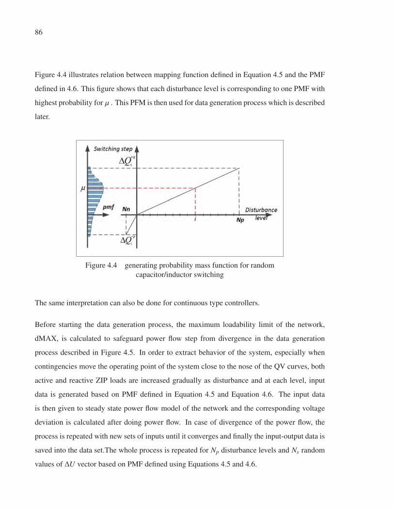
86
Figure 4.4 illustrates relation between mapping function defined in Equation 4.5 and the PMF
defined in 4.6. This figure shows that each disturbance level is corresponding to one PMF with
highest probability for μ . This PFM is then used for data generation process which is described
later.
Figure 4.4 generating probability mass function for random
capacitor/inductor switching
The same interpretation can also be done for continuous type controllers.
Before starting the data generation process, the maximum loadability limit of the network,
dMAX, is calculated to safeguard power flow step from divergence in the data generation
process described in Figure 4.5. In order to extract behavior of the system, especially when
contingencies move the operating point of the system close to the nose of the QV curves, both
active and reactive ZIP loads are increased gradually as disturbance and at each level, input
data is generated based on PMF defined in Equation 4.5 and Equation 4.6. The input data
is then given to steady state power flow model of the network and the corresponding voltage
deviation is calculated after doing power flow. In case of divergence of the power flow, the
process is repeated with new sets of inputs until it converges and finally the input-output data is
saved into the data set.The whole process is repeated for Np disturbance levels and Ns random
values of ΔU vector based on PMF defined using Equations 4.5 and 4.6.

87
Figure 4.5 Algorithm for generating Input-Output data
After generating input-output data set, a two layers feed-forward NN with 100 neurons as
hidden layer is chosen to fit data set. The network is also trained using Levenberg-Marquardt
method for 70% of the generated In-Out data samples as training data and then validated and
tested by the remaining 30%. Figure 4.6 shows error histogram for the identified NN model
after 8 iterations. As can be seen from Figure 4.6, the error between outputs of the identified
model and the output data for the same input instances are normally distributed around zero
with standard deviation less than 0.001 which is acceptable for this problem.
4.4 Simulation Results for IEEE 118-bus power network
To validate the stability and robustness of the proposed controller, the closed loop system is
tested on a real-time dynamic simulator from OPAL-RT technologies. The dynamic model of

88
Figure 4.6 Error histogram for the identified NN sensitivity model
of IEEE 118-bus test case
the power system is defined using ePHASORsim software for which the input data of power
flow as well as dynamic parameters are provided in PSS/e format. The dynamic models used
in this test-case are synchronous generators of type GENROU, static var compensator of type
CSVGN5, excitation systems of type EXST1, maximum excitation limiters of type MAXEX2
and also turbine governors of type TGOV1. Power system stabilizers of type STAB1 are also
connected to excitation systems on buses 26, 49 and 100. In addition, the network includes
35 static var compensator of type CSVGN5. Finally, constant power loads are considered to
represent the capacitor/inductor banks.
Maximum voltage deviation on generator buses are considered to be 0.05p.u. and the minimum
limit is assumed to be −0.05p.u.. Moreover, the capacitor/inductor banks can inject maximum
of 100MV AR and absorb −20MV AR with the switching step of 10MV AR. On the other hand,
voltage on the buses to which the compensators are connected should be between 0.9p.u. and
1.1p.u.. Finally, synchronous generators as well as static var compensators have a reactive
power capacity between −100MV AR and 400MV AR.

89
The parameters of the proposed CSVC used for validation are shown in Table 4.1.
Table 4.1 parameters of the proposed CSVC controller
Parameter ValueNumber of iterations of SA algorithm, T0, for each time step 1000
Diagonal weights of R for generators 0.1
Diagonal weights of R for capacitor/inductor banks 5E-4
Equalization weights for generators, αi j 1E-5
Equalization weights for capacitor/inductor banks, βi j 1E-6
Coefficient, α, in SA flowchart, Figure 4.2 0.0214
The proposed CSVC is tested under different scenarios against linear sensitivity based CSVC
method and also traditional method based on local measurements and control. All three meth-
ods use the same control structure of Figure 4.1, except for the network sensitivity model which
is different. The linear based CSVC uses a linear full matrix sensitivity model while the tradi-
tional controller employs a diagonal sensitivity which just maps local reactive power injection
to local voltage. Also the linear sensitivity based CSVC method uses the same generators and
capacitor/inductor banks as the proposed algorithm while the traditional control method only
uses capacitor/inductors which are installed on the pilot buses. The time step of secondary
voltage controller used in all three cases is 5 seconds.
In the following, the validation scenarios are discussed.
4.4.1 Senario 1: change of reference voltage on the pilot nodes:
In the first scenario, the tracking feature of the proposed CSVC is validated. In this way, the
reference voltage of all pilot nodes are suddenly increased by 3% of per unit at t = 5 seconds.
Figure 4.7 shows the dynamics of the voltage deviation on pilot nodes as well as its steady state
values. As can be seen from Figure 4.7a, after immediate reference change at t = 5 seconds,

90
voltage on pilot nodes does not change instantaneously due to a delay of 5 seconds exists in the
control loop. Consequently, voltage error error shows a gap of 0.03p.u. in the timespan 5−10
seconds. However, at t = 10 seconds, all control approaches except the traditional method take
action, which leads the voltage error to reduce gradually. However for the traditional control
approach, as seen in Figures 4.7a & 4.7b, the voltage error on pilot buses remain unchanged
since none of the capacitor’s installed on the pilots take actions as shown in Figures 4.8b &
4.8c. This is caused by the large switching step of capacitor/inductor banks and also the lack
of continuous type compensators to reduce the error by adjusting the control command with
smaller changes.
Comparing the results shown in Figure 4.7b for the proposed method and linear based CSVC
method, one can see that the steady state voltage error for both controllers are quite the same
with a slightly better performance of the proposed method. However, from Figure 4.7a it can be
seen that the settling time of the proposed method is significantly smaller due to the fact that the
nonlinear NN based model in the proposed CSVC calculates the required reactive power more
precisely at each time step hence the introduced steady state error after applying the control
command is smaller. Moreover oscillatory behavior seen specifically on the voltage error of
bus 43 for the linear based CSVC method does not exist in the proposed method.
Figure 4.8 illustrates the corresponding calculated reference voltage change for AVR connected
to the excitation system of the generators as well as reactive power injection by capacitor/reac-
tor banks. As depicted in Figure 4.8a, the reference voltage of AVRs start to increase with a 5
seconds of delay right after fault for both proposed CSVC and linear sensitivity based CSVC.
However, in the latter, the reference voltage for the AVRs connected to the synchronous ma-
chine at bus 54 saturates at its maximum, i.e. 5%p.u..
Finally, Figure 4.9a illustrates voltage on the buses to which participant generators, static var
compensator and capacitor banks are connected and Figure 4.9b shows the injected reactive
power by participant generators and static var compensators. As can be seen for both proposed

91
CSVC and linear sensitivity based CSVC, terminal voltages and reactive powers are within the
desired limits.
4.4.2 Senario 2: sudden load change:
In this scenario, all the constant impedance loads are suddenly increased by100% at t = 10
seconds, while constant power and constant current loads are increased by 40% and 20% re-
spectively. Reference voltages on pilot buses are considered constant and they are equal to
before contingency values. Figure 4.10 shows the dynamics of the voltage deviation on pilot
nodes as well as its steady state values. As can be seen in this figure, few milliseconds after
disturbance, voltage on pilot buses suddenly drops by 0.3p.u.. However, the primary level
controllers take action immediately and are able to reduce the error to less than 0.1p.u. just in
5 seconds. The steady state error, however, is compensated by the secondary level controllers
starting the first time step, at t = 5 seconds. The dynamic simulations also show a similar
response of the proposed CSVC and the other two methods. Figure 4.10b also illustrates the
steady state error of voltage of the pilot nodes. As can be seen in this scenario, the proposed
CSVC has a similar error to the other two methods.
Figure 4.11 also shows the calculated control signals for both generators and capacitor/inductor
banks. Figure 4.11a illustrates that the reference voltage change for AVR of the machine at
buses 12 and 54 saturate at 25 seconds for the linear based CSVC. However, for the proposed
method only the AVR reference of the machine at bus 12 saturates.
Finally, Figure 4.12a illustrates voltage on the buses to which participant generators, static var
compensator and capacitor banks are connected and Figure 4.12b shows the injected reactive
power by participant generators and static var compensators. As can be seen in Figure 4.12a,
at the time of fault voltage on some control buses drop as low as 0.7p.u.. However due to the
fast reaction of the primary level controllers, they recover back to 0.87p.u. in just 5 seconds
after fault. At t = 10 seconds, both proposed CSVC and linear sensitivity based CSVC take
action and bring back the voltage at control buses within the limit while they try to maintain

92
the voltage on pilot buses. Figure 4.12b also shows that reactive power of generators are kept
within the desired limits except for the time of fault, t = 10 seconds and for the time period
[16.5,19.75] seconds. In both cases, reactive power injected by the synchronous generator
located at bus 100, goes beyond 400MV AR limits. The latter is caused by the fast reaction of
the AVR connected to this machine. However few milliseconds after fault, the reactive power
lowers down to less than the maximum limit. The later violation, on the other hand, occurs
between two time steps of the CSVC and it is not detected by the algorithm. On the other hand,
the CSVC is able to detect reactive power violation of the generator located at bus 49 at t = 15
seconds. Consequently, the CSVC reduces reference voltage of the connected AVR to lower
the reactive power to less than the maximum limit.
4.4.3 Senario 3: bus trip:
In this scenario, buses 15, 80, 94 & 49 are tripped from the network at t = 10 seconds. Trip-
ping these buses disconnects all lines, transformers, generators connected to them and leads
to a topology change in the network. Moreover, one of the tripped buses, i.e. bus 49, has a
participant generator in CSVC attached to it which is also tripped as a result of the bus trip.
Figure 4.13 shows the dynamics of the voltage deviation on pilot nodes as well as its steady
state values. Moreover Figure 4.14 illustrates the dynamics of the control variables for both
generators and capacitor/inductor banks versus time and also steady state values of capaci-
tors/inductors switching steps.
As can be seen in Figure 4.10a, despite major topology change, the proposed controller is able
to compensate voltage error even faster than the other two methods.
The simulations are run on Opal-RT’s OP-4510 Real-time simulator with Intel Xeon E3 4-core
3.5 GHz CPU. Figure 4.15 illustrates the optimization results of the SA algorithm for scenario
3 in which the algorithm is run for 1000 iterations at each time step of the controller. Thus
each 1000 iterations belong to one time step of the controller. As can be seen in this figure, the
objective function value is able to converge at each time step of the controller to a suboptimal

93
solution in less than 100 iterations. However, it is run for 1000 iterations to achieve close to
optimal results. In this simulation, the calculation to find the suboptimal solution is done in
500 milliseconds which is much smaller than the time step of the proposed CSVC loop, i.e. 5
seconds. In this way, the computational delay is negligible and the proposed controller can be
applied in real time for such a network.
4.5 Conclusion and Future Works
In this paper, a new CSVC strategy is proposed which coordinates discrete and continuous type
compensators in transmission system to improve voltage profile at pilot buses of the network
when facing large disturbances. The controller consists of two parts: The identified nonlinear
sensitivity model of the network and an optimizer. The nonlinear sensitivity model is identified
using Neural Networks based on Input-Output data generated from random disturbances on the
network. The optimizer utilizes SA algorithm and is combined with NN model to find the opti-
mal switching of the capacitor/inductor banks after sensing any disturbance. The effectiveness
of the proposed algorithm is tested by applying the controller on IEEE 118-bus power system
while perturbing the network by different levels of disturbance. The simulation results show
that the proposed controller is able to bring voltage back into the desired limits for different
disturbance cases. Beside voltage control the algorithm also minimizes the reactive power in-
jected to the network. Comparing the simulation results of the proposed method with linear
CSVC method and also the traditional approach showed that taking into account the nonlinear
model of the system leads to a faster convergence of the method. However both linear based
CSVC and the proposed methods had the same steady state voltage error. Moreover it was
observed that the traditional method is not able to track the reference voltage change while the
other two can compensate the tracking error.
Future works toward improvement of the proposed controller can be considered as follows.
As has been discussed in Section 4.4 the NN model is identified off-line, and remains un-
changed during the implementation phase. One suggestion is to use adaptive learning methods
in real-time to adapt the NN model with changes in the power network. On the other hand, the

94
proposed strategy was implemented as a centralized controller. This method can be modified
to be applied in a decentralized way on the multi-area power networks. In this way, the inter-
action of areas with each other as well as coordination of the regional CSVC controllers may
be considered in control design.
Finally, it was assumed in this paper that the pilot nodes are fixed. However, in case of major
events or contingencies, these identified nodes might change. In this way, a comprehensive
sensitivity analysis could be done to identify all the potential pilot nodes for different types
of contingencies and network base cases. Afterwards, a nonlinear model can be identified
assuming voltage of all these potential pilot nodes as outputs. In this way, for each operating
condition, a subset of these nodes are controlled while assuming zero weighting coefficients for
the voltage error term of other nodes which are not considered as pilot buses for this specific
scenario.
4.6 Acknowledgment
The authors would like to thank Opal-RT Technologies for providing dynamic data for IEEE118
bus power system and also for the real-time simulator and ePHASORsim software license.

95
a) Voltage error on the pilot buses
b) Steady state voltage error on the pilot buses
Figure 4.7 Scenario 1: Proposed method (solid line), Linear sensitivity based CSVC
(dotted line) and Traditional method (dashed line)

96
a) Change of reference voltage of AVRs connected to generators
b) Reactive power injection by capacitor/inductor banks
c) Steady state reactive power injection by capacitor/inductor banks
Figure 4.8 Scenario 1: Proposed method (solid line), Linear sensitivity based CSVC
(dotted line) & Traditional method (dashed line)

97
a) Voltage on participant generator and capacitor buses
b) Injected reactive power by generators
Figure 4.9 Scenario 1: Proposed method (solid line), Linear sensitivity based CSVC
(dotted line) & Traditional method (dashed line)
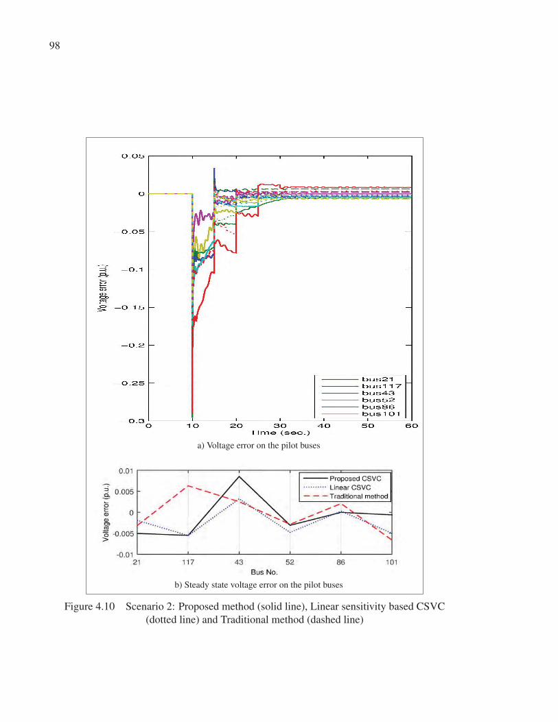
98
a) Voltage error on the pilot buses
b) Steady state voltage error on the pilot buses
Figure 4.10 Scenario 2: Proposed method (solid line), Linear sensitivity based CSVC
(dotted line) and Traditional method (dashed line)

99
a) Change of reference voltage of AVRs connected to generators
b) Reactive power injection by capacitor/inductor banks
c) Steady state reactive power injection by capacitor/inductor banks
Figure 4.11 Scenario 2: Proposed method (solid line), Linear sensitivity based CSVC
(dotted line) & Traditional method (dashed line)

100
a) Voltage on participant generator and capacitor buses
b) Injected reactive power by generators
Figure 4.12 Scenario 2: (Proposed method (solid line), Linear sensitivity based CSVC
(dotted line) & Traditional method (dashed line)

101
a) Voltage error on the pilot buses
b) Steady state voltage error on the pilot buses
Figure 4.13 Scenario 3: Proposed method (solid line), Linear sensitivity based CSVC
(dotted line) and Traditional method (dashed line)

102
a) Change of reference voltage of AVRs connected to generators
b) Reactive power injection by capacitor/inductor banks
c) Steady state reactive power injection by capacitor/inductor banks
Figure 4.14 Scenario 3: Proposed method (solid line), Linear sensitivity based CSVC
(dotted line) & Traditional method (dashed line)

103
Figure 4.15 Evolution of the objective function at each time step of the controller


CHAPTER 5
SECONDARY VOLTAGE CONTROL WITH CONSENSUS BETWEEN REGIONALCONTROLLERS
Arvin Morattab1, Ouassima Akhrif1, Maarouf Saad1
1 Department of Electrical Engineering, École de Technologie Supérieure,
1100 Notre-Dame Ouest, Montréal, Québec, Canada, H3C 1K3
Article submitted for publication, February 2018
Abstract
SVC is a well-known control strategy to improve mid-term voltage stability in a region. It
is based on partitioning the power system into electrically decoupled areas and controlling
the voltage of pilot buses as representative nodes of each area in a decentralized way. In
practice however, these control areas are not completely decoupled and some compensators in
one area might affect a pilot bus of a neighbor area. In this case, a coordination is required
between the regional SVCs to reach a consensus for the action of such compensators. This
paper proposes a novel consensus based SVC strategy for coordination between neighbor areas
of a power grid. In this way, for each group of regional SVCs with shared compensators, a
higher level coordinator is defined which calculates the consensus values for all conflicting
pairs based on a proposed consensus protocol. The consensus is reached in two iterations
between SVCs and the coordinator. It is shown through simulations that the proposed strategy
can diminish oscillations caused by uncoordinated regional SVCs while minimizing reactive
power efforts. IEEE 118 bus test-case is used to validate the effectiveness and performance of
the proposed algorithm on a real-time simulation test-bench in which the regional SVCs are
run on separate computational cores. The communication between SVCs, measurement units
and compensators are through standard IEEE C37.118 and DNP3 protocols.

106
Introduction
SVC is widely used nowadays in power system control centers as part of hierarchical control
strategy to ameliorate voltage stability all over the power grid. Various implementations of
SVC Corsi (2015) have been successfully employed in many countries such as France, Italy,
Brazil, Romania, China and USA. Although voltage control is essentially a local problem, it
has been proven that SVC, which emphasizes on voltage control in an area of the power system,
can improve voltage stability by managing reactive power resources considering their limits to
contribute to the voltage control of representative buses of each area, called pilot buses.
The first step toward SVC is to allocate pilot buses and to partition the power system into elec-
trically decoupled coherent regions. There are many methods presented in the literature which
discuss this issue Lagonotte et al. (1989); Conejo et al. (1994); Karakatsanis & Hatziargyriou
(1994); Conejo & Aguilar (1998); Amraee et al. (2010); Trakas et al. (2014); Mezquita et al.
(2015); Mehrjerdi et al. (2013b,c); Cotilla-Sanchez et al. (2013); Amadou et al. (2014); Chen
et al. (2015); Alimisis & Taylor (2015). These methods are mostly centered around the idea
of sensitivity analysis presented in Corsi (2015). The control buses are also identified for each
control area using the same approach used for pilot nodes. Finally, the SVC control loop is
established in each area as a two-level PI rule which measures the voltage on the pilot bus and
sets the set-point of the PVC such as the AVR or static var compensators. This method lacks
the coordination of SVC of two neighbor regions in the case when some compensators affect
voltage of the two neighbor areas substantially.
To resolve this issue, Paul et al. (1987) presents Coordinated SVC in which the two intercon-
nected areas form one region and a MIMO optimal controller is proposed to regulate voltage
on the pilot buses.
Although this approach overcomes the problem of uncoordinated SVCs by unifying the two, it
is not in favor of the deregulated structure of nowadays power grids in which the focus is on
decentralization of the power system. In this way, a lot of research has been done to find decen-
tralized control algorithms that consider coordination between neighbor areas. In this regard,

107
Mehrjerdi et al. (2013d) proposes a coordination strategy in which the interaction between
areas is defined using a connection matrix. The effect of areas on each other is considered
as the measured tie-line reactive power between the two neighbors. Moreover, Moradzadeh
et al. (2013) uses distributed MPC algorithm for SVC in which each SVC considers the con-
trol action taken by its neighbors in the last time step to calculate its current control law. Also
Morattab et al. (2017a) presents a decentralized MPC approach in which the effect of the neigh-
bor areas is measured as tie-line reactive power and defined as a measured disturbance. While
in these methods each regional SVC assumes the effect of its neighbors, there is no iteration
between neighbor areas at one time step. The coordination of one area and its neighbor is
basically based on the measured signals from the neighbors in the last time step.
In recent years, a growing amount of research has focused on multi-agent based cooperative
SVC in transmission network in which the regional controllers reach a consensus at each time
step Vaccaro et al. (2011); Loia et al. (2013); Bottura & Borghetti (2014); Su et al. (2016);
Borghetti et al. (2017).
In this way, Vaccaro et al. (2011) proposes a decentralized non-hierarchical voltage regula-
tion architecture in which the states of the neighbor areas dynamics are synchronized to the
weighted average of the variables sensed by all the controllers in the smart grid. Moreover,
Loia et al. (2013) proposes decentralized and non-hierarchal voltage control architecture based
on cooperative fuzzy agents to achieve consensus. In addition, Bottura & Borghetti (2014)
and Borghetti et al. (2017) discuss an asynchronous leaderless multi agent approach that co-
ordinates the reactive power compensators. Finally, Su et al. (2016) formulates CSVC as a
nonlinear successive ∞-norm minimization problem in which the load disturbances are esti-
mated on-line.
The methods presented in Vaccaro et al. (2011) & Loia et al. (2013), define consensus as
convergence to the average of the measurements and needs a quite large number of iterations,
resulting therefore into a large number of exchange data. However, due to the local nature
of voltage control problem, it is not required to reach a global consensus. In this way the

108
consensus could be just limited to the neighbor areas which are strongly coupled. On the
other hand, the so-called gossip based approach presented in Bottura & Borghetti (2014) and
Borghetti et al. (2017) requires some time to evaluate the priorities and come up with an action.
By limiting the consensus strategy just to the strongly coupled neighbors, the required time for
the gossip based method can be saved tremendously.
This paper presents a novel coordination technique in a multi area power systems between
SVCs belonging to neighbor areas with common buses. Such a consensus is required espe-
cially when the overlapping buses include some compensators which can potentially affect the
voltage of the pilot bus on all neighboring areas. These compensators are called shared com-
pensators throughout this paper. In the proposed method, each regional SVC calculates the
control set- point for the PVC of these shared compensators as well as its non-shared com-
pensators. The calculated values for the former group by all SVCs of the overlapping areas
might conflict with each other. These conflicting values alongside their corresponding solution
of their local objective function are then communicated to a coordinator which resolves the
conflicts by establishing a consensus protocol between all the participant SVCs. Such a deci-
sion is made by first a linear estimation of the pareto front of the optimization problems solved
first locally and then calculating the consensus value for the PVC of the shared compensator
by minimizing the weighted sum of all linearized objective value deviations of the overlapping
areas. In the second iteration, the error caused by the consensus is corrected by communicating
back the calculated consensus values to the regional SVCs and re-evaluating the set-points of
the regional PVCs. as known.
The novelties of this paper are enumerated as follows:
• Propose a novel consensus strategy for multi-objective optimization problems;
• Propose a modified version of sensitivity analysis presented in Corsi (2015) in which control
regions can overlap. Some compensators might be selected for SVC which belong to the
shared area;

109
• Validate on a real-time simulator the iterative consensus algorithm with optimization based
SVCs to show its feasibility to be implemented on real power systems.
The paper is organized as follows: Section 5.1 describes the proposed methodology in which
the modified sensitivity analysis is presented which is then followed by the proposed consensus
strategy. In Section 5.2, the case-study which is the IEEE 118 bus power system is presented.
The results of applying modified sensitivity analysis to find pilot nodes, partitioning the net-
work and allocation of the control buses is also discussed in this section. Section 5.3 presents
the real-time test-bench on which the simulation scenarios, discussed in Section 5.4, are run
and validated. Finally, Section 5.5 concludes the paper and discusses future works.
5.1 Methodology
5.1.1 Modified sensitivity analysis to partition the network
The classical sensitivity analysis method presented in Corsi (2015), relies on successive re-
ordering of the sensitivity matrix relating reactive power injection to voltage deviation on all
load buses of the grid. The first pilot node is considered as the bus with the strongest short
circuit capacity and afterwards, all buses with their coupling coefficient to this node larger
than a predefined threshold, are assumed to belong to the first control region. These buses are
therefore excluded from subsequent pilot node searching procedure. This process repeats for
the remaining buses until the short circuit capacity of the selected candidate is smaller than
minimum requirement for a pilot bus. It should be noted that there might be some buses which
are identified to belong to more than just one region. However, for such a bus, the coupling
factor to the pilot nodes of all areas between which the bus is shared is compared and the bus
is assumed to be owned or better to belong to the area with the highest coupling factor. Finally,
the last step is to find the most effective compensators in each area, i.e. controllers which have
the highest sensitivity to the regional pilot node.
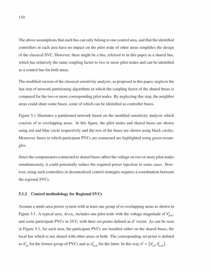
110
The above assumptions that each bus can only belong to one control area, and that the identified
controllers in each area have no impact on the pilot node of other areas simplifies the design
of the classical SVC. However, there might be a bus, referred to in this paper as a shared bus,
which has relatively the same coupling factor to two or more pilot nodes and can be identified
as a control bus for both areas.
The modified version of the classical sensitivity analysis, as proposed in this paper, neglects the
last step of network partitioning algorithms in which the coupling factor of the shared buses is
compared for the two or more corresponding pilot nodes. By neglecting this step, the neighbor
areas could share some buses, some of which can be identified as controller buses.
Figure 5.1 illustrates a partitioned network based on the modified sensitivity analysis which
consists of m overlapping areas. In this figure, the pilot nodes and shared buses are shown
using red and blue circle respectively and the rest of the buses are shown using black circles.
Moreover, buses to which participant PVCs are connected are highlighted using green rectan-
gles.
Since the compensators connected to shared buses affect the voltage on two or more pilot nodes
simultaneously, it could potentially reduce the required power injection in some cases. How-
ever, using such controllers in decentralized control strategies requires a coordination between
the regional SVCs.
5.1.2 Control methodology for Regional SVCs
Assume a multi-area power system with at least one group of m overlapping areas as shown in
Figure 5.1. A typical area, Areai, includes one pilot node with the voltage magnitude of ViPN ,
and some participant PVCs in SVCi with their set-points defined as ui vector. As can be seen
in Figure 5.1, for each area, the participant PVCs are installed either on the shared buses, the
local bus which is not shared with other areas or both. The corresponding set-point is defined
as uish for the former group of PVCs and as ui
nsh for the latter. In this way ui ={ui
sh, uinsh
}.

111
Figure 5.1 A group of overlapping areas partitioned using modified sensitivity analysis;
pilot nodes (red nodes), shared buses (blue circles), nodes with participant compensator
(highlighted using green rectangles)
A typical optimization problem solved by SVCi is shown in Equations 5.1.

112
ΔViPN = fi(ui
nsh − uinsh(k −1), ui
sh − uish(k −1))
J∗i = minuinsh,ui
sh
Ji = minuinsh,ui
sh
��V diPN −Vi
PN −ΔViPN
��+(ui
nsh
)Tαi
nshuinsh +
(ui
sh
)Tαi
shuish
s.t :
uimin < ui < ui
max
(5.1)
In this formulation, fi is a function which relates variation of shared and non-shared PVCs’
set-points from their previous values, uish(k − 1) and ui
nsh(k − 1) respectively, to the estimated
voltage deviation on pilot node for Areai, defined as ΔViPN . Moreover, V di
PN is the reference
voltage of the pilot node of Areai which is dictated by the tertiary level controller. Also, αish
and αinsh are the weighting matrices for unknown control set-points, for the PVCs of both shared
and non-shared compensators. Finally, uimin and ui
max are minimum and maximum limits for
the set-points of the PVCs in Areai. Moreover, the computed optimal value for the set-points
of shared and not-shared variables are defined as ui∗sh and ui∗
nsh respectively.
The optimization problem formulated in Equations 5.1 is solved using the method presented in
4. An adapted version of this method is shown in Figure 5.2.
In this figure, the mathematical relation between control set-points and voltage of the pilot
node, defined as functions fi in Equations 5.1, is considered as a nonlinear NN. The optimiza-
tion problem is then solved using SA through an iterative process between the model and the
optimizer.

113
At each iteration, SA algorithm slightly disturbs the current value of set-point solution vector,
ui. The solution is accepted if it first meets all the constraints and second reduces the objective
function of the optimization problem. Otherwise, the SA algorithm uses the value from the last
iteration. This process is repeated so that finally an exit criterion is met. This criterion could
be defined either as a certain threshold for the objective function or the time limit in which the
procedure must be completed. In this way, the last solution is considered as the sub-optimal
control set-points and then sent to all PVCs in Areai.
Figure 5.2 Secondary voltage control using neural network and SA

114
5.1.3 Architecture of the proposed consensus based SVC algorithm
Figure 5.3 illustrates the architecture of the proposed method. As can be seen in this figure,
each regional SVC receives the measured voltage magnitude, ViPN , from the area’s pilot node
and sends back the calculated control set-points for PVCs, ui∗, to the grid. On the other hand,
all the regional SVCs of the overlapping areas communicate with a higher level coordinator
which is responsible of reaching a consensus for the set-point value of the PVC for shared
compensators.
A flow-chart describing the interaction between the power grid, SVCs and also the consensus
coordinator to calculate regional PVC set-points at one time step of the controller is shown in
Figure 5.4. The procedure here is described for one typical SVC, i.e. SVCi, and it would be
the same for the rest.
As shown in Figure 5.4, the procedure consists of two iterations for solving the regional SVC
problem with a consensus step in the middle. In the first iteration, the regional SVCi receives
the measured voltage magnitude, ViPN , from the measurement unit installed on the network.
Next the regional SVC calculates the set-points, uish and ui
nsh, for shared and non-shared PVCs
respectively. This is done by solving the optimization problem described in Section 5.1.2.
It should be noted that the calculated value for a specific shared compensator by one SVC,
might be different from the one calculated by the other SVC. However, at the end, only one
value should be sent to the corresponding PVC in the network. In this regard, in the next
step, the calculated optimal set-points for the PVC of all the shared compensators, i.e. ui∗sh
for i = 1, · · · ,m, is sent to consensus coordinator unit which resolves the conflicts between the
SVCs. For the proposed algorithm, additional information is required by the coordinator unit to
calculate the consensus values. Namely, the optimal value of the objective function at the first
iteration of SVCi solution, J∗i , as well as the linear sensitivity matrix of the objective function
to the set-point of PVCs for shared compensators, defined as Si. The methodology used by
consensus coordinator is described in Section 5.1.4.
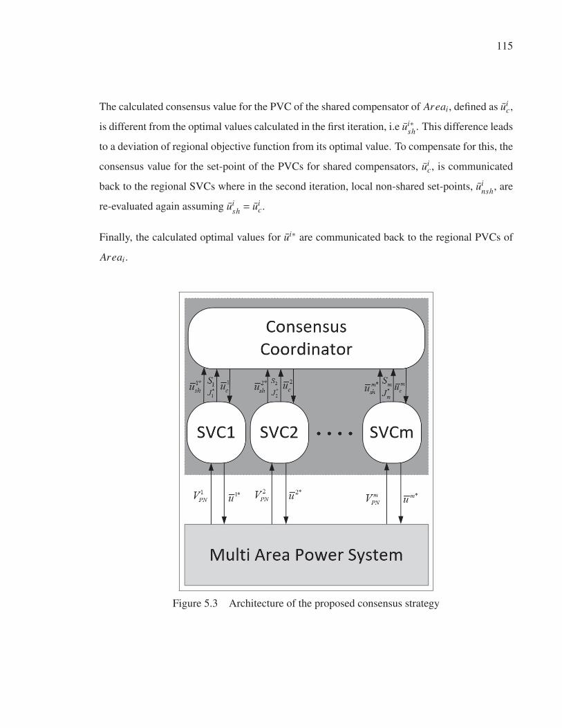
115
The calculated consensus value for the PVC of the shared compensator of Areai, defined as uic,
is different from the optimal values calculated in the first iteration, i.e ui∗sh. This difference leads
to a deviation of regional objective function from its optimal value. To compensate for this, the
consensus value for the set-point of the PVCs for shared compensators, uic, is communicated
back to the regional SVCs where in the second iteration, local non-shared set-points, uinsh, are
re-evaluated again assuming uish = ui
c.
Finally, the calculated optimal values for ui∗ are communicated back to the regional PVCs of
Areai.
Figure 5.3 Architecture of the proposed consensus strategy

116
5.1.4 Consensus coordinator
The consensus coordinator, shown in Figure 5.3, solves the following optimization problem:
minuc
∑mi=1ωi
��Ji − J∗i��2
s.t :
uminc < uc < umax
c
(5.2)
In this formulation Ji − J∗i is defined as the linearization of Equations 5.1 around the optimal
solution, ui∗sh, found in the first iteration of the algorithm described in Figure 5.4. The linearized
equations are as follows:
Ji − J∗i = Si(uic − ui∗
sh) i = 1, · · · ,m (5.3)
In Equation 5.3, Si is the sensitivity of Ji to uish. This sensitivity matrix can be calculated by
disturbing uish around the local minima points and measuring the objective functions’ devia-
tions. Moreover, uic is a vector of consensus values for the set-point of shared compensators
in Areai and uc =[u1
c, · · · , umc]
is the vector of consensus values for all the shared compen-
sators. Finally, ωi is the weighting coefficient to prioritize the importance of each area for the
consensus coordinator.
The corresponding consensus values for each area are then sent back to the regional SVCs to
solve the second iteration of the SVCi based on Figure 5.4.

117
5.1.5 Interpretation of consensus coordinator for two overlapping areas
The optimization problem formulated in Equation 5.1 is solved simultaneously by all SVCi
for i = 1, · · · ,m in the first iteration of the proposed algorithm described in Figure 5.4. Instead
of solving each problem individually for Areai, if one tries to solve all these optimization
problems together, it could be in fact considered as a multi-objective optimization problem
in which ush =[u1
sh, · · · , umsh
]is considered as the set of all shared variables between all the
regional optimization problems. This multi-objective optimization problem does not have a
unique solution and instead there exists a set of pareto-optimal solutions.
As an example, for two overlapping areas with one shared compensator, a pareto-front curve
is depicted in Figure 5.5 using a dashed arc which is defined as the locus of all pareto optimal
solutions. As can be seen in this figure, starting from an initial solution, I, in the feasible region,
shown as the shaded area, the solution of the local optimization problem by each regional SVC
in the first iteration leads to different local minimas, E1 and E2, which are also on the pareto-
front curve. The solutions for the shared variable, u1sh and u2
sh, by each regional SVC is defined
by u1∗sh and u2∗
sh respectively. The corresponding optimal values for the objective functions are
also defined as J∗1 and J∗2 respectively.
For two overlapping areas with one shared variable, u1c , the linearized equations would be as
follows:
J1 − J∗1 = S1(u1c −u1∗
sh)
J2 − J∗2 = S2(u1c −u2∗
sh)
(5.4)
In this way, any arbitrary value for u1c ranging from u1∗
sh to u2∗sh corresponds to an equivalent
point, C, on the line segment between E1 and E2 in Figure 5.5. This line segment can be
interpreted as the linear approximation of the pareto-front curve.

118
Analogously,��J1 − J∗1
��2and
��J2 − J∗2��2
correspond to the square of the length of sides, BC and
AB respectively in the ABC right triangle shown in Figure 5.5. Also, based on the Pythagorean
theorem, the consensus objective function in Equation 5.2, with the assumption of ω1 =ω2 = 1,
is basically the square of the hypotenuse of ABC triangle, i.e. AC. In other words, solving the
consensus optimization problem for the two overlapping areas with one shared compensator is
equivalent to finding a point on E1E2 line which minimizes the distance between point A and
the line segment E1E2. This optimal point, defined as C∗, is basically the intersection point
between the line segment E1E2 and a perpendicular line from A.
5.2 Simulation case study: IEEE 118 bus network
IEEE118 bus power system, used as the test-case, is shown in Figure 5.6. This network has
19 generator units, including synchronous generators of type GENROU, excitation systems
of type EXST1, maximum excitation limiters of type MAXEX2 and also turbine governors of
type TGOV1. Power system stabilizers of type STAB1 are also connected to excitation systems
on buses 26, 49 and 100. In addition, the network includes 35 static var compensators of type
CSVGN5. The loads are considered to be ZIP loads with 40% as constant power, 30% as
constant impedance and 30% as constant current load. Reactive power limit for all static var
compensators as well as generators participating in SVC algorithm is considered to be the same
and defined as: Qmin = −300MVar & Qmax = +300MVar . Moreover the reactive power limits
for participant capacitor/inductor banks are the same and they are defined as: Qmin =−50MVar
& Qmax = +10MVar . Base Power for the test case is 100MV A and the nominal frequency is
50Hz.
The modified sensitivity analysis is used to find pilot nodes and also partition the network.
Using the same parameter names for sensitivity analysis as Corsi (2015), the parameters γ and
εp are found by trial and error to have a good voltage profile on remote buses. In this way
γ = 1E − 3 and εp = 1E − 6. This choice of parameters leads to allocation of 6 pilot nodes
shown as shaded-fill rectangles in Figure 5.6 and are listed as buses 117, 21, 44, 52, 101 and
86. Each of these pilot nodes represents one corresponding control area with borders shown

119
using dashed lines in Figure 5.6. As can be seen, unlike the classical sensitivity method, the
control areas have overlap in some buses. For example, Area 1 has one shared bus, bus 33, with
Area 2 and also two shared buses with Area 3, buses 8 and 17. However the only shared bus
which is identified as a control bus is bus 49 which is shown as shaded region between Area 2
and Area 4. In this way, the proposed consensus strategy is applied to coordinated Area 2 and
Area 4.
The continuous type compensators are allocated at buses 12, 34, 49, 54, 85, 87 and 100 (static
var compensators on buses 34 and 85 and synchronous generator on the rest). Moreover dis-
crete type compensators which are basically capacitor/inductor banks are allocated at buses
117, 20, 21, 22, 23, 43, 44, 45, 51, 52, 53 and 58. All the control buses are shown using ovals
in Figure 5.6.
5.3 Real-time test bench
The validation of the proposed control strategy is done on a real-time simulation target, OP4510,
from OPAL-RT Technologies. Beside real-time capabilities to validate the performance of
complex control strategies, OP4510 offers the possibility to implement simulations on multi-
cores in parallel and also to support different industrial communication protocols used in real
power systems. This makes it easy to validate distributed control architectures such as the
proposed method. The software used to simulate the dynamics of the power system is ePHA-
SORsim from OPAL-RT which is a phasor-domain solver Jalili-Marandi et al. (2013),Opal-RT
(2018). It benefits from state of the art techniques to improve performance and accuracy of
simulations for large-scale power grids. It also includes a rich built-in and Modelica based
library of different power system components and also supports importing data from various
power system stability analysis tools such as PSS/e and CYME.
Figure 5.7 illustrates the configuration of the test-bench to validate the proposed consensus
strategy in real-time. The software interface to develop the test-bench is Simulink from Math-
Works in which OPAL-RT’s ePHASORsim block is used to define the power network. The data

120
is also sent through a communication channel with a Gaussian noise model in which the SNR
is 100 dB. The communication protocol to send measured data from power gird (i.e. voltage on
pilot buses) to the regional SVCs is IEEE C37.118 which is used by PMUs in real power grids.
OPAL-RT’s library supports both slave (sending) and master (receiving) C37.118 protocols.
Moreover, the control commands from the DCSVCs are sent to the network using Ethernet
protocol. As can be seen from Figure 5.7, a dedicated communication channel is defined to
send and receive data from each area of the power grid. Such an architecture is also in-line
with the requirements of multi-TSO power grids. To cope with the decentralized architecture
of the proposed control strategy, regional SVCs as well as power network model are located in
separate subsystems labeled as Corei,M ASTE R/SL AVE . The convention of master and slave
subsystems are used by RT-LAB to inform the compiler during code generation process that
each subsystem’s generated code is transferred and run in a separate physical core on the target
computer. In this way, computations on each core are done in parallel with the other cores and
the performance of each subsystem can be measured separately without having any overloads
caused by other subsystems. Although in this paper the method presented in 4 is adapted for
SVC, the proposed test-bench can be used to run and validate any other decentralized control
strategy.
5.4 Simulation Results
To validate the proposed control strategy, two different simulation scenarios are considered
to be applied on IEEE 118 bus power system. The simulation results for the cases with and
without consensus strategy are compared accordingly. It should be noted that for the case with-
out consensus, the average calculated set-point by the neighbor SVCs is calculated. However,
unlike the consensus strategy, this calculated value is directly applied to the corresponding
PVC without having any iteration between SVCs and shared PVCs. In the following, each
simulation scenario is discussed in detail.

121
5.4.1 Scenario 1- Sudden Load variation
In this scenario, all the constant impedance loads are suddenly increased by100% at t = 10
seconds, while constant power and constant current loads are increased by 40% and 20% re-
spectively. Reference voltages on pilot buses are considered constant and they are equal to
before contingency values. Figure 5.8 shows the dynamics of the voltage deviation on pilot
nodes. As can be seen in this figure, few milliseconds after disturbance, voltage on pilot buses
suddenly drops by 0.08p.u.. However, the PVCs take action immediately and are able to re-
duce the error to less than 0.03p.u. in less than 10 seconds. The steady state error, however, is
compensated by the SVC control loop starting the first time step, at t = 20 seconds. Comparing
the voltage on pilot buses 44 and 52 for the cases with and without consensus strategy, one
can see that steady state error for bus 44 gradually decreases with consensus between SVCs
of Area 2 and Area 4 as well as PVC of the local controller. However for the case with no
consensus the error remains constant. Moreover for the bus 52, the case without consensus has
led to big overshoot at t = 20 seconds, while the consensus based controller is able to diminish
such an overshoot.
Figure 5.9a also shows the calculated reference voltage deviation for AVR connected to the
synchronous generators while Figure 5.9b illustrates the reactive power injection by capaci-
tor/inductor banks.
5.4.2 Scenario 2- Reference Voltage change
In this scenario, the reference voltage of all pilot nodes are suddenly increased by 3%p.u. at
t = 5 seconds.
Figure 5.10 shows the dynamics of the voltage deviation on pilot nodes. As can be seen from
this figure, after reference change at t = 5 seconds, voltage on pilot nodes does not change
hence leads to sudden error of 0.03p.u.. However, at t = 10 seconds, both controllers, with and
without consensus take action which leads the voltage error to reduce gradually. However for
the case without consensus strategy, it can be seen that the voltage on pilot bus 52 has a large

122
overshoot which diminishes after some oscillations while such a behavior is not seen form the
controller with consensus strategy. On the other hand, same as scenario 1, the controller with
consensus strategy is able to reduce the steady state error on bus 44 in less than 60 seconds
while it remains constant for the case without consensus.
Figure 5.11a also shows the calculated reference voltage deviation for AVR connected to the
synchronous generators and also Figure 5.11b illustrates the reactive power injection by capac-
itor/inductor banks.
5.4.3 Real-time performance validation
The simulations test-bench presented in 5.3 is used to validate real-time performance of the
proposed controller. In this simulation, the maximum calculation time, between all SVCs, to
find the suboptimal solution is 700 milliseconds which is much smaller than the time step of the
SVC loop, i.e. 10 seconds. In this way, the computational delay is negligible and the proposed
controller can be applied in real time for such a network.
5.5 Conclusion and Future Works
In this paper, a new sensitivity analysis method was used to (i) find the pilot nodes, (ii) parti-
tion the network and finally (iii) allocate the controllers. For the case where a control bus is
identified to be a shared compensator, a consensus strategy is proposed in which the regional
SVCs as well as the corresponding PVC reach an agreement in an iterative process. Simu-
lation results showed that such a consensus strategy reduces the overshoots and oscillations
due to the lack of coordination between regional SVCs. Moreover the consensus strategy was
able to reduce the steady state error on the pilot buses corresponding to the areas with shared
compensators.

123
Figure 5.4 Flowchart describing the interaction of SVC of Area i
and the consensus coordinator

124
Figure 5.5 Pareto-front curve of a two-objective optimization problem
with its linear estimation

125
Figure 5.6 IEEE 118-bus power network. Pilot nodes (solid rectangle) and control bus
(dashed rectangle)

126
Figure 5.7 Configuration of the real-time test-bench for validation of DCSVC algorithm

127
Figure 5.8 Scenario 1: Voltage error on the pilot buses. With consensus strategy
(solid line), without consensus strategy (dotted line)

128
a) Change of reference voltage of AVRs connected to generators
b) Reactive power injection by capacitor/inductor banks
Figure 5.9 Scenario 1: With consensus strategy (solid line), Without consensus strategy
(dotted line)

129
Figure 5.10 Scenario 2: Voltage error on the pilot buses. With consensus strategy
(solid line), without consensus strategy (dotted line)

130
a) Change of reference voltage of AVRs connected to generators
b) Reactive power injection by capacitor/inductor banks
Figure 5.11 Scenario 2: With consensus strategy (solid line), Without consensus
strategy (dotted line)

CONCLUSION AND RECOMMENDATIONS
Conclusion
This thesis proposed novel approaches regarding to analysis and design of multi-agent coordi-
nated SVC in transmission networks.
In the first chapter, an introduction to the fundamental concepts of voltage stability and control
was presented. The chapter also discussed the classical SVC algorithm in which the advantages
as disadvantages of the method were enumerated. CSVC method was then discussed as an
alternative approach to overcome drawbacks of the SVC method.
Then in chapter 2 a timely review of the works related to SVC was done in which the literature
was classified according to different aspects of the SVC problem. The chapter also analyzed
recent literature based on which the methodologies and novelties of the this thesis were ad-
dressed.
Chapter 3 proposed a decentralized MPC scheme for coordinated secondary voltage control of
large-scale multi-area highly interconnected power networks. The controllers were designed in
a decentralized way for each area which modifies reference signal of reactive power compen-
sator devices. The interactions between neighboring areas were considered as measured reac-
tive power deviation on tie-lines between these areas. This value was defined as a measured
disturbance for MPC in each area. The simulation results for the proposed method showed that
the decentralized controllers are able to both regulate and track the desired voltage in presence
of external disturbances. It was also shown that considering the delay model in each regional
MPC model improves the stability of the closed loop system.
The proposed algorithm was also tested on a realistic power grid with 5000 buses in real-time
considering the communication protocols and the model of the communication channel. The

132
real-time performance of the proposed method confirms that the proposed method is computa-
tionally feasible and scalable to large scale power grids.
Despite effectiveness of the proposed method, some difficulties were also observed. The pro-
posed MPC method is based on the identified linear model of the system. In this way, the model
might not be valid for extreme disturbance cases. Moreover, the control signals calculated by
the proposed MPC method are continuous type by nature. Although one can discretize the
continuous values and apply them to discrete type compensators, it might lead to oscillatory
behavior of the closed loop system when the discrete steps are large. Using hybrid (mixed
continuous and discrete) MPC approaches on the other hand requires a large amount of com-
putational effort to solve the optimization problem.
To overcome these issues, in chapter 4, a new CSVC strategy was proposed which coordinates
discrete and continuous type compensators in transmission system to improve voltage profile at
pilot buses of the network when facing large disturbances. The controller consists of two parts:
The identified nonlinear sensitivity model of the network and an optimizer. The nonlinear sen-
sitivity model is identified using Neural Networks based on Input-Output data generated from
random disturbances on the network. The optimizer utilizes SA algorithm and is combined
with NN model to find the optimal switching of the capacitor/inductor banks after sensing any
disturbance.
The comparison of the results of the proposed method with the linear model based CSVC and
also traditional method in which only capacitor banks are utilized, shows that the proposed
method has a faster response to load variation, sudden disturbances as well as change of the
pilot nodes’ reference voltage. The steady state error of the proposed method is also smaller
than the traditional method and similar to the linear based CSVC. Beside voltage control, the
proposed algorithm also minimizes the reactive power injected to the network.

133
Due to the local nature of the voltage control problem, solving a centralized optimization prob-
lem as proposed in chapter 4 might not be computationally beneficial for larger power systems
with more control variables. On the other hand, while solving the optimization problem in a
decentralized way, one should take into account the effect of the control actions on the neighbor
areas to avoid any uncoordinated behavior.
This issue was investigated in chapter 5, in which a modified sensitivity analysis method was
used to (i) find the pilot nodes, (ii) partition the network and finally (iii) allocate the controllers.
For the case where a control bus is identified to be a shared compensator, a consensus strategy
is proposed in which the regional SVCs as well as the corresponding PVC reach an agreement
in an iterative process. Simulation results showed that such a consensus strategy reduces the
overshoots and oscillations due to the lack of coordination between regional SVCs. Moreover
the consensus strategy was able to reduce the steady state error on the pilot buses corresponding
to the areas with shared compensators.
Future Works
Minimize the number of switching for discrete type compensators
Although the proposed method in chapter 3 can be generalized to other types of reactive com-
pensators such as tap-changers, capacitor banks, synchronous condensers and other FACTS
devices, certain considerations should be taken into account for switching based devices such
as capacitor banks or tap-changers. The number of switching of such devices should be mini-
mized as much as possible to avoid long-term damages. Moreover, due to the discrete nature of
these devices, the optimization problem leads to a mixed integer linear or quadratic program-
ming which can be solved using available methods.

134
Using physical modeling
Another possible improvement to the proposed method in chapter 3 is to use physical model-
ing instead of black-box system identification to have more accurate and meaningful models.
Having linearized symbolic models of different components of the power system, one can eas-
ily formulate the MPC optimization problem symbolically which leads to a more flexible and
performant approach which can easily be adapted for any power system.
Considering dynamics of the load
On the other hand, considering different load models and their dynamics can lead to more
accurate formulation of voltage stability problem. Considering the dynamics of the load in the
MPC formulation can provide more accurate control when loads are constantly changing in the
power grid.
Considering the effect of unknown communication delays
The effect of unknown communication delays on the stability of the controller can be consid-
ered as a future work. Such an assumption is more realistic for delays caused by cyber attacks
since it is not in control of the power system utilities and they may not have any statistic data
to estimate the value.
Use adaptive learning methods for neural network
As was discussed in Section 4.4, the NN model is identified off-line, and remains unchanged
during the implementation phase. One suggestion is to use adaptive learning methods in real-
time to adapt the NN model with changes in the power network. On the other hand, the pro-
posed strategy was implemented as a centralized controller.

APPENDIX I
MODEL PREDICTIVE COORDINATED SECONDARY VOLTAGE CONTROL OFPOWER GRIDS
Arvin Morattab1, Asber Dalal2, Ouassima Akhrif1, Maarouf Saad1, Serge Lefebvre2
1 Department of Electrical Engineering, École de Technologie Supérieure,
1100 Notre-Dame Ouest, Montréal, Québec, Canada, H3C 1K32 Institut de Recherche en Électricité du Québec (IREQ),
1800 Boulevard Lionel-Boulet, Varennes, Québec, Canada, J3X 1S1
[2015] IEEE. Reprinted, with permission, from [ Morattab A., Dalal A., Akhrif O., Saad M.,
Lefebvre S., Model Predictive Coordinated Secondary Voltage Control of Power Grids, 2012
International Conference on Renewable Energies for Developing Countries (REDEC), Pages:
1-6, November 2012, Beirut, Lebanon]
Abstract
In this paper MPC algorithm is applied to control, in a coordinated way, the voltage of some
sensitive buses of the power network, called pilot nodes. A linear model of partitioned power
system is first obtained by state-space system identification as the system model for MPC.
Based on the measured voltage at pilot nodes, the centralized secondary MPC controller changes
the reactive power injected to the pilot nodes so that voltage deviation of these buses is com-
pensated and reaches its desired value defined by the tertiary level. The proposed method has
been tested on the New England 39- bus network and compared with the case without any
secondary voltage controller. The simulation results show the effectiveness of the proposed
method.

136
Introduction
In a large scale power system, voltage control problem is usually divided spatially and tempo-
rally into three hierarchical levels which are primary, secondary and tertiary voltage control.
While the primary controllers are taking care of local voltage stability of generator buses, the
secondary controller tries to control voltage of sensitive buses of the network, called pilot
nodes, by balancing of reactive power supply and demand over a control area. This reactive
power can be injected to the power system through generation level by means of generators or
through transmission level by means of VAR compensation devices such as capacitor banks,
tap-changers, static var compensators etc.. At the top level of this hierarchy there is tertiary
level controller which deals with the economic and security concerns of the overall power sys-
tem. These levels work in different timescales so that their actions do not affect each other.
Primary controller take action in a few seconds, secondary level in few minutes and for the
tertiary level in 15 minutes.
The idea of CSVC was first introduced by Electricité de France in 1985 Vu et al. (1996). The
proposed idea in Vu et al. (1996) and further discussed in Lefebvre et al. (2000); Richardot
et al. (2006) is to apply a centralized multi-input multi-output optimal controller for a strongly
interconnected power network in order to minimize an objective function that consists of bus
voltage error, generated reactive power and terminal voltage error terms considering generators
reactive power and voltage limits on terminal buses and also limits on voltage of sensitive
nodes. Static model of the power network in terms of sensitivity matrices has been used in the
cost function. Sancha et al. (1996); Wang (2001) has adopted the idea of static optimization in
Vu et al. (1996) to cover different issues of voltage stability. Sancha et al. (1996) has considered
distributed generations in CSVC algorithm while Wang (2001) has proposed a decentralization
approach for CSVC of multi area power systems.
In addition to coordination of primary controllers in generators, many research works have
considered coordination between reactive power compensators in transmission level. A multi-
agent and fuzzy based control method is proposed in Wang et al. (2003) and Paul et al. (1987)

137
for coordination of AVRs, SVCs and STATCOM in the case of power system contingencies.
Moreover Larsson (1999) has used a fuzzy rule based controller to coordinate cascade tap-
changers in radial distribution feeders. The coordination of capacitor banks and tap-changers
has been done in Larsson et al. (2002) using predictive control and tree search methods. MPC
has also been considered as a suitable algorithm for reactive power management and voltage
control. The MPC controller solves a constrained optimization problem based on predicted
future behavior of the system over a prediction horizon and the first step of the optimal control
sequence computed over a control horizon is applied on the system. Marinescu & Bourles
(1999) has proposed a flexible secondary voltage control algorithm based on MPC in which
both static and dynamic optimization sub-problems are used. In Zima & Andersson (2003),
emergency voltage control is addressed using MPC based on sensitivity analysis calculated via
system dynamic equations. In Larsson & Karlsson (2003), the coordination of generator volt-
ages, tap changers, and load shedding is studied using tree search optimization techniques. In
Wen et al. (2004), a coordinated voltage control framework is developed based on nonlinear
system equations using Euler state prediction and pseudo gradient evolutionary programming.
In Hiskens & Gong (2006), MPC of load is used to determine minimum amount of load shed-
ding to restore system voltages. A centralized quadratic programming MPC formulation is
considered in Beccuti et al. (2010) to optimally coordinate generator voltage references and
load shedding and solved via Lagrangian decomposition. In Jin et al. (2010), a control switch-
ing strategy of shunt capacitors is presented by means of MPC to prevent voltage collapse and
maintain a desired stability margin after a contingency. In Glavic et al. (2011) a receding-
horizon multi-step optimization is proposed to correct nonviable transmission voltages and
prevent long-term voltage instability. Explicit formulations are used to model evolution of load
with time.
All papers described so far, except Marinescu & Bourles (1999), have considered the model of
the system for CSVC problem either as a static algebraic equation using sensitivity matrix or
as a logical rule based model. Despite the facilities which static models brings about for large
scale power network calculations, from control theory point of view, setting up a dynamic

138
model to describe system behavior makes it possible to apply well-known control system anal-
ysis and design tools on CSVC problem.
To this end, in this paper, a dynamic state-space model was first obtained using linearized equa-
tions of power system and dynamic behaviors are deduced to design MPCSVC. The voltages
at pilot nodes are measured and compared with desired values defined by tertiary controller.
The resulting error signal is fed into the MPCSVC which generates the best possible control
action. Unlike Marinescu & Bourles (1999) which uses generators to inject extra reactive
power to compensate voltage deviation, this methods applies the control action on static var
compensators which has been installed on the Pilot nodes.
The paper is organized as follows: Section 3 illustrates the CSVC problem followed by Sec-
tion 4 which describes MPCSVC algorithm in details. In continuation of the paper, the pro-
cedure toward linear system identification for CSVC problem is discussed in Section 5. In
Section 6 simulation results for typical power system are shown and the final section is de-
voted to conclude the remarks.
3. Coordinated secondary voltage control
The first step toward secondary voltage controller is to divide the large scale interconnected
power network into several distinct areas so that if a disturbance happens in one area, it has the
minimum effect on its neighbors. After network division, the next step is to find the nodes at
each zone that are the most sensitive to disturbances on the reactive power.. The tertiary level
controller plans the desired voltage values for these nodes and the secondary voltage controller
maintains voltage in these buses as close as possible to its desired value by injecting reactive
power in the pilot nodes themselves or changing reference voltage of primary controllers in-
stalled on the generators. Figure I-1 illustrates a typical CSVC for a multi-area power network.
In Area1 in this figure, Vi jPN is the measured voltage of the ith Pilot Node in Area j which is
directed to the centralized CSVC. The CSVC then compares these values with desired values
defined by tertiary level controller, V dPN . Based on this error and physical limits such as reactive

139
power generation by generators and reactive compensation devices, the controller computes the
amount of change in reference voltage of primary controller, ΔVre f i, and ΔQi for reactive power
compensators on the pilot buses. Since the controller generates continuous control signals, we
just consider continuous reactive power compensators such as SVCs on pilot nodes. Since the
Areas are strongly interconnected, a centralized controller has been used as the CSVC in this
work.
Figure-A I-1 Centralized Coordinated Secondary Voltage Controller for a Multi-Area
Power Network
4. Model predictive coordinated secondary voltage control

140
4.1 Model Predictive control
MPC has been proved as an effective and accepted control strategy to stabilize dynamical
systems in the presence of nonlinearities, uncertainties, constraints and delays, especially in
process industries. A general MPC scheme is shown in Figure I-2. As could be seen, the MPC
controller consists of two parts which are prediction and controller units. The prediction unit
includes dynamical model of system and disturbance which forecast future behavior of system
based on its current output, measured disturbance and control signal over a finite prediction
horizon. The predicted output is exploited by control unit as known parameters in an opti-
mization problem which minimizes an objective function in presence of system constraints.
Solving of this problem leads to an optimal control sequence over a control horizon. The first
element of this sequence is injected into the plant and the whole procedure is repeated in the
next sampling interval with the prediction horizon moved one sampling interval forward.
Figure-A I-2 A General MPC Scheme
This procedure can be classified into 4 steps as follows:

141
1. Obtain output and state measurements estimations of system at sampling interval k;
2. Predict the output signal y (k +1 | k) , over the prediction horizon p;
3. Solve the following optimization problem defined by an objective function and constraints.
Solving this problem leads to finding an optimal control input vector {uk,uk+1,uk+2, · · · ,uk+m}
over control horizon m;
minΔu(k),...Δu(k+m−1)
⎧⎪⎨⎪⎩m−1∑j=0ΔuT (k + j)RΔu(k + j) +
p−1∑i=0ΔyT (k + i)QΔy(k + i)+ ρε2
}(A I-1)
Subject to:
umin ≤ u(k + j) ≤ umax
Δumin ≤ Δu(k + j) ≤ Δumax j = 0, · · · ,m−1
ymin − ε ≤ y(k + i |k) ≤ ymax + ε i = 0, · · · , p−1
Δu(k + l) = 0 l = m, . . ., p−1
ε > 0
(A I-2)
In which: u(k) = u(k −1)+Δu(k), Δy(k) = y(k)− yd(k) and ε is slack variable. The slack
variable is used to soften constraints on output signal and prevents infeasibilities of the op-
timization problem. In addition, Q and R are nonnegative output and input weighting co-
efficients respectively and umin,umax,Δumin,Δumax, ymin and ymax are lower/upper enforced
upper and lower bounds;
4. Apply the first element, uk , from the optimal control vector until new measurements are
available;
5. At sampling interval k +1, return to step 1 and repeat the procedure.
4.2 MPCSVC algorithm
The MPC algorithm described above can be well fitted to the CSVC problem just by replacing
the Controller block in Figure I-1 with the MPC block in Figure I-2. In this case, error signal,

142
i.e. Vi jPN −V d
PN , will be the input signal for the MPC. Using load prediction methods we can
describe the load changes as measured disturbance, and if it is not predictable (sudden faults
in the system) described as unmeasured disturbance. The usual method to cancel the effect
of the measured disturbances is to use feed-forward controller in the MPC design. Linear or
nonlinear model of the system can be obtained using online or offline identification methods.
As it will be discussed later, a linear model of the system is identified offline in the normal op-
erating point of the system. Since the system is large scale and also the primary level dynamics
are not considered in secondary level, model reduction methods (for example using balanced
realization) can be used to reduce the order of the system to include just the slow dynamics.
5. Generation of training data and linear model estimation
5.1 Identification method
A linear time invariant dynamic model with three inputs and three outputs, with change of
reactive power, Formula, as input and voltage deviation at pilot nodes from its desired value,
Formula, as outputs is identified using Prony method from input-output data of power network
dynamic simulator, ST600, developed by IREQ.
One of the key issues of using MPC methods is how to identify the model of the system by
which the controller can predict the future behavior of the physical dynamic system. The iden-
tified model can be described using transfer functions, state space model, neural network,. . . .
Considering a linear time invariant Multi-Input Multi Output (MIMO) model, a state space
dynamical models can be good choices which are models that use state variables to describe a
system by a set of first-order differential, rather than by one or more nth-order differential or
difference equations [18], [19].
The identification algorithm finds coefficients of the system (A, B, C and D). Realization of
the system is made on discrete system (F, G, C) instead of continuous system (A, B, C) as

143
following equations:
x(k +1) = Fx(k)+Gw(k)
y(k) = Cx(k)+Du(k)(A I-3)
Where F = eAT and G = A−1(F − I)B. D is simplified and obtained by regression between Y
and U. The problem of state-space system identification has received considerable attention in
recent years. In state-space realization methods the Hankel matrix plays a critical role because
a state-space model can be obtained from a factorization of the Hankel matrix via its singular
value decomposition. Much efforts have been devoted to obtaining the Markov parameters
from input-output data by time or frequency domain approaches Jang et al. (1998).
Once the Markov parameters are determined, they become entries in the Hankel matrix for
state-space identification.
The model to be identified is IEEE-39 bus power network which is divided into three areas
based on fuzzy C-mean method described in Mezquita et al. (2011). Figure I-3 shows the
divided 39-bus test case. Bus No. 26, 7 and 15 are chosen as pilot nodes for Areal, Area2 and
Area3 respectively.
5.2 Perturbations to obtain F,G,C and D
To obtain input/output data, disturbances are randomly added individually on two different
buses in each region (Table I-1) for each set of test. Disturbances are fixed as 30 Mvar. In 60
second 30Mvar inductance is added. Then at 260 second, another inductance is added in the
same region but another bus (30 Mvar), but first inductance is removed.
Figures I-4, I-5 and I-6 show bus voltages obtained by system and estimated model for three
sample buses 7, 15 and 26 in three different regions. Bus voltages are measured in 50 sec and
as can be seen in these figures, there are some error between system and estimated model in
transient time, but in steady state these errors go to zero. The same procedure could be done to
obtain dynamic model considering arbitrary set of pilot buses.

144
Figure-A I-3 3 Area IEEE-39BUS power network
Table-A I-1 Selected buses to add disturbances (IEEE 39-bus)
Test set No. Region 1 Region 2 Region 31 [18,27] [5,14] [15,21]2 [28,3] [7,13] [20,24]3 [1,10] [8,10] [16,22]4 [2,26] [4,12] [23,19]5 [1,17] [6,11] [16,19]
6. Simulation results
To obtain the dynamic model, the method discussed in section 4 is used considering bus No.
29, 11 and 21 as pilot nodes for Area1, Area2 and Area3 respectively. Having no track of
how unmeasured disturbance behaves, the possible choice would be adding integral of white
noise as output disturbance to measured outputs of the system. After gaining the model, MPC

145
Figure-A I-4 System and estimation model for Bus 7 (region 2)
Figure-A I-5 System and estimation model for Bus 15 (region 3)
controller will be designed. To design MPC controller best possible controller parameters
based on trial and error has been chosen. In this case, sampling interval of 1 second, control
horizon of 2 samples (m = 2) and a prediction horizon of 10 samples (p = 10), are selected
as appropriate length to achieve good control performance with manageable computations in

146
Figure-A I-6 System and estimation model for Bus 26 (region 1)
real-time. Furthermore, weights on system’s input, output and state variables are chosen at
their best chosen at their best quantities. Moreover reactive power generation limit by each
static var compensator has been considered in MPC controller. Table I-2 shows these limits for
three pilot buses.
Table-A I-2 static var compensator reactive power generation limits on pilot buses
Bus No. Max ΔQ (MVAR) Min ΔQ (MVAR)11 90 -90
21 90 -90
29 30 -30
Two different scenarios are proposed here to validate the performance of the MPC controller.
In the first scenario sudden active power load changes is applied on some nodes of the power
network as unmeasured disturbance while in the second scenario disturbance is considered as
sudden change of injected reactive power on some buses of the power network. Complete
description of two scenarios has been brought in Table I-3.

147
Table-A I-3 Simulation scenarios to validate MPC algorithm
Scenario 1 Scenario 2Time (s) Bus No. ΔP (MW) Time (s) Bus No. ΔQ (MVar)
1 19 10 1 11 -40
1 21 10 7.66 19 40
9.33 9 -10 9.33 18 -40
9.33 11 -10 12.66 2 20
16 11 -100
Figure I-7 and Figure I-8 illustrate simulation results for two scenarios. As can be seen from
two figures the MPCSVC controller has compensated voltage deviation cussed by disturbances
on the system in less than 2 minutes in comparison to the case when there is no secondary
voltage controller.
Figure I-7d shows the generated reactive power by static var compensatros. As can bee seen
generated reactive power has reached its limit, -90 MVar, on bus 29 at t=80 sec.
Figure I-9 shows the comparison of voltage change before and after the disturbance for Sce-
nario1 between two cases, with and without MPCSVC. As can be seen in this figure the con-
troller has improved the steady state voltage profile for all PQ buses of the network.
7. Conclusion
An MPC strategy was presented in this paper as coordinated secondary voltage controller to
regulate voltage at pilot buses. A state space model was first identified for MPC controller.
Then the proposed controller was applied on three areas, 39 bus, power system considering
both reactive and active disturbances on the system. Simulation results show that the proposed
method has improved the voltage profile of the network in an efficient way in comparison to
the case without any secondary level controller.

148
Figure-A I-7 Simulation Results for Scenario 1: (a,b,c) Voltage Profile at pilot nodes.
Solid line: MPCSVC, dashed line: No Control. (d) Reactive power changes on pilot
nodes by static var compensators

149
Figure-A I-8 Simulation Results for Scenario 2: (a,b,c) Voltage Profile at pilot nodes.
Solid line: MPC CSVC, dashed line: No Control. (d) Reactive power changes on pilot
nodes by static var compensators

150
Figure-A I-9 Comparison of steady state voltage change before and after the
disturbance for Scenario 1

APPENDIX II
DECENTRALIZED COORDINATED SECONDARY VOLTAGE CONTROL OFMULTI-AREA HIGHLY INTERCONNECTED POWER GRIDS
Arvin Morattab1, Maarouf Saad1, Ouassima Akhrif1, Asber Dalal2, Serge Lefebvre2
1 Department of Electrical Engineering, École de Technologie Supérieure,
1100 Notre-Dame Ouest, Montréal, Québec, Canada, H3C 1K32 Institut de Recherche en Électricité du Québec (IREQ),
1800 Boulevard Lionel-Boulet, Varennes, Quebec, Canada, J3X 1S1
[2013] IEEE. Reprinted, with permission, from [Morattab A., Saad M., Akhrif O., Dalal A.,
Lefebvre S., Decentralized coordinated secondary voltage control of multi-area highlyinterconnected power grids, 2013 IEEE PowerTech Conference, Pages: 1-5, June 2013,
Grenoble, France]
Abstract
In this paper, a decentralized method based on SA approach is proposed in a decentralized
way for coordinated secondary voltage control problem of highly interconnected multi-area
power networks. The algorithm finds the best possible pilot buses and corresponding control
simultaneously, in each area, to compensate for voltage contingencies. The tie-line active
and reactive powers transferred between two areas are measured at the borders of each area
and the effect of neighbor areas will be considered as variable loads at mutual buses of tie-
line. Comparison of the proposed decentralized method with the centralized case shows the
effectiveness of the proposed algorithm.
Introduction
In a large scale power system, the voltage control problem is usually divided spatially and
temporally into three hierarchical levels which are primary, secondary and tertiary voltage
control. While primary controllers are taking care of local voltage stability of generator buses,
secondary controllers try to control voltage of sensitive buses of the network, called pilot nodes,
by balancing of reactive power supply and demand over a control area. This reactive power

152
can be injected into the power system through generation level by means of generators or
through transmission level by means of VAR compensation devices such as capacitor banks,
tap-changers, static var compensators, etc. At the top level of this hierarchy there is a tertiary
level controller which deals with the economic and security concerns of the overall power
system. These levels work in different timescales so that their actions do not affect each other.
Primary controllers take action in a few seconds, secondary level in few minutes and tertiary
level in 15 minutes.
The idea of CSVC was first introduced by Électricité De France in 1985 Paul et al. (1987)
and further discussed in Vu et al. (1996), Lefebvre et al. (2000). The amount of change in
reference voltage of generators who take part in CSVC is calculated by solving a static op-
timization problem considering voltage deviation at pilot buses, generators voltage deviation
and reactive power limits. Although usually for secondary voltage control, power network is
split into distinct areas with minimum interconnections and controlled individually, highly in-
terconnected areas are dealt with as one large area and controlled in a centralized way. Despite
its improvements on voltage profile, the amount of time and computations done by this central-
ized controller grows exponentially as the size of large scale interconnected system increases
and it is not suitable for decentralized structure of nowadays power networks.
In Ilic-Spong et al. (1988), Ilic et al. have proposed a method based on linear feedback control
theory. The goal is to find the best possible pilot buses using SA algorithm which minimizes
an objective function representing contingencies over the network. Once the pilot buses are
chosen, calculating the control feedback becomes straightforward. The method has considered
no interaction between two areas and the interaction effect was suggested as an open problem
for further research.
This paper proposes to modify the idea of CSVC proposed in Ilic-Spong et al. (1988) and
restructure it in a decentralized way to fit well with the needs of todays decentralized power
grids. The algorithm finds the best possible pilot buses and corresponding control simultane-
ously, in each area, to compensate for voltage contingencies. The tie-line active and reactive

153
powers transferred between two areas are measured at the borders of each area and the effect
of neighboring areas are considered as variable loads at mutual buses of tie-lines. Comparison
of the proposed decentralized method with the centralized case shows the effectiveness of the
proposed method.
The following of the paper is organized as follows. Section II presents the decentralized coor-
dinated secondary voltage control. The simulation results for the decentralized case are given
in section III. Finally, a conclusion is given in section IV.
3. Decentralized coordinated secondary voltage control
The structure of a multi-area power network is shown in Figure II-1. In this figure, represent
measured values in each area while red lines represent control actions. As could be seen,
besides measuring voltage at pilot buses, there are also measurement units on tie-line branches.
The idea of decentralized controller design is to replace the tie-lines in network model for each
area with loads equal to active and reactive powers imported or exported through them. These
virtual loads are located on the mutual buses in regional models to which these tie-lines are
connected.
After decentralization of multi-area power network model, the next step is control design based
on SA method proposed in Ilic-Spong et al. (1988). For our decentralized case, a local con-
troller is designed for each area considering corresponding active and reactive powers imported
or exported through the tie-line as loads connected to the buses which these tie-lines are con-
nected to.
Figure II-2 illustrates coordinated secondary voltage control algorithm for each area which
has been done in two steps. In the first step, shown in Figure II-2.(a), tie-line active and
reactive powers, Ptie and Qtie respectively, are measured and in case of a significant change in
comparison to previous values, their values are updated in the regional model. In the next step,
sensitivity matrix is calculated using Equation A II-1 as follows:

154
Figure-A II-1 decentralized control structure for multi area power network
dSdVm= diag(V) ∗ conj (Ybus ∗ diag(V/|V |))+ con j (diag(Ibus)) ∗ diag(V/|V |) (A II-1)

155
In which S = P + jQ is apparent power, V is complex bus voltage vector, Ybus is admittance
matrix and Ibus is complex bus injected current vector. More details about this formula can be
found in Zimmerman (2011).
The imaginary part of Equation A II-2 represents sensitivity matrix which relates reactive
power rate of change to voltage deviation at all PV and PQ buses of the network. Mathe-
matically:
⎡⎢⎢⎢⎢⎣ΔQ1
ΔQ2
⎤⎥⎥⎥⎥⎦ =⎡⎢⎢⎢⎢⎣B11 B12
B21 B22
⎤⎥⎥⎥⎥⎦⎡⎢⎢⎢⎢⎣ΔV1
ΔV2
⎤⎥⎥⎥⎥⎦ (A II-2)
In which ΔQ1 and ΔV1 represent respectively reactive power rate of change and voltage devia-
tion at PV buses while ΔQ2 and ΔV2 represent the same values related to PQ buses.
Once the sensitivity matrix in Equation A II-2 is obtained, the next goal is to find pilot buses
and corresponding control feedback gains. in this way, feedback control law matrix is defined
as K and pilot bus location matrix as P in the following equation:
ΔVm1 = KΔV PN
2 = K(PB−122ΔQ2) (A II-3)
In this equation, ΔV PN2 is voltage deviation vector at pilot nodes and ΔVm
1 is the corresponding
change of voltage (as control signal) at PV buses which has been chosen to take part in CSVC
to compensate for these deviations. P matrix is defined as follows:
Pi j =
⎧⎪⎪⎨⎪⎪⎩1 i f bus i is the jth pilot node
0 otherwise(A II-4)
P and K are obtained using the SA algorithm in Ilic-Spong et al. (1988).

156
Figure II-2.(b) shows the second step. As soon as the first step is completed, the controller
checks the voltages at defined pilot buses to see if they are beyond the limits. If so, the feedback
controller reacts and adjusts the voltage at PV buses to bring back the voltages within the limits.
4. Simulation results for decentralized case
The decentralized algorithm is tested on three area IEEE-39 bus system shown in Figure II-3,
and compared with the centralized case discussed in Ilic-Spong et al. (1988). The three areas
interact with each other by transferring active and reactive power through tie-lines. Table II-1
shows the transferred active and reactive power between neighbor areas in normal conditions
without any disturbance in the system, measured at corresponding buses which represents the
effect of neighbor areas. Considering the equivalent quantities at mutual buses of tielines, the
SA algorithm is applied for each area independently. Notice that the amount of reactive and
active power at sending and receiving nodes are different because of the losses over tie-lines.
Table-A II-1 Neighbor equivalent for each area of IEEE-39 bus system
Area 1To Area from bus i → to bus j P (MW) , Q (MVAR)Area 1 0 0
Area 2 4 → 3 -37.13 , -132.59
8 → 9 34.81 , -132.06
Area 3 15 → 14 -50.26 , 3.62
Area 2
from bus i → to bus j P (MW) , Q (MVAR)
Area 1 3 → 4 37.34 , 113.06
9 → 8 -34.48 , 97.72
Area 2 0 0
Area 3 16 → 17 224.02 , -42.54
Area 3
from bus i → to bus j P (MW) , Q (MVAR)
Area 1 17 → 16 -223.68 , 32.5
Area 2 14 → 15 50.31 , -40.68
Area 3 0 0

157
In each area two generators with maximum reactive power supply have been chosen to take part
in CSVC which are Generator 9 and 10 in Area 1, Generator 2 and 3 in Area 2 and Generator
5 and 6 in Area 3.
To validate the proposed decentralized CSVC method, two scenarios are considered. In the
first scenario, all the PQ buses over the network are perturbed with 35% of nominal reactive
power which is 100 MVAR. Table II-2 shows the obtained pilot buses as well as feedback gains
in both centralized and decentralized cases.
Table-A II-2 Obtained pilot bus and feedback gains in both centralized and
decentralized cases
Controller type Pilot bus No. Controller gain
Centralized CSVC 2, 6, 16 K=
⎡⎢⎢⎢⎢⎢⎢⎢⎢⎢⎢⎣
0.25 −1.47 0.05−0.13 −0.65 0.40−9.81 0.26 8.546.88 0.56 −9.490.10 −1.0 0.170.28 −2.18 0.54
⎤⎥⎥⎥⎥⎥⎥⎥⎥⎥⎥⎦Decentralized CSVC 11, 16, 17 K=
⎡⎢⎢⎢⎢⎢⎢⎢⎢⎢⎢⎣
−1.59 0 0−0.37 0 0
0 −0.82 00 −1.14 00 0 −0.810 0 −1.63
⎤⎥⎥⎥⎥⎥⎥⎥⎥⎥⎥⎦Figure II-4 shows voltage deviation over the network comparing centralized CSVC, decentral-
ized CSVC and the case with no SVC. As can be seen from Figure II-4, both centralized and
decentralized controllers improved the voltage at pilot buses. Although the centralized CSVC
works better than the decentralized one, the following comments describe the advantages of
the decentralized controller:
• Since the centralized optimisation problem is divided into three parallel optimisation prob-
lems with smaller size, the simulation is done more quickly in decentralized case. For this

158
scenario, it takes 0.8s for centralized controller to do the calculation while the maximum
time spent by decentralized controllers is 0.2s;
• Algorithm to find neighbor is done very faster since number of pilot buses is divided between
areas;
• Since the algorithm is done for each Area, the existence of pilot point for each area is
guaranteed. Buses 17, 11 and 16 are chosen by Areal, Area2 and Area3 respectively as
pilot buses.
The second scenario to validate the controller is to apply 45% of nominal reactive power as
disturbances on each area separately. Figures II-5, II-6 and II-7 show the simulation results
applying disturbance on Areal, Area2 and Area 3 respectively. The buses at the left side of
dashed line are PQ buses of which the controllers try to control the voltage and the buses at
the right side are PV buses which have been used as controllers to control the voltage of the
network by changing reference voltage of the generators.
Comparing centralized and decentralized CSVCs shows that in Figure II-5, the centralized one
shows better results. In two other cases however, while disturbances area applied on Area2 and
Area3, the decentralized CSVC shows a better control to compensate for voltage deviation.
More importantly, it can be seen in Figure II-6 that in PV bus 32, the control action is deviated
from 5% of IEEE standard while decentralized controller still remains in the limits.
5. Conclusions
In this paper a modified version of coordinated secondary voltage controller based on SA op-
timization was proposed in a decentralized way to fit well with the current multi-area highly
interconnected power networks. The algorithm finds the best possible pilot buses and corre-
sponding control simultaneously, in each area, to compensate for voltage contingencies. The
tie-line active and reactive powers transferred between two areas were measured at the borders
of each area and the effect of neighbor areas are considered as variable loads at mutual buses

159
of tie-line. Comparison of proposed decentralized method with centralized case for IEEE-39
bus power network shows the effectiveness of the proposed algorithm.

160
Figure-A II-2 Coordinated Secondary Voltage Control flowchart. (a) first loop (b)
second loop

161
Figure-A II-3 Three area IEEE-39 bus power network
Figure-A II-4 Comparison of voltage deviations applying Centralized and Decentralized
controllers with no control case, Scenario 1

162
Figure-A II-5 Comparison of voltage deviations applying Centralized and Decentralized
controllers with no control case, Scenario 2, Area 1 disturbed
Figure-A II-6 Comparison of voltage deviations applying Centralized and Decentralized
controllers with no control case, Scenario 2, Area2 disturbed

163
Figure-A II-7 Comparison of voltage deviations applying Centralized and Decentralized
controllers with no control case, Scenario 2, Area3 disturbed


BIBLIOGRAPHY
Aggelogiannaki, E. & Sarimveis, H. (2007). A Simulated Annealing Algorithm for Priori-
tized Multiobjective Optimization mdash;Implementation in an Adaptive Model Predic-
tive Control Configuration. Systems, Man, and Cybernetics, Part B: Cybernetics, IEEETransactions on, 37(4), 902-915. doi: 10.1109/TSMCB.2007.896015.
Alimisis, V. & Taylor, P. C. (2015). Zoning evaluation for improved coordinated automatic
voltage control. IEEE Transactions on Power Systems, 30(5), 2736–2746.
Amadou, M. D., Mehrjerdi, H., Lefebvre, S., Saad, M. & Asber, D. (2014). Area voltage
control analysis in transmission systems based on clustering technique. IET Generation,Transmission & Distribution, 8(12), 2134-2143.
Amraee, T., Soroudi, A. & Ranjbar, A. M. (2012). Probabilistic determination of pilot
points for zonal voltage control. IET Generation, Transmission Distribution, 6(1), 1-
10. doi: 10.1049/iet-gtd.2011.0334.
Amraee, T., Ranjbar, A. & Feuillet, R. (2010). Immune-based selection of pilot nodes for
secondary voltage control. European Transactions on Electrical Power, 20(7), 938–951.
Arcidiacono, V. (1983). Automatic voltage and reactive power control in transmission systems.
CIGRE-IFAC Survey Paper E, Florence.
Arcidiacono, V., Corsi, S., Garzillo, A. & Mocenigo, M. (1977). Studies on area voltage and
reactive power control at ENEL. Proc. 1977 of CIGRE, 32–77.
Bastian, M., Heymann, S. & Jacomy, M. (2009). Gephi: An Open Source Software for
Exploring and Manipulating Networks. Consulted at http://www.aaai.org/ocs/index.php/
ICWSM/09/paper/view/154.
Beccuti, A. G., Demiray, T. H., Andersson, G. & Morari, M. (2010). A Lagrangian Decompo-
sition Algorithm for Optimal Emergency Voltage Control. IEEE Transactions on PowerSystems, 25(4), 1769-1779. doi: 10.1109/TPWRS.2010.2043749.
Bernard, S., Trudel, G. & Scott, G. (1996). A 735 kV shunt reactors automatic switching
system for Hydro-Quebec network. Power Systems, IEEE Transactions on, 11(4), 2024-
2030. doi: 10.1109/59.544680.
Bhattacharya, K. & Zhong, J. (2001). Reactive power as an ancillary service. IEEE Transac-tions on Power Systems, 16(2), 294-300. doi: 10.1109/59.918301.
Borghetti, A., Bottura, R., Barbiroli, M. & Nucci, C. A. (2017). Synchrophasors-Based Dis-
tributed Secondary Voltage/VAR Control via Cellular Network. IEEE Transactions onSmart Grid, 8(1), 262-274. doi: 10.1109/TSG.2016.2606885.

166
Bottura, R. & Borghetti, A. (2014). Simulation of the Volt/Var Control in Distribution Feeders
by Means of a Networked Multiagent System. IEEE Transactions on Industrial Infor-matics, 10(4), 2340-2353. doi: 10.1109/TII.2014.2331025.
Cai, H., Hu, G., Lewis, F. L. & Davoudi, A. (2016). A Distributed Feedforward Approach to
Cooperative Control of AC Microgrids. IEEE Transactions on Power Systems, 31(5),
4057-4067. doi: 10.1109/TPWRS.2015.2507199.
Camacho, E. F. & Alba, C. B. (2013). Model predictive control. Springer Science & Business
Media.
Chavali, P. & Nehorai, A. (2015). Distributed power system state estimation using factor
graphs. IEEE Transactions on Signal Processing, 63(11), 2864–2876.
Chen, C. L. (2007). Simulated annealing-based optimal wind-thermal coordination scheduling.
IET Journal of Generation, Transmission & Distribution, 1(3), 447-455.
Chen, F., Chen, M., Li, Q., Meng, K., Guerrero, J. M. & Abbott, D. (2016). Multiagent-Based
Reactive Power Sharing and Control Model for Islanded Microgrids. IEEE Transactionson Sustainable Energy, 7(3), 1232-1244. doi: 10.1109/TSTE.2016.2539213.
Chen, Y. & Sun, X. (2014, Oct). Cyber security assessment of wide area controlled power
system based on co-simulations. 2014 International Conference on Power System Tech-nology, pp. 1986-1991. doi: 10.1109/POWERCON.2014.6993908.
Chen, Z., Xie, Z. & Zhang, Q. (2015). Community detection based on local topological
information and its application in power grid. Neurocomputing, 170, 384-392.
Conejo, A. & Aguilar, M. J. (1998). Secondary voltage control: nonlinear selection of pilot
buses, design of an optimal control law, and simulation results. IEE Proceedings - Gen-eration, Transmission and Distribution, 145(1), 77-81. doi: 10.1049/ip-gtd:19981535.
Conejo, A., de la Fuente, J. I. & Goransson, S. (1994, Apr). Comparison of alternative al-
gorithms to select pilot buses for secondary voltage control in electric power networks.
Electrotechnical Conference, 1994. Proceedings., 7th Mediterranean, pp. 940-943 vol.3.
doi: 10.1109/MELCON.1994.380947.
Corsi, S. (2015). Voltage Control and Protection in Electrical Power Systems: From SystemComponents to Wide-Area Control. Springer London. Consulted at https://books.google.
ca/books?id=o8i8oQEACAAJ.
Cotilla-Sanchez, E., Hines, P. D. H., Barrows, C., Blumsack, S. & Patel, M. (2013). Multi-
Attribute Partitioning of Power Networks Based on Electrical Distance. IEEE Transac-tions on Power Systems, 28(4), 4979-4987. doi: 10.1109/TPWRS.2013.2263886.
Da Silva, R. J. G. C., Zambroni de Souza, A. C., Leme, R. C. & Sonoda, D. (2013). Decen-
tralized secondary voltage control using voltage drop compensator among power plants.
International Journal of Electrical Power & Energy Systems, 47(0), 61-68.

167
Daher, N. A., Mougharbel, I., Saad, M., Kanaan, H. Y. & Asber, D. (2015, Aug). Pilot buses
selection based on reduced Jacobian matrix. Smart Energy Grid Engineering (SEGE),2015 IEEE International Conference on, pp. 1-7. doi: 10.1109/SEGE.2015.7324611.
Daher, N. A., Mougharbel, I., Saad, M. & Kanaan, H. Y. (2013). Comparative study of
partitioning methods used for secondary voltage control in distributed power networks.
2013 IEEE International Conference on Smart Energy Grid Engineering (SEGE).
Dragosavac, J., Janda, Z. & Milanovic, J. V. (2012). Coordinated Reactive Power-Voltage
Controller for Multimachine Power Plant. IEEE Transactions on Power Systems, 27(3),
1540-1549.
Dragosavac, J., Janda, Z., Milanovic, J. V. & Arnautovic, D. (2013). Robustness of Commis-
sioned Coordinated q - V Controller for Multimachine Power Plant. IEEE Transactionson Power Systems, 28(2), 1415-1424.
El Moursi, M. S. & Mehrjerdi, H. (2014). A Coordinated Control Strategy of Voltage Regu-
lation in Power System based on Multi-Agent System. Industrial Engineering & Man-agement, 2014.
Ertem, S. & Tudor, J. R. (1987). Optimal Shunt Capacitor Allocation by Nonlinear Pro-
gramming. IEEE Transactions on Power Delivery, 2(4), 1310-1316. doi: 10.1109/TP-
WRD.1987.4308258.
Fenichel, N. (1979). Geometric singular perturbation theory for ordinary differential equations.
Journal of Differential Equations, 31(1), 53 - 98. doi: http://dx.doi.org/10.1016/0022-
0396(79)90152-9.
Fleming, P. & Purshouse, R. (2002). Evolutionary algorithms in control systems
engineering: a survey. Control Engineering Practice, 10(11), 1223 - 1241.
doi: http://dx.doi.org/10.1016/S0967-0661(02)00081-3.
Flórez, J., Tapia, A., Criado, R. & Griajalba, J. M. (1994). Secondary voltage control based on
a robust multivariable PI controller. International Journal of Electrical Power & EnergySystems, 16(3), 167-173.
Ghahremani, E. & Kamwa, I. (2013). Optimal placement of multiple-type FACTS devices
to maximize power system loadability using a generic graphical user interface. IEEETransactions on Power Systems, 28(2), 764-778. doi: 10.1109/TPWRS.2012.2210253.
Glavic, M., Hajian, M., Rosehart, W. & Cutsem, T. V. (2011). Receding-Horizon Multi-Step
Optimization to Correct Nonviable or Unstable Transmission Voltages. IEEE Transac-tions on Power Systems, 26(3), 1641-1650. doi: 10.1109/TPWRS.2011.2105286.
Guo, Q., Wu, H., Lin, L., Bai, Z. & Ma, H. (2016). Secondary Voltage Control for Reactive
Power Sharing in an Islanded Microgrid. Journal of Power Electronics, 16(1), 329–339.

168
Hamidi, R. J., Livani, H., Hosseinian, S. & Gharehpetian, G. (2016). Distributed cooperative
control system for smart microgrids. Electric Power Systems Research, 130, 241 - 250.
doi: http://dx.doi.org/10.1016/j.epsr.2015.09.012.
Hano, I., Tamura, Y., Narita, S. & Matsumoto, K. (1969). Real Time Control of System Voltage
and Reactive Power. Power Apparatus and Systems, IEEE Transactions on, PAS-88(10),
1544-1559. doi: 10.1109/TPAS.1969.292283.
Happ, H. H. & Wirgau, K. A. (1978). Static and Dynamic Var Compensation in System
Planning. IEEE Transactions on Power Apparatus and Systems, PAS-97(5), 1564-1578.
doi: 10.1109/TPAS.1978.354648.
Hiskens, I. & Gong, B. (2006). Voltage stability enhancement via model predictive control of
load. Intelligent Automation & Soft Computing, 12(1), 117-124.
Ilic-Spong, M., Christensen, J. & Eichorn, K. (1988). Secondary voltage control using pilot
point information. Power Systems, IEEE Transactions on, 3(2), 660-668.
Jalili-Marandi, V., Ayres, F. J., Ghahremani, E., Bélanger, J. & Lapointe, V.
(2013, July). A real-time dynamic simulation tool for transmission and distribu-
tion power systems. 2013 IEEE Power Energy Society General Meeting, pp. 1-5.
doi: 10.1109/PESMG.2013.6672734.
Jang, G., Vittal, V. & Kliemann, W. (1998). Effect of nonlinear modal interaction on control
performance: use of normal forms technique in control design. I. General theory and pro-
cedure. IEEE Transactions on Power Systems, 13(2), 401-407. doi: 10.1109/59.667359.
Jin, L., Kumar, R. & Elia, N. (2010). Model Predictive Control-Based Real-Time Power
System Protection Schemes. IEEE Transactions on Power Systems, 25(2), 988-998.
doi: 10.1109/TPWRS.2009.2034748.
Juang, J.-N. & Pappa, R. S. (1985). An eigensystem realization algorithm for modal parameter
identification and model reduction. Journal of guidance, control, and dynamics, 8(5),
620–627.
Juang, J.-N. (1994). Applied System Identification. Upper Saddle River, NJ, USA: Prentice-
Hall, Inc.
Kamwa, I. & Gerin-Lajoie, L. (2000). State-space system identification-toward MIMO models
for modal analysis and optimization of bulk power systems. IEEE Transactions onPower Systems, 15(1), 326-335. doi: 10.1109/59.852140.
Kamwa, I., Pradhan, A. K., Joos, G. & Samantaray, S. R. (2009). Fuzzy Partitioning of a Real
Power System for Dynamic Vulnerability Assessment. IEEE Transactions on PowerSystems, 24(3), 1356-1365. doi: 10.1109/TPWRS.2009.2021225.

169
Karakatsanis, T. S. & Hatziargyriou, N. D. (1994). Probabilistic constrained load flow
based on sensitivity analysis. IEEE Transactions on Power Systems, 9(4), 1853-1860.
doi: 10.1109/59.331441.
Katsigiannis, Y. A., Georgilakis, P. S. & Karapidakis, E. S. (2012). Hybrid Simulated An-
nealing & Tabu Search Method for Optimal Sizing of Autonomous Power Systems With
Renewables. IEEE Transactions on Sustainable Energy, 3(3), 330-338.
Krantz, S. & Parks, H. (2012). The Implicit Function Theorem: History, Theory, and Applica-tions. Springer. Consulted at http://books.google.co.uk/books?id=7QqickY0yh8C.
La Gatta, P. O., Passos Filho, J. A. & Pereira, J. L. (2014). Comparison among methodolo-
gies for identification of pilot buses and its impact on the steady state secondary voltage
control. Industry Applications (INDUSCON), 2014 11th IEEE/IAS International Con-ference on, pp. 1-6.
Lagonotte, P., Sabonnadiere, J.-C., Leost, J. & Paul, J. P. (1989). Structural analysis of the
electrical system: application to secondary voltage control in France. Power Systems,IEEE Transactions on, 4(2), 479-486. doi: 10.1109/59.193819.
Lai, J., Zhou, H., Lu, X., Yu, X. & Hu, W. (2016). Droop-Based Distributed Cooperative
Control for Microgrids With Time-Varying Delays. IEEE Transactions on Smart Grid,
7(4), 1775-1789. doi: 10.1109/TSG.2016.2557813.
Larsson, M. & Karlsson, D. (2003). Coordinated system protection scheme against voltage
collapse using heuristic search and predictive control. IEEE Transactions on PowerSystems, 18(3), 1001-1006. doi: 10.1109/TPWRS.2003.814852.
Larsson, M. (1999). Coordination of cascaded tap changers using a fuzzy-rule-based con-
troller. Fuzzy Sets and Systems, 102(1), 113 - 123. doi: http://dx.doi.org/10.1016/S0165-
0114(98)00208-5. Applications of Fuzzy Theory in Electronic Power Systems.
Larsson, M. (2000). Coordinated voltage control in electric power systems. (Ph.D. thesis).
Larsson, M., Hill, D. J. & Olsson, G. (2002). Emergency voltage control using search and
predictive control. International Journal of Electrical Power and Energy Systems, 24(2),
121 - 130. doi: http://dx.doi.org/10.1016/S0142-0615(01)00017-5.
Lefebvre, H., Fragnier, D., Boussion, J. Y., Mallet, P. & Bulot, M. (2000). Secondary coor-
dinated voltage control system: feedback of EDF. Power Engineering Society SummerMeeting, 2000. IEEE, 1, 290-295 vol. 1. doi: 10.1109/PESS.2000.867598.
Lerm, A. A. P. (2006, Oct). Using the bifurcation theory to select pilot busbars in a secondary
voltage regulation shceme. 2006 IEEE PES Power Systems Conference and Exposition,
pp. 2096-2100. doi: 10.1109/PSCE.2006.296268.

170
Li, Q., Chen, F., Chen, M., Guerrero, J. M. & Abbott, D. (2016). Agent-Based Decentralized
Control Method for Islanded Microgrids. IEEE Transactions on Smart Grid, 7(2), 637-
649. doi: 10.1109/TSG.2015.2422732.
Ljung, L. (1998). System identification. In Signal Analysis and Prediction (pp. 163–173).
Springer.
Loia, V., Vaccaro, A. & Vaisakh, K. (2013). A Self-Organizing Architecture Based on Coop-
erative Fuzzy Agents for Smart Grid Voltage Control. IEEE Transactions on IndustrialInformatics, 9(3), 1415-1422. doi: 10.1109/TII.2013.2249074.
Lu, X., Yu, X., Lai, J., Wang, Y. & Guerrero, J. M. (2016). A Novel Distributed Secondary
Coordination Control Approach for Islanded Microgrids. IEEE Transactions on SmartGrid, PP(99), 1-1. doi: 10.1109/TSG.2016.2618120.
Ma, H. & Hill, D. J. (2014a). Adaptive Coordinated Voltage Control. Part I: Basic
Scheme. IEEE Transactions on Power Systems, 29(4), 1546-1553. doi: 10.1109/TP-
WRS.2013.2293577.
Ma, H. & Hill, D. J. (2014b). Adaptive Coordinated Voltage Control, Part II: Use of Learn-
ing for Rapid Response. IEEE Transactions on Power Systems, 29(4), 1554-1561.
doi: 10.1109/TPWRS.2013.2293572.
Ma, H. & Hill, D. J. (2017). Sensitivity Studies for Adaptive Coordinated Voltage Control:
Scale and Similarity of Contingencies. IEEE Transactions on Power Systems, PP(99),
1-1. doi: 10.1109/TPWRS.2017.2653226.
Ma, H., Chan, K. W. & Liu, M. (2013). An Intelligent Control Scheme to Support Voltage of
Smart Power Systems. IEEE Transactions on Industrial Informatics, 9(3), 1405-1414.
doi: 10.1109/TII.2013.2243741.
Marinescu, B. & Bourles, H. (1999). Robust predictive control for the flexible coordinated
secondary voltage control of large-scale power systems. IEEE Transactions on PowerSystems, 14(4), 1262-1268. doi: 10.1109/59.801882.
Martins, N. & Corsi, S. (2007). Coordinated Voltage Control In Transmission Networks.
Mehrjerdi, H., Ghahremani, E., Lefebvre, S., Saad, M. & Asber, D. (2013a). Authenticated
voltage control of partitioned power networks with optimal allocation of STATCOM
using heuristic algorithm. IET Generation, Transmission Distribution, 7(9), 1037-1045.
doi: 10.1049/iet-gtd.2013.0042.
Mehrjerdi, H., Lefebvre, S., Saad, M. & Asber, D. (2013b). A Decentralized Control of Par-
titioned Power Networks for Voltage Regulation and Prevention Against Disturbance
Propagation. IEEE Transactions on Power Systems, 28(2), 1461-1469. doi: 10.1109/T-
PWRS.2012.2225154.

171
Mehrjerdi, H., Lefebvre, S., Asber, D. & Saad, M. (2013c). Eliminating voltage violations in
power systems using secondary voltage control and decentralized neural network. 2013IEEE Power & Energy Society General Meeting, pp. 1–5.
Mehrjerdi, H., Lefebvre, S., Saad, M. & Asber, D. (2013d). Coordinated control strategy con-
sidering effect of neighborhood compensation for voltage improvement in transmission
systems. IEEE Transactions on Power Systems, 28(4), 4507-4515.
Mendoza, J. E., Morales, D. A., Lopez, R. A., Lopez, E. A., Vannier, J. C. & Coello, C.
A. C. (2007). Multiobjective Location of Automatic Voltage Regulators in a Radial
Distribution Network Using a Micro Genetic Algorithm. IEEE Transactions on PowerSystems, 22(1), 404-412. doi: 10.1109/TPWRS.2006.887963.
Mezquita, J., Asber, D., Lefebvre, S., Saad, M. & Lagacé, P. J. (2011). Power network
partitioning with a fuzzy C-means. Proc. IASTED Int. Conf. Power and Energy Systemsand Applications (PESA 2011), pp. 7–9.
Mezquita, J., Mehrjerdi, H., Lefebvre, S., Saad, M., Lagacé, P. J. & Asber, D. (2015). A
secondary voltage regulation approach for Hydro-Québec in transmission level. ElectricPower Systems Research, 121, 183-191.
Mitra, D., Romeo, F. & Sangiovanni-Vincentelli, A. (1985, Dec). Convergence and finite-time
behavior of simulated annealing. Decision and Control, 1985 24th IEEE Conference on,
pp. 761-767. doi: 10.1109/CDC.1985.268600.
Moore, B. (1981). Principal component analysis in linear systems: Controllability, observ-
ability, and model reduction. IEEE Transactions on Automatic Control, 26(1), 17-32.
doi: 10.1109/TAC.1981.1102568.
Moradzadeh, M., Boel, R. & Vandevelde, L. (2013). Voltage Coordination in Multi-Area
Power Systems via Distributed Model Predictive Control. IEEE Transactions on PowerSystems, 28(1), 513-521. doi: 10.1109/TPWRS.2012.2197028.
Morattab, A., Akhrif, O. & Saad, M. (2017a). Decentralized Coordinated Secondary Volt-
age Control of Multi-Area Power Grids using Model Predictive Control. IET Gen-eration, Transmission and Distribution. Consulted at http://digital-library.theiet.org/
content/journals/10.1049/iet-gtd.2016.2054.
Morattab, A., Saad, M., Akhrif, O., Dalal, A. & Lefebvre, S. (2017b). Nonlinear Sensitivity-
based Coordinated Control of Reactive Resources in Power Grids Under Large Distur-
bances. IEEE Transactions on Power Systems.
Mozafari, B., Amraee, T., Ranjbar, A. & Mirjafari, M. (2007). Particle swarm optimization
method for optimal reactive power procurement considering voltage stability. ScientiaIranica, 14(6), 534–545.
Nakamura, Y. & Okada, T. (1969). Voltage and Reactive Power Controls by Dividing a System
into Several Blocks. Electrical Engineering in Japan, 89(12), 75.

172
Narita, S. & Hammam, M. (1971a). A Computational Algorithm for Real-Time Control
of System Voltage and Reactive Power Part I - Problem Formulation. Power Appa-ratus and Systems, IEEE Transactions on, PAS-90(6), 2495-2501. doi: 10.1109/T-
PAS.1971.292861.
Narita, S. & Hammam, M. (1971b). A Computational Algorithm for Real-Time Control of
System Voltage and Reactive Power Part II - Algorithm of Optimization. Power Ap-paratus and Systems, IEEE Transactions on, PAS-90(6), 2502-2508. doi: 10.1109/T-
PAS.1971.292862.
Negenborn, R. R. (2007). Multi-agent model predictive control with applications to powernetworks. (Ph.D. thesis).
Opal-RT. (2018). ePHASORsim Real-Time Transient Stability Simulator. Consulted at http:
//www.opal-rt.com/new-product/ephasorsim-real-time-transient-stability-simulator.
Paul, J. P., Leost, J. Y. & Tesseron, J. M. (1987). Survey of the Secondary Voltage Control in
France : Present Realization and Investigations. IEEE Transactions on Power Systems,
2(2), 505-511. doi: 10.1109/TPWRS.1987.4335155.
Piacentini, C., Alimisis, V., Fox, M. & Long, D. (2015). An extension of metric temporal
planning with application to AC voltage control. Artificial Intelligence, 229, 210-245.
Pretelt, A. M. (1971). Automatic Allocation of Network Capacitors. IEEE Transactions onPower Apparatus and Systems, PAS-90(1), 54-61. doi: 10.1109/TPAS.1971.292898.
Rajasekaran, S. (2000). On simulated annealing and nested annealing. Journal of GlobalOptimization, 16(1), 43–56.
Richardot, O., Viciu, A., Besanger, Y., Hadjsaid, N. & Kieny, C. (2006, May). Coordinated
Voltage Control in Distribution Networks Using Distributed Generation. 2005/2006IEEE/PES Transmission and Distribution Conference and Exhibition, pp. 1196-1201.
doi: 10.1109/TDC.2006.1668675.
Ruey-Hsun, L. & Yung-Shuen, W. (2003). Fuzzy-based reactive power and voltage control in
a distribution system. Power Delivery, IEEE Transactions on, 18(2), 610-618.
Sancha, J. L., Fernandez, J. L., Cortes, A. & Abarca, J. T. (1995, May). Secondary volt-
age control: analysis, solutions and simulation results for the Spanish transmission sys-
tem. Power Industry Computer Application Conference, 1995. Conference Proceedings.,1995 IEEE, pp. 27-32. doi: 10.1109/PICA.1995.515161.
Sancha, J. L., Fernandez, J. L., Cortes, A. & Abarca, J. T. (1996). Secondary voltage control:
analysis, solutions and simulation results for the Spanish transmission system. PowerSystems, IEEE Transactions on, 11(2), 630-638.

173
Savard, A. G. (2013). Méthode globale d’implantation d’un réglage secondaire coordonné detension hybride. (Master’s thesis, Ecole de Technologie Superieure, Montreal, Quebec,
Canada).
Schiffer, J., Seel, T., Raisch, J. & Sezi, T. (2016). Voltage Stability and Reactive
Power Sharing in Inverter-Based Microgrids With Consensus-Based Distributed Volt-
age Control. IEEE Transactions on Control Systems Technology, 24(1), 96-109.
doi: 10.1109/TCST.2015.2420622.
Schmid, C. & Biegler, L. T. (1994). Quadratic programming methods for reduced hessian SQP.
Computers & chemical engineering, 18(9), 817–832.
Shafiee, Q., Dragicevic, T., Vasquez, J. C. & Guerrero, J. M. (2014a). Hierarchical Control
for Multiple DC-Microgrids Clusters. IEEE Transactions on Energy Conversion, 29(4),
922-933. doi: 10.1109/TEC.2014.2362191.
Shafiee, Q., Guerrero, J. M. & Vasquez, J. C. (2014b). Distributed Secondary Control for
Islanded Microgrids, A Novel Approach. IEEE Transactions on Power Electronics,
29(2), 1018-1031. doi: 10.1109/TPEL.2013.2259506.
Shafiee, Q., Stefanovic, C., Dragicevic, T., Popovski, P., Vasquez, J. C. & Guerrero, J. M.
(2014c). Robust Networked Control Scheme for Distributed Secondary Control of Is-
landed Microgrids. IEEE Transactions on Industrial Electronics, 61(10), 5363-5374.
doi: 10.1109/TIE.2013.2293711.
Simpson-Porco, J. W., Shafiee, Q., Dörfler, F., Vasquez, J. C., Guerrero, J. M. & Bullo, F.
(2015). Secondary Frequency and Voltage Control of Islanded Microgrids via Dis-
tributed Averaging. IEEE Transactions on Industrial Electronics, 62(11), 7025-7038.
doi: 10.1109/TIE.2015.2436879.
Simpson-Porco, J. W. & Bullo, F. (2016). Distributed Monitoring of Voltage Collapse Sensi-
tivity Indices. IEEE Transactions on Smart Grids, 7(4), 1979-1988.
Su, H. Y., Kang, F. M. & Liu, C. W. (2016). Transmission Grid Secondary Voltage
Control Method Using PMU Data. IEEE Transactions on Smart Grid, PP(99), 1-1.
doi: 10.1109/TSG.2016.2623302.
Sun, H., Guo, Q., Zhang, B., Wu, W. & Wang, B. (2013). An Adaptive Zone-Division-Based
Automatic Voltage Control System With Applications in China. IEEE Transactions onPower Systems, 28(2), 1816-1828. doi: 10.1109/TPWRS.2012.2228013.
Sybille, G. (2013). Initializing a 29-Bus, 7-Power Plant Network With the Load Flow Tool
of Powergui. Consulted at https://www.mathworks.com/help/physmod/sps/examples/
initializing-a-29-bus-7-power-plant-network-with-the-load-flow-tool-of-powergui.
html.
Taylor, C., Balu, N. & Maratukulam, D. (1994). Power system voltage stability. McGraw-Hill
Ryerson, Limited. Consulted at https://books.google.ca/books?id=CPtSAAAAMAAJ.

174
Trakas, D., Voumvoulakis, E. & Hatziargyriou, N. (2014). Decentralized control of power sys-
tem zones based on probabilistic constrained load flow. Probabilistic Methods Appliedto Power Systems (PMAPS), 2014 International Conference on, pp. 1-6.
Trovao, J. P. F., Santos, V. D. N., Pereirinha, P. G., Jorge, H. M. & Antunes, C. H. (2013). A
Simulated Annealing Approach for Optimal Power Source Management in a Small EV.
Sustainable Energy, IEEE Transactions on, 4(4), 867-876.
Tsuji, T., Magoules, F., Uchida, K. & Oyama, T. (2015). A partitioning technique for a wave-
form relaxation method using eigenvectors in the transient stability analysis of power
systems. IEEE Transactions on Power Systems, 30(6), 2867-2879.
Tuglie, E. D., Iannone, S. M. & Torelli, F. (2008). A Coherency Recognition Based on Struc-
tural Decomposition Procedure. IEEE Transactions on Power Systems, 23(2), 555-563.
doi: 10.1109/TPWRS.2008.919313.
Cerný, V. (1985). Thermodynamical approach to the traveling salesman problem: An efficient
simulation algorithm. Journal of Optimization Theory and Applications, 45(1), 41-51.
doi: 10.1007/BF00940812.
Vaccaro, A., Velotto, G. & Zobaa, A. F. (2011). A Decentralized and Cooperative Architec-
ture for Optimal Voltage Regulation in Smart Grids. IEEE Transactions on IndustrialElectronics, 58(10), 4593-4602. doi: 10.1109/TIE.2011.2143374.
Van Cutsem, T. & Vournas, C. (1998). Voltage Stability of Electric Power Systems. Boston,
MA: Springer US. doi: $10.1007/978-0-387-75536-6_6$.
Vu, H., Pruvot, P., Launay, C. & Harmand, Y. (1996). An improved voltage control on
large-scale power system. IEEE Transactions on Power Systems, 11(3), 1295-1303.
doi: 10.1109/59.535670.
Wang, H. F. (2001). Multi-agent co-ordination for the secondary voltage control in power-
system contingencies. IEE Proceedings - Generation, Transmission and Distribution,
148(1), 61-66. doi: 10.1049/ip-gtd:20010025.
Wang, H. F., Li, H. & Chen, H. (2003). Coordinated secondary voltage control to eliminate
voltage violations in power system contingencies. IEEE Transactions on Power Systems,
18(2), 588-595. doi: 10.1109/TPWRS.2003.810896.
Wen, J. Y., Wu, Q. H., Turner, D. R., Cheng, S. J. & Fitch, J. (2004). Optimal coordinated
voltage control for power system voltage stability. IEEE Transactions on Power Systems,
19(2), 1115-1122. doi: 10.1109/TPWRS.2004.825897.
Yang, X., Du, Y., Su, J., Chang, L., Shi, Y. & Lai, J. (2016). An Optimal
Secondary Voltage Control Strategy for an Islanded Multibus Microgrid. IEEEJournal of Emerging and Selected Topics in Power Electronics, 4(4), 1236-1246.
doi: 10.1109/JESTPE.2016.2602367.

175
Yu, Z., Ai, Q., Gong, J. & Piao, L. (2016). A Novel Secondary Control for Microgrid Based
on Synergetic Control of Multi-Agent System. Energies, 9(4). doi: 10.3390/en9040243.
Yurong, W., Fangxing, L., Qiulan, W. & Hao, C. (2011). Reactive Power Planning Based on
Fuzzy Clustering, Gray Code, and Simulated Annealing. Power Systems, IEEE Trans-actions on, 26(4), 2246-2255.
Zhong, J., Nobile, E., Bose, A. & Bhattacharya, K. (2004). Localized reactive power markets
using the concept of voltage control areas. IEEE Transactions on Power Systems, 19(3),
1555-1561. doi: 10.1109/TPWRS.2004.831656.
Zima, M. & Andersson, G. (2003, June). Stability assessment and emergency control method
using trajectory sensitivities. Power Tech Conference Proceedings, 2003 IEEE Bologna,
2, 7 pp. Vol.2-. doi: 10.1109/PTC.2003.1304313.
Zimmerman, R. D. (2011). AC Power Flows, Generalized OPF Costs and their Derivativesusing Complex Matrix Notation.


