
Dealing with trends in DSGE models: An application to
the Japanese economy
Stéphane Adjemian and Michel Juillard∗†
March 2009
1 Introduction
Depending on the questions that they ask, economists focus more on determinants of long run
growth or, on the contrary, on the mechanisms of short run dynamics. However, it is obvious that
a given model has usually implications both for fluctuations at business cycle frequencies and for
the long run. This is even truer in Dynamic Stochastic General Equilibrium models (DSGE) that
have explicit microeconomic foundations. Long term growth is generally induced by technical
progress and demographic change.
Traditionally, the issue has been addressed in two ways, either the business cycle model is written
without reference to the growth factors, but, then, the data to which the model is confronted must
be detrended by mean of a statistical method. Or, the original data are used and the model con-
tains a growth mechanism. It can be argued that the first approach is less satisfactory, because the
growth component that is removed by the statistical detrending procedure isn’t consistent with
the growth mechanism implicitly implied by the theoretical model. However, estimating DSGE
models with growth trends raises additional methodological problems that must be carefully ad-
dressed.
The first problem concerns the solution method used to solve the DSGE models. While it isn’t
the only option, in practice, the solution involves a local approximation of the original, struc-
tural, model. Obviously, it wouldn’t be very reasonable to compute the local approximation of
∗CEPREMAP, 142 rue Chevaleret, 75013 Paris. e-mail: michel [DOT] juillard [AT] ens [DOT] fr†We thank Antoine Devulder for many discussions and having shared his modeling ideas.
1

a model with growing variables around a given point: the quality of the local approximation
would strongly deteriorate as one gets further from the point around which the local approxima-
tion is computed! The solution to this problem is to compute the local approximation around a
stationarized version of the model. Such a version exists if the model is characterized by balanced
growth.
In order to proceed with estimation, it is necessary to express the bridge between stationarized
and original variables. It is then possible to estimate the model against original variables. Again,
a choice opens: one can choose to estimates in growth rates or in levels of the original variables.
The latter provides additional information on the co-integrating relationships of the model.
Finally, when growth dynamics take the form of non-stationary processes and one wants to esti-
mate against data in levels of the variables, an additional issue arises with the initialization of the
Kalman filter that is used to compute the likelihood of the model. A frequent recommendation is
to use a diffuse filter.
As an illustration of this procedure, we present then a medium size New Keynesian model, in-
spired from Smets and Wouters [2007]1. There is an explicit mechanism for exogenous growth of
labor embodied technological change.
2 Dealing with trends in DSGE models
In a first sub–section, we discuss the process through which one can stationarized a balanced
growth model and take–up in section 2 problems related to the use of the diffuse Kalman filter.
2.1 A stationary transformation
As already mentioned, there exists a specific problem with nonlinear growth models. Current
estimation methods require a local (log–)linear approximation of the original model. In the case
of stationary models, it is reasonable to take the local approximation around the deterministic
steady state of the model. The deterministic steady state is the point of the state space where the
model would converge in the absence of shocks. This method is legitimate as long as the shocks
1A similar type of model has also been estimated on Japanese data in T.Sugo and Ueda [2007]
2

aren’t too large.
However, by definition, there is no steady state point for a growthmodel. Furthermore, if one was
to take a local approximation of a growthmodel around any particular point, it is obvious that the
quality of this local approximation would deteriorate as the economy moves further away of this
particular point. This would be true as time goes by, but also as one would move further towards
the past.
A similar preoccupation is in order in a framework wider than economic growth proper, when
some variables of the model follow a non-stationary process. Even without drift, a unit root
process can move very far from a given point. For example, most models with an inflation target
rule will induce a stochastic trend in the price level, even if the inflation target is zero. When
the inflation target is greater than zero, the price level will be characterized with both a pure
stochastic trend and a deterministic one.
Intuitively, if a model possess a reference growth path, one would want to compute a local ap-
proximation around this path. This is what is done when one stationarize a model characterized
by a balanced growth path. A model is characterized by balanced growth when, in the absence of
shocks, each variable converges towards a path with a constant rate of growth. Of course, some
variables can have a constant long run path with a null growth rate.
In this class of models, it is by definition always possible to define the relative distance to the
trend:
Yt =Yt
Yt
Yt = (1 + gY t) Yt−1
where Yt is the original variable, Yt, the value of the trend at the same period, Yt, the relative
distance to the trend or stationarized variable, and gY t is the growth rate of the trend.
It is then possible to rewrite the model in term of the stationarized variables. When replacing the
original variables by stationarized ones, the following rules must be followed, depending on the
relative time period at which the variable appears in the model:
3

1. variables appearing at the current period, Yt, are replaced by their stationarized counterpart,
Yt.
2. variables appearing with a lag, Yt−k, are replaced by their stationarized counterpart, di-
vided by their growth factor elevated to the power of the number of lags,bYt
(1+gY )k.
3. variables appearing with a lead, Yt+k , are replaced by their stationarized counterpart, mul-
tiplied by their growth factor elevated to the power of the number of leads, (1 + gY )kYt.
Another feature of balanced growth models that is useful in this context is the following. If one
replaces the original variables with its expression as the product of the stationarized variable and
its trend, Yt = YtYt, it is then possible to eliminate the trend variables. In practice, it is a useful
property that lets one verify that the model has indeed a balanced growth path.
When one estimates a model with non-stationary variables, a further problem arises with the
initialization of the Kalman filter that is used in order to compute the likelihood of the model.
2.2 The diffuse filter
The estimation strategy is as follows. The first order approximated solution of the stationarized
model described above provides an equation of the form
yt = Ayst−1 +But
where yt = yt− y is the vector of variables of the model in deviation to the steady state, yst are the
variables present in the state vector (all the variables appearing with a lag in the model), ut are
the shocks, and A and B are the coefficients of this reduced form.
Because only some of the variables present in the model are observed, we are dealing here with a
statistical model of unobserved components. Its likelihood is computed by the Kalman filter and
the model must be put in state space form.
The transition equation describes the dynamics of the state variables:
y(1)t = A(1)y
(1)t−1 +B(1)ut
4

where A(1) and B(1) are the appropriate sub-matrices of A and B, respectively. y(1)t is the union
of the state variables yst , including all necessary lags, and y⋆t , the observed variables. Note that
matrix A(1) can have eigenvalues equal to one.
The measurement equation is written
y⋆t = y +My(1)t + xt + ǫt
whereM is the selection matrix that recovers y⋆t out of y(1)t , xt is a deterministic component2 and
ǫt is a vector of measurement errors.
In addition, we have, the two following covariance matrices, for the structural shocks and for the
measurement errors:
E (utu′t) = Q
E (ǫtǫ′t) = H
In what follows, it is simpler and computationally more efficient to remove directly the deter-
ministic elements from the observations before applying the filter. The simplified measurement
equation is then
y⋆t = My(1)t + ǫt
with y⋆t = y⋆t − y − xt.
When the stochastic trends in the model contain a deterministic component, it is necessary to
separate the pure random walk process that is represented in the transition equation from its
deterministic component that is treated as an exogenous element in the measurement equation.
The initialization of the Kalman filter remains an important issue. For stationary models, the
state variables are initialized at their unconditional mean and the variance of the one–step ahead
forecast errors in first period are set equal to the unconditional variance of the variables. This
option isn’t available in non-stationary models as the unconditional variance is infinite.
Durbin and Koopman (2004) propose a diffuse filter to handle this situation. The basic idea is
2Currently, Dynare only accommodates linear trends.
5

to compute the limit of the Kalman filter when initial variance tends toward infinity. Essentially,
they analyze the filter when P0, the initial variance of the one–step ahead forecast error is the
following limit:
P0 = limk→∞
kI
This approach is however problematic in the case of co-integration relationships, because the
above limit for the variance matrix doesn’t take into account the relations between co-integrated
variables.
For this reason, we propose to apply the diffuse filter to a transformed state space representation
where the independent stochastic trends appear directly. This transformed system is obtained by
a Schur decomposition of the transition matrix.
In the transition equation
y(1)t = A(1)y
(1)t−1 +B(1)ut
we propose to perform a reordered real Schur decomposition on transition matrix A(1):
A(1) = W
T11 T12
0 T22
W
′
where T11 and T22 and quasi upper–triangular matrices and W is an orthogonal matrix. The
reordering is such that the absolute value of the eigenvalues of T11 are all equal to 1 while the
eigenvalues of T22 are all smaller than 1 in modulus. When there are co-integrating relationships
between the state variables, there are obviously less unit roots in the system than the number of
non-stationary variables in the model. The dimension of T11 reflects this fact.
It is then natural to rewrite the transition equation in transformed variables as
at = Tat−1 +Rut
where at = W ′y(1)t and R = W ′B. The measurement equation becomes
y⋆t = Zat + ǫt
6

with Z = MW . Note that in this formulation of the state space representation, only the state vari-
ables are transformed, structural shocks and measurement errors stay the same as in the original
formulation.
The diffuse initialization of the filter is now as follows. The initial values for the state variables
are a0 = 0. This is the unconditional mean of the stationary elements in at and has no effects for
the non-stationary ones.
Following Durbin and Koopman, we set
P0 = P∞0 + P ⋆0
=
I 0
0 0
+
0 0
0 Σa
where I is an identity matrix of the same dimensions as T11. It corresponds to the diffuse prior on
the initial values of the stochastic trends. Σa is the covariance matrix of the stationary part of at.
Σa is the covariance matrix of at with dynamics
at = T22at−1 + Rηt
or
Σa = T22ΣaT′22 + RQR′
where R is the conforming sub-matrix of R. As T22 is already quasi upper–triangular, it is only
necessary to use part of the usual algorithm for the Lyapunov equation.
While P∞t is different from zero, the filter (and smoother) is in a diffuse step. When t > d, where
d is the maximum integration order, the procedure falls back on standard recursions.
At t = 0
E(a1|0
)= P1|0 = P∞
1|0 + P ⋆1|0
7

Then,
F∞t = ZP∞
t|t−1Z′
F ⋆t = ZP ⋆t Z′ +H
K∞t = TP∞
t|t−1Z′ (F∞
t )−1
K⋆t = T
(P ⋆t|t−1Z
′ (F∞t )−1 − P∞
t|t−1Z′ (F∞
t )−1 F ⋆t (F∞t )−1
)
vt = y⋆t − Zat|t−1
at+1|t = Tat|t−1 +K∞t vt
P∞t+1|t = TP∞
t|t−1
(T ′ − Z ′K∞
t′)
P ⋆t+1|t = −TP∞t|t−1Z
′K⋆t′ + TP ⋆t|t−1
(T ′ − Z ′K∞
t′)+RQR′
where at|t−1 = Et−1at.
Finally, the log–likelihood is given by
−nT
2ln 2π −
1
2
T∑
t=1
ln |Ft| −1
2
T∑
t=1
v′tF−1t vt
3 A DSGE model
What follows describes a DSGE model whose structure is close to Smets and Wouters [2007].
3.1 Households
The economy is populated with a continuum of households h ∈ [0, 1]. Each household values
consumption of a composite good. We write Ct(h) the demande of this good by household h in
period t. A household offers as well labor hours. We write Lt(h) the labor supply of household h
in period t. Welfare is defined as:
Wt(h) = ut(h) + βE[Wt+1(h)]
ut(h) =
[Ct(h) − ηCt−1
]1−σc
1 − σcexp
εL,t
σc − 1
1 + σlLt(h)
1+σl
(3.1)
8
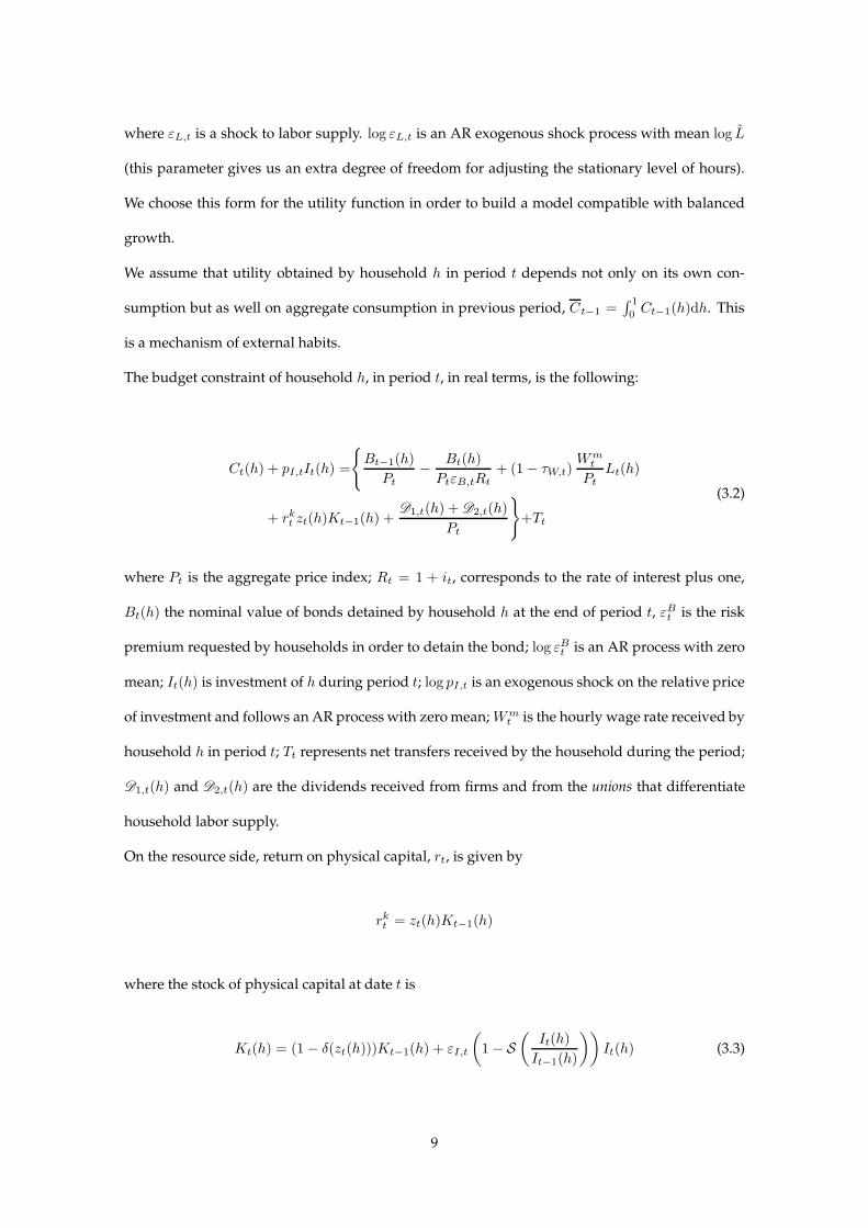
where εL,t is a shock to labor supply. log εL,t is an AR exogenous shock process with mean log L
(this parameter gives us an extra degree of freedom for adjusting the stationary level of hours).
We choose this form for the utility function in order to build a model compatible with balanced
growth.
We assume that utility obtained by household h in period t depends not only on its own con-
sumption but as well on aggregate consumption in previous period, Ct−1 =∫ 1
0 Ct−1(h)dh. This
is a mechanism of external habits.
The budget constraint of household h, in period t, in real terms, is the following:
Ct(h) + pI,tIt(h) =
Bt−1(h)
Pt−
Bt(h)
PtεB,tRt+ (1 − τW,t)
Wmt
PtLt(h)
+ rkt zt(h)Kt−1(h) +D1,t(h) + D2,t(h)
Pt
+Tt
(3.2)
where Pt is the aggregate price index; Rt = 1 + it, corresponds to the rate of interest plus one,
Bt(h) the nominal value of bonds detained by household h at the end of period t, εBt is the risk
premium requested by households in order to detain the bond; log εBt is an AR process with zero
mean; It(h) is investment of h during period t; log pI,t is an exogenous shock on the relative price
of investment and follows an AR process with zeromean;Wmt is the hourly wage rate received by
household h in period t; Tt represents net transfers received by the household during the period;
D1,t(h) and D2,t(h) are the dividends received from firms and from the unions that differentiate
household labor supply.
On the resource side, return on physical capital, rt, is given by
rkt = zt(h)Kt−1(h)
where the stock of physical capital at date t is
Kt(h) = (1 − δ(zt(h)))Kt−1(h) + εI,t
(1 − S
(It(h)
It−1(h)
))It(h) (3.3)
9

zt(h) ∈ [0, 1] is the rate of utilization of physical capital with steady value z⋆ ; the depreciation
rate, δ, is a function of the rate of utilization that verifies δ(0) = 0, δ(1) = 1, δ(z)′ > 0 for all
z ∈ [0, 1] and we write δ(z⋆) = δ⋆ ; εI,t is a random shock to the efficiency of capital accumulation
log εI,t is an AR process with zero mean; function S describes adjustment costs on investment, we
assume S(1 + g) = 0, where g is the rate of growth of investment on the balanced growth path,
furthermore S(1 + g)′ = 0 and S′′ > 0.
Each household h chooses its consumption, labor supply, bond holdings, investment, and capital
utilization rate so as to maximize its inter-temporal utility (3.1) under the budget constraint (3.2)
and the the law of evolution of physical captital (3.3), taking as given evolution of prices and
exogenous variables.
The first order optimality conditions are given by:
(Ct(h) − ηCt−1
)−σcexp
εL,t
σc − 1
1 + σlLt(h)
1+σl
= λt(h) (3.4)
where λt(h) is the Lagrange multiplier associated to the real budget constraint,
λt(h) = βεB,tRtEt
[λt+1(h)
πt+1
](3.5)
where πt+1 ≡ Pt+1/Pt is the inflation rate between period t and t+ 1,
ut(h) (σc − 1) εL,tLt(h)σl = −λt(h)
Wmt
Pt. (3.6)
Writing µt(h) the Lagrange multiplier associated to the capital accumulation function one gets:
pI,tλt(h) = µt(h)εI,t
[1 − S
(It(h)
It−1(h)
)−
It(h)
It−1(h)S′
(It(h)
It−1(h)
)]
+βEt
[µt+1(h)εI,t+1
(It+1(h)
It(h)
)2
S′
(It+1(h)
It(h)
)] (3.7)
µt(h)δ′ (zt(h)) = λt(h)r
kt (3.8)
10

and at last:
µt(h) = βEt
[µt+1(h)
(1 − δ(zt+1(h))
)+ λt+1(h)r
kt+1zt+1(h)
](3.9)
Given the symmetrical nature of the solution for the household’s problem, we get the following
aggregated relationships:
(Ct − ηCt−1)−σc exp
εL,t
σc − 1
1 + σlL1+σlt
= λt (3.10)
λt = βεB,tRtEt
[λt+1
πt+1
](3.11)
utεL,t (σc − 1)Lσlt = −λtWmt
Pt(3.12)
pI,tεI,t
= Qt
[1 − S
(ItIt−1
)−
ItIt−1
S′
(ItIt−1
)]+βEt
[λt+1
λtQt+1
εI,t+1
εI,t
(It+1
It
)2
S′
(It+1
It
)](3.13)
Qtδ′ (zt) = rkt (3.14)
Qt = βEt
[λt+1
λt
(Qt+1
(1 − δ(zt+1)
)+ rkt+1zt+1
)](3.15)
Here,Qt ≡ µt/λt is Tobin’s Q.
3.2 Production
3.2.1 Final good producers
Producers of final good, Yt, operate in a perfectly competitive environment, assembling a contin-
uum of diversified intermediary goods written Yt(ι) with ι ∈ [0, 1]. They have access to a unique
11

constant return aggregation technology as in Kimball [1996], implicitly defined by
∫ 1
0
Gf
(Yt(ι)
Yt
)dι = 1 (3.16)
where Gf is a strictly increasing concave function such that Gf(1) = 1. We follow Dotsey and King
[2005] or Levin et al. [2007] and adopt the following functional form for this aggregation function:
Gf(x) =θf (1 + ψf )
(1 + ψf )(θf (1 + ψf ) − 1)
[(1 + ψf
)x− ψf
] (1+ψf )θf−1
(1+ψf )θf −
[θf (1 + ψf )
(1 + ψf )(θf (1 + ψf ) − 1)− 1
]
(3.17)
Parameter ψf characterize the curvature of the demand function.
The producer of final good chooses the quantity of intermediary goods ι so as to maximize her
real profit:
Yt −
∫ 1
0
Pt(ι)
PtYt(ι)dι
under the technological constraints (3.16) and (3.17). As the aggregation function is homogeneous
of degree one, it is equivalent to minize cost per unit with respect to the relative demand of
intermediary good ι under the technological constraint.
The first order condition of optimality determines the demand for intermediary good ι:
Yt(ι)
Yt=
1
1 + ψf
[(Pt(ι)/Pt
Θt
)−(1+ψf )θf
+ ψf
](3.18)
whereΘt is the Lagrange multiplier associated with the technological constraints (3.16) and (3.17)
for the representative firm. Substituting (3.18) in the technological constraints, one gets the fol-
lowing expression for the Lagrange multiplier:
Θt =
(∫ 1
0
(Pt(ι)
Pt
)1−θf (1+ψf )
dι
) 11−θf (1+ψf )
(3.19)
12

The price elasticity of demand is given by:
ǫ(Yt(ι)
)= −
G ′(Yt(ι)
)
Yt(ι)G ′′(Yt(ι)
)
and, with particular aggregation function adpopted in this study,
ǫ(Yt(ι)
)= θf
[1 + ψf −
ψf
Yt(ι)
]
When ψf is equal to zero, we get back to the more usual case of the CES aggregator of Dixit-
Stiglitz Dixit and Stiglitz [1977] with a price elasticity of demand equal to θf . More generally, one
remarks that demand is more sensitive to price when the level of demand is important if and only
if parameter ψf is positive. We expect therefore to obtain a negative value for this parameter.
Finally, as the final good sector is perfectly competitive, profit for the representative firm must be
zero and we derive the aggregate price index:
Pt =ψf
1 + ψf
∫ 1
0
Pt(ι)dι +1
1 + ψf
(∫ 1
0
Pt(ι)1−(1+ψf )θfdι
) 11−(1+ψf )θf
(3.20)
3.2.2 Intermediary goods producers
A continuum of firms ι ∈ [0, 1] in monolistic competition produce intermediary goods for the
producers of the final good. These firms have all access to the same Cobb–Douglas technology in
to transform physical capital and labor in differentiated intermediary goods:
Yt(ι) =(Kdt (ι)
)α (AtL
dt (ι))1−α
(3.21)
where Kdt (ι) and L
dt (ι) are demands of intermediary good firm ι for physical capital, and labor,
respectively; At is technical progress, neutral in Harrod sense. The latter term is further decom-
13

posed in a trend component AT,t and a cyclical on AC,t. We have then,
∆logAT,t ∼ AR(1) stationary with mean log(1 + g) (3.22a)
logAC,t ∼ AR(1) stationary with zero mean. (3.22b)
Each intermediary firm ι ∈ [0, 1] buys freely its production factors on competitive markets taking
their price as given. The firm ι ∈ [0, 1] decides upon the mix of physical capital (Kdt (ι)) and labor
(Ldt (ι)) so as to minimize its cost, rktKdt (ι)+wtL
dt (ι), under the technological constraint (3.21). The
firm optimal behavior on the factor markets is summarized by the following factor prices frontier:
wtLdt (ι)
rktKdt (ι)
=1 − α
α(3.23)
where wt ≡ Wt/Pt is the real wage. The ratio of capital to labor is invariant across firms. Using
the factor prices frontier, we rewrite the total cost of firm ι as a function of the stock of capital:
CTt(ι) =rktK
dt (ι)
α
On the other hand, as the returns of scale is constant, we know that the total cost can also be
written as
CTt(ι) = mct(ι)Yt(ι)
where mct(ι) is the real marginal cost. We derive then the following expression for the marginal
cost of firm ι:
mct(ι) = Aα−1t
(rktα
)α(wt
1 − α
)1−α
≡ mct (3.24)
Again, marginal cost doesn’t depend on the size of the firm and is constant across firms.
14

The nominal profit of a firm that offers price P at date t id given by:
Πt(P) =
(εy,t
P
Pt−mct
)(P
Pt
)−(1+ψf )θf(∫ 1
0
(Pt(ι)
Pt
)1−(1+ψf )θf
df
) (1+ψf )θf1−(1+ψf )θf
+ ψf
PtYt1 + ψf
where log εy,t, an zero mean AR stationary process, is a shock to the sales of the firm.
Firm ι has market power but can’t decide of the its optimal price in each period. Following a
Calvo scheme, at each date, the firm receives a signal telling it whether it can revise its price Pt(ι)
in an optimal manner or not. There is a probability ξp that the firm can’t revise its price in a given
period. In such a case, the firm follows the following rule:
Pt(ι) = [πt]γp
[Pt−1
Pt−2
]1−γpPt−1(ι) = ΓtPt−1(ι) (3.25)
where πt si the inflation target of the monetary authorities. More generally, we write
Γt+j,t =
(j−1∏
h=0
πt+h
)γp (j−1∏
h=0
πt+h
)1−γp
= Γt+1Γt+2 . . .Γt+j
the growth factor of the price of a firm that doesn’t receive a favorable signal during j successive
periods(for j = 0 we have Γt,t = 1; for j = 1, we have Γt+1,t = Γt+1). When the firm ι receives a
positive signal (with probability 1 − ξp), it chooses price Pt(ι) that maximizes its profit.
Let Vt be the value of a firm that receives a positive signal in period t and Vt(Pt−1(ι)) the value
of a firm that receives a negative signal. As a firm that receives a negative signal follows simply
the ad hoc pricing rule (3.25), its value at time t depends only on Pt−1(ι). For a firm that receives
a positive signal, its value at period t is
Vt = maxP
Πt
(P
)+ βEt
[Λt+1
Λt
((1 − ξp)Vt+1 + ξpVt+1
(P))]
(3.26)
where Λt is the Lagrange multiplier of the budget constraint of the representative household and
PtΛt = λt. Let P⋆ be the optimal price choosen by the firm that can re–optimize.
15

The value of a firm that can’t re–optimize is
Vt(Pt−1(ι)
)= Πt
(ΓtPt−1(ι)
)+ βEt
[Λt+1
Λt
((1 − ξp)Vt+1 + ξpVt+1
(ΓtPt−1(ι)
))](3.27)
The first order condition and the envelope theorem give
Π′t
(P ⋆)
+ βξpEt
[Λt+1
ΛtV ′t+1
(P ⋆)]
= 0 (3.28a)
V ′t
(Pt−1(ι)
)
Γt= Π′
t
(ΓtPt−1(ι)
)+ βξpEt
[Λt+1
ΛtV ′t+1
(ΓtPt−1(ι)
)](3.28b)
with the derivative of profit at P :
Π′t
(P)
= εy,t1 − θf (1 + ψf )
1 + ψf
(P
Pt
)−(1+ψf )θf
Θ(1+ψf )θft Yt
+θf
(P
Pt
)−(1+ψf )θf−1
Θ(1+ψf )θft mctYt +
ψf1 + ψf
εy,tYt
(3.29)
Let’s write temporarily, in order to simplify notations, P , the price inherited from the past. One
can rewrite, one period ahead
V ′t+1
(P)
= Γt+1,tΠ′t+1
(Γt+1,tP
)+ βξpΓt+1,tEt+1
[Λt+2
Λt+1V ′t+2
(Γt+1,tP
)]
Iterating toward the future and applying conditional expectation at time t, one gets
Et
[V ′t+1
(P)]
= Et
∞∑
j=0
(βξp)jΓt+1+j,t
Λt+1+j
Λt+1Π′t+1+j
(Γt+1+j,tP
)
By substitution ( P = P ⋆) inf the first order condition, one gets the following condition for the
price choosen by the firm that gets a positive signal:
Et
∞∑
j=0
(βξp)jΓt+j,t
Λt+jΛt
Π′t+j
(Γt+j,tP
⋆t
) = 0 (3.30)
One can get a more explicit expression for the price that satisfies equation (3.30). Substituting in
16

this equation the expression of marginal profit (3.29) and dividing by P ⋆t−(1+ψf )θf one gets:
P ⋆tPt
=θf (1 + ψf )
θf (1 + ψf ) − 1
Z1,t
Z2,t+
ψfθf (1 + ψf ) − 1
(P ⋆tPt
)1+(1+ψf )θfZ3,t
Z2,t(3.31)
with
Z1,t = Et
∞∑
i=0
(βξp)jλt+j
(Γt+jPt+j/Pt
)−(1+ψf )θf
Θ(1+ψf )θft+j mct+jYt+j (3.32a)
Z2,t = Et
∞∑
i=0
(βξp)jλt+jεy,t+j
(Γt+jPt+j/Pt
)1−(1+ψf )θf
Θ(1+ψf )θft+j Yt+j (3.32b)
Z3,t = Et
∞∑
i=0
(βξp)jλt+jεy,t+j
Γt+jPt+j/Pt
Yt+j (3.32c)
writing Pt+j/Pt, the inflation factor between t and t+ j, can be written equivalently Πji=1πt+i, and
we can represent variables Z1,t, Z2,t et Z3,t in recursive form:
Z1,t = λtmctΘ(1+ψf )θft Yt + βξpEt
(
πt+1
πγpt−1π
1−γpt
)(1+ψf )θf
Z1,t+1
(3.33a)
Z2,t = λtεy,tΘ(1+ψf )θft Yt + βξpEt
(
πt+1
πγpt−1π
1−γpt
)(1+ψf )θf−1
Z2,t+1
(3.33b)
Z3,t = λtεy,tYt + βξpEt
[(πγpt−1π
1−γpt
πt+1
)Z3,t+1
](3.33c)
Writing ϑf,t ≡∫ 1
0Pt(ι)Pt
dι can be written in recursive form:
ϑf,t = (1 − ξp)P ⋆tPt
+ ξpπ
1−γpt π
γpt−1
πtϑf,t−1 (3.34)
we can finally write the equation (3.20) equaivalently as:
ψfϑf,t1 + ψf
+Θt
1 + ψf= 1 (3.35)
17

In the end, inflation dynamics are characterized by equations (3.35), (3.34), (3.31), (3.33a), (3.33b),
(3.33c).
3.3 Labor
Homogeneous labor Lt =∫ 1
0 Lt(h)dh provided by the households is differentiated by a contin-
uum of unions, ς ∈ [0, 1]. We have then Lt =∫ 1
0 lt(ς)dς . Unions sell differentiated labor, lt(ς),
to an employment agency that aggregate different types of labor to offer it as input to the firms
of the intermediary good sector. Unions have monopolistic power and the employment agency
operates in a perfectly competitive manner.
3.3.1 Employment agency
It aggregates lagor lt(ς) provided by unions with an aggregation function as in Kimball [1996],
defined implicitly by∫ 1
0
Gs
(lt(ς)
Lt
)dς = 1 (3.36)
where Gs is a strictly increasing concave function such that Gs(1) = 1. We use the following
specification:
Gs(x) =θs(1 + ψs)
(1 + ψs)(θs(1 + ψs) − 1)
[(1 + ψs
)x− ψs
] (1+ψs)θs−1(1+ψs)θs
−
[θs(1 + ψs)
(1 + ψs)(θs(1 + ψs) − 1)− 1
]
(3.37)
This function is a generalization of the Dixit–Stiglitz aggregator Dixit and Stiglitz [1977] that is
a particular case when ψs = 0. The employment agency chooses the relative quantity of labor
of type ς such as minimizing the cost of production by unit of homogenous labor, Wt(ς)Wt
lt(ς)Lt
,
under the technological constraints (3.36) and (3.37). The first order condition associated to the
optimization program of the employment agency determines its demand of differentiated labor3
ς :
lt(ς)
Lt=
1
1 + ψs
[(Wt(ς)/Wt
Υt
)−(1+ψs)θs
+ ψs
](3.38)
3In order to save in notations, we don’t make a difference between the demand of the employment agency and thesupply by the unions.
18
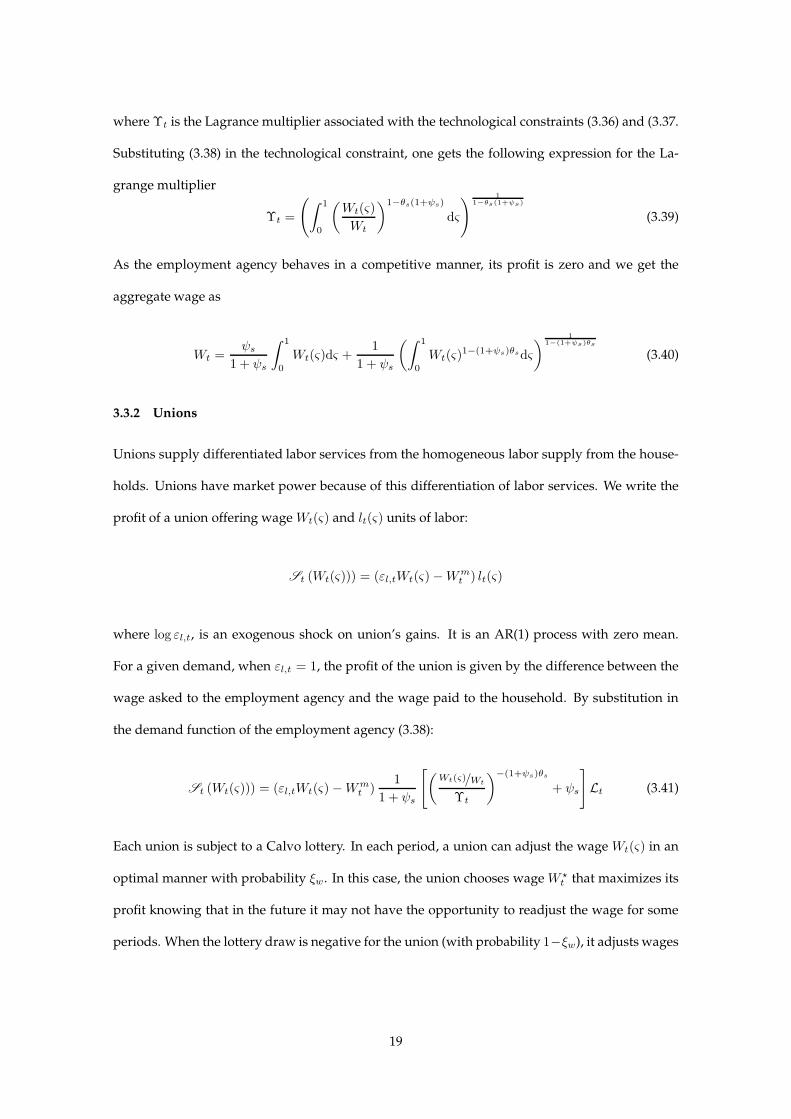
where Υt is the Lagrance multiplier associated with the technological constraints (3.36) and (3.37.
Substituting (3.38) in the technological constraint, one gets the following expression for the La-
grange multiplier
Υt =
(∫ 1
0
(Wt(ς)
Wt
)1−θs(1+ψs)
dς
) 11−θs(1+ψs)
(3.39)
As the employment agency behaves in a competitive manner, its profit is zero and we get the
aggregate wage as
Wt =ψs
1 + ψs
∫ 1
0
Wt(ς)dς +1
1 + ψs
(∫ 1
0
Wt(ς)1−(1+ψs)θsdς
) 11−(1+ψs)θs
(3.40)
3.3.2 Unions
Unions supply differentiated labor services from the homogeneous labor supply from the house-
holds. Unions have market power because of this differentiation of labor services. We write the
profit of a union offering wageWt(ς) and lt(ς) units of labor:
St (Wt(ς))) = (εl,tWt(ς) −Wmt ) lt(ς)
where log εl,t, is an exogenous shock on union’s gains. It is an AR(1) process with zero mean.
For a given demand, when εl,t = 1, the profit of the union is given by the difference between the
wage asked to the employment agency and the wage paid to the household. By substitution in
the demand function of the employment agency (3.38):
St (Wt(ς))) = (εl,tWt(ς) −Wmt )
1
1 + ψs
[(Wt(ς)/Wt
Υt
)−(1+ψs)θs
+ ψs
]Lt (3.41)
Each union is subject to a Calvo lottery. In each period, a union can adjust the wageWt(ς) in an
optimal manner with probability ξw. In this case, the union chooses wageW ⋆t that maximizes its
profit knowing that in the future it may not have the opportunity to readjust the wage for some
periods. When the lottery draw is negative for the union (with probability 1−ξw), it adjusts wages
19

according to the following ad hoc rule:
Wt(ς) =AT,t
AT,t−1πγwt−1π
1−γwt−1 Wt−1(ς) (3.42)
We write Ωt = (AT,t/AT,t−1) πγwt−1π
1−γwt−1 ≡ Ωt,t−1 the growth factor of nominal wage asked by the
union ς at date t when this one doesn’t have the opportunity of revising it in an optimal manner.
In this case, the union changes the wage by indexing it on (i) a convex mix of the inflation target
of the monetary authority and of past inflation and (ii) the efficiency growth in the intermediary
goods sector. We write
Ωt+j,t =AT,t+j
AT,t
(j−1∏
h=0
πt+h
)γw (j−1∏
h=0
πt+h
)1−γw
= Ωt+1Ωt+2 . . .Ωt+j
the growth factor of the wage of a a union that gets negative signals during the the next j periods
(for j = 0, we have Ωt,t = 1, for j = 1, we have Ωt+1,t = Ωt+1).
Let Ut be the value of a union that receives a positive signal at date t and Ut(Wt−1(ς)) the value
of a union that receives the negative signal. In the latter case, the union follows simply the ad
hoc rule (3.42), this explains why its value at date t depends upon Wt−1(ς). On the opposite, the
optimization program of a union that receives a positive signal is purely turn towards the future.
As unions have the same expectations about the future, they all choose the same optimal wage
(W ⋆t ). More formally, the value at date t of a union that receives a positive signal is
Ut = maxW
St
(W
)+ βEt
[Λt+1
Λt
((1 − ξw)Ut+1 + ξwUt+1
(W))]
(3.43)
where Λt is the Lagrange multiplier associated to the nominal budget constraint of the represen-
tative household.
The value of a union that receives a negative signal is
Ut(Wt−1(ς)
)= St
(ΓtWt−1(ς)
)+ βEt
[Λt+1
Λt
((1 − ξw)Ut+1 + ξwUt+1
(ΓtWt−1(ς)
))](3.44)
20

The first order condition and the application of the envelop theorem give
S′t
(W ⋆t
)+ βξwEt
[Λt+1
ΛtU ′t+1
(W ⋆t
)]= 0 (3.45a)
U ′t
(Wt−1(ς)
)
Γt= S
′t
(ΓtWt−1(ς)
)+ βξpEt
[Λt+1
ΛtU ′t+1
(ΓtWt−1(ς)
)](3.45b)
with the derivative of the union profit atW :
S′t
(W)
= εl,t1 − θs(1 + ψs)
1 + ψs
(W
Wt
)−(1+ψs)θs
Υ(1+ψs)θst Lt
+θs
(W
Wt
)−(1+ψs)θs−1
Υ(1+ψs)θst
Wmt
Wt
Lt +ψs
1 + ψsεl,tLt
(3.46)
Let’s write temporarily, in order to simplify notations, W , the price inherited from the past. One
can rewrite, one period ahead
U ′t+1
(W)
= Ωt+1,tS′t+1
(Ωt+1,tW
)+ βξpΩt+1,tEt+1
[Λt+2
Λt+1U ′t+2
(Ωt+1,tW
)]
iterating toward the future and applying conditional expectation gives
Et
[U ′t+1
(W)]
= Et
∞∑
j=0
(βξp)jΩt+1+j,t
Λt+1+j
Λt+1S
′t+1+j
(Ωt+1+j,tW
)
Substituting in the first order condition (pour W = W ⋆t ), one gets the following condition for an
optimal wage choice by a union that receives a positive signal:
Et
∞∑
j=0
(βξp)jΩt+j,t
Λt+jΛt
S′t+j
(Ωt+j,tW
⋆t
) = 0 (3.47)
The optimal wageW ⋆t is the nominal wage that insures that the sum of current and expected dis-
counted marginal profits are zero when the union can only revise nominal wages by using the ad
hoc rule (3.42).
21

It is possible to obtain a recursive expression for multiplier Υt that appears in the expression for
a union profit. Equation (3.39) can be written equivalently in the form
Υ1−θs(1+ψs)t =
∫ 1
0
(Wt(ς)
Wt
)1−θs(1+ψs)
dς
The wage offered by the union at date t appears under the integral sign. This price has been
determined optimaly j periods beforewith probability (1−ξw)ξjw . We can then rewrite the integral
as
Υ1−θs(1+ψs)t = (1 − ξw)
∞∑
j=0
ξjw
(Ωt,t−jW
⋆t−j
Wt
)1−θs(1+ψs)
where W ⋆t−j is the optimal wage at date t − j. Finally, one can interpret the infinite sum as the
solution of the following recursive equation:
Υ1−θs(1+ψs)t = (1 − ξw)
(W ⋆t
Wt
)1−θs(1+ψs)
+ ξw
(Ωt,t−1
Wt/Wt−1
)1−θs(1+ψs)
Υ1−θs(1+ψs)t−1 (3.48)
One can get a more explicit expression for the wage that satisfies equation (3.47). Substituting in
this equation the expression for marginal profit (3.46) and dividing by W ⋆t
−(1+ψs)θs , one gets
w⋆twt
=θs(1 + ψs)
θs(1 + ψs) − 1
H1,t
H2,t+
ψsθs(1 + ψs) − 1
(w⋆twt
)1+(1+ψs)θsH3,t
H2,t(3.49)
where w⋆t is the real wage obtained by the union at date t when it can adjust the nominal wage in
an optimal manner and wt the real nominal wage in the economy, with
H1,t = Et
∞∑
i=0
(βξw)jλt+jwmt+j
(Ωt+j
wt+jwt
Pt+jPt
)−(1+ψs)θs
Υ(1+ψs)θst+j Lt+j (3.50a)
H2,t = Et
∞∑
i=0
(βξw)jλt+jεl,t+jwt+j
(Ωt+j
wt+jwt
Pt+jPt
)1−(1+ψs)θs
Υ(1+ψs)θst+j Lt+j (3.50b)
H3,t = Et
∞∑
i=0
(βξw)jλt+jεl,t+jwt+jΩt+j
wt+jwt
Pt+jPt
Lt+j (3.50c)
22

Noticing that wt+j/wt, the growth factor of the real wage between t and t+ j, can be equivalently
written as Πji=1t+i (t is the growth factor of the real wage between t and t − 1) and that we
have
Ωt+j,t = (1 + g)j
(j∏
h=1
Et+h
) 11−ρx
(j−1∏
h=0
πt+h
)γw (j−1∏
h=0
πt+h
)1−γw
,
we can finally represent variables H1,t, H2,t and H3,t in the recursive form
H1,t = λtwmt LtΥ
(1+ψs)θst + βξwEt
t+1πt+1
(1 + g)E1
1−ρxt+1 πγwt−1π
1−γwt
(1+ψs)θs
H1,t+1
(3.51a)
H2,t = λtεl,twtLtΥ(1+ψs)θst + βξwEt
t+1πt+1
(1 + g)E1
1−ρxt+1 πγwt−1π
1−γwt
(1+ψs)θs−1
H2,t+1
(3.51b)
H3,t = λtεl,twtLt + βξwEt
(1 + g)E
11−ρxt+1 πγwt−1π
1−γwt
t+1πt+1
H3,t+1
(3.51c)
Noticing that ϑs,t ≡∫ 1
0Wt(ς)Wt
dς can be written in the recursive form
ϑs,t = (1 − ξw)w⋆twt
+ ξw(1 + g)E
11−ρxt πγwt−1π
1−γwt
tπtϑs,t−1 (3.52)
we can rewrite equation (3.40) as
ψsϑs,t1 + ψs
+Υt
1 + ψs= 1 (3.53)
In the end, wage dynamics are characterized by equations (3.45), (3.52), (3.48), (3.49), (3.51a),
(3.51b), (3.51c).
3.4 Government and monetary authority
3.4.1 Fiscal policy
We assume that exogenous government expenditures Gt = gtYt are exactly financed by lump
sum taxes:
Tt = PtGt.
23

3.4.2 Central Bank
We assume that the behavior of the central bank is adequately described by a simple Taylor rule:
Rt = RρRt−1
[R⋆(πt−1
πt
)rπ ( YtYt
)rY ]1−ρRεR,t (3.54)
where πt is the inflation target of the central bank, Yt is a reference output level to be defined
later, log εR,t is an AR(1) stationary process with zero mean.
3.5 General equilibrium
3.5.1 Price distortion
Prices in the intermediary good sector are heterogeneous. However, it is possible to show that
this heterogeneity doesn’t hinder aggregation. We know that the firms of this sector choose all
the same mix of factor of production in the sense that the ratio of capital demand to labor demand
is constant across firms (see equation 3.23). Expressing labor demand of firm ι as a function of its
demand of physical capital, we can write the production of this firm
yt(ι) =
(AtL
dt
Kdt
)1−α
Kdt (ι)
When Kdt ≡
∫ 1
0Kdt (ι)dι is aggregate demand for physical capital and yt ≡
∫ 1
0Yt(ι)dι represents
the sum of intermediary productions, we can write directly
yt =(Kdt
)α (AtL
dt
)1−α
The sum of intermediary productions is different from Yt, because aggregation technology isn’t
linear. Integrating the demand function for good ι from the final good producers (3.18) over ι, we
get
yt = ∆p,tYt (3.55)
24

with
∆p,t ≡1
1 + ψf
∫ 1
0
((Pt(ι)/Pt
Θt
)−(1+ψf )θf
+ ψf
)dι (3.56)
Price distortion can be written recursively in the following manner:
∆p,t =1
1 + ψfΘ
(1+ψf )θft ∇p,t +
ψf1 + ψf
(3.57a)
∇p,t = (1 − ξp)
(P ⋆tPt
)−(1+ψf )θf
+ ξp
(πγpt π
1−γpt−1
πt
)−(1+ψf )θf
∇p,t−1 (3.57b)
where the Lagrange multiplier Θt is defined recursively as well. Then, we have
∆p,tYt =(Kdt
)α (AtL
dt
)1−α(3.58)
3.5.2 Wage distortion
Here, we show how to link aggregate labor supply by the households with aggregated labor sup-
ply by the employment agency to the firms of the intermediary good sector This link is affected
by the heterogeneity of wages induced by their nominal rigidity. Integrating labor demand for
type ς by the employment agency (3.38) over ς , we find directly
Lt = ∆w,tLt (3.59)
with
∆w,t ≡1
1 + ψs
∫ 1
0
((Wt(ς)/Wt
Υt
)−(1+ψs)θs
+ ψs
)dς (3.60)
Wage distortion can be written in recursive form:
∆w,t =1
1 + ψsΥ
(1+ψs)θst ∇w,t +
ψs1 + ψs
(3.61a)
25

∇w,t = (1 − ξw)
(w⋆twt
)−(1+ψs)θs
+ ξs
(1 + g)E
11−ρxt πγwt π1−γw
t−1
tπt
−(1+ψs)θs
∇w,t−1 (3.61b)
where the Lagrange multiplier Υt is defined recursively in equation (3.48).
3.5.3 Dividends paid by intermediary good firms
Firms in the intermediary good sector interact in monopolistic competition and make profits that
are paid to households in the form of dividends. The sum of nominal profits at date t is
Πt =
∫ 1
0
Πt(ι)dι
=
∫ 1
0
(εy,t
Pt(ι)
Pt−mct
)PtYt(ι)dι
= εy,t
∫ 1
0
Pt(ι)Yt(ι)dι − Ptmctyt
= εy,tPtYt −
(Ptr
kt
∫ 1
0
Kdt (ι)dι +Wt
∫ 1
0
Ldt (ι)dι
)
= Pt(εy,tYt − rktK
dt − wtL
dt
)
As households own the firms, the profits are paid to them. The repartition of these profits between
the households in undetermined in general equilibrium, but we know that
∫ 1
0
D1,t(h)dh = Pt(εy,tYt − rktK
dt − wtL
dt
)(3.62)
3.5.4 Dividends paid by the unions
In the same way, we can compute aggregate nominal profit of the unions at date t. These profits
as well are paid to the households. We have
St =
∫ 1
0
St(ς)dς
=
∫ 1
0
(εl,tWt(ι) −Wmt ) lt(ς)dς
= εl,t
∫ 1
0
Wt(ς)lt(ς)dς −Wmt Lt
= εl,tWtLt −Wmt Lt
26

and, then,∫ 1
0
D2,t(h)dh = εl,tWtLt −Wmt Lt (3.63)
3.5.5 Equilibrium in factor markets and in bond markets
In general equilibrium, labor supply form the employment agency equals aggregate labor de-
mand by firms of the intermediary good market. In the same way, aggregate supply of physical
capital by the households equals aggregate demand from these firms. In formal terms,
Lt ≡ ∆−1w,t
∫ 1
0
Lt(h)dh =
∫ 1
0
Ldt (ι)dι ≡ Ldt (3.64)
Kt ≡
∫ 1
0
zt(h)Kt−1(h)dh =
∫ 1
0
Kdt (ι)dι ≡ Kd
t (3.65)
Finally, aggregate demand for bonds must be zero, as we assume a close economy and no gov-
ernment debt.∫ 1
0
Bt(h)dh = 0 (3.66)
3.5.6 Equilibrium on the good market
By summing the budget constraints of the households (3.2) over h ∈ [0, 1] and by substituting the
equilibrium conditions on the bond market, the definition of aggregate dividends and the budget
constraint of the government, we get
PtGt + PtCt + pI,tPtIt = Wmt Lt + Ptr
Kt ztKt−1 + Pt
(εy,tYt − rktK
dt − wtL
dt
)
+ εltWtLt −Wmt Lt
After simplification and knowing that the factor markets are in equilibrium, we obtain
Gt + Ct + pI,tIt = εy,tYt + (εl,t − 1)wtLt (3.67a)
27

or equivalently
Gt + Ct + pI,tIt = εy,t∆−1p,tyt + (εl,t − 1)∆−1
w,twtLt (3.67b)
3.6 Long run
The economy described in the model is growing at a constant rate in the long run, in absence of
shocks. In order to compute a local approximation in order to solve it and later to estimate it, we
need first to make it stationary.
In this model, there is a single source of growth in the long run: the Harrodian technical change
that is characterized by a stochastic trend (with a deterministic component) and affects most of
the real variables. In order to stationarize the model, we divide all non–stationary variables by
AT,t or a power of this variable. In this section we present the stationarized model and then its
stationary state.
3.6.1 Stationary version of the model
On the household side, we write Ct ≡ CtAT,t, λt = λtA−σcT,t , w
mt = wmt AT,t, It ≡ ItAT,t. In order
to make estimation (or calibration) of the long run level of εL,t (ie the scale factor that lets obtain
the desired long run level for labor hours), we redefine the utility function, replacing Lt by Lt/L
where L is the long run level of labor hours.
(Ct − η
AT,t−1
AT,t
Ct−1
)−σc
exp
εL,t
σc − 1
1 + σl
(LtL
)1+σl
= λt (3.68)
λt = βεB,tRtEt
[(AT,t+1
AT,t
)−σc λt+1
πt+1
](3.69)
[Ct − η
AT,t−1
AT,t
Ct−1
]1−σc εL,tL
exp
εL,t
σc − 1
1 + σl
(LtL
)1+σl(
LtL
)σl= λtw
mt (3.70)
28

pI,tεI,t
= Qt
[1 − S
(It
It−1
AT,t
AT,t−1
)−
It
It−1
AT,t
AT,t−1S′
(It
It−1
AT,t
AT,t−1
)]
+ βEt
λt+1
λt
(AT,t+1
AT,t
)−σc
Qt+1εI,t+1
εI,t
(It+1
It
AT,t+1
AT,t
)2
S′
(It+1
It
AT,t+1
AT,t
)
(3.71)
Qtδ′ (zt) = rkt (3.72)
Qt = βEt
[λt+1
λt
(AT,t+1
AT,t
)−σc (Qt+1
(1 − δ(zt+1)
)+ rkt+1zt+1
)](3.73)
Notice that Tobin’s Q Qt is a stationary variable. Therefore, by its definition, the Lagrange multi-
plier µt is trended. We write µt = µtAσcT,t.
LetKt ≡ KtAT,t, and the dynamics for the stock of capital is
Kt = (1 − δ(zt))AT,t−1
AT,t
Kt−1 + εI,t
(1 − S
(It
It−1
AT,t
AT,t−1
))It (3.74)
On the production side, the factor price frontier becomes
wtLdt
rkt Kdt
=1 − α
α. (3.75)
Marginal cost is written
mct = Aα−1C,t
(rktα
)α(wt
1 − α
)1−α
(3.76)
For the price equations, we define Zi,t = Zi,tA1−σcT,t for i = 1, 2 and 3, then,
P ⋆tPt
=θf (1 + ψf )
θf (1 + ψf ) − 1
Z1,t
Z2,t
+ψf
θf (1 + ψf ) − 1
(P ⋆tPt
)1+(1+ψf )θfZ3,t
Z2,t
(3.77)
and
Z1,t = λtmctΘ(1+ψf )θft Yt + βξpEt
(AT,t+1
AT,t
)1−σc(
πt+1
πγpt−1π
1−γpt
)(1+ψf )θf
Z1,t+1
(3.78a)
29

Z2,t = λtεy,tΘ(1+ψf )θft Yt + βξpEt
(AT,t+1
AT,t
)1−σc(
πt+1
πγpt−1π
1−γpt
)(1+ψf )θf−1
Z2,t+1
(3.78b)
Z3,t = λtεy,tYt + βξpEt
[(AT,t+1
AT,t
)1−σc(πγpt−1π
1−γpt
πt+1
)Z3,t+1
](3.78c)
Equations (3.34) and (3.35) are unchanged.
For the unions and the employment agency, we define Hi,t = Hi,tA1−σcT,t for i = 1, 2 and 3,
w⋆t = AT,tw⋆t and t = tAT,t/AT,t−1. The relative wage of a union that has the possibility
to reoptimize in period t is
w⋆twt
=θs(1 + ψs)
θs(1 + ψs) − 1
H1,t
H2,t
+ψs
θs(1 + ψs) − 1
(w⋆twt
)1+(1+ψs)θsH3,t
H2,t
(3.79)
H1,t = λtwmt LtΥ
(1+ψs)θst + βξwEt
[(AT,t+1
AT,t
)1−σc ( t+1πt+1
πγwt π1−γwt
)(1+ψs)θs
H1,t+1
](3.80a)
H2,t = λtεl,twtLtΥ(1+ψs)θst + βξwEt
[(AT,t+1
AT,t
)1−σc ( t+1πt+1
πγwt π1−γwt
)(1+ψs)θs−1
H2,t+1
](3.80b)
H3,t = λtεl,twtLt + βξwEt
[(AT,t+1
AT,t
)1−σc(πγwt π1−γw
t
t+1πt+1
)H3,t+1
](3.80c)
ϑs,t can be expressed as a function of stationarized wages:
ϑs,t = (1 − ξw)w⋆twt
+ ξwπγwt π1−γw
t−1
tπtϑs,t−1 (3.81)
Equation (3.53) remains unchanged. Finally, wage distortion is expressed as a function of station-
arized wages:
∇w,t = (1 − ξw)
(w⋆twt
)−(1+ψs)θs
+ ξw
(πγwt π1−γw
t−1
tπt
)−(1+ψs)θs
∇w,t−1 (3.82)
Equilibrium conditions on the good and factor markets are the same for the stationarized vari-
30

ables.
3.6.2 Stationary state
At the stationary state, we have
(C −
η
1 + gC
)−σc
exp
Lσc − 1
1 + σl
= λ (3.83)
λ = βR(1 + g)−σcλ
π⋆(3.84)
[C −
η
1 + gC
]1−σc LL
exp
Lσc − 1
1 + σl
= λwm (3.85)
Q = 1 (3.86)
δ′ (z) = rk (3.87)
1 = β(1 + g)−σc(1 − δ + rkz
)(3.88)
K =1 + g
g + δI (3.89)
wLd
rkKd=
1 − α
α(3.90)
mc =
(rk
α
)α (w
1 − α
)1−α
(3.91)
31

P ⋆
P=
θf (1 + ψf )
θf (1 + ψf ) − 1
Z1
Z2
+ψf
θf (1 + ψf ) − 1
(P ⋆
P
)1+(1+ψf )θfZ3
Z2
(3.92)
Z1 = λmcΘ(1+ψf )θf Y + βξp(1 + g)1−σcZ1 (3.93a)
Z2 = λΘ(1+ψf )θf Y + βξp(1 + g)1−σcZ2 (3.93b)
Z3 = λY + βξp(1 + g)1−σcZ3 (3.93c)
ϑf =P ⋆
P(3.94)
ψfϑf1 + ψf
+Θ
1 + ψf= 1 (3.95)
∆p =1
1 + ψfΘ(1+ψf )θf∇p +
ψf1 + ψf
(3.96a)
∇p =
(P ⋆tPt
)−(1+ψf )θf
(3.96b)
Θ =P ⋆
P(3.97)
w⋆
w=
θs(1 + ψs)
θs(1 + ψs) − 1
H1
H2
+ψs
θs(1 + ψs) − 1
(w⋆
w
)1+(1+ψs)θsH3
H2
(3.98)
H1 = λwmLΥ(1+ψs)θs + βξw(1 + g)1−σcH1 (3.99a)
32

H2 = λwLΥ(1+ψs)θs + βξw(1 + g)1−σcH2 (3.99b)
H3 = λwL + βξw(1 + g)1−σcH3 (3.99c)
ϑs =w⋆
w(3.100)
ψsϑs1 + ψs
+Υ
1 + ψs= 1 (3.101)
∆w =1
1 + ψsΥ(1+ψs)θs∇w +
ψs1 + ψs
(3.102a)
∇w =
(w⋆
w
)−(1+ψs)θs
(3.102b)
Υ = 1 (3.103)
R = R⋆ (3.104)
∆pY =(Kd)α (
Ld)1−α
(3.105)
L = ∆wL (3.106)
Ld = ∆wL (3.107)
33

z
1 + gK = Kd (3.108)
C + I = (1 − g⋆) Y (3.109)
We can write equations (3.93a) to (3.93c) equivalently as
Z1 =λmcΘ(1+ψf )θf Y
1 − βξp(1 + g)1−σc(3.110a)
Z2 =λΘ(1+ψf )θf Y
1 − βξp(1 + g)1−σc(3.110b)
Z3 =λY
1 − βξp(1 + g)1−σc(3.110c)
Substituting in (3.92), we get
P ⋆
P=
θf (1 + ψf )
θf (1 + ψf ) − 1mc+
ψfθf (1 + ψf ) − 1
(P ⋆
P
)1+(1+ψf )θf
Θ−(1+ψf )θf (3.111)
that implicitly define real marginal cost at the stationary state as a function of optimal relative
price P⋆/P and the Lagrange multiplier from the optimization program for the firm that produces
the homogeneous good. Furthermore, sustitution equation (3.97) in (3.95), (3.94), (3.96b) and
(3.96a) we get
Θ = ϑf =P ⋆
P= ∇p = ∆p = 1 (3.112)
Marginal cost at the stationary state is then
mc =θf (1 + ψf ) − 1
θf (1 + ψf )−
ψfθf (1 + ψf )
=θf − 1
θf(3.113)
34

Finally, substituting (3.97) in equations (3.110a) to (3.110c) we obtain
Z1 = mcλY
1 − βξp(1 + g)1−σc(3.114a)
Z2 = Z3 = Z1/mc (3.114b)
where λ, Y are determined below iwth the other real variables.
We can write equations (3.99a) à (3.99c) in the following manner:
H1 =λwmLΥ(1+ψs)θs
1 − βξw(1 + g)1−σc(3.115a)
H2 =λwLΥ(1+ψs)θs
1 − βξw(1 + g)1−σc(3.115b)
H3 =λwL
1 − βξw(1 + g)1−σc(3.115c)
Substituting in (3.98) we get
w⋆
w=
θs(1 + ψs)
θs(1 + ψs) − 1
wm
w+
ψsθs(1 + ψs) − 1
(w⋆
w
)1+(1+ψs)θs
Υ−(1+ψs)θs (3.116)
that implicitly defines the ratio of real wage received by the household to the real wage paid to the
employment agency as a function of optimal real relative wage, bw⋆/bw, and the Lagrangemultiplier
from the optimization program of the employment agency.
Substituting equation (3.103) in equations (3.101), (3.100), (3.102b) and (3.102a) we obtain
Υ = ϑs =w⋆
w= ∇w = ∆w = 1 (3.117)
35

Then, we have
wm
w=θs(1 + ψs) − 1
θs(1 + ψs)−
ψsθs(1 + ψs)
(3.118)
Finally, subsituting (3.103) in (3.115a) to (3.115c) we get
H1 = wmλL
1 − βξw(1 + g)1−σc(3.119a)
H2 = H3 = H1w
wm(3.119b)
Equations (3.104) and (3.84) imply
R⋆ =π⋆
β(1 + g)σc (3.120)
In practive, we are estimating (or calibrating) R⋆ and π⋆ then we deduce β conditionally to the
current estimation of the growth rate along the balanced growth path, g. From equation (3.88) we
get the return on capital at the steady state:
rk =(1 + g)σc − β(1 − δ)
βz(3.121)
where δ et z are estimated (or calibrated). Equation (3.87) establishes the following constraints on
the derivative of the depreciation function at the steady state
δ′ (z) =(1 + g)σc − β(1 − δ)
βz(3.122)
Conditionally to the long run level of real marginal cost et return on capital, we obtain steady
state for the average real wage (relative to labor efficiency trend) using equation (3.91):
w =[mc( αrk
)α] 11−α
(1 − α) (3.123)
Along the balanced growth path, real wage growth rate is the same as the growth rate of labor
36

efficiency:
= 1 + g (3.124)
Substituting (3.123) in (3.113) we obtain the real wage received by the household (still normalized
by labor efficiency trend) at the steady state:
wm =
(θs(1 + ψs) − 1
θs(1 + ψs)−
ψsθs(1 + ψs)
)[mc( αrk
)α] 11−α
(1 − α) (3.125)
As price and wage distortion is zero at the steady state, we get
Ld = L = L (3.126)
and
Y = y =(Kd)α (
Ld)1−α
(3.127)
In what follows, we write χX,Y the ratio of two variables X and Y . Equation (3.90) and (3.126)
gives the capital labor ratio at the steady state:
χ bKd,L=w
rkα
1 − α(3.128)
Using equations (3.126), (3.127) and (3.128) it follows that product per capita at the steady state is
χbY ,L= χαbKd,L
(3.129)
On writes the equilibrium on the final good market (3.109) as
χ bC,bY+ χbI,bY
= 1 − g⋆ (3.130)
Using the equilibrium condition on the market for capital (3.108) as well as equations (3.128),
37

(3.129) and (3.89), one gets the share of investment in output at the steady state:
χbI,bY=g + δ
zχ1−α
bKd,L(3.131)
We can then determine χ bC,bYby complementarity, using equation (3.130). Dividing (3.85) by (3.83)
one gets(C −
η
1 + gC
)L
L= wm
Multiplying and dividing the left handside by Y , one gets
χ bC,bYχbY ,L
(1 −
η
1 + g
)L = wm
and then
L =wm
χ bC,bYχbY ,L
1 + g
1 + g − η(3.132)
Then,
Y = χbY ,LL (3.133)
C = χ bC,bYY (3.134)
I = χbI,bYY (3.135)
Finally, the steady state of the Lagrange multiplier associated with the household budget con-
straint is obtained from equation (3.83):
λ =
(C −
η
1 + gC
)−σc
exp
L
1 − σc1 + σl
(3.136)
38

3.7 Specifying functional forms
3.7.1 The depreciation function
The rate of depreciation of physical capital depends on the utilization rate of capital. This function
must verify δ(0) = 0 and δ(z)′ > 0 for any z ∈ [0, 1] and we write δ(z) = δ. We use the following
functional form:
δ(z) = δeδ′
δ(z−z) (3.137)
where δ′ ≡ δ′(z) is the first derivative of the rate of depreciation evaluated at the steady state.
This parameter is linked to parameters g, σc, β, δ and z thru equation (3.122) :
δ′ =(1 + g)σc − β(1 − δ)
βz> 0
This parameter should therefore be estimated or calibrated. An alternative to calibrate (or esti-
mate) δ is to calibrate (or estimate) the ratio χbI,bY. One can show that
δ =
θfχbI, bY
αβ(θf−1) (1 + g)σc −θfχbI, bY
α(θf−1) − g
1 −θfχbI, bY
α(θf−1)
It is possible to examine the data in order to form a prior on χbI,bY. It is a flexible way of exploiting
information about the relation between production and investment in the long run.
3.7.2 The investment adjustment cost function
Adjusting its investment level is costly for the household. This cost is described by function S.
One assumes that the cost is zero along the balance growth path, S(1 + g) = 0, that S(1)′ = 0, and
the cost is convex,t S′′ > 0. We choose the following specification form:
S(x) ≡ψ
2(x− (1 + g))2 (3.138)
where x ≡ It/It−1 is the growth factor for investment and ψ a parameter, real and positive, mea-
suring the size of adjusmtent costs. It needs to be calibrated or estimated. We can then express
39

the stationarized adjustment cost function for investment as
S
(It
It−1
)≡ψ(1 + g)2
2
(It
It−1
AT,tAT,t−1
1
1 + g− 1
)2
3.7.3 Share of labor income in the long run
Parameterα in the Cobb–Douglas production function used by the firms of the intermediary good
sector is linked to the share of labor income in value added in the long run. We could exploit this
information to form a prior on α, or, alternatively, estimate the share of labor income in the long
run and deduce from it the value of this technological parameter, as, at the steady state, we have
wL
Y=θf − 1
θf(1 − α)
or, equivalently,
α = 1 −θf
θf − 1
wL
Y
4 Estimation
4.1 Data
The model is estimated with quarterly data on the period 1994–2008 (3rd quarter). We use the
following observed variables: GDP, private consumption expenditures, private investment (sum
of private growth capital formation in residential buildings and in plant and equipment), con-
sumer price index. For the short term nominal interest rate we use the Bank of Japan target rate
of unsecured overnight call rate.
4.2 Priors
The following parameters were calibrated: the steady value of the depreciation rate (δ) is set to
0.025, a value usual for quarterly model. The inflation target was set to 0.5%. Given that on
the estimation sample, monetary policy was very often constrained by the zero lower bound
40

for nominal interest rate, this parameter is hard to set and hard to interpret. It certainly can’t
be interpreted as the inflation rate desired by the monetary authority, but rather as a parameter
convenient to describe the policy that effectively took place during this crisis period.
The priors used for estimating the other parameters are described in the first three columns of
the results tables. The are set so as to reflect the domain of definition of the parameters and their
values are often found in the literature or in similar models estimated on US or European data.
Given the relatively short estimation sample, they need to be relatively informative.
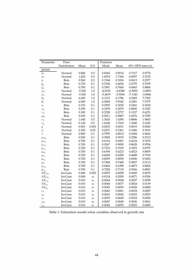
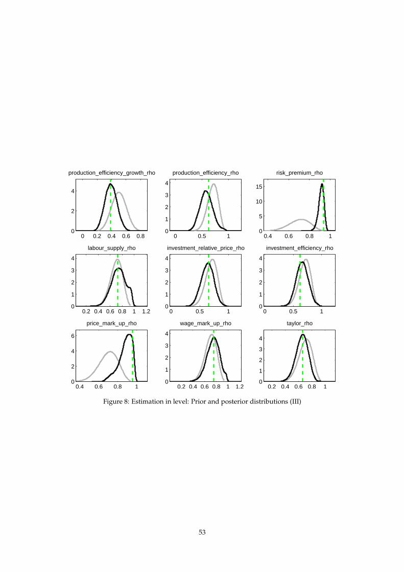
4.3 Estimation results
Following on the arguments developed in the first section of the treatment of trends in DSGE
models, we perform two estimation. The first one uses the rate of growth of GDP, private con-
sumption, private investment and CPI inflation. In the second, we use instead the logarithm
of the level of these variables. The resuls are given in Tables 1 and 2. The prior and posterior
distribution of the parameters are represented in Figures 1 to 10.
Comparing the estimation results, one observes that estimating in the growth rate or in the level
of the variables doesn’t affect greatly the estimation results. For several parameters, the posterior
distribution is very close to the prior. This indicates that the parameters are not identified (or
that the prior is too tight). This is in part the consequence of a relatively short estimation sample.
One could consider using additional observable variables, notably for the behavior of the labor
market, but it could also lead to the reformulation of a more parsimonious model.
It appears that the data suggest an estimated value for the probability of not receiving a positive
signal for a price change, ξp, is 0.37, noticeably lower than the prior mean of 0.72, and than the
usual findings for Europe or the U.S. If confirmed, this result could suggest smaller nominal
rigidities on the good markets in Japan.
The estimation of the monetary policy rule suggests that the inertia of the policy rule as measured
by ρR is less important than expected. On the other hand, the reaction to the output gap, ry , is
more important. Given the fact that the zero lower bound for nominal interest rate is binding over
a large part of the sample, one should be careful not to infer too much from these results about
41

the behavior of the central bank.
Finally, writing the model with the log of interest rate instead of interest rate itself—in order
to insure that the nominal interest rate remains non–negative—doesn’t affect the estimation re-
sults, even for the parameters of the monetary policy rule. In fact, it appears that if log–linear
approximation of nominal interest rate is able to mechanically constrain the model to generate
non–negative levels of the nominal interest rate, it fails to diffuse the consequence of the zero
lower bound to the other parts of the model.
5 Conclusion
In this paper, we discuss the issue of integrating trends in DSGE models. We show how it is
possible to estimate trends and cycle components simultaneously, without detrending the data.
In order to illustrate this methodology, we estimate a DSGE model with standard features on
Japanese data. We explore two different approaches. One estimates the model on the growth
rate of nonstationary variables, the other estimates with the original variables in level. In the
latter case, we need to use the diffuse Kalman filter. Examination of the estimation results shows
very little differences between both approaches. If this equivalence results is confirmed in other
studies, it would mean that there is not much gain to use the most complicated procedure with
the diffuse Kalman filter.
In this paper, we also study the possibility to compute a linear approximation of the logarithm
of nominal interest rate in order to satisfy the zero lower bound. However, this procedure fails
to transmit the effects of the zero lower bound to the rest of the model. This result confirms that
there is no simple escape to the necessity of using nonlinear methods to handle the zero lower
bound and these methods are not available for models of the size considered in this paper.
As often, the results in this paper are preliminary and should be completed by further study. An
interesting development would be to estimate the same model on a longer dataset.
42

References
A. Dixit and J. Stiglitz. Monopolistic Competition and Optimum Product Diversity. American
Economic Review, 67(3):297–308, 1977.
Michael Dotsey and Robert G. King. Implications of state-dependent pricing for dynamic macroe-
conomic models. Working Papers 05-2, Federal Reserve Bank of Philadelphia, February 2005.
Miles S. Kimball. The quantitative analytics of the basic neomonetarist model. NBER Working
Papers 5046, National Bureau of Economic Research, March 1996.
Andrew T. Levin, J. David Lopez-Salido, and Tack Yun. Strategic complementarities and optimal
monetary policy. Kiel Working Papers 1355, Kiel Institute for the World Economy, June 2007.
Frank Smets and Rafael Wouters. Shocks and frictions in us business cycles: A bayesian dsge
approach. American Economic Review, 97(3):586–606, June 2007.
T.Sugo and K. Ueda. Estimating a dsge model for japan: Evaluating and modifying a
cee/sw/loww model. Working Paper 07-E-2, Bank of Japan, 2007.
43
Parameter Prior PosteriorDistribution Mean S.D. Mode Mean 90% HPD interval
paramσc Normal 0.840 0.5 0.8360 0.8514 0.7317 0.9776σl Normal 1.820 0.5 1.8374 1.7180 0.8957 2.5315η Beta 0.560 0.2 0.1544 0.1836 0.0615 0.2977ξp Beta 0.720 0.1 0.3700 0.4056 0.2759 0.5355ξw Beta 0.790 0.1 0.7891 0.7840 0.6965 0.8806ψf Normal -5.500 1.0 -4.8195 -4.8380 -6.5855 -3.0893ψs Normal -5.500 1.0 -5.4679 -5.5056 -7.1343 -3.8966θf Normal 6.000 1.0 6.1215 6.1786 4.5482 7.7292θs Normal 6.000 1.0 6.0068 5.9342 4.2381 7.5375α Beta 0.333 0.1 0.2955 0.3030 0.2441 0.3650γp Beta 0.290 0.1 0.1878 0.2079 0.0830 0.3347γw Beta 0.300 0.1 0.2528 0.2757 0.1237 0.4251ρR Beta 0.830 0.1 0.5811 0.5807 0.4576 0.7055rπ Normal 1.640 0.5 1.3620 1.4290 0.8806 1.9603ry Normal 0.140 0.5 1.6246 1.7418 1.2600 2.2245g Normal 0.003 0.001 0.0033 0.0031 0.0019 0.0043ψ Normal 0.200 0.05 0.2251 0.2361 0.1686 0.3031z Normal 0.800 0.1 0.7995 0.8012 0.6384 0.9662ρAT Beta 0.500 0.1 0.3828 0.3919 0.2586 0.5313ρAC Beta 0.700 0.1 0.6114 0.6001 0.4234 0.7670ρεB Beta 0.700 0.1 0.9267 0.9090 0.8628 0.9556ρεL Beta 0.700 0.1 0.7232 0.7035 0.5453 0.8797ρpI Beta 0.700 0.1 0.6394 0.6223 0.4523 0.8005ρεI Beta 0.700 0.1 0.6069 0.6289 0.4688 0.7918ρεy Beta 0.700 0.1 0.8295 0.8050 0.6906 0.9283ρεl Beta 0.700 0.1 0.7468 0.7400 0.5857 0.9113ρεR Beta 0.700 0.1 0.6464 0.6388 0.4873 0.8002ρεg Beta 0.700 0.1 0.7284 0.7135 0.5566 0.8891SEAT InvGam 0.008 0.002 0.0055 0.0058 0.0045 0.0070SEAC InvGam 0.008 ∞ 0.0154 0.0209 0.0071 0.0356SEεB InvGam 0.010 ∞ 0.0044 0.0048 0.0037 0.0058SEεL InvGam 0.010 ∞ 0.0046 0.0077 0.0024 0.0139SEpI InvGam 0.010 ∞ 0.0045 0.0055 0.0028 0.0080εI InvGam 0.010 ∞ 0.0062 0.0061 0.0034 0.0087εy InvGam 0.010 ∞ 0.0043 0.0042 0.0032 0.0053εl InvGam 0.010 ∞ 0.0035 0.0040 0.0024 0.0056εR InvGam 0.010 ∞ 0.0047 0.0049 0.0036 0.0061εg InvGam 0.010 ∞ 0.0042 0.0055 0.0025 0.0085
Table 1: Estimation results when variables observed in growth rate
44

Parameter Prior PosteriorDistribution Mean S.D. Mode Mean 90% HPD interval
paramσc Normal 0.840 0.5 0.8416 0.8733 0.7490 0.9941σl Normal 1.820 0.5 1.8109 1.7364 0.9046 2.5482η Beta 0.560 0.2 0.1470 0.1703 0.0559 0.2828ξp Beta 0.720 0.1 0.3723 0.4238 0.2802 0.5639ξw Beta 0.790 0.1 0.7912 0.7937 0.7073 0.8852ψf Normal -5.500 1.0 -4.8310 -4.9054 -6.7187 -3.1115ψs Normal -5.500 1.0 -5.4719 -5.4792 -7.1547 -3.8521θf Normal 6.000 1.0 6.0785 6.1190 4.5867 7.6886θs Normal 6.000 1.0 6.0015 5.9678 4.3716 7.6729α Beta 0.333 0.1 0.2909 0.3008 0.2396 0.3635γp Beta 0.290 0.1 0.1869 0.2072 0.0762 0.3326γw Beta 0.300 0.1 0.2533 0.2738 0.1170 0.4187ρR Beta 0.830 0.1 0.5884 0.5848 0.4609 0.7074rπ Normal 1.640 0.5 1.3831 1.4258 0.8678 1.9658ry Normal 0.140 0.5 1.6456 1.7311 1.2517 2.2057g Normal 0.003 0.001 0.0032 0.0031 0.0019 0.0042ψ Normal 0.200 0.05 0.2263 0.2375 0.1667 0.3055z Normal 0.800 0.1 0.8002 0.7999 0.6377 0.9666ρAT Beta 0.500 0.1 0.3821 0.3906 0.2566 0.5257ρAC Beta 0.700 0.1 0.6152 0.5819 0.4041 0.7563ρεB Beta 0.700 0.1 0.9315 0.9155 0.8741 0.9572ρεL Beta 0.700 0.1 0.7232 0.7153 0.5518 0.8824ρpI Beta 0.700 0.1 0.6452 0.6277 0.4603 0.7998ρεI Beta 0.700 0.1 0.6084 0.6331 0.4633 0.7970ρεy Beta 0.700 0.1 0.8497 0.8233 0.7142 0.9329ρεl Beta 0.700 0.1 0.7491 0.7469 0.5925 0.9135ρεR Beta 0.700 0.1 0.6483 0.6492 0.4989 0.7992ρεg Beta 0.700 0.1 0.7287 0.7188 0.5574 0.8878SEAT InvGam 0.008 0.002 0.0054 0.0057 0.0045 0.0070SEAC InvGam 0.008 ∞ 0.0153 0.0242 0.0068 0.0436SEεB InvGam 0.010 ∞ 0.0043 0.0047 0.0037 0.0057SEεL InvGam 0.010 ∞ 0.0046 0.0129 0.0021 0.0274SEpI InvGam 0.010 ∞ 0.0044 0.0056 0.0029 0.0082εI InvGam 0.010 ∞ 0.0063 0.0062 0.0034 0.0088εy InvGam 0.010 ∞ 0.0044 0.0043 0.0032 0.0053εl InvGam 0.010 ∞ 0.0034 0.0041 0.0024 0.0057εR InvGam 0.010 ∞ 0.0047 0.0048 0.0036 0.0061εg InvGam 0.010 ∞ 0.0042 0.0056 0.0025 0.0088
Table 2: Estimation results when variables observed in level
45

Parameter Prior PosteriorDistribution Mean S.D. Mode Mean 90% HPD interval
paramσc Normal 0.840 0.5 0.8363 0.8666 0.7484 0.9841σl Normal 1.820 0.5 1.8375 1.6822 0.8894 2.5228η Beta 0.560 0.2 0.1543 0.1816 0.0633 0.3008ξp Beta 0.720 0.1 0.3700 0.4159 0.2712 0.5629ξw Beta 0.790 0.1 0.7890 0.7883 0.6947 0.8752ψf Normal -5.500 1.0 -4.8115 -4.8997 -6.6244 -3.1827ψs Normal -5.500 1.0 -5.4605 -5.5124 -7.1231 -3.8352θf Normal 6.000 1.0 6.1878 6.1482 4.6174 7.7365θs Normal 6.000 1.0 6.0094 5.9689 4.3131 7.6758α Beta 0.333 0.1 0.2952 0.3057 0.2453 0.3672γp Beta 0.290 0.1 0.1882 0.2080 0.0793 0.3357γw Beta 0.300 0.1 0.2531 0.2727 0.1200 0.4172ρR Beta 0.830 0.1 0.5819 0.5836 0.4506 0.7044rπ Normal 1.640 0.5 1.3667 1.4289 0.8599 1.9573ry Normal 0.140 0.5 1.6321 1.7370 1.2569 2.2119g Normal 0.003 0.001 0.0033 0.0031 0.0019 0.0042ψ Normal 0.200 0.05 0.2249 0.2357 0.1667 0.3021z Normal 0.800 0.1 0.8000 0.8011 0.6386 0.9618ρAT Beta 0.500 0.1 0.3824 0.3925 0.2594 0.5273ρAC Beta 0.700 0.1 0.6115 0.5884 0.4122 0.7677ρεB Beta 0.700 0.1 0.9267 0.9110 0.8660 0.9549ρεL Beta 0.700 0.1 0.7232 0.7051 0.5433 0.8786ρpI Beta 0.700 0.1 0.6396 0.6228 0.4554 0.7973ρεI Beta 0.700 0.1 0.6075 0.6292 0.4673 0.7934ρεy Beta 0.700 0.1 0.8293 0.7993 0.6844 0.9286ρεl Beta 0.700 0.1 0.7478 0.7420 0.5832 0.9042ρεR Beta 0.700 0.1 0.6472 0.6400 0.4849 0.7960ρεg Beta 0.700 0.1 0.7285 0.7175 0.5523 0.8736SEAT InvGam 0.008 0.002 0.0055 0.0057 0.0045 0.0070SEAC InvGam 0.008 ∞ 0.0154 0.0234 0.0066 0.0429SEεB InvGam 0.010 ∞ 0.0044 0.0048 0.0038 0.0057SEεL InvGam 0.010 ∞ 0.0046 0.0138 0.0023 0.0387SEpI InvGam 0.010 ∞ 0.0045 0.0056 0.0029 0.0081εI InvGam 0.010 ∞ 0.0062 0.0061 0.0034 0.0088εy InvGam 0.010 ∞ 0.0043 0.0042 0.0031 0.0053εl InvGam 0.010 ∞ 0.0035 0.0041 0.0024 0.0058εR InvGam 0.010 ∞ 0.0047 0.0048 0.0036 0.0060εg InvGam 0.010 ∞ 0.0042 0.0054 0.0025 0.0083
Table 3: Estimation results for approximation around the log of interest rate
46

0 1 20
2
4
6sigmac
−2 0 2 40
0.2
0.4
0.6
0.8
sigmal
0 0.2 0.4 0.6 0.80
2
4
eta
0 0.2 0.4 0.6 0.80
1
2
3
4
xip
0.2 0.4 0.6 0.8 10
2
4
6
xiw
−10 −5 00
0.1
0.2
0.3
0.4
psif
−10 −5 00
0.1
0.2
0.3
0.4
psis
2 4 6 8 10 120
0.1
0.2
0.3
0.4
thetaf
0 5 100
0.1
0.2
0.3
0.4
thetas
Figure 1: Estimation in growth rate: Prior and posterior distributions (I)
47

0.2 0.4 0.60
5
10
alpha
0 0.2 0.4 0.6 0.80
2
4
gammap
−0.2 0 0.2 0.4 0.6 0.80
1
2
3
4
gammaw
0.2 0.4 0.6 0.8 10
2
4
nominal_interest_rate_smoothing
0 1 2 30
0.5
1
elasticity_of_nominal_interest_rate_to_inflation
−1 0 1 2 30
0.5
1
elasticity_of_nominal_interest_rate_to_output_gap
−2 0 2 4 6 8
x 10−3
0
100
200
300
400
production_efficiency_growth_ss
0 0.2 0.40
5
10investment_cost_size
0.2 0.4 0.6 0.8 1 1.2 1.40
1
2
3
4
capacity_utilization_factor_ss
Figure 2: Estimation in growth rate: Prior and posterior distributions (II)
48

0 0.2 0.4 0.6 0.80
2
4
production_efficiency_growth_rho
0 0.5 10
1
2
3
4
production_efficiency_rho
0.4 0.6 0.8 10
5
10
risk_premium_rho
0.2 0.4 0.6 0.8 1 1.20
1
2
3
4
labour_supply_rho
0 0.5 10
1
2
3
4
investment_relative_price_rho
0.2 0.4 0.6 0.8 1 1.20
1
2
3
4
investment_efficiency_rho
0.4 0.6 0.8 10
2
4
price_mark_up_rho
0.2 0.4 0.6 0.8 10
1
2
3
4
wage_mark_up_rho
0.2 0.4 0.6 0.8 10
1
2
3
4
taylor_rho
Figure 3: Estimation in growth rate: Prior and posterior distributions (III)
49

0.2 0.4 0.6 0.8 10
1
2
3
4
public_spending_rho
2 4 6 8 10 12 14
x 10−3
0
200
400
production_efficiency_growth_i_std
0 0.05 0.10
50
100
150
production_efficiency_i_std
0.01 0.02 0.03 0.04 0.050
200
400
600
risk_premium_i_std
0 0.02 0.04 0.060
50
100
150
labour_supply_i_std
0 0.02 0.040
50
100
150
200
investment_relative_price_i_std
0 0.02 0.040
100
200
investment_efficiency_i_std
0 0.02 0.040
200
400
600
price_mark_up_i_std
0 0.02 0.040
100
200
300
400
wage_mark_up_i_std
Figure 4: Estimation in growth rate: Prior and posterior distributions (IV)
0 0.02 0.040
200
400
taylor_i_std
0 0.02 0.040
100
200
public_spending_i_std
Figure 5: Estimation in growth rate: Prior and posterior distributions (V)
50

0 1 20
2
4
6
sigmac
0 2 40
0.2
0.4
0.6
0.8
sigmal
0 0.2 0.4 0.6 0.80
2
4
eta
0 0.2 0.4 0.6 0.80
1
2
3
4
xip
0.2 0.4 0.6 0.8 10
2
4
6
xiw
−10 −5 00
0.1
0.2
0.3
0.4
psif
−10 −5 00
0.1
0.2
0.3
0.4
psis
0 5 100
0.1
0.2
0.3
0.4
thetaf
0 5 100
0.1
0.2
0.3
0.4
thetas
Figure 6: Estimation in level: Prior and posterior distributions (I)
51

0.2 0.4 0.60
5
10
alpha
0 0.2 0.4 0.60
2
4
gammap
0 0.2 0.4 0.6 0.80
1
2
3
4
gammaw
0.2 0.4 0.6 0.8 10
2
4
nominal_interest_rate_smoothing
0 1 2 30
0.5
1
elasticity_of_nominal_interest_rate_to_inflation
−1 0 1 2 30
0.5
1
1.5elasticity_of_nominal_interest_rate_to_output_gap
−2 0 2 4 6 8
x 10−3
0
200
400
production_efficiency_growth_ss
0 0.2 0.40
5
10investment_cost_size
0.2 0.4 0.6 0.8 1 1.2 1.40
1
2
3
4
capacity_utilization_factor_ss
Figure 7: Estimation in level: Prior and posterior distributions (II)
52
0 0.2 0.4 0.6 0.80
2
4
production_efficiency_growth_rho
0 0.5 10
1
2
3
4
production_efficiency_rho
0.4 0.6 0.8 10
5
10
15
risk_premium_rho
0.2 0.4 0.6 0.8 1 1.20
1
2
3
4
labour_supply_rho
0 0.5 10
1
2
3
4
investment_relative_price_rho
0 0.5 10
1
2
3
4
investment_efficiency_rho
0.4 0.6 0.8 10
2
4
6
price_mark_up_rho
0.2 0.4 0.6 0.8 1 1.20
1
2
3
4
wage_mark_up_rho
0.2 0.4 0.6 0.8 10
1
2
3
4
taylor_rho
Figure 8: Estimation in level: Prior and posterior distributions (III)
53

0 0.5 10
1
2
3
4
public_spending_rho
2 4 6 8 10 12 14
x 10−3
0
200
400
production_efficiency_growth_i_std
−0.02 0 0.020.040.060.080
50
100
150
production_efficiency_i_std
0.01 0.02 0.03 0.04 0.050
200
400
600
risk_premium_i_std
0 0.05 0.10
50
100
150
labour_supply_i_std
0 0.02 0.040
50
100
150
200
investment_relative_price_i_std
0 0.02 0.040
50
100
150
200
investment_efficiency_i_std
0 0.02 0.040
200
400
600
price_mark_up_i_std
0 0.02 0.040
100
200
300
400
wage_mark_up_i_std
Figure 9: Estimation in level: Prior and posterior distributions (IV)
0.01 0.02 0.03 0.04 0.050
200
400
600taylor_i_std
0 0.02 0.040
50
100
150
200
public_spending_i_std
Figure 10: Estimation in level: Prior and posterior distributions (V)
54


