Data Mining – Intro
Course Overview
Spatial Databases Temporal Databases Spatio-Temporal Databases Data Mining
Data Mining Overview
Data Mining Data warehouses and OLAP (On Line Analytical
Processing.) Association Rules Mining Clustering: Hierarchical and Partitional
approaches Classification: Decision Trees and Bayesian
classifiers Sequential Patterns Mining Advanced topics: outlier detection, web mining
What is Data Mining?
Data Mining is:(1) The efficient discovery of previously
unknown, valid, potentially useful, understandable patterns in large datasets
(2) The analysis of (often large) observational data sets to find unsuspected relationships and to summarize the data in novel ways that are both understandable and useful to the data owner

What is Data Mining?
Very little functionality in database systems to support mining applications
Beyond SQL Querying: SQL (OLAP) Query:
- How many widgets did we sell in the 1st Qtr of 1999 in California vs New York?
Data Mining Queries:- Which sales region had anomalous sales in the 1st Qtr of 1999
- How do the buyers of widgets in California and New York differ?
- What else do the buyers of widgets in Cal buy along with widgets
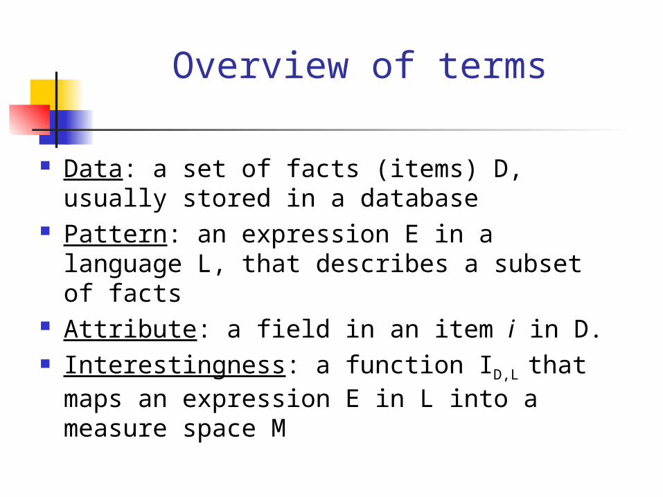
Overview of terms
Data: a set of facts (items) D, usually stored in a database
Pattern: an expression E in a language L, that describes a subset of facts
Attribute: a field in an item i in D. Interestingness: a function ID,L that maps
an expression E in L into a measure space M
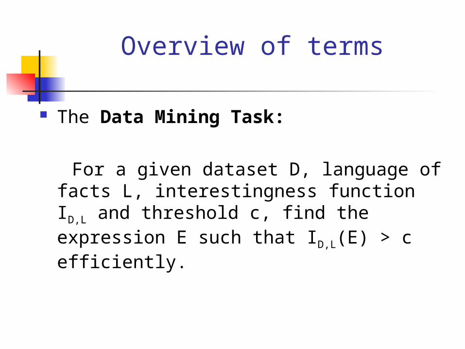
Overview of terms
The Data Mining Task:
For a given dataset D, language of facts L, interestingness function ID,L and threshold c, find the expression E such that ID,L(E) > c efficiently.
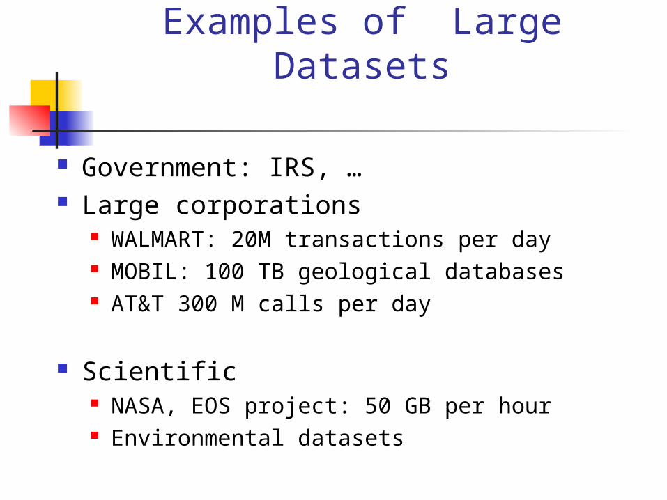
Examples of Large Datasets
Government: IRS, … Large corporations
WALMART: 20M transactions per day MOBIL: 100 TB geological databases AT&T 300 M calls per day
Scientific NASA, EOS project: 50 GB per hour Environmental datasets
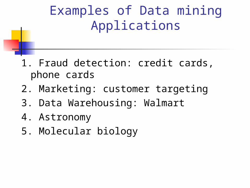
Examples of Data mining Applications
1. Fraud detection: credit cards, phone cards2. Marketing: customer targeting3. Data Warehousing: Walmart4. Astronomy5. Molecular biology
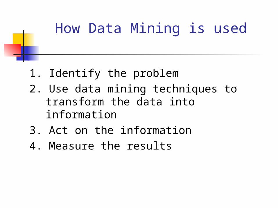
How Data Mining is used
1. Identify the problem2. Use data mining techniques to
transform the data into information3. Act on the information4. Measure the results
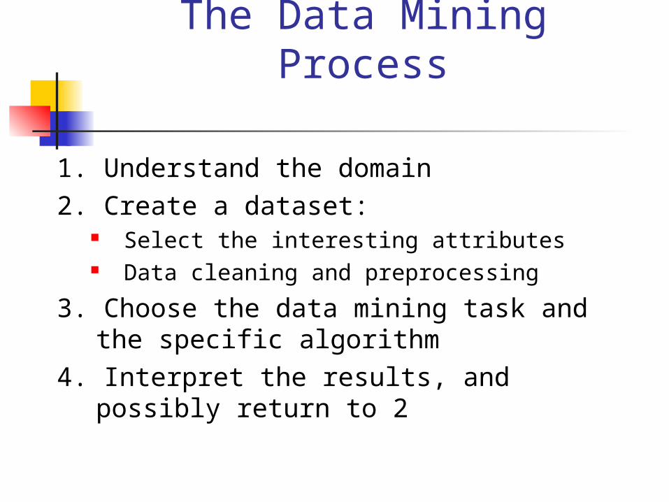
The Data Mining Process
1. Understand the domain2. Create a dataset:
Select the interesting attributes Data cleaning and preprocessing
3. Choose the data mining task and the specific algorithm
4. Interpret the results, and possibly return to 2
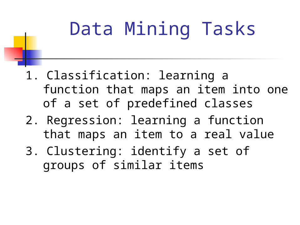
Data Mining Tasks
1. Classification: learning a function that maps an item into one of a set of predefined classes
2. Regression: learning a function that maps an item to a real value
3. Clustering: identify a set of groups of similar items
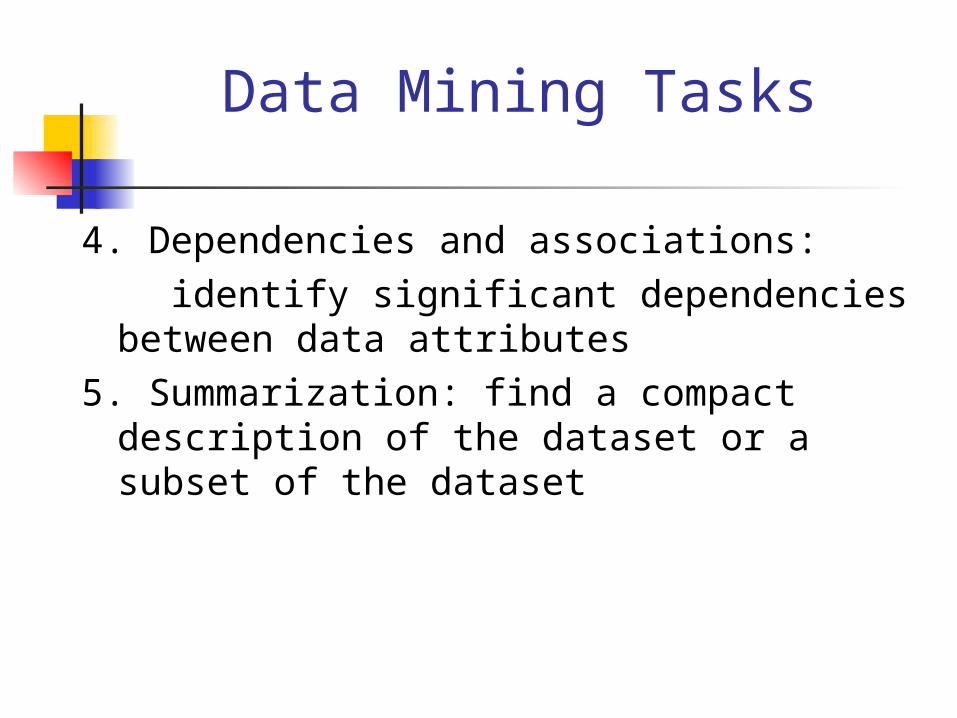
Data Mining Tasks
4. Dependencies and associations: identify significant dependencies between
data attributes5. Summarization: find a compact
description of the dataset or a subset of the dataset
Data Mining Methods
1. Decision Tree Classifiers: Used for modeling, classification
2. Association Rules:Used to find associations between sets of
attributes
3. Sequential patterns:Used to find temporal associations in time series
4. Hierarchical clustering: used to group customers, web users, etc
Are All the “Discovered” Patterns Interesting?
Interestingness measures: A pattern is
interesting if it is easily understood by humans,
valid on new or test data with some degree of
certainty, potentially useful, novel, or validates
some hypothesis that a user seeks to confirm Objective vs. subjective interestingness measures:
Objective: based on statistics and structures of patterns, e.g.,
support, confidence, etc.
Subjective: based on user’s belief in the data, e.g.,
unexpectedness, novelty, actionability, etc.
Can We Find All and Only Interesting Patterns?
Find all the interesting patterns: Completeness Can a data mining system find all the interesting patterns? Association vs. classification vs. clustering
Search for only interesting patterns: Optimization Can a data mining system find only the interesting
patterns? Approaches
First general all the patterns and then filter out the uninteresting ones.
Generate only the interesting patterns—mining query optimization
Why Data Preprocessing?
Data in the real world is dirty incomplete: lacking attribute values, lacking certain
attributes of interest, or containing only aggregate data noisy: containing errors or outliers inconsistent: containing discrepancies in codes or names
No quality data, no quality mining results! Quality decisions must be based on quality data Data warehouse needs consistent integration of quality
data Required for both OLAP and Data Mining!

Why can Data be Incomplete?
Attributes of interest are not available (e.g., customer information for sales transaction data)
Data were not considered important at the time of transactions, so they were not recorded!
Data not recorder because of misunderstanding or malfunctions
Data may have been recorded and later deleted! Missing/unknown values for some data
Why can Data be Noisy/Inconsistent?
Faulty instruments for data collection Human or computer errors Errors in data transmission Technology limitations (e.g., sensor data come at a
faster rate than they can be processed) Inconsistencies in naming conventions or data
codes (e.g., 2/5/2002 could be 2 May 2002 or 5 Feb 2002)
Duplicate tuples, which were received twice should also be removed
Major Tasks in Data Preprocessing
Data cleaning Fill in missing values, smooth noisy data, identify or remove
outliers, and resolve inconsistencies
Data integration Integration of multiple databases or files
Data transformation Normalization and aggregation
Data reduction Obtains reduced representation in volume but produces the
same or similar analytical results
Data discretization Part of data reduction but with particular importance,
especially for numerical data
outliers=exceptions!
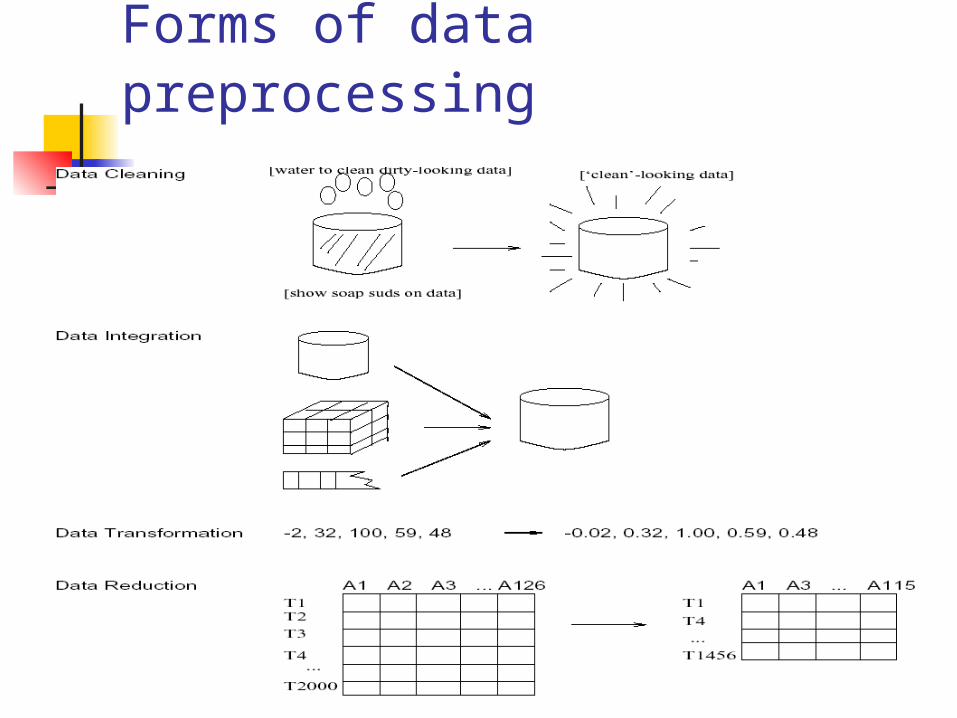
Forms of data preprocessing
Data Cleaning
Data cleaning tasks Fill in missing values
Identify outliers and smooth out noisy data
Correct inconsistent data
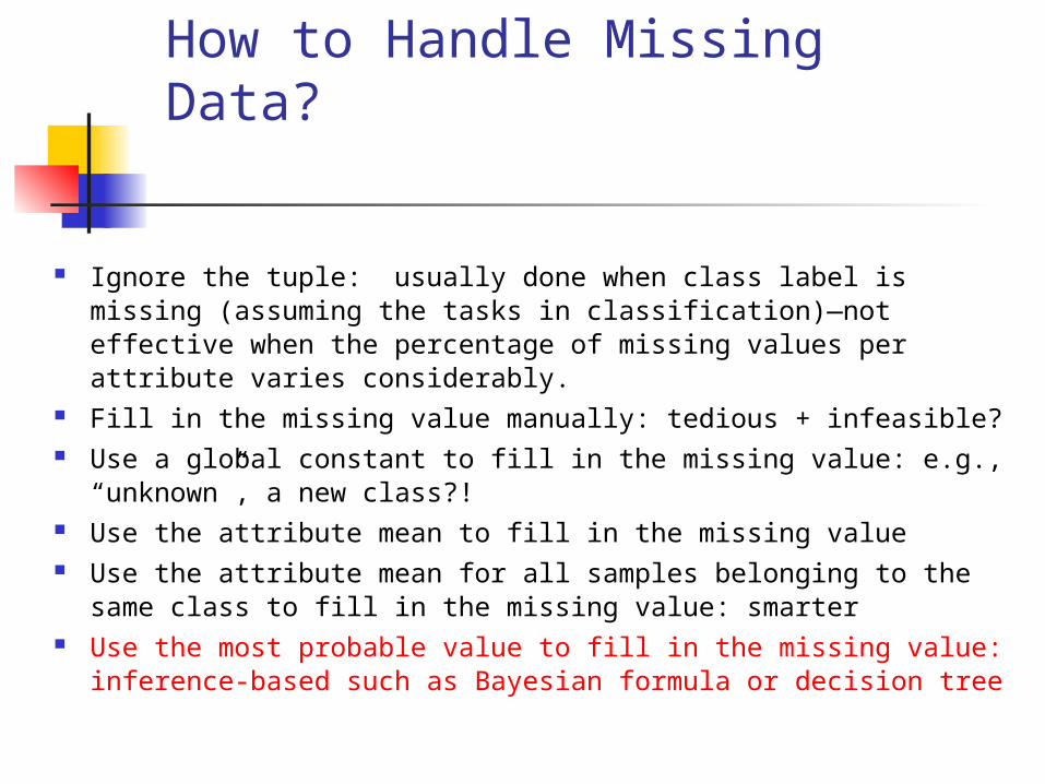
How to Handle Missing Data?
Ignore the tuple: usually done when class label is missing (assuming the tasks in classification)—not effective when the percentage of missing values per attribute varies considerably.
Fill in the missing value manually: tedious + infeasible? Use a global constant to fill in the missing value: e.g.,
“unknown”, a new class?! Use the attribute mean to fill in the missing value Use the attribute mean for all samples belonging to the same
class to fill in the missing value: smarter Use the most probable value to fill in the missing value:
inference-based such as Bayesian formula or decision tree
How to Handle Missing Data?
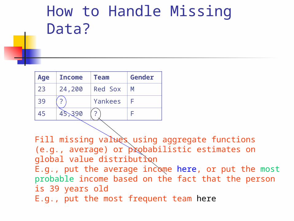
Age Income Team Gender
23 24,200 Red Sox M
39 ? Yankees F
45 45,390 ? F
Fill missing values using aggregate functions (e.g., average) or probabilistic estimates on global value distributionE.g., put the average income here, or put the most probable income based on the fact that the person is 39 years oldE.g., put the most frequent team here
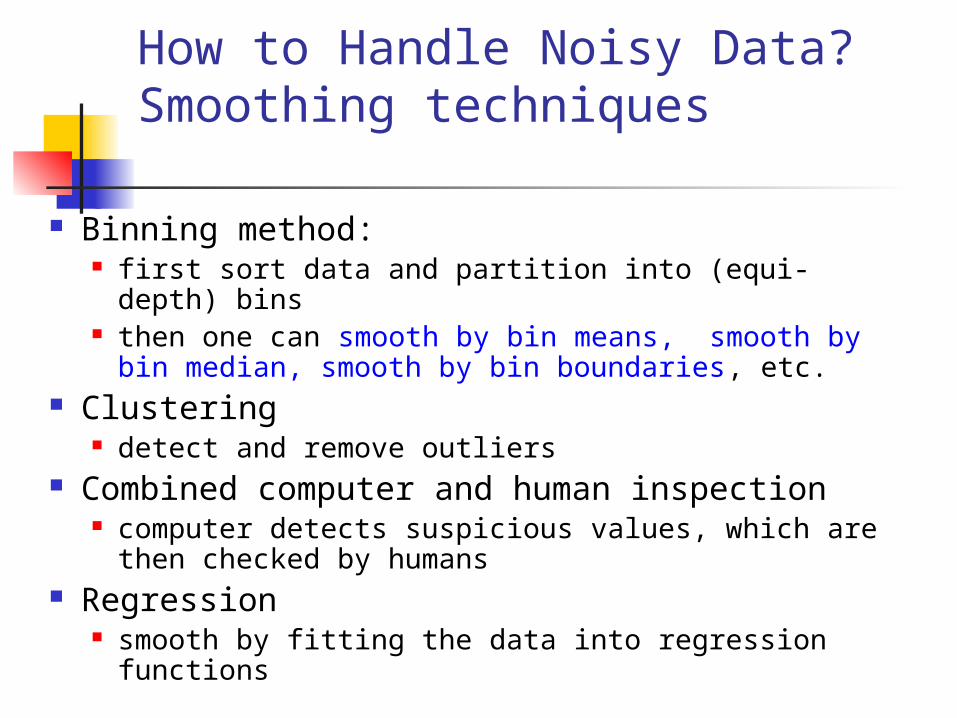
How to Handle Noisy Data?Smoothing techniques
Binning method: first sort data and partition into (equi-depth) bins then one can smooth by bin means, smooth by
bin median, smooth by bin boundaries, etc. Clustering
detect and remove outliers Combined computer and human inspection
computer detects suspicious values, which are then checked by humans
Regression smooth by fitting the data into regression
functions
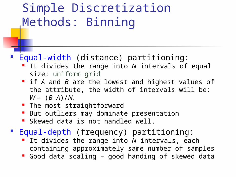
Simple Discretization Methods: Binning
Equal-width (distance) partitioning: It divides the range into N intervals of equal size:
uniform grid if A and B are the lowest and highest values of the
attribute, the width of intervals will be: W = (B-A)/N. The most straightforward But outliers may dominate presentation Skewed data is not handled well.
Equal-depth (frequency) partitioning: It divides the range into N intervals, each containing
approximately same number of samples Good data scaling – good handing of skewed data
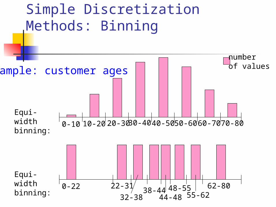
Simple Discretization Methods: Binning
Example: customer ages
0-10 10-20 20-30 30-40 40-50 50-60 60-70 70-80
Equi-width binning:
numberof values
0-22 22-31
44-4832-3838-44 48-55
55-6262-80
Equi-width binning:
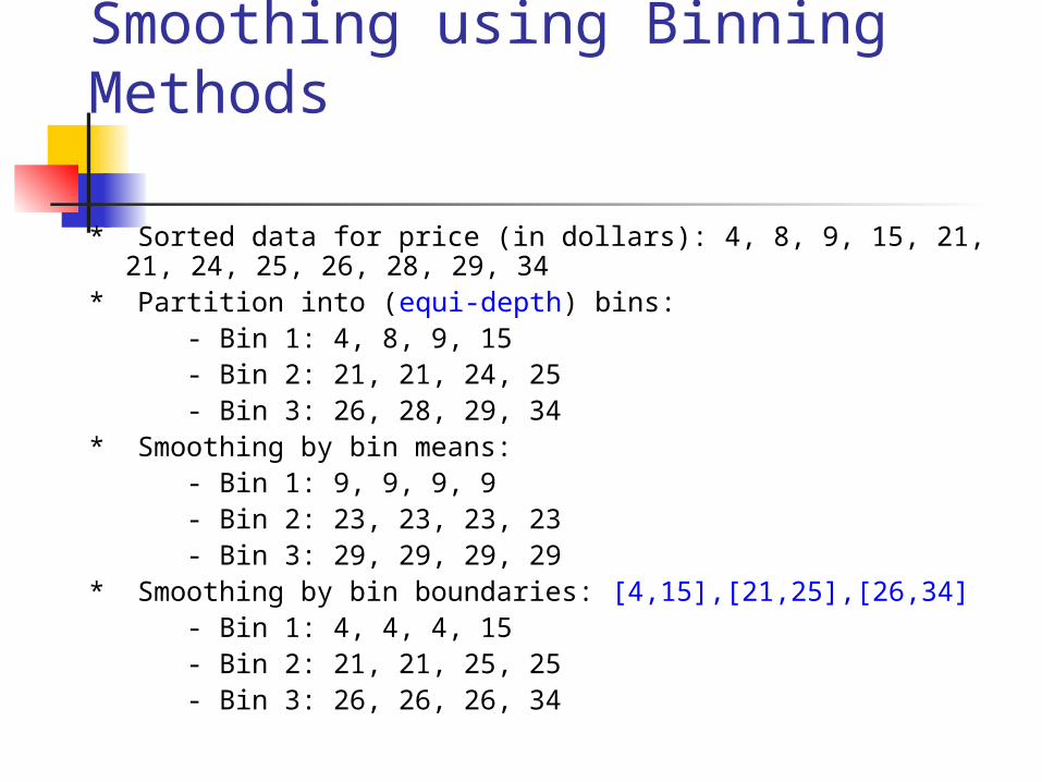
Smoothing using Binning Methods
* Sorted data for price (in dollars): 4, 8, 9, 15, 21, 21, 24, 25, 26, 28, 29, 34
* Partition into (equi-depth) bins: - Bin 1: 4, 8, 9, 15 - Bin 2: 21, 21, 24, 25 - Bin 3: 26, 28, 29, 34* Smoothing by bin means: - Bin 1: 9, 9, 9, 9 - Bin 2: 23, 23, 23, 23 - Bin 3: 29, 29, 29, 29* Smoothing by bin boundaries: [4,15],[21,25],[26,34] - Bin 1: 4, 4, 4, 15 - Bin 2: 21, 21, 25, 25 - Bin 3: 26, 26, 26, 34
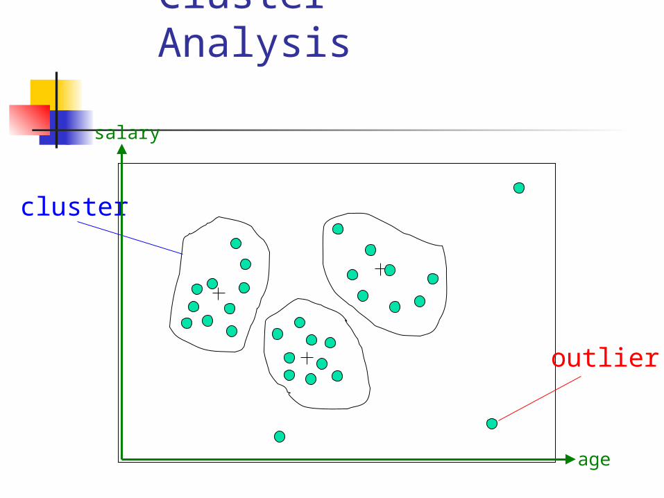
Cluster Analysis
cluster
outlier
salary
age
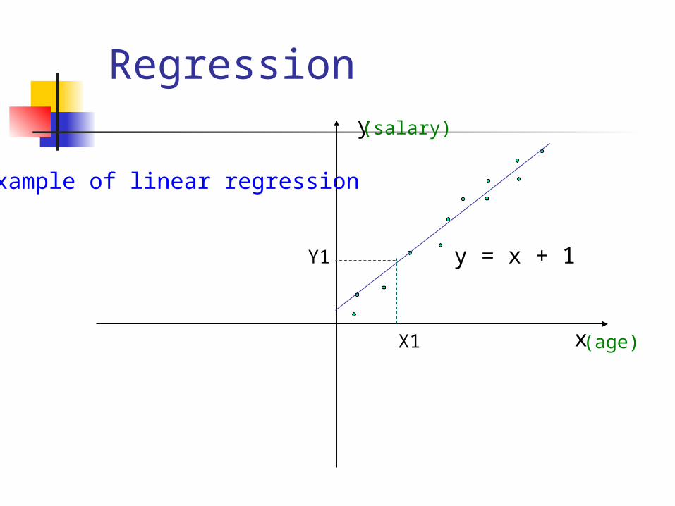
Regression
x
y
y = x + 1
X1
Y1
(salary)
(age)
Example of linear regression
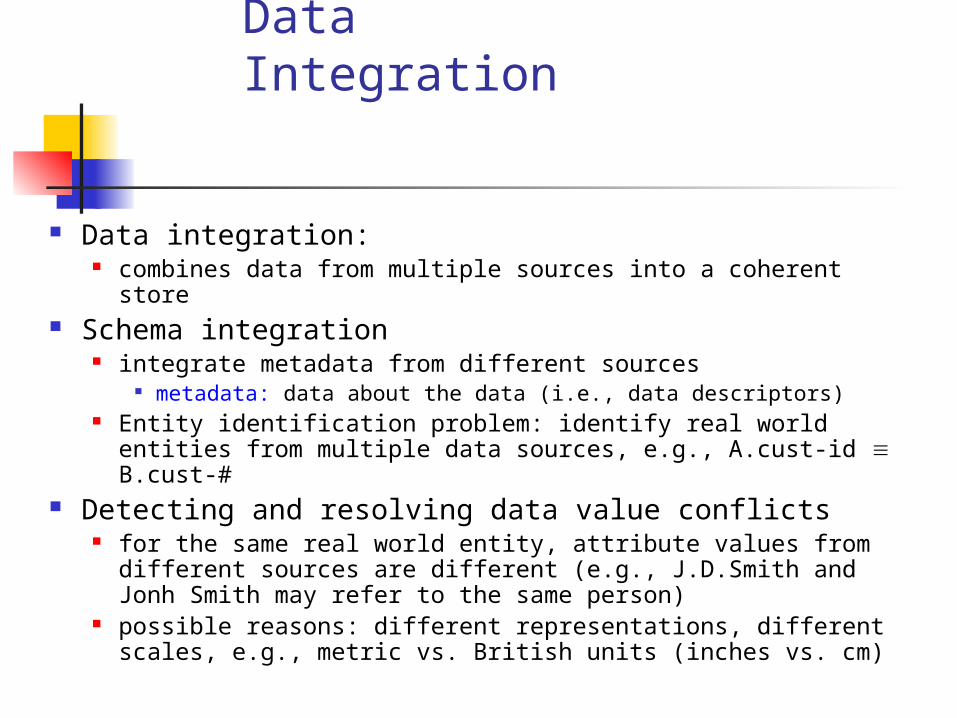
Data Integration
Data integration: combines data from multiple sources into a coherent store
Schema integration integrate metadata from different sources
metadata: data about the data (i.e., data descriptors) Entity identification problem: identify real world entities
from multiple data sources, e.g., A.cust-id B.cust-# Detecting and resolving data value conflicts
for the same real world entity, attribute values from different sources are different (e.g., J.D.Smith and Jonh Smith may refer to the same person)
possible reasons: different representations, different scales, e.g., metric vs. British units (inches vs. cm)
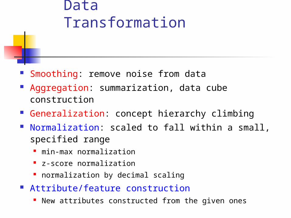
Data Transformation
Smoothing: remove noise from data Aggregation: summarization, data cube
construction Generalization: concept hierarchy climbing Normalization: scaled to fall within a small,
specified range min-max normalization z-score normalization normalization by decimal scaling
Attribute/feature construction New attributes constructed from the given ones

Normalization: Why normalization?
Speeds-up learning, e.g., neural networks Helps prevent attributes with large
ranges outweigh ones with small ranges Example:
income has range 3000-200000 age has range 10-80 gender has domain M/F
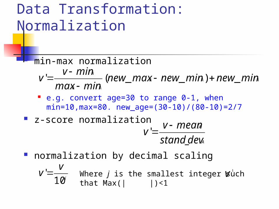
Data Transformation: Normalization
min-max normalization
e.g. convert age=30 to range 0-1, when min=10,max=80. new_age=(30-10)/(80-10)=2/7
z-score normalization
normalization by decimal scaling
AAA
AA
A
minnewminnewmaxnewminmax
minvv _)__('
A
A
devstand_
meanvv
'
j
vv
10' Where j is the smallest integer such that Max(| |)<1'v
Data Reduction Strategies
Warehouse may store terabytes of data: Complex data analysis/mining may take a very long time to run on the complete data set
Data reduction Obtains a reduced representation of the data set
that is much smaller in volume but yet produces the same (or almost the same) analytical results
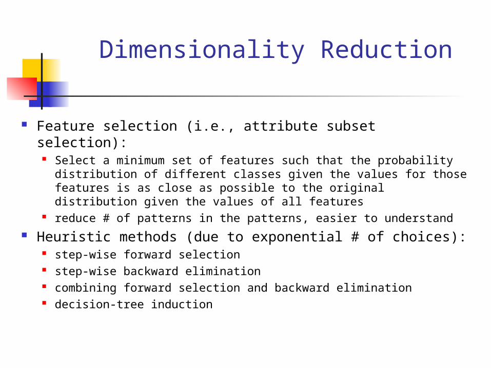
Dimensionality Reduction
Feature selection (i.e., attribute subset selection): Select a minimum set of features such that the probability
distribution of different classes given the values for those features is as close as possible to the original distribution given the values of all features
reduce # of patterns in the patterns, easier to understand Heuristic methods (due to exponential # of choices):
step-wise forward selection step-wise backward elimination combining forward selection and backward elimination decision-tree induction
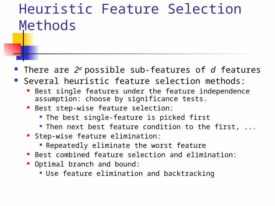
Heuristic Feature Selection Methods
There are 2d possible sub-features of d features Several heuristic feature selection methods:
Best single features under the feature independence assumption: choose by significance tests.
Best step-wise feature selection: The best single-feature is picked first Then next best feature condition to the first, ...
Step-wise feature elimination: Repeatedly eliminate the worst feature
Best combined feature selection and elimination: Optimal branch and bound:
Use feature elimination and backtracking
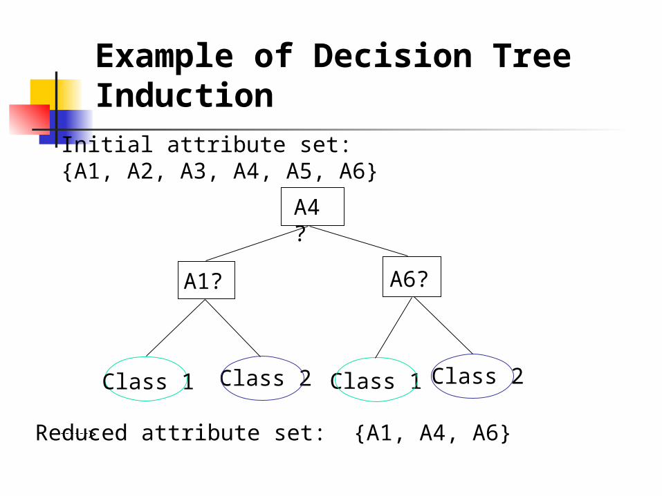
Example of Decision Tree Induction
Initial attribute set:{A1, A2, A3, A4, A5, A6}
A4 ?
A1? A6?
Class 1 Class 2 Class 1 Class 2
> Reduced attribute set: {A1, A4, A6}
Data Compression
String compression There are extensive theories and well-tuned algorithms Typically lossless But only limited manipulation is possible without
expansion Audio/video compression
Typically lossy compression, with progressive refinement Sometimes small fragments of signal can be
reconstructed without reconstructing the whole Time sequence is not audio
Typically short and varies slowly with time

Data Compression
Original Data Compressed Data
lossless
Original DataApproximated
lossy
Numerosity Reduction:Reduce the volume of data
Parametric methods Assume the data fits some model, estimate model
parameters, store only the parameters, and discard the data (except possible outliers)
Log-linear models: obtain value at a point in m-D space as the product on appropriate marginal subspaces
Non-parametric methods Do not assume models Major families: histograms, clustering, sampling
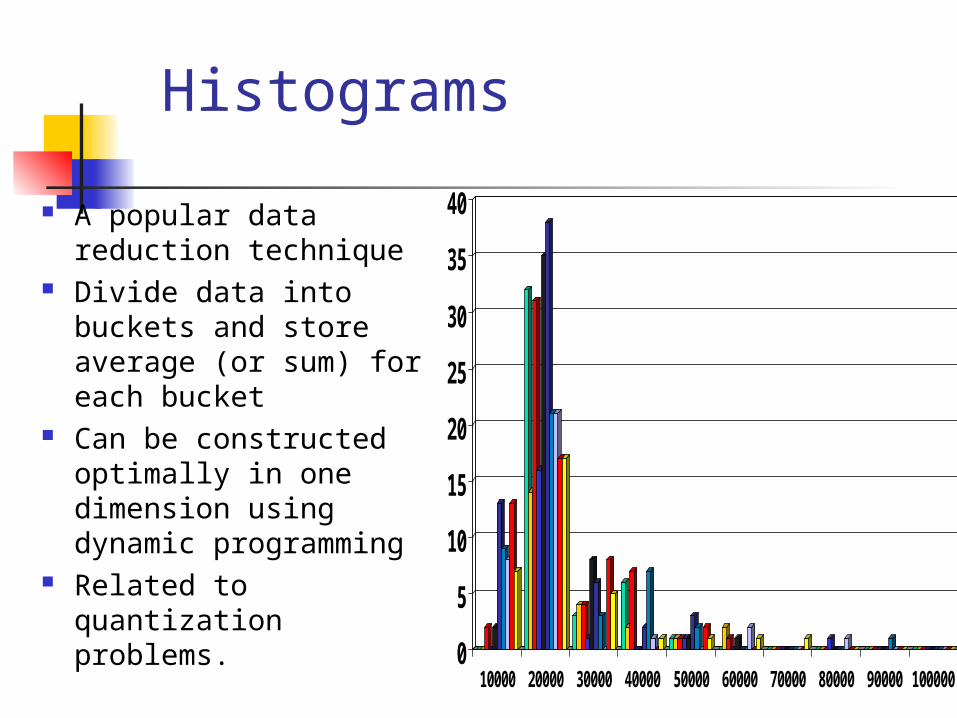
Histograms
A popular data reduction technique
Divide data into buckets and store average (or sum) for each bucket
Can be constructed optimally in one dimension using dynamic programming
Related to quantization problems.
0
5
10
15
20
25
30
35
40
10000 20000 30000 40000 50000 60000 70000 80000 90000 100000
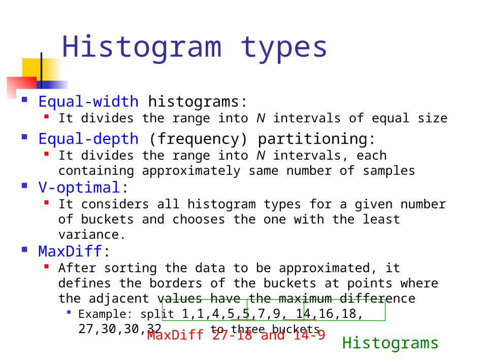
Histogram types
Equal-width histograms: It divides the range into N intervals of equal size
Equal-depth (frequency) partitioning: It divides the range into N intervals, each containing
approximately same number of samples V-optimal:
It considers all histogram types for a given number of buckets and chooses the one with the least variance.
MaxDiff: After sorting the data to be approximated, it defines the
borders of the buckets at points where the adjacent values have the maximum difference
Example: split 1,1,4,5,5,7,9, 14,16,18, 27,30,30,32 to three buckets
MaxDiff 27-18 and 14-9 Histograms
Clustering
Partitions data set into clusters, and models it by
one representative from each cluster
Can be very effective if data is clustered but not
if data is “smeared”
There are many choices of clustering definitions
and clustering algorithms, more later!
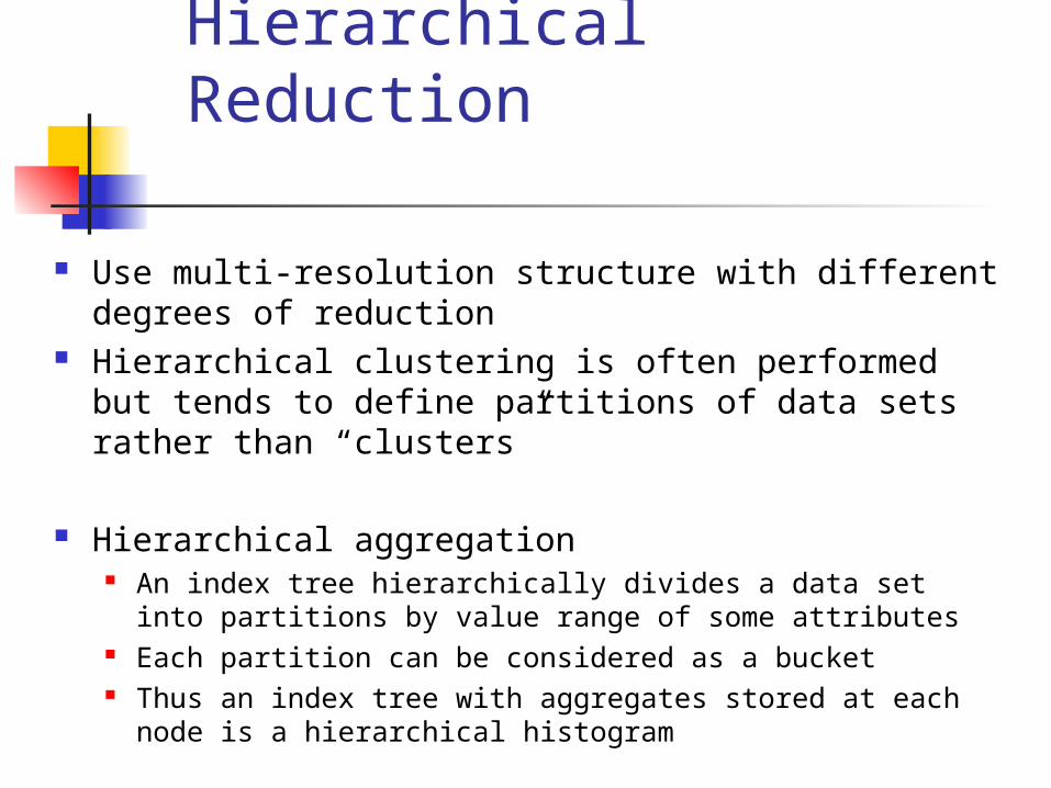
Hierarchical Reduction
Use multi-resolution structure with different degrees of reduction
Hierarchical clustering is often performed but tends to define partitions of data sets rather than “clusters”
Hierarchical aggregation An index tree hierarchically divides a data set into
partitions by value range of some attributes Each partition can be considered as a bucket Thus an index tree with aggregates stored at each node is a
hierarchical histogram
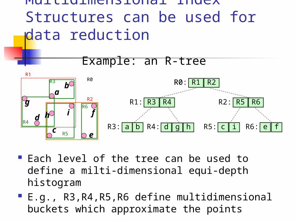
Multidimensional Index Structures can be used for data reduction
R0R1
R2
R3
R4
R5
R6
f
c
g
d h
ba
e
i
R0 (0)
e fc ia b
R5 R6R3 R4
R1 R2
g hd
R0:
R1: R2:
R3: R4: R5: R6:
Example: an R-tree
Each level of the tree can be used to define a milti-dimensional equi-depth histogram
E.g., R3,R4,R5,R6 define multidimensional buckets which approximate the points
Sampling
Allow a mining algorithm to run in complexity that is potentially sub-linear to the size of the data
Choose a representative subset of the data Simple random sampling may have very poor
performance in the presence of skew Develop adaptive sampling methods
Stratified sampling: Approximate the percentage of each class (or
subpopulation of interest) in the overall database Used in conjunction with skewed data
Sampling may not reduce database I/Os (page at a time).
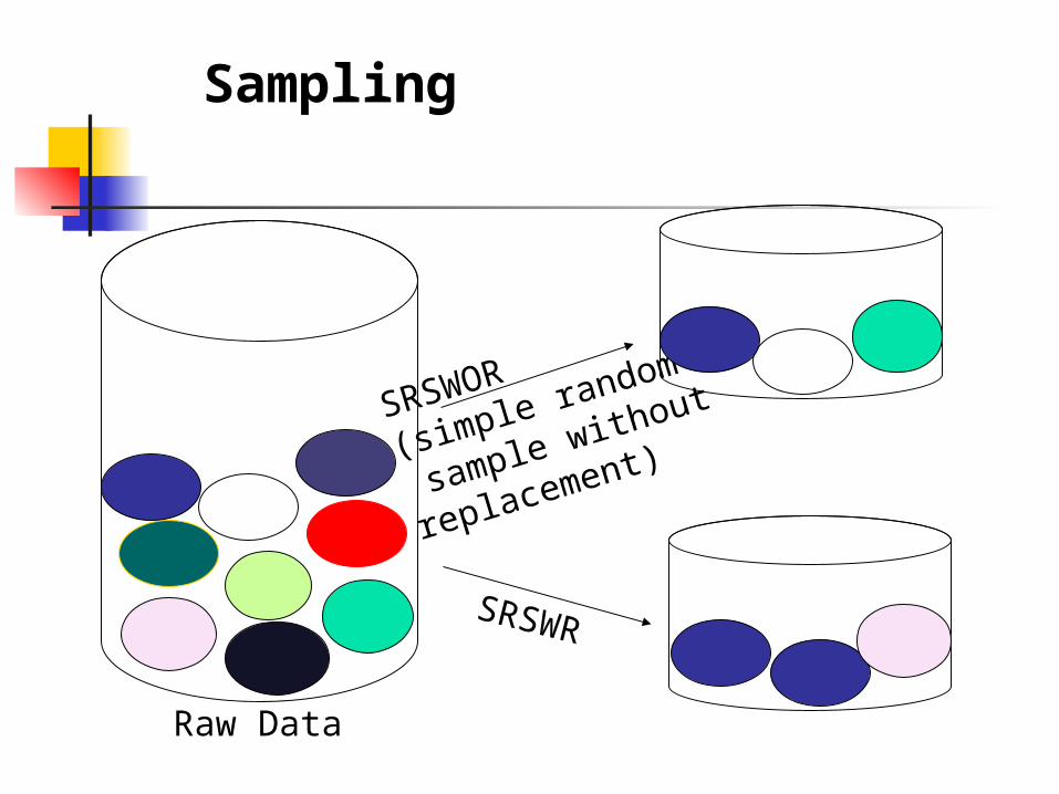
Sampling
SRSWOR
(simple random
sample without
replacement)
SRSWR
Raw Data
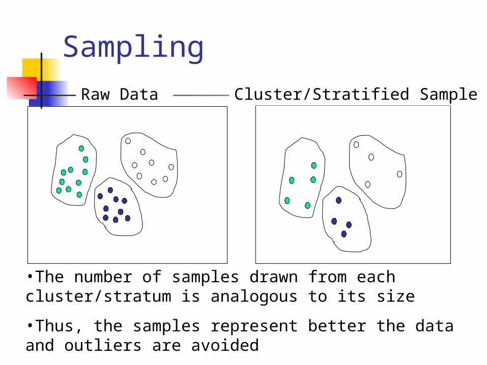
SamplingRaw Data Cluster/Stratified Sample
•The number of samples drawn from each cluster/stratum is analogous to its size
•Thus, the samples represent better the data and outliers are avoided
Summary
Data preparation is a big issue for both warehousing and mining
Data preparation includes Data cleaning and data integration Data reduction and feature selection Discretization
A lot a methods have been developed but still an active area of research


