Download - CS190.1x_week5

Neuroscience Introduction
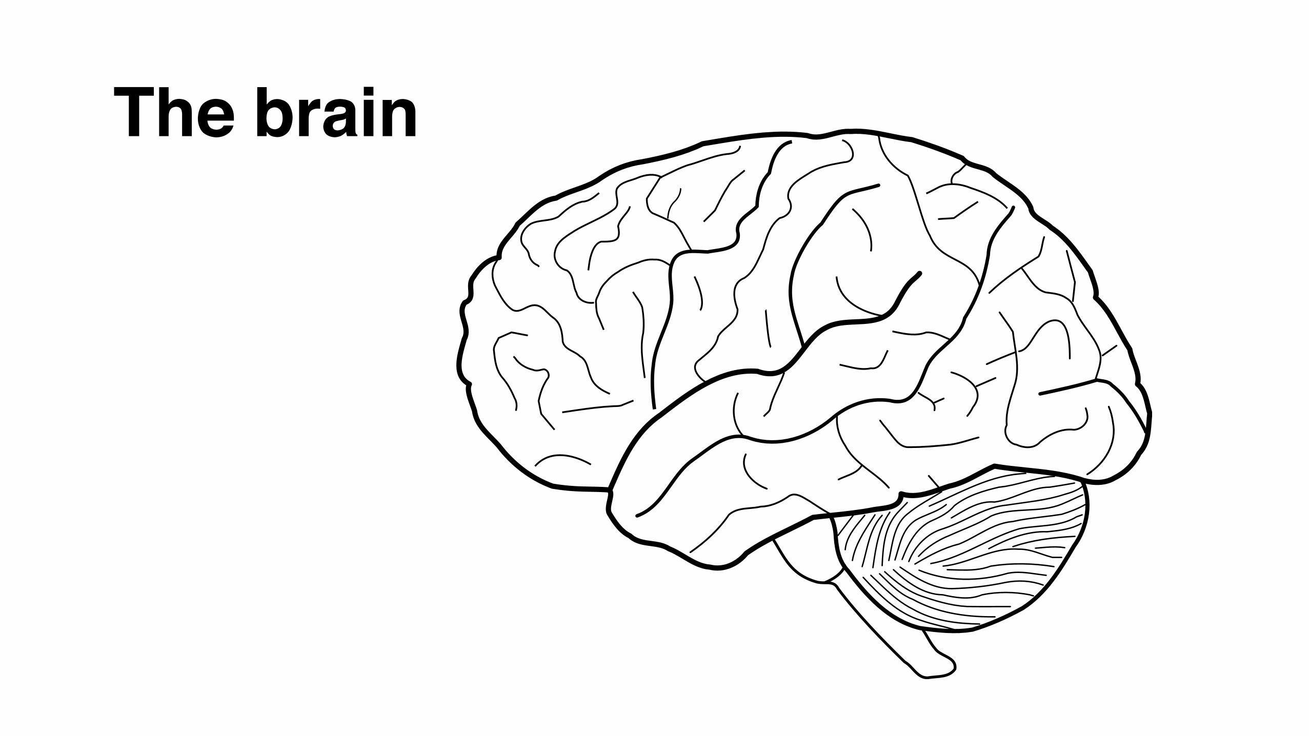
The brain

“As humans, we can identify galaxies light years away, we can study particles smaller than an atom. But we still haven’t unlocked the mystery of the three pounds of matter that sits between our ears.”
President Obama

Stimuli
Behavior
The brain

100 200 300
100 200 300
100 200 300
SnailZebrafish
Ant
FrogMouse
Octopus
ChimpanzeeElephantHuman
Thousands
Millions
Billions
Numbersof neurons

Studying the brain in humans
fMRI scanner human brain


~50,000 neurons per cubic millimeter -> need higher resolution!
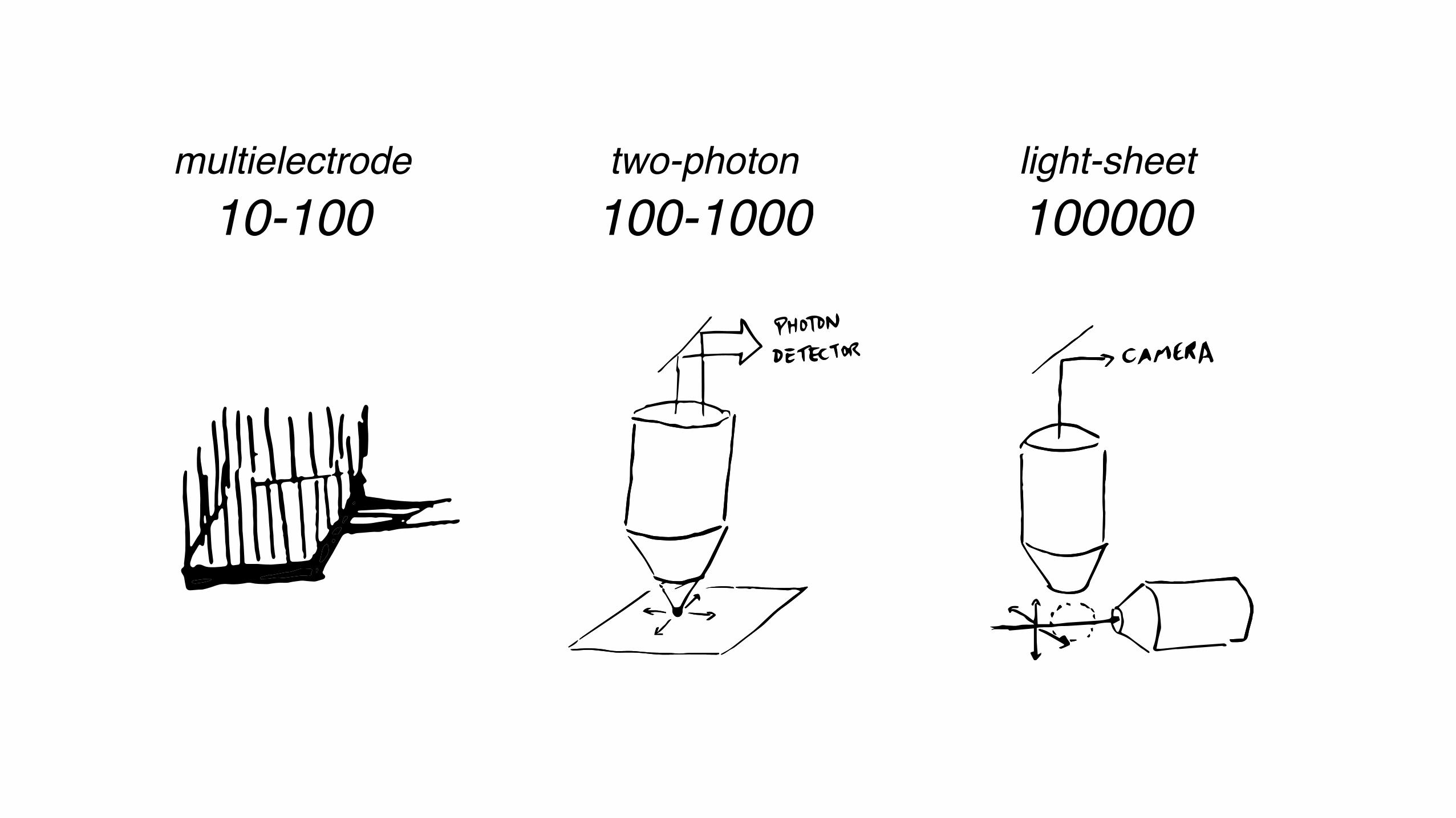
multielectrode10-100
two-photon100-1000
light-sheet100000

Vladimirov, et al., 2014

Sofroniew, et al., 2014

relating neuronal responses to properties of an animal and its environment
Moser et al., 2008
position of a mouse in maze
“place cell” “grid cell”
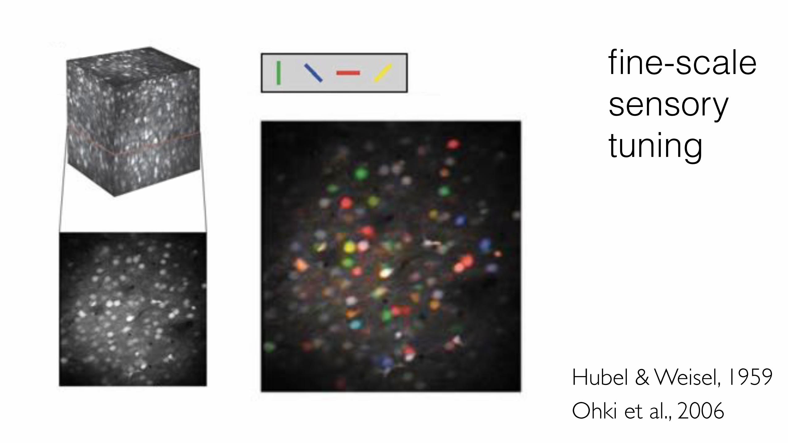
Ohki et al., 2006
fine-scale sensory tuning
Hubel & Weisel, 1959
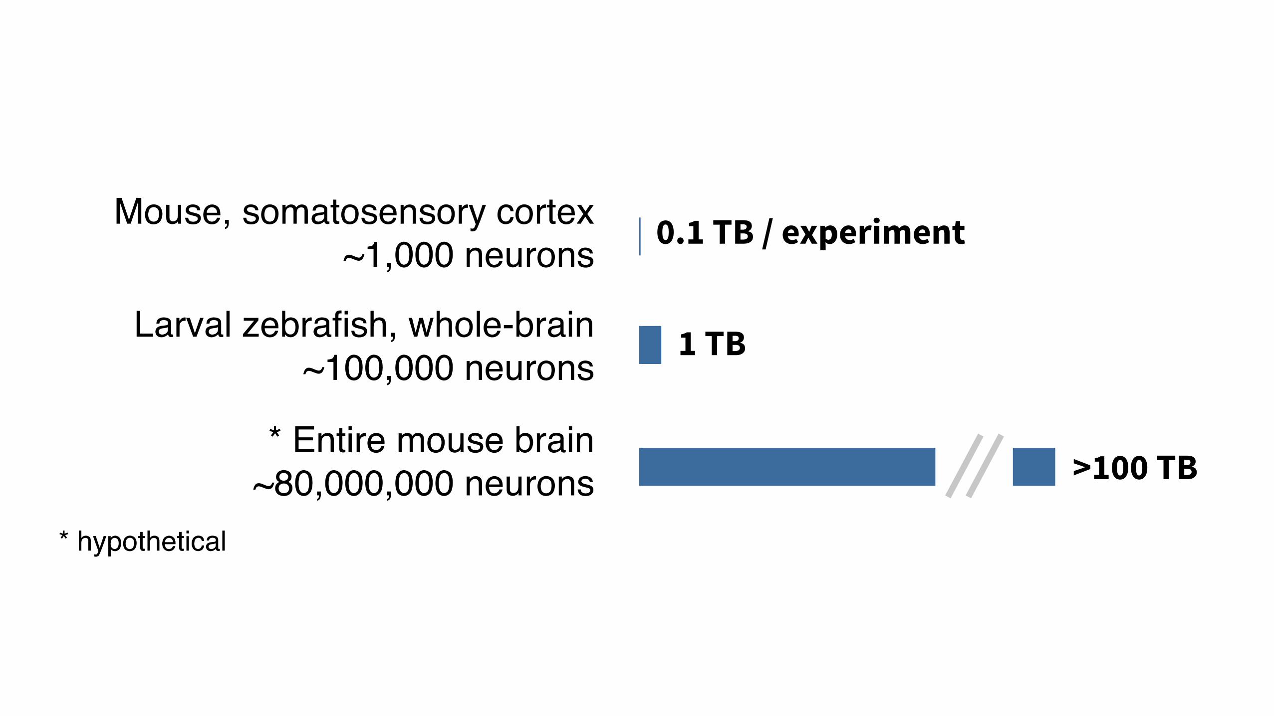
Larval zebrafish, whole-brain~100,000 neurons
1 TB
Mouse, somatosensory cortex~1,000 neurons 0.1 TB / experiment
* Entire mouse brain~80,000,000 neurons >100 TB
* hypothetical

Exploratory Data Analysis

Rawdata
Sharing
Exploring
Visualization
Analysis
Extractedsignals
Interactivefeedback
This is really bigThis is complex

Unsupervised methodsSupervised methods
predict our data
as a function of other data
find structure in the data on its own
y = f(X) f(X)

ClusteringTime
Neu
ral s
igna
ls
Dimensionalityreduction
Regression TuningSummarystatistics
b1 × stim μσ
b2 × motor

Clustering for preprocessing
- Raw data is complex and high-dimensional
- Clustering finds collections of inputs that are similar to one another
- These groups of clusters may be the more meaningful “unit” of measurement

Raw data Clustered data

Clustering to find waveforms associated with individual neurons based on their
traces across multiple electrodes

- Raw data is complex and high-dimensional
- Dimensionality reduction describes the data using a simpler, more compact representation
- This representation may make interesting patterns in the data more clear or easier to see
Dimensionality reduction for insight

Dimensionalityreduction

Yu and Cunningham, 2014
Dimensionalityreduction

Briggman et al., 2005
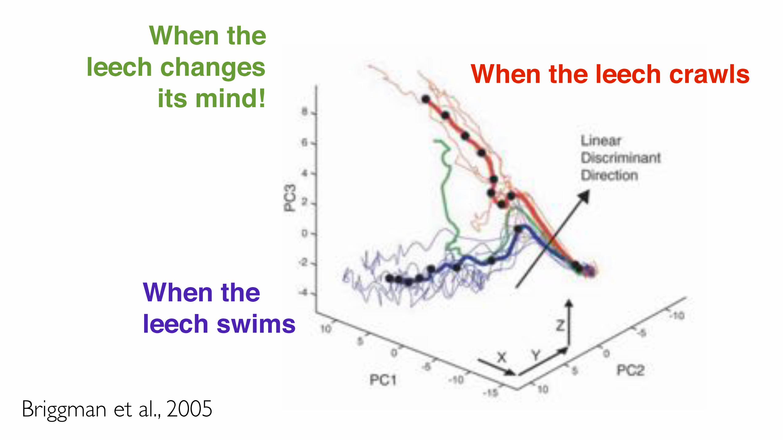
When the leech crawls
When the leech swims
When the leech changes
its mind!
Briggman et al., 2005

Principal Component Analysis (PCA) Overview

To understand a phenomenon we measure various related quantities
If we knew what to measure or how to represent our measurements we might find simple relationships
But in practice we often measure redundant signals, e.g., US and European shoe sizes
We also represent data via the method by which it was gathered, e.g., pixel representation of brain imaging data
Raw data can be Complex, High-dimensional

Issues • Measure redundant signals • Represent data via the method by which it was gathered
Goal: Find a ‘better’ representation for data • To visualize and discover hidden patterns • Preprocessing for supervised task, e.g., feature hashing
Dimensionality Reduction
How do we define ‘better’?

American Size
Euro
pean
Siz
e
E.g., Shoe SizeWe take noisy measurements on European and American scale • Modulo noise, we expect perfect
correlation
How can we do ‘better’, i.e., find a simpler, compact representation? • Pick a direction and project onto
this direction

American Size
Euro
pean
Siz
e
We take noisy measurements on European and American scale • Modulo noise, we expect perfect
correlation
How can we do ‘better’, i.e., find a simpler, compact representation? • Pick a direction and project onto
this direction
E.g., Shoe Size

American Size
Euro
pean
Siz
e
Minimize Euclidean distances between original points and their projections
PCA solution solves this problem!
Goal: Minimize Reconstruction Error

American Size
Euro
pean
Siz
e
x
y
Linear Regression — predict y from x. Evaluate accuracy of predictions (represented by blue line) by vertical distances between points and the line
PCA — reconstruct 2D data via 2D data with single degree of freedom. Evaluate reconstructions (represented by blue line) by Euclidean distances

American Size
Euro
pean
Siz
e
Another Goal: Maximize Variance
To identify patterns we want to study variation across observations
Can we do ‘better’, i.e., find a compact representation that captures variation?

American Size
Euro
pean
Siz
e
Another Goal: Maximize Variance
To identify patterns we want to study variation across observations
Can we do ‘better’, i.e., find a compact representation that captures variation?

American Size
Euro
pean
Siz
e
Another Goal: Maximize Variance
To identify patterns we want to study variation across observations
Can we do ‘better’, i.e., find a compact representation that captures variation? PCA solution finds directions of maximal variance!

PCA Assumptions and Solution

PCA Formulation PCA: find lower-dimensional representation of raw data • is n × d (raw data)• is n × k (reduced representation, PCA ‘scores’)• is d × k (columns are k principal components)• Variance constraints
P
X
Z = XP
Linearity assumption ( ) simplifies problem
Z = XP ≈ ≈
≈
X
P
Z =

σ21 =1n
n�
i=1
�x(i)1
�2Variance of 1st feature (assuming zero mean)
Variance of 1st feature σ21 =1n
n�
i=1
�x(i)1 � μ1
�2
Given n training points with d features:• : matrix storing points• : jth feature for ith point• : mean of jth feature
X � Rn�d
x(i)j
μj

• Symmetric: • Zero → uncorrelated • Large magnitude → (anti) correlated / redundant • → features are the same
σ12 = σ21
Given n training points with d features: • : matrix storing points • : jth feature for ith point • : mean of jth feature
X � Rn�d
x(i)j
μj
σ12 =1n
n�
i=1
x(i)1 x(i)2Covariance of 1st and 2nd
features (assuming zero mean)
σ12 = σ21 = σ22
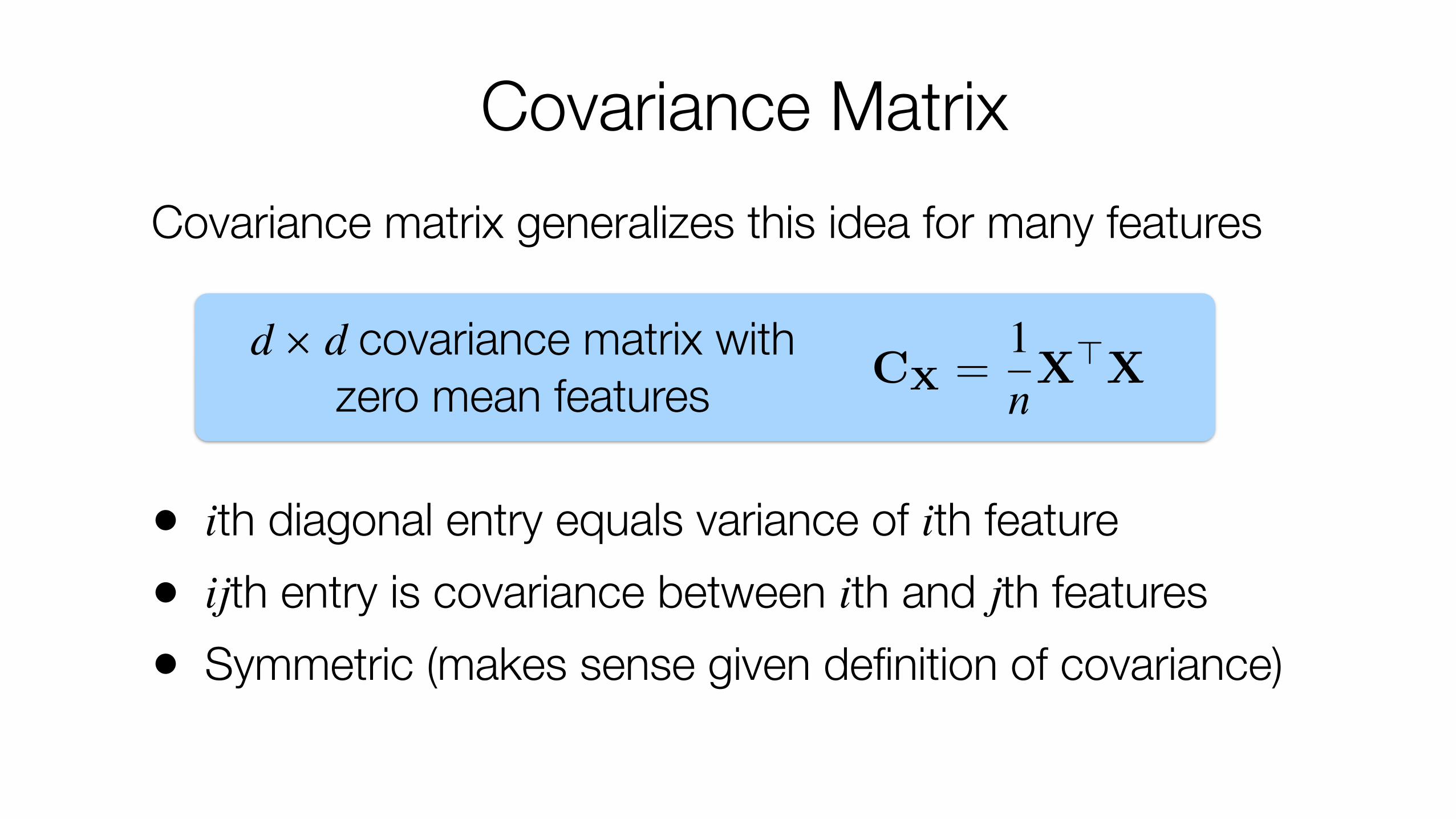
Covariance MatrixCovariance matrix generalizes this idea for many features
• ith diagonal entry equals variance of ith feature• ijth entry is covariance between ith and jth features• Symmetric (makes sense given definition of covariance)
CX =1nX�X
d × d covariance matrix with zero mean features

�2 �1 �13 2 �5
� �
�2 3
�1 2�1 �5
�
� =
�6 99 38
�
XX� X�X
σ21 =1n
n�
i=1
�x(i)1
�2 Variance:

�2 �1 �13 2 �5
� �
�2 3
�1 2�1 �5
�
� =
�6 99 38
�
Covariance: σ12 =1n
n�
i=1
x(i)1 x(i)2
XX� X�X
σ21 =1n
n�
i=1
�x(i)1
�2 Variance:
Dividing by n yields covariance matrix

What constraints make sense in reduced representation?• No feature correlation, i.e., all off-diagonals in are zero• Rank-ordered features by variance, i.e., sorted diagonals of
PCA Formulation PCA: find lower-dimensional representation of raw data • is n × d (raw data) • is n × k (reduced representation, PCA ‘scores’) • is d × k (columns are k principal components) • Variance / Covariance constraints
P
X
Z = XP
CZ
CZ

PCA Formulation PCA: find lower-dimensional representation of raw data • is n × d (raw data) • is n × k (reduced representation, PCA ‘scores’) • is d × k (columns are k principal components) • Variance / Covariance constraints
P
X
Z = XP
equals the top k eigenvectors of CXP ≈ ≈
≈
X
P
Z =

PCA Solution All covariance matrices have an eigendecomposition • (eigendecomposition) • is d × d (column are eigenvectors, sorted by their eigenvalues) • is d × d (diagonals are eigenvalues, off-diagonals are zero)
The d eigenvectors are orthonormal directions of max variance • Associated eigenvalues equal variance in these directions • 1st eigenvector is direction of max variance (variance is )
U
Λ
CX = UΛU�
λ1
In lab, we’ll use the eigh function from numpy.linalg
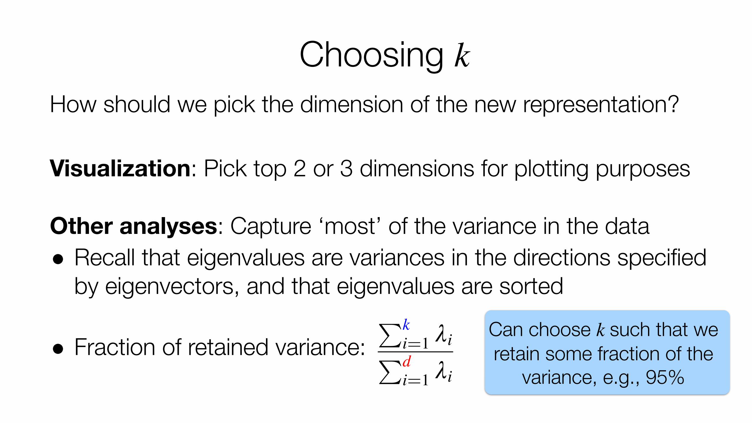
Choosing kHow should we pick the dimension of the new representation?
Visualization: Pick top 2 or 3 dimensions for plotting purposes
Other analyses: Capture ‘most’ of the variance in the data • Recall that eigenvalues are variances in the directions specified
by eigenvectors, and that eigenvalues are sorted
• Fraction of retained variance:�k
i=1 λi�di=1 λi
Can choose k such that we retain some fraction of the
variance, e.g., 95%

Other Practical TipsPCA assumptions (linearity, orthogonality) not always appropriate • Various extensions to PCA with different underlying
assumptions, e.g., manifold learning, Kernel PCA, ICA
Centering is crucial, i.e., we must preprocess data so that all features have zero mean before applying PCA
PCA results dependent on scaling of data • Data is sometimes rescaled in practice before applying PCA

PCA Algorithm

Orthogonal and Orthonormal VectorsOrthogonal vectors are perpendicular to each other• Equivalently, their dot product equals zero• and , but c isn’t orthogonal to others
Orthonormal vectors are orthogonal and have unit norm • a are b are orthonormal, but b are d are not orthonormal
a =�1 0
��b =
�0 1
��c =
�1 1
��d =
�2 0
��
a�b = 0 d�b = 0

PCA Iterative Algorithm k = 1: Find direction of max variance, project onto this direction • Locations along this direction are the new 1D representation
American Size
Euro
pean
Siz
e
More generally, for i in {1, …, k}:• Find direction of max variance that is
orthonormal to previously selected directions, project onto this direction
• Locations along this direction are the ith feature in new representation

PCA Derivation (Optional)

EigendecompositionAll covariance matrices have an eigendecomposition• (eigendecomposition)• is d × d (column are eigenvectors, sorted by their eigenvalues)• is d × d (diagonals are eigenvalues, off-diagonals are zero)Eigenvector / Eigenvalue equation:• By definition (unit norm)
• Example:
U
Λ
CX = UΛU�
Cxu = λuu�u = 1
�1 00 1
� �10
�=
�10
�⟹ eigenvector:
eigenvalue: λ = 1u =
�1 0
��

PCA Formulation
PCA: find lower-dimensional representation of raw data
• is n × d (raw data)
• is n × k (reduced representation, PCA ‘scores’)
• is d × k (columns are k principal components)
• Variance / Covariance constraints
P
X
Z = XP
≈ ≈
≈
X
P
Z =

PCA Formulation, k = 1
Goal: Maximizes variance, i.e., maxp
||z||22
σ2 =1n
n�
i=1
�z(i)
�2= ||z||22 = ||Xp||22
σ2z ||p||2 = 1where
σ2z
PCA: find one-dimensional representation of raw data • is n × d (raw data) • is n × 1 (reduced representation, PCA ‘scores’) • is d × 1 (columns are k principal components) • Variance constraint
X
p
z = Xp

Relationship between Euclidean distance and dot product
z = XpDefinition:
Transpose property: ; associativity of multiply(Xp)� = p�X�
Definition: CX =1nX�X
σ2z = ||z||22= z�z
= (Xp)�(Xp)
= p�X�Xp
= np�Cxp
Goal: Maximizes variance, i.e., maxp
||z||22σ2z ||p||2 = 1where
maxp
p�CxpRestated Goal: ||p||2 = 1where

Recall eigenvector / eigenvalue equation:• By definition , and thus • But this is the expression we’re optimizing, and thus maximal
variance achieved when is top eigenvector of
Similar arguments can be used for k > 1
maxp
p�CxpRestated Goal: ||p||2 = 1where
Cxu = λu
u�u = 1 u�Cxu = λ
CXp
Connection to Eigenvectors

Distributed PCA

Computing PCA SolutionGiven: n × d matrix of uncentered raw dataGoal: Compute k ≪ d dimensional representation
Step 1: Center DataStep 2: Compute Covariance or Scatter Matrix• versus Step 3: EigendecompositionStep 4: Compute PCA Scores
CX =1nX�XCX =
1nX�X
≈ ≈
≈
X
P
Z =

PCA at ScaleCase 1: Big n and Small d • O(d2) local storage, O(d3) local computation, O(dk)
communication • Similar strategy as closed-form linear regression
Case 2: Big n and Big d• O(dk + n) local storage, computation;
O(dk + n) communication • Iterative algorithm
≈ ≈
≈
X
P
Z =

Example: n = 6; 3 workers
O(nd) Distributed Storageworkers: x(1)
x(5)
x(3)
x(4)
x(2)
x(6)
( )reduce:�
x(i)
O(d) Local Storage O(d) Local Computation
O(d) Communicationm =
1n
m
Step 1: Center Data
• Compute d feature means,
• Communicate to all workers
m � Rd
m
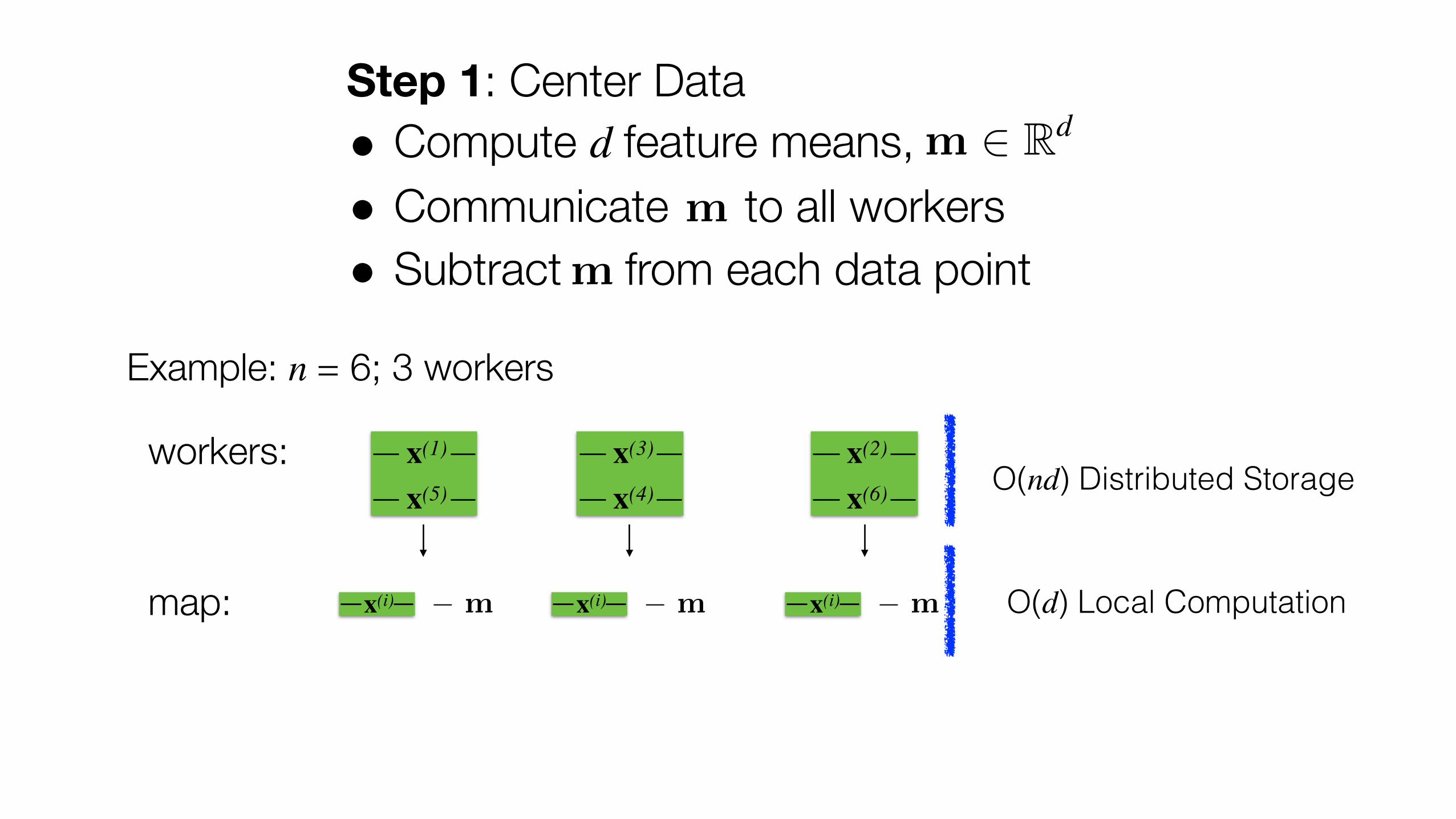
Example: n = 6; 3 workers
O(nd) Distributed Storageworkers: x(1)
x(5)
x(3)
x(4)
x(2)
x(6)
Step 1: Center Data • Compute d feature means, • Communicate to all workers • Subtract from each data point
m � Rd
m
map: x(i) � m x(i) � m x(i) � m O(d) Local Computation
m

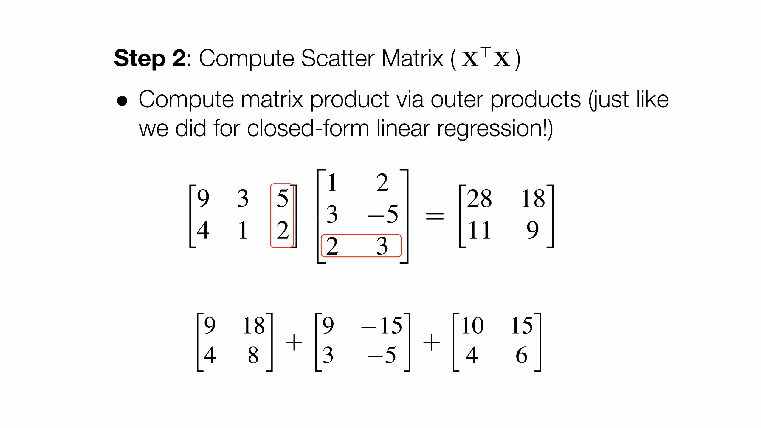
Step 2: Compute Scatter Matrix ( ) • Compute matrix product via outer products (just like
we did for closed-form linear regression!)
�9 3 54 1 2
� �
�1 23 �52 3
�
� =
�28 1811 9
�
�9 184 8
�+
�9 �153 �5
�+
�10 154 6
�
CX =1nX�X

Step 2: Compute Scatter Matrix ( ) • Compute matrix product via outer products (just like
we did for closed-form linear regression!)
�9 3 54 1 2
� �
�1 23 �52 3
�
� =
�28 1811 9
�
�9 184 8
�+
�9 �153 �5
�+
�10 154 6
�
CX =1nX�X
Step 2: Compute Scatter Matrix ( ) • Compute matrix product via outer products (just like
we did for closed-form linear regression!)
�9 3 54 1 2
� �
�1 23 �52 3
�
� =
�28 1811 9
�
�9 184 8
�+
�9 �153 �5
�+
�10 154 6
�
CX =1nX�X

Example: n = 6; 3 workers
x(1)
…
x(1) …
d
n
n
d
x(2)
x(n)
x(2)
x(n)
=n�
i=1
x(i)
x(i)
O(nd) Distributed Storageworkers: x(1)
x(5)
x(3)
x(4)
x(2)
x(6)
X�X =
map:
x(i)
x(i)x(
i)x(i)
x(i)
x(i) O(d2) Local Storage O(nd2) Distributed Computation
reduce:�
x(i)
x(i) O(d2) Local Storage O(d2) Local Computation

Example: n = 6; 3 workers
O(nd) Distributed Storageworkers: x(1)
x(5)
x(3)
x(4)
x(2)
x(6)
map:
x(i)
x(i)x(
i)x(i)
x(i)
x(i) O(d2) Local Storage O(nd2) Distributed Computation
reduce:�
x(i)
x(i)O(d2) Local Storage O(d3) Local Computation
O(dk) Communication
Step 3: Eigendecomposition • Perform locally since d is small • Communicate k principal components ( )
to workers
eigh( )P
P � Rd�k

Example: n = 6; 3 workers
O(nd) Distributed Storageworkers: x(1)
x(5)
x(3)
x(4)
x(2)
x(6)
Step 4: Compute PCA Scores • Multiply each point by principal components,
map: x(i) O(dk) Local Computation
P
p(1)
p(2) x(i)p(1)
p(2) x(i)p(1)
p(2)

Distributed PCA, Part II (Optional)

PCA at ScaleCase 1: Big n and Small d • O(d2) local storage, O(d3) local computation, O(dk)
communication • Similar strategy as closed-form linear regression
Case 2: Big n and Big d• O(dk + n) local storage, computation;
O(dk + n) communication • Iterative algorithm
≈ ≈
≈
X
P
Z =

An Iterative ApproachWe can use algorithms that rely on a sequence of matrix-vector products to compute top k eigenvectors ( ) • E.g., Krylov subspace or random projection methods
Krylov subspace methods (used in MLlib) iteratively compute for some provided by the method • Requires O(k) passes over the data and O(dk) local storage • We don’t need to compute the covariance matrix!
X�Xv v � Rd
P
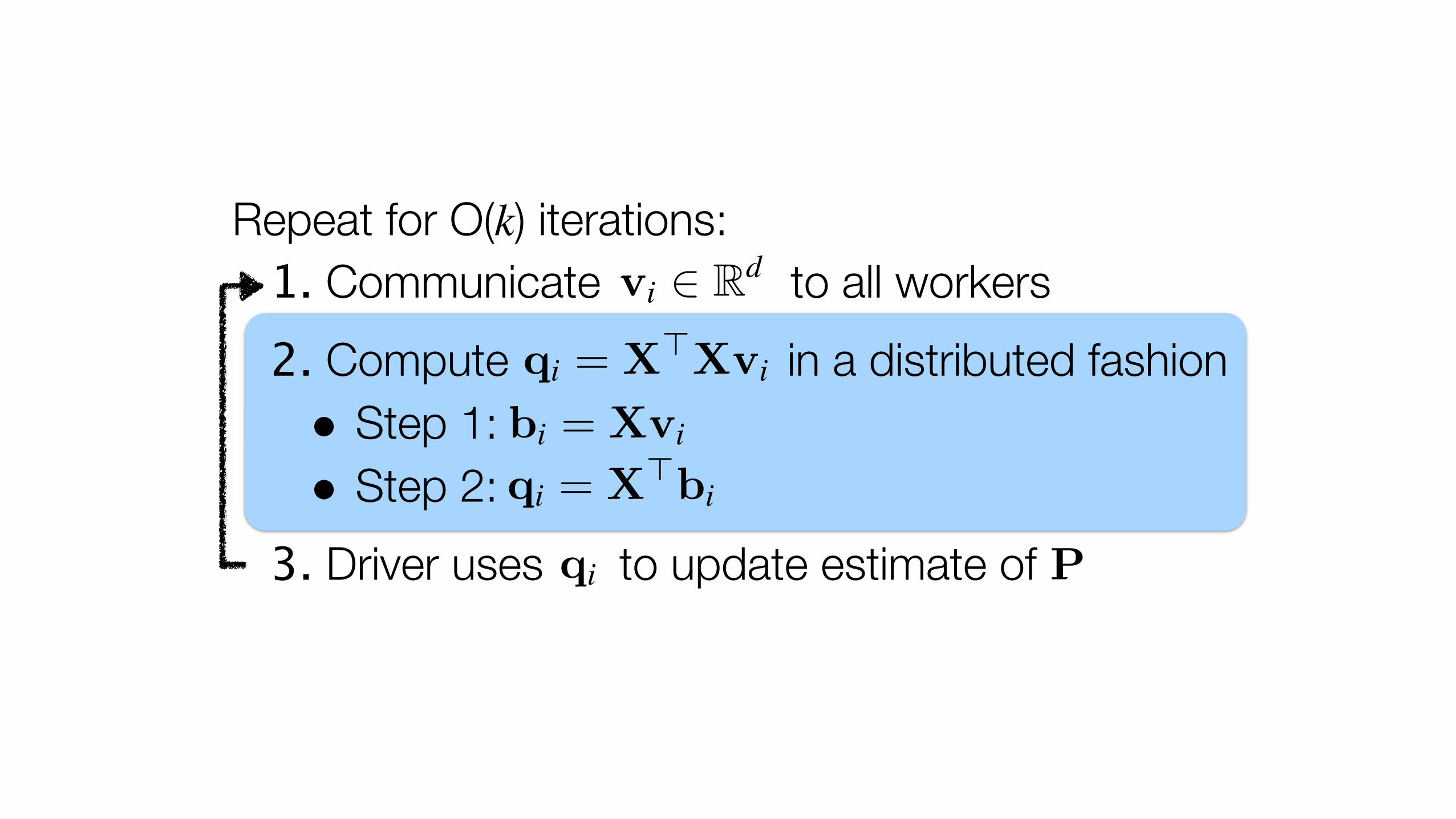
Repeat for O(k) iterations: 1. Communicate to all workers 2. Compute in a distributed fashion • Step 1: • Step 2:
3. Driver uses to update estimate of
vi � Rd
qi = X�Xvi
bi = Xvi
qi = X�bi
Pqi = X�Xvi

Example: n = 6; 3 workers
O(nd) Distributed Storageworkers: x(1)
x(5)
x(3)
x(4)
x(2)
x(6)
O(n) Local Storage O(n) Local Computation
O(n) Communication
map:
x(j)
vi O(d) Local Storage O(nd) Distributed Computationx(
j)
vi
x(j)
vi
reduce: bi = [v�x(1) . . . v�x(n)]�
bi
Compute in a distributed fashion • : each component is dot product, then concatenate
qi = X�Xvi
bi = Xvi

Example: n = 6; 3 workers
O(nd) Distributed Storageworkers: x(1)
x(5)
x(3)
x(4)
x(2)
x(6)
Compute in a distributed fashion • : each component is dot product, then concatenate
• : sum of rescaled data points
qi = X�Xvi
bi = Xvi
qi = X�bi qi =n�
j=1
bijx(j)
map:
x(j)bij ⨉
O(n) Local Storage O(nd) Distributed Computationx(
j)bij ⨉ x(j)bij ⨉
reduce:O(d) Local Storage O(d) Local Computation
O(d) Communication
�x(
j)bij ⨉qi =

Lab Preview

Which areas are active at which times?
Which neuronal populations are activated by different directions of the stimulus?
Vladimirov et al., 2014

Find representations of data that reveal how responses are organized across space and time
Collection of neural time series
Given
Goal

Swim
stre
ngth
Res
pons
e
Cycle average
PCA
0
20 sec
0.5
dim 1 di
m 2
Visualize


