
CS 229br: Advanced Topics in the theory of machine learning
Boaz Barak
Join slack team and sign in on your devices!
Ankur MoitraMIT 18.408
Yamini BansalOfficial TF
Dimitris KalimerisUnofficial TF
Gal KaplunUnofficial TF
Preetum NakkiranUnofficial TF

What is learning?
𝑓 World

What is learning?
𝑓 World
What is deep learning?

𝑓 World
OPT
ℒ
ℱdata 𝑓
Benchmark
100
0
𝑓
ℒ ℝ
data
𝑓
OOD, domain shift,
robustness, fairness, ..
Generalization,..
Optimization,..


God’s view:
f = argmax𝑓 𝔼 (𝑓) data ]
f = argmax𝑓 𝔼[ (𝑓 ↔ 𝑤) ]
𝑤 ∼ 𝑊|data
Perfect A Perfect B ≠ Approx A Approx B

This seminar• Taste of research results, questions, experiments, and more
• Goal: Get to state of art research:
• Background and language
• Reading and reproducing papers
• Trying out extensions
• Very experimental and “rough around the edges”
• A lot of learning on your own and from each other
• Hope: Very interactive – in lectures and on slack
CS 229br: Survey of very recent research directions, emphasis on experiments
MIT 18.408: Deeper coverage of foundations, emphasis on theory

Student expectationsNot set in stone but will include:
• Pre-reading before lectures
• Scribe notes / blog posts (adding proofs and details)
• Applied problem sets (replicating papers or mini versions thereof, exploring)
Note: Lectures will not teach practical skills – rely on students to pick up using
suggested tutorials, other resources, and each other.
Unofficial TFs happy to answer questions!
• Some theoretical problem sets.
• Might have you grade each other’s work
• Projects – self chosen and directed.
Grading: We’ll figure out some grade – hope that’s not your loss function ☺
HW0 on
slack

Rest of today’s lecture:
Blitz through classical learning theory
• Special cases, mostly one dimension
• “Proofs by picture”

Part I: Convexity & Optimization
Convexity
𝑥 𝑦
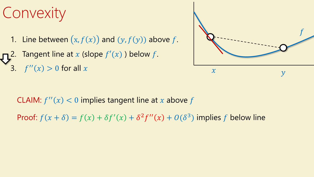
𝑓1. Line between x, 𝑓 𝑥 and (𝑦, 𝑓 𝑦 ) above 𝑓.
2. Tangent line at 𝑥 (slope 𝑓′(𝑥) ) below 𝑓.
3. 𝑓′′ 𝑥 > 0 for all 𝑥
CLAIM: 𝑓′′ 𝑥 < 0 implies tangent line at 𝑥 above 𝑓
Proof: 𝑓 𝑥 + 𝛿 = 𝑓 𝑥 + 𝛿𝑓′ 𝑥 + 𝛿2𝑓′′ 𝑥 + 𝑂(𝛿3) implies 𝑓 below line
Convexity
𝑥 𝑦
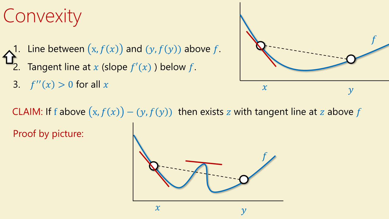
𝑓1. Line between x, 𝑓 𝑥 and (𝑦, 𝑓 𝑦 ) above 𝑓.
2. Tangent line at 𝑥 (slope 𝑓′(𝑥) ) below 𝑓.
3. 𝑓′′ 𝑥 > 0 for all 𝑥
𝑥 𝑦
𝑓
CLAIM: If f above x, 𝑓 𝑥 − (𝑦, 𝑓 𝑦 ) then exists 𝑧 with tangent line at 𝑧 above 𝑓
Proof by picture:
Gradient Descent
𝑥𝑡 𝑦
𝑓
𝑥𝑡+1
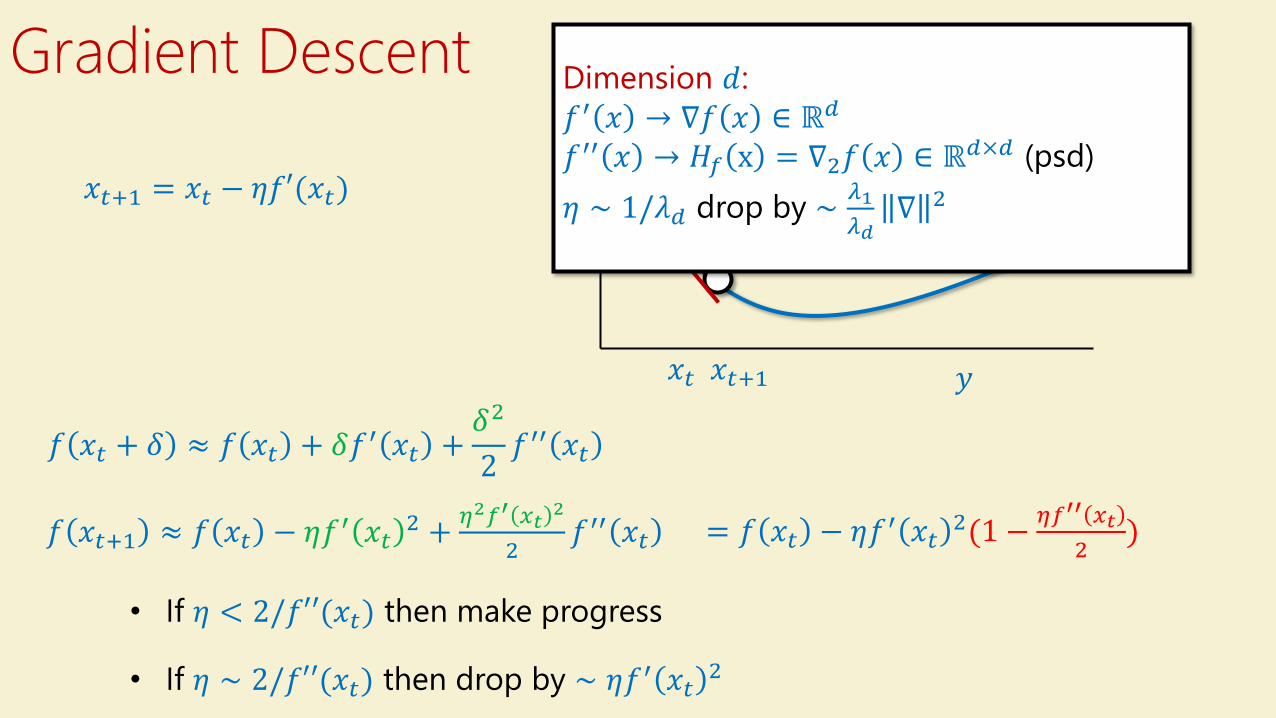
𝑥𝑡+1 = 𝑥𝑡 − 𝜂𝑓′(𝑥𝑡)
𝑓 𝑥𝑡 + 𝛿 ≈ 𝑓 𝑥𝑡 + 𝛿𝑓′ 𝑥𝑡 +𝛿2
2𝑓′′ 𝑥𝑡
𝑓 𝑥𝑡+1 ≈ 𝑓 𝑥𝑡 − 𝜂𝑓′ 𝑥𝑡2 +
𝜂2𝑓′ 𝑥𝑡2
2𝑓′′ 𝑥𝑡
• If 𝜂 < 2/𝑓′′(𝑥𝑡) then make progress
• If 𝜂 ∼ 2/𝑓′′(𝑥𝑡) then drop by ∼ 𝜂𝑓′ 𝑥𝑡2
Dimension 𝑑:
𝑓′ 𝑥 → ∇𝑓 𝑥 ∈ ℝ𝑑
𝑓′′ 𝑥 → 𝐻𝑓 x = ∇2𝑓 𝑥 ∈ ℝ𝑑×𝑑 (psd)
𝜂 ∼ 1/𝜆𝑑 drop by ∼𝜆1
𝜆𝑑∇ 2
= 𝑓 𝑥𝑡 − 𝜂𝑓′ 𝑥𝑡2(1 −
𝜂𝑓′′ 𝑥𝑡
2)
Stochastic Gradient Descent
𝑥𝑡 𝑦
𝑓
𝑥𝑡+1
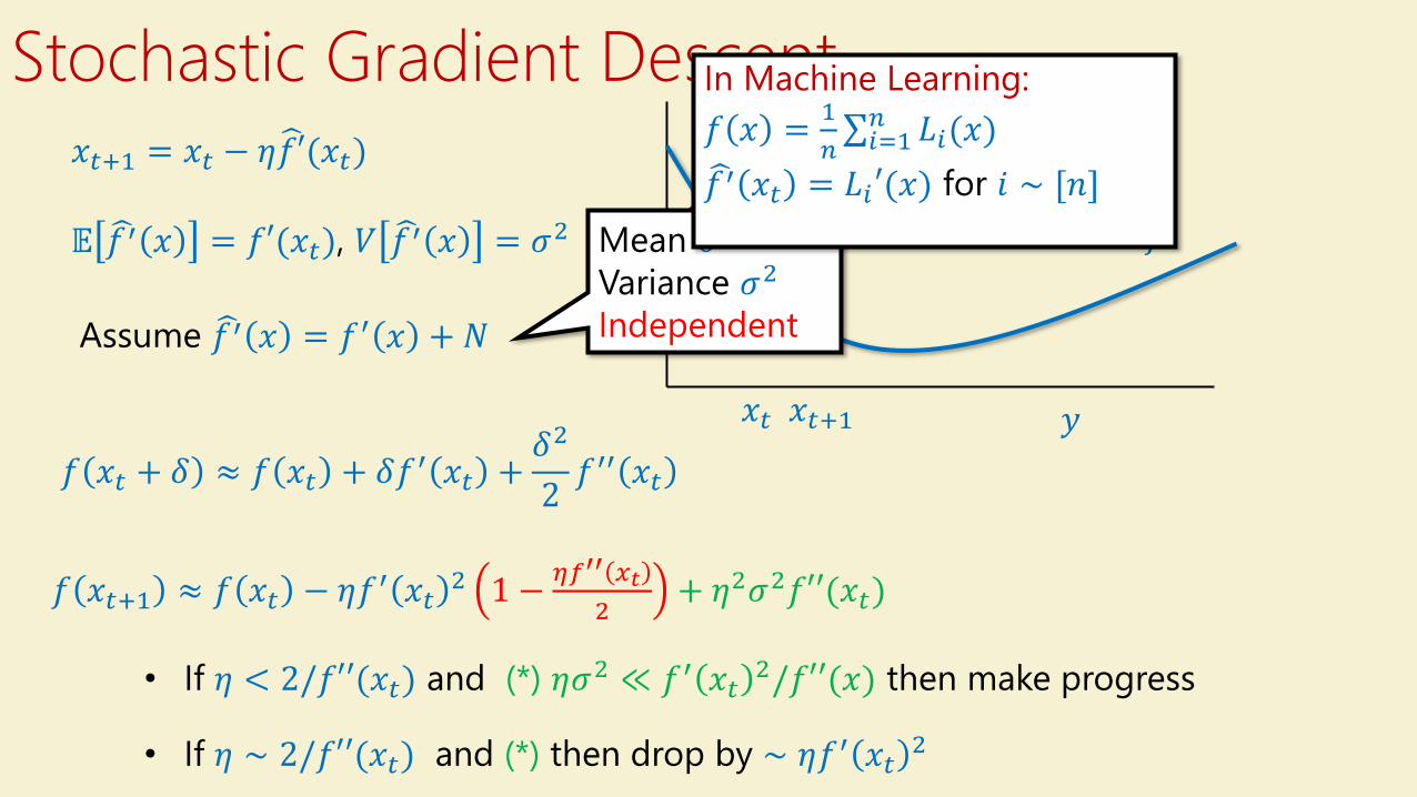
𝑥𝑡+1 = 𝑥𝑡 − 𝜂𝑓′(𝑥𝑡)
𝑓 𝑥𝑡 + 𝛿 ≈ 𝑓 𝑥𝑡 + 𝛿𝑓′ 𝑥𝑡 +𝛿2
2𝑓′′ 𝑥𝑡
𝑓 𝑥𝑡+1 ≈ 𝑓 𝑥𝑡 − 𝜂𝑓′ 𝑥𝑡2 1 −
𝜂𝑓′′ 𝑥𝑡
2+ 𝜂2𝜎2𝑓′′(𝑥𝑡)
• If 𝜂 < 2/𝑓′′(𝑥𝑡) and (*) 𝜂𝜎2 ≪ 𝑓′ 𝑥𝑡2/𝑓′′(𝑥) then make progress
• If 𝜂 ∼ 2/𝑓′′(𝑥𝑡) and (*) then drop by ∼ 𝜂𝑓′ 𝑥𝑡2
𝔼 𝑓′ 𝑥 = 𝑓′(𝑥𝑡), 𝑉 𝑓′ 𝑥 = 𝜎2
Assume 𝑓′ 𝑥 = 𝑓′ 𝑥 + 𝑁
Mean 0Variance 𝜎2
Independent
In Machine Learning:
𝑓 𝑥 =1
𝑛σ𝑖=1𝑛 𝐿𝑖(𝑥)
𝑓′ 𝑥𝑡 = 𝐿𝑖′(𝑥) for 𝑖 ∼ [𝑛]

Part II: Generalization
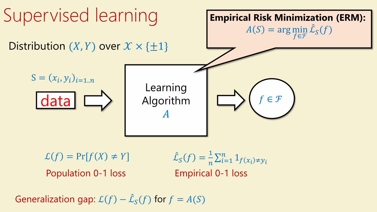
Distribution (𝑋, 𝑌) over 𝒳 × {±1}
Supervised learning
Learning
Algorithm
𝐴data
S = 𝑥𝑖 , 𝑦𝑖 𝑖=1..𝑛
𝑓 ∈ ℱ
ℒ 𝑓 = Pr[𝑓 𝑋 ≠ 𝑌] መℒ𝑆 𝑓 =1
𝑛σ𝑖=1𝑛 1𝑓 𝑥𝑖 ≠𝑦𝑖
Population 0-1 loss Empirical 0-1 loss
Generalization gap: ℒ 𝑓 − መℒ𝑆(𝑓) for 𝑓 = 𝐴(𝑆)
Empirical Risk Minimization (ERM):
𝐴 𝑆 = argmin𝑓∈ℱ
መℒ𝑆(𝑓)

Bias Variance TradeoffLearning
Algorithm
𝐴S = 𝑥𝑖 , 𝑦𝑖 𝑖=1..𝑛 𝑓 ∈ ℱ
Empirical Risk Minimization (ERM):
𝐴 𝑆 = argmin𝑓∈ℱ
መℒ𝑆(𝑓)
ℒ 𝑓 = Pr[𝑓 𝑋 ≠ 𝑌] መℒ𝑆 𝑓 =1
𝑛σ𝑖=1𝑛 1𝑓 𝑥𝑖 ≠𝑦𝑖Population 0-1 loss Empirical 0-1 loss
Assume ℱ𝐾 = { 𝑓1, … , 𝑓𝐾} , መℒ 𝑓𝑖 = ℒ 𝑓𝑖 +𝑁(0, 1/𝑛)
𝐾 (log scale)
bias variance
Lo
ss
∼log 𝐾
𝑛?
∼ log𝐾 −𝛼 ??
Can prove:
GAP ≤ 𝑂log |ℱ|
𝑛

Bias Variance TradeoffLearning
Algorithm
𝐴S = 𝑥𝑖 , 𝑦𝑖 𝑖=1..𝑛 𝑓 ∈ ℱ
Empirical Risk Minimization (ERM):
𝐴 𝑆 = argmin𝑓∈ℱ
መℒ𝑆(𝑓)
ℒ 𝑓 = Pr[𝑓 𝑋 ≠ 𝑌] መℒ𝑆 𝑓 = σ𝑖=1𝑛 1𝑓 𝑥𝑖 ≠𝑦𝑖
Population 0-1 loss Empirical 0-1 loss
Assume ℱ𝐾 = { 𝑓1, … , 𝑓𝐾} , መℒ 𝑓𝑖 = ℒ 𝑓𝑖 +𝑁(0, 1/𝑛)
𝐾 (log scale)
bias variance
Lo
ss
∼log 𝐾
𝑛?
∼ log𝐾 −𝛼 ??
Can prove:
GAP ≤ 𝑂log |ℱ|
𝑛
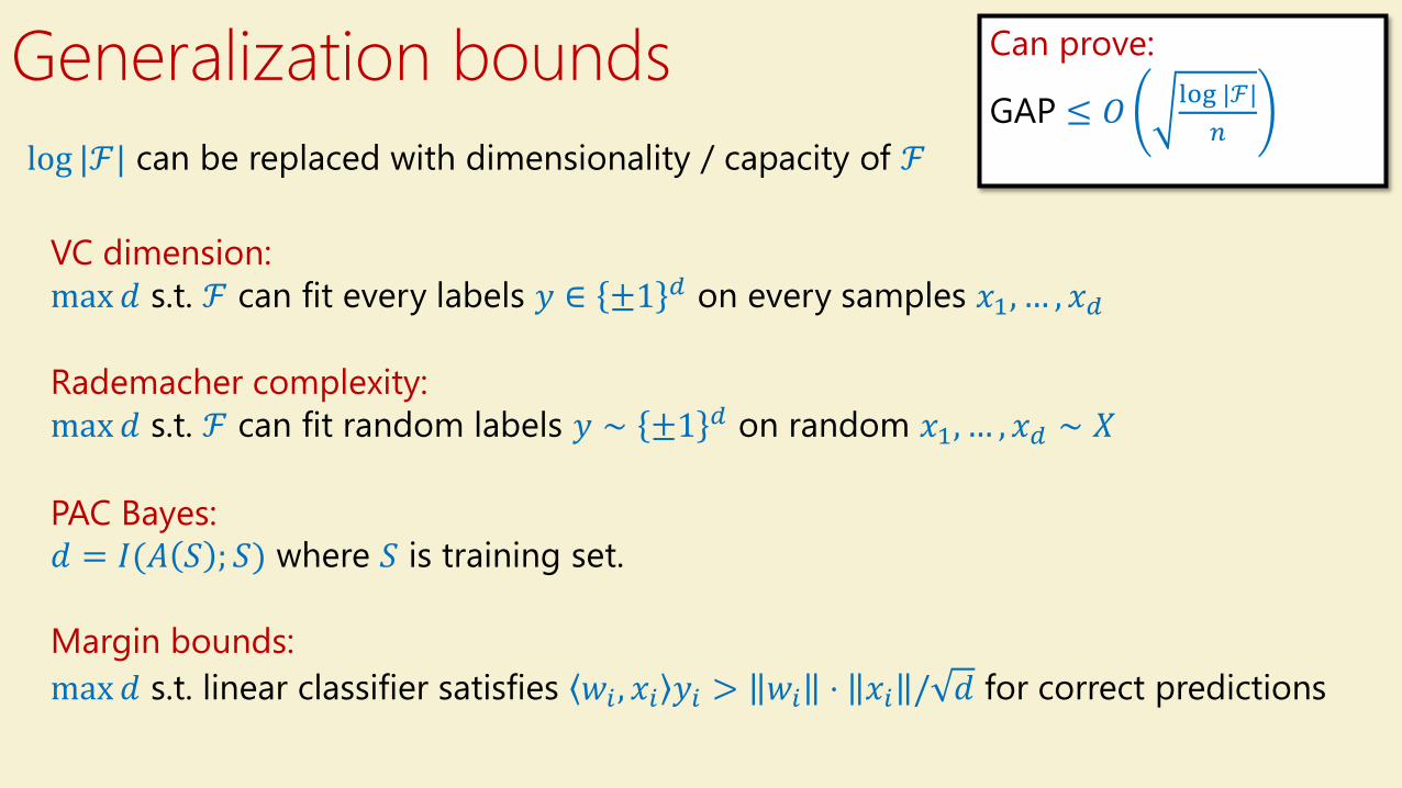
Generalization bounds Can prove:
GAP ≤ 𝑂log |ℱ|
𝑛log |ℱ| can be replaced with dimensionality / capacity of ℱ
VC dimension:
max 𝑑 s.t. ℱ can fit every labels 𝑦 ∈ ±1 𝑑 on every samples 𝑥1, … , 𝑥𝑑
Rademacher complexity:
max 𝑑 s.t. ℱ can fit random labels 𝑦 ∼ ±1 𝑑 on random 𝑥1, … , 𝑥𝑑 ∼ 𝑋
PAC Bayes:
𝑑 = 𝐼(𝐴 𝑆 ; 𝑆) where 𝑆 is training set.
Margin bounds:
max 𝑑 s.t. linear classifier satisfies 𝑤𝑖 , 𝑥𝑖 𝑦𝑖 > 𝑤𝑖 ⋅ 𝑥𝑖 / 𝑑 for correct predictions
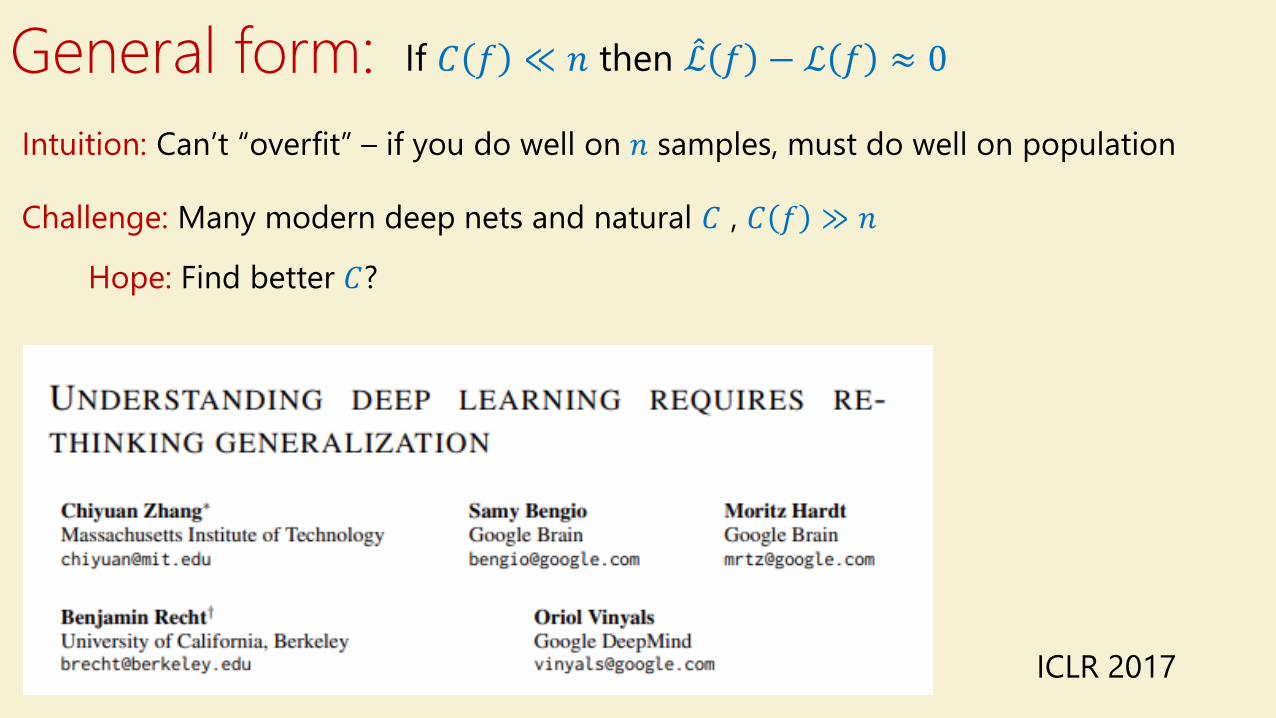
General form: If 𝐶 𝑓 ≪ 𝑛 then መℒ 𝑓 − ℒ 𝑓 ≈ 0
Challenge: Many modern deep nets and natural 𝐶 , 𝐶 𝑓 ≫ 𝑛
Intuition: Can’t “overfit” – if you do well on 𝑛 samples, must do well on population
Hope: Find better 𝐶?
ICLR 2017

General form: If 𝐶 𝑓 ≪ 𝑛 then መℒ 𝑓 − ℒ 𝑓 ≈ 0
Challenge: Many modern deep nets and natural 𝐶 , 𝐶 𝑓 ≫ 𝑛
Intuition: Can’t “overfit” – if you do well on 𝑛 samples, must do well on population
Hope: Find better 𝐶?
Classifier Train Test
Wide ResNet1
100% 92%
ResNet 182 100% 87%
Myrtle3 100% 86%
Performance on CIFAR-10 Performance on noisy CIFAR-10:*
Train Test
100% 10%
100% 10%
100% 10%
1 Zagoruyko-Komodakis’16 2 He-Zhang-Ren-Sun’15 3 Page ’19
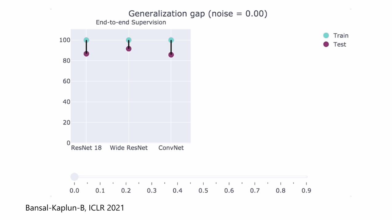
Bansal-Kaplun-B, ICLR 2021

“Double descent”
Belkin, Hsu, Ma, Mandal, PNAS 2019.
Nakkiran-Kaplun-Bansal-Yang-B-Sutskever, ICLR 2020

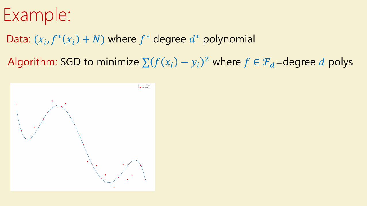
Example:
Data: (𝑥𝑖 , 𝑓∗ 𝑥𝑖 + 𝑁) where 𝑓∗ degree 𝑑∗ polynomial
Algorithm: SGD to minimize σ 𝑓 𝑥𝑖 − 𝑦𝑖2 where 𝑓 ∈ ℱ𝑑=degree 𝑑 polys
Cartoon:
𝑑∗ 𝑛
degree 𝑑 = 𝐶(ℱ)
Lo
ss/e
rro
r
Test
Train
Example:
Data: (𝑥𝑖 , 𝑓∗ 𝑥𝑖 + 𝑁) where 𝑓∗ degree 𝑑∗ polynomial
Algorithm: SGD to minimize σ 𝑓 𝑥𝑖 − 𝑦𝑖2 where 𝑓 ∈ ℱ𝑑=degree 𝑑 polys

Example:
Data: (𝑥𝑖 , 𝑓∗ 𝑥𝑖 + 𝑁) where 𝑓∗ degree 𝑑∗ polynomial
Algorithm: SGD to minimize σ 𝑓 𝑥𝑖 − 𝑦𝑖2 where 𝑓 ∈ ℱ𝑑=degree 𝑑 polys

Part III: Approximation and Representation
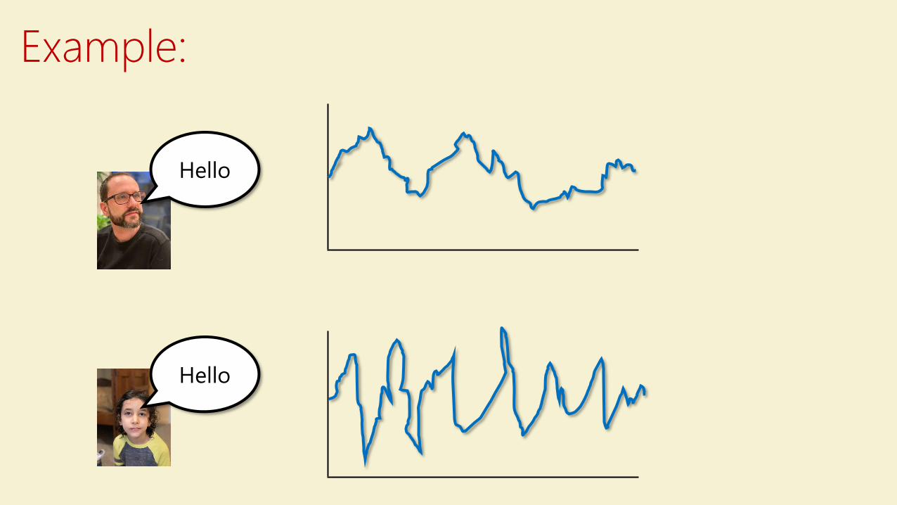
Hello
Hello
Example:
Example:
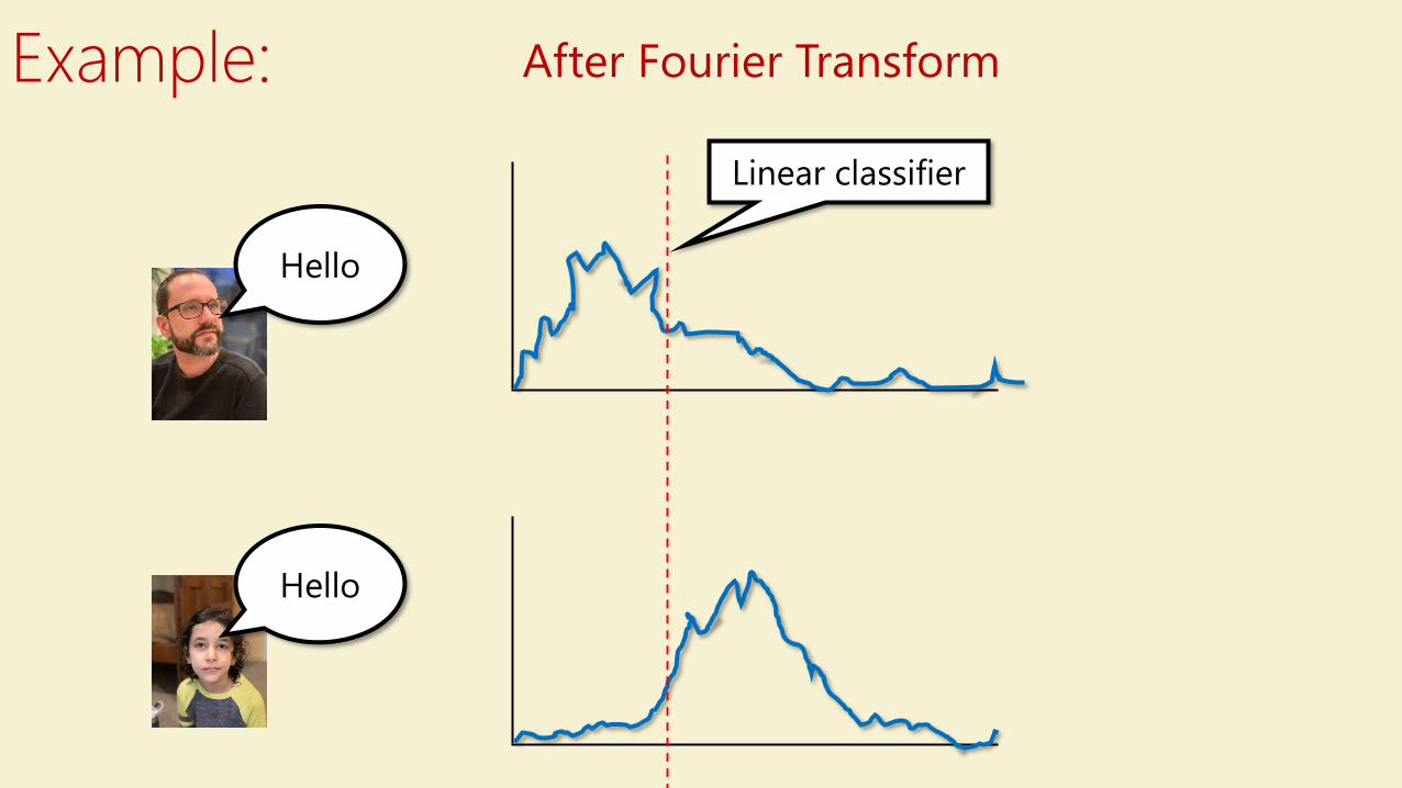
Hello
Hello
After Fourier Transform
Linear classifier

Fourier Transform
Every continuous 𝑓: 0,1 → ℝ can be arbitrarily approximated
by 𝑔 of form
𝑔 𝑥 = σ𝛼𝑗𝑒−2𝜋𝑖 𝛽𝑗𝑥
For some natural data, representation 𝜑 is “nice”
(e.g. sparse, linearly separable,…)
Tasks become simpler after transformation 𝑥 → 𝜑(𝑥)
i.e., 𝑓 ≈ linear in 𝜑1 𝑥 ,… , 𝜑𝑁(𝑥) where 𝜑𝑗 𝑥 = 𝑒−2𝜋𝑖 𝛽𝑗𝑥
𝜑:ℝ → ℝ𝑁 embedding
න0
1
|𝑓 − 𝑔| < 𝜖

𝜑 𝑥, 𝑦 = (𝑥𝑦, 𝑥2, 𝑦2)
Xavier Bourret Sicotte, https://xavierbourretsicotte.github.io/Kernel_feature_map.html
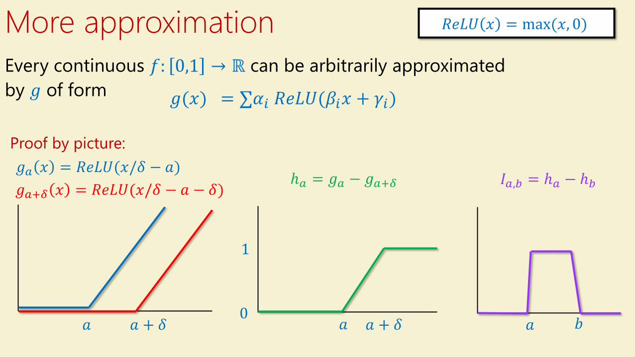
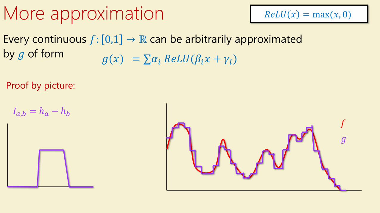
More approximation
𝑔(𝑥) = σ𝛼𝑖 𝑅𝑒𝐿𝑈(𝛽𝑖𝑥 + 𝛾𝑖)
Proof by picture:
𝑅𝑒𝐿𝑈 𝑥 = max(𝑥, 0)
𝑎 𝑎 + 𝛿
𝑔𝑎 𝑥 = 𝑅𝑒𝐿𝑈(𝑥/𝛿 − 𝑎)
𝑔𝑎+𝛿 𝑥 = 𝑅𝑒𝐿𝑈(𝑥/𝛿 − 𝑎 − 𝛿)
𝑎 𝑎 + 𝛿0
1
ℎ𝑎 = 𝑔𝑎 − 𝑔𝑎+𝛿 𝐼𝑎,𝑏 = ℎ𝑎 − ℎ𝑏
Every continuous 𝑓: 0,1 → ℝ can be arbitrarily approximated
by 𝑔 of form
𝑎 𝑏
More approximation
𝑔(𝑥) = σ𝛼𝑖 𝑅𝑒𝐿𝑈(𝛽𝑖𝑥 + 𝛾𝑖)
Proof by picture:
𝑅𝑒𝐿𝑈 𝑥 = max(𝑥, 0)
𝐼𝑎,𝑏 = ℎ𝑎 − ℎ𝑏
Every continuous 𝑓: 0,1 → ℝ can be arbitrarily approximated
by 𝑔 of form
𝑓
𝑔

Higher dimension
𝐼(𝑥)
𝐽 1,0 𝑥, 𝑦 = 𝐼 𝑥
𝑟 𝑥 = max( 𝛼, 𝑥 + 𝛽, 0) , 𝑑 + 1 parameters

Higher dimension
𝐼(𝑥)
𝐽 1,0 𝑥, 𝑦 = 𝐼 𝑥
𝑟 𝑥 = max( 𝛼, 𝑥 + 𝛽, 0) , 𝑑 + 1 parameters
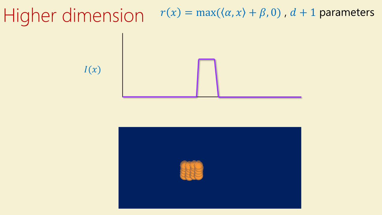
Higher dimension
𝐼(𝑥)
𝑟 𝑥 = max( 𝛼, 𝑥 + 𝛽, 0) , 𝑑 + 1 parameters
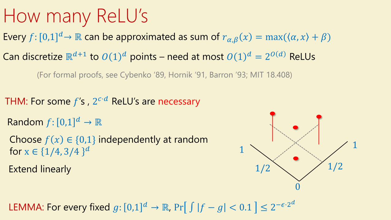
How many ReLU’sEvery 𝑓: [0,1]𝑑→ ℝ can be approximated as sum of 𝑟𝛼,𝛽 𝑥 = max( 𝛼, 𝑥 + 𝛽)
Can discretize ℝ𝑑+1 to 𝑂 1 𝑑 points – need at most 𝑂 1 𝑑 = 2𝑂 𝑑 ReLUs
(For formal proofs, see Cybenko ‘89, Hornik ‘91, Barron ’93; MIT 18.408)
THM: For some 𝑓’s , 2𝑐⋅𝑑 ReLU’s are necessary
0
1 1
1/21/2
Random 𝑓: 0,1 𝑑 → ℝ
Choose 𝑓 𝑥 ∈ {0,1} independently at random
for x ∈ 1/4, 3/4 𝑑
Extend linearly
LEMMA: For every fixed 𝑔: 0,1 𝑑 → ℝ, Pr ∫ 𝑓 − 𝑔 < 0.1 ≤ 2−𝜖⋅2𝑑
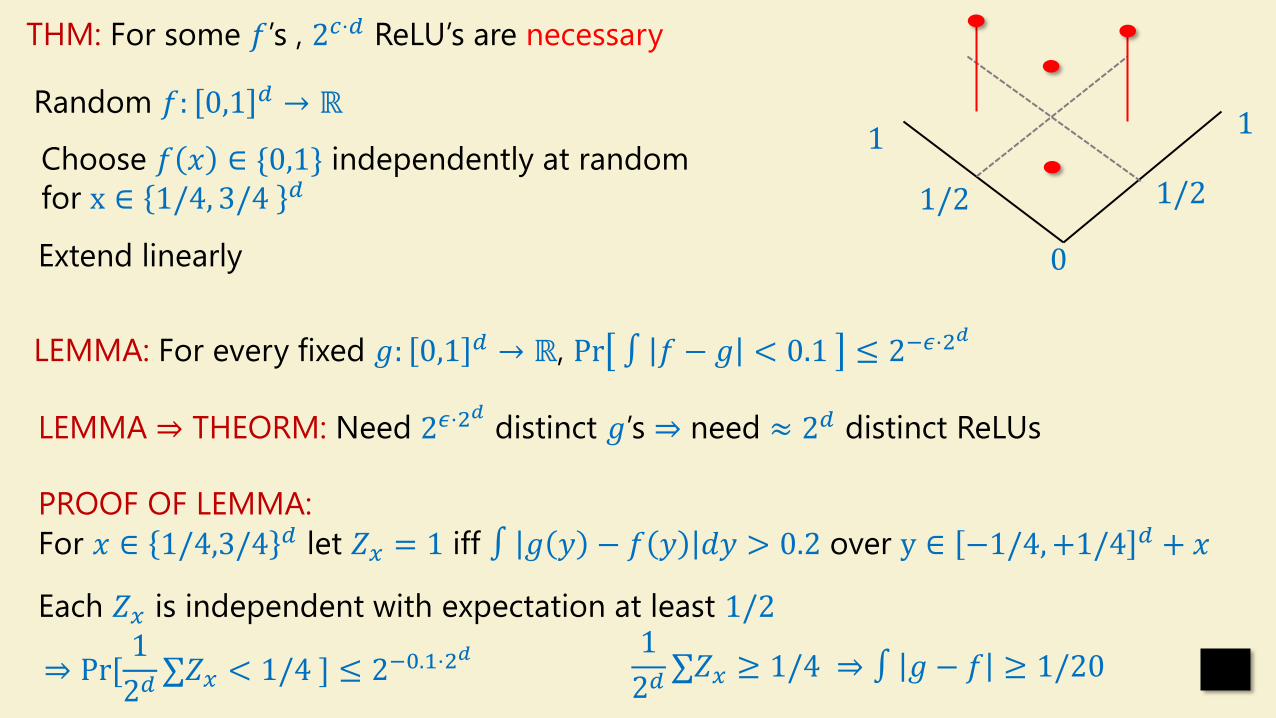
THM: For some 𝑓’s , 2𝑐⋅𝑑 ReLU’s are necessary
0
1 1
1/21/2
Random 𝑓: 0,1 𝑑 → ℝ
Choose 𝑓 𝑥 ∈ {0,1} independently at random
for x ∈ 1/4, 3/4 𝑑
Extend linearly
LEMMA: For every fixed 𝑔: 0,1 𝑑 → ℝ, Pr ∫ 𝑓 − 𝑔 < 0.1 ≤ 2−𝜖⋅2𝑑
LEMMA ⇒ THEORM: Need 2𝜖⋅2𝑑
distinct 𝑔’s ⇒ need ≈ 2𝑑 distinct ReLUs
PROOF OF LEMMA:
For 𝑥 ∈ 1/4,3/4 𝑑 let 𝑍𝑥 = 1 iff ∫ 𝑔 𝑦 − 𝑓 𝑦 𝑑𝑦 > 0.2 over y ∈ −1/4,+1/4 𝑑 + 𝑥
Each 𝑍𝑥 is independent with expectation at least 1/2
⇒ Pr[1
2𝑑σ𝑍𝑥 < 1/4 ] ≤ 2−0.1⋅2
𝑑 1
2𝑑σ𝑍𝑥 ≥ 1/4 ⇒ ∫ 𝑔 − 𝑓 ≥ 1/20
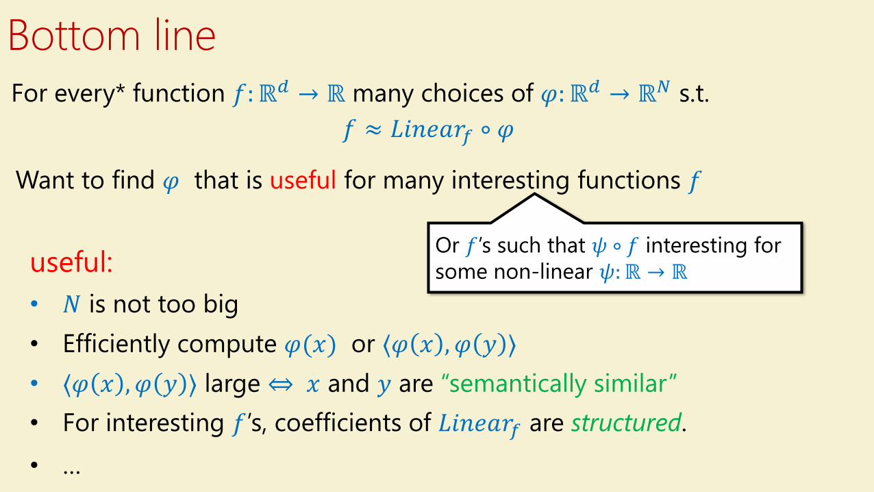
Bottom line
For every* function 𝑓:ℝ𝑑 → ℝ many choices of 𝜑:ℝ𝑑 → ℝ𝑁 s.t.
𝑓 ≈ 𝐿𝑖𝑛𝑒𝑎𝑟𝑓 ∘ 𝜑
Want to find 𝜑 that is useful for many interesting functions 𝑓
useful:
• 𝑁 is not too big
• Efficiently compute 𝜑(𝑥) or ⟨𝜑 𝑥 , 𝜑 𝑦 ⟩
• ⟨𝜑 𝑥 , 𝜑 𝑦 ⟩ large ⇔ 𝑥 and 𝑦 are “semantically similar”
• For interesting 𝑓’s, coefficients of 𝐿𝑖𝑛𝑒𝑎𝑟𝑓 are structured.
• …
Or 𝑓’s such that 𝜓 ∘ 𝑓 interesting for
some non-linear 𝜓:ℝ → ℝ

Part IV: Kernels

Neural Net
𝜑𝑥 𝐿
Kernel
𝜑𝑥 𝐿
Definitely NN Definitely Kernel
𝜑 hand-
crafted
before 1990s
𝜑 trained
end-to-end
for task at
hand
𝜑 pretrained
with same
data
𝜑 pretrained
on different
data
𝜑 pretrained
on synthetic
data
𝜑 hand-
crafted based
on neural
architectures
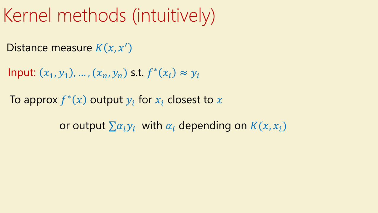
Kernel methods (intuitively)
Distance measure 𝐾 𝑥, 𝑥′
Input: 𝑥1, 𝑦1 , … , (𝑥𝑛, 𝑦𝑛) s.t. 𝑓∗ 𝑥𝑖 ≈ 𝑦𝑖
To approx 𝑓∗ 𝑥 output 𝑦𝑖 for 𝑥𝑖 closest to 𝑥
or output σ𝛼𝑖𝑦𝑖 with 𝛼𝑖 depending on 𝐾(𝑥, 𝑥𝑖)
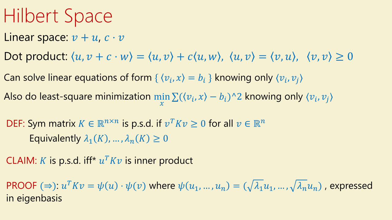
Hilbert SpaceLinear space: 𝑣 + 𝑢, 𝑐 ⋅ 𝑣
Dot product: 𝑢, 𝑣 + 𝑐 ⋅ 𝑤 = 𝑢, 𝑣 + 𝑐 𝑢,𝑤 , 𝑢, 𝑣 = 𝑣, 𝑢 , 𝑣, 𝑣 ≥ 0
Can solve linear equations of form { 𝑣𝑖 , 𝑥 = 𝑏𝑖 } knowing only ⟨𝑣𝑖 , 𝑣𝑗⟩
Also do least-square minimization min𝑥
σ( 𝑣𝑖 , 𝑥 − 𝑏𝑖)^2 knowing only ⟨𝑣𝑖 , 𝑣𝑗⟩
DEF: Sym matrix 𝐾 ∈ ℝ𝑛×𝑛 is p.s.d. if 𝑣𝑇𝐾𝑣 ≥ 0 for all 𝑣 ∈ ℝ𝑛
Equivalently 𝜆1 𝐾 ,… , 𝜆𝑛 𝐾 ≥ 0
CLAIM: 𝐾 is p.s.d. iff* 𝑢𝑇𝐾𝑣 is inner product
PROOF (⇒): 𝑢𝑇𝐾𝑣 = 𝜓 𝑢 ⋅ 𝜓(𝑣) where 𝜓 𝑢1, … , 𝑢𝑛 = ( 𝜆1𝑢1, … , 𝜆𝑛𝑢𝑛) , expressed
in eigenbasis
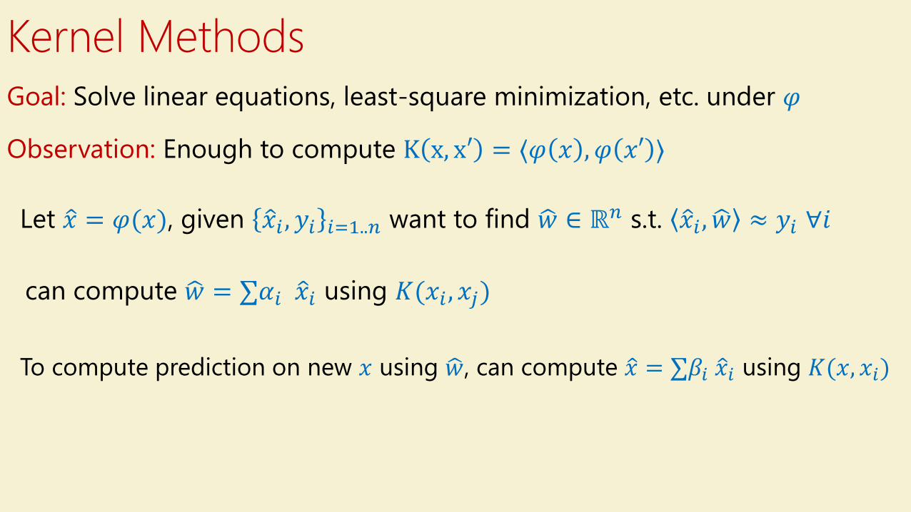
Kernel MethodsGoal: Solve linear equations, least-square minimization, etc. under 𝜑
Observation: Enough to compute K x, x′ = ⟨𝜑 𝑥 , 𝜑 𝑥′ ⟩
Let ො𝑥 = 𝜑(𝑥), given ො𝑥𝑖 , 𝑦𝑖 𝑖=1..𝑛 want to find ෝ𝑤 ∈ ℝ𝑛 s.t. ො𝑥𝑖 , ෝ𝑤 ≈ 𝑦𝑖 ∀𝑖
can compute ෝ𝑤 = σ𝛼𝑖 ො𝑥𝑖 using 𝐾(𝑥𝑖 , 𝑥𝑗)
To compute prediction on new 𝑥 using ෝ𝑤, can compute ො𝑥 = σ𝛽𝑖 ො𝑥𝑖 using 𝐾(𝑥, 𝑥𝑖)


