
Copyright © 2010 Pearson Education, Inc. 22-1
Chapter Twenty-Two
Structural Equation Modeling and Path Analysis

Copyright © 2010 Pearson Education, Inc. 22-2
Chapter Outline
1) Objectives
2) Overview
3) Basic Concepts in SEM
i. Theory, Model and Path Diagram
ii. Exogenous versus Endogenous Constructs
iii. Dependence and Correlational Relationships
iv. Model Fit
Model Identification
4) Statistics Associated with SEM

Copyright © 2010 Pearson Education, Inc. 22-3
Chapter Outline
5) Conducting SEM6) Define the Individual Constructs7) Specify The Measurement Model
i. Sample Size Requirements8) Assess Measurement Model Reliability and Validity
i. Assess Measurement Model Fita. chi-square (χ2)
b. Absolute Fit Indices: Goodness-of-Fitc. Absolute Fit Indices: Badness-of-Fitd. Incremental Fit Indicese. Parsimony Fit Indices

Copyright © 2010 Pearson Education, Inc. 22-4
Chapter Outline
ii. Measurement Model Reliability and Validity
a. Reliability
b. Discriminant Validity
iii. Lack of Validity: Diagnosing Problems9) Specify the Structural Model 10) Assess Structural Model Validity i. Assessing Fit
ii. Comparison with Competing Models
iii. Testing Hypothesized Relationships
iv. Structural Model Diagnostics

Copyright © 2010 Pearson Education, Inc. 22-5
Chapter Outline
11) Draw Conclusions and Make Recommendations
12)Higher-Order Confirmatory Factor Analysis13)Relationship of SEM to Other Multivariate
Technique14)Application of SEM: First-Order Factor Model15)Application of SEM: Second-Order Factor Model16)Path Analysis17)Statistical Software

Copyright © 2010 Pearson Education, Inc. 22-6
Structural equation modeling (SEM), a procedure for estimating a series of dependence relationships among a set of concepts or constructs represented by multiple measured variables and incorporated into an integrated model.
Structural Equation Modeling (SEM)

Copyright © 2010 Pearson Education, Inc. 22-7
1. Representation of constructs as unobservable or latent factors in dependence relationships.
2. Estimation of multiple and interrelated dependence relationships incorporated in an integrated model.
3. Incorporation of measurement error in an explicit manner. SEM can explicitly account for less than perfect reliability of the observed variables, providing analyses of attenuation and estimation bias due to measurement error.
4. Explanation of the covariance among the observed variables.
Structural Equation Modeling: Distinctive Aspects

Copyright © 2010 Pearson Education, Inc. 22-8
Absolute fit indices These indices measure the overall goodness-of-fit or badness-of-fit for both the measurement and structural models. Average variance extracted A measure used to assess convergent and discriminant validity, which is defined as the variance in the indicators or observed variables that is explained by the latent construct.Chi-square difference statistic ( Δχ2) A statistic used to compare two competing, nested SEM models. It is calculated as the difference between the models’ chi-square value. Its degrees of freedom equal the difference in the models’ degrees of freedom.Communality Communality is the variance of a measured variable that is explained by its construct.
Statistics Associated with SEM

Copyright © 2010 Pearson Education, Inc. 22-9
Composite reliability (CR) It is defined as the total amount of true score variance in relation to the total score variance. Confirmatory factor analysis (CFA) A technique used to estimate the measurement model. It seeks to confirm if the number of factors (or constructs) and the loadings of observed (indicator) variables on them conform to what is expected on the basis of theory. Construct In SEM, a construct is a latent or unobservable concept that can be defined conceptually but that cannot be measured directly or without error. Also called a factor, a construct is measured by multiple indicators or observed variables.
Statistics Associated with SEM

Copyright © 2010 Pearson Education, Inc. 22-10
Endogenous constructs An endogenous construct is the latent, multi-item equivalent of a dependent variable. It is determined by constructs or variables within the model and, thus, it is dependent on other constructs.Estimated covariance matrix Denoted by Σk , it consists of the predicted covariances between all observed variables based on equations estimated in SEM.Exogenous construct An exogenous construct is the latent, multi-item equivalent of an independent variable in traditional multivariate analysis. An exogenous construct is determined by factors outside of the model and it cannot be explained by any other construct or variable in the model.
Statistics Associated with SEM

Copyright © 2010 Pearson Education, Inc. 22-11
First-order factor model Covariances between observed variables are explained with a single latent factor or construct layer.Incremental fit indices These measures assess how well a model specified by the researcher fits relative to some alternative baseline model. Typically, the baseline model is a null model in which all observed variables are unrelated to each other.Measurement error It is the degree to which the observed variables do not describe the latent constructs of interest in SEM.
Statistics Associated with SEM

Copyright © 2010 Pearson Education, Inc. 22-12
Measurement model The first of two models estimated in SEM. It represents the theory that specifies the observed variables for each construct and permits the assessment of construct validity.Modification index An index calculated for each possible relationship that is not freely estimated but is fixed. The index shows the improvement in the overall model χ2 if that path was freely estimated.Nested model A model is nested within another model if it has the same number of constructs and variables and can be derived from the other model by altering relationships, as by adding or deleting relationships.
Statistics Associated with SEM
Copyright © 2010 Pearson Education, Inc. 22-13
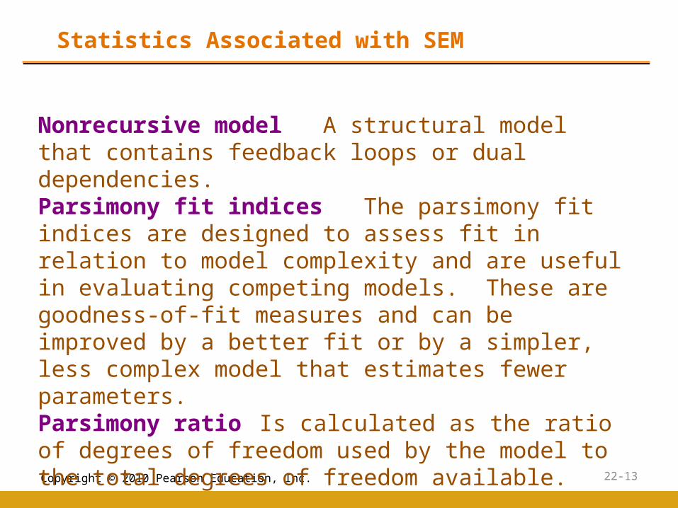
Nonrecursive model A structural model that contains feedback loops or dual dependencies.Parsimony fit indices The parsimony fit indices are designed to assess fit in relation to model complexity and are useful in evaluating competing models. These are goodness-of-fit measures and can be improved by a better fit or by a simpler, less complex model that estimates fewer parameters. Parsimony ratio Is calculated as the ratio of degrees of freedom used by the model to the total degrees of freedom available.
Statistics Associated with SEM

Copyright © 2010 Pearson Education, Inc. 22-14
Path analysis A special case of SEM with only single indicators for each of the variables in the causal model. In other words, path analysis is SEM with a structural model, but no measurement model.Path diagram A graphical representation of a model showing the complete set of relationships amongst the constructs. Dependence relationships are portrayed by straight arrows and correlational relationships by curved arrows.Residuals In SEM, the residuals are the differences between the observed and estimated covariance matrices.Recursive model A structural model that does not contain any feedback loops or dual dependencies.
Statistics Associated with SEM

Copyright © 2010 Pearson Education, Inc. 22-15
Sample covariance matrix Denoted by S, it consists of the variances and covariances for the observed variables.Second-order factor model There are two levels or layers. A second-order latent construct causes multiple first-order latent constructs, which in turn cause the observed variables. Thus, the first-order constructs now act as indicators or observed variables for the second order factor.Squared multiple correlations Similar to communality, these values denote the extent to which an observed variable’s variance is explained by a latent construct or factor.
Statistics Associated with SEM
Copyright © 2010 Pearson Education, Inc. 22-16
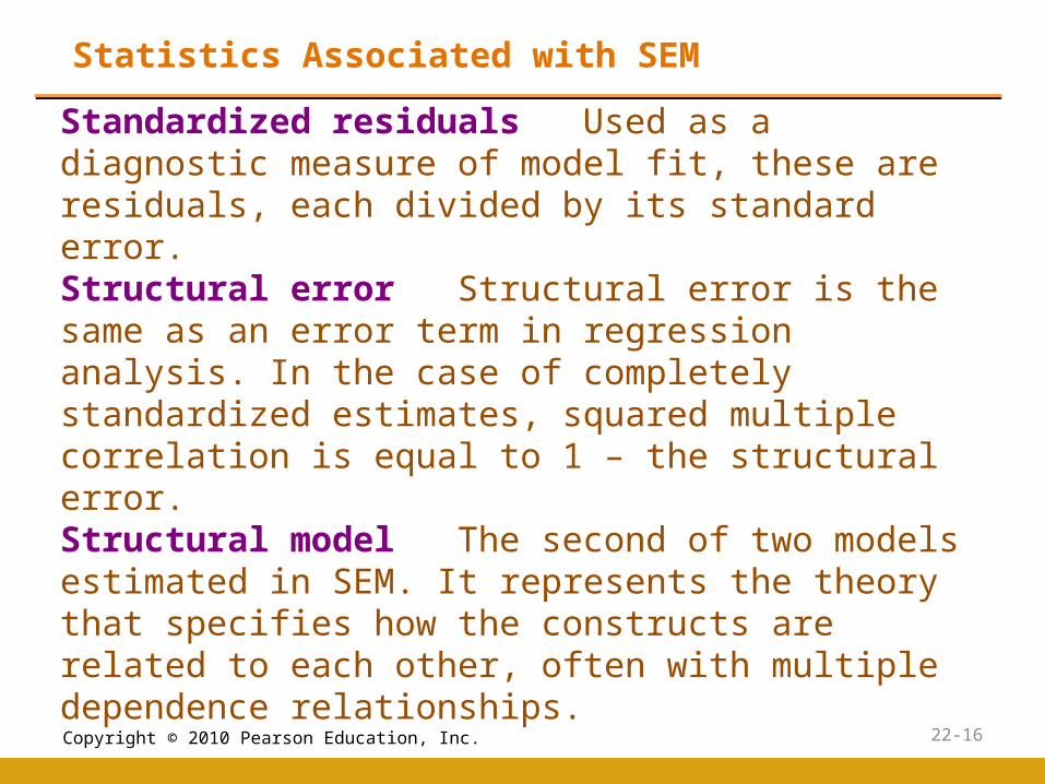
Standardized residuals Used as a diagnostic measure of model fit, these are residuals, each divided by its standard error.Structural error Structural error is the same as an error term in regression analysis. In the case of completely standardized estimates, squared multiple correlation is equal to 1 – the structural error. Structural model The second of two models estimated in SEM. It represents the theory that specifies how the constructs are related to each other, often with multiple dependence relationships.
Statistics Associated with SEM
Copyright © 2010 Pearson Education, Inc. 22-17
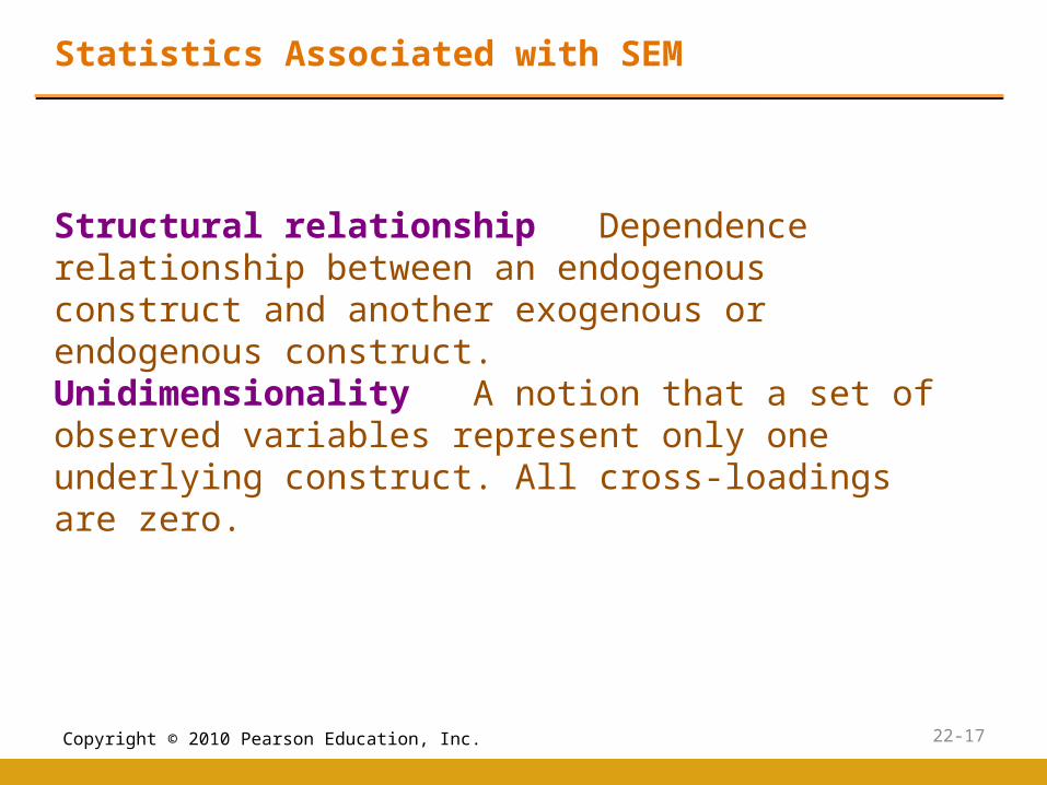
Structural relationship Dependence relationship between an endogenous construct and another exogenous or endogenous construct.Unidimensionality A notion that a set of observed variables represent only one underlying construct. All cross-loadings are zero.
Statistics Associated with SEM

Copyright © 2010 Pearson Education, Inc. 22-18
Exogenous and Endogenous Constructs
Exogenous constructs are the latent, multi-item equivalent of independent variables. They use a variate (linear combination) of measures to represent the construct, which acts as an independent variable in the model.Multiple measured variables (X) represent the exogenous
constructs (ξ).
Endogenous constructs are the latent, multi-item equivalent to dependent variables. These constructs are theoretically determined by factors within the model.Multiple measured variables (Y) represent the endogenous
constructs (η).

Copyright © 2010 Pearson Education, Inc. 22-19
Models can be represented visually with a path diagram.
Dependence relationships are represented with single-headed straight arrows.
Correlational (covariance) relationships are represented with two-headed curved arrows.
SEM Models

Copyright © 2010 Pearson Education, Inc. 22-20
(a) Dependence Relationship
ExogenousConstruct: C1
EndogenousConstruct: C2
X1 X2 X3Y1 Y2 Y3
Dependence and Correlational Relationships in SEM
Fig. 22.1Fig. 22.1Fig. 22.1

Copyright © 2010 Pearson Education, Inc. 22-21
ExogenousConstruct: C1
ExogenousConstruct: C2
X1 X2 X3 X4X5 X6
Dependence and Correlational Relationships in SEM
Fig. 22.1 Cont.

Copyright © 2010 Pearson Education, Inc. 22-22
Conducting SEM
Steps in SEM
Step 1: Define the Individual Constructs Step 2: Specify the Measurement ModelStep 3: Assess Measurement Model Reliability and
ValidityStep 4: Specify the Structural ModelStep 5: Assess Structural Model ValidityStep 6: Draw Conclusions and Make
Recommendations

Copyright © 2010 Pearson Education, Inc. 22-23
The Process for Structural Equation Modeling
Define the Individual Constructs
Develop and Specify the Measurement Model
Assess Measurement Model Reliability and Validity
Specify the Structural Model
Assess Structural Model Validity
Draw Conclusions and Make Recommendations
Measurement ModelValid?
Refine Measures andDesign a New Study
YES
NO
Structural Model Valid?
YES
Refine Model and Test with New
Data
No
Fig. 22.2

Copyright © 2010 Pearson Education, Inc. 22-24
Path Diagram of a Simple Measurement Model
C1
ξ1
C2
ξ2
X1 X2 X3 X4 X5 X6
λx1,1 λ
X2,1
λX4,2
λX5,2
λx6,2
Φ21
δ4 δ5 δ6 δ1 δ2 δ3
λх3,1
Fig. 22.3

Copyright © 2010 Pearson Education, Inc. 22-25
In Figure 22.3, ξ1 represents the latent construct C1 , ξ2 represents the latent construct C2, x1 - x6 represent the measured variables, λx1,1 - λχ6,2 represent the relationships between
the latent constructs and the respective measured items (i.e; factor loadings), and
δ1 - δ6 represent the errors.
A Simple Measurement Model

Copyright © 2010 Pearson Education, Inc. 22-26
1. Absolute fit measures overall goodness- or badness-of-fit for both the structural and measurement models. This type of measure does not make any comparison to a specified null model (incremental fit measure) or adjusts for the number of parameters in the estimated model (parsimonious fit measure).
2. Incremental fit measures goodness-of-fit that compares the current model to a specified “null” (independence) model to determine the degree of improvement over the null model.
3. Parsimonious fit measures goodness-of-fit representing the degree of model fit per estimated coefficient. This measure attempts to correct for any “overfitting” of the model and evaluates the parsimony of the model compared to the goodness-of-fit.
Types of Fit Measures

Copyright © 2010 Pearson Education, Inc. 22-27
A Classification of Fit Measures
Absolute Fit Incremental Parsimony Indices Fit Indices Fit Indices
Goodness-of-Fit Badness-of-Fit Goodness-of-Fit
• NFI
• NNFI
• CFI
• TLI
• RNI
Goodness-of-Fit
PGFI
PNFI
• GFI
• AGFI
• x2
• RMSR
• SRMR
• RMSEA
Fit MeasuresFig. 22.4

Copyright © 2010 Pearson Education, Inc. 22-28
Assessing Model Fit: Chi-square
))(1( kSn
kppdf )]1)([(2
1

Copyright © 2010 Pearson Education, Inc. 22-29
Multiple fit indices should be used to assess a model’s goodness of fit. They should include:
• The χ2 value and the associated df
• Two absolute fit indices (GFI, AGFI, RMSEA, or SRMR)
• One goodness-of-fit index (GFI, AGFI)
• One badness-of-fit index (RMSR, SRMR, RMSEA)
• One incremental fit index (CFI, TLI, NFI, NNFI, RNI)
• One parsimony fit index for models of different complexities (PGFI, PNFI)
Assessing Model Fit: Fit Indexes

Copyright © 2010 Pearson Education, Inc. 22-30
Where
CR = Composite reliability
λ = completely standardized factor loading
δ = Error variance
p = number of indicators or observed variables
CR = (∑ λi )2
(∑λi)2 + (∑δi)
p
i=1
i=1 i=1
p p
Composite Reliability (CR)

Copyright © 2010 Pearson Education, Inc. 22-31
p 2 Σ λί
i=1 AVE = p 2 p
Σ λί + Σ δi
i=1 i=1
Where
AVE = Average variance extracted
λ = Completely Standardized factor loading
δ = Error variance
p = number of indicators or observed variables
Average Variance Extracted (AVE)

Copyright © 2010 Pearson Education, Inc. 22-32
Path Diagram of a Simple Structural Model
Construct 1: C1
ξ1
Construct 2:C2 η1
X1 X2 X3 Y1 Y2 Y3
γ1,1
λx1,1
λx2,1
λy1,1
λy2,1
δ1 δ2δ3
ε1 ε2 ε3
λy3,1λx3,1
Fig. 22.5

Copyright © 2010 Pearson Education, Inc. 22-33
Δχ2Δdf = χ2
df(M1) - χ2df(M2)
and
Δdf = df(M1) –df(M2)
Chi-Square Difference Test

Copyright © 2010 Pearson Education, Inc. 22-34
First-Order Model of IUIPC
COL CON AWA
X1 X2 X3 X4 X5 X6X7 X8 X9 X10
Φ2,1 Ф3,2
Ф3,1
Fig. 22.6

Copyright © 2010 Pearson Education, Inc. 22-35
Second-Order Model of IUIPC
IUIPC Layer 2
COL CON AWA
Layer 1
X1 X3 X4X2 X5 X6 X7 X10X8 X9
X1,1 X2,1
X3,1
Legend:First-Order Factors: COL = Collection CON = Control AWA = Awareness
Second-Order Factor : IUIPC = Internet Users Information Privacy Concerns
Fig. 22.7

Copyright © 2010 Pearson Education, Inc. 22-36
Measurement Model for TAM
PU PE INT
PU1 PU2 PU3 PE1 PE2 PE3 INT1 INT2 INT3
Φ2,1 Ф3,2
Ф3,1Fig. 22.8

Copyright © 2010 Pearson Education, Inc. 22-37
Structural Model for TAM
Perceived Usefulness
PU
Perceived Ease Of Use
PE
Intentionto Use
INT
0.46
0.28
0.40
0.60
Fig. 22.9

Copyright © 2010 Pearson Education, Inc. 22-38
ME SD Correlations Matrix
1 2 3 4 5 6 7 8 9
1. PU1 3.58 1.37 1 2. PU2 3.58 1.37 .900** 1 3. PU3 3.58 1.36 .886** .941** 1 4. PE1 4.70 1.35 .357** .403** .392** 1 5. PE2 4.76 1.34 .350** .374** .393** .845** 1 6. PE3 4.79 1.32 .340** .356** .348** .846** .926** 1 7. INT1 3.72 2.10 .520** .545** .532** .442** .419** .425** 1 8. INT2 3.84 2.12 .513** .537** .540** .456** .433** .432** .958** 1 9. INT3 3.68 2.08 .534** .557** .559** .461** .448** .437** .959** .950** 1
Notes: ME = means; SD = standard deviations; *p<0.05, **p<0.01, ***p<0.001 (two-tailed).
TAM: Means, Standard Deviations, and CorrelationsTable 22.1Table 22.1

Copyright © 2010 Pearson Education, Inc. 22-39
Constructs Items Item Loadings Item Errors CR AVE
PU 0.97 0.91 PU1 0.92*** 0.15*** PU2 0.98*** 0.05*** PU3 0.96*** 0.07***
PE 0.95 0.87 PE1 0.88*** 0.23*** PE2 0.96*** 0.07*** PE3 0.96*** 0.08***
INT 0.98 0.95 INT2 0.98*** 0.03*** INT2 0.97*** 0.05*** INT3 0.98*** 0.05***
Notes: CR = composite reliability; AVE = average variance extracted. *p<0.05, **p<0.01, ***p<0.001 (two-tailed).
TAM: Results of Measurement Model
Table 22.2

Copyright © 2010 Pearson Education, Inc. 22-40
x1 x2x3
x4X5
X6 X7X8
X9 x10 X11 x12 x13 x14 X16X15 X17 x18 x19 x20 x21 x22 x23x28
x24 X29
TANG ξ1 REL ξ2 RESP ξ3 ASS4 ξ4 EMP ξ5 ATT ξ6 SAT ξ7 PAT ξ8
δ1 δ2 δ3 δ4 δ5 δ6 δ7 δ8 δ9 δ10 δ11 δ12 δ13 δ14 δ15 δ16 δ17 δ18 δ19 δ20 δ21 δ22 δ23 δ24 δ25 δ26 δ27 δ28 δ29 δ30
Banking Application: Measurement Model
x25 x26 x27 x30
Fig. 22.10

Copyright © 2010 Pearson Education, Inc. 22-41
Service Quality
TANG
REL
RESP
ASSU
Patronage Intention
Service Attitude
Service Satisfaction
EMP
TANG = tangibility; REL= reliability; RESP = responsiveness; ASSU = assurance; EMP = empathy
Banking Application: Structure Model
Fig. 22.11

Copyright © 2010 Pearson Education, Inc. 22-42
When it comes to…. My Perception of My
Bank’s Service.
TANG1: Modern equipments
TANG2: Visual appeal of physical facilities
TANG3: Neat, professional appearance of employees
TANG4: Visual appeal of materials associated with the service
REL1: Keeping a promise by a certain time
REL2: Performing service right the first time
REL3: Providing service at the promised time
REL4: Telling customers the exact time the service will be performed
Loadings Measurement Error
0.71 0.49
0.80 0.36
0.76 0.42
0.72 0.48
0.79 0.37
0.83 0.31
0.91 0.18
0.81 0.34
Psychometric Properties of Measurement ModelTable 22.3

Copyright © 2010 Pearson Education, Inc. 22-43
When it comes to…. My Perception of My
Bank’s Service.
RESP1: Keeping a promise by a certain time
RESP2: Willingness to always help customers
RESP3: Responding to customer requests despite being busy
ASSU1: Employees instilling confidence in customers
ASSU2: Customers’ safety feelings in transactions (e.g. physical, financial, emotional, etc.)
ASSU3: Consistent courtesy to customers
ASSU4: Employees’ knowledge to answer customer questions
Loadings Measurement Error
0.73 0.47
0.89 0.21
0.81 0.35
0.81 0.35
0.71 0.49
0.80 0.36
0.86 0.26
Psychometric Properties of Measurement Model
Table 22.3 Cont.
Copyright © 2010 Pearson Education, Inc. 22-44
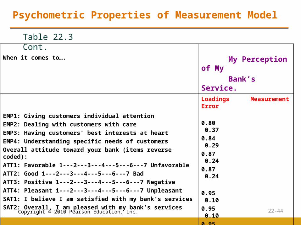
When it comes to…. My Perception of My
Bank’s Service.
EMP1: Giving customers individual attention
EMP2: Dealing with customers with care
EMP3: Having customers’ best interests at heart
EMP4: Understanding specific needs of customers
Overall attitude toward your bank (items reverse coded):
ATT1: Favorable 1---2---3---4---5---6---7 Unfavorable
ATT2: Good 1---2---3---4---5---6---7 Bad
ATT3: Positive 1---2---3---4---5---6---7 Negative
ATT4: Pleasant 1---2---3---4---5---6---7 Unpleasant
SAT1: I believe I am satisfied with my bank’s services
SAT2: Overall, I am pleased with my bank’s services
Loadings Measurement Error
0.80 0.37
0.84 0.29
0.87 0.24
0.87 0.24
0.95 0.10
0.95 0.10
0.95 0.10
0.95 0.10
0.93 0.14
0.93 0.14
Psychometric Properties of Measurement Model
Table 22.3 Cont.

Copyright © 2010 Pearson Education, Inc. 22-45
When it comes to…. My Perception of My
Bank’s Service.
SAT3: Using services from my bank is usually a satisfying
experience
SAT4: My feelings toward my bank’s services can best be
characterized as
PAT1: The next time my friend needs the services of a bank
I will recommend my bank
PAT2: I have no regrets of having patronized my bank in the past
PAT3: I will continue to patronize the services of my bank in the
future
Loadings Measurement Error
0.88 0.23
0.92 0.15
0.88 0.22
0.89 0.20
0.88 0.22
Table 22.3 Cont.
Psychometric Properties of Measurement Model

Copyright © 2010 Pearson Education, Inc. 22-46
----------------------------------------------Degrees of Freedom = 377
Minimum Fit Function Chi-Square = 767.77 (P = 0.0)
Chi-Square for Independence Model with 435 Degrees of Freedom = 7780.15
Root Mean Square Error of Approximation (RMSEA) = 0.064
Standardized RMR = 0.041
Normed Fit Index (NFI) = 0.90Non-Normed Fit Index (NNFI) = 0.94Comparative Fit Index (CFI) = 0.95
----------------------------------------------
Table 22.4
Goodness of Fit Statistics Measurement Model

Copyright © 2010 Pearson Education, Inc. 22-47
Measurement Model: Construct Reliability, Average Variance Extracted & Correlation Matrix
Construct ConstructReliability
AverageVarianceExtracted
Correlation Matrix1 2 3 4 5 6 7 8
1. TANG
0.84
0.56 0.75
2. REL
0.90 0.70 0.77 0.84
3. RESP
0.85 0.66 0.65 0.76 0.81
4. ASSU
0.87 0.63 0.73 0.80 0.92 0.80
5. EMP
0.91 0.71 0.69 0.75 0.85 0.90 0.85
6. ATT
0.97 0.90 0.42 0.46 0.52 0.54 0.58 0.95
7. SAT
0.85 0.83 0.53 0.56 0.66 0.67 0.69 0.72 0.91
8. PAT
0.92 0.78 0.50 0.55 0.57 0.62 0.62 0.66 0.89 0.89
TANG = tangibles; REL = reliability; RESP = responsiveness; ASSU = assurance; EMP = empathy; ATT = attitude; SAT = satisfaction; PAT = patronage. Value on the diagonal of the correlation matrix is the square root of AVE.
Table 22.5

Copyright © 2010 Pearson Education, Inc. 22-48
---------------------------------------------------------------------------------
Degrees of Freedom = 396Minimum Fit Function Chi-Square = 817.16 (P = 0.0)
Chi-Square for Independence Model with 435 Degrees of Freedom = 7780.15Root Mean Square Error of Approximation (RMSEA) = 0.065
Standardized RMR = 0.096
Normed Fit Index (NFI) = 0.89Non-Normed Fit Index (NNFI) = 0.94Comparative Fit Index (CFI) = 0.94
---------------------------------------------------------------------------------------------------------------
Table 22.6
Goodness of Fit Statistics (Structural Model)

Copyright © 2010 Pearson Education, Inc. 22-49
Banking Application: Structural Coefficients
Dimensions of Service Quality
Second Order T-values Loading Estimates
TANG 0.82 fixed to 1
REL 0.85 13.15
RESP 0.93 13.37
ASSU 0.98 16.45
EMP 0.93 15.18
Table 22.7Table 22.7

Copyright © 2010 Pearson Education, Inc. 22-50
SQATT 0.60 10.25
SQSAT 0.45 8.25
ATTSAT 0.47 8.91
ATTPAT 0.03 0.48
SATPAT 0.88 13.75
Consequences of
Service Quality
StructuralCoefficient Estimates
T-Values
Table 22.7 Cont.
Banking Application: Structural Coefficients

Copyright © 2010 Pearson Education, Inc. 22-51
Path analysis A special case of SEM with only single indicators for each of the variables in the causal model. In other words, path analysis is SEM with a structural model, but no measurement model.
Path Analysis

Copyright © 2010 Pearson Education, Inc. 22-52
Diagram for Path Analysis
B
C
A
X1
Attitude
X2
Emotion
Y1
PurchaseIntention
Fig. 22.12
Copyright © 2010 Pearson Education, Inc. 22-53
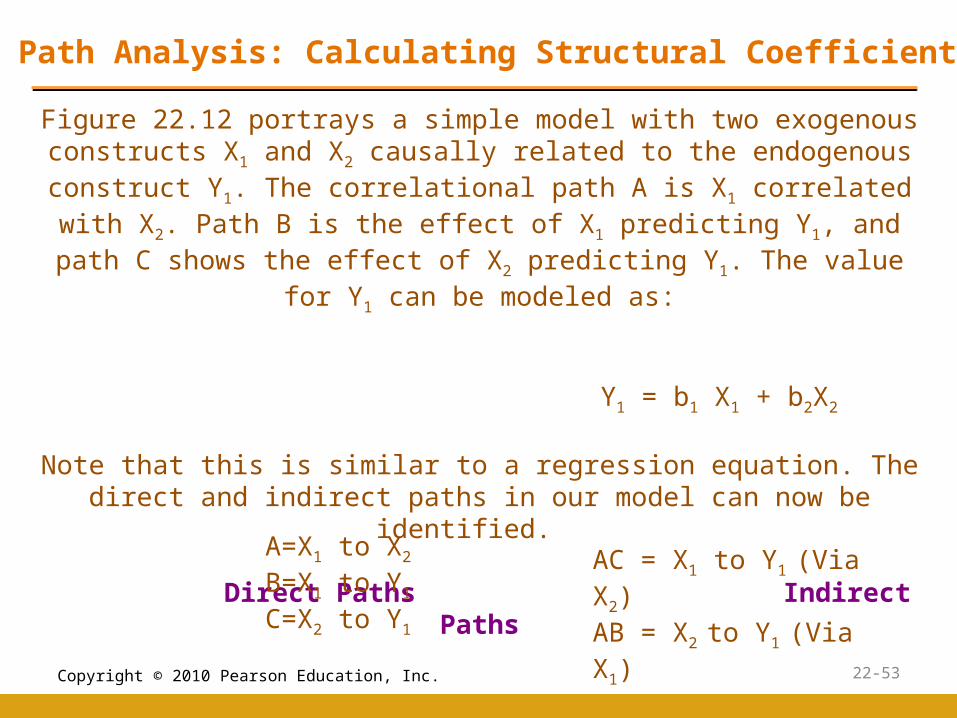
Figure 22.12 portrays a simple model with two exogenous constructs X1 and X2 causally related to the endogenous construct Y1. The correlational path A is X1 correlated with X2. Path B is the
effect of X1 predicting Y1, and path C shows the effect of X2 predicting Y1. The value for Y1 can be modeled as:
Y1 = b1 X1 + b2X2
Note that this is similar to a regression equation. The direct and indirect paths in our model can now be identified.
Direct Paths Indirect PathsA=X1 to X2
B=X1 to Y1
C=X2 to Y1
AC = X1 to Y1 (Via X2)AB = X2 to Y1 (Via X1)
Path Analysis: Calculating Structural Coefficients

Copyright © 2010 Pearson Education, Inc. 22-54
Path Analysis: Calculating Structural Coefficients
The unique correlations among the three constructs can be shown to be composed of direct and indirect paths as follows:
Corrx1, x2 = A
Corrx1, y1 = B + ACCorrx2, y1 = C + AB
The correlation of X1 and X2 is simply equal to A. The Correlationof X1 and Y1 ( Corrx1,y1 ) can be represented by two paths:B and AC. B represents the direct path from X1 to Y1. AC is a compound path that follows the curved arrow from X1 to X2 and then to Y1. Similarly, the correlation of X2 and Y1 can be shown to consist of two causal paths: C and AB.

Copyright © 2010 Pearson Education, Inc. 22-55
Bivariate Correlations
X1 X2 Y1
X1 1.0
X2 .40 1.0
Y1 .50 .60 1.0
Path Analysis

Copyright © 2010 Pearson Education, Inc. 22-56
Correlations as Compound Paths
Corr X1, X2 = A
Corr X1 ,Y1 = B+AC
Corr X2 ,Y1 = C+AB
Path Analysis

Copyright © 2010 Pearson Education, Inc. 22-57
.40 = A
.50 = B+AC
.60 = C+AB
Substituting A = .40.50 = B+.40C.60 = C+.40B
Solving for B and CB = .310C = .476
Path Analysis: Calculating Structural Coefficients

Copyright © 2010 Pearson Education, Inc. 22-58
Statistical Software
•LISREL, LInear Structural RELations
•AMOS, Analysis of Moment Structures, is an added module to SPSS
•CALIS is offered by SAS
•EQS, an abbreviation for equations
•Mplus is another software
Selection of a specific computer program should be based on availability and user’s preference.

Copyright © 2010 Pearson Education, Inc. 22-59

Copyright © 2010 Pearson Education, Inc. 22-60
All rights reserved. No part of this publication may be reproduced, stored in a retrieval system, or transmitted, in
any form or by any means, electronic, mechanical, photocopying, recording, or otherwise, without the prior written permission of the publisher. Printed in the United
States of America.
Copyright © 2010 Pearson Education, Inc.


