
Coordinated and controlled mobility of multiple sinksfor maximizing the lifetime of wireless sensor networks
Stefano Basagni • Alessio Carosi • Chiara Petrioli •
Cynthia A. Phillips
Published online: 8 January 2011
� Springer Science+Business Media, LLC 2011
Abstract We define scalable models and distributed
heuristics for the concurrent and coordinated movement of
multiple sinks in a wireless sensor network, a case that
presents significant challenges compared to the widely
investigated case of a single mobile sink. Our objective is
that of maximizing the network lifetime defined as the time
from the start of network operations till the failure of the
first node. We contribute to this problem providing three
new results. We first define a linear program (LP) whose
solution provides a provable upper bound on the maximum
lifetime possible for any given number of sinks. We then
develop a centralized heuristic that runs in polynomial time
given the solution to the LP. We also define a deployable
distributed heuristic for coordinating the motion of multi-
ple sinks through the network. We demonstrate the per-
formance of the proposed heuristics via ns2-based
simulations. The observed results show that our distributed
heuristic achieves network lifetimes that are remarkably
close to the optimum ones, resulting also in significant
improvements over the cases of deploying the sinks
statically, of random sink mobility and of heuristics pre-
viously proposed for restricted sink movements.
Keywords Wireless sensor networks �Mobility management � Sink mobility �Multi-sink mobile sensor networks
1 Introduction
One of the most promising recent research directions for
performance improvement in wireless sensor networks
(WSNs) [1] is exploiting the mobility of some of the net-
work components. This mitigates the so called sink
neighborhood problem, where many nodes send packets to
a few data collection points (the sinks), funneling data
through the network and placing increasing burdens on
sensors close to the sinks. If the sinks are statically
deployed, sensors near the sink expend energy at a rate
much faster than sensors far from the sinks. When these
nodes have drained their batteries, the sink cannot receive
any further packets. Moving network components—
whether the sensors or the sinks—can better balance energy
depletion among the nodes, prolonging network lifetime,
i.e., the time the network is able to perform its functions.1
Devices could move independently of the network status.
S. Basagni
Department of Electrical and Computer Engineering,
Northeastern University, Boston, MA, USA
e-mail: [email protected]
A. Carosi � C. Petrioli (&)
Dipartimento di Informatica, Universita di Roma ‘‘La Sapienza’’,
Rome, Italy
e-mail: [email protected]
A. Carosi
e-mail: [email protected]
C. A. Phillips
Sandia National Laboratories, Albuquerque, NM, USA
e-mail: [email protected]
1 Definitions of network lifetime vary, and depend on applications. In
this paper we adopt the widely used definition introduced in [2] and
used in many works (see [3, 4] and references therein) where lifetime
is defined as the time until the failure (here for energy depletion) of
the first node. This definition may seem too pessimistic, and many
advocate definitions based on the failure of a certain percentage of the
nodes. However, robust, energy-efficient protocols for WSNs tend to
balance energy consumption among the nodes. So when the first node
dies, many other nodes are also about to die.
123
Wireless Netw (2011) 17:759–778
DOI 10.1007/s11276-010-0313-8

For instance, they can travel randomly through the nodes,
or in predetermined oblivious patterns (such as snaking or
in a spiral). Alternatively, the devices could choose to
move to specific locations based on key network param-
eters, such as the energy available at the nodes, energy
consumption patterns, traffic load, etc. This is called
controlled mobility.
In this paper we investigate network performance
improvement via controlled and coordinated sink mobility.
Appropriately scheduling sink movements can enable
applications where long network lifetime is critical. For
instance, structural health monitoring, as of a subway
tunnel, is naturally performed by embedding small sensors
into the structure. The sensors transmit data to small por-
table computers (sinks) which have high data rate con-
nections with the monitoring center. Moving these sinks
over time based upon evolving network conditions
remarkably prolongs sensor lifetime without seriously
impacting other metrics, as we show in this paper.
This paper provides clear evidence that controlled and
coordinated mobility of multiple sinks achieves signifi-
cantly better performance than uncontrolled movement or
static sinks. Our review of the initial research on this topic
(presented in details in the next section) found no analytical
solutions for controlled and coordinated mobility of mul-
tiple sinks. We have also found no distributed protocols for
coordinated and controlled mobility of sinks, which are
needed for realistic deployments. We begin to fill this gap
by making a threefold contribution. We provide a new
scalable mathematical model that provides a provable
upper bound on network lifetime. We give a centralized
heuristic to compute sink movement schedules. These
solutions are needed to provide provable bounds on the
best possible network performance (e.g., the best achiev-
able lifetime) as well as for benchmarking more realistic
protocols. The third contribution is a realistically deploy-
able distributed heuristic for the coordinated and controlled
movement of multiple sinks.
Our new mathematical model flexibly captures realistic
aspects of WSNs. It allows varying sensor deployment and
has several parameters to control data generation rate,
routing schemes, and energy costs for sensor tasks. The
mixed integer linear programming (MILP) model defined
for a single mobile sink [5] cannot be extended directly to
multiple sinks. The main challenge here is scaling to model
networks with hundreds of sensors or more. This is because
at any given time a suitable MILP model must choose an
active sink to receive the packets from each sensor. Natural
linear ways to propagate this choice for calculating energy
consumption yield weak linear programming (LP) relax-
ations and therefore long solve times. We achieve scala-
bility by defining an LP model that provides an upper
bound on the maximum lifetime possible for any given
number of sinks. The LP has an exponential number of
constraints, but we can compute the optimal solution effi-
ciently by iteratively generating and adding a violated
constraint and re-solving the LP a polynomial number of
times. Our solution is quite technical, but allows us to
compute an upper bound on the maximum lifetime for
WSNs that are quite realistic, e.g., made up of 400 nodes,
with 64 different positions where the sinks can sojourn
(called sink sites), and with 5 sinks concurrently roaming
throughout the network.
Starting from the output of the LP we define a new
polynomial-time centralized heuristic for finding a full
schedule for the movement of the sinks. Solutions provided
by our scalable heuristic (described in detail in Sect. 4)
obtain network lifetimes that are less than 1% below the
upper bound obtained from the LP-based relaxation.
A further contribution of this work is the definition of a
realistically deployable distributed protocol for controlling
and coordinating the motion of multiple sinks through the
network. The idea behind our protocol is to trigger the
movement of each sink depending on the expected lifetime
improvement that can be obtained by that move. Move-
ments are dictated by the nodes’ residual energy and by
energy consumption patterns. A sink moves if and only if
sojourning at a new position yields a longer (expected)
lifetime (controlled sink mobility). By gathering network
state information efficiently, sinks can make this decision
locally and share it with fellow sinks. So, sink deci-
sions take into account the decisions of others (sink
coordination).
We conclude the paper by showing the results of a
comparative performance evaluation of the proposed solu-
tions, namely, the LP-based upper bound, the centralized
heuristic, the distributed protocols for sink mobility, and
protocols where sink mobility is uncontrolled and random.
We also compare all these mobility schemes to the case
where the sinks are statically and optimally placed and
against the best performing solutions for multiple sink
mobility presented by Azad and Chockalingam [6]. The
experimental results show that our distributed heuristic
achieves network lifetimes that are remarkably close to
optimal. They were between 5.5 and 25.3% below the upper
bound in all the scenarios we considered. The improve-
ments over random sink mobility are also significant: up to
88.2%. The lifetime from our distributed algorithm can be
fourfold higher than the lifetime from optimally placed
static sinks and up to 40% higher than the lifetime from
Azad and Chockalingam’s heuristics Max-Min-RE and
MinDiff-RE [6]. These results show clearly that controlling
and coordinating the mobility of sinks remarkably prolongs
the lifetime of realistically deployable WSNs.
The rest of the paper is organized as follows. In the next
section we review previous works on the placement and
760 Wireless Netw (2011) 17:759–778
123
exploitation of mobility of multiple sinks. We give prob-
lem formulation details in Sect. 3. In Sect. 4 we describe
the LP model that provides upper bounds on the optimal
network lifetime. The scalable centralized heuristic and the
distributed heuristic are described in Sects. 5 and 6,
respectively. In Sect. 7 we present ns2-based simulations to
validate our centralized and distributed schemes and to
compare them to the upper bound, the Max-Min-RE and
MinDiff-RE centralized heuristics, static sink placement
and random mobility. Section 8 concludes the paper.
2 Related works
Improving WSN lifetime by exploiting the mobility of
multiple sinks involves determining routes for the sinks
and their sojourn times at designated sites so that the
lifetime is maximized.
Gandham et al. [7] propose the first work on multi-sink
WSNs, improving lifetime indirectly by greedily mini-
mizing nodal energy consumption. They divide time into
rounds. At the beginning of each round they solve a static
sink placement problem to reposition the sinks based on the
current energy in the network nodes. Specifically, they
centrally gather the residual energy of all nodes. Then they
solve an integer linear program (ILP) to determine new
sink locations that minimize the maximum energy expen-
ded by any node in the next round, subject to the constraint
that no node expends more than an a fraction of its current
residual energy. The ILP also determines packet trans-
mission rates for each node to its neighbors. The sensors
then route packets to outgoing edges in a round robin based
on the proportions given by the ILP. Experiments show that
this algorithm with three sinks extends lifetime consider-
ably compared to deploying one static sink. This first effort
to address deployment of multiple sinks does not consider
many important characteristics of WSNs. For instance,
although the ILP models minimize nodal energy con-
sumption in each round, this greedy approach does not
guarantee a globally optimal lifetime. Moreover, the ILP
models do not consider energy spent for route manage-
ment, which is non-negligible, and is routing dependent.
Azad and Chockalingam [6] propose three centralized
heuristics for the models and setting of [7], where s � 1
sinks can sojourn only at v � s sites on the boundary of
the network deployment region. In the first heuristic,
Top-Kmax, the authors let the residual energy of a sink site
i be the residual energy of the sensor closest to i. At the
start of each round, they place the s sinks at the s sink sites
with the highest residual energy. The second heuristic is
called Max-Min-RE because it chooses a sink configuration
where the most heavily loaded node (the one with
minimum residual energy, Min-RE) will have the maxi-
mum energy at the end of the next round. To more evenly
drain the nodes, the third heuristic (MinDiff-RE), chooses
the configuration that minimizes (Min) the difference
(Diff) between the maximum and minimum residual
energy (RE) over all nodes. The latter two solutions require
the enumeration of all possiblevs
� �sink placements, and
are therefore viable only when the number of sinks is very
limited.
Ren et al. [8] investigate the impact of multiple mobile
sinks on end-to-end packet delay and energy consumption.
They consider trade offs for optimizing both. Specifically,
deploying sinks moving in an uncontrolled way (random
way-point), they investigate the impact of sink number,
speed, sink transmission radius, and data routing on per-
formance. Single-hop collection minimizes the energy but
results in higher latencies, so that in many applications
multi-hop communication is the only viable option. The
authors conclude that the number of sinks, their speed and
the routing can be tuned to provide acceptable delays and
energy consumption, i.e., to obtain a required network
lifetime. They also observe through simulations that
(uncontrolled) sink mobility yields more balanced energy
consumption compared to static sinks. Chen and Ma, with
Yu, continue to investigate this topic in [9], where rather
than mobile sinks, they explore a three-tier architecture
where cellular phones, whose mobility is uncontrolled, act
similarly to data MULEs and carry data to a single base
station.
Recently, Chatzigiannakis et al. [10] propose three
solutions for efficient data collection via mobile sinks.
They wish to move sinks to reduce nodal energy con-
sumption, prolong network lifetime, increase delivery rate,
and decrease packet latency with respect to the case with
one sink roaming through the network. Packet routing from
the sensors to the sinks is single hop, i.e., a sensor must be
visited by a sink in order to deliver its data. The first
protocol is centralized: The deployment area is partitioned
into equally sized regions, each of which is assigned a sink
that traverses it exhaustively in a snake fashion. This
solution is particularly suitable when the network is fairly
stable and homogeneous. No actual coordination is needed
among the sinks, since each region is an independent col-
lection problem. The second protocol requires some loose
coordination of the sinks. The s sinks are initially deployed
randomly. Each moves in a random walk through the entire
network area. Each sink transmits a beacon message con-
taining its ID, its position, speed and direction. This
information is stored at the sensors that receive it for a
predefined time t. If another sink comes by within t time
from the passing of a previous sink, the new one changes
Wireless Netw (2011) 17:759–778 761
123
its direction, thus avoiding traversing an area visited
recently by some other sink. The third protocol partitions
the network into small clusters and assigns clusters to
sinks. Clusters have weights that depend on critical cluster
parameters such as the traffic load, nodal residual energy,
etc. If there are s sinks, the protocol then combines clusters
into s groups with roughly equal weight. Every sink does a
random walk through its clusters, collecting data from
nodes in its group in a single-hop fashion. Experimental
results show that the proposed protocols achieve good
performance using only up to four sinks.
3 Problem formulation
We consider networks with a small number s of mobile sinks
that collect data from a large set N of deployed resource-
constrained sensor nodes. Sinks are allowed to sojourn at
any of a finite number v of designated sink sites from a set
V ; jVj ¼ v. At any time, a sink is either at a sink site or it is
moving. If it is at a sink site, it can be either active, i.e.,
available to receive sensor data, or inactive.2 A subset of
1 � k � s sites hosting active sinks is called a configuration,
and the set of all possible sink configurations is denoted by
C. A sink configuration changes whenever a sink becomes
active or inactive. A moving sink is always inactive, and
therefore it cannot receive packets. When a sink at a sink site
becomes active, it must broadcast its availability to the
sensors. Similarly, when it becomes inactive it must
broadcast that it is not available anymore. These broadcasts
consume energy from the sensors and are sink-site depen-
dent. We require that at least one sink is active at all times.
This design choice allows the sensors to always have a
destination for their packets. This has the benefit of avoiding
high packet end-to-end latencies because nodes do not need
to buffer packets while the sinks are moving.
Each sensor p [ N has initial energy3 ep. It generates
data at a rate of rp packets per second. These packets are
routed either directly or via a multi-hop path to a sink
(e.g., the one sojourning at a closest site) according to a
given routing protocol. Sensor p requires ap joules per
packet for sensing, creating, and transmitting its own
(i.e., locally generated) packets. It requires bp joules per
packet for receiving and relaying a packet for another
sensor.
Let 0 � ypwc � 1 be the fraction of traffic that sensor
p [ N sends to a sink at site w [ V when the sink config-
uration is c [ C. When sensor p [ N is sending some traffic
to sink site w [ V, let 0 � qpqw � 1 be the fraction of the
p-to-w traffic sent through sensor q [ N. Routing protocols
proposed for WSNs can use multiple routes between a
sensor and a sink. Our formulation allows arbitrarily
complex routing strategies provided each sensor decides
where to send data and how to route it based only on the
sink configuration.
Our objective is to find a schedule of sink movements
(i.e., a sequence of configurations) that maximizes the
network lifetime.
Some of the configurations of a schedule are selected
based on their energy efficiency and their ability, as a
group, to balance energy depletion among the network
nodes. These configurations are called major configura-
tions. We want to stay in them for the time necessary to
maximize the network lifetime. However, major configu-
rations may not be enough to compose a schedule. This is
because we require at least one active sink at all times and
traveling sinks to have enough time to move from one site
to the new selected one. Therefore, a schedule may need
one or two intermediate configurations to make the tran-
sition between two major configurations. Those configu-
rations used only to move between major configurations
are called transient configurations.
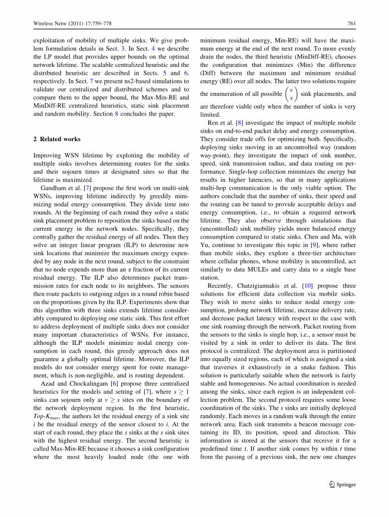
Figure 1 illustrates the need for transient configurations
in a scenario with six sinks. Moving from configuration ci
to configuration ci?1 by simply deactivating all sinks and
letting them move to their new sites would not leave any
sink active, as required. To go from ci to ci?1, we use 2
transient configurations cia and ci
b. From ci, we let the sinks
in the set M1 (boxed in the figure) move, while those in
sites v1; v3 and v5 stay active. Thus cai ¼ fv1; v3; v5g.
Moving from cia to ci
b, the sinks that left sites in M1 arrive
at their new locations in cbi ¼ fv7; v9; v11g and simul-
taneously, those in cia deactivate to move. When sinks
from sites in cia arrive at their new locations in
ciþ1 � cbi ¼ fv8; v10; v12g, they activate to put the system
into configuration ci?1. In ‘‘Appendix’’ we show that at
most two transient configurations are needed to move
between any pair of configurations.
Consider a sequence C ¼ c1; c2; . . .; cL of configura-
tions, either major or transient, that provide a schedule of
sink movements that solve our problem. Configuration ci
must hold for the time to broadcast the sink site
(de)activations necessary to move from ci into ci?1 plus
the time required to move sinks to new locations for ci?1.
For a given sequence C, we denote this minimum time for
configuration ci as sCðciÞ. We also require that major
configurations hold for at least a fixed time threshold
2 One might expect that an optimal schedule will use all stationary
sinks at all times. However, there may be times when it is best not to
use one even if it is available. This is because the extra sink will affect
packet routes, possibly affecting energy balance negatively.3 If the protocol involves a training phase, i.e., a phase through which
the sensors and the sinks learn about parameters needed to start
protocol operations, ep is the energy after the training.
762 Wireless Netw (2011) 17:759–778
123

tmin � maxi sCðciÞ seconds.4 By varying the length of tmin
we can explore trade-offs between sink mobility and
network lifetime.
Our problem is formally defined as follows.
Problem formulation. Determine an ordered set Cm ¼fc0; c1; . . .; c‘g of major configurations and a time ti � tmin
for each selected configuration ci; i ¼ 0; . . .; ‘. Also
determine transient configurations Ct ¼ fca0; c
b0; c
a1; c
b1; . . .;
ca‘�1; c
b‘�1g and times ta
i ; tbi for i ¼ 0; . . .; ‘� 1. The ordered
pair of transient configurations ðcai ; c
bi Þ defines a most
direct transition between major configurations ci and ci?1.
Call the sequence of major configurations with appropri-
ately interleaved transient configurations C. If a transient
configuration c exists, then it differs from the preceding
configuration and lasts at least sCðcÞ seconds. If one or both
of the transient configurations do not exist, the configura-
tion lasts zero seconds and is equal to the configuration
preceding it. By convention, tai � tb
i , so the ‘‘b’’ configu-
ration exists only if moving between configurations ci and
ci?1 requires two transient configurations. For convenience,
let ta‘ ¼ tb
‘ ¼ 0. We wish to maximize the network lifetime
K ¼P
i20...‘ðti þ tai þ tb
i Þ.Our definition of network lifetime requires every sensor
to have enough initial energy to support all the selected
configurations for the selected amount of time. This means
that the energy paid by each node p for generating, trans-
mitting, receiving and relaying packets while in each of the
selected configurations Cm [ Ct plus the energy spent by the
node for route maintenance operations associated with
configuration changes does not exceed the nodal initial
energy ep. (Our formulation accounts for all the energy
costs incurring at the network nodes during the network
operations.) After K seconds, at least one sensor dies.
4 A mathematical model for sink mobility
In this section we describe an LP whose solution provides
an upper bound on the maximum lifetime of a sensor net-
work with s mobile sinks. The LP is a relaxation of the
mobile sinks problem. It selects a set of (major) configu-
rations and the time for each configuration. It ignores the
ordering of configurations and the transitions between them,
minimum times for configurations to hold, and energy costs
for broadcasting sink (de)activations. Since any feasible
schedule for sink movements must obey these additional
configuration constraints and the required broadcasts con-
sume sensor energy, the lifetime of a real schedule can be no
longer than the lifetime of the optimal LP solution.
The LP has only one type of variable. Let tc be the time
configuration c [ C holds. There arePs
k¼1
vk
� �ways to
place at most s sinks on v sites, which is exponential in
s. However, we can solve this LP while explicitly including
the tc variables for only a polynomial number of configu-
rations c. The rest are implicitly 0.
The LP model is:
maximizeXc2C
tc
subject to:
Xc2C
aprptc þX
q 6¼p2N;w2V
rqbpqqpwyqwctc
!� ep; 8p 2 N:
The objective function maximizes network lifetime. The
constraints require all sensors to be alive throughout the
network lifetime. Given a sensor p [ N and a configuration
c [ C, the expression in the parentheses on the left side of
the constraint for sensor p gives its energy consumption
while the system is in configuration c. More specifically,
aprp is the energy consumption per unit time for sensing,
creating and transmitting locally generated packets.
Therefore, aprptc is the total energy consumed by p in
configuration c for packets it generates. The second term
computes the energy that sensor p expends routing packets
for other sensors during configuration c. Each term in this
sum depends on the data rate rq of sensor q, which might
route through sensor p depending on sensor q’s choices of
sink and choice(s) of route. Recall that parameter yqwc
Fig. 1 Illustration of calculating a two-step transition between major
configurations ci and ci?1. The sinks in set M1 (one element from each
matched pair in ci) deactivate and move while the remaining sinks
stay in configuration cia. The sinks originally in M1 appear in
configuration cib at locations M2, which represent one element from
each matched pair in the new configuration ci?1
4 Holding major configurations for a longer time allows routes to
stabilize and run for enough time to justify the cost of changing the
configuration.
Wireless Netw (2011) 17:759–778 763
123

indicates the fraction of sensor q’s traffic that goes to site
w in configuration c (choice of sink). We have yqwc [ 0
only if a sink sojourns at site w in configuration c and
sensor q sends packets to a sink at site w in configuration
c. Also recall parameter qqpw is the fraction of q’s traffic to
sink w that passes through sensor p (choice of route).
Therefore, rqbpqqpwyqwctc represents the energy consumed
at node p for relaying packets generated by q during the
time that configuration c holds.
4.1 Solving the LP
We will use a general method for solving LPs that have an
exponential number of constraints but a polynomial num-
ber of variables. Our LP has an exponential number of
variables, but a polynomial number of constraints. So we
will optimize our LP (the primal) by instead optimizing its
dual [11]. This is another LP, derived mechanically from
the primal, which switches the optimization direction (in
this case to a minimization). Each constraint in the primal
corresponds to a variable in the dual and each variable in
the primal corresponds to a constraint in the dual. So the
dual of our LP has an exponential number of constraints
rather than an exponential number of variables. The
objectives of the two LPs are equal at optimality. The dual
of our LP is:
minimizeXp2N
epup
subject to:
Pp2N
up rpap þP
q 6¼p2N
Pw2V
rqbpqqpwyqwc
!� 1
8c 2 C;up � 0 8p 2 N:
We can satisfy an exponential-size set of constraints by
only explicitly enforcing a polynomial number of them
provided we have a separation algorithm. Suppose we wish
to enforce a set of constraints X . A separation algorithm
accepts a solution vector for the LP that only explicitly lists
a subset of the constraints. It returns a constraint x 2 X that
is violated, or verifies all are satisfied. As a theoretical
results, such a separation procedure, when combined with
the ellipsoid algorithm, is guaranteed to converge to the
optimal LP solution in a polynomial number of iterations.
See [12–14] and especially [15, Chap. 14], for some of
many discussions of this technique.
Although it has good theoretical bounds, the ellipsoid
algorithm is not very fast. That is why linear programming
solvers use simplex or barrier methods rather than the
theoretically good ellipsoid algorithm for linear program-
ming. Similarly, we use a different, simple approach for
solving our linear program with separation. This method is
typically much better than using ellipsoid in practice.
To use a separation algorithm to solve a large LP, we
begin by explicitly listing a small (possibly empty) subset
of the constraints in X . We then solve the LP and pass the
solution to the separation algorithm. If all the constraints
are satisfied, we are done. The separation algorithm has
given a computational proof that all the constraints are
satisfied and thus all unlisted constraints are redundant at
optimality. Otherwise, we add the violated constraint it
returns, solve the new LP, and so on.
An efficient separation algorithm must exploit structure
of the constraint family; it does not enumerate the con-
straints. Thus, a separation algorithm is customized for
each problem, and there is no reason to believe a priori that
this computation is tractable. We now describe how we can
apply this approach to solving our dual LP.
Given a solution u* to the dual LP, we wish to find a
most violated constraint, or determine that all are satisfied.
One can separate by just finding any violated constraint,
but finding a most violated constraint has better conver-
gence properties. A violated constraint has the form
Xp2N
u�p rpap þX
q 6¼p2N
Xw2V
rqbpqqpwyqwc
!\1
for some configuration c. A most violated constraint
minimizes the value ofXp2N
u�pX
q6¼p2N
Xw2V
rqbpqqpwyqwc
over all configurations c. If this value is strictly less than
1�P
p2N u�prpap, then the constraint is violated and
otherwise, all are satisfied.
Since we seek a configuration, the yqwc are now vari-
ables. We can drop the c in the subscript, since we are
computing a single configuration. Defining constant
hqw ¼ rq
Xp6¼q
u�pbpqqpw;
our objective becomes minimizeP
q2N
Pw2V hqwyqw.
To find the optimal configuration, we must place up to
s sinks. We use a decision variable xw, which is 1 if there is
an active sink at site w and 0 otherwise. As before, yqw [ 0
if sensor q sends to an active sink at site w for the con-
figuration we are building. Since there must be an active
sink at site w to receive traffic, we must ensure that yqw [ 0
only if there is a sink at site w. The full separation for-
mulation, which we call SEP, becomes:
minimizeXq2N
Xw2V
hqwyqw
subject to:
764 Wireless Netw (2011) 17:759–778
123

Pw2V
xw � sPw2V
yqw ¼ 1 8q 2 N
yqw � xw 8q 2 N;w 2 Vxi 2 f0; 1g:
The first constraint enforces the sink limit. The second set
of constraints ensures that each sensor sends all its traffic to
a set of sinks. The third set of constraints ensures that
sensors send data only to a sink site that has an active sink.
That is, if xw = 0, then yqw = 0 for all sensors q.
This MILP is a classic formulation for the p-median
problem [16]. In the p-median problem, we wish to place
p facilities on any of n locations. Each of m customers must
be served by an open facility, or a mix of open facilities.
There is a service cost cij for facility i to serve customer
j. If facility i serves an xij fraction of customer j’s
requirement, this costs cijxij. The goal is to minimize the
total service cost. For our separation algorithm
p ¼ s; n ¼ jVj, and m = |N|. This separation algorithm
finds the configuration with the minimum total energy
drain (summed over all sensors) when the energy cost is
scaled by up*.
The p-median problem is NP-complete. However, there
are exact algorithms based on math-programming formu-
lations that can effectively solve problems with ten thou-
sand or more nodes and hundreds of thousands of
customers [17]. This is well within or beyond the range of
current sensor network sizes. Thus, although we cannot
solve the LP in guaranteed polynomial time, we can solve
it in practice for the sizes of LP we require, i.e., we can
compute an upper bound on WSN lifetime.
The method above works for any possible assignment of
sensors to the sinks to which they send their data. For
instance, the network owner may decide to have the sensors
send their packets to the closest sink, may forbid a source
to send to a given sink due to latency constraints, or may
list the preferred sinks according to a given ranking.
For sensor q and sink site w, let Rqw be the set of sink
sites u = w that are lower priority choices for sensor
q than site w. For example, if we must ensure that sensor
q sends only to a closest active sink, we can let d(q, w) be
the minimum distance (in hops) from sensor q to sink site
w. Then Rqw includes the set of sink sites u such that
d(q, u) [ d(q, w), i.e., those that are farther away from
sensor q than site w is. If there are ties for closest sink site,
we can let the LP choose the best way to divide traffic
among those sinks for a particular configuration. Alterna-
tively, we can extend the Rqw sets to enforce a total order
by including sites u such that d(q, u) = d(q, w) where
w has a higher ID than u (u loses the tie breaker with w). In
order to enforce this sink selection strategy we add the
following constraint to the SEP mixed-integer program:
Xu2Rqw
yqu � 1� xw 8q 2 N;w 2 V :
This set of constraints enforces priority, for example to
require sensor q to send to a closest sink. If there is an active
sink at site w (i.e., xw = 1), then q cannot send to any sink in
Rqw. Thus all the sink selection variables corresponding to
sites in Rqw will be 0. Adding the constraints to select a
closest open facility preferentially leads to a more con-
strained p-median problem. Fortunately, this slightly-mod-
ified version appears to be quite tractable for our data sets.
We can also enforce any specific set of yqwc choices for
a tractably-sized set of configurations c [ C. Suppose the
separation algorithm returns a configuration c with choices
of yqwc that do not match those given by the network
owner. We first check to see if the constraint is still vio-
lated with the correct yqwc parameters. If so, we add the
new constraint using the correct y values. If it is not vio-
lated, we will try again, forbidding the separation MILP
from returning the same precise set of sinks. Suppose
configuration c has the s sinks in locations w1;w2; . . .;ws.
To forbid the SEP integer program from returning the same
configuration, add the following constraint:
Xs
i¼1
xwi� s� 1:
This means at least one of the s variables representing this
set of sink sites must be 0 (not selected). This mechanism
could for instance be exploited to forbid configurations that
may overload some of the sinks.
5 Centralized heuristic
In this section, we describe a centralized heuristic that
begins with the solution to the LP described in Sect. 4 and
finds a feasible schedule for sink movements.
The heuristic chooses a subset of the configurations
chosen by the LP as major configurations. It must order
these major configurations and compute transitions
between neighboring major configurations. The centralized
heuristic must also determine the time each configuration
holds such that all sensors have enough energy to serve all
the configurations. Major configurations must hold for at
least tmin seconds and transient configurations must hold
long enough to complete the required broadcasts and sink
movements. The high-level operations of the centralized
heuristic are as follows:
1. Solve the LP to obtain a solution tc*. Let B = tmin.
2. Let C � C ¼ fc 2 Cjt�c � Bg. That is, we select the set
of configurations for which the LP assigns a time of at
least B (initially tmin).
Wireless Netw (2011) 17:759–778 765
123

3. Order the configurations in C, preferably with adjacent
configurations sharing some common sink sites. (This
decreases the number of transient configurations that
need to be added.)
4. Compute transient configurations between each pair of
adjacent configurations.
5. Solve another final LP (LPF) to adjust the times for
each configuration, enforce minimum times on con-
figurations, and account for sink-movement broadcast
costs.
6. If LPF is infeasible, increase B (e.g., to drop the
configuration(s) with the shortest time from C) and
return to step 2.
We now consider each step of the centralized algorithm,
starting with step 3. We use a simple traveling salesperson
(TSP) model on a graph where vertices represent the major
configurations from the LP and where there is an edge
between each pair of vertices. The edge ðci; cjÞ is weighted
by 1 plus the minimum number of transitions needed to
move from ci to cj or vice versa, since this relationship is
symmetric. The weights are 1, 2, or 3 given that at most
two transient configurations are needed to go from a major
configuration to the following one.5 We wish to find a
traveling salesman path (not a closed tour) among the
chosen configurations. The optimal TSP minimizes the
number of configurations we must add. These are tiny and
easy problems for the free TSP code Concorde [18]. If we
would like the heuristic to run in guaranteed polynomial
time, we can approximate the optimal path using Christo-
fides’ heuristic for the symmetric TSP [19].
We now give a high-level description of how to compute
the transient configuration(s) between two major configu-
rations in step 4. If there are no intermediate transitions
required, then we are done. If there is one intermediate
transition, then this usually is the (non-empty) intersection
of sites in the two major configurations. When the transi-
tion requires two transient configurations, there are many
possible choices for the transient configurations. The sink
movement schedule has the form ci;M ci; L ciþ1; ciþ1,
where ci and ci?1 are adjacent major configurations after
step 3. We must choose a set of sinks to move first, leaving
the remainder (M) behind to receive messages, and com-
pute which sites in the new configuration this set will
occupy (L). The way L and M are chosen ensures that
transient configurations induce an energy consumption
pattern similar to that of ci and ci?1. In this way, as a
whole, transient configurations show the same energy
balancing properties of major configurations. Details are
given in ‘‘Appendix’’.
We now consider the final LP. Because we have selected
the precise set of configurations (steps 2–4), we now no
longer have to allow for zero values of tc. So we can
enforce minimum times for configurations. Because we
know the order of the configurations, we can account for
route maintenance costs. Specifically, each sink in the
initial configuration c0 must broadcast its activation.
Moving between ci and ci?1, all sink sites in ci � ciþ1 must
broadcast their deactivation and all sinks in ciþ1 � ci must
broadcast their activation. Each broadcast from a sink site
w [ V has a potentially different energy cost for each
sensor. Let cp be the total energy cost for sensor p for all
route maintenance operations associated with the specific
sequence of configurations. This is a constant (a function of
the predetermined set of activations and deactivations).
Thus ep � cp is the energy sensor p has remaining for
handling packets during the network lifetime. Let Cm be the
last set of major configurations selected in step 2, let Ct be
the set of transient configurations computed in step 4, and
let C be the appropriately interleaved sequence of Cm and Ct
Then the final LP, called LPF, is as follows:
maximizeX
c2Cm[Ct
tc
subject to:
Xc2Cm[Ct
aprptc þX
q2N;w2V
rqbpqqpwyqwctc
!� ep � cp
8p 2 N
tc � tmin 8c 2 Cm
tc � sCðcÞ 8c 2 Ct:
This LP has a polynomial number of configurations so we
can solve it directly.
6 Distributed heuristics
In this section we introduce three distributed heuristics for
sink mobility. The first one takes into account the nodal
residual energy for deciding where to move the sinks. The
second and third instead move each sink randomly and
uniformly through the available sites. (The latter represent
protocols where mobility is uncontrolled and uncoordi-
nated. We will use them in the next section for
benchmarking.)
6.1 Controlled and coordinated sink mobility
The distributed heuristic for sink mobility, called DIS,
starts by placing s [ 1 sinks at any s of the v sites (initial
configuration). The sinks then broadcast a packet to the
nodes advertising their current position. Upon receiving
5 Note that these weights are a metric. Weighting only by the number
of transient states does not satisfy the triangle inequality.
766 Wireless Netw (2011) 17:759–778
123

this packet, nodes set up routes to their preferred sink
according to a selected routing protocol. Each sink main-
tains estimates of the state of the network, such as energy
level of the sensors, current traffic from the nodes sending
to it, sink locations and travel information. Based on this
information each sink guesses the network lifetime if all
sinks remain in their current positions till the network dies.
Periodically (i.e., every tmin seconds) each sink decides
whether to move or not. Based on its current estimates of
the network information, it computes the expected change
in lifetime if it were to move to another site not currently
occupied or about to be occupied by another sink. If sites
exist such that moving to one of those sites would extend
the network lifetime more than dtmin seconds, the sink
performs the following operations: It chooses the new site
which induces the maximum expected network lifetime; It
communicates to all the other sinks that it has decided to
move to the selected new site; It tells the sensors currently
reporting to it that it is on the move, shutting down the
routes to its current site (sink deactivation), and moves to
the new site. Upon arriving at the new site the sink
broadcasts a packet advertising its new position thereby
triggering route construction from the nodes for which it is
the preferred sink (sink activation).
The sinks are aware of each other’s status. Therefore a
sink knows if all the other sinks are traveling. If a sink is
the last active sink, it will wait for an activation message
before moving. This ensures that there is always a sink to
receive packets, which enables low latencies.
A sink f’s periodic decision about whether to move or
not depends on information about the state of the network.
In order to determine whether the network lifetime will be
longer if it moves, f needs to know the nodal residual
energy, the nodal data rate and the energy needed to
communicate packets in the new configuration. Sink
f learns this information either by collecting it from its
nodes, or by receiving it from fellow sinks. Sinks collect
information about current nodal energy in the following
way. The energy is divided into a constant number of
levels. When the energy of a node decreases from a level to
a lower one, a node piggybacks this information to a data
packet. A sink also gathers information about its nodes’
data rate by counting packets. Sinks periodically share this
information with the other sinks. The energy costs incurred
by a node in the new configuration are based on knowing
which node will transmit to which sink in the new con-
figuration, and on the energy cost associated with these
transmissions. The first information depends on the rank of
a given sink site in the priority list of a sender node, and the
second on estimates of the qqpw (as defined in Sect. 4). Both
priority lists and qqpw estimates are obtained at network set
up, during a training phase. This phase can be performed
by one sink, which can then share the information with all
the others. The sink travels to each sink site and broadcasts
a packet to make the sensor nodes aware of its current
location. Upon receiving this packet the sensor nodes
transmit test packets to the sink according to the routing
protocol in use. Each test packet carries information about
the route followed from its source to the current location of
the sink. Each traversed hop is associated with the energy
necessary to forward the packet through it. After receiving
a few test packets from a node q, a sink sojourning at site
w is able to estimate, for each node p, the fraction of
packets generated by q that will be relayed by p when
q transmits to a sink at that site (i.e., the sink is able to
estimate qqpw). A sink at w knows the energy consumption
needed by node p to relay packets from q. During the
training phase, sensor nodes also decide how good a sink
site is for them, and return this information to the sink in
the test packets. Therefore, a node creates a priority list of
sink sites.
6.2 Random mobility: RND and ZRND
We define two sink mobility scheme intended to represent
uncontrolled mobility.
The first scheme, called RND (for random scheme),
works as follows. Every tmin seconds, a sink randomly and
uniformly decides the next site to visit among all unoccu-
pied sites and its current site. If the sink moves to a new
site, it communicates its decision to its peers, so that no two
sinks go to the same site. Sensor-to-sink multi-hop route
management and sink movement coordination happens as
for DIS.
In ZRND (for zone random scheme) instead, the
deployment area is divided into s zones, each associated to
a given sink (and only to it, i.e., the zones are non-over-
lapping). Every tmin seconds the sink randomly and uni-
formly selects the next site among the ones in its own zone.
7 Performance evaluation
In this section we discuss the results of a simulation-based
performance evaluation of the solutions proposed in this
paper. The section is organized into three parts. We first
introduce the simulators, the simulation scenarios and their
parameters. Then, we compare the performance of our
distributed heuristic DIS and of the centralized heuristic
(CEN in the following) defined in Sect. 4 to the upper
bound on the optimal network lifetime (OPT), and to
lifetimes for random sink mobility (RND and ZRND) and
for optimally placed static sinks (STATIC). Finally, we
compare the performance of our solutions to the perfor-
mance of the solutions for multiple sink mobility Max-
Min-RE and MinDiff-RE presented in [6].
Wireless Netw (2011) 17:759–778 767
123

7.1 Simulators and simulation scenarios
The results for OPT have been obtained by solving the LP
model defined in Sect. 4 with the commercial solver
CPLEX [20] run on Linux-based 64bit dual-core comput-
ers. The various runs took from few hours to few days to
produce results. We considered the two cases where the
sensors send their data to the closest sink, or to the ‘‘best’’
sink, which is the one sending to whom maximizes network
lifetime. The first choice comes as a natural one in the
sense that is very easy to implement by all the heuristics,
and it is the default one in our experiments.
We implemented the centralized heuristic CEN (Sect. 5)
in a home-grown software framework made up of Perl
scripts [21], the freely available Concorde TSP solver [18],
and the solver for the maximum weight matching problem
based on the N-cubed weighted matching algorithm by
Gabow [22]. The latter is available through Mathprog at
DIMACS (http://www.dimacs.rutgers.edu). In all the con-
sidered scenarios steps two through four of CEN were
extremely fast, never lasting more than one second. The
more time consuming operation was running LPF which
however never took more than three hours on an Intel dual-
core 1.86 GHz workstation with Linux OS and 16 GB of
RAM. We implemented DIS, RND, ZRND, STATIC, and
Max-Min-RE and MinDiff-RE in ns2 [23] with the
parameters listed below. Our simulations also take into
account all the overhead generated by every possible pro-
tocol operation. We used simulations to derive the energy
costs for packet communication and route management, as
well as the estimates for the qqpw parameters that the
analytical frameworks for OPT and CEN require.
All our experiments consider realistic parameters of
WSNs. There are 400 wireless sensor nodes deployed over
a square area of side L. Each node transmission radius is
25 m. Each node has an initial energy of 50 J. It generates
512 B packets at the rate r ¼ 0:5 bps and sends them to
the selected sink according to a (hop-based or geographic)
shortest path routing. The channel data rate is 250 Kbps
(consistent with IEEE 802.15.4 [24]). The transmission
power and the receiving power are 0.0144 and 0.0125 W,
respectively, according to the specifications of the TR 1000
radio transceiver from RF Monolithics [25]. We do not
consider sleep or idle power consumption. We assume that
when not transmitting or receiving packets, node radios are
in sleep mode, i.e., consume a negligible fraction of the
energy required when the radio is up (we can use an
on-board wake-up low-power radio like that described in
[26–28], which wakes up a node from sleep mode only
when it has a packet to receive).
Sinks are free to move from any of the sites of a 4 4
and 8 8 grid to any other site of the grid. They are
resource-rich devices, and we assume that sinks can
communicate among themselves through high-data rate
reliable communications. We vary the number of sinks in
the range [2, 8]. Protocol related parameters are configured
as follows. The mandatory time sinks are forced to sojourn
at a site in a major configuration (tmin) varies in the set {50,
100, 250} Ks. The threshold d that governs a sink move-
ment decision is 0.1. Finally, nodal energy is partitioned
into 40 levels, each being 2.5% of the initial energy.
To test our solutions we have considered two different
nodal deployments: Nodes are either placed on a grid or
they are scattered randomly and uniformly throughout the
area. In the first case the 400 nodes are placed on a 20 20 regular grid within a deployment area of side
L ¼ 475 m. The selected transmission radius (25 m)
ensures that every non-border node has exactly four
neighbors. In these scenarios the selected routing is shortest
path, and each node sends its packets to the closest sink. In
the second case, L is set to 300 m. This induces an average
network density of 8.15 neighbors per node. The two dif-
ferent deployments allow us to explore the effect of dif-
ferent densities and different energy consumption patterns
on our solutions (see Sect. 7.2.2)
The results we present here are obtained by running 100
experiments for each displayed value. (The 95% confi-
dence interval is depicted in the figures and displayed along
with the data on the tables.)
7.2 Performance evaluation of the proposed heuristics
7.2.1 Grid deployment of the sensor nodes
We start by considering 400 nodes deployed on a 20 20
grid. The nodal transmission range is 25 m and the side of
the square deployment area is 475 m.
Tables 1 and 2 show the network lifetime induced by the
various protocols when varying tmin, the number s of sinks,
and the number of sink sites v. The network lifetime is
defined here as the time till energy depletion of the first
sensor. Each table entry shows the absolute lifetime (in
millions of seconds) and the percentage decrease with
respect to OPT (in parentheses). For ZRND we show
results with 2k (0 \ k � 3) moving sinks because in this
case it is possible to divide the deployment area into 2k
identical square regions.
The centralized heuristic CEN achieves network life-
times that are remarkably close to the optimum: The gap
from OPT is always below 1%. CEN does so well because
it starts from the set of (good) configurations that are
produced by OPT. CEN uses these same configurations
adding intermediate ones and selecting the times the sinks
spend in each configuration by solving LPF (Sect. 5) This
forces each selected major configuration to last at least tmin,
and the transient ones the time needed for broadcasting
768 Wireless Netw (2011) 17:759–778
123

sink activations and deactivations and for the sinks to
move. The time the sinks spend in each of these configu-
rations might, in principle, differ substantially from that
selected by OPT. However, we notice that the good con-
figurations where OPT sends the sinks for the most time are
also those selected by CEN. This is the natural conse-
quence of OPT and CEN being optimization formulations.
LPF in CEN optimizes the lifetime and deems it useful to
spend long times in those good configurations where traffic
is delivered with low energy consumption and the energy
toll is balanced among the nodes. These configurations are
the major configurations selected by OPT. The additional
configurations needed by CEN for transitioning from major
configurations are carefully selected to mimic the adjacent
major configurations. They also are short compared to
major configuration, with a limited impact on the overall
Table 1 Lifetime, in millions of seconds (and % gap from OPT), 4 4 grid
s tmin
(K)
OPT CEN DIS RND ZRND STATIC
2 50 46.71 46.71 (&0) 44.1 ± .06 (5.5) 29 ± .22 (37.9) 30.91 ± .21 (33.8) 11.1 (76.2)
100 46.71 46.71 (&0) 43.8 ± .12 (6.2) 28.8 ± .32 (38.3) 30.2 ± .33 (35.3) 11.1 (76.2)
250 46.71 46.7 (.02) 43.4 ± .12 (7) 27.4 ± .44 (41.3) 28.5 ± .41 (38.8) 11.1 (76.2)
3 50 61.14 61.1 (.01) 54 ± .2 (11.6) 38.2 ± .22 (37.5) 14.8 (75.8)
100 61.14 61.1 (.01) 53.3 ± .22 (12.8) 37.6 ± .33 (38.5) 14.8 (75.8)
250 61.14 61 (.07) 52.1 ± .33 (14.7) 35.4 ± .43 (42.1) 14.8 (75.8)
4 50 75.94 75.93 (.01) 58.5 ± .7 (22.9) 45.6 ± .24 (39.9) 50.6 ± .26 (33.3) 19.1 (74.8)
100 75.94 75.93 (.01) 57.9 ± .69 (23.7) 44.7 ± .27 (41.1) 49.9 ± .39 (34.3) 19.1 (74.8)
250 75.94 75.9 (.06) 57.8 ± .71 (23.8) 42.2 ± .46 (44.4) 48.1 ± .51 (36.6) 19.1 (74.8)
5 50 82.42 82.41 (.01) 62.9 ± .25 (23.6) 50.8 ± .27 (38.3) 22.3 (72.9)
100 82.42 82.41 (.01) 62.4 ± .32 (24.2) 50.2 ± .33 (39) 22.3 (72.9)
250 82.42 82.41 (.17) 61.5 ± .33 (25.3) 48.5 ± .48 (41.1) 22.3 (72.9)
6 50 84.97 84.96 (.01) 67.9 ± .31 (20) 55.6 ± .3 (34.5) 28.8 (66.1)
100 84.97 84.96 (.01) 67.5 ± .28 (20.5) 55 ± .4 (35.2) 28.8 (66.1)
250 84.97 84.96 (.01) 67.3 ± .36 (20.7) 53.7 ± .52 (36.8) 28.8 (66.1)
7 50 87.29 87.28 (&0) 73.2 ± .23 (16.1) 60.2 ± .26 (31) 33.7 (61.3)
100 87.29 87.28 (&0) 72.9 ± .28 (16.4) 59.7 ± .34 (31.6) 33.7 (61.3)
250 87.29 87.27 (.02) 72.4 ± .26 (17) 58.1 ± .44 (33.4) 33.7 (61.3)
8 50 88.96 88.9 (&0) 76.5 ± .31 (14) 63.4 ± .22 (28.7) 59.6 ± .23 (33) 45.2 (49.2)
100 88.96 88.9 (&0) 76.1 ± .32 (14.4) 63.1 ± .31 (29) 59.2 ± .3 (33.4) 45.2 (49.2)
250 88.96 88.9 (&0) 75.4 ± .41 (15.2) 61.6 ± .45 (30.7) 59 ± .43 (33.6) 45.2 (49.2)
Table 2 Lifetime, in millions of seconds (and % gap from OPT), 8 8 grid
s tmin
(K)
OPT CEN DIS RND ZRND STATIC
2 50 79.51 79.49 (.02) 68.5 ± .42 (13.8) 39.2 ± .28 (50.7) 47.4 ± .32 (40.3) 14.2 (82.1)
100 79.51 79.49 (.02) 67.8 ± .4 (14.7) 39.2 ± .37 (50.7) 46.5 ± .38 (41.4) 14.2 (82.1)
250 79.51 79.2 (.4) 64 ± .75 (19.5) 38 ± .62 (52.2) 43.9 ± .6 (45.2) 14.2 (82.1)
3 50 105.9 105.9 (.03) 90.1 ± .36 (14.9) 50.7 ± .36 (52.1) 20.8 (80.3)
100 105.9 105.9 (.03) 89.3 ± .32 (15.6) 50.7 ± .54 (52.1) 20.8 (80.3)
250 105.9 105.8 (.05) 87.6 ± .36 (17.2) 49.3 ± .8 (53.4) 20.8 (80.3)
4 50 131.4 131.4 (.03) 106.4 ± .33 (19) 63.4 ± .47 (51.7) 88 ± .26 (33) 27.7 (78.9)
100 131.4 131.4 (.04) 105.7 ± .43 (19.5) 63.6 ± .5 (51.6) 86.9 ± .41 (33.8) 27.7 (78.9)
250 131.4 131.3 (.1) 102.5 ± .64 (22) 61.5 ± .81 (53.2) 83.8 ± .63 (36.2) 27.7 (78.9)
5 50 150.1 150 (.04) 120 ± .66 (20) 75.6 ± .46 (49.6) 34.3 (77.1)
100 150.1 150 (.04) 118.8 ± .77 (20.8) 75.9 ± .62 (49.4) 34.3 (77.1)
250 150.1 149.9 (.1) 117 ± .51 (22) 73.9 ± .93 (50.7) 34.3 (77.1)
Wireless Netw (2011) 17:759–778 769
123
energy consumption. This explains the near-optimal per-
formance of the centralized heuristic (as mentioned, just
\1% from OPT).
One may wonder how much OPT and CEN loose
making nodes sending their packets to the closest sink
rather than to the best one. To answer this question we have
run the model by setting this option, and observed that the
loss (in lifetime) is quite limited ranging from 3.8 to 8.7%.
The distributed heuristic DIS is aware of the residual
energy at the network nodes because of the exchange of
information among the sinks. Based on this (approximate)
knowledge as well as on the estimate of the nodal data rate
and of the energy consumption pattern, DIS can move the
sinks to configurations that are expected to improve net-
work lifetime. Traffic and energy-awareness pay off in
terms of network lifetime, which is always within 25.3%
from the OPT lifetime. Equally important, the improve-
ment with respect to STATIC is as high as fourfold. This
confirms the goodness of exploiting controlled, energy-
aware sink mobility, especially for multiple sinks.
Sink mobility is advantageous even when uncontrolled,
i.e., even when sink movements do not depend on the
network state (nodal residual energy, energy consumption
patterns, etc.). With RND the random movements of the
sinks almost triples the network lifetime with respect to
STATIC. ZRND offers similar performance.
We also observe that OPT and the other heuristics
induce longer lifetimes when the number of sinks increa-
ses. This is because the network traffic is partitioned
among a larger set of sinks, sink neighbors receive fewer
packets, routes are shorter and the overall energy con-
sumption is lower. However, we notice lifetime improve-
ments which are not linear in the number of sinks. In other
words, having two sinks does not double lifetime compared
to one sink. Having three sinks does not triple lifetime, and
so on. This is evident in Table 1, which shows that
deploying 8 sinks only leads to a 17% improvement in
OPT lifetime with respect to scenarios with 4 sinks. Given
our set of sink sites, we do not expect that linear
improvement is possible. The route length and the overall
energy consumption do not halve when we double the
number of sinks. In addition, achieving linear improve-
ments would require sinks to be assigned (on average) to
configurations which perfectly partition data sources to the
sinks. Such perfect configurations are rare, if possible at
all. Moreover, if it were possible for sinks to transition only
among this kind of node-balanced configurations it would
be challenging to obtain good energy balancing. Energy
balancing is in fact the consequence of the fine tuning of
the time spent by the sinks in different configurations
(including unbalanced ones) so that all the nodes relay a
similar amount of traffic over time and the energy con-
sumption is minimized.
For all protocols, remarkably higher lifetime is obtained
by increasing the number of sink sites v. For example,
when 5 sinks may visit 64 sites the lifetime is 150.1 Ms for
OPT. When restricted to 16 sink sites the lifetime is
82.42 Ms. A higher number of sites allows the protocol to
choose among a higher number of configurations. Denser
sink sites allow the sinks to drain energy from all the dif-
ferent areas in the network.
We finally observe that both DIS, RND and ZRND
produce higher lifetime increases as tmin decreases. The
reason is that higher tmins result in a coarser selection of the
times spent in the various configurations, and therefore in a
worse energy balancing. In addition, the price to pay for
having entered an ‘‘energy undesirable’’ configuration is
paid for a longer time.
As a final remark, we observe that our mobility schemes
not only improve the average network lifetime, but also
consistently perform well in every single run we consid-
ered. For instance, in the case with 4 sinks moving among
16 sites and tmin = 50,000 s the minimum network lifetime
for DIS is 54.6 Ms, a mere 7% from the observed average.
In the case with 5 sinks moving over 64 sink sites, and
tmin = 50,000 s, the average lifetime is 11% greater than
the observed minimum. These two cases are those with the
greatest standard deviation of network lifetime for the 16
and 64 scenarios, respectively (in all other scenarios the
variance is even smaller).
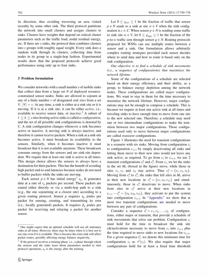
Beyond achieving improved network lifetime CEN and
DIS also result in a more even distribution of the nodes
residual energies with respect to RND, ZRND and STATIC
(confirming they are able to more evenly distribute the
traffic load over different nodes throughout the network
lifetime). Ideally, we would like the sinks to coordinately
move, changing their positions over time so that the energy
is evenly drained from all the areas in the networks. CEN
and DIS satisfactorily achieve our goal. This is clearly
shown in Fig. 2 which displays the residual energy of the
nodes at network lifetime. The figure shows the results of a
run on a typical scenario where 5 sinks can select among 64
sites (performance does not significantly change when
considering different runs). A lighter color means a lower
percentage of residual energy in that area of the network.
We observe that CEN results in better energy balancing
that DIS, which in turn outperforms RND, ZRND and
STATIC. More precisely, at lifetime OPT and CEN show
an impressive percentage of nodes with very little energy
left, a witness of its good energy drainage balancing
property. The fraction of nodes with less than 20% (40%)
residual energy at network lifetime is 52.5% (80%). This
means that at network lifetime, i.e., when the first sensor
dies, many more sensors are also about to cease their
operations, which comprises the functioning of the whole
network. Specifically, in all considered scenarios we
770 Wireless Netw (2011) 17:759–778
123

observed that from 73 to 96% of the nodes around all sink
sites (the only ones that can relay packets to the sinks) are
left with no more than 3% of their initial energy, which
makes communications very limited if not impossible.
In DIS the percentage of nodes with less than 20% of the
initial energy at lifetime is around 36.7%. The percentage
of nodes with less than 40% of the initial energy is 57.2%.
These figures reduce to 12.75 and 39.75% for RND-
induced residual energy, and to 1.75 and 3.5% for STA-
TIC. In a scenario with 4 moving sinks, these figures for
ZRND equates 16 and 52.5%.
The other WSN-relevant metric we have investigated is
the end-to-end packet latency (Tables 3, 4). For all proto-
cols, latencies are quite low, never exceeding 200 ms (the
worst case is RND, 16 sinks site, 2 sinks scenario).
Latency performance mostly depends on the average
length of the routes traveled by packets. Increasing the
number of sinks results in lower route length, and therefore
in lower latencies.
When comparing the end-to-end latency experienced by
the different schemes, we observe that STATIC achieves
the shortest routes almost always because it places the
sinks in a well balanced way resulting in short source-to-
sink routes. CEN and DIS select configurations which
spread sinks over different areas in the network, more or
less evenly associating nodes to the different sinks. The
increase of route length and end-to-end latency of CEN and
DIS over STATIC is therefore quite limited, never more
than 18% (for 16 sink sites) or more than 20% (for 64 sink
sites). Both heuristics have comparable performance,
interchangeably outperforming each other depending on
the specific scenario. RND can produce configurations
where the sinks are all on one side of the network, thus
inducing sensor-to-sink routes that can be long, and thus
again longer latencies. In our scenarios we measured an
increase of end-to-end latency of up to 12% with respect to
CEN and DIS. ZRND mitigates the unbalanced effects
observed for RND, producing latencies that are similar to
DIS.
We notice that the above end-to-end packet latency
increases/decreases have very limited impact on perceived
performance (we are speaking of latencies of few hundred
milliseconds) while the increases in network lifetime
obtained by energy-aware solutions like DIS (over RND,
ZRND and STATIC) make a remarkable difference in
terms of the monitoring capability of the network. For
instance, in the 16 sink site scenario with 2 sinks (see
Table 1), DIS is able to successfully deliver over two
million packets during the network lifetime vs. the half a
million packets that are delivered in STATIC scenarios.
The number of DIS-delivered packets is 3.7 millions and
those delivered in STATIC scenario are 2.2 when 8 sinks
roam through the network.
Finally, we have run experiments where packets are
routed to the sinks through geographic routing (namely,
geographic greedy forwarding). We observed trends and
values similar to those obtained with shortest path routing.
For instance, in scenarios with 8 (4) sinks traveling through
16 sink sites, OPT achieves a lifetime of 89.5 Ms
(78.7 Ms) when using geographic routing vs. a lifetime of
88.96 Ms (75.93 Ms) obtained by routing packets via
shortest paths.
0
20
40
60
80
100
(a) CEN 0
20
40
60
80
100
(b) DIS
0
20
40
60
80
100
(c) RND 0
20
40
60
80
100
(d) STATIC
Fig. 2 Residual energy at lifetime for CEN (a), DIS (b), RND (c),
and STATIC (d), 5 sinks in a 8 8 grid
Table 3 End-to-end packet latency, in seconds (4 4 grid)
s CEN DIS RND ZRND STATIC
2 .189 .19 .2 .19 .166
3 .153 .15 .166 .129
4 .129 .131 .141 .13 .123
5 .117 .112 .124 .105
6 .107 .103 .112 .105
7 .097 .096 .103 .091
8 .089 .09 .094 .09 .082
Table 4 End-to-end packet latency, in seconds (8 8 grid)
s CEN DIS RND ZRND STATIC
2 .179 .177 .196 .18 .154
3 .139 .138 .16 .117
4 .116 .112 .137 .122 .096
5 .102 .102 .122 .087
Wireless Netw (2011) 17:759–778 771
123

7.2.2 Random and uniform sensor deployment
In this section we explore the performance of the solutions
we proposed when nodes are randomly and uniformly
deployed. We consider scenarios where 400 nodes are
scattered randomly and uniformly throughout a square area
of side L ¼ 300 m. As previously considered, the sensor
node transmission radius is 25 m and the sink sites are
deployed in a grid pattern. Packet are routed to the closest
sink via shortest paths. We tested 12 different connected
topologies, running multiple experiments on each one. The
average nodal degree of the considered topologies varies
from 7.51 to 8.46 (doubling that of the grid case). We
investigated scenarios where 2, 3 and 4 sinks roam through
the network nodes, sojourning at v sink sites, with v ¼ 16
and 36.
A different deployment and different (i.e., higher) den-
sities considerably affect nodal energy consumption. In
particular, the average energy consumed by a node is
considerably reduced. For instance, while the nodal aver-
age consumption per second is 4.53E-7J in the case of grid
deployment, when nodes are scattered randomly and uni-
formly the same metric averages to 2.81E-7J (with 2 sinks
roaming over a 4 4 sink-site grid). The averages become
3.3E-7 and 2.05E-7, respectively, when we deploy four
mobile sinks. Nodal deployment also affects routing, thus
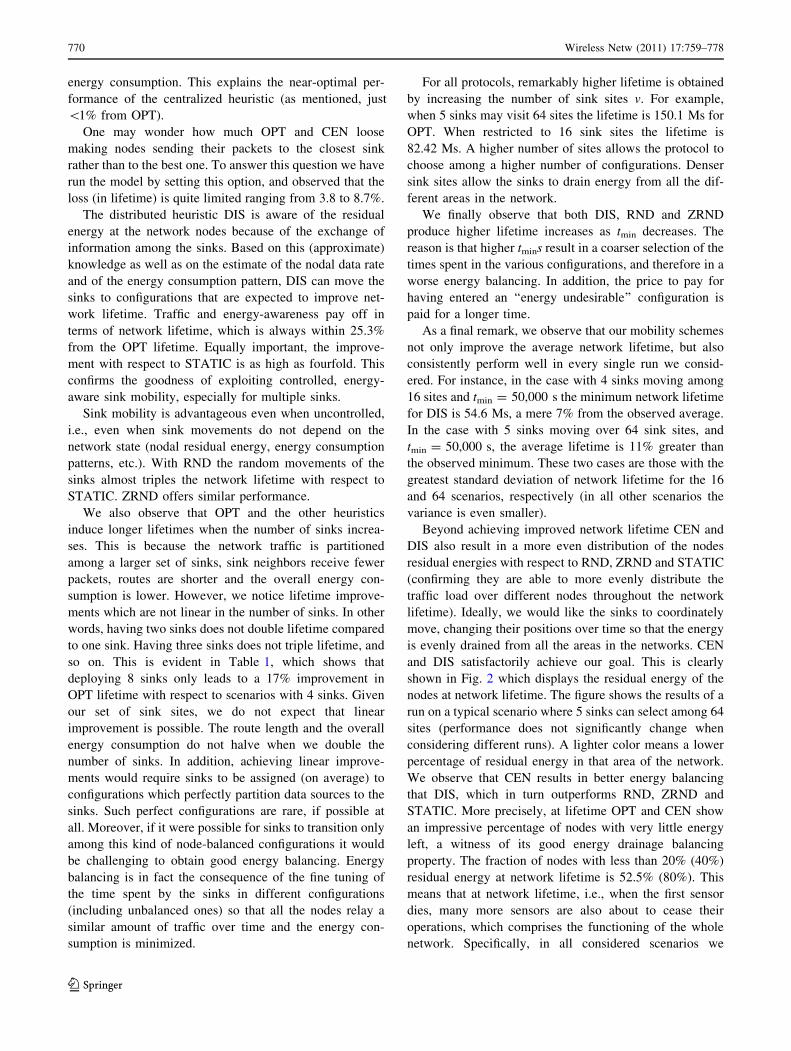
inducing different energy consumption patterns. Figure 3
shows the different patterns of energy consumption
imposed by routing over different types of nodal deploy-
ment when two sinks (red circles) are positioned at two
opposite corners of the network. The squares represent
sensor nodes. Different shades of gray indicate different
energy consumption rates per node (J/s): The darker the
node the higher the energy consumed per second.
Figure 3 demonstrates that in the grid deployment the
nodes that are stressed the most are the immediate neigh-
bors of a sink, and the energy consumption rate is quite
regular (Fig. 3(a)). When nodes are scattered randomly and
uniformly throughout the area (Fig. 3(b)), critical nodes are
bottlenecks in the (non-necessarily radio) vicinity of the
sink, and the energy consumption patterns are more
irregular. (We have observed similar trends with different
configurations.)
Despite these significant differences, our experiments
show that the relative trends of the different protocols in
terms of the metrics of interest (network lifetime, packet
route length and end-to-end latency) are the same whether
the sensors are deployed on a grid or randomly and
uniformly.
This is clearly indicated by the results shown in Tables 5
and 6 for the lifetime and in Tables 7 and 8 for the end-to-
end packet latency.
We observe that the values obtained for network lifetime
are comparable to those observed for the grid deployment
scenario (e.g., Table 1). This is because, despite higher
density usually enables better balancing and lower per node
energy consumption, moving sinks so that energy con-
sumption is balanced and minimized is much more chal-
lenging, given the irregular nodal placement. This
motivates a more uneven distribution of nodal residual
energy at lifetime in all protocols, including CEN.
For instance, when 4 sinks move in a 6 6 grid, the
fraction of CEN nodes with less than 20% (40%) residual
energy at network lifetime is 19.64% (32.45%). The per-
centage of CEN nodes with less than 60% (80%) of the
initial energy is 49.54% (73.46%). In DIS the percentage of
nodes with less than 20% (40%) of the initial energy at
lifetime is 8.86% (19.29%). The percentage of nodes with
less than 60% (80%) of the initial energy is 35.39%
(62.84%). With the RND heuristic the percentage of nodes
with less than 20% (40%) of the initial energy at lifetime is
1.03% (4.14%). The percentage of RND nodes with less
than 60% (80%) of the initial energy is 14.35% (44.8%).
With ZRND, instead, the percentage of nodes with less
than 20% (40%) of the initial energy at lifetime is 0.84%
(2.21%). The percentage of ZRND nodes with less than
60% (80%) of the initial energy is 8.31% (29.37%).
Finally, these figures drop to 1.62, 3.81, 7.66 and 16.87%,
respectively, for STATIC.
7.3 Comparative performance evaluation
We compare the lifetime of our solutions to that induced by
the heuristics Max-Min-RE and MinDiff-RE, the best
among the three sink mobility schemes presented in [6].
This shows the differences between our approach to con-
trolled and coordinated mobility and schemes that limit
sinks to sites along the network perimeter. Previous
perimeter-based solutions have effectively improved life-
time for one sink [29].
MinDiff-RE is a centralized scheme where sinks sojourn
only at sites at the boundary of the deployment area. The
protocol proceeds in rounds. At the beginning of each
round, the sinks move to a configuration that minimizes the
difference between the maximum and minimum residual
energy of the nodes at the end of the round. This difference
is computed for all possible configurations. Considering
scenarios with s sinks and v sink sites, the number of
configurations to check at each round isvs
� �, which
grows exponentially with s. This limits the applicability of
this method to networks with a limited number of sinks.
For instance, the 8 8 sink site grid scenario considered
above has 28 sink sites on the area perimeter, which force
772 Wireless Netw (2011) 17:759–778
123

thousand of configurations to be checked each round even
for s as small as 3.
Max-Min-RE differs from MinDiff-RE only in the way
the new configuration is selected at the beginning of each
round. Max-Min-RE chooses the configuration which
maximizes the minimum residual energy over all nodes at
the end of the round.
Given the scalability problems of the two heuristics, in
the following performance comparison we consider only
the 4 4 sink site grid case. Packet are routed to the
closest sink via shortest paths. All relevant parameters are
set as described as in Sect. 7.2.1 (nodes deployed on a
grid). In particular, DIS, RND, Max-Min-RE and MinDiff-
RE decide whether to move or not, and where, every tmin.
Fig. 3 Per node energy
consumption with different
types of deployment
Table 5 Lifetime, in millions of seconds (and % gap from OPT), 4 4 grid
s tmin
(K)
OPT CEN DIS RND ZRND STATIC
2 50 46.9 ± 2.3 46.9 ± 2.3 (&0) 40.2 ± 2.4 (14.3) 25.8 ± 1.8 (45) 24.3 ± 2.2 (48.2) 15.3 (67.3) ± 1.1
100 46.9 ± 2.3 46.9 ± 2.3 (&0) 40.1 ± 2.5 (14.6) 25.5 ± 1.6 (45.5) 24.1 ± 2.1 (48.6) 15.3 (67.3) ± 1.1
250 46.9 ± 2.3 46.9 ± 2.3 (&0) 39.7 ± 2.4 (15.5) 24.6 ± 1.5 (47.5) 23.4 ± 1.9 (50) 15.3 (67.3) ± 1.1
3 50 64.1 ± 3.1 64.1 ± 3.1 (&0) 53.8 ± 3.2 (16) 32.6 ± 1.9 (49.1) 20.2 (68.4) ± 1.7
100 64.1 ± 3.1 64.1 ± 3.1 (&0) 53.4 ± 3.2 (16.6) 32.5 ± 1.8 (49.3) 20.2 (68.4) ± 1.7
250 64.1 ± 3.1 64.1 ± 3.1 (&0) 52.7 ± 3.3 (17.7) 31.6 ± 1.8 (50.7) 20.2 (68.4) ± 1.7
4 50 75.3 ± 3.4 75.3 ± 3.4 (&0) 63.7 ± 3.6 (15.4) 38.2 ± 2.3 (49.2) 36.7 ± 3 (51) 24.8 (67) ± 1.8
100 75.3 ± 3.4 75.3 ± 3.4 (&0) 63.4 ± 3.6 (15.8) 38.1 ± 2.3 (49.4) 36.8 ± 3 (51) 24.8 (67) ± 1.8
250 75.3 ± 3.4 75.3 ± 3.4 (&0) 62.5 ± 3.8 (16.9) 37.2 ± 2 (50.6) 36 ± 2.7 (52) 24.8 (67) ± 1.8
Table 6 Lifetime, in millions of seconds (and % gap from OPT), 6 6 grid
s tmin
(K)
OPT CEN DIS RND ZRND STATIC
2 50 56.5 ± 2.9 56.5 ± 2.9 (.01) 45.1 ± 2.6 (20.1) 25.5 ± 1.8 (54.8) 25.1 ± 2.6 (56) 17 (69.9) ± 1.3
100 56.5 ± 2.9 56.5 ± 2.9 (.01) 45 ± 2.7 (20.3) 25.4 ± 1.7 (55) 24.9 ± 2.6 (55.8) 17 (69.9) ± 1.3
250 56.5 ± 2.9 56.5 ± 2.9 (.06) 44.6 ± 2.6 (21) 24.8 ± 1.6 (56.1) 24.5 ± 2.4 (56.6) 17 (69.9) ± 1.3
3 50 82.2 ± 2.3 82.2 ± 2.3 (.01) 64.1 ± 3.2 (22) 33.1 ± 2.4 (59.7) 37 ± 2.5 (55) 23.6 (71.2) ± 1
100 82.2 ± 2.3 82.2 ± 2.3 (.02) 63.8 ± 3 (22.3) 33.1 ± 2.3 (59.7) 36.9 ± 2.4 (55) 23.6 (71.2) ± 1
250 82.2 ± 2.3 82.2 ± 2.3 (.03) 62.9 ± 3 (23.4) 32.6 ± 2.2 (60.3) 36.5 ± 2.3 (55) 23.6 (71.2) ± 1
4 50 105.2 ± 2.1 105.2 ± 2.1 (.02) 81.9 ± 2.2 (22.1) 40.2 ± 2.8 (61.7) 42.6 ± 2.7 (60) 30.5 (71) ± 1.6
100 105.2 ± 2.1 105.2 ± 2.1 (.02) 81.3 ± 2.2 (22.7) 40.2 ± 2.8 (61.7) 42.8 ± 2.7 (60) 30.5 (71) ± 1.6
250 105.2 ± 2.1 105.2 ± 2.1 (.03) 80.2 ± 2.2 (23.8) 40.1 ± 2.5 (61.8) 42.6 ± 2.6 (60) 30.5 (71) ± 1.6
Wireless Netw (2011) 17:759–778 773
123

For fairness reasons, in the scenarios of Max-Min-RE and
MinDiff-RE the 16 sink sites are equally spaced along the
perimeter of the deployment area.
Figure 4 shows network lifetime results. We observe
that the lifetime values induced by Max-Min-RE and
MinDiff-RE mobility (the two curves are basically over-
lapping) are always remarkably worse than those of CEN
and DIS. However, Max-Min-RE and MinDiff-RE perform
comparably to RND.
The reason for the poor Max-Min-RE and MinDiff-RE
performance is limiting the sinks to move only to sites on
the boundary of the deployment area, and not within it. As
observed in scenarios where the nodes are deployed dif-
ferently (grid vs. random and uniform), combining con-
figurations that hold the sinks both on the perimeter and
inside the deployment area successfully obtains even
drainage of energy at the network node. This is a key
factor in prolonging network lifetime, which is the
objective function that we want to maximize by moving
the sinks. Following more geographic/geometric criteria as
in Max-Min-RE and MinDiff-RE and limiting through
these criteria the movement of the sinks inevitably
decreases the possibility of taking advantage of configu-
rations that help in balancing nodal energy consumption.
The values of the residual energy at lifetime confirms this
observation.
Finally, keeping the sinks on the perimeter results in
longer routes and longer latencies. In order to get to the
Table 7 End-to-end packet latency, in seconds (4 4 grid)
s tmin
(K)
CEN DIS RND ZRND STATIC
2 50 .134 ± .003 .125 ± .003 .151 ± .002 .145 ± .002 .106 ± .006
100 .133 ± .003 .125 ± .003 .15 ± .002 .145 ± .001 .106 ± .006
250 .133 ± .003 .125 ± .003 .151 ± .002 .143 ± .001 .106 ± .006
3 50 .108 ± .003 .104 ± .002 .125 ± .001 .091 ± .002
100 .108 ± .003 .104 ± .002 .124 ± .001 .091 ± .002
250 .108 ± .003 .104 ± .003 .123 ± .002 .091 ± .002
4 50 .093 ± .002 .091 ± .002 .107 ± .001 .094 ± .002 .079 ± .004
100 .094 ± .003 .091 ± .002 .106 ± .001 .095 ± .002 .079 ± .004
250 .093 ± .003 .091 ± .002 .106 ± .001 .095 ± .002 .079 ± .004
Table 8 End-to-end packet latency, in seconds (6 6 grid)
s tmin
(K)
CEN DIS RND ZRND STATIC
2 50 .124 ± .002 .118 ± .002 .144 ± .002 .136 ± .002 .102 ± .005
100 .124 ± .002 .118 ± .002 .143 ± .002 .136 ± .002 .102 ± .005
250 .124 ± .002 .118 ± .002 .142 ± .001 .137 ± .002 .102 ± .005
3 50 .099 ± .002 .096 ± .001 .118 ± .001 .112 ± .001 .086 ± .004
100 .099 ± .002 .096 ± .001 .118 ± .001 .112 ± .001 .086 ± .004
250 .099 ± .002 .096 ± .001 .117 ± .001 .112 ± .001 .086 ± .004
4 50 .085 ± .001 .083 ± .001 .102 ± .001 .09 ± .001 .076 ± .002
100 .085 ± .001 .083 ± .001 .102 ± .001 .09 ± .001 .076 ± .002
250 .085 ± .001 .083 ± .001 .102 ± .001 .09 ± .001 .076 ± .002
0
2e+07
4e+07
6e+07
8e+07
1e+08
1.2e+08
2 3 4 5 6 7 8
Lif
etim
e (s
)
Number of sinks
OPTCENDIS
RANDMax-Min-RE
MinDiff-RESTATIC
Fig. 4 Network lifetime vs. number of sinks
774 Wireless Netw (2011) 17:759–778
123

sink closest to its source, a packet has to travel a potentially
high number of hops. This results in a higher nodal energy
consumption per second (which also explains the results
obtained for the network lifetime) and in higher latencies.
8 Conclusions
We have shown that controlled and coordinated mobility of
multiple sinks effectively improves the lifetime of a WSN.
By defining a mathematical model that takes into account
realistic parameters, we have provided a provable upper
bound on the lifetime of WSNs of realistic scale (OPT).
We also defined a centralized heuristic (CEN) for con-
trolled sink mobility. It determines routes and sojourn
times for multiple sinks that depend on the network state
and produces network lifetimes remarkably close to the
upper bound. We then defined a distributed protocol (DIS)
for controlled and coordinated sink movements based on
the expected lifetime improvements produced by a sink
moving to a new site. Comparative performance evaluation
among OPT, CEN, DIS, uncontrolled, random mobility,
optimal static sink placement and previously proposed
solutions for moving multiple sinks shows that coordinat-
ing and controlling the mobility of the sinks is always
advantageous, yielding remarkable lifetime improvements.
Acknowledgments The authors are grateful to Bob Carr of Sandia
National Laboratories for useful comments on the topics of this paper.
This work was partially supported by NSF grant #0738720 and by the
FP7 EU project ‘‘SENSEI, Integrating the Physical with the Digital
World of the Network of the Future,’’ Grant Agreement Number
215923, http://www.ict-sensei.org. Sandia is a multipurpose labora-
tory operated by Sandia Corporation, a Lockheed-Martin Company,
for the United States Department of Energy’s National Nuclear
Security Administration under contract DE-AC04-94AL85000.
Appendix: Computing transient configurations
A transition between configuration ci [ C to configuration
cj [ C is legal if jcj � cij � s� jcij. That is, in a legal
transition, the number of sites that receive new active sinks
in the new configuration does not exceed the number of
inactive sinks in the preceding configuration. The inactive
sinks can move to the new sites during the time configu-
ration ci holds. In addition we require that at least one sink
is active at all times.
We now show that we can transition between any pair of
major configurations using at most two transient
configurations.
Theorem 1 At most two transient configurations suffice
to move from any major configuration to the following one.
Proof Suppose we wish to transition from configuration
ci [ C to cj [ C where ci 6¼ cj. There are only three pos-
sible cases for the number of transient configurations
between ci and cj:
1. ci cj or cj ci. In this case, there are no transient
configurations necessary since moving from ci to cj or
vice versa satisfies our legal-transition criteria.
If ci cj, then jcj � cij ¼ jcjj � jcij � s� jcij, since
jcjj � s. If cj ci; jcj � cij ¼ 0 � s� jcij, since jcij � s.
2. ci 6 cj and cj 6 ci, and either ci \ cj 6¼ ; or |ci| \ s or
|cj| \ s. In this case, one transient configuration
suffices. If ci \ cj 6¼ ;, this intersection is a legal
transient configuration cia. From the argument for the
previous case, we can move directly from configura-
tion ci to cai ¼ ci \ cj because ci \ cj ci. Similarly
we can move directly from configuration cia to cj
because cai ¼ ci \ cj cj. If ci \ cj ¼ ; but |ci| \ s,
then let cia be any element of cj. Moving from ci
a to cj is
legal because cai cj. Since |ci| \ s and configuration
sizes are integers, we have s� jcij � 1. Moving from
ci to cia is legal because jca
i � cij ¼ 1 � s� jcij. A
similar argument holds if |cj| \ s.
3. ci 6 cj and cj 6 ci; ci \ cj ¼ ; and jcij ¼ jcjj ¼ s. This
covers all the remaining cases. Two transient configu-
rations suffice. Let cia be any nonempty proper subset of
ci and let cib be any nonempty proper subset of cj such that
jcai j þ jcb
i j ¼ s. We can move directly from configura-
tion ci to cia because ca
i ci. Similarly, we can move
directly from cib to cj because cb
i cj. We can move
directly from cia to ci
b because jcai � cb
i j ¼ jcai j ¼
s� jcbi j. The first equality follows because ci \ cj ¼ ;
and cai ci and cb
i cj. Thus cai \ cb
i ¼ ;. The second
equality follows by construction.
h
In the part of the proof of Theorem 1 concerning the
case with one transient configuration, there were three
separate sufficient conditions: ci \ ciþ1 6¼ ; or |ci| \ s or
|ci?1| \ s. Our argument that one transient configuration
suffices used three different constructions for that transient
configuration, one for each condition. However, these
conditions and constructions are independent and fully
compatible. We can combine all the pieces to get a tran-
sient configuration with a maximal number of active sinks.
This heuristically minimizes the total energy the transient
configuration requires per unit time.
A maximal legal configuration cia for this case contains
the sites in ci \ ciþ1 plus s - |ci| elements of ciþ1 � ci and
s - |ci?1| elements of ci � ciþ1. For example, suppose ci ¼fv1; v2; v3g and ciþ1 ¼ fv3; v4; v5g, with s ¼ 4. Then a
possible single transient state is cai ¼ fv2; v3; v4g. At the
Wireless Netw (2011) 17:759–778 775
123
start of the transition, the one spare sink, not active during
configuration ci, has finished traveling to location v4. To
move to configuration cia, the sink waiting at site v4 acti-
vates while the sink at location v1 deactivates and begins
moving to location v5. When the traveling sink arrives at
v5, it activates, while the (now spare) sink at location v2
deactivates to put the system in configuration ci?1.
The specific way we construct a single transient con-
figuration between ci and ci?1 in step 4 of the centralized
heuristic is to include the entire intersection ci \ ciþ1 plus
s - |ci| randomly selected sites from ciþ1 � ci and s -
|ci?1| randomly selected sites from ci � ciþ1. There may be
some advantage to making more clever choices for the
spare sinks, but this case rarely arises. In practice, if a
configuration does not use all s sinks, it is almost always a
pure subset of at least one other configuration.
If configurations ci and ci?1 have no site in common and
both have size s, we compute two transient configurations
as in the proof of Theorem 1. That is, we will choose cia a
nonempty proper subset of ci and cib a nonempty proper
subset of ci?1 such that jcai j þ jcb
i j ¼ s. For example, in
Fig. 1, both configurations ci and ci?1 use all 6 possible
sinks. cai ¼ fv1; v3; v5g and cb
i ¼ fv7; v9; v11g. To make the
transition, the sinks at sites in ci � cai move first to loca-
tions in cib while those in ci
a stay where they are to receive
data. Then the sinks in cia move to their final positions
while those in cib receive data. There are many possible
ways to choose cia as a subset of ci and ci
b as a suitably-
sized subset of ci?1. We now describe one way to pick
these sets and argue why heuristically we might expect it to
perform well compared to using an arbitrary pair of sets
that satisfy our constraints.
To create the transient configurations between major
configurations ci and ci?1, we first consider configuration
ci. We estimate the distance between each pair of sink sites
in ci. We then construct a complete graph that has a node
for each site in ci, and edges weighted by this pairwise
distance estimate. We find a minimum-weight maximum-
cardinality matching in this graph. We then pick an ele-
ment from each matched pair arbitrarily to form the set of
sink sites cia. For instance, in the upper left corner of Fig. 1,
lines show the matching for configuration ci. The config-
uration cai ¼ fv1; v3; v5g is the unboxed element of each
matched pair. The set of sink sites to move first is
M1 ¼ ci � cai ¼ fv2; v4; v6g. To move from ci to ci
a, the
sinks at sites in M1 deactivate and begin to move while
those in cia stay to receive traffic. We hope that if sites vi
and vj are matched and a sink at site vi deactivates to move,
the nodes sending to vi will be redirected to the nearby site
vj, maintaining an energy consumption pattern among
nodes that is similar to that of configuration ci. We then
compute a similar matching in ci?1 and use that to pick the
new locations M2 for the sinks from sites in M1 to move to.
Thus cbi ¼ M2. We hope ci
b approximates the energy bal-
ance of configuration ci?1.
References
1. Yick, J., Mukherjee, B., & Ghosal, D. (2008). Wireless sensor
network survey. Computer Networks, 52(12), 2292–2330.
2. Chang, J.-H., & Tassiulas, L. (2000). Energy conserving routing
in wireless ad hoc networks. In Proceedings of IEEE infocom2000, Tel Aviv, Israel, Vol. 1, pp. 22–31, March 26–30.
3. Cheng, Z., Perillo, M., & Heinzelman, W. B. (2008). General
network lifetime and cost models for evaluating sensor network
deployment strategies. IEEE Transactions on Mobile Computing,7(4), 484–497.
4. Mak, N. H., & Seah, W. K. G. (2009). How long is the lifetime of
a wireless sensor network? In Proceedings of the IEEE 23rdinternational conference on advanced information networkingand applications, AINA 2009, Bradford, UK, pp. 763–770, May
26–29.
5. Basagni, S., Carosi, A., Melachrinoudis, E., Petrioli, C., Wang, Z.
M. (2008). Controlled sink mobility for prolonging wireless
sensor networks lifetime. ACM/Springer Wireless Networks,14(6), 831–858.
6. Azad, A. P., & Chockalingam, A. (2006). Mobile base station
placement and energy aware routing in wireless sensor networks.
In Proceeding of the IEEE wireless communications and net-working conference, WCNC 2006, Las Vegas, NV, Vol. 1,
pp. 264–269, April 3–6.
7. Gandham, S. R., Dawande, M., Prakash, R., & Venkatesan, S.
(2003). Energy efficient schemes for wireless sensor networks
with multiple mobile base stations. In Proceedings of IEEEglobecom 2003, San Francisco, CA, Vol. 1, pp. 377–381,
December 1–5.
8. Ren, B., Ma, J., & Chen, C. (2006). The hybrid mobile wireless
sensor networks for data gathering. In Proceedings of the ACMinternational conference on wireless communications and mobilecomputing, IWCMC 2006, Vancouver, BC, pp. 1085–1090, July
3–6.
9. Chen, C., Ma, J., & Yu, K. (2006). Designing energy-efficient
sensor networks with mobile sinks. In Proceedings of the 1stworkshop on world-sensor-web: Mobile device centric sensorynetworks and applications, WSW 2006, Boulder, CO, October 31.
10. Chatzigiannakis, I., Kinalis, A., Nikoletseas, S., & Rolim, J.
(2007). Fast and energy efficient sensor data collection by mul-
tiple mobile sinks. In Proceedings of the 5th ACM internationalworkshop on mobility management and wireless access, Mobi-Wac 2007, Chania, Crete Island, pp. 25–32, October 22. ACM.
11. Hillier, F. S., & Lieberman, G. J. (2005). Introduction to oper-ations research (8th ed.). Boston, MA: McGraw Hill.
12. Chandru, V., & Rao, M. R. (1998). Linear programming. In
M. Atallah (Eds.), Algorithms and theory of computation hand-book. Boca Raton, FL: CRC Press.
13. Lovasz, L., Grotschel, M., & Schrijver, A. (1981). The ellipsoid
method and its consequences in combinatorial optimization.
Combinatorica, 1, 169–197.
14. Motwani, R., O’Callaghan, L., & Zhu, A. (2007). Asymptotic
polynomial-time approximation schemes. In G. Gonzalez (Eds.),
Handbook of approximation algorithms and metaheuristics. Boca
Raton, FL: CRC Press.
15. Schrijver, A. (1998). Theory of linear and integer programming.
New York: Wiley.
776 Wireless Netw (2011) 17:759–778
123

16. Revelle, C., & Swain, R. (1970). Central facilities location.
Geographical Analysis, 2, 30–42.
17. Berry, J., Hart, W., Phillips, C., Uber, J., & Watson, J.-P. (2006).
Sensor placement in municipal water networks with temporal
integer programming models. Journal of Water ResourcesPlanning and Management, 132, 218–224.
18. Concorde TSP Solver. (2005). http://www.tsp.gatech.edu/
concorde.html.
19. Christofides, N. (1976). Worst-case analysis of a new heuristicfor the travelling salesman problem. Technical report 388, Car-
negie-Mellon University, Graduate School of Industrial
Administration.
20. ILOG, CPLEX Home Page. (2004). http://www.ilog.com/
products/cplex/.
21. Deitel, H. M., Deitel, P. J., Nieto, T. R., & McPhie, D. C. (2000).
Perl how to program. Englewood Cliffs, NJ: Prentice Hall.
22. Gabow, H. N. (1973). Implementation of algorithms for maximummatching on non-bipartite graphs. PhD thesis, Stanford Univer-
sity, Department of Computer Science, Palo Alto, CA.
23. The VINT Project. (2002). The ns manual. http://www.isi.edu/
nsnam/ns/.
24. IEEE Standard for Information Technology. (2003). Part 15.4:
Wireless medium access control (MAC) and physical layer
(PHY). Specifications for low-rate wireless personal area net-
works (LR-WPANs).
25. ASH Transceiver Designer’s Guide. (2004). http://www.rfm.com,
May 19, 2004.
26. Gu, L., & Stankovic, J. A. (2005). Radio-triggered wake-up for
wireless sensor networks. Real-Time Systems, 29(2–3), 157–182.
27. Kolinko, P., & Larson, L. E. (2007). Passive RF receiver design
for wireless sensor networks. In Proceeding of the IEEE/MTT-Sinternational microwave symposium, IMS 2007, Honolulu, HI,
pp. 567–570, June 3–8.
28. Lu, G., De, D., Xu, M., Song, W.-Z., & Shirazi, B. (2009). A
wake-on sensor network. In Proceedings of the 7th ACM con-ference on embedded networked sensor systems, SenSys 2009,
pp. 341–342, November 4–6.
29. Luo, J., & Hubaux, J.-P. (2005). Joint mobility and routing for
lifetime elongation in wireless sensor networks. In Proceedingsof IEEE infocom 2005, Miami, FL, Vol. 3, pp. 1735–1746, March
13–17.
Author Biographies
Stefano Basagni holds a Ph.D.
in electrical engineering from the
University of Texas at Dallas
(December 2001) and a Ph.D. in
computer science from the Uni-
versity of Milano, Italy (May
1998). He received his B.Sc.
degree in computer science from
the University of Pisa, Italy, in
1991. Since Winter 2002 he is on
faculty at the Department of
Electrical and Computer Engi-
neering at Northeastern Univer-
sity, in Boston, MA, where he
is currently associate professor.
From August 2000 to January 2002 he was assistant professor of
computer science at the Department of Computer Science of the Erik
Jonsson School of Engineering and Computer Science, The University
of Texas at Dallas. Dr. Basagni’s current research interests concern
research and implementation aspects of mobile networks and wireless
communications systems, Bluetooth and sensor networking, definition
and performance evaluation of network protocols and theoretical and
practical aspects of distributed algorithms. Dr. Basagni has published
over five dozens of refereed technical papers and book chapters. He is
also co-editor of two books. Dr. Basagni served as a guest editor of the
special issue of the Journal on Special Topics in Mobile Networking and
Applications (MONET) on Multipoint Communication in Wireless
Mobile Networks, of the special issue on mobile ad hoc networks of the
Wiley’s Interscience’s Wireless Communications & Mobile Networks
journal, of the special issue of the Elsevier’s journal Ad Hoc Networks
on advances in ad hoc and sensor networking, and of the special issue of
the Elsevier’s journal Algorithmica on algorithmic aspects of mobile
computing and communications. Dr. Basagni serves as a member of the
editorial board and of the technical program committee of ACM and
IEEE journals and international conferences. He is a senior member of
the ACM (including the ACM SIGMOBILE), a senior member of the
IEEE (Computer and Communication societies), a member of ASEE
(American Society for Engineering Education) and of CUR (Council on
Undergraduate Research).
Alessio Carosi received the
Ph.D. in Computer Science in
February 2009 from Rome Uni-
versity ‘‘La Sapienza.’’ He is
currently with the R&D Depart-
ment of Cambridge Silicon
Radio P.L.C. (Cambridge, UK),
working on issues of coexistence
of IEEE 802.11 and Bluetooth
technologies. His current research
interests include protocols for ad
hoc networks and mobile sensor
networks. Mr. Carosi is co-author
of around ten refereed technical
papers and book chapters.
Chiara Petrioli is Associate
Professor at the Computer Sci-
ence Department at Rome Uni-
versity ‘‘La Sapienza.’’ She has
received the Laurea Degree in
Computer Science with the
highest honors and the Ph.D. in
Computer Engineering from
Rome University ‘‘La Sapien-
za,’’Italy, in 1993 and 1998,
respectively. Prior to her current
appointment she was research
associate at Politecnico di
Milano and was working with
the Italian Space agency (ASI)
and Alenia Spazio. Dr. Petrioli’s work focuses on the design, evalu-
ation and test of protocol stacks for wireless systems, where she
contributed over six dozens papers published in prominent interna-
tional journals and conferences. Her current research interests include
ad hoc and sensor networks, personal area networks, cognitive radio
networks, underwater acoustic sensor networks, and energy con-
strained communications protocols. Dr. Petrioli was guest editor of
the special issue on ‘‘Energy-conserving protocols in wireless Net-
works’’ of the ACM/Springer Journal on Special Topics in Mobile
Networking and Applications (ACM MONET) and is associate editor
of IEEE Transactions on Mobile Computing, the ACM/Springer
Wireless Networks journal, the Wiley InterScience Wireless Com-
munications & Mobile Computing journal and the Elsevier Ad Hoc
Networks journal. She has served in the organizing committee and
technical program committee of several leading conferences in the
Wireless Netw (2011) 17:759–778 777
123

area of networking and mobile computing including ACM Mobicom,
ACM Mobihoc, IEEE INFOCOM, IEEE SECON, IEEE ICC, IEEE
Globecom. She is member of the steering committee of ACM Sensys
and of the international conference on Mobile and Ubiquitous Sys-
tems: Networking and Services (Mobiquitous). She also serves as
member of the ACM SIGMOBILE executive committee. Dr. Petrioli
was a Fulbright scholar, she is a senior member of IEEE and a
member of ACM.
Cynthia A. Phillips received a
PhD in computer science from
MIT in 1990. She received a
B.A. in applied mathematics
from Harvard University in
1983. She is currently a Senior
Scientist in the Discrete Mathe-
matics & Complex Systems
Department at Sandia National
Laboratories. She joined Sandia
National Laboratories in 1990
as a senior member of the
technical staff in 1990. Dr.
Phillips’ current research areas
include combinatorial optimi-
zation, algorithm design and analysis, experimental algorithmics, and
parallel computation. She is one of three main developers of the PICO
massively parallel integer programming code. Her current applica-
tions areas include network and infrastructure surety, graph algo-
rithms, scheduling for quantum computer architecture, and
management of wireless sensor networks. Dr. Phillips has published
over 40 refereed technical papers. She has served as a program
committee member, sometimes chair, of many international program
committees including the International Workshop on Foundations of
Mobile Computing (2000–2008, co-chair 2004). She is the program
director for the SIAM special Special Interest group on supercom-
puting and was an officer for the ACM Symposium on Parallelism in
Algorithms and Architecture 2000–2004. She recieved an R&D 100
award in 2006 and in 2008 was a member of a finalist team for the
Edeman Award for excellence in operations research practice.
778 Wireless Netw (2011) 17:759–778
123


