
* Corresponding author: [email protected]
Computer-Controlled Test System for the Excitation of Very High
Order Modes in Highly Oversized Waveguides
T. Ruess1,*, K. A. Avramidis1, G. Gantenbein1, Z. Ioannidis1, S. Illy1, F.-C. Lutz1, A. Marek1, S. Ruess1,2,
T. Rzesnicki1, M. Thumm1,2, D. Wagner3, J. Weggen1, and J. Jelonnek1,2
1IHM, 2IHE, Karlsruhe Institute of Technology (KIT), Kaiserstr. 12, D-76131 Karlsruhe, Germany 3Max Planck Institute for Plasma Physics, Boltzmannstr. 2, D-85748 Garching, Germany
Abstract – The generation of a specific high order mode with excellent mode purity in a highly oversized
cylindrical waveguide is mandatorily required for the verification of high power components at sub-THz
frequencies. An example is the verification of quasi-optical mode conversion and output systems for fusion
gyrotrons. A rotating high order mode can be excited by taking a low power RF source (e.g. RF network analyser)
and by injecting the RF power via a horn antenna into a specific adjustable quasi-optical setup, the so-called mode
generator. The manual adjustment of the mode generator is typically very time consuming. An automatized
adjustment using intelligent algorithms can solve this problem. In the present work the intelligent algorithms
consist of five different mode evaluation techniques to determine the azimuthal and radial mode indices, the quality
factor, the scalar mode content and the amount of the counter-rotating mode. Here, the implemented algorithms,
the design of the computer-controlled mechanical adjustment and test results are presented. The new system is
benchmarked using an existing TE28,8 mode cavity operating at 140 GHz. In addition, the repeatability of the
algorithms has been proven by measuring a newly designed TE28,10 mode generator cavity. Using the described
advanced mode generator system, the quality of the excited modes has been significantly improved and the time
for the proper adjustment has been reduced by at least a factor of 10.
Keywords low power measurement; quasi-optical mode generator; high order modes; automated measurement
setup; mode evaluation techniques; gyrotron; fusion plasmas
1 Introduction
Very high RF power can be propagated at sub-THz frequencies by using the HE11 mode in corrugated waveguides
and the TEM00 mode for optical transmission. These modes are low order modes having low transmission losses
compared with the high order modes. In contrast, high order modes are used in oversized waveguides for the
generation of high RF power (up to 2 MW or even more) having a lower wall loading compared with the low order
modes. Applications can be found e.g. in communication [1] and plasma heating for fusion plants [2]. In latter
application, gyrotrons are the high power RF sources used for Electron Cyclotron Heating, Current Drive
(EC H&CD) and for stability control of the fusion plasma. Today, fusion gyrotrons can generate up to 2.2 MW
RF output power [3] in ms pulses. The proper verification of the oversized waveguide components and mode
converters of those gyrotrons is vital to prevent catastrophic failures [4]. Their quasi-optical mode converter
consists of the launcher and three mirrors. Those components convert the high order rotating waveguide mode,
excited in the interaction cavity, into the linearly polarized fundamental Gaussian beam (TEM00 mode). The low
power (~ 1 mW – cold test) verification of this converter system is vital before final installation into the high power
fusion gyrotron because a launcher does not allow any design failures, and manufacturing tolerances of only a few
microns are acceptable for proper operation. With a low power test system, the verification of proper launcher
operation is performed using a mode generator. Up to now, the fully manual adjustment of the mode generator
can be a very time consuming task and does not always result in a high mode purity. The major issues are high
spectral density of the mode spectrum in oversized waveguides, as well as the large number of degrees of freedom
of the mode generator setup and the manually adjustable sliding units. Additionally, the existing measurement
equipment cannot provide the required resolution and is limited to a frequency of 170 GHz, so is not adequate for
operation at higher frequencies. Therefore, this paper describes an advanced mode generator setup using a new
VNA (Vector Network Analyser) and high-precision linear drivers for computer controlled adjustment. An
algorithm has been implemented with the goal to reduce the time of the adjustment procedure by finding the correct
mode in an automated way. In this algorithm, five mode evaluation techniques are implemented for the
determination of the measured mode and its quality. An existing TE28,8 mode generator cavity has been used to
benchmark the automated test setup and the algorithm.
2 Advanced Measurement Setup
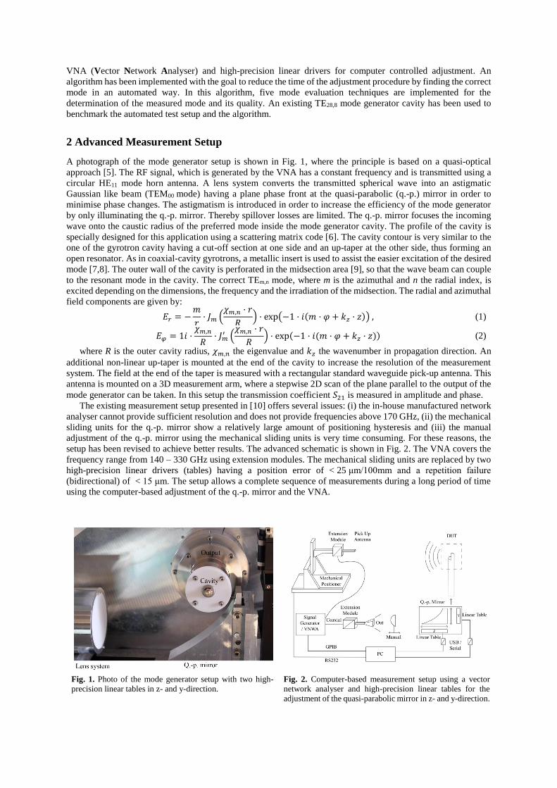
A photograph of the mode generator setup is shown in Fig. 1, where the principle is based on a quasi-optical
approach [5]. The RF signal, which is generated by the VNA has a constant frequency and is transmitted using a
circular HE11 mode horn antenna. A lens system converts the transmitted spherical wave into an astigmatic
Gaussian like beam (TEM00 mode) having a plane phase front at the quasi-parabolic (q.-p.) mirror in order to
minimise phase changes. The astigmatism is introduced in order to increase the efficiency of the mode generator
by only illuminating the q.-p. mirror. Thereby spillover losses are limited. The q.-p. mirror focuses the incoming
wave onto the caustic radius of the preferred mode inside the mode generator cavity. The profile of the cavity is
specially designed for this application using a scattering matrix code [6]. The cavity contour is very similar to the
one of the gyrotron cavity having a cut-off section at one side and an up-taper at the other side, thus forming an
open resonator. As in coaxial-cavity gyrotrons, a metallic insert is used to assist the easier excitation of the desired
mode [7,8]. The outer wall of the cavity is perforated in the midsection area [9], so that the wave beam can couple
to the resonant mode in the cavity. The correct TEm,n mode, where m is the azimuthal and n the radial index, is
excited depending on the dimensions, the frequency and the irradiation of the midsection. The radial and azimuthal
field components are given by:
𝐸𝑟 = −𝑚
𝑟· 𝐽𝑚 (
𝜒𝑚,𝑛 · 𝑟
𝑅) · exp(−1 · 𝑖(𝑚 · 𝜑 + 𝑘𝑧 · 𝑧)) , (1)
𝐸𝜑 = 1𝑖 ·𝜒𝑚,𝑛
𝑅· 𝐽𝑚
′ (𝜒𝑚,𝑛 · 𝑟
𝑅) · exp(−1 · 𝑖(𝑚 · 𝜑 + 𝑘𝑧 · 𝑧)) (2)
where R is the outer cavity radius, 𝜒𝑚,𝑛 the eigenvalue and 𝑘𝑧 the wavenumber in propagation direction. An
additional non-linear up-taper is mounted at the end of the cavity to increase the resolution of the measurement
system. The field at the end of the taper is measured with a rectangular standard waveguide pick-up antenna. This
antenna is mounted on a 3D measurement arm, where a stepwise 2D scan of the plane parallel to the output of the
mode generator can be taken. In this setup the transmission coefficient 𝑆21 is measured in amplitude and phase.
The existing measurement setup presented in [10] offers several issues: (i) the in-house manufactured network
analyser cannot provide sufficient resolution and does not provide frequencies above 170 GHz, (ii) the mechanical
sliding units for the q.-p. mirror show a relatively large amount of positioning hysteresis and (iii) the manual
adjustment of the q.-p. mirror using the mechanical sliding units is very time consuming. For these reasons, the
setup has been revised to achieve better results. The advanced schematic is shown in Fig. 2. The VNA covers the
frequency range from 140 – 330 GHz using extension modules. The mechanical sliding units are replaced by two
high-precision linear drivers (tables) having a position error of < 25 μm/100mm and a repetition failure
(bidirectional) of < 15 μm. The setup allows a complete sequence of measurements during a long period of time
using the computer-based adjustment of the q.-p. mirror and the VNA.
Fig. 1. Photo of the mode generator setup with two high-
precision linear tables in z- and y-direction.
Fig. 2. Computer-based measurement setup using a vector
network analyser and high-precision linear tables for the
adjustment of the quasi-parabolic mirror in z- and y-direction.

3 Intelligent Algorithms for Automatic Adjustment
The most challenging and time-consuming task is given by the excitation of the correct mode. To improve this
situation, the measurement procedure shown in Fig. 3 has been developed using an automated adjustment [11].
First of all, the transmitting horn antenna (Tx antenna), the lens system, the q.-p. mirror and the cavity is
implemented as a 2D model with MATLAB. The ideal distances between antenna and lens system, and q.-p. mirror
and cavity can be calculated and are used as a start position for the optimisation. In the next step of the procedure,
called ”Lens System Adjustment”, the calculated position for the lens system is proven by measurements. This step
cannot be done automatized because the lens system has to be disassembled from the setup. Using the ideal
simulation values, the distances are checked between antenna and lens system, and between lens system and
receiving (Rx) antenna, which is a placeholder for the q.-p. mirror. Through this measurement, a wave with only
a minimum phase change (plane wave) can be achieved at the plane where the q.-p. mirror is positioned.
In the next step, the lens system is assembled to the mode generator setup again and the operating frequency
of the designed cavity has to be determined. The transmission coefficient is plotted in Fig. 4 for a frequency sweep
from 138 – 142 GHz, where the Rx pick-up antenna is positioned on the field maximum of the desired mode.
There are three main maxima which indicate the frequencies of excited modes using a certain q.-p. mirror position.
These resonant frequencies are at 140.006, 138.07 and 140.85 GHz. The implemented algorithm searches for the
amplitude peak which is closest to the nominal frequency (here 140.0 GHz) in the first iteration.
The closest peak at 140.006 GHz is chosen for the next step “Find Correct Mirror Position”. A change of the
mirror position in an area of ≈ 5x5 mm around the ideal q.-p. mirror position, which is calculated using the already
mentioned MATLAB code, is performed where the Rx antenna is still positioned on the field maximum of the
desired mode. The q.-p. mirror is driven with a step size of 0.1 mm in the before mentioned 5x5 mm area in x- and
y-direction. The result of this procedure step can be seen in Fig. 5. The graph shows the amplitude in dependence
of the q.-p. mirror position. The mirror position with the highest amplitude value (here: x = 69.2 mm, y = 85.2 mm)
represents an adjustment which excites a mode with a high quality. This position can differ from the ideal position
due to fabrication tolerances and mirror rotation. A mode pattern with low resolution (pixel size: 0.5x0.5 mm) is
taken with the chosen q.-p. mirror position. The acquired mode pattern is evaluated using the mode evaluation
techniques presented in Ch. 4: Mode Evaluation Techniques where the excited TEm,n mode can be determined.
After a successful evaluation, the code can determine if the excited mode is the correct one or not and gives a
statement about its purity. If the excited mode seems to be not correct, the procedure does the second iteration by
searching the second peak in the frequency range from 138 – 142 GHz. But, if the correct mode is excited, the
mode pattern is measured with higher accuracies (pixel size: 0.2x0.2 mm). In the following, fine tuning can be
done. Therefore, mode patterns with high resolution are taken with a change of ± 0.1 - 0.2 mm in the x- and y-
direction of the q.-p. mirror to probably increase the purity of the excited mode. The launcher and the mirror system
can be verified after the successful excitation of the mode using this procedure.
Fig. 3. Measurement procedure for a time saving mode evaluation algorithm.
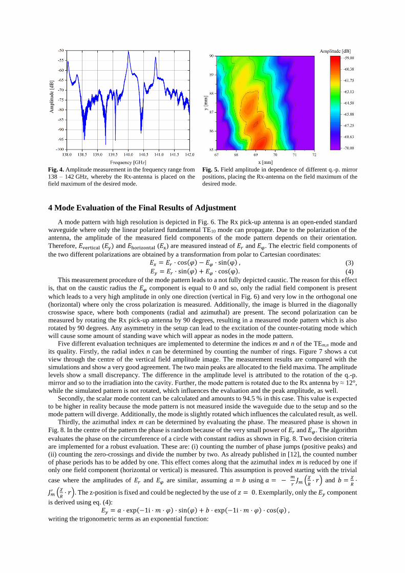
Fig. 4. Amplitude measurement in the frequency range from
138 – 142 GHz, whereby the Rx-antenna is placed on the
field maximum of the desired mode.
Fig. 5. Field amplitude in dependence of different q.-p. mirror
positions, placing the Rx-antenna on the field maximum of the
desired mode.
4 Mode Evaluation of the Final Results of Adjustment
A mode pattern with high resolution is depicted in Fig. 6. The Rx pick-up antenna is an open-ended standard
waveguide where only the linear polarized fundamental TE10 mode can propagate. Due to the polarization of the
antenna, the amplitude of the measured field components of the mode pattern depends on their orientation.
Therefore, 𝐸vertical (𝐸y) and 𝐸horizontal (𝐸x) are measured instead of 𝐸𝑟 and 𝐸φ. The electric field components of
the two different polarizations are obtained by a transformation from polar to Cartesian coordinates:
𝐸𝑥 = 𝐸𝑟 · cos(𝜑) − 𝐸𝜑 · sin(φ) , (3)
𝐸𝑦 = 𝐸𝑟 · sin(𝜑) + 𝐸𝜑 · cos(φ). (4)
This measurement procedure of the mode pattern leads to a not fully depicted caustic. The reason for this effect
is, that on the caustic radius the 𝐸𝜑 component is equal to 0 and so, only the radial field component is present
which leads to a very high amplitude in only one direction (vertical in Fig. 6) and very low in the orthogonal one
(horizontal) where only the cross polarization is measured. Additionally, the image is blurred in the diagonally
crosswise space, where both components (radial and azimuthal) are present. The second polarization can be
measured by rotating the Rx pick-up antenna by 90 degrees, resulting in a measured mode pattern which is also
rotated by 90 degrees. Any asymmetry in the setup can lead to the excitation of the counter-rotating mode which
will cause some amount of standing wave which will appear as nodes in the mode pattern.
Five different evaluation techniques are implemented to determine the indices m and n of the TEm,n mode and
its quality. Firstly, the radial index n can be determined by counting the number of rings. Figure 7 shows a cut
view through the centre of the vertical field amplitude image. The measurement results are compared with the
simulations and show a very good agreement. The two main peaks are allocated to the field maxima. The amplitude
levels show a small discrepancy. The difference in the amplitude level is attributed to the rotation of the q.-p.
mirror and so to the irradiation into the cavity. Further, the mode pattern is rotated due to the Rx antenna by ≈ 12°,
while the simulated pattern is not rotated, which influences the evaluation and the peak amplitude, as well.
Secondly, the scalar mode content can be calculated and amounts to 94.5 % in this case. This value is expected
to be higher in reality because the mode pattern is not measured inside the waveguide due to the setup and so the
mode pattern will diverge. Additionally, the mode is slightly rotated which influences the calculated result, as well.
Thirdly, the azimuthal index m can be determined by evaluating the phase. The measured phase is shown in
Fig. 8. In the centre of the pattern the phase is random because of the very small power of 𝐸𝑟 and 𝐸𝜑. The algorithm
evaluates the phase on the circumference of a circle with constant radius as shown in Fig. 8. Two decision criteria
are implemented for a robust evaluation. These are: (i) counting the number of phase jumps (positive peaks) and
(ii) counting the zero-crossings and divide the number by two. As already published in [12], the counted number
of phase periods has to be added by one. This effect comes along that the azimuthal index m is reduced by one if
only one field component (horizontal or vertical) is measured. This assumption is proved starting with the trivial
case where the amplitudes of 𝐸𝑟 and 𝐸𝜑 are similar, assuming 𝑎 = 𝑏 using 𝑎 = − 𝑚
𝑟𝐽𝑚 (
𝜒
𝑅· 𝑟) and 𝑏 =
𝜒
𝑅·
𝐽𝑚′ (
𝜒
𝑅· 𝑟). The z-position is fixed and could be neglected by the use of 𝑧 = 0. Exemplarily, only the 𝐸𝑦 component
is derived using eq. (4):
𝐸𝑦 = 𝑎 · exp(−1i · 𝑚 · 𝜑) · sin(𝜑) + 𝑏 · exp(−1i · 𝑚 · 𝜑) · cos(φ) ,
writing the trigonometric terms as an exponential function:

𝐸𝑦 = 𝑎 · exp(−1i · 𝑚 · 𝜑) ·exp(𝑖𝜑) − exp(−𝑖𝜑)
2+ 𝑎 · exp(−1i · 𝑚 · 𝜑) ·
exp(𝑖𝜑) + exp(−𝑖𝜑)
2 ,
𝐸𝑦 = 𝑎 · exp(−1i · 𝜑(𝑚 − 1)). (5)
The argument arg(𝐸𝑦) of eq. 5 is set to zero, whereby the number of zero crossings can be found.
arg(𝐸𝑦) =sin (−𝜑(𝑚 − 1))
cos(−𝜑(𝑚 − 1))= 0
𝜑 = 𝜋 · 𝑛
𝑚 − 1 , (6)
where 𝑛 ∈ ℤ. Equation 6 implies that the pattern has 2(𝑚 − 1) zero-crossings or 𝑚 − 1 phase jumps over a period
of 2𝜋. The non-trivial case (𝑎 ≠ 𝑏) can be solved assuming 𝑎
𝑚≤ 𝑏 ≤ 5𝑎 and −5𝑎 ≤ 𝑏 ≤ −
𝑎
𝑚 for 𝑎 < 0, where
eq. 6 is valid, as well. The evaluation on the circle is most robust if the evaluation radius is slightly smaller than
the caustic radius. Figure 9 shows the 2D plot of the unwrapped phase on the circumference of the circle. The
phase difference between the measured phase and a linear fitted one is evaluated. This phase difference shows a
rotation of ≈ 12°, which can be seen in the amplitude mode pattern in Fig. 6, as well. The areas around -102°
(ideally -90°) and +78° (ideally +90°) are highlighted and marks the section where only the 𝐸𝑟 component is
measured. The phase difference is increased or respectively decreased in the greyed area. In this area the amplitude
of the radial 𝐸𝑟 component is decreasing and the amplitude of the azimuthal 𝐸𝜑 component is increasing. The
phase change in this area is because of the mixture of 𝐸𝑟 and 𝐸𝜑, which have a 90° phase shift to each other, as
presented in eq. (1) and (2).
The fourth mode evaluation technique concerns to the amount of the counter-rotating mode. The complete
suppression of the counter-rotating mode is not possible due to the unsymmetrical principle of the excitation. The
amount of the counter-rotating mode is an important number to verify the quality of the mode generator and is
defined by the power ratio between the unwanted counter-rotating (-) mode and the wanted co-rotating (+) mode.
The formula is given by [13]:
𝑝−
𝑝+= (
Δ𝐸 − 1
Δ𝐸 + 1)
2
(7)
with
Δ𝐸 = 10𝐸max/dB−𝐸min/dB
20 , where 𝐸max and 𝐸min are described by the maximal and minimal measured field amplitudes along the first
azimuthal ring in the mode pattern and 𝑝+ and 𝑝− are related to the relative power fractions of the co- and counter-
rotating mode. The counter-rotating amount is calculated to be 0.33 %, which indicates a good cavity design and
adjustment of the system. The algorithm used for the phase evaluation is applied with only small modifications in
this evaluation method, as well.
Fifthly, the measured quality factor of the cavity can be compared with the simulated one. The measured
quality factor is determined from Fig. 4 by 𝑄 = 𝑓res/𝐵3 dB = 2548 and is in good agreement with the designed
cavity quality factor of 2533.
Fig. 6. Measured amplitude pattern of the TE28,8 mode
operating at 140.006 GHz.
Fig. 7. Vertical cut of the amplitude mode picture from the
TE28,8 mode measurement and simulation.

Fig. 8. Measured phase of the TE28,8 mode operating at
140.006 GHz.
Fig. 9. Unwrapped phase from the measured TE28,8 mode
pattern on the circumference of a constant radius compared
with a linear fitted phase. The difference phase is calculated
by subtracting the measured and linear phase.
5 Repeatability Test for TE28,10 mode generator cavity
For a 1.5 MW gyrotron which is under discussion for upgrading the existing 1 MW TE28,8 mode gyrotrons for W7-
X (Wendelstein 7-X [14]) the TE28,10 mode operating at 140 GHz has been selected as a suitable cavity mode [15].
A TE28,10 mode generator cavity has been fabricated and tested using both mode generator test setups. In this study
a time saving of a factor 10 and additionally higher mode purity has been achieved. In Figs. 10 and 11 the measured
amplitude and phase pattern are plotted. The measured mode is confirmed to be the TE28,10 mode operating at
140.01 GHz using the given mode evaluation techniques. The algorithms calculated that the scalar mode content
is 93 %, the counter-rotating amount is 0.57 % and the quality factor is 2522, which is in good agreement with the
simulated quality factor of 2506.
Fig. 10. Measured amplitude pattern of the TE28,10 mode
operating at 140.006 GHz.
Fig. 11. Measured phase pattern of the TE28,10 mode
operating at 140.006 GHz.
6 Summary and Outlook
In this paper, the automatized adjustment of a gyrotron mode generator for cold tests is shown to provide the
excitation of very high order rotating modes in waveguides with a high mode purity. The old test setup has been
modified installing a VNA, high precision linear drivers and 3D measurement arm which are controlled via
computer. Therefore, higher position and measurement accuracies are achieved. The computer-based controlling
allows a positioning which is independent of human attendance. Five mode evaluation techniques are implemented
determining the azimuthal and radial mode index, the scalar mode content, the amount of the counter-rotating
mode and the quality factor. The algorithm is able to efficiently detect, whether the measured mode pattern matches
with the given theoretical mode or not. The newly designed and presented measurement system is benchmarked

using an existing TE28,8 mode cavity operating at 140.006 GHz achieving a mode purity of approximately 95 %
and a counter-rotating amount of only around 0.4 %. The repeatability of the procedure was successfully
demonstrated for a TE28,10 mode cavity, where an adjustment time saving of a factor of approximately 10 was
achieved.
References
1. A. Sawant, et al., Scientific Reports, vol. 7, no.: 3372 (2017)
2. T. Omori, et al., Fusion Eng. Des., vol. 86, pp. 951-954, 2011.
3. T. Rzesnicki, et al., Trans. On Plasma Science, vol. 38, no. 6, pp. 1141-1149, 2010.
4. T. Ruess, et al., EPJ Web Conf., vol. 187 (2018).
5. N. Aleksandrov, et al., Int. J. Infrared and Millimeter Waves, 13, 1369-1385, 1992.
6. D. Wagner, et al., Int. J. Infrared and Millimeter Waves 19,185-194 (1998).
7. C. T. Iatrou, et al., IEEE Trans. Microwave Theory Tech., vol. 44, pp. 56-64, 1996.
8. K. A. Avramides, et al., IEEE Trans. on Plasma Science, vol. 32, no. 3, 2004.
9. M. Pereyaslavets, et al., Int. J. Electronics, 82:1, pp. 107-115, 1997.
10. M. Losert, J. Jin and T. Rzesnicki, in IEEE Trans. on Plasma Science, vol. 41, no. 3, pp. 628-632, March
2013.
11. T. Ruess, et al., EPJ Web Conf., (2018).
12. M. Losert, et al., 2015 German Microwave Conference, Nuernberg, 2015, pp. 256-259.
13. A. Arnold, G. Dammertz and M. Thumm, IRMMW, Conference Digest of the 2004 Joint 29th International
Conference on 2004 and 12th International Conference on Terahertz Electronics, 2004., 2004, pp. 671-672.
14. H. Braune, et al, in Proc. IRMMW, Copenhagen, Denmark, Sep. 2016, pp. 1-2.
15. K. A. Avramidis, et al., 20th Joint Workshop on Electron Cyclotron Emission (ECE) and Electron Cyclotron
Resonance Heating (ECRH), May 2018, Greifswald, Germany.


