AMV investigation
Document NWPSAF-MO-TR-028
Version 0.4
04/10/13
Comparing AMVs over the Indian Ocean James Cotton Met Office, UK
Comparing AMVs over the Indian Ocean
Doc ID : NWPSAF-MO-TR-028 Version : 0.4 Date : 04/10/13
Comparing AMVs over the Indian Ocean
James Cotton Met Office, UK
This documentation was developed within the context of the EUMETSAT Satellite Application Facility on Numerical Weather Prediction (NWP SAF), under the Cooperation Agreement dated 29 June 2011, between EUMETSAT and the Met Office, UK, by one or more partners within the NWP SAF. The partners in the NWP SAF are the Met Office, ECMWF, KNMI and Météo France. Copyright 2013, EUMETSAT, All Rights Reserved.
Change record Version Date Author / changed by Remarks
0.1 04/04/13 J Cotton First draft 0.2 15/07/13 J Cotton Add section with trial results 0.3 18/07/13 J Cotton First version for review 0.4 04/10/13 J Cotton Minor updates following comments from J.
Eyre and P. Francis.
1
Contents
1 Introduction ....................................... .....................................................................2
2 AMVs from IODC satellites .......................... ..........................................................3
2.1 Overview of Meteosat-7, FY-2D/E and Kalpana ................................................3
2.2 Data coverage...................................................................................................5
2.3 Data volume......................................................................................................6
2.4 Timeliness.........................................................................................................6
3 CGMS statistics.................................... ..................................................................7
3.1 IR winds ............................................................................................................8
3.2 WV winds..........................................................................................................8
3.3 Summary...........................................................................................................9
4 Long-term trends ................................... ..............................................................12
5 NWP SAF plots ...................................... ...............................................................16
5.1 January 2013 ..................................................................................................16
5.2 July 2012.........................................................................................................23
6 Statistics versus QI ............................... ...............................................................26
7 Quality control and assigned errors ................ ...................................................27
8 Assimilation experiments ........................... .........................................................29
9 Conclusions........................................ ..................................................................34
References......................................... ..........................................................................36
Appendix – CMA derivation changes.................. .......................................................36
2
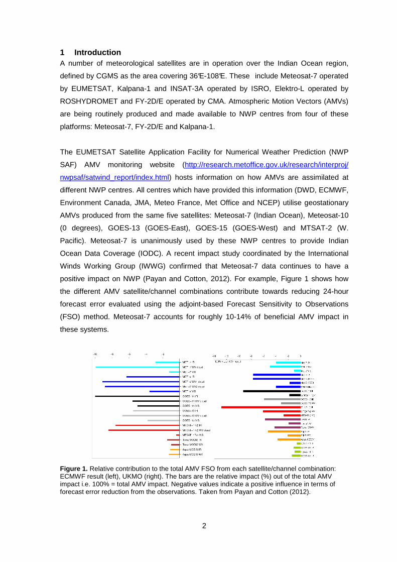
1 Introduction A number of meteorological satellites are in operation over the Indian Ocean region,
defined by CGMS as the area covering 36°E-108°E. These include Meteosat-7 operated
by EUMETSAT, Kalpana-1 and INSAT-3A operated by ISRO, Elektro-L operated by
ROSHYDROMET and FY-2D/E operated by CMA. Atmospheric Motion Vectors (AMVs)
are being routinely produced and made available to NWP centres from four of these
platforms: Meteosat-7, FY-2D/E and Kalpana-1.
The EUMETSAT Satellite Application Facility for Numerical Weather Prediction (NWP
SAF) AMV monitoring website (http://research.metoffice.gov.uk/research/interproj/
nwpsaf/satwind_report/index.html) hosts information on how AMVs are assimilated at
different NWP centres. All centres which have provided this information (DWD, ECMWF,
Environment Canada, JMA, Meteo France, Met Office and NCEP) utilise geostationary
AMVs produced from the same five satellites: Meteosat-7 (Indian Ocean), Meteosat-10
(0 degrees), GOES-13 (GOES-East), GOES-15 (GOES-West) and MTSAT-2 (W.
Pacific). Meteosat-7 is unanimously used by these NWP centres to provide Indian
Ocean Data Coverage (IODC). A recent impact study coordinated by the International
Winds Working Group (IWWG) confirmed that Meteosat-7 data continues to have a
positive impact on NWP (Payan and Cotton, 2012). For example, Figure 1 shows how
the different AMV satellite/channel combinations contribute towards reducing 24-hour
forecast error evaluated using the adjoint-based Forecast Sensitivity to Observations
(FSO) method. Meteosat-7 accounts for roughly 10-14% of beneficial AMV impact in
these systems.
Figure 1. Relative contribution to the total AMV FSO from each satellite/channel combination: ECMWF result (left), UKMO (right). The bars are the relative impact (%) out of the total AMV impact i.e. 100% = total AMV impact. Negative values indicate a positive influence in terms of forecast error reduction from the observations. Taken from Payan and Cotton (2012).
3
The provision of the Meteosat IODC service is not a primary mission of EUMETSAT.
Instead this mission is a ‘best-efforts’ undertaking which makes use of a residual
Meteosat First Generation (MFG) capacity to bridge a (temporary) gap in data coverage.
Whilst a residual MSG capacity (e.g. Meteosat-8) may become available following
commissioning of MSG-4 in around mid-2015, the extension of MFG remains the only
agreed approach to continue the IODC mission. Given the uncertainties in the long-term
provision of IODC, the purpose of this investigation is to re-evaluate the current
alternatives to Meteosat-7 from China and India. AMV products from Meteosat-7, FY-
2D/E and Kalpana-1 are the subject of this inter-comparison study
2 AMVs from IODC satellites
2.1 Overview of Meteosat-7, FY-2D/E and Kalpana An overview of the main satellite and AMV characteristics for each of the IODC satellites
is presented in Table 1.
Meteosat-7 FY-2D FY-2E Kalpana-1 Location 57.5E 86.5E 105E 74E Launch 1997
(IODC from 2006) 2006 2008 2002
Operator EUMETSAT CMA CMA ISRO Imager channels
IR (11.3 µm) VIS (0.7 µm) WV (6.3 µm)
IR (10.8 µm) IR12 (12.0 µm) SWIR (3.8 µm) VIS (0.7µm) WV (6.8 µm)
IR (10.8 µm) IR12 (12.0 µm) SWIR (3.8 µm) VIS (0.7µm) WV (6.8 µm)
IR (11.5 µm) VIS (0.65 µm) WV (6.4 µm)
Pixel Resolution at SSP
5.0 km: IR, WV 2.5 km: VIS
5.0 km IR, WV 1.25 km VIS
5.0 km IR, WV 1.25 km VIS
8km: IR, WV 2km: VIS
AMVs IR, VIS, WV, CSWV
IR, Mixed WV IR, Mixed WV IR, Mixed WV
AMV target size
32x32: IR, CSWV 16x16: WV, VIS
Full disk cycle
Every 30 mins Every 30 mins Every 30 mins Every 30 mins
AMV temporal resolution
1.5 hr
6 hr 03,09,15,21 UTC
6 hr 00,06,12,18 UTC
3 hr
AMV coverage (approx)
4W-118E 60S-60N
32E-142E 54S-54N
50E-160E 52S-52N
22E-128E 48S-49N
Table 1. General characteristics of Meteosat-7, FY-2D, FY-2E and Kalpana. IR = infrared, SWIR = shortwave IR, WV = cloudy water vapour, CSWV = clear-sky water vapour, VIS = visible.
4
Meteosat-7 is the last remaining platform of the Meteosat First Generation Programme
and has been stationed over the Indian Ocean since its relocation in December 2006. It
carries the Meteosat Visible Infra-Red Imager (MVIRI): a 3-channel imager covering the
infrared (IR), visible (VIS) and water-vapour (WV) bands. Pixel resolution is 5 km for IR
and WV and 2.5 km for VIS and full disk images are available every 30 mins. AMVs are
derived every 90 mins and quality indicators (QI) are provided following the standard
EUMETSAT methodology. For more information on the Meteosat-7 AMV derivation see
Schmetz et al. (1993).
FY-2D and FY-2E are the current operational geostationary satellites operated by the
Chinese Meteorological Agency (CMA) and carry a 5-channel imager. Full disk images
are produced every 30 mins and AMVs are currently extracted in the IR and WV
channels at 5 km pixel resolution. CMA provide the clear-sky and cloudy WV winds in
one product. However it would be more useful if they were available separately as
geostationary clear-sky WV winds are usually of poorer quality. AMVs are derived every
6 hours and FY-2D winds are offset by 3 hours relative to FY-2E with the aim of
obtaining 3-hourly winds for the overlap areas of 2D and 2E. However, the 3 hour shift
away from standard synoptic times means it is not possible to compare FY2D winds with
radiosonde data. FY-2D is less well-calibrated, images are known to be affected by
stray-light and the spectral response of the WV channel is not well-defined. The FY-2F
satellite was launched in January 2012 but for the time-being CMA plan to use 2F for
rapid scanning for severe weather. It is not yet clear when FY-2F may replace FY-2E
(with FY-2E to replace FY-2D).
Kalpana-1 is the first geostationary meteorological satellite developed and operated by
the Indian Space Research Organisation (ISRO). It carries a 3-channel imager with 8 km
pixel resolution for IR/WV and 2 km for VIS. Full disk images are available every 30 mins
and IR and WV AMVs are derived every 3 hours. Like CMA, ISRO also provide the
clear-sky and cloudy WV winds in one product. Until May 2013, height assignment has
been based on the Genetic Algorithm (GA): an empirical method that tries to reproduce
Meteosat-7 heights without the use of an NWP background. An improved AMV
derivation scheme presented at the recent International Winds Workshop (see Deb et
al., 2012) has recently been implemented operationally (31 May 2013) but has yet to be
stored at the Met Office due to corrections in the BUFR format. As such the Kalpana
data discussed in this report are from the old GA algorithm. A complication with the
Indian winds is that Kalpana winds are generated at India Meteorological Department
(IMD) using software provided by the research team at ISRO which can lead to delays in
5
the implementation of changes. AMV products from the alternative INSAT satellite series
have yet to be made operational. The latest satellite, INSAT-3D, is due to be launched in
2013 and will carry a GOES-type imager.
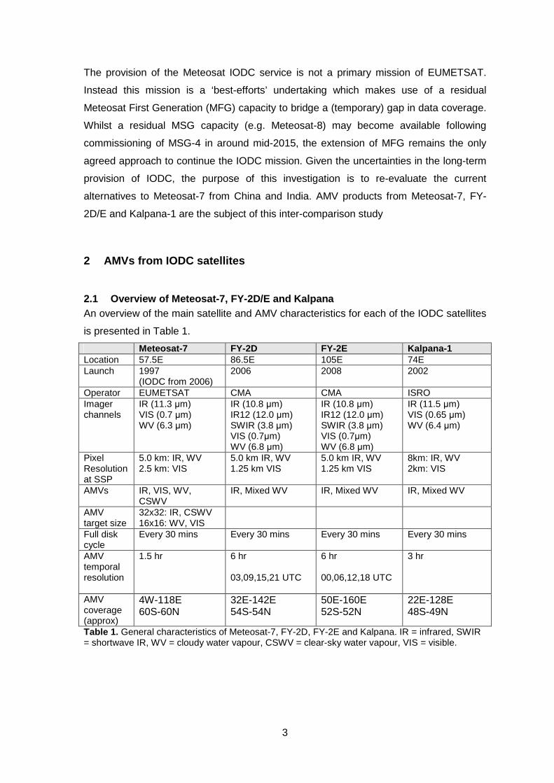
2.2 Data coverage Plots showing the spatial coverage of AMVs from the different satellites are given in
Figure 2. Kalpana lies over the centre of the Indian Ocean region and is closest to the
position of Meteosat-7. However, the square-shaped coverage area of Kalpana extends
to only around 49°N/S compared to 60°N/S for Meteosat -7. FY-2D and FY-2E are
separated by only 19 degrees and so have a large overlap region but are much further
east than Meteosat-7. FY-2E (the better satellite) is located in the ‘primary’ CMA position
at 105°E which unfortunately covers less of the Indian O cean region than FY-2D.
Meteosat-9 is able to cover the far west of the basin but use of FY2-E alone for IODC
would result in data gaps in the mid-latitudes. FY-2D has a slightly larger latitudinal
coverage at 54°N/S but both are short of Meteosat-7.
Figure 2. Data coverage plots for a 6-hour period centred at 12 UTC on 15 January 2013: Meteosat-7 (top left), FY-2D/E (top right) and Kalpana-1 (bottom left) AMVs. Meteosat-9 is also shown compared with FY-2E as this extends into the far west of the Indian Ocean (bottom right).
6
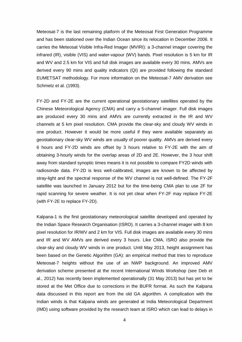
2.3 Data volume Figure 3 compares the data volume of the EUMETSAT and CMA winds during January
2013. Data volumes are around 25% and 100% higher for Meteosat-7 IR and WV
channels respectively compared to FY-2E. There are substantially fewer WV winds from
FY-2D and FY-2E despite the inclusion of the clear sky targets in the mixed WV product
(Met-7 cloudy WV only). The number of IR winds is more similar, especially considering
the Meteosat-7 winds are produced 4x more frequently.
Figure 3. Number of Meteosat-7, FY-2D and FY-2E win ds during January 2013: IR (left) and WV (right). Data has been filtered for QI2 > 80. Th e dropout from 18-20 January was due to monitoring job failures and is unrelated to the dat a supply.
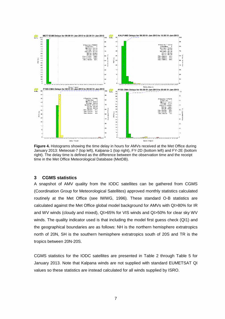
2.4 Timeliness An important consideration for use of new data products in operational NWP is the
timeliness in which the observations are received. The NWP SAF monitoring website
(http://research.metoffice.gov.uk/research/interproj/nwpsaf/satwind_report/index.html)
hosts information on the time requirements for several NWP centres. In general it is
desirable that data are received as soon as possible. Figure 4 compares the timeliness
of Meteosat-7, Kalpana-1 and FY-2D/E observations received from EUMETSAT, ISRO
and CMA respectively during January 2013. Nearly all data from Meteosat-7, Kalpana-1
and FY-2E were received in less than 3 hours, meaning a significant amount of data
would have been available for use in assimilation. FY-2D was less timely with only 40%
of data arriving in less than 3 hours and only 4% arriving in time for the main forecast
run. Meteosat-7 data was the timeliest with a mean delay of just over 30 minutes. Data
availability throughout January 2013 was good from EUMETSAT and CMA but the winds
received from ISRO were patchier with missing time slots on around 2 out of every 3
days.
7
Figure 4. Histograms showing the time delay in hours for AMVs received at the Met Office during January 2013: Meteosat-7 (top left), Kalpana-1 (top right), FY-2D (bottom left) and FY-2E (bottom right). The delay time is defined as the difference between the observation time and the receipt time in the Met Office Meteorological Database (MetDB).
3 CGMS statistics A snapshot of AMV quality from the IODC satellites can be gathered from CGMS
(Coordination Group for Meteorological Satellites) approved monthly statistics calculated
routinely at the Met Office (see IWWG, 1996). These standard O-B statistics are
calculated against the Met Office global model background for AMVs with QI>80% for IR
and WV winds (cloudy and mixed), QI>65% for VIS winds and QI>50% for clear sky WV
winds. The quality indicator used is that including the model first guess check (QI1) and
the geographical boundaries are as follows: NH is the northern hemisphere extratropics
north of 20N, SH is the southern hemisphere extratropics south of 20S and TR is the
tropics between 20N-20S.
CGMS statistics for the IODC satellites are presented in Table 2 through Table 5 for
January 2013. Note that Kalpana winds are not supplied with standard EUMETSAT QI
values so these statistics are instead calculated for all winds supplied by ISRO.
8
3.1 IR winds At high level (above 400 hPa) the Meteosat-7 IR winds show a strong dependence on
latitude. In the extratropics the winds exhibit a significant negative wind speed bias of
nearly 3 m/s and increased levels of RMSVD. The slow speed bias is slightly worse in
the northern hemisphere and is linked to the increase in observed wind speed. In the
tropics, where there are a large number of winds, data quality is good. At mid level (400-
700 hPa) the IR winds are generally poorer in quality but tempered by the fact fewer
winds are derived here. The tropical winds at mid level exhibit a positive speed bias of
around 2 m/s. At low level (below 700 hPa) the observed wind speed is much lower and
the AMVs are generally of good quality with neutral wind speed bias and low levels of
RMSVD. The exception is for a very small number of winds extracted in the NH.
As there is a high degree of overlap between the coverage of FY-2D and FY-2E the two
CMA platforms can be compared more directly. In general the O-B statistics for the two
satellites are broadly similar. At high level, the negative speed bias is around 5 m/s in
the northern hemisphere and RMSVD values are high at over 9 m/s. In the tropics
however, there are a large number of good quality winds and the RMS vector differences
are slightly better by around 0.5 m/s for FY-2E compared to FY-2D. The statistics at mid
level follow a similar pattern. The number of winds extracted at low level is comparably
low for both satellites. Rather unusually, for FY-2D there are more winds at mid level
than there are at low level. Outside the northern hemisphere, the quality of the low level
winds is reasonable with RMSVD values of 3.5 m/s in the tropics.
The Kalpana winds are generally of poor quality with high RMS vector differences
observed at all levels. In comparison to Meteosat-7 and FY-2D/E, there are an unusually
high number of winds assigned to mid level.
3.2 WV winds The Meteosat-7 WV winds are extracted from tracking cloudy targets only and so
virtually all winds are located at high level. In the extratropics the negative speed bias of
around 1 m/s is significantly smaller in magnitude than that seen for the IR winds.
However the tropical WV winds have more of a positive speed bias and higher RMSVD
compared to the IR.
The WV winds from FY-2D and FY-2E are a derived from tracking a mixture of clear and
cloudy targets and so are located across a much larger depth of the troposphere. The
9
statistics show that in general the FY-2E WV winds are of a much higher quality than
FY-2D with RMS vector differences around 0.5-2.0 m/s lower for FY-2E. This is likely
due to known issues with the FY-2D WV channel (spectral response not well
characterised). It is also noticeable that the WV winds show smaller departures
compared to the IR winds. For example, at high and mid level the negative speed bias
in the extratropics is only around 1-2 m/s for FY-2E WV winds versus around 3-6 m/s for
the IR winds. In general the FY-2E WV winds appear to be of good quality at mid-high
level.
Departures for the Kalpana mixed WV winds are large and variable.
3.3 Summary Although not a direct like-for-like comparison due to the differences in geographical
coverage, the statistics can still offer a broad relative comparison between the platforms
for January 2013. The Meteosat-7 IR AMVs are of slightly higher quality than the IR
winds from FY-2D and FY-2E. In particular, the negative speed bias in the northern
hemisphere appears more pronounced in the data from CMA. This is despite the fact
that Meteosat-7 data captures a higher mean wind speed. Generally in the tropics, the
statistics from Meteosat-7 and FY-2D/E are very comparable and at mid level the CMA
data doesn’t exhibit the positive speed bias seen in the EUMETSAT data. Further
investigation would be needed to ascertain whether this is due to geographical
differences.
Interpreting the differences in the WV winds is not straightforward due to the fact the
CMA winds are also tracking clear-sky targets. At high level, the negative speed bias in
the northern hemisphere is again slightly worse for FY-2E compared to Met-7. However,
in the topics and southern hemisphere the high level statistics from FY-2E are more
favourable. At mid level the number of winds from FY-2E is a factor of 10 greater due to
the additional tracking of clear-sky targets and RMS vector differences here are smaller
than seen from Meteosat-7.
Kalpana AMVs making use of the old GA algorithm are generally of poor quality and so
will not be considered any further in this study.
10
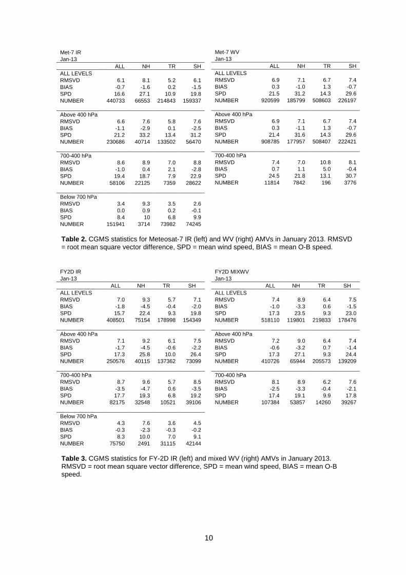
Met-7 IR Jan-13 ALL NH TR SH ALL LEVELS RMSVD 6.1 8.1 5.2 6.1 BIAS -0.7 -1.6 0.2 -1.5 SPD 16.6 27.1 10.9 19.8 NUMBER 440733 66553 214843 159337 Above 400 hPa RMSVD 6.6 7.6 5.8 7.6 BIAS -1.1 -2.9 0.1 -2.5 SPD 21.2 33.2 13.4 31.2 NUMBER 230686 40714 133502 56470 700-400 hPa RMSVD 8.6 8.9 7.0 8.8 BIAS -1.0 0.4 2.1 -2.8 SPD 19.4 18.7 7.9 22.9 NUMBER 58106 22125 7359 28622 Below 700 hPa RMSVD 3.4 9.3 3.5 2.6 BIAS 0.0 0.9 0.2 -0.1 SPD 8.4 10 6.8 9.9 NUMBER 151941 3714 73982 74245 Table 2. CGMS statistics for Meteosat-7 IR (left) and WV (right) AMVs in January 2013. RMSVD = root mean square vector difference, SPD = mean wind speed, BIAS = mean O-B speed. FY2D IR Jan-13 ALL NH TR SH ALL LEVELS RMSVD 7.0 9.3 5.7 7.1 BIAS -1.8 -4.5 -0.4 -2.0 SPD 15.7 22.4 9.3 19.8 NUMBER 408501 75154 178998 154349 Above 400 hPa RMSVD 7.1 9.2 6.1 7.5 BIAS -1.7 -4.5 -0.6 -2.2 SPD 17.3 25.8 10.0 26.4 NUMBER 250576 40115 137362 73099 700-400 hPa RMSVD 8.7 9.6 5.7 8.5 BIAS -3.5 -4.7 0.6 -3.5 SPD 17.7 19.3 6.8 19.2 NUMBER 82175 32548 10521 39106 Below 700 hPa RMSVD 4.3 7.6 3.6 4.5 BIAS -0.3 -2.3 -0.3 -0.2 SPD 8.3 10.0 7.0 9.1 NUMBER 75750 2491 31115 42144 Table 3. CGMS statistics for FY-2D IR (left) and mixed WV (right) AMVs in January 2013. RMSVD = root mean square vector difference, SPD = mean wind speed, BIAS = mean O-B speed.
Met-7 WV Jan-13 ALL NH TR SH ALL LEVELS RMSVD 6.9 7.1 6.7 7.4 BIAS 0.3 -1.0 1.3 -0.7 SPD 21.5 31.2 14.3 29.6 NUMBER 920599 185799 508603 226197 Above 400 hPa RMSVD 6.9 7.1 6.7 7.4 BIAS 0.3 -1.1 1.3 -0.7 SPD 21.4 31.6 14.3 29.6 NUMBER 908785 177957 508407 222421 700-400 hPa RMSVD 7.4 7.0 10.8 8.1 BIAS 0.7 1.1 5.0 -0.4 SPD 24.5 21.8 13.1 30.7 NUMBER 11814 7842 196 3776
FY2D MIXWV Jan-13 ALL NH TR SH ALL LEVELS RMSVD 7.4 8.9 6.4 7.5 BIAS -1.0 -3.3 0.6 -1.5 SPD 17.3 23.5 9.3 23.0 NUMBER 518110 119801 219833 178476 Above 400 hPa RMSVD 7.2 9.0 6.4 7.4 BIAS -0.6 -3.2 0.7 -1.4 SPD 17.3 27.1 9.3 24.4 NUMBER 410726 65944 205573 139209 700-400 hPa RMSVD 8.1 8.9 6.2 7.6 BIAS -2.5 -3.3 -0.4 -2.1 SPD 17.4 19.1 9.9 17.8 NUMBER 107384 53857 14260 39267
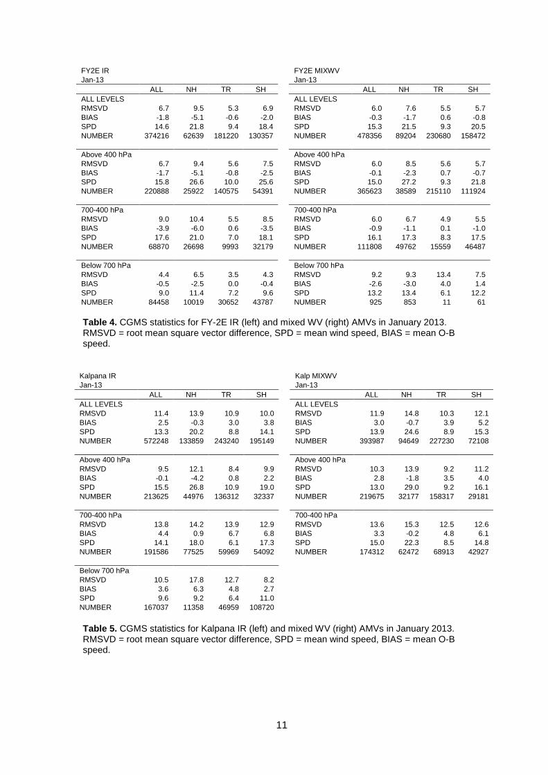
11
FY2E IR FY2E MIXWV Jan-13 Jan-13 ALL NH TR SH ALL NH TR SH ALL LEVELS ALL LEVELS RMSVD 6.7 9.5 5.3 6.9 RMSVD 6.0 7.6 5.5 5.7 BIAS -1.8 -5.1 -0.6 -2.0 BIAS -0.3 -1.7 0.6 -0.8 SPD 14.6 21.8 9.4 18.4 SPD 15.3 21.5 9.3 20.5 NUMBER 374216 62639 181220 130357 NUMBER 478356 89204 230680 158472 Above 400 hPa Above 400 hPa RMSVD 6.7 9.4 5.6 7.5 RMSVD 6.0 8.5 5.6 5.7 BIAS -1.7 -5.1 -0.8 -2.5 BIAS -0.1 -2.3 0.7 -0.7 SPD 15.8 26.6 10.0 25.6 SPD 15.0 27.2 9.3 21.8 NUMBER 220888 25922 140575 54391 NUMBER 365623 38589 215110 111924 700-400 hPa 700-400 hPa RMSVD 9.0 10.4 5.5 8.5 RMSVD 6.0 6.7 4.9 5.5 BIAS -3.9 -6.0 0.6 -3.5 BIAS -0.9 -1.1 0.1 -1.0 SPD 17.6 21.0 7.0 18.1 SPD 16.1 17.3 8.3 17.5 NUMBER 68870 26698 9993 32179 NUMBER 111808 49762 15559 46487 Below 700 hPa Below 700 hPa RMSVD 4.4 6.5 3.5 4.3 RMSVD 9.2 9.3 13.4 7.5 BIAS -0.5 -2.5 0.0 -0.4 BIAS -2.6 -3.0 4.0 1.4 SPD 9.0 11.4 7.2 9.6 SPD 13.2 13.4 6.1 12.2 NUMBER 84458 10019 30652 43787 NUMBER 925 853 11 61 Table 4. CGMS statistics for FY-2E IR (left) and mixed WV (right) AMVs in January 2013. RMSVD = root mean square vector difference, SPD = mean wind speed, BIAS = mean O-B speed.
Kalpana IR Kalp MIXWV Jan-13 Jan-13 ALL NH TR SH ALL NH TR SH ALL LEVELS ALL LEVELS RMSVD 11.4 13.9 10.9 10.0 RMSVD 11.9 14.8 10.3 12.1 BIAS 2.5 -0.3 3.0 3.8 BIAS 3.0 -0.7 3.9 5.2 SPD 13.3 20.2 8.8 14.1 SPD 13.9 24.6 8.9 15.3 NUMBER 572248 133859 243240 195149 NUMBER 393987 94649 227230 72108 Above 400 hPa Above 400 hPa RMSVD 9.5 12.1 8.4 9.9 RMSVD 10.3 13.9 9.2 11.2 BIAS -0.1 -4.2 0.8 2.2 BIAS 2.8 -1.8 3.5 4.0 SPD 15.5 26.8 10.9 19.0 SPD 13.0 29.0 9.2 16.1 NUMBER 213625 44976 136312 32337 NUMBER 219675 32177 158317 29181 700-400 hPa 700-400 hPa RMSVD 13.8 14.2 13.9 12.9 RMSVD 13.6 15.3 12.5 12.6 BIAS 4.4 0.9 6.7 6.8 BIAS 3.3 -0.2 4.8 6.1 SPD 14.1 18.0 6.1 17.3 SPD 15.0 22.3 8.5 14.8 NUMBER 191586 77525 59969 54092 NUMBER 174312 62472 68913 42927 Below 700 hPa RMSVD 10.5 17.8 12.7 8.2 BIAS 3.6 6.3 4.8 2.7 SPD 9.6 9.2 6.4 11.0 NUMBER 167037 11358 46959 108720
Table 5. CGMS statistics for Kalpana IR (left) and mixed WV (right) AMVs in January 2013. RMSVD = root mean square vector difference, SPD = mean wind speed, BIAS = mean O-B speed.
12
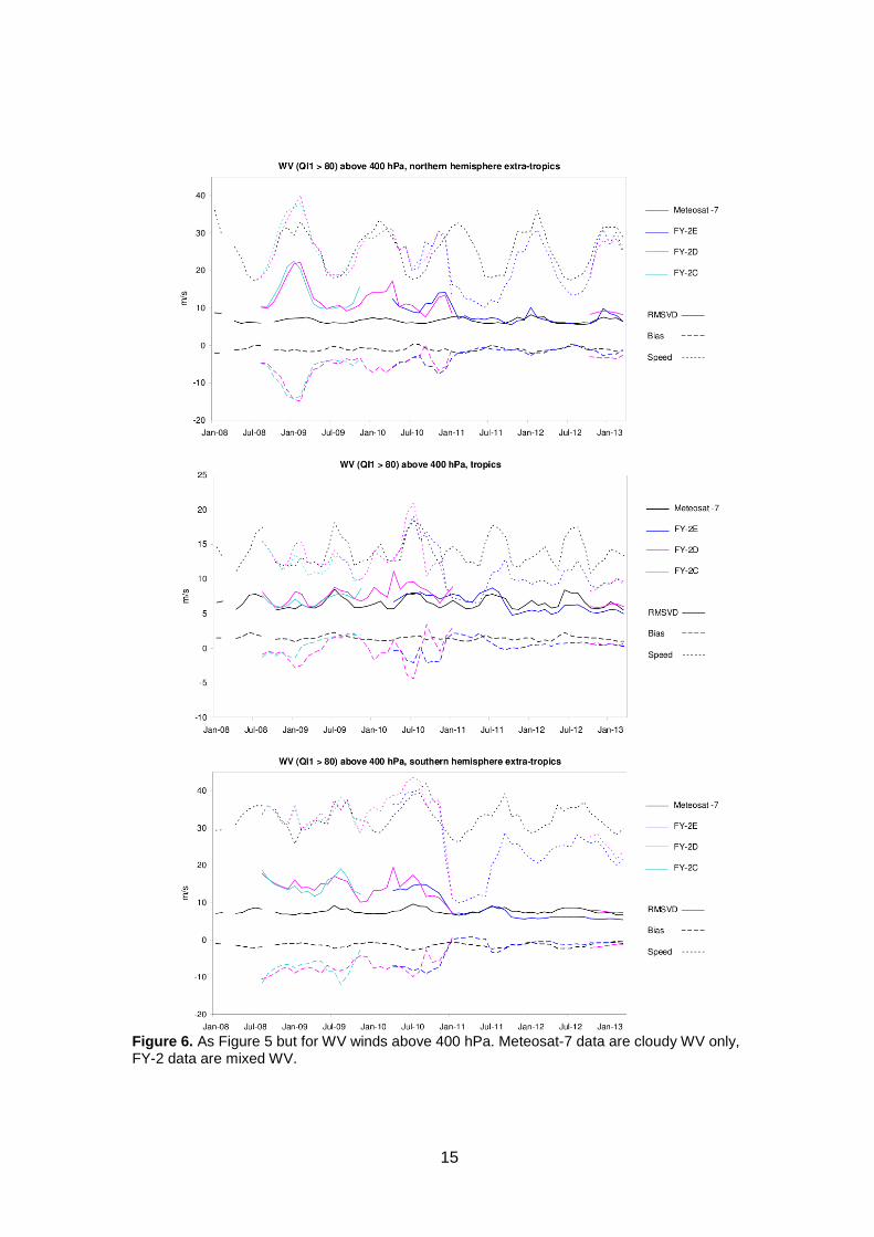
4 Long-term trends Met Office CGMS statistics accumulated from the past several years can be used to
investigate seasonal and long term trends in AMV quality. The stability of the products is
an important factor to consider for NWP.
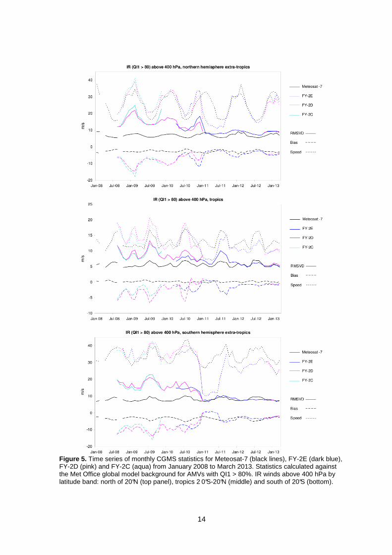
Figure 5 to Figure 7 show the variation in RMSVD, mean O-B speed bias and mean
observed speed from January 2008 until March 2013 for data from Meteosat-7 and FY2-
C/D/E. It is clear from the CGMS statistics that whilst the Meteosat-7 data has remained
very stable over the past 5 years, there have been significant changes in the data
characteristics from CMA. There have been three (known) major derivation changes
made by CMA during this time: late 2009, January 2011 and September 2011.
Information on the changes as supplied by CMA is available in the Appendix.
The impact on the CMA data can be clearly seen in Figure 5 which shows IR winds at
high level. If we first consider the northern hemisphere (top plot) then we see that
through 2008 and 2009, FY2-C and FY-2D both exhibit a large and variable seasonal
bias. For FY-2D, the negative speed bias and RMSVD peak at -15 m/s and 22 m/s
respectively and clearly coincides with the peak in wind speed in northern hemisphere
winter. After the first CMA update in late 2009 we lose data from FY-2C, but for FY-2D
we can observe that the peak in bias/RMSVD in January 2010 is reduced compared to
levels of February 2009. From April 2010 the Met Office began monitoring data from FY-
2E and initially the data quality appears slightly worse than FY-2D. Following the CMA
update in January 2011 we notice several changes: 1) loss of data from FY-2D, 2) sharp
reduction in RMSVD and speed bias, 3) sharp drop in the mean observed wind speed.
These are largely the result of changes to the QI characteristics as, after the update,
there are very few AMVs with high observed wind speeds that have QI1 > 80. For FY-2D
it was found that all winds had a QI value of 50 and therefore no data at all remained
above the monitoring threshold. From September 2011 the faster AMVs are once again
retained with no obvious impact on wind vector quality. RMSVD and bias levels are
closer to Meteosat-7 but are still slightly higher for FY-2E. More recently, FY-2D has
reappeared from October 2012 onwards and also note the dip in observed wind speed in
January 2013.
A similar pattern of changes can be observed in the southern hemisphere but with a few
small differences (bottom panel of Figure 5). Following the September 2011 change the
southern hemisphere AMVs from FY-2E appear much closer in quality to Meteosat-7
and in fact have a lower RMSVD and bias from around April-November 2012. In the
13
most recent months, data quality from all three satellites appears similar, although
observed wind speeds from FY-2D/E remain lower.
The plot of high level IR data in the tropics also tells a similar story of gradual
improvement in AMV quality from CMA (middle panel of Figure 5). Note the change in
scale of the wind speed axis from the extratropics.
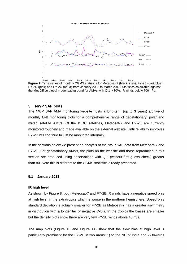
Figure 7 shows that the low level IR winds are generally now quite similar in quality. The
mean wind speed bias from Meteosat-7 is around a few tenths of m/s above zero, whilst
the mean bias from FY-2D/E is around a few tenths of m/s below zero.
If we consider just the WV (cloudy for Meteosat-7, mixed for FY2) winds at high level as
shown in Figure 6 then we observe a similar pattern of changes to that of the IR. For the
northern hemisphere (top panel), the CMA winds at the start of 2009 again have a large
bias coinciding with the winter months. From a peak in bias and RMSVD of -15 m/s and
22 m/s respectively (same as IR) in February 2009, a gradual trend towards a reduction
in peak levels of bias can be seen for the following two winters up to January 2011.
Following the changes in 2011, FY-2E data quality appears much more stable and
similar to that of Meteosat-7. Although the mean observed wind speed recovered
following the September 2011 change it still remains several m/s lower than Meteosat-7.
In the southern hemisphere and tropics (bottom and middle panels of Figure 6), the
mixed WV winds from FY-2E actually have lower RMSVD values than Meteosat-7
following the September 2011 change.
The high level FY-2E WV winds are of a higher quality than FY-2D. There are two
reasons why we might expect AMVs in general from FY-2D to be of lower quality (ref
CMA, October 2011):
1. The image calibration of FY-2D is worse than FY-2E
2. The time schedule of FY-2D at 03,09,15,21 UTC (3 hour departures from FY-2E)
means than it is not possible to compare with radiosonde data. Algorithm
changes are therefore prepared and tested with FY-2E and then directly applied
to FY-2D.
The results presented here show that only the WV winds are inferior for FY-2D so this
probably due to the known issues with the FY-2D WV channel spectral response
function.
14
Figure 5. Time series of monthly CGMS statistics for Meteosat-7 (black lines), FY-2E (dark blue), FY-2D (pink) and FY-2C (aqua) from January 2008 to March 2013. Statistics calculated against the Met Office global model background for AMVs with QI1 > 80%. IR winds above 400 hPa by latitude band: north of 20°N (top panel), tropics 2 0°S-20°N (middle) and south of 20°S (bottom).
15
Figure 6. As Figure 5 but for WV winds above 400 hPa. Meteosat-7 data are cloudy WV only, FY-2 data are mixed WV.
16
Figure 7. Time series of monthly CGMS statistics for Meteosat-7 (black lines), FY-2E (dark blue), FY-2D (pink) and FY-2C (aqua) from January 2008 to March 2013. Statistics calculated against the Met Office global model background for AMVs with QI1 > 80%. IR winds below 700 hPa.
5 NWP SAF plots The NWP SAF AMV monitoring website hosts a long-term (up to 3 years) archive of
monthly O-B monitoring plots for a comprehensive range of geostationary, polar and
mixed satellite AMVs. Of the IODC satellites, Meteosat-7 and FY-2E are currently
monitored routinely and made available on the external website. Until reliability improves
FY-2D will continue to just be monitored internally.
In the sections below we present an analysis of the NWP SAF data from Meteosat-7 and
FY-2E. For geostationary AMVs, the plots on the website and those reproduced in this
section are produced using observations with QI2 (without first-guess check) greater
than 80. Note this is different to the CGMS statistics already presented.
5.1 January 2013
IR high level
As shown by Figure 8, both Meteosat-7 and FY-2E IR winds have a negative speed bias
at high level in the extratropics which is worse in the northern hemisphere. Speed bias
standard deviation is actually smaller for FY-2E as Meteosat-7 has a greater asymmetry
in distribution with a longer tail of negative O-B's. In the tropics the biases are smaller
but the density plots show there are very few FY-2E winds above 40 m/s.
The map plots (Figure 10 and Figure 11) show that the slow bias at high level is
particularly prominent for the FY-2E in two areas: 1) to the NE of India and 2) towards
17
the East China Sea and Japan. As FY-2E lies slightly further east than FY-2D it is likely
to cover more of the slow bias region near Japan. This may explain why in the CGMS
statistics FY-2E has a larger speed bias in northern hemisphere than FY-2D. The slow
bias near Japan coincides with the (peak) fast winds of the strong upper level jet stream
as captured by the model. The slow bias to the NE of India appears not to be associated
with the jet stream but instead occurs over the very high terrain north of the Himalayas
and over Western China.
IR mid level
At mid level (not shown) the IR speed bias statistics are generally poor in the
extratropics. The CMA winds show a larger negative speed bias but Meteosat-7 shows
greater variation and poorer correlation.
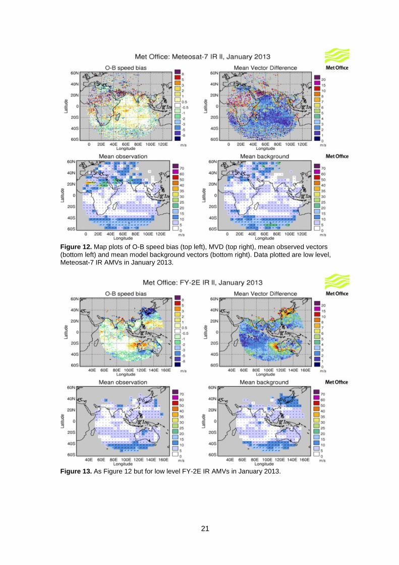
IR low level
For low level IR data (Figure 9) Meteosat-7 shows some spuriously fast winds,
particularly in the tropics and northern hemisphere where there is a marked asymmetry.
The CMA winds in the northern hemisphere also show poorer statistics and continue to
show a negative speed bias. In the tropics the CMA winds are less biased than
Meteosat-7. In the southern hemisphere Meteosat-7 has a neutral wind speed bias and
lower O-B standard deviation than FY-2E.
The FY-2E low level map (Figure 13) shows that northern hemisphere negative speed
bias for the CMA winds is localised to a region near Korea/Japan. The vector plots show
that this bias is the result of observations not properly capturing the strength of winds
flowing off the Asian continent (winter monsoon). Mean vector differences are also quite
high off the West coast of Australia. The Meteosat-7 winds over sea are mostly unbiased
(Figure 12). Over land however, many of the winds show a significant fast bias,
particularly north of the equator over Africa, the Arabian Peninsula and Northern India.
This bias coincides with the position of the upper level jet (Figure 10) and is indicative of
a large height assignment error in these cases.
WV high level
The speed bias characteristics of the high level WV winds are similar to that described
for the IR. The main difference is that the negative speed bias for the CMA winds is
reduced for the mixed WV winds compared to the IR. Outside the northern hemisphere,
mean speed bias and vector differences are low for FY-2E and clearly lower than
Meteosat-7 in the overlap region (Figure 14).
18
Zonal plots
The high-mid level slow bias is the dominant feature of the FY-2E IR zonal plot (Figure
15). The CMA winds also have a slow bias at very high level (above 150 hPa) in the
tropics. Meteosat-7 IR has strong biases located around 500-600 hPa: a slow bias near
40S and a fast bias near 20N. The FY-2E WV winds are derived much deeper in the
troposphere and are assigned to more discrete height bands below about 350 hPa. The
fast bias for Meteosat-7 WV winds extends from around 20°N to 40°S.
19
Figure 8. Density plots of observation versus model background wind speed for Meteosat-7 (top panel) and FY-2E (bottom) IR AMVs above 400 hPa. Statistics are calculated by latitude band against the Met Office global model background for January 2013.
Figure 9. As per Figure 8 but for IR AMVs below 700 hPa.
20
Figure 10. Map plots of O-B speed bias (top left), MVD (top right), mean observed vectors (bottom left) and mean model background vectors (bottom right). Data plotted are high level, Meteosat-7 IR AMVs in January 2013.
Figure 11. As Figure 10 but for high level FY-2E IR AMVs in January 2013.
21
Figure 12. Map plots of O-B speed bias (top left), MVD (top right), mean observed vectors (bottom left) and mean model background vectors (bottom right). Data plotted are low level, Meteosat-7 IR AMVs in January 2013.
Figure 13. As Figure 12 but for low level FY-2E IR AMVs in January 2013.
22
Figure 14. Map plots of O-B speed bias (left) and MVD (right). Data plotted are high level, Meteosat-7 WV (top) and FY-2E mixed WV (bottom) AMVs in January 2013.
Met Office: Meteosat-7, IR (left) and WV (right), January 2013
Met Office: FY-2E, IR (left) and mixed WV (right), January 2013
Figure 15. Zonal plots of O-B speed bias for Meteosat-7 (top) and FY-2E (bottom) for IR (left) and WV (right) AMVs in January 2013.
23
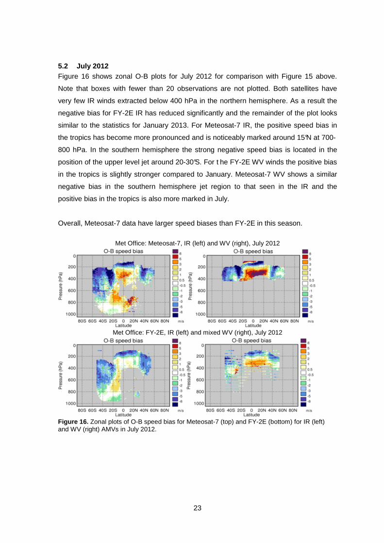
5.2 July 2012 Figure 16 shows zonal O-B plots for July 2012 for comparison with Figure 15 above.
Note that boxes with fewer than 20 observations are not plotted. Both satellites have
very few IR winds extracted below 400 hPa in the northern hemisphere. As a result the
negative bias for FY-2E IR has reduced significantly and the remainder of the plot looks
similar to the statistics for January 2013. For Meteosat-7 IR, the positive speed bias in
the tropics has become more pronounced and is noticeably marked around 15°N at 700-
800 hPa. In the southern hemisphere the strong negative speed bias is located in the
position of the upper level jet around 20-30°S. For t he FY-2E WV winds the positive bias
in the tropics is slightly stronger compared to January. Meteosat-7 WV shows a similar
negative bias in the southern hemisphere jet region to that seen in the IR and the
positive bias in the tropics is also more marked in July.
Overall, Meteosat-7 data have larger speed biases than FY-2E in this season.
Met Office: Meteosat-7, IR (left) and WV (right), July 2012
Met Office: FY-2E, IR (left) and mixed WV (right), July 2012
Figure 16. Zonal plots of O-B speed bias for Meteosat-7 (top) and FY-2E (bottom) for IR (left) and WV (right) AMVs in July 2012.
24
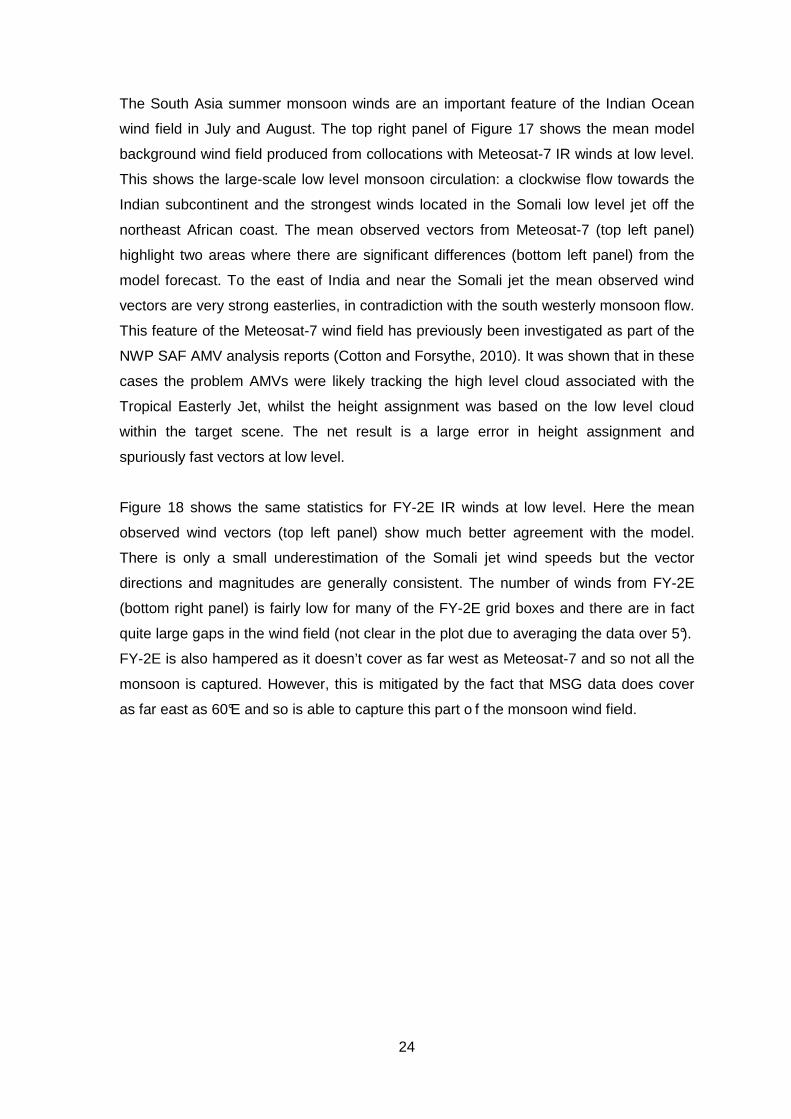
The South Asia summer monsoon winds are an important feature of the Indian Ocean
wind field in July and August. The top right panel of Figure 17 shows the mean model
background wind field produced from collocations with Meteosat-7 IR winds at low level.
This shows the large-scale low level monsoon circulation: a clockwise flow towards the
Indian subcontinent and the strongest winds located in the Somali low level jet off the
northeast African coast. The mean observed vectors from Meteosat-7 (top left panel)
highlight two areas where there are significant differences (bottom left panel) from the
model forecast. To the east of India and near the Somali jet the mean observed wind
vectors are very strong easterlies, in contradiction with the south westerly monsoon flow.
This feature of the Meteosat-7 wind field has previously been investigated as part of the
NWP SAF AMV analysis reports (Cotton and Forsythe, 2010). It was shown that in these
cases the problem AMVs were likely tracking the high level cloud associated with the
Tropical Easterly Jet, whilst the height assignment was based on the low level cloud
within the target scene. The net result is a large error in height assignment and
spuriously fast vectors at low level.
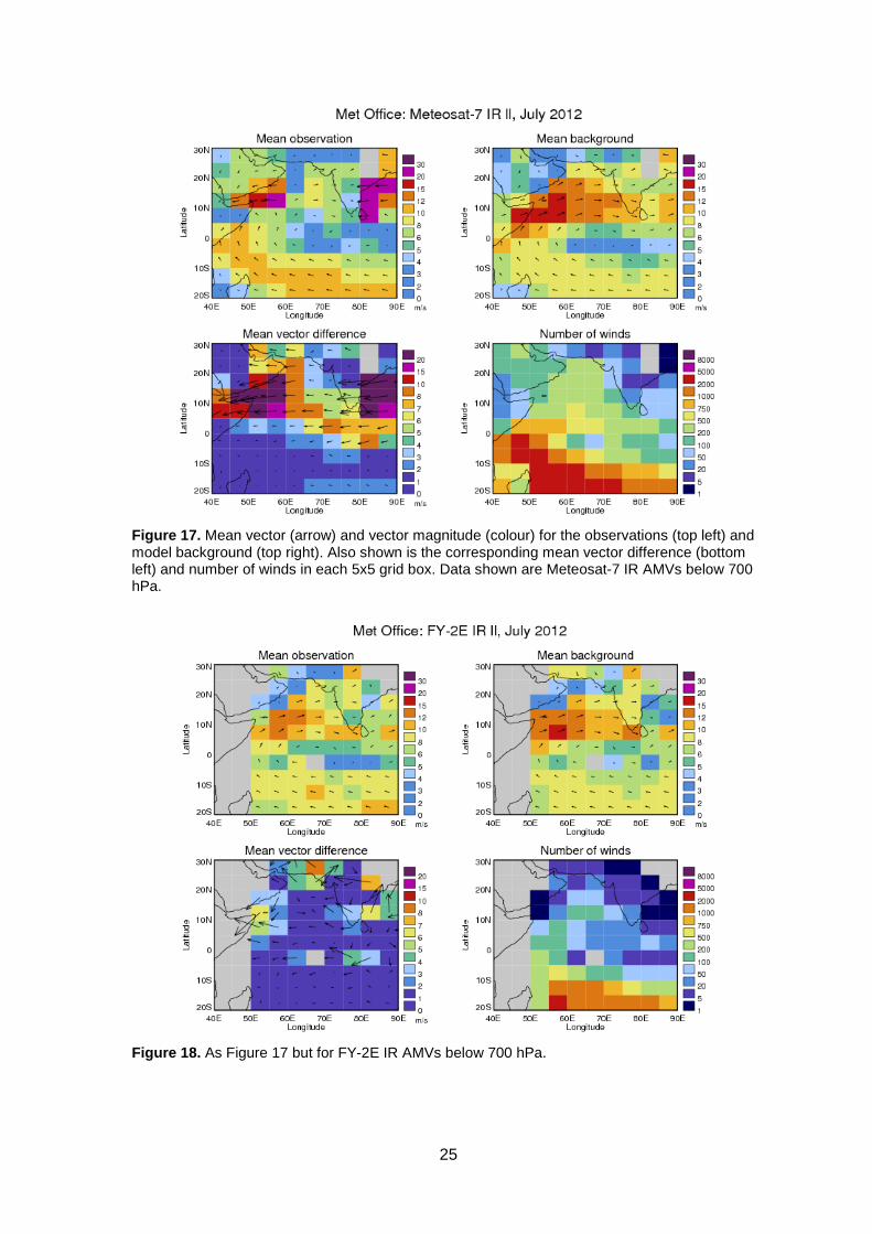
Figure 18 shows the same statistics for FY-2E IR winds at low level. Here the mean
observed wind vectors (top left panel) show much better agreement with the model.
There is only a small underestimation of the Somali jet wind speeds but the vector
directions and magnitudes are generally consistent. The number of winds from FY-2E
(bottom right panel) is fairly low for many of the FY-2E grid boxes and there are in fact
quite large gaps in the wind field (not clear in the plot due to averaging the data over 5°).
FY-2E is also hampered as it doesn’t cover as far west as Meteosat-7 and so not all the
monsoon is captured. However, this is mitigated by the fact that MSG data does cover
as far east as 60°E and so is able to capture this part o f the monsoon wind field.
25
Figure 17. Mean vector (arrow) and vector magnitude (colour) for the observations (top left) and model background (top right). Also shown is the corresponding mean vector difference (bottom left) and number of winds in each 5x5 grid box. Data shown are Meteosat-7 IR AMVs below 700 hPa.
Figure 18. As Figure 17 but for FY-2E IR AMVs below 700 hPa.
26
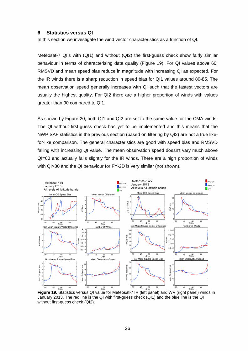
6 Statistics versus QI In this section we investigate the wind vector characteristics as a function of QI.
Meteosat-7 QI’s with (QI1) and without (QI2) the first-guess check show fairly similar
behaviour in terms of characterising data quality (Figure 19). For QI values above 60,
RMSVD and mean speed bias reduce in magnitude with increasing QI as expected. For
the IR winds there is a sharp reduction in speed bias for QI1 values around 80-85. The
mean observation speed generally increases with QI such that the fastest vectors are
usually the highest quality. For QI2 there are a higher proportion of winds with values
greater than 90 compared to QI1.
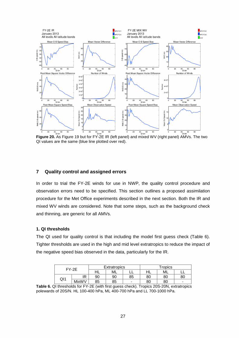
As shown by Figure 20, both QI1 and QI2 are set to the same value for the CMA winds.
The QI without first-guess check has yet to be implemented and this means that the
NWP SAF statistics in the previous section (based on filtering by QI2) are not a true like-
for-like comparison. The general characteristics are good with speed bias and RMSVD
falling with increasing QI value. The mean observation speed doesn't vary much above
QI=60 and actually falls slightly for the IR winds. There are a high proportion of winds
with QI>80 and the QI behaviour for FY-2D is very similar (not shown).
Figure 19. Statistics versus QI value for Meteosat-7 IR (left panel) and WV (right panel) winds in January 2013. The red line is the QI with first-guess check (QI1) and the blue line is the QI without first-guess check (QI2).
27
Figure 20. As Figure 19 but for FY-2E IR (left panel) and mixed WV (right panel) AMVs. The two QI values are the same (blue line plotted over red).
7 Quality control and assigned errors In order to trial the FY-2E winds for use in NWP, the quality control procedure and
observation errors need to be specified. This section outlines a proposed assimilation
procedure for the Met Office experiments described in the next section. Both the IR and
mixed WV winds are considered. Note that some steps, such as the background check
and thinning, are generic for all AMVs.
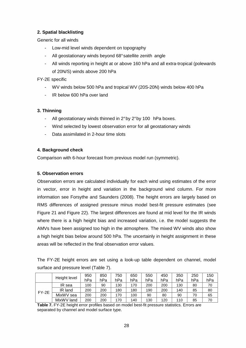
1. QI thresholds
The QI used for quality control is that including the model first guess check (Table 6).
Tighter thresholds are used in the high and mid level extratropics to reduce the impact of
the negative speed bias observed in the data, particularly for the IR.
Extratropics Tropics FY-2E
HL ML LL HL ML LL IR 90 90 85 80 80 80
QI1 MixWV 85 85 - 80 80 -
Table 6. QI thresholds for FY-2E (with first guess check). Tropics 20S-20N, extratropics polewards of 20S/N. HL 100-400 hPa, ML 400-700 hPa and LL 700-1000 hPa.
28
2. Spatial blacklisting
Generic for all winds
- Low-mid level winds dependent on topography
- All geostationary winds beyond 68° satellite zenith angle
- All winds reporting in height at or above 160 hPa and all extra-tropical (polewards
of 20N/S) winds above 200 hPa
FY-2E specific
- WV winds below 500 hPa and tropical WV (20S-20N) winds below 400 hPa
- IR below 600 hPa over land
3. Thinning
- All geostationary winds thinned in 2° by 2° by 100 hPa boxes.
- Wind selected by lowest observation error for all geostationary winds
- Data assimilated in 2-hour time slots
4. Background check
Comparison with 6-hour forecast from previous model run (symmetric).
5. Observation errors
Observation errors are calculated individually for each wind using estimates of the error
in vector, error in height and variation in the background wind column. For more
information see Forsythe and Saunders (2008). The height errors are largely based on
RMS differences of assigned pressure minus model best-fit pressure estimates (see
Figure 21 and Figure 22). The largest differences are found at mid level for the IR winds
where there is a high height bias and increased variation, i.e. the model suggests the
AMVs have been assigned too high in the atmosphere. The mixed WV winds also show
a high height bias below around 500 hPa. The uncertainly in height assignment in these
areas will be reflected in the final observation error values.
The FY-2E height errors are set using a look-up table dependent on channel, model
surface and pressure level (Table 7).
Height level 950 hPa
850 hPa
750 hPa
650 hPa
550 hPa
450 hPa
350 hPa
250 hPa
150 hPa
IR sea 100 90 130 170 200 200 130 80 70 IR land 200 200 180 180 190 200 140 85 80
MixWV sea 200 200 170 100 90 80 90 70 65 FY-2E
MixWV land 200 200 170 140 130 120 110 85 70 Table 7. FY-2E height error profiles based on model best-fit pressure statistics. Errors are separated by channel and model surface type.
29
Figure 21. Model best-fit pressure statistics for IR FY-2E winds in January 2013, separated by model surface type (land/sea). Left panels show the mean pressure difference (assigned minus best-fit) with one standard deviation error bars. Right panels show the RMS pressure difference in black. The red points just show the code default pressure errors and can be ignored.
Figure 22. As Figure 21 but for mixed WV FY-2E winds.
8 Assimilation experiments To compare the impact of AMVs from Meteosat-7 and FY-2E a set of assimilation
experiments were performed for the period 1 February 2013 to 25 March 2013, giving 52
days of verification. The experiment configurations were based on Parallel Suite 31
(PS31): the operational suite from January 2013. To save on computational resources
the horizontal forecast resolution was reduced to N320 (from N512) which equates to
approximately 40 km at mid-latitudes. The vertical grid dimensions were as per
operations with 70 vertical levels. Global analyses were created four times each day at
30
0, 6, 12 and 18 UTC using 4D-Var and forecasts were run at 0 and 12 UTC out to a lead
time of six days. A control suite (sjftb) was run with data-use closely matching that in
operations at the time, but with no AMVs over the Indian Ocean region. Experiments
sjcna and sjfte were then designed to measure (separately) the impact of adding the
Meteosat-7 and FY-2E winds respectively. For experiment sjcna the Meteosat-7 IR,
visible and cloudy WV winds were used as per the current operational configuration (see
NWP SAF website for details). For experiment sjfte the FY-2E IR and mixed WV winds
were used as outlined in the previous section.
An important metric for accessing forecast impact at the Met Office is the global NWP
index which is a weighted skill score combining improvements in forecast skill for a
number of atmospheric parameters. Note that the NWP index was substantially updated
in 2012 to give a more equal weight across lead times and some of the observations
used to verify each parameter have been revised. The change in forecast RMS
(experiment-control) for the NWP index parameters is given in Figure 23. The overall
distribution of impact looks rather similar. Both Meteosat-7 and FY-2E result in a small
negative impact of -0.20 points (~0.2%) when verified against quality controlled
observations. In the northern hemisphere the change in RMS is almost identical for the
two satellites with a negative impact on mean sea level pressure (PMSL) but a neutral-
positive impact on 500 hPa geopotential height and winds at 250 hPa. In the tropics both
have a positive impact on upper level winds, but Meteosat-7 has a better impact on the
low level 850 hPa winds compared to FY-2E. It is in the southern hemisphere where
most of the forecast degradation occurs with all three index parameters showing a
consistent increase in RMS. Winds at 250 hPa in particular are degraded. The negative
impact appears slightly worse for Meteosat-7 as the poorest verification for FY-2E (RMS
increase greater than 0.5%) is mainly limited to the longer forecast ranges.
The NWP index is representative of a small subset of forecast parameters but a wider
picture of forecast impact can seen by comparing plots of the full ‘extended’ index as in
Figure 24. Now the impact looks more favourable for Meteosat-7 in the northern
hemisphere and tropics with an overall small positive impact. Improvements are
observed for forecasts of temperature at 250 hPa (tropics and NH) and winds at 100
hPa. The impact of FY-2E appears more neutral in these regions, but there are still
improvements for high level temperature scores at 100 hPa and 250 hPa. The southern
hemisphere is where the differences between the two satellites are most prominent.
Both satellites have a clear negative impact on PMSL, wind and geopotential height
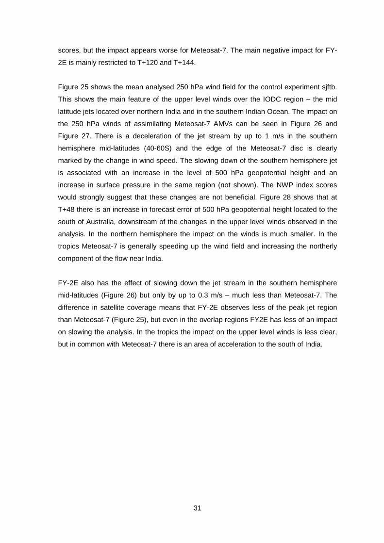
31
scores, but the impact appears worse for Meteosat-7. The main negative impact for FY-
2E is mainly restricted to T+120 and T+144.
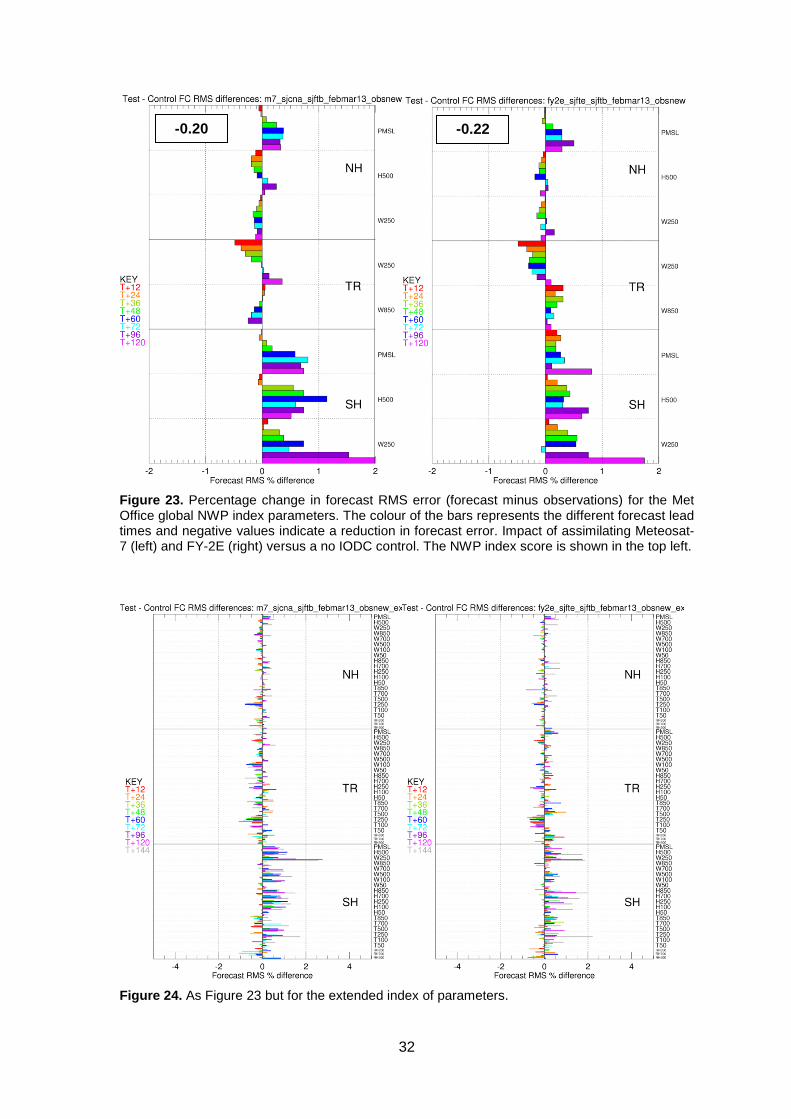
Figure 25 shows the mean analysed 250 hPa wind field for the control experiment sjftb.
This shows the main feature of the upper level winds over the IODC region – the mid
latitude jets located over northern India and in the southern Indian Ocean. The impact on
the 250 hPa winds of assimilating Meteosat-7 AMVs can be seen in Figure 26 and
Figure 27. There is a deceleration of the jet stream by up to 1 m/s in the southern
hemisphere mid-latitudes (40-60S) and the edge of the Meteosat-7 disc is clearly
marked by the change in wind speed. The slowing down of the southern hemisphere jet
is associated with an increase in the level of 500 hPa geopotential height and an
increase in surface pressure in the same region (not shown). The NWP index scores
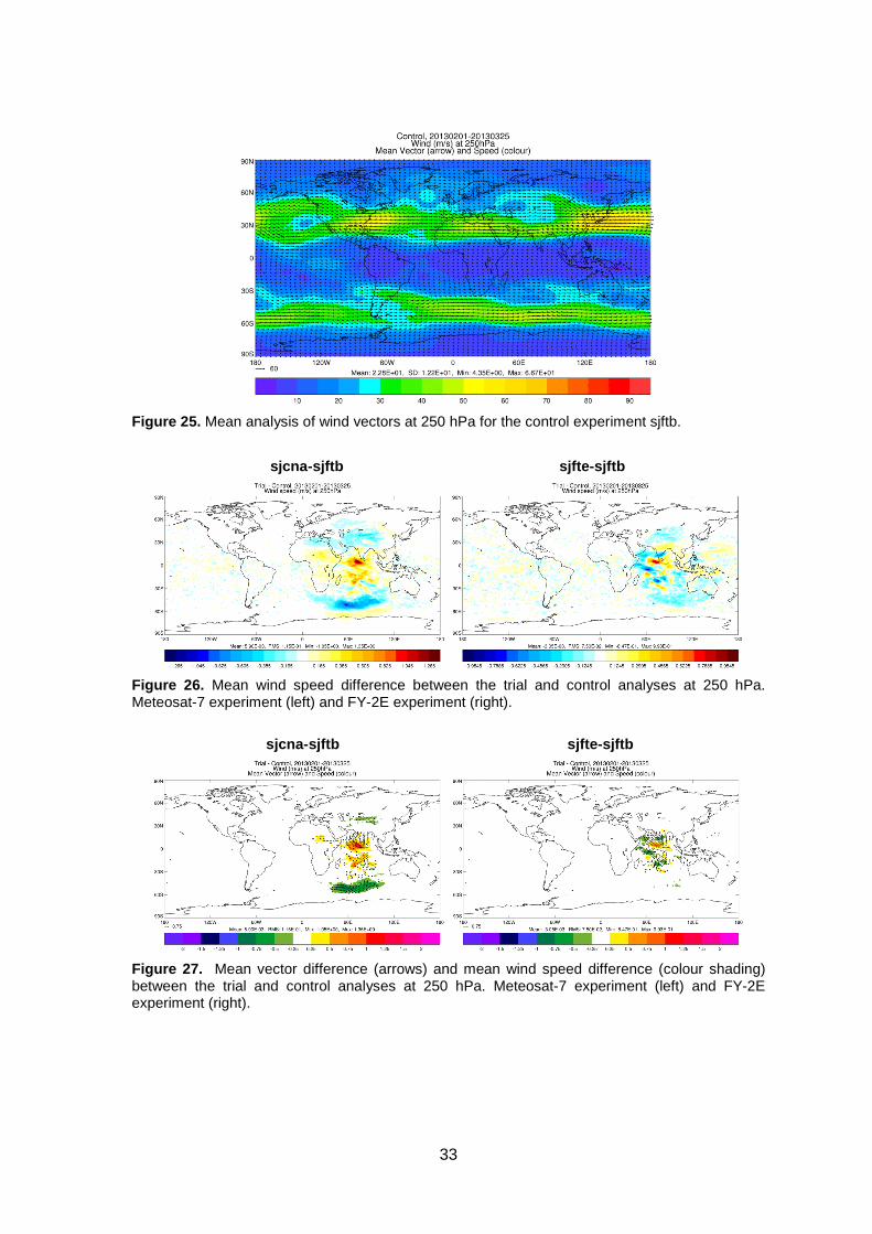
would strongly suggest that these changes are not beneficial. Figure 28 shows that at
T+48 there is an increase in forecast error of 500 hPa geopotential height located to the
south of Australia, downstream of the changes in the upper level winds observed in the
analysis. In the northern hemisphere the impact on the winds is much smaller. In the
tropics Meteosat-7 is generally speeding up the wind field and increasing the northerly
component of the flow near India.
FY-2E also has the effect of slowing down the jet stream in the southern hemisphere
mid-latitudes (Figure 26) but only by up to 0.3 m/s – much less than Meteosat-7. The
difference in satellite coverage means that FY-2E observes less of the peak jet region
than Meteosat-7 (Figure 25), but even in the overlap regions FY2E has less of an impact
on slowing the analysis. In the tropics the impact on the upper level winds is less clear,
but in common with Meteosat-7 there is an area of acceleration to the south of India.
32
Figure 23. Percentage change in forecast RMS error (forecast minus observations) for the Met Office global NWP index parameters. The colour of the bars represents the different forecast lead times and negative values indicate a reduction in forecast error. Impact of assimilating Meteosat-7 (left) and FY-2E (right) versus a no IODC control. The NWP index score is shown in the top left.
Figure 24. As Figure 23 but for the extended index of parameters.
-0.20 -0.22
33
Figure 25. Mean analysis of wind vectors at 250 hPa for the control experiment sjftb.
sjcna-sjftb sjft e-sjftb
Figure 26. Mean wind speed difference between the trial and control analyses at 250 hPa. Meteosat-7 experiment (left) and FY-2E experiment (right).
sjcna-sjftb sj fte-sjftb
Figure 27. Mean vector difference (arrows) and mean wind speed difference (colour shading) between the trial and control analyses at 250 hPa. Meteosat-7 experiment (left) and FY-2E experiment (right).
34
sjcna-sjftb sjf te-sjftb
Figure 28. Change in RMS error of forecasts of 500 hPa geopotential height at a lead time of 48 hours. Meteosat-7 experiment (left) and FY-2E experiment (right).
9 Conclusions Meteosat-7 is the prime satellite for the provision of AMV coverage over the Indian
Ocean. Of all the IODC satellites it offers the best geographical coverage; the data are
produced more frequently and are available within the shortest delay time.
The best alternative to Meteosat-7 is currently FY-2E although it has several limitations:
there are no visible channel winds, the clear sky and cloudy WV winds are combined in
one product, model-dependant QI only, the data are only produced every 6 hours and
the satellite is located the furthest east (covers less of the Indian Ocean). Meteosat-9 at
zero degrees covers the far west of the basin but use of FY2-E alone for IODC would
result in data gaps in the mid-latitudes. Although the 3 hour offset of FY-2D in theory
allows winds every 3 hours in the large overlap region, FY-2D in general has more
issues with data quality and has not yet proven reliable enough to consider for use. The
Indian Kalpana satellite is not considered a viable alternative. A new derivation scheme
has been implemented from June 2013 but this has yet to be assessed.
Comparing data from Meteosat-7 and FY-2E we find that data volumes are around 25%
and 100% higher for Meteosat-7 IR and WV channels respectively. Meteosat-7 data
have an average delay of just 35 mins, compared to around 2 hours for FY-2E but
importantly nearly all FY-2E data are received within 3 hours.
Long-term data monitoring shows that the quality of the CMA winds has improved
markedly in the past 3-4 years as a result of improvements to the derivation. The
changes haven’t been exclusively beneficial, and FY-2D in particular has been less
stable, but the overall progress is very encouraging. In general the IR winds from FY-2E
are now quite similar in quality to Meteosat-7 in the southern hemisphere and tropics.
35
However in the northern hemisphere the FY-2E data still exhibit a larger RMSVD and
negative speed bias, particularly in the winter months. This is despite the fact that
Meteosat-7 data captures a higher mean wind speed, most likely due to greater
coverage at higher latitudes. Map plots show that as FY-2E is further east it observes
more of the strongest part (peak) of the jet stream located over Japan. This is one of the
reasons why the (negative) speed bias statistics are worse for FY-2E compared to Met-7
in the northern hemisphere. At low level, both Meteosat-7 and FY-2E have significant
localised biases. FY-2E fails to capture the strength of winter monsoon winds flowing off
the Asian continent. Meteosat-7 has some spuriously fast winds at low level due to large
height assignment errors and this leads to a poor representation of the South Asia
summer monsoon. FY-2E more accurately captures the summer monsoon flow and the
low level Somali Jet.
For WV at high level, the negative speed bias in the northern hemisphere is again
slightly worse for FY-2E. Following changes made in 2011, the mixed WV winds from
FY-2E actually have lower RMSVD values than Meteosat-7 In the southern hemisphere
and tropics.
Results of a single-season assimilation experiment show that overall both Meteosat-7
and FY-2E have a small negative impact on forecast errors as measured by the global
NWP index. Verification for Meteosat-7 is more favourable in the northern hemisphere
and tropics with improvements observed for forecasts of upper level temperatures and
winds. The impact of FY-2E appears more neutral in these regions. The southern
hemisphere is where the differences between the two satellites are most prominent.
Both satellites have a clear negative impact on PMSL, wind and geopotential height
scores, but the impact appears worse for Meteosat-7. The main negative impact for FY-
2E is mainly restricted to longer forecast ranges. The degradation for Meteosat-7 is
linked to a slowing down of the southern hemisphere jet stream by around 1 m/s. FY-2E
has much less of an impact on the upper level winds despite having a larger negative
speed bias. It is possible that the Meteosat-7 observations are being given too much
weight in forming the analysis.
Despite the small negative result found in this investigation, recent FSO results still
indicate a positive impact from Meteosat-7. This study has highlighted that there is room
for improvement in the assimilation of Meteosat-7 but also that FY-2E has good potential
for use in NWP but further testing is required.
36
References Deb, S. K., Kaur, I., Kishtawal, C. M. and P. K. Pal, (2012). Atmospheric Motion Vectors from Kalpana-1: An ISRO Status. Proceedings of the 11th International Winds Workshop, 20-24 February 2012, The University of Auckland, New Zealand. EUMETSAT P.60. IWWG, (1996). Report from the Working Group on Verification Statistics, Proc. Conf. 3rd Int. Winds Workshop, p. 17, Ascona, Switzerland, 10-12 June 1996, EUMETSAT, Darmstadt. Payan, C. and J. Cotton, (2012). Collaborative Satellite Winds Impact Study http://cimss.ssec.wisc.edu/iwwg/Docs/windsdenial-synthesisV1-1.pdf Schmetz, J., K. Holmlund, J. Hoffman, B. Stauss, B. Mason, V. Gaertner, A. Koch and L. Van der Berg, (1993). Operational cloud-motion winds from Meteosat infrared images. Journal of Applied Meteorology, 32, 1206-1225. Cotton, J. and M. Forsythe, (2010). Fourth Analysis of the data displayed on the NWP SAF AMV monitoring website. NWP SAF technical report 24, available at http://research.metoffice.gov.uk/research/interproj/nwpsaf/satwind_report/nwpsaf_mo_tr_024.pdf Forsythe, M. and R. Saunders, (2008). AMV errors: a new approach in NWP. Proceedings of the 9th International Winds Workshop, Annapolis, Maryland, USA, 14-18 April 2008 EUMETSAT P.51.
Appendix – CMA derivation changes
Late 2009 update . Details received from Qifeng Lu 27/01/2010.
The retrieval algorithm for FY2 AMVs has been improved, and the operational GTS-based broadcast of FY2 AMVs based on the new algorithm also was switched. For FY2C/D/E, new algorithm data were switched on from Sep 2009/Nov 2009/Jan 2010 respectively. The change from the old algorithm are as follows: 1. Calculation scope Previously, the calculation scope is 50 degrees to the four sides of sub-satellite point. At present, the calculation scope is within 70 degrees for the nadir angle. 2. NWP data To convert the temperature of the cloud to the height of the cloud, NWP grid data is need. Now, T639 data is used, rather than previous T213. T639 is much improved than T213. 3. The theoretical IR/WV relationship for opaque clouds For semi transparent cirrus clouds, height assignment needs two infrared/water vapour relationships, one is calculated from NWP data, and the other is from satellite observation. The infrared/water vapour relationship for opaque clouds are calculated by a radiation model based on NWP parameter fields. The NWP parameter fields are improved: ① At present, T639 data is used rather than original T213. ② The vertical extension of the NWP parameter fields is expanded from the original
surface-100hPa to the present surface-10hPa. By doing so, high level atmospheric status is considered.

37
③ For atmospheric compositions other than water vapour, originally, one set of climate values from American standard Atmosphere was used to represent the whole earth disk area; while At present, climate values from 5 regions are used: tropical, mid-latitude summer, mid-latitude winter, high-latitude summer, high-latitude winter. By doing so, radiation contributions from other radiation active gases are better considered. ④ NWP parameter layers are increased. Originally, data from 38 layers are used. At present, data from 120 layers are used. From 10 to 1200 hPa, a 10 hPa interval is a layer. ⑤ For temperature profile data resolution, originally the data interval is 10 degree. At present, the data interval is 5 degree. ⑥ For humidity profile data resolution, originally, there are 10 humidity status. At present, there are 20 humidity status:0.1, 1, 5, 10, 15, 20, 25, 30, 35, 40, 45, 50, 55,
60, 65, 70, 75, 80, 85, 90, 95%。 4. The observational IR/WV relationship for semi-transparent clouds Theoretically, for the satellite observation, the linear infrared / water vapour relationship is only effective for radiation energy. Now, the statistics is based on observational energy. While previously, the statistics is based on observational brightness temperature which was not correct. 5. A rough evaluation at distinguishing high and low clouds It is difficult to distinguish very thin cirrus from low clouds. At NSMC/CMA, the infrared/water vapour correlation on the scope of the tracer is calculated. With which the tracers are roughly evaluated to distinguish if it is high level or low level wind. The tracers with high relations are possible cirrus clouds; while the tracers with low relations are possible low clouds. At present, low level targets with infrared/water vapour relationships greater than the threshold are eliminated; high level targets with infrared/water vapour relationships greater than the threshold are accepted. This is a strong threshold. Although this threshold eliminated some good low level winds, It ensures the high level winds from thin cirrus are not been put at low levels.
6. Height assignment for water vapour channel at dense high cloud area Previously, at dense high cloud area, height assignment for water vapour channel is the same as infrared channel. Now, brightness temperature are used directly to give height for water vapour channel at dense high cloud area. 7. Quality indexes EUMETSAT QI definition is adopted with the following differences: The integer value of QI/200 is the QI with numerical comparisons; while the residue of QI/200 (QI-QI/200) is the QI without numerical comparisons. For quality indexes with odd values, the tracer heights are normally assigned; for quality indexes with even values, the tracer heights are over adjusted or are considered not as reliable as winds with odd QI. Winds with even QI should be treated more carefully. For water vapour winds, if in the tracer area (1024 pixels), there are more than 102 pixels with IR-WV bright temperature difference less than 15 degrees, this tracer is considered with high level clouds in it, the wind height is considered more reliable, the QI is given an odd number; if in the tracer area (1024 pixels) there are less than 102 pixels with IR-WV bright temperature difference less than 15 degrees, this tracer is considered without high level clouds in it, the wind height is considered less reliable, the QI is given an even number. For water vapour channel winds, AMVs with heights higher than 150hPa is adjusted to 150hPa. Those winds are given an even value QI.
38
For IR channel winds, if wind direction is more than 60 degrees depart from NWP, it is given an extreme low QI value1. Such QIs do not reflect real quality of the winds. Winds with low QI values are often very good ones.
2011 updates . Details received from Xu Jian Min 05/10/2011 Since mid- January, 2011, IR algorithm is improved. The major improvements are as follows:
1) The fitness between the theoretical IR/WV relationship for opaque clouds and the observational IR/WV relationship for semi-transparent clouds are improved.
2) Surface point is involved at making IR/WV relationship with semi-transparent clouds
3) Contribution to coefficient for individual pixels (ccij) are considered at height assignment.
4) Quality index (QI) definition with consideration of level information is adopted. Since mid-September, 2011, WV algorithm for FY2E is improved. (FY2D algorithm for WV has not yet been improved.) The Major improvements are as follows:
1) For tracers with high level clouds, contribution to coefficient for individual pixels (ccij) are considered at height assignment.
2) For tracers without high level clouds, height adjustments are made. 3) Quality index (QI) definition with consideration of level information is adopted.

1

1
Met Office FitzRoy Road, Exeter Devon EX1 3PB United Kingdom
Tel: 0870 900 0100 Fax: 0870 900 5050 [email protected] www.metoffice.gov.uk


![Indo-Pacific Climate Modes in Warming Climate: Consensus ...Indian Ocean dipole . Indian Ocean basin warming . Indo-western Pacific ocean ... [17], inducing a north Indian Ocean (NIO)](https://cdn.vdocuments.mx/doc/165x107/611a7e4e613a58782f2e061c/indo-pacific-climate-modes-in-warming-climate-consensus-indian-ocean-dipole.jpg)

