COLEA:
A MATLAB software tool for speech analysis
Philip Loizou, PhDAssociate Professor
Department of Electrical EngineeringUniversity of Texas at Dallas
P.O. Box 830688, EC33Richardson, TX 75083-0688Email: [email protected]
http://www.utdallas.edu/~loizou/speech/
Copyright © 1998-99 Philip Loizou

COLEA Manual 2
Table of ContentsINSTALLATION INSTRUCTIONS ................................................................................................................... 4
GETTING STARTED ......................................................................................................................................... 5
A GUIDED TOUR ............................................................................................................................................... 6
CONTROLS WINDOW OPTIONS .............................................................................................................................. 7LPC SPECTRUM WINDOW .................................................................................................................................... 8
BUTTONS IN THE MAIN COLEA WINDOW............................................................................................... 10
ZOOM IN ........................................................................................................................................................... 10ZOOM OUT........................................................................................................................................................ 10PLAY ................................................................................................................................................................ 10
PULL-DOWN MENUS...................................................................................................................................... 10
FILE ................................................................................................................................................................ 11Load and Stack............................................................................................................................................ 11Load and replace ......................................................................................................................................... 12Save selected region .................................................................................................................................... 12Insert file at cursor ...................................................................................................................................... 12File Utility ................................................................................................................................................... 12
EDIT................................................................................................................................................................ 12Zero segment ............................................................................................................................................... 13Amplify/Attenuate ....................................................................................................................................... 13Insert silence at cursor ................................................................................................................................ 13
DISPLAY ........................................................................................................................................................ 13Spectrogram ................................................................................................................................................ 13Energy plot .................................................................................................................................................. 14F0 contour (pitch contour) .......................................................................................................................... 14Formant track.............................................................................................................................................. 14
RECORD......................................................................................................................................................... 16TOOLS ............................................................................................................................................................ 16
Add white noise ........................................................................................................................................... 16Add noise from a file ................................................................................................................................... 16Convert to SCN noise .................................................................................................................................. 16Filter tool..................................................................................................................................................... 16Sinewave generator ..................................................................................................................................... 17Label Tool ................................................................................................................................................... 17Comparison Tool ......................................................................................................................................... 19Volume control ............................................................................................................................................ 21
REFERENCES................................................................................................................................................... 22
COLEA Manual 3
Installation Instructions
System Requirements
• IBM compatible PC running Windows 95
• MATLAB ver. 5.x and MATLAB’s Signal Processing Toolbox
• Sound Card (any soundcard that runs in Windows, e.g., SoundBlaster)
• 700 Kbytes of disk space
Installation steps
♦ PC/Win95
After downloading the file ‘colea.zip’ to your PC, create a new directory, and
pkunzip the file in that directory, i.e., type: pkunzip colea.zip
♦ Unix
After downloading the file ‘colea.tar’, type: tar xvf colea.tar to un-tar the file. This
will automatically create a new directory called ‘colea’.

COLEA Manual 4
Getting Started
After getting into MATLAB, go into the colea directory, i.e., type cd \colea. After
typing colea you will see a file dialog window, from which you can select a file.
COLEA can process several file formats by reading the extension of the file (e.g., .WAV,
.VOC, etc). The file extension is very important because each file format has different
header information. COLEA knows the file’s sampling frequency, the number of
samples, etc., by reading the header. Several file formats are currently supported:
♦ .WAV - Microsoft Windows audio files
♦ .WAV – NIST’s SPHERE format - new TIMIT format
♦ .ILS
♦ .ADF - CSRE software package format
♦ .ADC – old TIMIT database format
♦ .VOC - Creative Lab’s format
If a file does not have any of the above extensions, then COLEA will convert the file to
.ILS format. In that case, you will be asked to enter the sampling frequency as well as
the size of the header in bytes. After entering the sampling frequency, hit the <Enter>
key.
Another way of getting into COLEA is by typing:
colea filename.xxx
where filename.xxx is the name of the speech file.
COLEA Manual 5
A Guided Tour
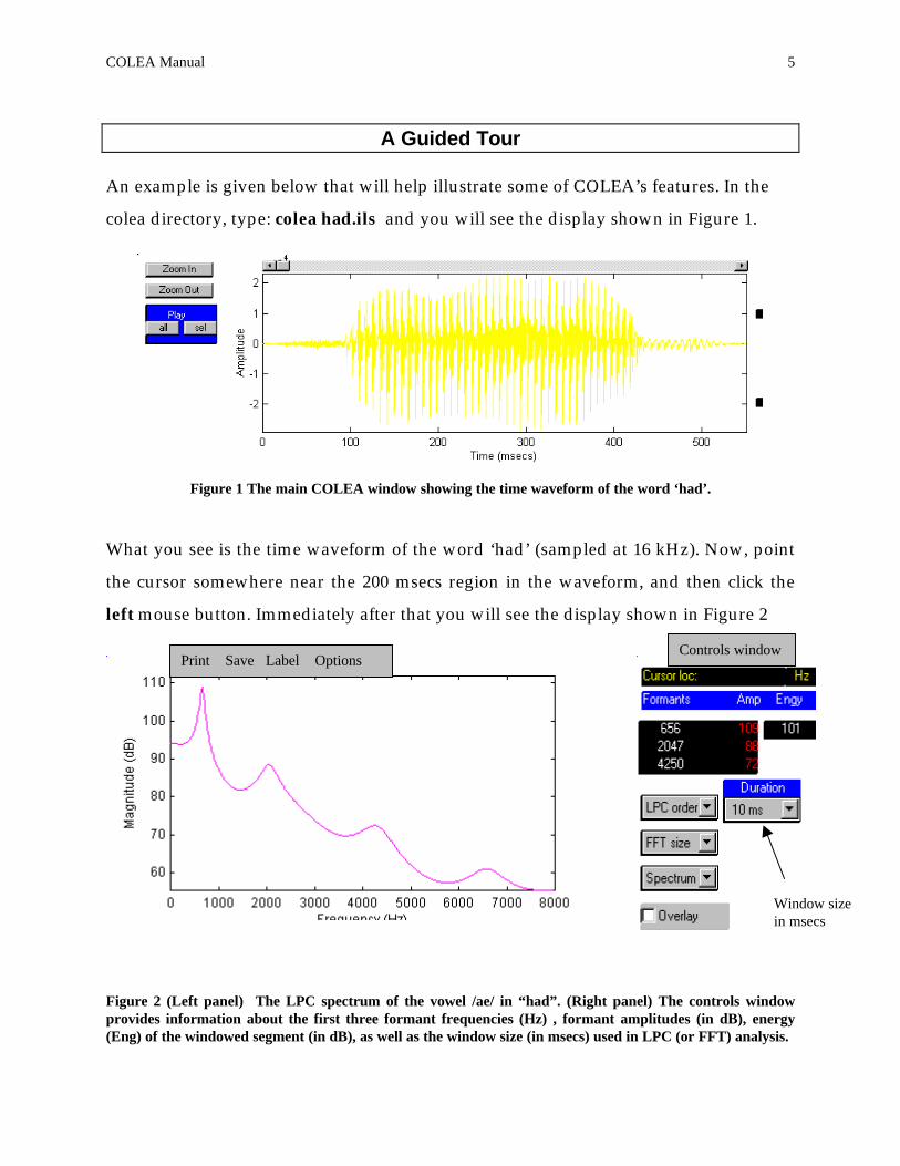
An example is given below that will help illustrate some of COLEA’s features. In the
colea directory, type: colea had.ils and you will see the display shown in Figure 1.
Figure 1 The main COLEA window showing the time waveform of the word ‘had’.
What you see is the time waveform of the word ‘had’ (sampled at 16 kHz). Now, point
the cursor somewhere near the 200 msecs region in the waveform, and then click the
left mouse button. Immediately after that you will see the display shown in Figure 2
Figure 2 (Left panel) The LPC spectrum of the vowel /ae/ in “had”. (Right panel) The controls windowprovides information about the first three formant frequencies (Hz) , formant amplitudes (in dB), energy(Eng) of the windowed segment (in dB), as well as the window size (in msecs) used in LPC (or FFT) analysis.
Window sizein msecs
Print Save Label OptionsControls window

COLEA Manual 6
appearing at the bottom of the screen. This spectrum was obtained by performing a 12-
pole LPC analysis on the 10-msec speech segment taken right of the cursor. So, when you
click anywhere on the waveform using the left mouse button, the program takes a 10-
msec window of the speech segment immediately after the cursor line, and performs
LPC analysis. You may change the size of the window, using the Duration pull-down
option shown in the controls window (Fig. 2, right panel).
Controls window optionsAmong other things, the controls window in Figure 2 displays estimates of the
formant frequencies and formant amplitudes (in dB). The formant frequencies are
computed by peak-picking the LPC spectrum. To get accurate estimates of the formant
frequencies, one needs to choose the LPC order properly depending on the sampling
frequency. Although 12-pole LPC analysis is typically adequate for telephone speech, it
is not adequate for speech recorded at sampling frequencies of 16 kHz or above. In the
example above (Fig. 2) the LPC order was 12, and the third formant (F3) had a value of
F3=4250 Hz, which is suspiciously high for a third formant (for an adult male speaker).
Increasing the LPC order to 18 will yield a better estimate of the second and third
formants for this example. The LPC order can be increased using the ‘LPC order’ pull-
down option in the controls window (Fig. 2).
If you want to see the FFT spectrum instead of the LPC spectrum, you can do
that by selecting ‘FFT’ in the ‘Spectrum’ pull-down option in the controls window.
After selecting the FFT spectrum, you have a choice on the size of the FFT using the
‘FFT size’ option in the controls window.
If you want to see the FFT spectrum overlaid on top of the LPC spectrum, then
click on the ‘Overlay’ box in the controls window. The ‘Overlay’ box in Figure 2 can
also be used for overlaying several spectra for comparative purposes. When checking
the ‘Overlay’ box the current LPC display (Figure 2) freezes, and any subsequent
spectra are overlaid on top of previous displays. To try out this option, check the
‘Overlay’ box and click with the left mouse button somewhere in the waveform. In

COLEA Manual 7
order to get back to the single-display-at-a-time mode, check the ‘Overlay’ box one
more time.
When you click anywhere in the LPC spectrum window using the left mouse
button, you will see the cursor location (Cursor loc) in Hz in the controls window.
LPC Spectrum windowThere are four pull-down menus in the LPC spectrum window (Fig. 2): Print |
Save | Label | Options
The Print and Save options are used for printing or saving the spectra in the LPC
window in several formats including postscript, windows metafile, etc.
The Label menu is used for adding text or legends on the figure or deleting existing
text in the figure. To add text on the figure, select ‘Add text’ and then you will see a
small text window, in which you type the text you want to add in the figure. After
typing the text, hit the <Enter> key, and then point the cross-line cursor at the location
in the LPC window where you want to insert the text, and click the left mouse button.
To delete the last text inserted in the figure, use the ‘Delete text’ option.
The Options menu has the following sub-menus: -Set frequency range
-LPC analysis -..
-FFT analysis -..
The ‘Set Frequency Range’ sub-menu is used for setting the frequency range. In the
example above (Fig. 2) the frequency range was 0-8000 Hz, that is, it was 0-Fs/2, where
Fs is the sampling frequency. If you want to see the spectrum in the range, say, 0- 5kHz,
then you may do so using the ‘Set frequency range’ sub-menu.
The ‘LPC analysis’ sub-menu is for setting a few options in LPC analysis such as using
(or not using) a pre-emphasis FIR filter of the form H z z( ) .= − −1 0 97 1 , and using
COLEA Manual 8
Hamming or rectangular window. The ‘FFT analysis’ menu has the same options, in
addition to displaying the spectrum using lines or in picket-like form.
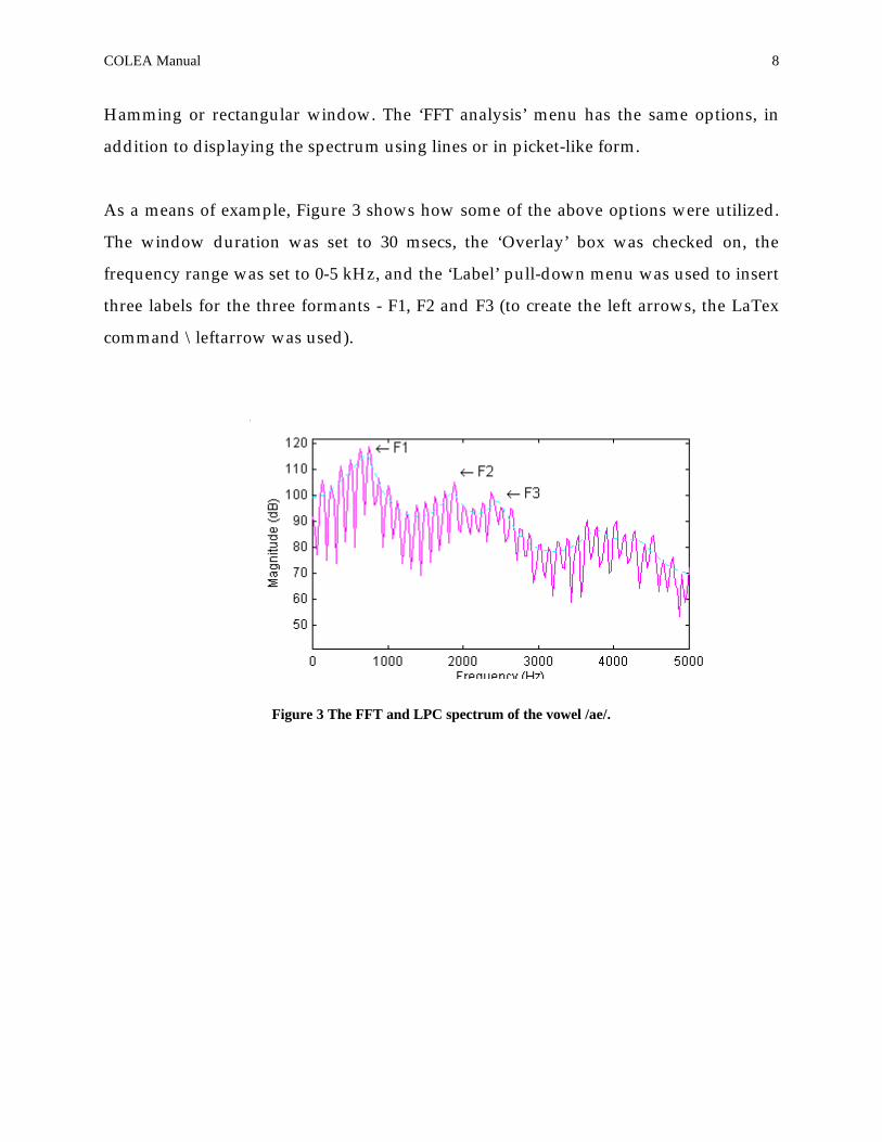
As a means of example, Figure 3 shows how some of the above options were utilized.
The window duration was set to 30 msecs, the ‘Overlay’ box was checked on, the
frequency range was set to 0-5 kHz, and the ‘Label’ pull-down menu was used to insert
three labels for the three formants - F1, F2 and F3 (to create the left arrows, the LaTex
command \leftarrow was used).
Figure 3 The FFT and LPC spectrum of the vowel /ae/.
COLEA Manual 9
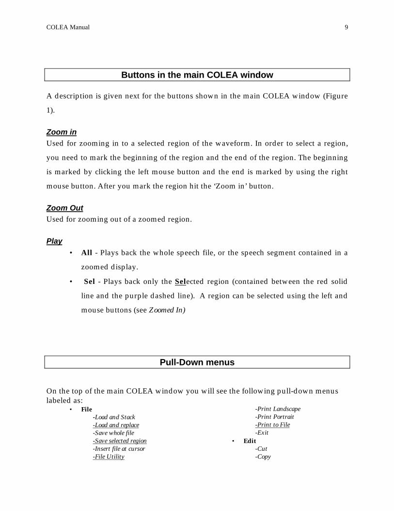
Buttons in the main COLEA window
A description is given next for the buttons shown in the main COLEA window (Figure
1).
Zoom inUsed for zooming in to a selected region of the waveform. In order to select a region,
you need to mark the beginning of the region and the end of the region. The beginning
is marked by clicking the left mouse button and the end is marked by using the right
mouse button. After you mark the region hit the ‘Zoom in’ button.
Zoom OutUsed for zooming out of a zoomed region.
Play• All - Plays back the whole speech file, or the speech segment contained in a
zoomed display.
• Sel - Plays back only the Selected region (contained between the red solid
line and the purple dashed line). A region can be selected using the left and
mouse buttons (see Zoomed In)
Pull-Down menus
On the top of the main COLEA window you will see the following pull-down menuslabeled as:
• File -Load and Stack
-Load and replace-Save whole file-Save selected region-Insert file at cursor-File Utility
-Print Landscape-Print Portrait-Print to File-Exit
• Edit-Cut-Copy

COLEA Manual 10
-Paste-Zero segment-Amplify or attenuate segment-Insert silence at cursor
• Display-Time waveform-Spectrogram-Single window-Energy plot-F0 contour-Formant track-Power Spectral Density-Preferences
• Record
• Tools-Add white noise-Add noise from file-Convert to SCN noise-Filter tool-Sinewave generator-Label tool-Comparison tool-Volume control
A brief explanation of some of these options is given next.
FILE
Load and StackThis option in the FILE menu is used for displaying two files (see Figure 4). The
COLEA window is split in to two smaller windows. The top window displays the new
speech file, while the bottom window displays the old speech file. The top window can
be selected by clicking, using the right mouse button, the top waveform. Likewise, the
bottom window can be selected by clicking, using the right mouse button, the bottom
waveform. A small yellow box appears next to the selected window, and this is how
you know which of the two windows is active. So, if for example you want to listen to
the top waveform, just click anywhere in the top waveform using the right mouse
button, and then click on the ‘Play’ button. In order to switch to a single-window
display, choose from the DISPLAY menu, Single window.
Figure 4 The ‘Load and stack’ option from the FILE menu can be used to display two speech files.

COLEA Manual 11
Load and replace
The ‘Load and replace’ option in the FILE menu loads a new file which replaces
the old file. The new speech file is displayed in single-window mode, as in Fig. 1.
Save selected regionThis option allows you to save a selected speech segment (the selection is made
using the left and right mouse buttons) to a file. It is very important that the given
filename has the same file extension as the original file.
Insert file at cursorThe ‘Insert file at cursor’ option allows you to insert another file at a cursor
location specified with the left mouse button.
File UtilityThe ‘File Utility’ (shown to the
right) is used for upsampling or
downsampling the speech signal,
for swapping bytes or for changing
the sampling frequency and the size
of the header.
EDITThe EDIT menu allows you to cut, copy as well as paste selected segments of the
time waveform. Before using this menu you need to select first, using the left and right
mouse buttons, the speech segment that you would like cut or copied. To paste a

COLEA Manual 12
selected segment, click the left mouse button at the location where you want to insert
the new segment, and then choose the “paste” option from the EDIT menu.
Zero segmentThe ‘Zero segment’ option is used
for zeroing a selected speech
segment, as shown in the figure
on the right.
Amplify/AttenuateThis option is used for amplifying or attenuating selected speech segments by a factor
of 2 or ½ respectively.
Insert silence at cursorThe ‘Insert silence at cursor’ option is used for inserting X msecs of silence at the cursor,
where X is the number of msecs specified by the user.
DISPLAY
SpectrogramThis option displays the spectrogram (in color or in gray scale) of the speech signal. The
default frequency range for spectrogram display is 0-5 kHz. To display full range, i.e.,
from 0-Fs/2, use the ‘Full range’ option from the Spectrogram submenu. To switch back
to the time waveform select the ‘Time waveform’ option from the DISPLAY menu.
Zeroed segment

COLEA Manual 13
Energy plotThis option is used for displaying the energy contour computed every 20-msec
intervals, and expressed in dB.
F0 contour (pitch contour)The pitch contour can be computed using either the autocorrelation method or the
cepstrum method [1][2]. A simplified implementation of the cepstrum approach is used
here. In the original method proposed by Noll [2], a great number of rules was used to
preserve pitch
continuity or avoid
pitch doubling errors.
No such rules are
used in the present
implementation. The
pitch contour for the
example file ‘had.ils’
is shown in the figure on the right. The average F0 is displayed in the title of the
Figure window.
The user has the option of saving the F0 values in a file, by clicking on the ‘Save pitch
values’ option next to the ‘Help’ menu of the pitch contour window.
Formant trackThis option displays the formant track of a selected speech segment or the formant
track of the whole speech file. Formant frequencies (F1, F2 and F3) are computed by
solving for the roots of the LPC polynomial [3]. Heuristic rules are used to ensure

COLEA Manual 14
formant continuity between frames. The user has the option of saving the formant
frequency values in a file, by clicking on the ‘Save formants’ option next to the ‘Help’
menu of the formant track window. The two figures below show the spectrogram of
the vowel /ae/ in “had”, and the corresponding formant track.
Power Spectral Density
This option displays an estimate of the power spectral density (long-time average FFT
spectrum) obtained using Welch’s method.
F1
F2
F3
Save formants
COLEA Manual 15
RECORDThis option calls Windows’ record program from COLEA. It therefore allows
you to record a new speech file without having to exit colea. You can also configure the
‘Record’ option to call a more sophisticated record/playback program (e.g., the
WaveEditor from SoundBlaster). To do that, edit the file ‘sndcard.cfg’ (in the colea
directory) and put the name (including the path) of the record program.
TOOLSThis menu provides some tools for adding noise, filtering, comparing
waveforms, and manually segmenting waveforms.
Add white noiseThis option adds white Gaussian noise to the signal at an SNR specified by the user.
After selecting this option, a small window will appear in which you enter the SNR in
dB. After typing the SNR value, hit the <Enter> key.
Add noise from a fileThis option adds noise to the speech signal at an SNR specified by the user. The noise is
read from a file specified by the user.
Convert to SCN noiseThis option converts the speech signal to Signal Correlated Noise (SCN) using a
method proposed by Schroeder. This method preserves the shape of the time
waveform, but destroys the spectral content of the signal.
Filter toolThis tool can be used to low-pass, high-pass or bandpass the speech signal. The Filter
Tool window is shown in Figure 5. You may enter the cutoff frequency as well as the

COLEA Manual 16
order of the Butterworth filter. Typically, the higher the filter order the steeper the filter
roll-off. After entering the cutoff frequency, hit the ‘Apply filter’ button to filter the
signal. The COLEA window will then be split in two smaller windows, the top being
the filtered signal and the bottom being the original (unfiltered) signal.
Figure 5 The Filter Tool window. This tool can be used to low-pass, high-pass or band-pass the signal atcutoff frequencies specified by the user.
Sinewave generatorThis tool generates sinewaves of various frequencies,
amplitudes and durations all specified by the user (see figure on
the right). After entering the desired frequency, hit the “Apply”
button. The generated sinewaves are tapered at the beginning
and end to avoid any clicks.
Label ToolThis tool can be used for manual segmentation of speech
waveforms as well as for displaying time-aligned label files

COLEA Manual 17
(e.g., TIMIT’s .phn files). For instance, this tool can be used to create label files needed
for training speech recognition systems.
To load a label file, click on the ‘Load labels’ button, and specify the label file. The label
files need to be in TIMIT format, that is, they should have the following format:
FromSample ToSample LabelText
…
Example:
0 12000 will
12001 15000 go
The first two numbers in each line are the sample boundaries of the phoneme or word
indicated. Figure 6 below shows as an example the time waveform of the TIMIT file
‘sentence.wav’ (included with the colea program) aligned with the corresponding
phonetic transcription file ‘sentence.phn’ (also included).
Figure 6 Portion of the waveform of the TIMIT sentence “Will you please confirm government policyregarding waste removal? “ time-aligned with its phonetic transcription using the ‘Load labels’ option of theLabel Tool.

COLEA Manual 18
To create a label file, first click on the ‘Add label’ button, then point the cursor to the
beginning of the word (or phoneme, etc.) and press the left mouse button. Next, point
the cursor to the end of the word (or phoneme, etc.) and press the right mouse button.
A text window should be created which will have the length of the word or phoneme.
Enter in the text window the word or phoneme label and hit the <Enter> key. After
creating all the labels, then press the ‘Save Labels’ button to save the labels in a file in
TIMIT format. The figure below shows as an example the labels created for the word
“had” - /h ae d/.
Figure 7 Example of manual segmentation of the word ‘had’ (/h ae d/) using the Label tool.
Comparison ToolThis tool is used for comparing two
waveforms or two frames using either time-
domain measures (i.e., SNR) or spectral
domain measures (i.e., Itakura-Saito measure)
[4][5].
To use this tool, you need first to load two

COLEA Manual 19
waveforms (using the Load and Stack option in the FILE menu), where the top is the
approximated (e.g., coded or enhanced) waveform and the bottom waveform is the
original waveform.
The user has the option of making an overall (or global) comparison between
the two waveforms or a segmental (local) comparison between the two waveforms. The
first option is in effect when clicking the button ‘Overall’ (see figure above). In this
option, the two speech files are segmented in 10 msec frames (default frame size), and
the comparison is performed for each frame. After selecting the distance measure to
use, a window is opened at the bottom of the screen showing the values of the
distortion measure evaluated every 10-msec frame. To change the default frame size,
enter the new value (in msecs) in the ‘Analysis frame’ box shown in the Figure above.
In order to compare two particular speech segments of the two files, point to the
beginning of the segment and press the left mouse button. Use the bottom window to
indicate the beginning of the segment. Then, click on the ‘Cursor’ button (see Figure
above), and select the distance measure. A new window will immediately open
showing the LPC spectra of the two files. The top spectrum is the LPC spectrum of the
original file. The value of the distance measure will be shown as a title.
Most of the spectral distortion measures are based on LPC analysis of order 14.
To change the LPC order, edit the ‘Order, N’ box (see Figure above) and enter the new
value. The following distance measures are used [4][5]:
SNR – Signal-to-noise ratio
CEP - Cepstrum
WCEP - Weighted cepstrum (by a ramp)
IS - Itakura-Saito
LR - Likelihood ratio
LLR - Log-likelihood ratio
WLR - Weighted likelihood ratio
WSM - Weighted slope distance metric (Klatt's) [6].

COLEA Manual 20
Volume control
This tool is used for adjusting the volume.
There are three different modes:
♦ Autoscale (default)
The signal is automatically scaled
to the maximum value allowed by the hardware. In this mode, you can not use
the slider bar.
♦ No scale
In this mode the signal can be made louder or softer by moving the slider bar.
♦ Absolute
In this mode, the signal is played as is. No scaling is done. Moving the slider bar
has no effect.

COLEA Manual 21
REFERENCES[1] L. Rabiner and R. Shafer, Digital Processing of Speech Signals, Englewood Cliffs:
Prentice Hall, 1978.
[2] A. Noll, “Cepstrum pitch determination,” J. Acoust. Soc. Am., vol. 41, pp. 293-309,
February 1967.
[3] J.D. Markel and A.H. Gray, Jr., Linear Prediction of Speech, Springer-Verlag, Berlin,
1976.
[4] A.H. Gray and J.D. Markel, “Distance measures for speech processing, IEEE Trans.
Acoustics, Speech, Signal Proc., ASSP-24(5), pp. 380-391, October 1976.
[5] L. Rabiner and B-H. Juang, Fundamentals of Speech Recognition, Englewood Cliffs:
Prentice Hall, 1993.
[6] D. Klatt, “Prediction of perceived phonetic distance from critical band spectra: A
first step,” Proc. ICASSP, pp. 1278-1281, 1982.


