
Classification of Hyperspectral Breast Images for Cancer Detection
Sander Parawira
December 4, 2009
1 Introduction
In 2009 approximately one out of eight women has breast cancer. More than 180,000
women are expected to be diagnosed with breast cancer and more than 40,000 women are
expected to die from it. Most breast cancer deaths can be prevented if it is detected and treated
early. The most common imaging techniques for breast cancer detection are x-ray
mammography and computed tomography (CT). These two methods aim to detect any lumps or
masses in breast tissues that may be cancerous. However, there is an inherent problem associated
with these two methods. They are expensive and involve radiating the breast tissues which may
be dangerous since even small doses of radiation can induce mutation that leads to cancer.
Fourier transform infrared (FTIR) spectroscopy is a measurement technique in which the
absorbance of a tissue sample for many wavelengths is captured using infrared beams. The
purpose of capturing many distinct wavelengths (in our case we capture 1641 wavelengths
corresponding to 720 nm to 4000 nm in 2 nm increments) is so that much more information is
captured. There are three steps involved in performing FTIR: (1) identifying sample regions by
manual inspection using optical microscope (2) applying an opaque mask with an aperture of
controlled size to restrict infrared beam absorption to the area of interest (3) measuring the
attenuation of the incident infrared beam with a detector
In this paper we present a machine learning approach in hyperspectral image analysis for
breast cancer detection. We consider the scenario where a band sequential image of a breast
tissue specimen is collected using FTIR spectroscopy. Our goal is to determine which parts of
the image correspond to cancer cells and which parts of the image correspond to non-cancer
cells. We first discuss spectrum selection and principal component analysis (PCA) to reduce the
dimensionality of the image. We then discuss the implementation of K-means++ clustering
algorithm for data set represented as points in a high dimensional space. We finally add noise to
the image and discuss the robustness of our approach.
2 Dimensionality Reduction
2.1 Subset Selection
The curse of dimensionality tells us that a linear increase in the number of spectrums
used by an algorithm translates into an exponential increase in the number of samples that need
to be processed by the algorithm. From here, we see that utilizing only a subset of the image will
improve the running time significantly. To be exact, we used only 201 bands of the image that
contain the most information, corresponding to the range of wavelengths from 1320 nm to 1720
nm in 2 nm increments.
2.2 Principal Component Analysis (PCA)

PCA is a vector space transform employed to reduce the dimensionality of high
dimensional data set in order to facilitate analysis. PCA is an orthogonal linear transform that
transforms data set into new components such that the greatest variance by any projection of the
data set is in the first component, the second greatest variance by any projection of the data set is
in the second component, and so on.
Suppose that we have a data set � = (��, ��, … , ��). Let the mean and the covariance
matrix of the data set be �� = {�} and �� = {(� − ��)(� − ��)} respectively. We can
determine the eigenvalue �� and corresponding eigenvector �� of �� by solving the equation
���� = ���� for � = 1, 2, … , �. If we want � principal components, then we create a matrix A of
size � × � where the first row of the matrix is the eigenvector corresponding to the greatest
eigenvalue, the second row of the matrix is the eigenvector corresponding to the second greatest
eigenvalue, and so on. The principal components are then given by the equation � = �(� − ��) where the first row is the first principal component, the second row is the second principal
component, and so on.
In our case, we employed PCA to reduce the dimensionality of the data set from 201
dimensions to only 20 dimensions. Consequently, out of 1641 usable spectrums we only utilized
20 bands which are 1.22% of the data set. Figure 2.1 and 2.2 show the first two principal
components.
Figure 2.1: First Principal Component Figure 2.2: Second Principal Component
3 Classification: K-Means++ Clustering Algorithm
The K-Means++ clustering algorithm is an improved variant of K-Means clustering
algorithm with faster convergence. The difference between K-Means++ clustering algorithm and
K-Means clustering algorithm is in the choice of the initial centroids. For K-Means, we choose
the initial centroids randomly. In contrast, for K-Means++, we do the following:
1) Define the radius of a point �, �(�) as the shortest distance from � to an already picked centroid 2) Randomly pick one point in the set as the initial centroid � for cluster 1
3) For each point � in the set, compute �(�) 4) Pick point �′ in the set as the initial centroid � for cluster i with probability
�(�′)" �(�)# ∈ %&'
5) Repeat step 3) and 4) for � = 2, … , ( After we specify the initial centroids, the rest of the algorithm is exactly the same:
1) Compute the distance from each point in the set to each centroid
2) Classify each point in the set to the cluster with shortest distance
3) Update the centroid for each cluster
4) Repeat step 3, 4, 5 until the centroid for each cluster does not change
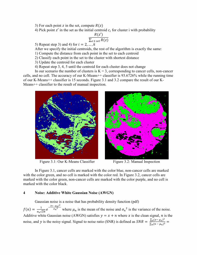
In our scenario the number of clusters is K = 3, corresponding to cancer cells, non-cancer
cells, and no cell. The accuracy of our K-Means++ classifier is 93.6726% while the running time
of our K-Means++ classifier is 15 seconds. Figure 3.1 and 3.2 compare the result of our K-
Means++ classifier to the result of manual inspection.
Figure 3.1: Our K-Means Classifier Figure 3.2: Manual Inspection
In Figure 3.1, cancer cells are marked with the color blue, non-cancer cells are marked
with the color green, and no cell is marked with the color red. In Figure 3.2, cancer cells are
marked with the color green, non-cancer cells are marked with the color purple, and no cell is
marked with the color black.
4 *oise: Additive White Gaussian *oise (AWG*)
Gaussian noise is a noise that has probability density function (pdf)
)(�) = �
*+,�-�
.(+ – 0+)1
2+1 where �� is the mean of the noise and 3�� is the variance of the noise.
Additive white Gaussian noise (AWGN) satisfies � = � + � where � is the clean signal, � is the
noise, and � is the noisy signal. Signal to noise ratio (SNR) is defined as 56� = " (�. 78)1
8
" (� . 7+)1+
=
*8
1
*+1 where �� is the mean of the clean signal and 3�
� is the variance of the clean signal. In our
case, we added an AWGN with mean 0 and variance *8
1
9:; to the image. We ran our K-means
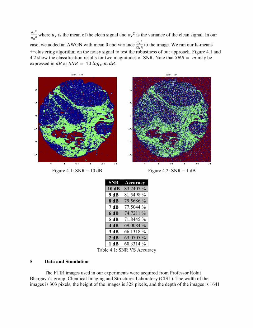
++clustering algorithm on the noisy signal to test the robustness of our approach. Figure 4.1 and
4.2 show the classification results for two magnitudes of SNR. Note that 56� = � may be
expressed in <= as 56� = 10 ?@A�B� <=.
Figure 4.1: SNR = 10 dB Figure 4.2: SNR = 1 dB
S*R Accuracy
10 dB 83.2407 %
9 dB 81.5498 %
8 dB 79.5686 %
7 dB 77.5044 %
6 dB 74.7211 %
5 dB 71.8445 %
4 dB 69.0084 %
3 dB 66.1318 %
2 dB 63.0705 %
1 dB 60.3314 %
Table 4.1: SNR VS Accuracy
5 Data and Simulation
The FTIR images used in our experiments were acquired from Professor Rohit
Bhargava’s group, Chemical Imaging and Structures Laboratory (CISL). The width of the
images is 303 pixels, the height of the images is 328 pixels, and the depth of the images is 1641

bands (spectrums). All of our experiments were done in MATLAB R2008a running on Intel
Centrino 2 T9400 (Dual 2.53 GHz Core).
6 Conclusion and Comparison with Bhargava’s Method
The accuracy of our machine learning approach is 93% when there is no noise and the
accuracy decreases linearly as SNR decreases. On the other hand, Bhargava’s method have
slightly better accuracy at 99% when there is no noise but the accuracy decreases exponentially
as SNR decreases. In terms of running time, our machine learning approach is much faster at 15
seconds compared to Bhargava’s method at 20 hours.
95% of our classification errors come from false positives and the remaining 5% come
from false negatives. This means that in the event of classification error, 95% of the time our
machine learning approach labels non-cancer cells or no cell as cancer cells while 5% of the time
our machine learning approach labels cancer cells as non-cancer cells or no cell. If our machine
learning approach does not detect the presence of any cancer cells, then it is safe to say that no
cancer cell exists in the FTIR images since in our experiments only 0.35% of all cancer cells are
not identified. This is good news because this implies that our machine learning approach can be
used as a first screening criterion before the FTIR images are fed into more expensive techniques
with higher accuracy such as Bhargava’s method.
Furthermore, when it is not possible to obtain FTIR images with no noise, Bhargava’s
method cannot be used since it is very sensitive to noise. Conversely, our machine learning
approach is still a viable option since it is not very susceptible to noise. In summary, the
advantages of our machine learning approach compared to Bhargava’s method lie in its faster
running time and more robustness to noise.
7 References
[1] D. Landgrebe, “Hyperspectral image data analysis as a high dimensional signal processing
problem,” IEEE Signal Processing Magazine, vol. 19, no. 1, pp.17-28, January 2002.
[2] D.C. Fernandez, R. Bhargava, S.M. Hewitt, and I.W. Levin, “Infrared spectroscopic imaging
for observer –invariant hispathology,” �at. Biotechnol., vol. 23, no. 4, pp. 469-473, April 2005.
[3] D. Arthur and S. Vassilvitskii, “K-means++: The advantages of careful seeding,” ACM-SIAM
Symposium on Discrete Algorithms, January 2007.
[4] G. Srinivasan and R. Bhargava , “Fourier transform-infrared spectroscopic imaging: The
emerging evolution from a microscopy tool to a cancer imaging modality,” Spectroscopy, vol.
22, no. 7, pp. 30, July 2007.
[5] I.W. Levin and R. Bhargava, “Fourier transform infrared vibrational spectroscopic imaging:
Integrating miscroscopy and molecular recognition,” Annu. Rev. Phys. Chem, vol. 56, pp. 429-
474, January 2005.
[6] R. Bhargava, “Towards a practical Fourier transform infrared chemical imaging protocol for
cancer hispathology,” Anal. Bioanal. Chem., vol. 389, no. 4, pp. 1155-1169, Septermber 2007.


