
Classical and Quantum Nonlinear Optical Information Processing
Thesis by
Mankei Tsang
In Partial Fulfillment of the Requirements
for the Degree of
Doctor of Philosophy
California Institute of Technology
Pasadena, California
2006
(Defended May 2, 2006)

ii
c© 2006
Mankei Tsang
All Rights Reserved

iii
Acknowledgements
First and foremost I would like to thank my mentor, ProfessorDemetri Psaltis, for giving me the opportunity
to come to Caltech and for his insightful advice about optics, research, and all aspects of life in academia. It
has truly been a pleasure working with him in my four years at Caltech.
I would also like to acknowledge my past and present group mates, who are all intelligent and capable,
and from whom I have learned a great deal. I am especially grateful to Dr. Ye Pu and Dr. Martin Centurion,
for their guidance when I worked briefly in the lab and for sharing with me their exciting experiment results;
Jim Adleman and Dr. David Erickson, for all the driving in a long but enjoyable road trip to the DARPA
workship in Sonoma; Lucinda Acosta, for her help in administrative tasks; and Yayun Liu, for her words of
encouragement when I first started at Caltech. Furthermore,I would like to acknowledge Dr. Zhiwen Liu, Dr.
Hung-Te Hsieh, Zhenyu Li, Hua Long, Troy Rockwood, Eric Ostby, Xin Heng, Baiyang Li, Dr. Allen Pu,
Jae-Woo Choi, and Ted Dikaliotis, with whom I have enjoyed countless inspiring discussions.
I am indebted to Dr. Fiorenzo Omenetto, who provided his experimental results for my first paper, and
generously lent us his experimental equipment several times; Professor Michael Cross, for his advice on the
metaphoric optical computing project; and my candidacy andthesis examining committee members, includ-
ing Professor Amnon Yariv, Professor Changhuei Yang, Professor Oskar Painter, Professor Kerry Vahala, and
Dr. John Hong, for their valuable time, as well as their insightful feedback on my research.
I will forever be indebted to my mother, whose love, care, andsupport make me the person I am now,
despite all the adversities she has had to face. I am also grateful to my elder sister, and all my relatives and
friends in Hong Kong and the United States, who are extremelysupportive of my family and myself.
Last but not the least, I thank my girlfriend, Helen. Withouther I would not have survived a single day at
Caltech.

iv
List of Publications
[1] M. Tsang and D. Psaltis, “Dispersion and nonlinearity compensation by spectral phase conjugation,”
Opt. Lett.28, 1558 (2003).
[2] M. Tsang, D. Psaltis, and F. G. Omenetto, “Reverse propagation of femtosecond pulses in optical
fibers,” Opt. Lett.28, 1873 (2003).
[3] M. Tsang and D. Psaltis, “Spectral phase conjugation with cross-phase modulation compensation,”
Opt. Express12, 2207 (2004).
[4] M. Tsang and D. Psaltis, “Spectral phase conjugation by quasi-phase-matched three-wave mixing,”
Opt. Commun.242, 659 (2004).
[5] M. Tsang and D. Psaltis, “Spontaneous spectral phase conjugation for coincident frequency entangle-
ment,” Phys. Rev. A71, 043806 (2005).
[6] M. Centurion, Y. Pu, M. Tsang, and D. Psaltis, “Dynamics of filament formation in a Kerr medium,”
Phys. Rev. A71, 063811 (2005).
[7] M. Tsang, “Spectral phase conjugation via extended phase matching,” J. Opt. Soc. Am. B23, 861
(2006).
[8] M. Tsang and D. Psaltis, “Propagation of temporal entanglement,” Phys. Rev. A73, 013822 (2006).
[9] M. Tsang, “Quantum temporal correlations and entanglement via adiabatic control of vector solitons,”
e-print quant-ph/0603088 [submitted to Phys. Rev. Lett. ].
[10] M. Tsang and D. Psaltis, “Reflectionless evanescent wave amplification via two dielectric planar wave-
guides,” e-print physics/0603079 [submitted to Opt. Lett.].
[11] M. Tsang, “Beating the spatial standard quantum limitsvia adiabatic soliton expansion and negative
refraction,” under preparation.
[12] M. Tsang and D. Psaltis, “Metaphoric optical computingof fluid dynamics,” under preparation.
v
Abstract
This thesis is a theoretical investigation of the classicaland quantum information processing enabled by the
advent of modern ultrafast nonlinear optics.
Chapter 2 and 3 study the propagation of ultrashort optical pulses in optical fibers, and propose two meth-
ods of compensating the linear and nonlinear distortions experienced by the pulses, namely, reverse propaga-
tion and spectral phase conjugation. Chapter 4 and 5 suggestdifferent schemes that implement spectral phase
conjugation.
Chapter 6 and 7 establish the connection between classical spectral phase conjugation and quantum co-
incident frequency entanglement. Chapter 6 shows how a spectral phase conjugator can create coincident
frequency entangled photon pairs, and Chapter 7 in turn demonstrates how a coincident frequency entangle-
ment generator can perform spectral phase conjugation.
The next three chapters, 8, 9, and 10, focus on quantum spatiotemporal information processing. Chapter
8 studies the temporal properties of entangled photon pair propagation and proposes the concept of quantum
temporal imaging. Chapter 9 investigates how optical solitons can be used to perform quantum timing jitter
reduction and temporal entanglement, while Chapter 10 applies the same idea to the spatial domain for
quantum spatial information processing tasks, such as spatial beam displacement uncertainty reduction and
quantum lithography.
The final two chapters return to a couple of miscellaneous problems in classical optics. Chapter 11
shows how a pair of dielectric slabs can amplify the near fieldof an optical image. Chapter 12 explores the
similarities between nonlinear optics and fluid dynamics, and speculates on the possibility of using nonlinear
optics experiments to simulate fluid dynamics problems.
vi
Contents
Acknowledgements iii
List of Publications iv
Abstract v
1 Summary 1
Bibliography 3
2 Reverse propagation of femtosecond pulses in optical fibers 4
2.1 Introduction . . . . . . . . . . . . . . . . . . . . . . . . . . . . . . . . . . . .. . . . . . . 4
2.2 Theory . . . . . . . . . . . . . . . . . . . . . . . . . . . . . . . . . . . . . . . . . .. . . . 5
2.3 Comparison with experiments . . . . . . . . . . . . . . . . . . . . . . .. . . . . . . . . . 6
2.4 Numerical analysis . . . . . . . . . . . . . . . . . . . . . . . . . . . . . . .. . . . . . . . 7
2.5 Conclusion . . . . . . . . . . . . . . . . . . . . . . . . . . . . . . . . . . . . . .. . . . . 8
Bibliography 11
3 Dispersion and nonlinearity compensation via spectral phase conjugation 12
3.1 Introduction . . . . . . . . . . . . . . . . . . . . . . . . . . . . . . . . . . . .. . . . . . . 12
3.2 Theory . . . . . . . . . . . . . . . . . . . . . . . . . . . . . . . . . . . . . . . . . .. . . . 13
3.3 Numerical analysis . . . . . . . . . . . . . . . . . . . . . . . . . . . . . . .. . . . . . . . 15
3.4 Conclusion . . . . . . . . . . . . . . . . . . . . . . . . . . . . . . . . . . . . . .. . . . . 17
Bibliography 18
4 Spectral phase conjugation with cross-phase modulation compensation 19
4.1 Introduction . . . . . . . . . . . . . . . . . . . . . . . . . . . . . . . . . . . .. . . . . . . 19
4.2 Spectral phase conjugation by four-wave mixing . . . . . . .. . . . . . . . . . . . . . . . . 20
4.3 High conversion efficiency with signal amplification . . .. . . . . . . . . . . . . . . . . . . 21
4.4 Cross-phase modulation compensation . . . . . . . . . . . . . . .. . . . . . . . . . . . . . 24

vii
4.5 Numerical analysis . . . . . . . . . . . . . . . . . . . . . . . . . . . . . . .. . . . . . . . 26
4.5.1 Conversion efficiency . . . . . . . . . . . . . . . . . . . . . . . . . . .. . . . . . . 28
4.5.2 Demonstration of cross-phase modulation compensation . . . . . . . . . . . . . . . 28
4.6 Beyond the basic assumptions . . . . . . . . . . . . . . . . . . . . . . .. . . . . . . . . . 30
4.6.1 Pump depletion . . . . . . . . . . . . . . . . . . . . . . . . . . . . . . . . .. . . . 30
4.6.2 Other nonideal conditions . . . . . . . . . . . . . . . . . . . . . . .. . . . . . . . 30
4.7 Conclusion . . . . . . . . . . . . . . . . . . . . . . . . . . . . . . . . . . . . . .. . . . . 31
Bibliography 32
5 Spectral phase conjugation by quasi-phase-matched three-wave mixing 33
5.1 Introduction . . . . . . . . . . . . . . . . . . . . . . . . . . . . . . . . . . . .. . . . . . . 33
5.2 Configuration . . . . . . . . . . . . . . . . . . . . . . . . . . . . . . . . . . . .. . . . . . 34
5.3 Theory . . . . . . . . . . . . . . . . . . . . . . . . . . . . . . . . . . . . . . . . . .. . . . 34
5.4 Comparison with the FWM scheme . . . . . . . . . . . . . . . . . . . . . . .. . . . . . . 36
5.5 Numerical analysis . . . . . . . . . . . . . . . . . . . . . . . . . . . . . . .. . . . . . . . 37
5.6 Competing third-order nonlinearity . . . . . . . . . . . . . . . .. . . . . . . . . . . . . . . 38
5.7 Conclusion . . . . . . . . . . . . . . . . . . . . . . . . . . . . . . . . . . . . . .. . . . . 39
Bibliography 40
6 Spontaneous spectral phase conjugation for coincident frequency entanglement 42
6.1 Introduction . . . . . . . . . . . . . . . . . . . . . . . . . . . . . . . . . . . .. . . . . . . 42
6.2 Configurations . . . . . . . . . . . . . . . . . . . . . . . . . . . . . . . . . . .. . . . . . . 43
6.3 Conversion efficiency . . . . . . . . . . . . . . . . . . . . . . . . . . . . .. . . . . . . . . 45
6.4 Hong-Ou-Mandel interferometry . . . . . . . . . . . . . . . . . . . .. . . . . . . . . . . . 47
6.5 Conclusion . . . . . . . . . . . . . . . . . . . . . . . . . . . . . . . . . . . . . .. . . . . 50
Bibliography 51
7 Spectral phase conjugation via extended phase matching 53
7.1 Introduction . . . . . . . . . . . . . . . . . . . . . . . . . . . . . . . . . . . .. . . . . . . 53
7.2 Setup . . . . . . . . . . . . . . . . . . . . . . . . . . . . . . . . . . . . . . . . . . .. . . 54
7.3 Fourier analysis . . . . . . . . . . . . . . . . . . . . . . . . . . . . . . . . .. . . . . . . . 55
7.4 Laplace analysis . . . . . . . . . . . . . . . . . . . . . . . . . . . . . . . . .. . . . . . . . 58
7.5 Spontaneous parametric down conversion . . . . . . . . . . . . .. . . . . . . . . . . . . . 60
7.6 Numerical analysis . . . . . . . . . . . . . . . . . . . . . . . . . . . . . . .. . . . . . . . 61
7.7 Conclusion . . . . . . . . . . . . . . . . . . . . . . . . . . . . . . . . . . . . . .. . . . . 64
viii
Bibliography 65
8 Propagation of temporal entanglement 67
8.1 Introduction . . . . . . . . . . . . . . . . . . . . . . . . . . . . . . . . . . . .. . . . . . . 67
8.2 Two photons in two separate modes . . . . . . . . . . . . . . . . . . . .. . . . . . . . . . 68
8.3 Quantum temporal imaging . . . . . . . . . . . . . . . . . . . . . . . . . .. . . . . . . . . 71
8.4 Two photons in two linearly coupled modes . . . . . . . . . . . . .. . . . . . . . . . . . . 75
8.5 Two photons in many modes . . . . . . . . . . . . . . . . . . . . . . . . . . .. . . . . . . 77
8.6 Four-wave mixing . . . . . . . . . . . . . . . . . . . . . . . . . . . . . . . . .. . . . . . . 78
8.7 Two-photon vector solitons . . . . . . . . . . . . . . . . . . . . . . . .. . . . . . . . . . 79
8.8 Conclusion . . . . . . . . . . . . . . . . . . . . . . . . . . . . . . . . . . . . . .. . . . . 81
Bibliography 82
9 Quantum temporal correlations and entanglement via adiabatic control of vector solitons 84
9.1 Introduction . . . . . . . . . . . . . . . . . . . . . . . . . . . . . . . . . . . .. . . . . . . 84
9.2 Theory . . . . . . . . . . . . . . . . . . . . . . . . . . . . . . . . . . . . . . . . . .. . . . 85
9.2.1 Formalism . . . . . . . . . . . . . . . . . . . . . . . . . . . . . . . . . . . . .. . 85
9.2.2 Adiabatic soliton expansion . . . . . . . . . . . . . . . . . . . . .. . . . . . . . . 87
9.2.3 Quantum dispersion compensation . . . . . . . . . . . . . . . . .. . . . . . . . . . 88
9.3 Temporal correlations among photons . . . . . . . . . . . . . . . .. . . . . . . . . . . . . 89
9.4 Temporal entanglement between optical pulses . . . . . . . .. . . . . . . . . . . . . . . . 90
Bibliography 92
10 Beating the spatial standard quantum limits via adiabatic soliton expansion and negative re-
fraction 94
10.1 Introduction . . . . . . . . . . . . . . . . . . . . . . . . . . . . . . . . . . .. . . . . . . . 94
10.2 Formalism . . . . . . . . . . . . . . . . . . . . . . . . . . . . . . . . . . . . . .. . . . . . 95
10.3 Multiphoton absorption rate of nonclassical states . .. . . . . . . . . . . . . . . . . . . . . 98
10.4 Generating nonclassical states via the soliton effect. . . . . . . . . . . . . . . . . . . . . . 99
10.5 Conclusion . . . . . . . . . . . . . . . . . . . . . . . . . . . . . . . . . . . . .. . . . . . 101
Bibliography 102
11 Reflectionless evanescent wave amplification via two dielectric planar waveguides 103
11.1 Introduction . . . . . . . . . . . . . . . . . . . . . . . . . . . . . . . . . . .. . . . . . . . 103
11.2 Evanescent wave amplification . . . . . . . . . . . . . . . . . . . . .. . . . . . . . . . . . 104
11.2.1 Evanescent wave amplification by one dielectric slab. . . . . . . . . . . . . . . . . 104
ix
11.2.2 Reflectionless evanescent wave amplification by two waveguides . . . . . . . . . . . 106
11.3 Discussion . . . . . . . . . . . . . . . . . . . . . . . . . . . . . . . . . . . . .. . . . . . . 107
11.4 Conclusion . . . . . . . . . . . . . . . . . . . . . . . . . . . . . . . . . . . . .. . . . . . 108
Bibliography 109
12 Metaphoric optical computing of fluid dynamics 110
12.1 Introduction . . . . . . . . . . . . . . . . . . . . . . . . . . . . . . . . . . .. . . . . . . . 110
12.1.1 Philosophy of metaphoric computing . . . . . . . . . . . . . .. . . . . . . . . . . 110
12.1.2 Correspondence between nonlinear optics and fluid dynamics . . . . . . . . . . . . 111
12.2 Correspondence between nonlinear optics and Euler fluid dynamics . . . . . . . . . . . . . 113
12.2.1 Madelung transformation . . . . . . . . . . . . . . . . . . . . . . .. . . . . . . . . 113
12.2.2 Vorticity . . . . . . . . . . . . . . . . . . . . . . . . . . . . . . . . . . . .. . . . . 115
12.2.3 Optical vortex solitons and point vortices . . . . . . . .. . . . . . . . . . . . . . . 116
12.2.4 The fluid flux representation . . . . . . . . . . . . . . . . . . . . .. . . . . . . . . 118
12.2.5 Optical vortex solitons and vortex blobs . . . . . . . . . .. . . . . . . . . . . . . . 119
12.2.6 Numerical evidence of correspondence between nonlinear optics and Euler fluid dy-
namics . . . . . . . . . . . . . . . . . . . . . . . . . . . . . . . . . . . . . . . . . 121
12.3 Similarities between nonlinear Schrodinger dynamics and Navier-Stokes fluid dynamics . . 121
12.3.1 Zero-flux boundary conditions, boundary layers, andboundary layer separation . . . 122
12.3.2 Dissipation of eddies . . . . . . . . . . . . . . . . . . . . . . . . . .. . . . . . . . 123
12.3.3 Karman vortex street . . . . . . . . . . . . . . . . . . . . . . . . . . . . . . . . . . 123
12.3.4 Kolmogorov turbulence . . . . . . . . . . . . . . . . . . . . . . . . .. . . . . . . 129
12.4 The split-step method . . . . . . . . . . . . . . . . . . . . . . . . . . . .. . . . . . . . . . 130
12.5 Conclusion . . . . . . . . . . . . . . . . . . . . . . . . . . . . . . . . . . . . .. . . . . . 131
Bibliography 133
x
List of Figures
2.1 Comparison of OPC and reverse propagation. . . . . . . . . . . .. . . . . . . . . . . . . . . 5
2.2 Reverse propagation of an experimental output pulse. The experimental output pulse shape is
plotted atz= 0 m and numerically propagates in reverse fromz= 0 m toz= −10 m. . . . . . 6
2.3 Comparison of the input obtained from reverse propagation and the actual experimental input. 7
2.4 Reverse propagation of a chirped sech pulse atλ0 = 1550 nm. . . . . . . . . . . . . . . . . . 8
2.5 Amplitude and phase of the optimal input that produces the desired sech output pulse shape at
λ0 = 800 nm. . . . . . . . . . . . . . . . . . . . . . . . . . . . . . . . . . . . . . . . . . . . 9
2.6 Compared with the ideal output pulse shape produced by reverse propagation and pulse shap-
ing, the OPC output is significantly distorted by high-ordereffects. . . . . . . . . . . . . . . . 9
3.1 Schematics of TPC and SPC. . . . . . . . . . . . . . . . . . . . . . . . . . .. . . . . . . . 12
3.2 Input and output pulses with and without compensation schemes, when a 1.7 W 200 fs super-
Gaussian pulse propagates for a total distance of 2 km. . . . . .. . . . . . . . . . . . . . . . 16
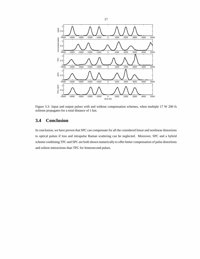
3.3 Input and output pulses with and without compensation schemes, when multiple 17 W 200 fs
solitons propagates for a total distance of 1 km. . . . . . . . . . .. . . . . . . . . . . . . . . 17
4.1 Setup of SPC by four-wave mixing.As(t) is the signal pulse,Ap(t) andAq(t) are the pump
pulses, andAi(t) is the backward-propagating idler pulse. (After Ref. [1]) .. . . . . . . . . . 20
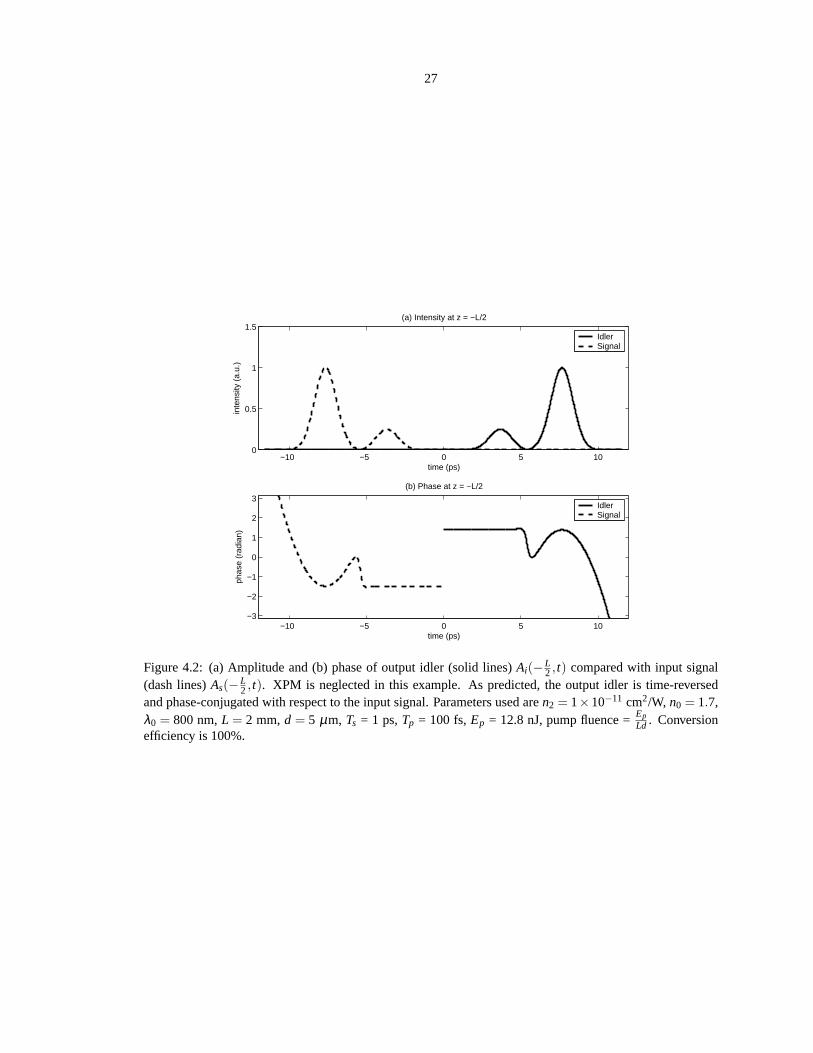
4.2 (a) Amplitude and (b) phase of output idler (solid lines)Ai(−L2 , t) compared with input signal
(dash lines)As(−L2 , t). XPM is neglected in this example. As predicted, the output idler
is time-reversed and phase-conjugated with respect to the input signal. Parameters used are
n2 = 1×10⁻¹¹ cm2/W, n0 = 1.7, λ0 = 800 nm,L = 2 mm,d = 5 µm, Ts = 1 ps,Tp = 100 fs,
Ep = 12.8 nJ, pump fluence =EpLd . Conversion efficiency is 100%. . . . . . . . . . . . . . . . 27
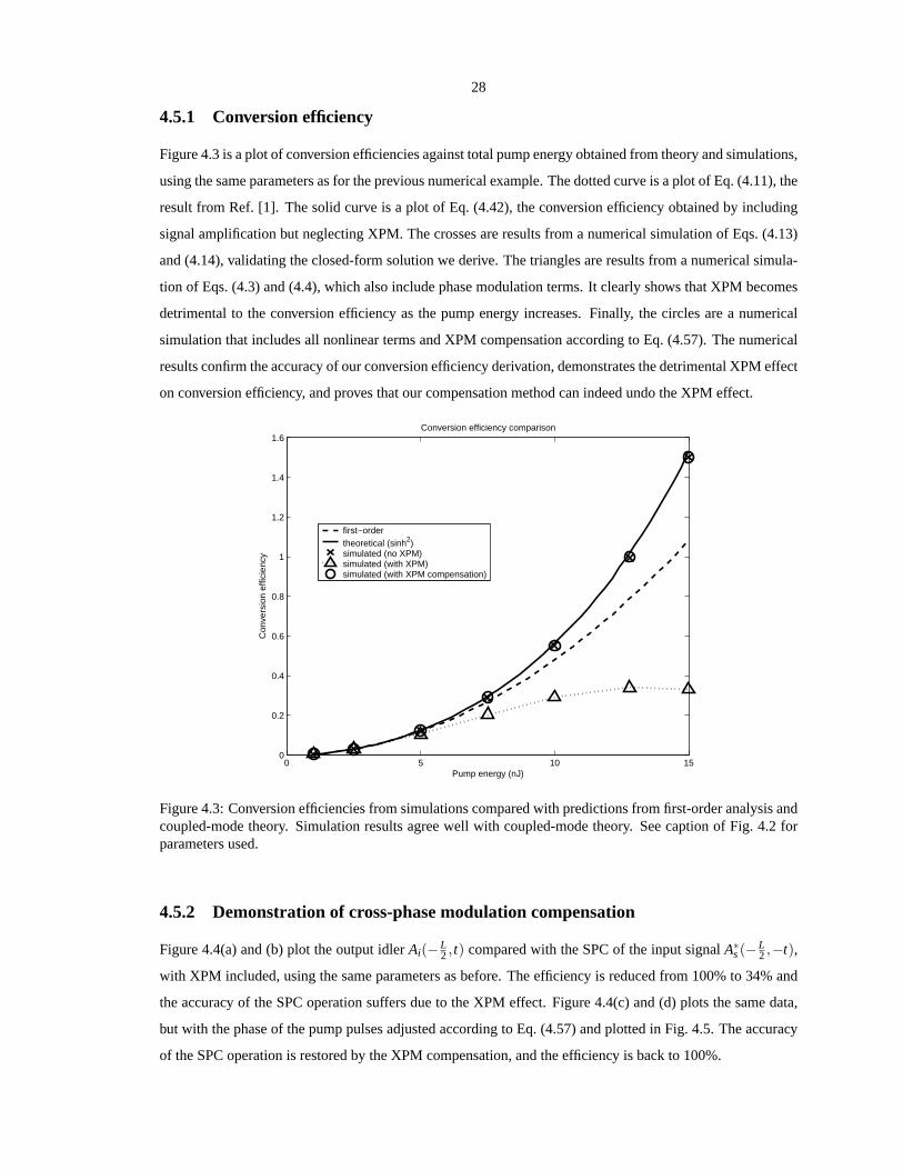
4.3 Conversion efficiencies from simulations compared withpredictions from first-order analy-
sis and coupled-mode theory. Simulation results agree wellwith coupled-mode theory. See
caption of Fig. 4.2 for parameters used. . . . . . . . . . . . . . . . . .. . . . . . . . . . . . 28

xi
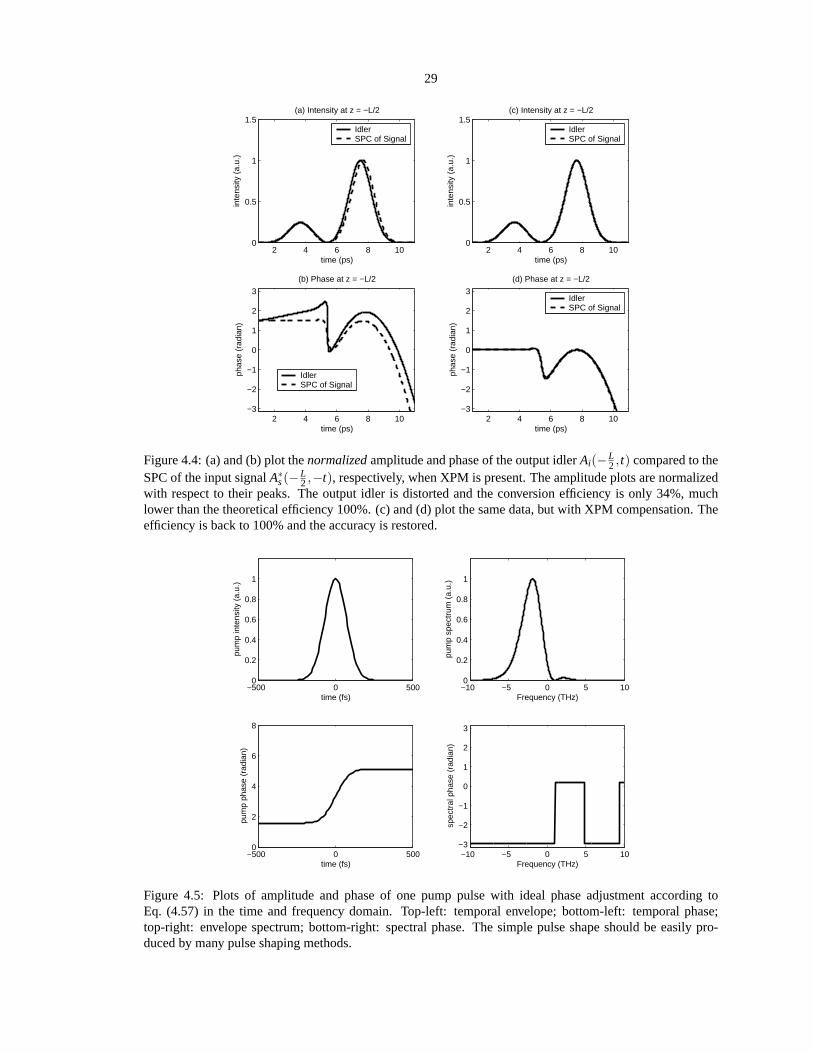
4.4 (a) and (b) plot thenormalizedamplitude and phase of the output idlerAi(−L2 , t) compared to
the SPC of the input signalA∗s(−L
2 ,−t), respectively, when XPM is present. The amplitude
plots are normalized with respect to their peaks. The outputidler is distorted and the conversion
efficiency is only 34%, much lower than the theoretical efficiency 100%. (c) and (d) plot the
same data, but with XPM compensation. The efficiency is back to 100% and the accuracy is
restored. . . . . . . . . . . . . . . . . . . . . . . . . . . . . . . . . . . . . . . . . . .. . . . 29
4.5 Plots of amplitude and phase of one pump pulse with ideal phase adjustment according to
Eq. (4.57) in the time and frequency domain. Top-left: temporal envelope; bottom-left: tempo-
ral phase; top-right: envelope spectrum; bottom-right: spectral phase. The simple pulse shape
should be easily produced by many pulse shaping methods. . . .. . . . . . . . . . . . . . . . 29
4.6 Amplitude and phase of output idler and input signal for the wave mixing process, with a signal
energy of 5 nJ, much above the pump depletion limit, to demonstrate the effect of pump depletion. 31
5.1 Geometry of SPC by quasi-phase-matched three-wave mixing. As(t) is the incoming signal
pulse with a carrier frequencyω0, andAp(t) is the second-harmonic pump pulse.Ai(t) is the
generated idler pulse. Quasi-phase matching is achieved bya χ(2) grating with periodΛ alongx. 34
5.2 Plots of intensity and phase of incoming signal and output idler from numerical analysis. It is
clear from the plots that the idler is a phase-conjugated andtime-reversed replica of the signal,
confirming our theoretical derivations. Parameters used areχ(2) = 50 pm/V,n0 = 3, L = 1 mm,
d = 5 µm, width iny = d, Ep = 2.1 µJ, pump fluence= EpLd . For such dimensions waveguide
confinement of the signal and the idler is necessary. . . . . . . .. . . . . . . . . . . . . . . . 38
5.3 Theoretical conversion efficiency derived from Eq. (5.17) and that from numerical analysis
plotted against pump energy. See caption of Fig. 5.2 for parameters used. . . . . . . . . . . . 39
6.1 Spontaneous SPC by TWM. . . . . . . . . . . . . . . . . . . . . . . . . . . . . .. . . . . . 43
6.2 Spontaneous SPC by FWM. . . . . . . . . . . . . . . . . . . . . . . . . . . . . .. . . . . . 43
7.1 Schematic of spectral phase conjugation (SPC) via type-II extended phase matching (EPM).
The signal and idler pulses, in orthogonal polarizations, have carrier frequencies ofωs andωi ,
while the pump pulse has a carrier frequency ofωp = ωs+ ωi . The EPM condition requires
that the signal and the idler counterpropagate with respectto the pump, which should be much
shorter than the input signal. . . . . . . . . . . . . . . . . . . . . . . . . .. . . . . . . . . . 54
7.2 Normalized polesp∞/(χAp0) plotted againstG, obtained by numerically solving Eq. (32),
indicating the onset of spatial instability beyond the thresholdG > π/2. More poles appear as
G is increased. . . . . . . . . . . . . . . . . . . . . . . . . . . . . . . . . . . . . . . .. . . 59
xii
7.3 Plots of intensity and phase of input signal, output signal, and output idler, from numerical
analysis of Eqs. (5) and (6). Parameters used arek′p = 1/(1.5× 108ms−1), k′s = 1.025k′p,
ki = 0.975k′p, Tp = 100 fs,Ts = 2 ps,L = 10 cm,ts = 4Ts, beam diameter = 200µm, As0 =
0.5exp[−(t − 2Ts)2/(2T2
s )]− exp[−(1+ 0.5 j)(t + 2Ts)2/(2T2
s )], Ap0 = exp[−t2/(2T2p )], and
G = π/4. The plots clearly show that the idler is the time-reversedand phase-conjugated
replica, i.e., SPC, of the signal. . . . . . . . . . . . . . . . . . . . . . .. . . . . . . . . . . . 62
7.4 Signal gainη + 1 and idler gainη versusG from numerical analysis compared with theory.
See caption of Fig. 3 for parameters used. . . . . . . . . . . . . . . . .. . . . . . . . . . . . 62
7.5 Plot of numerical idler gainη in dB againstG for L = 10 cm (solid) andL = 1 cm (dash-
dot), compared with the Fourier theory (dash), tan2(G) in dB. Three distinct regimes can be
observed for theL = 10 cm case; the moderate gain regime where the Fourier theoryis accurate,
the unstable regime where the gain increases exponentially, and the oscillation regime where
significant pump depletion occurs. ForL = 1 cm, the medium is not long enough for oscillation
to occur in the parameter range of interest. . . . . . . . . . . . . . .. . . . . . . . . . . . . . 63
8.1 Two-dimensional sketches of the two-photon probability amplitude before and after one of the
photons is time-reversed. Uncertainty in arrival time difference is transformed to uncertainty
in mean arrival time. . . . . . . . . . . . . . . . . . . . . . . . . . . . . . . . . .. . . . . . 73
8.2 A quantum temporal imaging system for quantum-enhancedclock synchronization. . . . . . . 74
8.3 The quantum destructive interference via a coupler is determined by the overlap (dark grey
area) of the two-photon amplitudeψ12(0, t,0, t ′) with its mirror image with respect to thet + t ′
axis,ψ12(0, t ′,0, t). . . . . . . . . . . . . . . . . . . . . . . . . . . . . . . . . . . . . . . . . 76
8.4 Quantum dispersive spreading of mean arrival time of a two-photon vector soliton. The cross-
phase modulation effect only preserves the two-photon coherence time, giving rise to temporal
entanglement with positive time correlation. One can also manipulate the coherence time in-
dependently by adiabatically changing the nonlinear coefficient along the propagation axis. . . 81
9.1 Proposed setup of generating multiphoton states with quantum-enhanced mean position ac-
curacy via adiabatic control of vector solitons. A pulse is coupled into a vector soliton in a
multimode nonlinear waveguide, in which dispersion adiabatically increases or the Kerr non-
linearity adiabatically decreases. A second waveguide with an opposite dispersion is used for
compensating the quantum dispersive spreading of the mean position. . . . . . . . . . . . . . 88
10.1 First row: schematics of the spatial quantum enhancement setup via adiabatic soliton expan-
sion. Second row: sketches of the spatial probability amplitude,ψ(x1,x2), for an example of
two photons in each step of the process. Third row: sketches of the momentum probability
amplitude,φ(k1,k2). Consult text for details of each step of the process. . . . . . .. . . . . . 101

xiii
11.1 Reflectionless evanescent wave amplification (REWA) bytwo slab waveguides, wheren1 > n0. 106
12.1 Intensity (left column), phase (middle column), and phase gradient (right column) of two opti-
cal vortex solitons with the same charge (top row), which should rotate in the same sense, and
those of two vortex solitons with opposite charges, which should drift in a direction perpendic-
ular to their separation. The phase gradient near the centers of the vortices is not plotted due to
its divergence. . . . . . . . . . . . . . . . . . . . . . . . . . . . . . . . . . . . . .. . . . . . 118
12.2 Sketches of velocity and flux of a vortex blob and an optical vortex along a line across the
center, to illustrate the similarities between the two in terms of the flux. . . . . . . . . . . . . 120
12.3 Comparison between a viscous boundary layer and an optical boundary layer. . . . . . . . . . 123
12.4 Setup of numerical experiment (not to scale). . . . . . . . .. . . . . . . . . . . . . . . . . . 124
12.5 The intensity of the optical beam at a normalized propagation distanceζ = 10, for M = 0.4
andR = 12.8. The dark ellipse is the low-refractive-index region thatacts as an impenetrable
object. Optical vortex solitons are seen to be created on thetop and bottom side of the ellipse,
While the convection of the solitons behind the object resembles the twin vortices behind an
obstacle in a viscous fluid flow. . . . . . . . . . . . . . . . . . . . . . . . . .. . . . . . . . . 124
12.6 A vector plot of the fluxJ atζ = 10, forM = 0.4 andR = 12.8, which confirms the similarity
between the numerically observed dynamics and the phenomenon of twin vortices. . . . . . . 125
12.7 A plot of the momentum vorticity∇× J at ζ = 10, forM = 0.4 andR = 12.8. A white dot
indicates that the vortex has a positive topological chargeand a black dot indicates that the
vortex has a negative charge. The plot shows the similarity between the numerically observed
dynamics and the phenomenon of twin vortices. . . . . . . . . . . . .. . . . . . . . . . . . . 125
12.8 The intensity of the optical beam at a normalized propagation distanceζ = 20, for M = 0.4
andR = 12.8. The qualitative dynamical behavior is essentially unchanged from that shown
in Fig. 12.5. . . . . . . . . . . . . . . . . . . . . . . . . . . . . . . . . . . . . . . . .. . . . 126
12.9 A vector plot of the fluxJ at ζ = 20, forM = 0.4 andR = 12.8. . . . . . . . . . . . . . . . 126
12.10 A plot of the momentum vorticity∇×J at ζ = 20, forM = 0.4 andR = 12.8. . . . . . . . . 126
12.11 The optical intensity atζ = 10, forM = 0.4 andR = 25.6. The vortex solitons are observed
to be smaller, and the phenomenon of twin vortices is again observed. . . . . . . . . . . . . . 127
12.12 The fluxJ at ζ = 10, forM = 0.4 andR = 25.6. . . . . . . . . . . . . . . . . . . . . . . . 127
12.13 The momentum vorticity∇×J at ζ = 10, forM = 0.4 andR = 25.6. . . . . . . . . . . . . 127
12.14 Optical intensity atζ = 20, for M = 0.4 andR = 25.6. The twin vortices become unstable
and detach alternatively from the object. . . . . . . . . . . . . . . .. . . . . . . . . . . . . . 128
12.15 Flux atζ = 20, forM = 0.4 andR = 25.6, which shows a flow pattern strongly resembling
the Karman vortex street. . . . . . . . . . . . . . . . . . . . . . . . . . . . . . . . . . . . .. 128
xiv
12.16 Vorticity atζ = 20, forM = 0.4 andR = 25.6, which confirms that the alternate bunches of
vortices indeed have the right charges that resemble the Karman vortex street phenomenon. . . 129
12.17 Sketch of a split-step optical system that approximates the ideal nonlinear medium. . . . . . . 131

xv
List of Tables
3.1 Comparison of TPC and SPC in terms of propagation effectsthat can be compensated by each
scheme. EOD stands for even-order dispersion, OOD stands for odd-order dispersion, SPM
stands for self-phase modulation, SS stands for self-steepening, and IRS stands for intrapulse
Raman scattering. . . . . . . . . . . . . . . . . . . . . . . . . . . . . . . . . . . .. . . . . 14
1
Chapter 1
Summary
This thesis investigates various classical and quantum optics techniques for applications in optical communi-
cations, quantum information processing, imaging, and computing.
Chapter 2 presents a numerical technique for reversing femtosecond pulse propagation in an optical fiber,
such that given any output pulse it is possible to obtain the input pulse shape by numerically undoing all
dispersion and nonlinear effects. The technique is tested against experimental results, and it is shown that it
can be used for fiber output pulse optimization in both the anomalous and normal dispersion regimes [1].
Chapter 3 proposes the use of spectral phase conjugation to compensate for dispersion of all orders, self-
phase modulation, and self-steepening of an optical pulse in a fiber. Although this method cannot compensate
for loss and intrapulse Raman scattering, it is superior to the previously suggested midway temporal phase
conjugation method if high-order dispersion is a main source of distortion. The reshaping performance of
our proposed scheme and a combined temporal and spectral phase conjugation scheme in the presence of
uncompensated effects is studied numerically [2].
Chapter 4 analyzes spectral phase conjugation with short pump pulses in a third-order nonlinear material
in depth. It is shown that if signal amplification is considered, the conversion efficiency can be significantly
higher than previously considered, while the spectral phase conjugation operation remains accurate. A novel
method of compensating for cross-phase modulation, the main parasitic effect, is also proposed. The validity
of our theory and the performance of the spectral phase conjugation scheme are studied numerically [3].
Chapter 5 proposes a novel spectral phase conjugation scheme by three-wave mixing. It is shown that
a phase-conjugated and time-reversed replica of the incoming signal can be generated, if appropriate quasi-
phase matching is achieved and the three-wave mixing process is transversely pumped by a short second-
harmonic pulse [4].
Chapter 6 studies spontaneous parametric processes pumpedtransversely with short pulses under a uni-
fied framework, which proves that such processes can efficiently generate entangled photon pairs with time
anticorrelation and frequency correlation. Improvementsupon previously proposed schemes can be made by
the use of quasi-phase matching, four-wave mixing, and cross-phase modulation compensation. The use of
frequency-correlated photons in the Hung-Ou-Mandel interferometer is also studied [5].

2
Chapter 7 demonstrates that the copropagating three-wave-mixing parametric process, with appropriate
type-II extended phase matching and pumped with a short second-harmonic pulse, can perform spectral phase
conjugation and parametric amplification, which shows a threshold behavior analogous to backward wave
oscillation. The process is also analyzed in the Heisenbergpicture, which predicts a spontaneous parametric
down conversion rate in agreement with experimental results reported elsewhere [6].
Chapter 8 derives the equations that govern the temporal evolution of two photons in the Schrodinger
picture, taking into account the effects of loss, group-velocity dispersion, temporal phase modulation, linear
coupling among different optical modes, and four-wave mixing. Inspired by the formalism, the concept
of quantum temporal imaging is proposed, which uses dispersive elements and temporal phase modulators
to manipulate the temporal correlation of two entangled photons. The exact solution of a two-photon vector
soliton is also presented, in order to demonstrate the ease of use and intuitiveness of the proposed formulation
[7].
Chapter 9 shows that optical pulses with a mean position accuracy beyond the standard quantum limit
can be produced by adiabatically expanding an optical vector soliton followed by classical dispersion man-
agement. The proposed scheme is also capable of entangling positions of optical pulses and can potentially
be used for general continuous-variable quantum information processing [8].
Chapter 10 studies spatial quantum enhancement effects under a unified framework. An approach of
generating arbitrary quantum lithographic patterns by theuse of multiphoton coincident momentum states is
proposed. It is shown that the multiphoton absorption rate of photons with a quantum-enhanced lithographic
resolution is reduced, not enhanced, contrary to popular belief. Finally, the use of adiabatic soliton expansion
followed by negative refraction is proposed to beat both thestandard quantum limit on the optical beam
displacement accuracy, as well as that on the minimum spot size of quantum lithography [9].
In Chapter 11, utilizing the underlying physics of evanescent wave amplification by a negative-refractive-
index slab, it is shown that evanescent waves with specific spatial frequencies can also be amplified without
any reflection simply by two dielectric planar waveguides. The simple configuration allows one to take
advantage of the high resolution limit of a high-refractive-index material without contact with the object [10].
Chapter 12 presents theoretical and numerical evidence to show that self-defocusing nonlinear optical
propagation can be used to compute Euler fluid dynamics and possibly Navier-Stokes fluid dynamics. In
particular, the formation of twin vortices and the Karman vortex street behind an obstacle, two well-known
viscous fluid phenomena, is numerically demonstrated usingthe nonlinear Schrodinger equation [11].

3
Bibliography
[1] M. Tsang, D. Psaltis, and F. G. Omenetto, Opt. Lett.28, 1873 (2003).
[2] M. Tsang and D. Psaltis, Opt. Lett.28, 1558 (2003).
[3] M. Tsang and D. Psaltis, Opt. Express12, 2207 (2004).
[4] M. Tsang and D. Psaltis, Opt. Commun.242, 659 (2004).
[5] M. Tsang and D. Psaltis, Phys. Rev. A71, 043806 (2005).
[6] M. Tsang, J. Opt. Soc. Am. B23, 861 (2006).
[7] M. Tsang and D. Psaltis, Phys. Rev. A73, 013822 (2006).
[8] M. Tsang, e-print quant-ph/0603088 [submitted to Phys.Rev. Lett. ].
[9] M. Tsang, under preparation.
[10] M. Tsang and D. Psaltis, e-print physics/0603079 [submitted to Opt. Lett. ].
[11] M. Tsang and D. Psaltis, under preparation.
4
Chapter 2
Reverse propagation of femtosecondpulses in optical fibers
2.1 Introduction
Dispersion and nonlinear effects have been the bottleneck of ultrafast pulse propagation in an optical fiber.
Various schemes, for example, optical solitons [1] and optical phase conjugation (OPC) [2, 3] have been pro-
posed to compensate for these effects, yet the high-order distortions including third-order dispersion (TOD),
self-steepening, and Raman scattering remain undefeated.Femtosecond power delivery in a normally dis-
persive fiber, which is useful for biomedical applications,is especially difficult to achieve because normal
dispersion and nonlinear effects always tend to broaden anddistort a pulse. Another scheme is to embrace
all the effects and adopt an adaptive optimization method, typically in the form of genetic algorithm, hoping
that modulating the input pulse shape can produce an output with desirable properties [4, 5, 6]. Although
an adaptive method can compensate for pulse propagation distortions and unknown experimental variables,
it does not make full use of our theoretical knowledge of optical fiber ultrafast pulse propagation and may
therefore be time consuming and suboptimal.
In this chapter we show that by reversing the nonlinear pulsepropagation equation it is possible to theo-
retically predict the exact input pulse shape that gives a desired output of a fiber. All dispersion and nonlinear
effects can be incorporated into the simulation, and hence one can produce any kind of pulse shape at the
output end by shaping the input pulse appropriately according to the calculated result. In conjunction with
currently available femtosecond pulse-shaping techniques such as 4f pulse shaping [7] this approach is espe-
cially suited to provide custom-shaped high-power ultrafast pulse delivery both in normally and anomalously
dispersive fibers.

5
2.2 Theory
The nonlinear pulse propagation equation in a fiber is given by the general form [1]
∂A(z,T)
∂z= D+ N[A(z,T)]A(z,T), (2.1)
whereA(z,T) is the pulse envelope,D is the linear operator that includes absorption and all dispersion effects,
andN is the nonlinear operator that includes all nonlinear effects and is a function ofA(z,T). Mathematically,
the output is obtained by application of the propagation operator to the input:
A(L,T) = exp
LD+∫ L
0N[A(z,T)]dz
A(0,T), (2.2)
whereL is the length of the fiber. The input can also be expressed in terms of the output by application of the
reverse propagation operator:
A(0,T) = exp
−LD−∫ L
0N[A(z,T)]dz
A(L,T). (2.3)
To solve this equation and derive the input pulse shape giventhe output, we use the standard Fourier split-step
method:
A(z,T) ≈ exp(−hD)exp−hN[A(z+h,T)]A(z+h,T), (2.4)
in each step of which the linear and nonlinear effects on a pulse shape are evaluated separately for a small
propagation distanceh.
Figure 2.1: Comparison of OPC and reverse propagation.
As a comparison, let us consider the OPC technique in the operator notation. Figure 2.1 depicts schemat-
ically the OPC method and the reverse propagation method. Byconjugating Eq. (2.2) and comparing the
result with Eq. (2.3), one can see that OPC can reconstruct aninput pulse ifD and N contain operators
with the propertyM = −M∗. This restriction precludes many important phenomena, such as loss, TOD, and

6
self-steepening, that may severely hamper the accuracy of pulse reconstruction by OPC, especially in the
femtosecond regime. In a numerical simulation of reverse propagation, however, there is no such limitation,
and all effects can be included to yield the optimal input pulse shape.
To model femtosecond pulse propagation, we choose the linear operatorD to be
D = −α2− j
β2
2∂ 2
∂T2 +β3
6∂ 3
∂T3 . (2.5)
The first term corresponds to loss, the second term corresponds to group-velocity dispersion (GVD), and the
third term corresponds to TOD. The higher-order dispersionterms are neglected because of the relatively
short length considered here but can be easily included if the need arises.
The nonlinear operatorN is
N = jγ[
|A|2 +j
ω0
1A
∂∂T
(|A|2A)−TR∂ |A|2∂T
]
. (2.6)
The first term corresponds to optical Kerr effect, the secondterm corresponds to self-steepening, and the third
term corresponds to intrapulse Raman scattering.
Figure 2.2: Reverse propagation of an experimental output pulse. The experimental output pulse shape isplotted atz= 0 m and numerically propagates in reverse fromz= 0 m toz= −10 m.
2.3 Comparison with experiments
To test the validity of reverse propagation, in an experiment we launch a 150 fs positively chirped hyperbolic
secant pulse with a peak power of 1 kW in a 10 m long Corning SMF-28 fiber [6]. From frequency-resolved
7
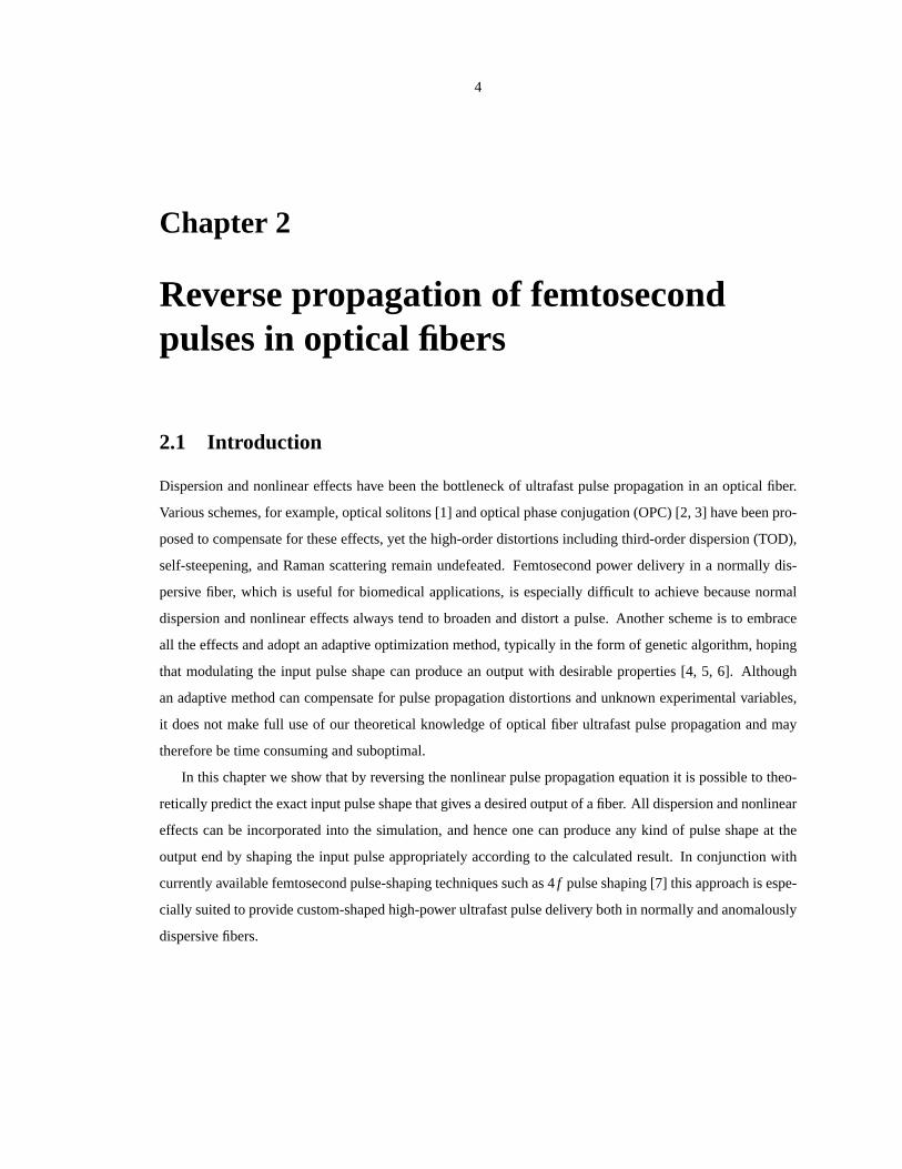
optical gating measurements we obtain the amplitude and phase of both input and output pulses. The output
pulse is then reverse propagated in a computer simulation asin Fig. 2.2. The output pulse shape is plotted at
z= 0 m at the top of the graph, and propagation effects are reversed numerically as the pulse goes fromz= 0
m to z= −10 m. The simulated input from reverse propagation is compared with the experimental input in
Fig. 2.3. Both pulses are remarkably similar, with nearly identical amplitudes and positive chirp, showing
that the reverse propagation theory is consistent with experimental results.
Figure 2.3: Comparison of the input obtained from reverse propagation and the actual experimental input.
2.4 Numerical analysis
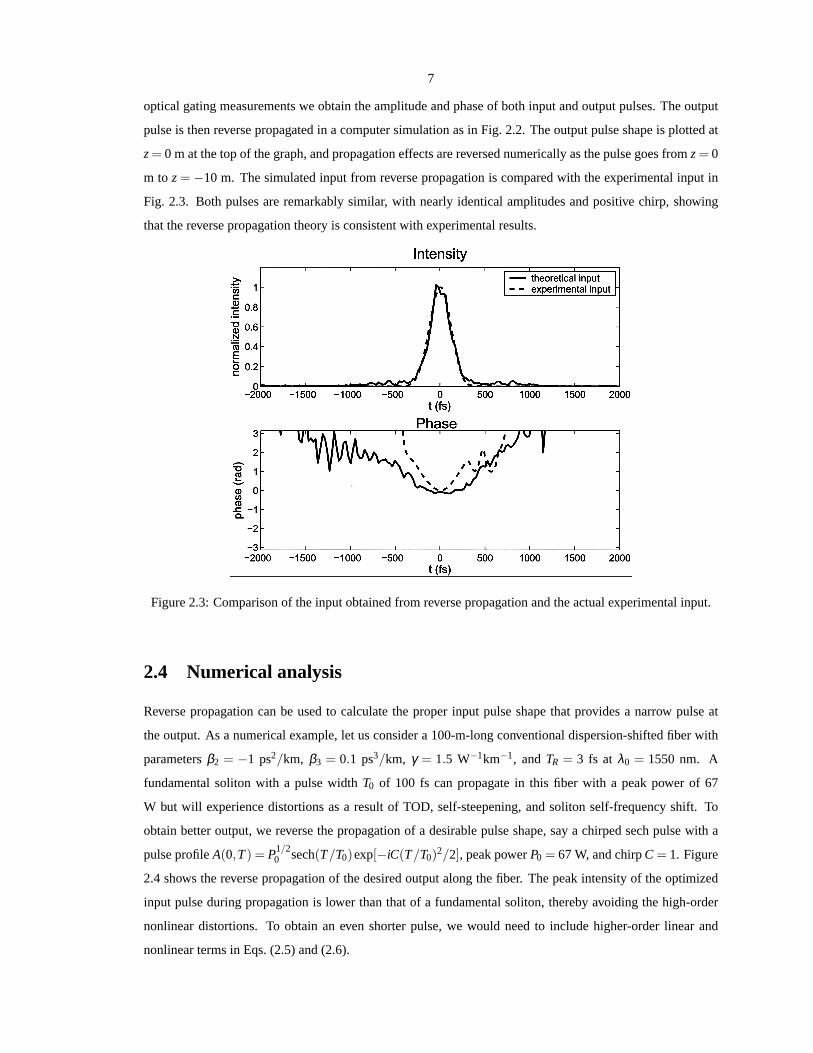
Reverse propagation can be used to calculate the proper input pulse shape that provides a narrow pulse at
the output. As a numerical example, let us consider a 100-m-long conventional dispersion-shifted fiber with
parametersβ2 = −1 ps2/km, β3 = 0.1 ps3/km, γ = 1.5 W−1km−1, andTR = 3 fs at λ0 = 1550 nm. A
fundamental soliton with a pulse widthT0 of 100 fs can propagate in this fiber with a peak power of 67
W but will experience distortions as a result of TOD, self-steepening, and soliton self-frequency shift. To
obtain better output, we reverse the propagation of a desirable pulse shape, say a chirped sech pulse with a
pulse profileA(0,T) = P1/20 sech(T/T0)exp[−iC(T/T0)
2/2], peak powerP0 = 67 W, and chirpC = 1. Figure
2.4 shows the reverse propagation of the desired output along the fiber. The peak intensity of the optimized
input pulse during propagation is lower than that of a fundamental soliton, thereby avoiding the high-order
nonlinear distortions. To obtain an even shorter pulse, we would need to include higher-order linear and
nonlinear terms in Eqs. (2.5) and (2.6).
8
Figure 2.4: Reverse propagation of a chirped sech pulse atλ0 = 1550 nm.
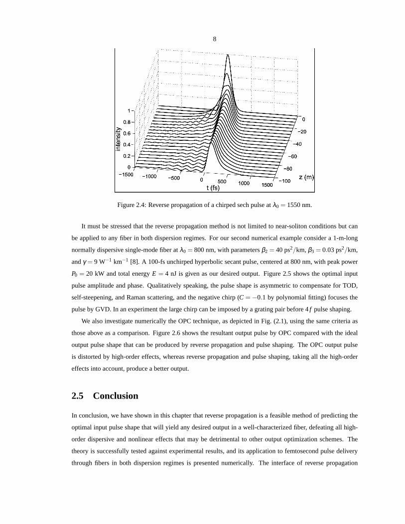
It must be stressed that the reverse propagation method is not limited to near-soliton conditions but can
be applied to any fiber in both dispersion regimes. For our second numerical example consider a 1-m-long
normally dispersive single-mode fiber atλ0 = 800 nm, with parametersβ2 = 40 ps2/km, β3 = 0.03 ps2/km,
andγ = 9 W−1 km−1 [8]. A 100-fs unchirped hyperbolic secant pulse, centered at 800 nm, with peak power
P0 = 20 kW and total energyE = 4 nJ is given as our desired output. Figure 2.5 shows the optimal input
pulse amplitude and phase. Qualitatively speaking, the pulse shape is asymmetric to compensate for TOD,
self-steepening, and Raman scattering, and the negative chirp (C = −0.1 by polynomial fitting) focuses the
pulse by GVD. In an experiment the large chirp can be imposed by a grating pair before 4f pulse shaping.
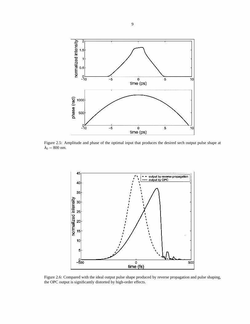
We also investigate numerically the OPC technique, as depicted in Fig. (2.1), using the same criteria as
those above as a comparison. Figure 2.6 shows the resultant output pulse by OPC compared with the ideal
output pulse shape that can be produced by reverse propagation and pulse shaping. The OPC output pulse
is distorted by high-order effects, whereas reverse propagation and pulse shaping, taking all the high-order
effects into account, produce a better output.
2.5 Conclusion
In conclusion, we have shown in this chapter that reverse propagation is a feasible method of predicting the
optimal input pulse shape that will yield any desired outputin a well-characterized fiber, defeating all high-
order dispersive and nonlinear effects that may be detrimental to other output optimization schemes. The
theory is successfully tested against experimental results, and its application to femtosecond pulse delivery
through fibers in both dispersion regimes is presented numerically. The interface of reverse propagation
9
Figure 2.5: Amplitude and phase of the optimal input that produces the desired sech output pulse shape atλ0 = 800 nm.
Figure 2.6: Compared with the ideal output pulse shape produced by reverse propagation and pulse shaping,the OPC output is significantly distorted by high-order effects.

10
code to a pulse shaper can be envisaged for short propagationlengths, so that the proper modulation is
applied to the input pulse by the programmable optical modulator of choice. For longer distances, practical
realizations become more complex as linear distortions become too large to be overcome by the available
modulators alone. In this case linear compensators can be combined with programmable modulators and
reverse propagation predictions to compensate for all distortions.
11
Bibliography
[1] G. P. Agrawal,Nonlinear Fiber Optics(Academic, San Diego, Calif., 2001).
[2] A. Yariv, D. Fekete, and D. M. Pepper, Opt. Lett.4, 52 (1979).
[3] R. A. Fisher, B. R. Suydam, and D. Yevick, Opt. Lett.8, 611 (1983).
[4] R. S. Judson and H. Rabitz, Phys. Rev. Lett.68, 1500 (1992).
[5] F. G. Omenetto, B. P. Luce, and A. J. Taylor, J. Opt. Soc. Am. B 16, 2005 (1999).
[6] F. G. Omenetto, A. J. Taylor, M. D. Moores, and D. H. Reitze, Opt. Lett.26, 938 (2001).
[7] A. M. Weiner, J. P. Heritage, and E. M. Kirschner, J. Opt. Soc. Am. B5, 1563 (1988).
[8] S. W. Clark, F. O. Ilday, and F. W. Wise, Opt. Lett.26, 1320 (2001).
12
Chapter 3
Dispersion and nonlinearitycompensation via spectral phaseconjugation
3.1 Introduction
Temporal phase conjugation (TPC) was proposed to compensate for group-velocity dispersion [1], self-phase
modulation [2], and intrapulse Raman scattering [3] of an optical pulse in a fiber. However, when the pulse
width is sufficiently short or the center wavelength is near the zero-dispersion point, third-order dispersion and
self-steepening effects become more prominent and limit the reshaping performance of TPC. To compensate
for the high-order effects, alternative methods [4, 5, 6, 7]have been suggested, but many of them are either
too complicated or are only able to compensate for a limited number of propagation effects. An interesting
scheme, which compensates for all effects by both TPC and a suitably chosen dispersion map, is also proposed
by Pinaet al. [8].
TPCA(0,T) A(L,T) A*(L,T) A*(0,T)Fiber Fiber
SPCA(0,T) A(L,T) A*(L,-T) A*(0,-T)Fiber Fiber
Figure 3.1: Schematics of TPC and SPC.
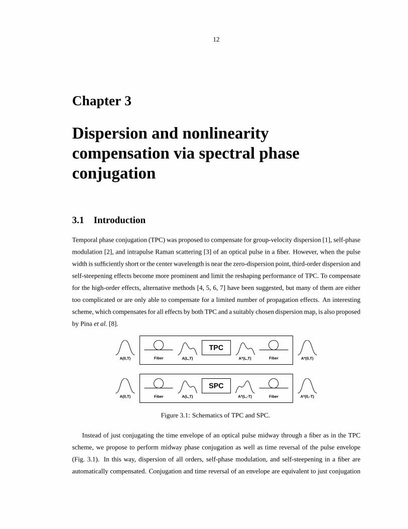
Instead of just conjugating the time envelope of an optical pulse midway through a fiber as in the TPC
scheme, we propose to perform midway phase conjugation as well as time reversal of the pulse envelope
(Fig. 3.1). In this way, dispersion of all orders, self-phase modulation, and self-steepening in a fiber are
automatically compensated. Conjugation and time reversalof an envelope are equivalent to just conjugation
13
of the optical pulse in the frequency domain, hence the name spectral phase conjugation (SPC).
3.2 Theory
Consider a pulseE(t) = A(t)exp(− jω0t) with envelopeA(t) and center frequencyω0. If we take the conju-
gate of the Fourier transform ofE(t), it becomes
E∗(ω) =[
∫ ∞
−∞A(t)exp(− jω0t)exp( jωt)dt
]∗(3.1)
=∫ ∞
−∞A∗(−t)exp(− jω0t)exp( jωt)dt (3.2)
where the substitutiont → −t is made. Hence, conjugation of individual spectral components of a pulse
is equivalent to phase conjugation and time reversal of the temporal envelope. TPC, on the other hand,
corresponds to conjugation and inversion in the frequency domain.
Midway SPC is unique in the sense that it can compensate for all dispersion and most nonlinearities
simultaneously. Consider the general pulse propagation equation in a fiber,
∂A(z,T)
∂z=[
DT + NT(
A(z,T))
]
A(z,T), (3.3)
wherez is the propagation distance,T is the retarded time with respect to the group velocity 1/β1 of the pulse
(T = t −β1z), andA(z,T) is the pulse envelope.DT is the linear operator,
DT = −α2
+∞
∑n=2
jβn
n!( j
∂∂T
)n, (3.4)
where the first term on the right-hand side is the loss term, and the remaining terms arenth-order dispersion
terms.NT is the nonlinear operator, which can be expressed as the following for a femtosecond pulse,
NT(A) = jγ[
|A|2 +j
ω0
1A
∂∂T
(|A|2A)−TR∂ |A|2∂T
]
, (3.5)
where the first term on the right-hand side is the self-phase modulation term, the second term is self-
steepening, and the third term is intrapulse Raman scattering [9]. The subscriptT of DT and NT denotes
the derivatives with respect toT in the operators.
We rewrite Eq. (3.3) to express the output pulse in terms of the propagation operator applied to the input
pulse [9],
A(L,T) = exp[
LDT +
∫ L
0NT(
A(z,T))
dz]
A(0,T), (3.6)
whereL is the fiber length. The input can also be expressed in terms ofthe output by applying the reverse
14
propagation operator [7],
A(0,T) = exp[
−LDT −∫ L
0NT(
A(z,T))
dz]
A(L,T). (3.7)
Now let us take the complex conjugate of Eq. (3.7) and make thesubstitutionT →−T. Eq. (3.7) becomes
A∗(0,−T) = exp[
−LD∗−T −
∫ L
0N∗−T
(
A(z,−T))
dz]
A∗(L,−T). (3.8)
The conjugated and time reversed linear operator, ignoringloss, is
D∗−T =
∞
∑n=2
− jβn
n![(− j)(− ∂
∂T)]n (3.9)
=∞
∑n=2
− jβn
n!( j
∂∂T
)n = −DT . (3.10)
Similarly, the nonlinear operator, ignoring intrapulse Raman scattering, is
N∗−T(A(z,−T)) = −NT(A∗(z,−T)). (3.11)
In general, we only keep terms that acquire a minus sign when conjugation and time reversal are both ap-
plied. All operator terms, except loss and intrapulse Ramanscattering, satisfy our criteria due to their odd
combinations ofj ’s and time derivatives. With the substitutionz→ L−z′, Eq. (3.8) becomes
A∗(0,−T) = exp[
LDT +∫ L
0NT(
A∗(L−z′,−T))
dz′]
A∗(L,−T). (3.12)
Eq. (3.12) has the exact same form as Eq. (3.6), but withA∗(L− z′,−T) as the solution. In other words, if
we launchA∗(L,−T) in another identical fiber, the final outputA∗(0,−T) is a conjugated and time reversed
version of the first input. This result can only be applied to cases where loss and intrapulse Raman scattering
can be neglected. Table 3.1 summarizes the propagation effects that can be compensated by TPC and SPC,
respectively.
loss EOD OOD SPM SS IRSTPC × √ × √ × √
SPC × √ √ √ √ ×
Table 3.1: Comparison of TPC and SPC in terms of propagation effects that can be compensated by eachscheme. EOD stands for even-order dispersion, OOD stands for odd-order dispersion, SPM stands for self-phase modulation, SS stands for self-steepening, and IRS stands for intrapulse Raman scattering.

15
To identify important propagation effects for a given optical pulse transmission system, it is useful to
define a characteristic length for each propagation effect [9],
Lloss = loss length= 1/α, (3.13)
LD = dispersion length= T20 /|β2|, (3.14)
L′D = third-order dispersion length= T3
0 /|β3|, (3.15)
LNL = nonlinear length= 1/(γP0), (3.16)
LSS = self-steepening length= ω0T0/(γP0), (3.17)
LR = Raman length= T0/(TRγP0), (3.18)
whereT0 is the pulse width. The significance of a propagation effect can be roughly estimated by the ratio
of the total propagation distanceLtotal to the characteristic length. Hence a phase conjugation system should
be designed such that the characteristic lengths of uncompensated propagation effects are much longer than
Ltotal. This is demonstrated next in the numerical simulations.
3.3 Numerical analysis
As a numerical example, considerλ0 = 1550 nm, two dispersion-shifted fibers, each with lengthLtotal/2 = 1
km, parametersβ2 = −1 ps2/km, β3 = 0.1 ps3/km, γ = 1.5 W−1km−1, α = 0.2 dB/km,TR = 3 fs, a temporal
or spectral phase conjugator in the middle, an amplifier at each fiber end to compensate for loss, and a super-
Gaussian input pulse,
A(t) =√
P0exp[−12(
TT0
)6], (3.19)
with T0 = 200 fs, and peak powerP0 = 1.7 W. The peak power is chosen to be one-tenth of that of a funda-
mental soliton, such thatLloss = 2 km,LD = 0.04 km,L′D = 0.08 km, andLNL = 0.4 km. Other characteristic
lengths are too long to be significant. SinceLNL is comparable toLtotal while much longer than the dispersion
lengths, we expect nonlinear effects to be observable but less significant than dispersion effects. The output
pulses with and without compensation schemes are plotted inFig. 3.2. SPC reconstructs the input pulse at
the output almost perfectly, while the TPC output pulse is significantly distorted by third-order dispersion.
At this power level, SPC has the advantage over TPC for the former’s ability to compensate for all important
linear and nonlinear effects together with an amplifier.
In practice, SPC can be performed by spectral holography [4], short-pump four-wave mixing [10] or spec-
tral four-wave mixing [11]. If SPC is to be used in a communication system, one must perform time reversal
only on each time slot or a group of slots, within the time window of the SPC device. A synchronous clock,
in the form of pump pulses, will therefore be required, unfortunately. The pulses also need to be periodically
conjugated before they breach adjacent time windows. In this case solitons are preferred because their broad-

16
−500 −400 −300 −200 −100 0 100 200 300 400 5000
0.2
0.4
0.6
0.8
1
time (fs)
norm
aliz
ed in
tens
ity
inputuncompensatedTPCSPC
Figure 3.2: Input and output pulses with and without compensation schemes, when a 1.7 W 200 fs super-Gaussian pulse propagates for a total distance of 2 km.
ening is much slower than conventional pulses and the frequency of conjugation can be minimized. We note
that periodic conjugation is also required in other schemesfor different reasons, such as that suggested by
Pinaet. al., to satisfy the path-averaging assumption.
Since SPC can compensate for distortions not compensated byTPC, and vice versa, we propose that a
hybrid scheme combining SPC and TPC can offer superior performance. An example would be to sandwich
a temporal phase conjugator with two midway SPC systems, such that the Raman effect uncompensated in a
SPC system can be compensated by the TPC system, at least to first order. More rigorous analysis is required
to fully estimate the performance of a hybrid scheme.
Our second numerical example tests the compensation capabilities of SPC and the hybrid scheme for
multiple solitons. It has been suggested that TPC can compensate for soliton interactions [12]. Fig. 3.3 plots
the output pulses obtained from various compensation schemes for the same parameters as the first example,
but with a total length of 1 km and a 17 W alternativelyπ phase-shifted sech soliton train representing the
bit sequence 10110111. SPC undoes soliton interactions andpulse distortions better than TPC in this case,
while the hybrid scheme performs slightly better than SPC. This can be attributed to the fact that the hybrid
scheme has more phase conjugation stages for the same total length. The hybrid scheme, however, can also
compensate for the Raman-induced frequency shift, which cannot be compensated by SPC alone. The mean
frequency shift of the TPC output is calculated to be +0.032 THz, that of the SPC output is−0.16 THz, while
that of the hybrid scheme is only−0.027 THz.
17
−5000 −4000 −3000 −2000 −1000 0 1000 2000 3000 4000 50000
0.5
1
Inpu
t
−5000 −4000 −3000 −2000 −1000 0 1000 2000 3000 4000 50000
0.5
1
Unc
ompe
nsat
ed
−5000 −4000 −3000 −2000 −1000 0 1000 2000 3000 4000 50000
0.5
1T
PC
−5000 −4000 −3000 −2000 −1000 0 1000 2000 3000 4000 50000
0.5
1
SP
C
−5000 −4000 −3000 −2000 −1000 0 1000 2000 3000 4000 50000
0.5
1
time (fs)
TP
C+
SP
C
Figure 3.3: Input and output pulses with and without compensation schemes, when multiple 17 W 200 fssolitons propagates for a total distance of 1 km.
3.4 Conclusion
In conclusion, we have proven that SPC can compensate for allthe considered linear and nonlinear distortions
to optical pulses if loss and intrapulse Raman scattering can be neglected. Moreover, SPC and a hybrid
scheme combining TPC and SPC are both shown numerically to offer better compensation of pulse distortions
and soliton interactions than TPC for femtosecond pulses.
18
Bibliography
[1] A. Yariv, D. Fekete, and D. M. Pepper, Opt. Lett.4, 52 (1979).
[2] R. A. Fisher, B. R. Suydam, and D. Yevick, Opt. Lett.8, 611 (1983).
[3] S. Chi and S. F. Wen, Opt. Lett.19, 1705 (1994).
[4] A. M. Weiner, D. E. Leaird, D. H. Reitze, and E. G. Paek, IEEE J. Quantum Electron.28, 2251 (1992).
[5] C. Chang, H. P. Sardesai, and A. M. Weiner, Opt. Lett.23, 283 (1998).
[6] F. G. Omenetto, A. J. Taylor, M. D. Moores, and D. H. Reitze, Opt. Lett.26, 938 (2001).
[7] M. Tsang, D. Psaltis, and F. G. Omenetto, Opt. Lett.28, 1873 (2003).
[8] J. Pina, B. Abueva, and G. Goedde, Opt. Commun.176, 397 (2000).
[9] G. P. Agrawal,Nonlinear Fiber Optics(Academic Press, San Diego, 2001).
[10] D. A. B. Miller, Opt. Lett.5, 300 (1980).
[11] D. Marom, D. Panasenko, R. Rokitski, P. Sun, and Y. Fainman, Opt. Lett.25, 132 (2000).
[12] W. Forysiak and N. J. Doran, Electron. Lett.30, 154 (1994).
19
Chapter 4
Spectral phase conjugation withcross-phase modulation compensation
4.1 Introduction
Spectral phase conjugation (SPC) [1] is the phase conjugation of individual spectral components of an optical
waveform, which is equivalent to phase conjugation and timereversal of the pulse envelope. Joubertet al.
prove that midway SPC can compensate for all chromatic dispersion [2]. In the previous chapter we prove
that midway SPC can simultaneously compensate for self-phase modulation (SPM), self-steepening and dis-
persion [3]. The physical implementation of SPC is first suggested by Miller using short-pump four-wave
mixing (FWM) [1], and later demonstrated using photon echo [4, 5], spectral hole burning [6, 7], temporal
holography [2], spectral holography [8], and spectral three-wave mixing (TWM) [9]. The FWM scheme is es-
pecially appealing to real-world applications such as communications and ultrashort pulse delivery due to its
simple setup. However, low conversion efficiency and parasitic Kerr effects make a practical implementation
difficult.
In this chapter we derive an accurate expression for the output idler when the conversion efficiency,
defined as the output idler energy divided by the input signalenergy, is high. We prove that if signal ampli-
fication is considered, the SPC process remains intact and the conversion efficiency can grow exponentially
with respect to the cross-fluence of the two pump pulses, compared with a quadratic growth predicted in
Ref. [1].
As the theoretical conversion efficiency approaches 100%, which is required for the purpose of nonlin-
earity compensation, parasitic effects begin to hamper theefficiency and accuracy of SPC. The main parasitic
effect is cross-phase modulation (XPM) due to the strong pump, a problem that similarly plagues conventional
temporal phase conjugation schemes [10]. We suggest a novelmethod to compensate for XPM by adjusting
the phases of the pump pulses appropriately. We show that in theory, this method can fully compensate for
the XPM effect.
Finally, numerical analysis is performed to confirm our predictions about the conversion efficiency and

20
XPM compensation. Pump depletion is also addressed by full three-dimensional simulations.
4.2 Spectral phase conjugation by four-wave mixing
A (t)i
A (t)s
pA (t)
qA (t)
x
z
Lz = −L/2 z = L/2
dχ(3)
Figure 4.1: Setup of SPC by four-wave mixing.As(t) is the signal pulse,Ap(t) andAq(t) are the pump pulses,andAi(t) is the backward-propagating idler pulse. (After Ref. [1])
The configuration of spectral phase conjugation by four-wave mixing introduced in Ref. [1] is drawn in
Fig. 4.1.Ap andAq are the envelopes of the pump pulses propagating downward and upward, respectively.As
is the forward-propagating signal envelope; andAi is the backward-propagating idler envelope. The coupled-
mode equations that governAp, Aq, As andAi can be derived from the wave equation and are given by
− ∂Ap
∂x+
1vx
∂Ap
∂ t= jγ[2AsAiA
∗q +(|Ap|2 +2|Aq|2 +2|As|2 +2|Ai |2)Ap], (4.1)
∂Aq
∂x+
1vx
∂Aq
∂ t= jγ[2AsAiA
∗p +(2|Ap|2 + |Aq|2 +2|As|2 +2|Ai |2)Aq], (4.2)
∂As
∂z+
1v
∂As
∂ t= jγ[2ApAqA∗
i +(2|Ap|2 +2|Aq|2 + |As|2 +2|Ai |2)As], (4.3)
−∂Ai
∂z+
1v
∂Ai
∂ t= jγ[2ApAqA∗
s +(2|Ap|2 +2|Aq|2 +2|As|2 + |Ai |2)Ai ], (4.4)
γ =3ω0χ(3)
8cn0, (4.5)
wherevx andv are group velocities in thex direction and thezdirection, respectively, andn0 is the refractive
index. Diffraction and group-velocity dispersion are neglected. The spatial dependence ofAp on z can also
be suppressed if the illumination is uniform inz and undepleted. If we further assume that the thickness of
the mediumd is much smaller than the pump pulse width, then the dependence on thex dimension can also

21
be neglected.
The zeroth-order solution is the linear propagation of the incoming waves. Let the zeroth-order solution
be
A(0)p (x, t) = Ap(t), (4.6)
A(0)q (x, t) = Aq(t), (4.7)
A(0)s (z, t) = F(t − z
v), (4.8)
A(0)i (z, t) = 0. (4.9)
The first-order solution can then be obtained by substituting the zeroth-order solution into the right-hand side
of Eqs. (4.3) and (4.4). Each of Eqs. (4.1)−(4.4) has a single wave mixing term (first term on the right-
hand side) and four phase modulation terms, which generallydistort the pulses. With the subsitutions only
Eq. (4.4) has a nonzero wave mixing term, and the output idlerAi(−L2 , t) in the first order is shown to be the
SPC of the input signal [1],
A(1)i (−L
2, t) = jF ∗(−t +
L2v
)∫ ∞
−∞2γvAp(t
′)Aq(t′)dt′, (4.10)
and the conversion efficiency is
η(1) ≡∫ ∞−∞ |A(1)
i (−L2 , t ′)|2dt′
∫ ∞−∞ |A(1)
s (−L2 , t ′)|2dt′
= [∫ ∞
−∞|2γvAp(t
′)Aq(t′)|dt′]2, (4.11)
assuming that either of the pump pulsesAp andAq is much shorter than the input signalF and the medium
is long enough to contain the signal. Conceptually, the short pump pulses take a “snapshot” of the signal
spatial profile, which is reproduced as the idler. Since the idler has the same spatial profile as the signal but
propagates backwards, the time profile is reversed.
To summarize, in order to perform accurate SPC, the following conditions should be satisfied:
Lv
>> Ts >> (Tp or Tq) >>dvx
, (4.12)
whereTs is the signal pulse width, andTp andTq are the pulse widths of the two pumps.
4.3 High conversion efficiency with signal amplification
When the conversion efficiency is high, mixing of the pump and the generated idler can also amplify the
signal, as in the case of parametric amplification. In this section we derive accurate expressions for the output
idler and the conversion efficiency in such a case. Assuming that the pump pulses are short, unchirped,
22
and undepleted, and phase modulation terms are neglected, we can derive a closed-form solution for the
conversion efficiency. Eqs. (4.3) and (4.4) then become
v∂As(z, t)
∂z+
∂As(z, t)∂ t
= jg(t)A∗i (z, t), (4.13)
−v∂Ai(z, t)
∂z+
∂Ai(z, t)∂ t
= jg(t)A∗s(z, t), (4.14)
whereg(t) = 2γvAp(t)Aq(t). (4.15)
We first take the complex conjugate of Eq. (4.14),
−v∂A∗
i (z, t)∂z
+∂A∗
i (z, t)∂ t
= − jg∗(t)As(z, t), (4.16)
and letAs andAi be the Fourier transforms ofAs andA∗i with respect toz, respectively,
As(κ, t) =∫ ∞
−∞As(z, t)exp(− jκz)dz, (4.17)
Ai(κ, t) =∫ ∞
−∞A∗
i (z, t)exp(− jκz)dz. (4.18)
Note thatAi is the Fourier transform of the complex conjugate ofAi . Eqs. (4.13) and (4.16) become
jκvAs+∂ As
∂ t= jg(t)Ai , (4.19)
− jκvAi +∂ Ai
∂ t= − jg∗(t)As. (4.20)
We multiply both sides of Eq. (4.19) by exp( jκvt) and both sides of Eq. (4.20) by exp(− jκvt),
exp( jκvt)( jκvAs+∂ As
∂ t) = jg(t)exp( jκvt)Ai , (4.21)
exp(− jκvt)(− jκvAi +∂ Ai
∂ t) = − jg∗(t)exp(− jκvt)As, (4.22)
or equivalently,
∂∂ t
[exp( jκvt)As] = jg(t)exp( jκvt)Ai , (4.23)
∂∂ t
[exp(− jκvt)Ai ] = − jg∗(t)exp(− jκvt)As. (4.24)
Then we make another set of substitutions,
A(κ, t) = exp( jκvt)As = exp( jκvt)∫ ∞
−∞As(z, t)exp(− jκz)dz, (4.25)
B(κ, t) = exp(− jκvt)Ai = exp(− jκvt)∫ ∞
−∞A∗
i (z, t)exp(− jκz)dz, (4.26)
23
Eqs. (4.23) and (4.24) become
∂A∂ t
= jg(t)exp(2 jκvt)B, (4.27)
∂B∂ t
= − jg∗(t)exp(−2 jκvt)A. (4.28)
The exponential terms on the right-hand side have a frequency 2κv. To estimate the magnitude of this
frequency, it is best to first consider the linear propagation of the signal and idler envelopes, before wave
mixing occurs,
v∂As
∂z+
∂As
∂ t= 0, (4.29)
−v∂Ai
∂z+
∂Ai
∂ t= 0. (4.30)
Fourier transforms inzas well ast give the dispersion relation for the envelopes,
|κv| = |Ω|, (4.31)
which is consistent with the definition of group velocity,v = dωdk . Ω is the frequency variable in taking
the temporal Fourier transform of the signal and idler envelopes, and has a maximum magnitude∼ 1/Ts.
From Eqs. (4.27) and (4.28) it can be observed that wave mixing does not alter the spatial bandwidth of the
envelopes, thereforeκ has the same order of magnitude throughout, andκv∼ 1/Ts << (1/Tp or 1/Tq). g(t)
has a duration shorter than bothTp andTq, so exp(2 jκvt) oscillates relatively slowly compared tog(t). Say
g(t) is centered att = 0, we can then make the assumption
g(t)exp(2 jκvt) ≈ g(t). (4.32)
The coupled-mode equations (4.27) and (4.28) become
∂A∂ t
= jg(t)B, (4.33)
∂B∂ t
= − jg∗(t)A. (4.34)
The initial condition is
As(z,−L2v
) = F(− L2v
− zv), (4.35)
Ai(z,−L2v
) = 0. (4.36)

24
The initial condition forA andB can then be obtained from the substitutions, Eqs. (4.25) and(4.26). Define
g(t) = |g(t)|exp jθ(t), and assume thatθ(t) is a constant. Eqs. (4.33) and (4.34) can now be solved to give
A(κ, t) = A(κ,− L2v
)cosh[∫ t
− L2v
|g(t ′)|dt′], (4.37)
B(κ, t) = − jA(κ,− L2v
)exp(− jθ)sinh[∫ t
− L2v
|g(t ′)|dt′]. (4.38)
The final solution forAs andAi is
As(z, t) = F(t − zv)cosh[
∫ t
− L2v
|g(t ′)|dt′], (4.39)
Ai(z, t) = jF ∗(−t − zv)exp( jθ)sinh[
∫ t
− L2v
|g(t ′)|dt′]. (4.40)
As the idler exits the medium atz=−L2 andt = L
2v, the pump pulses have long gone, hence the upper integral
limit can be effectively replaced by∞. The lower limit can also be replaced by−∞, since the pump pulses
have not arrived when the signal enters the medium att = − L2v. Hence
Ai(−L2, t) = jF ∗(−t +
L2v
)exp( jθ)sinh[∫ ∞
−∞|g(t ′)|dt′]. (4.41)
This solution is consistent with Eq. (4.10), the first-orderapproximation in the limit of small gain. The
conversion efficiency is
η ≡∫ ∞−∞ |Ai(−L
2 , t ′)|2dt′∫ ∞−∞ |As(−L
2 , t ′)|2dt′= sinh2[
∫ ∞
−∞|2γvAp(t
′)Aq(t′)|dt′]. (4.42)
This result shows the exponential dependence of the conversion efficiency on the cross fluence of the two
pump pulses.
4.4 Cross-phase modulation compensation
With the undepleted pump approximation, the main nonlineareffect besides wave mixing is the cross-phase
modulation on the signal and the idler imposed by the strong pump. Mathematically this can be observed
from Eq. (4.3) and Eq. (4.4), where the XPM terms are the largest apart from the wave mixing terms. These
effects are previously neglected in deriving Eq. (4.42).

25
With XPM terms included, the coupled-mode equations become
v∂As(z, t)
∂z+
∂As(z, t)∂ t
= jg(t)A∗i (z, t)+ jc(t)As(z, t), (4.43)
−v∂Ai(z, t)
∂z+
∂Ai(z, t)∂ t
= jg(t)A∗s(z, t)+ jc(t)Ai(z, t), (4.44)
whereg(t) = 2γvAp(t)Aq(t), (4.45)
c(t) = 2γv[
|Ap(t)|2 + |Aq(t)|2]
. (4.46)
XPM effects are detrimental to the SPC efficiency and accuracy if a high conversion efficiency is desired, as
it introduces a time-dependent detuning factor to the wave mixing process.
To solve Eqs. (4.43) and (4.44), we follow similar procedures as in the previous section by performing a
Fourier transform with respect tozand making the following substitutions:
A(κ, t) = exp[ jκvt− j∫ t
−∞c(t ′)dt′]
∫ ∞
−∞As(z, t)exp(− jκz)dz, (4.47)
B(κ, t) = exp[− jκvt+ j∫ t
−∞c(t ′)dt′]
∫ ∞
−∞A∗
i (z, t)exp(− jκz)dz. (4.48)
We obtain the following:
∂A∂ t
= jg(t)exp[−2 j∫ t
−∞c(t ′)dt′]B, (4.49)
∂B∂ t
= − jg∗(t)exp[2 j∫ t
−∞c(t ′)dt′]A. (4.50)
Eqs. (4.49) and (4.50) are difficult to solve analytically, but a special case exists when the phase ofg(t)
exactly cancels the XPM term,
θ(t) = θ0 +2∫ t
−∞c(t ′)dt′. (4.51)
Eqs. (4.49) and (4.50) are then reduced to
∂A∂ t
= j|g(t)|exp( jθ0)B, (4.52)
∂B∂ t
= − j|g(t)|exp(− jθ0)A. (4.53)
The general solution is
As(z, t) = F(t − zv)exp[ j
∫ t
−∞c(t ′)dt′]cosh[
∫ t
−∞|g(t ′)|dt′], (4.54)
Ai(z, t) = jF ∗(−t − zv)exp[ jθ0 + j
∫ t
−∞c(t ′)dt′]sinh[
∫ t
−∞|g(t ′)|dt′], (4.55)
26
and the output idler is
Ai(−L2, t) = jF ∗(−t +
L2v
)exp[ jθ0 + j∫ ∞
−∞c(t ′)dt′]sinh[
∫ ∞
−∞|g(t ′)|dt′]. (4.56)
This solution is the same as Eq. (4.41), the output idler without considering XPM, apart from a constant phase
term exp[∫ ∞−∞ c(t ′)dt′], which does not affect the pulse waveform. If we letAp(t) = |Ap(t)|exp[ jθp(t)] and
Aq(t) = |Aq(t)|exp[ jθq(t)], then from Eq. (4.51) the actual phase adjustments to the pump pulses are given
by
θp(t)+θq(t) = θ0 +4γv∫ t
−∞|Ap(t
′)|2 + |Aq(t′)|2dt′. (4.57)
Qualitatively, by adjusting the phases of the pump pulses according to Eq. (4.57), we can utilize the wave
mixing process to introduce phase variations to the signal and the idler, so that the cross-phase modulation
can be exactly canceled. In practice, the phase variation ofthe pump pulses can be introduced by various
pulse shaping methods, for example, using a 4f pulse shaper [12]. The phase correction can be introduced to
either or both of the pump pulses as long as the condition in Eq. (4.57) is satisfied.
4.5 Numerical analysis
To verify our derivations, we obtain numerical solutions ofEqs. (4.43) and (4.44) by a multiscale approach.
In this approach successively higher-order solutions are obtained by substituting lower-order solutions into
the right-hand side of the equations, until convergence is reached. For the following simulations, the pump
and the input signal are assumed to be
Ap(t) = Aq(t) = exp(
− t2
2T2p
)
, (4.58)
F(τ) = As0
exp[
− 1+ j2
(τ +2Ts
Ts)2]+
12
exp[
− 12(
τ −2Ts
Ts)2]
. (4.59)
To confirm that the SPC process is still accurate when the conversion efficiency is high, we first consider
the case in which XPM is neglected. Figure 4.2 shows a plot of the amplitude and the phase of the output
idler pulse envelopeAi(−L2 , t) compared with the input signalAs(−L
2 , t), using parameters similar to Ref. [9]
and polydiacetylene, a material with the highest off-resonant third-order nonlinearity reported [11], as the
wave mixing medium. The conversion efficiency is 100% with a total pump energy of only 12.8 nJ from
the numerical analysis. From Fig. 4.2 it is clear that the output idler is an exact, time-reversed and phase-
conjugated replica of the input signal.
27
−10 −5 0 5 100
0.5
1
1.5
time (ps)
inte
nsity
(a.
u.)
(a) Intensity at z = −L/2
−10 −5 0 5 10−3
−2
−1
0
1
2
3
time (ps)
phas
e (r
adia
n)
(b) Phase at z = −L/2
IdlerSignal
IdlerSignal
Figure 4.2: (a) Amplitude and (b) phase of output idler (solid lines)Ai(−L2 , t) compared with input signal
(dash lines)As(−L2 , t). XPM is neglected in this example. As predicted, the output idler is time-reversed
and phase-conjugated with respect to the input signal. Parameters used aren2 = 1×10⁻¹¹ cm2/W, n0 = 1.7,λ0 = 800 nm,L = 2 mm,d = 5 µm, Ts = 1 ps,Tp = 100 fs,Ep = 12.8 nJ, pump fluence =Ep
Ld . Conversionefficiency is 100%.
28
4.5.1 Conversion efficiency
Figure 4.3 is a plot of conversion efficiencies against totalpump energy obtained from theory and simulations,
using the same parameters as for the previous numerical example. The dotted curve is a plot of Eq. (4.11), the
result from Ref. [1]. The solid curve is a plot of Eq. (4.42), the conversion efficiency obtained by including
signal amplification but neglecting XPM. The crosses are results from a numerical simulation of Eqs. (4.13)
and (4.14), validating the closed-form solution we derive.The triangles are results from a numerical simula-
tion of Eqs. (4.3) and (4.4), which also include phase modulation terms. It clearly shows that XPM becomes
detrimental to the conversion efficiency as the pump energy increases. Finally, the circles are a numerical
simulation that includes all nonlinear terms and XPM compensation according to Eq. (4.57). The numerical
results confirm the accuracy of our conversion efficiency derivation, demonstrates the detrimental XPM effect
on conversion efficiency, and proves that our compensation method can indeed undo the XPM effect.
0 5 10 150
0.2
0.4
0.6
0.8
1
1.2
1.4
1.6Conversion efficiency comparison
Pump energy (nJ)
Con
vers
ion
effic
ienc
y
first−ordertheoretical (sinh2)simulated (no XPM)simulated (with XPM)simulated (with XPM compensation)
Figure 4.3: Conversion efficiencies from simulations compared with predictions from first-order analysis andcoupled-mode theory. Simulation results agree well with coupled-mode theory. See caption of Fig. 4.2 forparameters used.
4.5.2 Demonstration of cross-phase modulation compensation
Figure 4.4(a) and (b) plot the output idlerAi(−L2 , t) compared with the SPC of the input signalA∗
s(−L2 ,−t),
with XPM included, using the same parameters as before. The efficiency is reduced from 100% to 34% and
the accuracy of the SPC operation suffers due to the XPM effect. Figure 4.4(c) and (d) plots the same data,
but with the phase of the pump pulses adjusted according to Eq. (4.57) and plotted in Fig. 4.5. The accuracy
of the SPC operation is restored by the XPM compensation, andthe efficiency is back to 100%.
29
2 4 6 8 100
0.5
1
1.5
time (ps)
inte
nsity
(a.
u.)
(a) Intensity at z = −L/2
2 4 6 8 10−3
−2
−1
0
1
2
3
time (ps)
phas
e (r
adia
n)
(b) Phase at z = −L/2
2 4 6 8 100
0.5
1
1.5
time (ps)
inte
nsity
(a.
u.)
(c) Intensity at z = −L/2
2 4 6 8 10−3
−2
−1
0
1
2
3
time (ps)
phas
e (r
adia
n)
(d) Phase at z = −L/2
IdlerSPC of Signal
IdlerSPC of Signal
IdlerSPC of Signal
IdlerSPC of Signal
Figure 4.4: (a) and (b) plot thenormalizedamplitude and phase of the output idlerAi(−L2 , t) compared to the
SPC of the input signalA∗s(−L
2 ,−t), respectively, when XPM is present. The amplitude plots arenormalizedwith respect to their peaks. The output idler is distorted and the conversion efficiency is only 34%, muchlower than the theoretical efficiency 100%. (c) and (d) plot the same data, but with XPM compensation. Theefficiency is back to 100% and the accuracy is restored.
−500 0 5000
0.2
0.4
0.6
0.8
1
time (fs)
pum
p in
tens
ity (
a.u.
)
−500 0 5000
2
4
6
8
time (fs)
pum
p ph
ase
(rad
ian)
−10 −5 0 5 100
0.2
0.4
0.6
0.8
1
Frequency (THz)
pum
p sp
ectr
um (
a.u.
)
−10 −5 0 5 10−3
−2
−1
0
1
2
3
Frequency (THz)
spec
tral
pha
se (
radi
an)
Figure 4.5: Plots of amplitude and phase of one pump pulse with ideal phase adjustment according toEq. (4.57) in the time and frequency domain. Top-left: temporal envelope; bottom-left: temporal phase;top-right: envelope spectrum; bottom-right: spectral phase. The simple pulse shape should be easily pro-duced by many pulse shaping methods.

30
4.6 Beyond the basic assumptions
4.6.1 Pump depletion
All of our derivations so far assume that the pump is undepleted. If the signal becomes comparable to the
pump, then the pump can no longer sustain a fixed gain, which begins to depend on the signal field across
z. Mathematically this means that the right-hand sides of Eqs. (4.1) and (4.2) become comparable to the
left-hand sides. In this case the pump would be depleted, andwe can no longer expect the SPC operation to
be accurate. To avoid pump depletion we therefore require the right-hand sides of Eqs. (4.1) and (4.2) to be
much smaller than the left-hand sides, or roughly speaking,
|Ap| >> 2γ|As||Ai ||Aq|d, (4.60)
Es <<n0dTs
η0γ√η. (4.61)
whereEs is the signal energy andη0 is the free-space impedance. The signal energies should be much smaller
than the rough signal energy upper limits established by Eq.(4.61) in order to avoid pump depletion. A low
signal energy also avoids distortion due to SPM.
To investigate the effect of pump depletion, we perform three-dimensional simulations inx, z, t by nu-
merically solving Eqs. (4.1), (4.2), (4.3), and (4.4) simultaneously.
The first example assumes the same parameters as before, witha signal energy of 1 pJ, much below the
pump depletion limit, calculated to be 1 nJ from Eq. (4.61). XPM is included along with XPM compensa-
tion. The conversion efficiency from the simulation drops slightly to 92% due to a finite medium thickness.
However, the SPC process still remains accurate with the inclusion of thex dimension.
On the other hand, with a signal energy of 5 nJ, much above the pump depletion limit 1 nJ, Fig. 4.6
plots the output idler from the same simulation. As can be seen from the movie, the pump pulses are highly
depleted, and from Fig. 4.6 it can be seen that the top of the idler is flattened due to gain saturation. The
conversion efficiency is reduced to 32%.
4.6.2 Other nonideal conditions
Besides pump depletion, other nonideal conditions also affect the accuracy of the SPC process. If the pump
pulses are not short enough, then from the first-order solution in Ref. [1] it can be seen that the output pulse
becomes the convolution of the pump and the signal. The medium also needs to be long enough to contain
the whole signal pulse, otherwise the output idler will be truncated.
If the medium is thick, thex dimension can no longer be ignored.Ap(t) andAq(t) should be replaced by
Ap(t + x/vx) andAq(t − x/vx), respectively, which do not directly affect the generated idler temporal pulse
shape. However, the idler beam will acquire additional transverse patterns inx, which will distort the pulse
shape if diffraction or waveguiding is also taken into account. Another problem with a thick medium is that
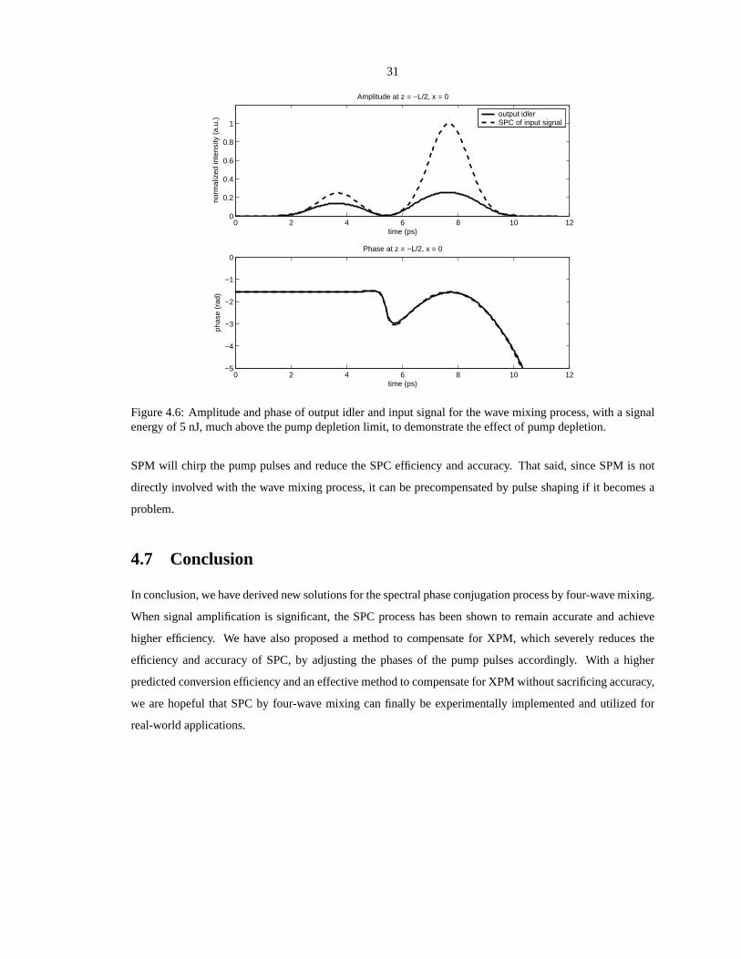
31
0 2 4 6 8 10 120
0.2
0.4
0.6
0.8
1
time (ps)
norm
aliz
ed in
tens
ity (
a.u.
)
Amplitude at z = −L/2, x = 0
0 2 4 6 8 10 12−5
−4
−3
−2
−1
0
time (ps)
phas
e (r
ad)
Phase at z = −L/2, x = 0
output idlerSPC of input signal
Figure 4.6: Amplitude and phase of output idler and input signal for the wave mixing process, with a signalenergy of 5 nJ, much above the pump depletion limit, to demonstrate the effect of pump depletion.
SPM will chirp the pump pulses and reduce the SPC efficiency and accuracy. That said, since SPM is not
directly involved with the wave mixing process, it can be precompensated by pulse shaping if it becomes a
problem.
4.7 Conclusion
In conclusion, we have derived new solutions for the spectral phase conjugation process by four-wave mixing.
When signal amplification is significant, the SPC process has been shown to remain accurate and achieve
higher efficiency. We have also proposed a method to compensate for XPM, which severely reduces the
efficiency and accuracy of SPC, by adjusting the phases of thepump pulses accordingly. With a higher
predicted conversion efficiency and an effective method to compensate for XPM without sacrificing accuracy,
we are hopeful that SPC by four-wave mixing can finally be experimentally implemented and utilized for
real-world applications.
32
Bibliography
[1] D. A. B. Miller, Opt. Lett.5, 300 (1980).
[2] C. Joubert, M. L. Roblin, R. Grousson, Appl. Opt.28, 4604 (1989).
[3] M. Tsang, D. Psaltis, Opt. Lett.28, 1558 (2003).
[4] N. W. Carlson, L. J. Rothberg, A. G. Yodh, W. R. Babbitt, T.W. Mossberg, Opt. Lett.8, 483 (1983).
[5] V. L. da Silva, Y. Silberberg, J. P. Heritage, E. W. Chase,M. A. Saifi, M. J. Andrejco, Opt. Lett.16, 1340
(1991).
[6] A. Rebane, J. Aaviksoo, J. Kuhl, Appl. Phys. Lett.54, 93 (1989).
[7] S. Fraigne, J. P. Galaup, J. L. Le Gouet, B. Bousquet, L. Canioni, M. Joffre, J. P. Likforman, J. Opt. Soc.
Am. B 20, 1555 (2003).
[8] A. M. Weiner, D. E. Leaird, D. H. Reitze, Eung Gi Paek, IEEEJ. Quantum Electron.28, 2251 (1992).
[9] D. Marom, D. Panasenko, R. Rokitski, P. Sun, Y. Fainman, Opt. Lett.25, 132 (2000).
[10] S. Wen, S. Chi, T. Chang, Opt. Lett.19, 939 (1994).
[11] R. Quintero-Torres, M. Thakur, J. Appl. Phys.85, 401 (1999).
[12] A. M. Weiner, Rev. Sci. Instrum.71, 1929 (2000).

33
Chapter 5
Spectral phase conjugation byquasi-phase-matched three-wave mixing
5.1 Introduction
Conventional phase conjugation schemes perform the so-called phase conjugation with spectral inversion [1].
The output of such schemes has a spectrum that is phase conjugated and spectrally inverted with respect to
the input. In the time domain, this is equivalent to phase conjugation of the pulse envelope, so the scheme
is also called temporal phase conjugation (TPC) [2]. A distinct kind of phase conjugation, which performs
phase conjugationwithoutspectral inversion, is first suggested by Miller [3]. The output spectrum of such a
phase conjugation scheme is the phase conjugation of the input spectrum, and the scheme is therefore called
spectral phase conjugation (SPC). In the time domain, the output pulse envelope is the phase conjugation and
time reversal of the input pulse envelope.
While TPC can compensate for even-order dispersion [1], self-phase modulation [4], and intrapulse Ra-
man scattering [5], SPC can simultaneously compensate forall chromatic dispersion [6], self-phase modula-
tion, and self-steepening [2], thus making it attractive for ultrafast applications such as optical communica-
tions. The time reversal operation associated with SPC is also useful for signal processing [7].
The physical implementation of SPC is first suggested by Miller using short-pump four-wave mixing
(FWM) [3], and later demonstrated, for example, using photonecho [8, 9], spectral hole burning [10, 11],
temporal holography [6], spectral holography [12], and spectral three-wave mixing (TWM) [13]. The FWM
scheme is especially appealing to real-world applicationsdue to its simple setup, and its efficiency is recently
shown to be significantly higher than previously considered[14]. However, the FWM scheme requires accu-
rate synchronization of two short pump pulses, which may undermine its robustness. A setup that combines
the elegant geometry of Miller’s scheme and the robustness of TWM can therefore be advantageous. It is also
of fundamental interest to investigate if the use of second-order nonlinearity can provide a higher efficiency
than the FWM configuration.
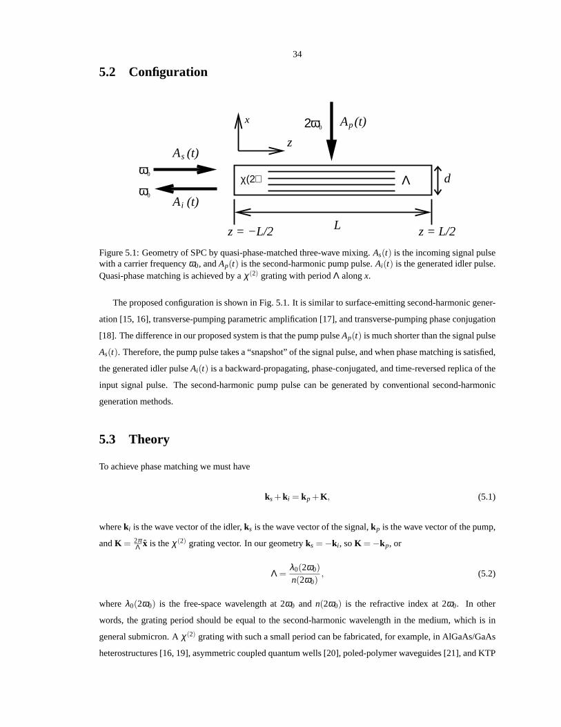
34
5.2 Configuration
A (t)i
A (t)s
2ω0
ω0
ω0
pA (t)x
z
Lz = −L/2 z = L/2
Λ dχ(2)
Figure 5.1: Geometry of SPC by quasi-phase-matched three-wave mixing.As(t) is the incoming signal pulsewith a carrier frequencyω0, andAp(t) is the second-harmonic pump pulse.Ai(t) is the generated idler pulse.Quasi-phase matching is achieved by aχ(2) grating with periodΛ alongx.
The proposed configuration is shown in Fig. 5.1. It is similarto surface-emitting second-harmonic gener-
ation [15, 16], transverse-pumping parametric amplification [17], and transverse-pumping phase conjugation
[18]. The difference in our proposed system is that the pump pulseAp(t) is much shorter than the signal pulse
As(t). Therefore, the pump pulse takes a “snapshot” of the signal pulse, and when phase matching is satisfied,
the generated idler pulseAi(t) is a backward-propagating, phase-conjugated, and time-reversed replica of the
input signal pulse. The second-harmonic pump pulse can be generated by conventional second-harmonic
generation methods.
5.3 Theory
To achieve phase matching we must have
ks+k i = kp +K , (5.1)
wherek i is the wave vector of the idler,ks is the wave vector of the signal,kp is the wave vector of the pump,
andK = 2πΛ x is theχ(2) grating vector. In our geometryks = −k i , soK = −kp, or
Λ =λ0(2ω0)
n(2ω0), (5.2)
whereλ0(2ω0) is the free-space wavelength at 2ω0 and n(2ω0) is the refractive index at 2ω0. In other
words, the grating period should be equal to the second-harmonic wavelength in the medium, which is in
general submicron. Aχ(2) grating with such a small period can be fabricated, for example, in AlGaAs/GaAs
heterostructures [16, 19], asymmetric coupled quantum wells [20], poled-polymer waveguides [21], and KTP
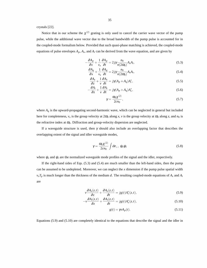
35
crystals [22].
Notice that in our scheme theχ(2) grating is only used to cancel the carrier wave vector of the pump
pulse, while the additional wave vector due to the broad bandwidth of the pump pulse is accounted for in
the coupled-mode formalism below. Provided that such quasi-phase matching is achieved, the coupled-mode
equations of pulse envelopesAp, As, andAi can be derived from the wave equation, and are given by
−∂Ap
∂x+
1vx
∂Ap
∂ t= 2 jγ
n0
n(2ω0)AsAi , (5.3)
∂Aq
∂x+
1vx
∂Aq
∂ t= 2 jγ
n0
n(2ω0)AsAi , (5.4)
∂As
∂z+
1v
∂As
∂ t= jγ(Ap +Aq)A
∗i , (5.5)
−∂Ai
∂z+
1v
∂Ai
∂ t= jγ(Ap +Aq)A
∗s, (5.6)
γ =ω0χ(2)
2cn0, (5.7)
whereAq is the upward-propagating second-harmonic wave, which canbe neglected in general but included
here for completeness,vx is the group velocity at 2ω0 alongx, v is the group velocity atω0 alongz, andn0 is
the refractive index atω0. Diffraction and group-velocity dispersion are neglected.
If a waveguide structure is used, thenγ should also include an overlapping factor that describes the
overlapping extent of the signal and idler waveguide modes,
γ =ω0χ(2)
2cn0
∫
dr⊥, ψsψi (5.8)
whereψs andψi are the normalized waveguide mode profiles of the signal and the idler, respectively.
If the right-hand sides of Eqs. (5.3) and (5.4) are much smaller than the left-hand sides, then the pump
can be assumed to be undepleted. Moreover, we can neglect thex dimension if the pump pulse spatial width
vxTp is much longer than the thickness of the mediumd. The resulting coupled-mode equations ofAs andAi
are
v∂As(z, t)
∂z+
∂As(z, t)∂ t
= jg(t)A∗i (z, t), (5.9)
−v∂Ai(z, t)
∂z+
∂Ai(z, t)∂ t
= jg(t)A∗s(z, t), (5.10)
g(t) = γvAp(t). (5.11)
Equations (5.9) and (5.10) are completely identical to the equations that describe the signal and the idler in

36
the FWM geometry [14]. The boundary conditions are assumed tobe
As(−L2, t) = F(t +
L2v
), (5.12)
Ai(L2, t) = 0. (5.13)
Assuming thatg(t) = |g(t)|exp( jθ), θ is constant, and the pulse width ofAp is much shorter than that ofAs,
Eqs. (5.9) and (5.10) can be solved using the same method described in Ref. [14]. The solution is then given
by
As(z, t) = F(t − zv)cosh[
∫ t
−∞|g(t ′)|dt′], (5.14)
Ai(z, t) = jF ∗(−t − zv)exp( jθ)sinh[
∫ t
−∞|g(t ′)|dt′]. (5.15)
The idler exiting atz= −L2 is
Ai(−L2, t) = jF ∗(−t +
L2v
)exp( jθ)sinh[∫ ∞
−∞|γvAp(t
′)|dt′]. (5.16)
The conversion efficiency, defined as the input signal energydivided by the output idler energy, is
η ≡∫ ∞−∞ |Ai(−L
2 , t ′)|2dt′∫ ∞−∞ |As(−L
2 , t ′)|2dt′= sinh2[
∫ ∞
−∞|γvAp(t
′)|dt′]. (5.17)
Similar to the FWM configuration, the following conditions should be satisfied for accurate SPC operation:
Lv
>> Ts >> Tp >>dvx
, (5.18)
whereTs is the pulse width of the signal.
5.4 Comparison with the FWM scheme
To compare the efficiency of the TWM scheme with that of the FWM scheme, we first compute the pump
energyEp required to achieve a certain conversion efficiencyη by assuming that the pump pulse is a Gaussian,
Ap(t) = Ap0exp(− t2
2T2p
), (5.19)

37
v = c/n0, and the cross-section area of the pump beam isLd. Ep is then given by
Ep =n0Ld2η0
∫
|Ap(t′)|2dt′ (5.20)
=n5
0Ld√πη0ω2
0 [χ(2)]2Tp[sinh−1(
√η)]2, (5.21)
whereη0 is the free-space impedance. Compare this with the total pump energy required for the FWM
configuration, assuming that the two pump pulses are identical,
E′p =
4n′30 Ld
3η0ω0χ(3)sinh−1(
√η) (5.22)
=n′0Ld
ω0n2sinh−1(
√η), (5.23)
wheren′0 is the refractive index of theχ(3) medium. The TWM scheme is thus more efficient when
[
√π
sinh−1(√η)
](ω0Tp)η0[χ(2)]2
n50
>n2
n′0. (5.24)
For example, forλ0 = 800 nm,Tp = 100 fs, a GaAs/AlGaAs heterostructure withχ(2) ≈ 50 pm/V,n0 ≈ 3,
η = 100%, the left-hand side of Eq. (5.24) is about 10−14 cm2/W, which is close to then2 of CS2, but
much lower than that of conjugated polymers (∼ 10−11 cm2/W [23]). That said,χ(2) of asymmetric coupled
GaAs/AlAs quantum wells can theoretically reach 30 nm/V in the far infrared regime [24], potentially giving
rise to a much lower pump energy requirement. The TWM scheme also eliminates the need of the second
pump pulse and avoids the difficulty in synchronizing two ultrashort pulses in a thin medium.
5.5 Numerical analysis
In order to confirm the validity of the approximations in our theoretical predictions, we perform numerical
simulations of Eqs. (5.9) and (5.10), using GaAs/AlGaAs heterostructure as the nonlinear medium, a Gaus-
sian pump pulse withTp = 100 fs, and pump energyEp = 2.1 µJ. The incoming signal is assumed to be
F(t) = As0
−exp[
− 1+ j2
(t +2Ts
Ts)2]+
12
exp[
− 12(t −2Ts
Ts)2]
, (5.25)
with Ts = 1 ps. The calculated conversion efficiency is 100%, consistent with the theoretical efficiency from
Eq. (5.17). The signal and idler pulse shapes from the numerical analysis are plotted in Fig. 5.2, which
confirms that SPC can indeed be accurately performed by TWM. The required pump energy 2.1µJ is much
higher than that theorized in Ref. [14] for the FWM scheme using polydiacetylene (∼ 10 nJ), but it is still
much lower than the pump energy used in Ref. [13] (∼ 1 mJ).
Using the same parameters, Fig. 5.3 plots the theoretical conversion efficiency calculated from Eq. (5.17)

38
−10 −8 −6 −4 −2 0 2 4 6 8 100
0.2
0.4
0.6
0.8
1
time (ps)
inte
nsity
(a.
u.)
(a) Intensity at z = −L/2
−10 −8 −6 −4 −2 0 2 4 6 8 10−3
−2
−1
0
1
2
3
time (ps)
phas
e (r
adia
n)
(b) Phase at z = −L/2
IdlerSignal
Figure 5.2: Plots of intensity and phase of incoming signal and output idler from numerical analysis. It isclear from the plots that the idler is a phase-conjugated andtime-reversed replica of the signal, confirmingour theoretical derivations. Parameters used areχ(2) = 50 pm/V, n0 = 3, L = 1 mm, d = 5 µm, width iny = d, Ep = 2.1 µJ, pump fluence= Ep
Ld . For such dimensions waveguide confinement of the signal andtheidler is necessary.
and that obtained from numerical analysis against the pump energy. The numerical results agree quite well
with the theoretical prediction, although the former is slightly lower, due to slight deviation from the ideal
conditions stated in Eq. (5.18).
5.6 Competing third-order nonlinearity
With a high pump intensity, competing third-order nonlinearity in the form of cross-phase modulation (XPM)
can be detrimental to the SPC accuracy and efficiency in the same manner as for the FWM scheme [14]. One
way to control XPM is by the same XPM compensation method described in Ref. [14], which uses the wave
mixing process to introduce phase variations to the signal and the idler, so that the Kerr phase modulation
due to the strong pump can be exactly canceled. The theoretical proof is very similar to the FWM case [14],
and the pump phase adjustment is
θ(t) = θ0 +∫ t
−∞
3ω0vχ(3)
2cn0|Ap(t
′)|2dt′. (5.26)
This phase adjustment is an almost linear function of time, or equivalently a center frequency shift. Therefore,
if this compensation method is used, theχ(2) grating period should also be adjusted to account for the wave
39
0.5 1 1.5 2 2.5 30
0.2
0.4
0.6
0.8
1
1.2
1.4
1.6
1.8Conversion efficiency comparison
Pump energy (µ J)
Con
vers
ion
effic
ienc
y
theoretical (sinh)simulated
Figure 5.3: Theoretical conversion efficiency derived fromEq. (5.17) and that from numerical analysis plottedagainst pump energy. See caption of Fig. 5.2 for parameters used.
vector change due to the center frequency shift.
5.7 Conclusion
We have proposed a novel SPC scheme by the use of quasi-phase-matched TWM. The advantages of the
TWM scheme over the FWM scheme include the elimination of the second pump pulse, higher conversion
efficiency for certain parameters, and possible independent management of second-order and third-order
nonlinearities.

40
Bibliography
[1] A. Yariv, D. Fekete, and D. M. Pepper, Opt. Lett.4, 52 (1979).
[2] M. Tsang, D. Psaltis, Opt. Lett.28, 1558 (2003).
[3] D. A. B. Miller, Opt. Lett.5, 300 (1980).
[4] R. A. Fisher, B. R. Suydam, and D. Yevick, Opt. Lett.8, 611 (1983).
[5] S. Chi, S. F. Wen, Opt. Lett.19, 1705 (1994).
[6] C. Joubert, M. L. Roblin, and R. Grousson, Appl. Opt.28, 4604 (1989).
[7] D. M. Marom, D. Panasenko, P. Sun, Y. T. Mazurenko, and Y. Fainman, IEEE J. Sel. Top. Quantum
Electron.7, 683 (2001).
[8] N. W. Carlson, L. J. Rothberg, A. G. Yodh, W. R. Babbitt, and T. W. Mossberg, Opt. Lett.8, 483 (1983).
[9] V. L. da Silva, Y. Silberberg, J. P. Heritage, E. W. Chase,M. A. Saifi, and M. J. Andrejco, Opt. Lett.16,
1340 (1991).
[10] A. Rebane, J. Aaviksoo, and J. Kuhl, Appl. Phys. Lett.54, 93 (1989).
[11] S. Fraigne, J. P. Galaup, J. L. Le Gouet, B. Bousquet, L. Canioni, M. Joffre, and J. P. Likforman, J. Opt.
Soc. Am. B20, 1555 (2003).
[12] A. M. Weiner, D. E. Leaird, D. H. Reitze, and Eung Gi Paek,IEEE J. Quantum Electron.28, 2251
(1992).
[13] D. Marom, D. Panasenko, R. Rokitski, P. Sun, and Y. Fainman, Opt. Lett.25, 132 (2000).
[14] M. Tsang and D. Psaltis, Opt. Express12, 2207 (2004).
[15] R. Normandin and G. I. Stegeman, Opt. Lett.4, 58 (1979).
[16] D. Vakhshoori, R. J. Fischer, M. Hong, D. L. Sivco, G. J. Zydzik, G. N. S. Chu, and A. Y. Cho, Appl.
Phys. Lett.59, 896 (1991).
[17] Y. J. Ding, S. J. Lee, and J. B. Khurgin, Phys. Rev. Lett.75, 429 (1995).
41
[18] Y. J. Ding, J. B. Khurgin, and S. J. Lee, Opt. Quantum Electron.28, 1617 (1996).
[19] C. Degen, G. Jennemann, I. Fischer, W. Elsaber, S. Leu, R. Rettig, and W. Stolz, Opt. Quantum Electron.
34, 707 (2002).
[20] S. Janz, F. Chatenoud, and R. Normandin, Opt. Lett.19, 622 (1994).
[21] A. Otomo, G. I. Stegeman, M. C. Flipse, M. B. J. Diemeer, W. H. G. Horsthuis, and G. R. Mohlmann,
J. Opt. Soc. Am. B15, 759 (1998).
[22] C. Canalias, V. Pasiskevicius, R. Clemens, and F. Laurell, Appl. Phys. Lett.82, 4233 (2003).
[23] R. Quintero-Torres and M. Thakur, J. Appl. Phys.85, 401 (1999).
[24] S. Li and J. Khurgin, Appl. Phys. Lett.62, 1727 (1993).

42
Chapter 6
Spontaneous spectral phase conjugationfor coincident frequency entanglement
6.1 Introduction
It has been proven in the two previous chapters that if the three-wave mixing (TWM) or four-wave mixing
(FWM) parametric process is transversely pumped with short pulses in a long and thin nonlinear medium,
parametric amplification can be performed, with time reversal and spectral phase conjugation (SPC) [1, 2].
The correspondence between classical parametric amplification and quantum entanglement makes one won-
der if spontaneous SPC can perform the opposite of what its continuous-wave-pumped counterpart does, and
realize time anticorrelation or frequency correlation. This distinct kind of entanglement is useful for appli-
cations such as quantum-enhanced position and clock synchronization [3] and one-way autocompensating
quantum cryptography [4]. Various implementations of suchentanglement have been suggested [5, 6], and
the scheme proposed by Waltonet al. [6] looks intriguingly similar to the TWM scheme for SPC [1]. On
the other hand, while TWM is traditionally the preferred method to generate entangled photons, recent ex-
perimental progress on entangled photon sources using third-order nonlinear processes [7, 8] makes FWM
a promising candidate for such a task. In this chapter, we prove that spontaneous SPC, either by TWM or
FWM, can indeed efficiently generate time-anticorrelated and frequency-correlated photon pairs.
Our proposed schemes have several key improvements over that in Ref. [6], and make coincident fre-
quency entanglement much more realizable. First, it is unclear in Ref. [6] how phase matching should be
achieved. We propose the incorporation of quasi-phase matching to satisfy the requirement. Second, we
suggest an alternative FWM scheme, which can be more efficientwith focused femtosecond pump beams.
Third, for good efficiency, cross-phase modulation due to the strong pump becomes a large parasitic effect
for both schemes. We introduce the use of pump phase modulation to compensate for cross-phase modula-
tion. We also perform an in-depth Heisenberg analysis of thespontaneous SPC schemes, predicting that a
high gain is possible with current technology. The high gainenables the generation of large-photon-number
frequency-correlated states, which are interesting for their use in nonlocal dispersion cancellation and noise

43
reduction experiments [9].
Lastly we investigate the use of frequency-correlated photons generated by our proposed schemes in the
Hong-Ou-Mandel (HOM) interferometer [10], subject to temporal delays, dispersion, frequency shifts, and
temporal phase modulation. Quantum dispersion cancellation in the HOM interferometer with such photons
has been studied [10, 11, 12, 13], but relatively little attention is given to the distinguishability introduced by
phase modulation in the time domain, for example, via the optical Kerr effect, which can be useful in quantum
nondemolition measurements [14]. Ref. [11] studies the effect of frequency shifts on frequency-correlated
photons, but only in a highly idealized case. Using the formalism developed for our schemes, we first review
the HOM dip effect introduced by time delays and dispersion for completeness, and then study the nonlocal
temporal phase cancellation properties of the entangled photons.
6.2 Configurations
2ω0 pA (t)
A (t)i A (t)s
ω0 ω0
x
z
Lz = −L/2 z = L/2
Λ dχ(2)
Figure 6.1: Spontaneous SPC by TWM.
pA (t)
qA (t)
A (t)sA (t)i
x
z
Lz = −L/2 z = L/2
dχ(3)
Figure 6.2: Spontaneous SPC by FWM.
The spontaneous SPC scheme by TWM is sketched in Fig. 6.1, and the FWM scheme in Fig. 6.2. For the

44
TWM scheme, the interaction Hamiltonian is
H ∝ w∫
dx∫
dzχ(2) f (z)E(+)p E(−)
s E(−)i +H.c., (6.1)
wherew is the width of the nonlinear medium in they dimension,χ(2) is the second-order nonlinear sus-
ceptibility, f (z) is the pump beam profile,E(+) andE(−) are the positive-frequency and negative-frequency
electric field operators, respectively, and the subscriptsp, s, i denote pump, signal and idler, respectively.
If the pump is assumed to be classical, the electric field operators can be written in terms of envelopes,
E(+)p ∝ Ap(t + x
vx)exp(−i2ω0t− ikxx), E(−)
s ∝ A†s(t− z
v)exp(iω0t− ikzz) andE(−)i ∝ A†
i (t +zv)exp(iω0t + ikzz),
wherekx is the pump carrier wave vector, andv andvx are the group velocities inzandx, respectively. Unlike
the scheme in Ref. [5], spontaneous SPC places no restriction on the material dispersion properties as long as
the signal and idler are the same but counterpropagating modes. Otherwise the pump beam(s) can be slightly
tilted in thez direction to compensate fo the signal-idler phase mismatch. The interaction Hamiltonian then
becomes
H ∝ w∫ d
2
− d2
dx∫
dzχ(2) f (z)Ap(t +xvx
)A†s(t −
zv)A†
i (t +zv)exp
[
− i(kx−2πΛ
)x]
+H.c., (6.2)
whereΛ is theχ(2) grating period. Ref. [15] assumes that the transverse dimensiond is small enough so that
detuning due tokx can be ignored. However, for a realizable setup,kx is usually on the order of 1/(1µm),
while d is on the order of microns for a waveguide. Hence in most caseskx should not be ignored, and quasi-
phase matching, not mentioned in Ref. [6], is in fact needed.The submicronχ(2) grating period required can
be fabricated, for example, in a GaAs/AlGaAs heterostructure [16]. To avoid space-time coupling, the spatial
pulse width of the pump, on the order of 100µm for a femtosecond pulse, should be much larger thand ∼10 µm, so that thex dependence ofAp can be neglected.H is then given by
H ∝ wd∫
dzχ(2) f (z)Ap(t)A†s(t −
zv)A†
i (t +zv)+H.c. (6.3)
The FWM process, on the other hand, is automatically phase-matched due to the counterpropagating
pump pulses. The interaction Hamiltonian is
H ∝ w∫
dx∫
dzχ(3) f (z)E(+)p E(+)
q E(−)s E(−)
i +H.c. (6.4)
With similar assumptions as the TWM scheme, the interaction Hamiltonian is given by
H ∝ wd∫
dzχ(3) f (z)Ap(t)Aq(t)A†s(t −
zv)A†
i (t +zv)+H.c., (6.5)
which is almost identical to that of the TWM scheme. Hence one can analyze both schemes in a unified
45
framework, with the general Hamiltonian
H ∝∫
dz f(z)g(t)A†s(t −
zv)A†
i (t +zv)+H.c., (6.6)
whereg(t) ∝ χ(2)Ap(t) for the TWM scheme andg(t) ∝ χ(3)Ap(t)Aq(t) for the FWM scheme. To the first
order, the wave function is given by [6]
|ψ ′〉 ∝∫
dtH|0〉 (6.7)
∝∫
dt∫
dzg(t) f (z)A†s(t −
zv)A†
i (t +zv)|0〉 (6.8)
∝∫
dωs
∫
dωi f (ωs−ωi
v)g(ωs+ωi)a
†s(ωs)a
†i (ωi)|0〉, (6.9)
where f , g, anda†s,i are Fourier transforms off , g, andA†
s,i , respectively. In the time domain, if the width of
g(t) is much more narrow than the width off (z) divided byv, g(t) can sample the integrand in Eq. (6.8), say
at t = 0. Equivalently in the frequency domainf can sample the integrand atωs = ωi in Eq. (6.9). The wave
function becomes
|ψ ′〉 ∝∫
dt′g(t ′)∫
dt f(vt)A†s(−t)A†
i (t)|0〉 (6.10)
∝∫
dω ′ f (ω ′
v)∫
dωg(2ω)a†s(ω)a†
i (ω)|0〉. (6.11)
The generated photon pair therefore possesses quantum timeanticorrelation and frequency correlation. In
summary, for optimal entanglement, the assumption
Lv
>> width of g(t) >>dvx
(6.12)
should be satisfied.
6.3 Conversion efficiency
The efficiency of spontaneous SPC is best studied in the Heisenberg picture. The coupled-operator equations,
assuming classical undepleted pumps, are given by
(
v∂∂z
+∂∂ t
)
As = ig(t)A†i + ic(t)As, (6.13)
(
−v∂∂z
+∂∂ t
)
A†i = −ig∗(t)As− ic(t)A†
i , (6.14)

46
where
g(t) =ω0vχ(2)
2cn0Ap(t) (6.15)
for the TWM scheme and
g(t) =3ω0vχ(3)
4cn0Ap(t)Aq(t) (6.16)
for the FWM scheme.
c(t) =3ω0vχ(3)
4cn0(|Ap|2 + |Aq|2) (6.17)
is the cross-phase modulation term, which acts as a time-dependent detuning factor. Cross-phase modulation
is always present in the FWM scheme, while it exists in the formof competing third-order nonlinearity in the
TWM scheme. Eqs. (6.13) and (6.14) can be solved in the same manner as the classical SPC analysis [1, 2].
The temporary detuning due to cross-phase modulation can becompensated ifg(t) is also appropriately
detuned. Quantitatively, the phase ofg(t) should be modulated as [2],
θ(t) = θ0 +2∫ t
−∞dt′c(t ′). (6.18)
θ(t) can be approximated by a linear temporal phase, or a center frequency shift ofg(t) [2]. In other words,
for spontaneous SPC under the cross-phase modulation effect, the generation of photon pairs will actually be
most efficient at a center frequency different from the center pump frequency in the FWM scheme, or from
half the center second-harmonic pump frequency in the TWM scheme. This is analogous to the phenomenon
of sideband gain in continous-wave FWM, although now the signal and idler spectra shouldcoincidewith
each other. This feature is actually desirable for the FWM scheme, since it is easier to separate the scattered
pump from the weak signal and idler by spectral filtering.
The average number of photons in each mode is
ns = C2ns0 +S2(ni0 +1), (6.19)
ni = C2ni0 +S2(ns0 +1), (6.20)
whereC ≡ cosh[∫
dt|g(t)|], S≡ sinh[∫
dt|g(t)|], ns0 is the initial signal photon number, andni0 is the initial
idler photon number. The number of photon pairs spontaneously generated in each wave mixing event is
thereforeS2, and the conversion efficiency, defined as the energy of the generated photons divided by the

47
energy of the pump photons, is
Γ =2S2hω0
Ep, (6.21)
whereEp is the total pump energy. The FWM scheme is more efficient than the TWM scheme wheng(t) of
the former is larger, or, all else being equal,
χ(3)
(n(3)0 )3
(Ep
ε0cLwTp)
12 &
χ(2)
(n(2)0 )
52
, (6.22)
whereTp is the pump pulse width.
For example, polydiacetylene, a conjugate polymer, has aχ(3) ∼ 10−18 m2/V2 andn(3)0 ∼ 2, while a
GaAs/AlGaAs heterostructure has aχ(2) ∼ 1010 m/V andn(2)0 ∼ 4. For a focused femtosecond pump beam,
sayL ∼ 2 mm,w∼ 5 µm, Tp ∼ 100 fs, the FWM scheme is more efficient whenEp is approximately larger
than 1 nJ. Ti:Sapphire laser systems can achieve a pulse energy of 1 mJ or more, so the FWM scheme can be
orders of magnitude more efficient. The FWM scheme also has theadvantage of automatic phase matching
as well as having pump pulses near the fundamental frequency, thus eliminating the need of quasi-phase
matching and a second-harmonic source in an experiment. That said, the necessity of synchronizing two
short pump pulses in the FWM scheme may undermine its robustness, while the TWM scheme may be more
efficient for certain parameters and it is relatively easierto filter out scattered second-harmonic pump from
the signal and idler. For the parameters above, the signal and idler gainS2 can achieve 100% for a pump pulse
energy∼ 10 nJ with the FWM scheme and∼ 2 µJ with the TWM scheme. For such a relatively high gain
the wave function can have higher-order terms [17],|ψ〉 ∝ ∑∞n=0Tn|n〉s|n〉i , whereT = S/C, and the weights
of large-photon-number statesT2n with n > 1 become appreciable whenS2 approaches unity. Amplification
of coincident frequency entanglement [17] also becomes possible.
6.4 Hong-Ou-Mandel interferometry
In the HOM interferometry, variable delays are introduced to the signal and idler photons, which then pass
through a 50-50 beam splitter and finally the coincidence rate of the two output ports is measured [10]. For
simplicity we also assume that the distances from the two detectors to the beam splitter are the same. We start
with the more general wave function in Eq. (6.8). The electric field operators of the two outputs are given by
A1,2(t) ∝ As,i(±Ls,i , t)+ iAi,s(∓Li,s, t), (6.23)

48
whereLs,i are the distances travelled by the signal and the idler fromz= 0 to the detectors, respectively.Li
has a negative sign in front because the idler travels backwards. The coincidence rate is given by [12, 13]
Pc ∝∫
dt1
∫
dt2〈ψ ′|A†1(t1)A
†2(t2)A1(t1)A2(t2)|ψ ′〉 (6.24)
∝∫
dt+|g(t+ − L+
v)|2[
∫
dt−| f (L−−vt−)|2−Re∫
dt− f ∗(L−−vt−) f (L− +vt−)]
. (6.25)
wheret+ = (t1 + t2)/2, L+ = (Ls+Li)/2, t− = (t1− t2)/2 andL− = (Ls−Li)/2 is half the signal-idler path
difference. The shape of the HOM dip with respect to the path differenceLs−Li is given by the last term of
Eq. (6.25), which has a width on the order ofL, the width of the pump beam profilef (z). Ref. [11] predicts
that Pc is identically zero for allL− with perfectly frequency-correlated photons, which is simply a special
case whenL → ∞.
Steinberget al. predicted [18] and demonstrated [19] even-order dispersion cancellation in the HOM
interferometer with frequency-anticorrelated photons. With frequency-correlated photons, intuition then sug-
gests that one can obtain nonlocal cancellation of dispersion of all orders, which is proven in Ref. [12]. To see
how this effect manifests itself in our schemes, we shall start with the general wave function in the frequency
domain, Eq. (6.9), and apply spectral phase to the operatorsjust as in Ref. [18]. The coincidence rate can be
expressed in terms of frequency-domain operators as [18]
Pc ∝∫
dω1
∫
dω2〈ψ ′|a†1(ω1)a
†2(ω2)a1(ω1)a2(ω2)|ψ ′〉 (6.26)
∝∫
dω1
∫
dω2|g(ω1 +ω2)|2
| f (ω1−ω2
v)|2−
Re[
f (ω1−ω2
v) f ∗(
ω2−ω1
v)exp
(
i[ks(ω1)−ks(ω2)]Ls− i[ki(ω1)−ki(ω2)]Li
)]
. (6.27)
whereks andki are the dispersive propagation constants of the signal and idler, respectively. The exponential
term in Eq. (6.27) characterizes the nonlocal dispersion cancellation. If the photons have perfect frequency
anticorrelation, ˜g is infinitely sharp,ω1 =−ω2, and we recover the even-order dispersion cancellation results
in Ref. [18]. If f is infinitely sharp,ω1 = ω2, the exponential term evalulates to 1 andPc = 0 for dispersion
of all orders. If f is not infinitely sharp and dispersion is only due to time delay, the result in Eq. (6.25) is
recovered.
Frequency shifts can be introduced to the signal and the idler by, for example, moving mirrors or acousto-
optic modulators via the Doppler effect. Opposite Doppler shifts can also occur to the counterpropagating
photons if the source frame is moving alongz relative to the detection frame. We can then rewriteA1 andA2,
A1,2(t) ∝ exp(−iδωs,it)As,i + i exp(−iδωi,st)Ai,s, (6.28)
whereδωs is the signal frequency shift andδωi is the idler frequency shift. For intuitiveness we assume that
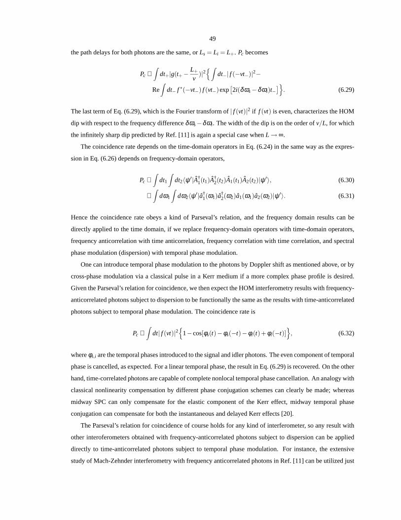
49
the path delays for both photons are the same, orLs = Li = L+. Pc becomes
Pc ∝∫
dt+|g(t+ − L+
v)|2
∫
dt−| f (−vt−)|2−
Re∫
dt− f ∗(−vt−) f (vt−)exp[
2i(δωs−δωi)t−]
. (6.29)
The last term of Eq. (6.29), which is the Fourier transform of| f (vt)|2 if f (vt) is even, characterizes the HOM
dip with respect to the frequency differenceδωs−δωi . The width of the dip is on the order ofv/L, for which
the infinitely sharp dip predicted by Ref. [11] is again a special case whenL → ∞.
The coincidence rate depends on the time-domain operators in Eq. (6.24) in the same way as the expres-
sion in Eq. (6.26) depends on frequency-domain operators,
Pc ∝∫
dt1
∫
dt2〈ψ ′|A†1(t1)A
†2(t2)A1(t1)A2(t2)|ψ ′〉, (6.30)
∝∫
dω1
∫
dω2〈ψ ′|a†1(ω1)a
†2(ω2)a1(ω1)a2(ω2)|ψ ′〉. (6.31)
Hence the coincidence rate obeys a kind of Parseval’s relation, and the frequency domain results can be
directly applied to the time domain, if we replace frequency-domain operators with time-domain operators,
frequency anticorrelation with time anticorrelation, frequency correlation with time correlation, and spectral
phase modulation (dispersion) with temporal phase modulation.
One can introduce temporal phase modulation to the photons by Doppler shift as mentioned above, or by
cross-phase modulation via a classical pulse in a Kerr medium if a more complex phase profile is desired.
Given the Parseval’s relation for coincidence, we then expect the HOM interferometry results with frequency-
anticorrelated photons subject to dispersion to be functionally the same as the results with time-anticorrelated
photons subject to temporal phase modulation. The coincidence rate is
Pc ∝∫
dt| f (vt)|2
1−cos[φs(t)−φs(−t)−φi(t)+φi(−t)]
, (6.32)
whereφs,i are the temporal phases introduced to the signal and idler photons. The even component of temporal
phase is cancelled, as expected. For a linear temporal phase, the result in Eq. (6.29) is recovered. On the other
hand, time-correlated photons are capable of complete nonlocal temporal phase cancellation. An analogy with
classical nonlinearity compensation by different phase conjugation schemes can clearly be made; whereas
midway SPC can only compensate for the elastic component of the Kerr effect, midway temporal phase
conjugation can compensate for both the instantaneous and delayed Kerr effects [20].
The Parseval’s relation for coincidence of course holds forany kind of interferometer, so any result with
other interoferometers obtained with frequency-anticorrelated photons subject to dispersion can be applied
directly to time-anticorrelated photons subject to temporal phase modulation. For instance, the extensive
study of Mach-Zehnder interferometry with frequency anticorrelated photons in Ref. [11] can be utilized just

50
as well in the time domain.
6.5 Conclusion
In conclusion, spontaneous SPC schemes by TWM and FWM are studied and compared under a general
framework. It is proven that spontaneous SPC is capable of generating entangled photon pairs with time
anticorrelation and frequency correlation. The use of quasi-phase matching and four-wave mixing is also
proposed to improve the efficiency. Just as in the classical analysis, pump phase modulation is shown to
effectively compensate for detuning due to cross-phase modulation.

51
Bibliography
[1] M. Tsang and D. Psaltis, Opt. Commun.242, 659 (2004).
[2] M. Tsang and D. Psaltis, Opt. Express12, 2207 (2004).
[3] V. Giovannetti, S. Lloyd, and L. Maccone, Nature (London) 412, 417 (2001).
[4] Z. D. Walton, A. F. Abouraddy, A. V. Sergienko, B. E. A. Saleh, and M. C. Teich, Phys. Rev. A67,
062309 (2003).
[5] V. Giovannetti, L. Maccone, J. H. Shapiro, and F. N. C. Wong, Phys. Rev. Lett.88, 183602 (2002).
[6] Z. D. Walton, M. C. Booth, A. V. Sergienko, B. E. A. Saleh, and M. C. Teich, Phys. Rev. A67, 053810
(2003).
[7] M. Fiorentino, P. L. Voss, J. E. Sharping, and P. Kumar, IEEE Photon. Technol. Lett.14, 983 (2002).
[8] X. Li, J. Chen, P. Voss, J. Sharping, and P. Kumar, Opt. Express12, 3737 (2004).
[9] M. J. Fitch and J. D. Franson, Phys. Rev. A65, 053809 (2002).
[10] C. K. Hong, Z. Y. Ou, and L. Mandel, Phys. Rev. Lett.59, 2044 (1987).
[11] R. A. Campos, B. E. A. Saleh, and M. C. Teich, Phys. Rev. A42, 4127 (1990).
[12] R. Erdmann, D. Branning, W. Grice, and I. A. Walmsley, Phys. Rev. A62, 053810 (2000).
[13] V. Giovannetti, L. Maccone, J. H. Shapiro, and F. N. C. Wong, Phys. Rev. A66, 043813 (2002).
[14] N. Imoto, H. A. Haus, and Y. Yamamoto, Phys. Rev. A32, 2287 (1985).
[15] A. De Rossi and V. Berger, Phys. Rev. Lett.88, 043901 (2002).
[16] D. Vakhshoori, R. J. Fischer, M. Hong, D. L. Sivco, G. J. Zydzik, G. N. S. Chu, and A. Y. Cho, Appl.
Phys. Lett.59, 896 (1991).
[17] F. De Martini, Phys. Rev. Lett.81, 2842 (1998).
[18] A. M. Steinberg, P. G. Kwiat, and R. Y. Chiao, Phys. Rev. A45, 6659 (1992).

52
[19] A. M. Steinberg, P. G. Kwiat, and R. Y. Chiao, Phys. Rev. Lett.68, 2421 (1992).
[20] M. Tsang and D. Psaltis, Opt. Lett.28, 1558 (2003).

53
Chapter 7
Spectral phase conjugation via extendedphase matching
7.1 Introduction
In contrast with the more conventional optical phase conjugation schemes that perform phase conjugation
with spectral inversion [1], spectral phase conjugation (SPC) is the phase conjugation of an optical signal
in the frequency domain without spectral inversion. Equivalently, in the time domain, SPC is the phase
conjugation and time reversal of the signal complex pulse envelope [2]. SPC is useful for all-order dispersion
and nonlinearity compensation [3, 4], as well as optical signal processing [5]. Although SPC has been
experimentally demonstrated using photon echo [6, 7], spectral hole burning [8, 9], temporal holography [3],
spectral holography [10], and spectral three-wave mixing (TWM) [11], all the demonstrated schemes suffer
from the use of cryogenic setups, nonrealtime operation, orextremely high pump energy. Pulsed TWM [12]
and four-wave-mixing (FWM) [2, 13] processes in the transverse-pumping geometry have been theoretically
proposed to efficiently perform SPC, but have not yet been experimentally realized. All the holographic and
wave-mixing schemes also have strict requirements on the transverse beam profile of the signal, limiting their
appeal for simultaneous diffraction and dispersion compensation applications.
There is a correspondence between classical SPC and quantumcoincident frequency entanglement, as
shown in Ref. [14] for the transversely pumped TWM [15, 12] andFWM [2, 13] processes. It is then
interesting to see if other coincident frequency entanglement schemes are also capable of performing SPC,
when an input signal is present. This chapter studies one of such schemes, which makes use of extended
phase matching (EPM)[16] and has been experimentally demonstrated [17] in a periodically-poled potassium
titanyl phosphate (PPKTP) crystal [18]. It is shown in Section 7.3, for the first time to the author’s knowledge,
that this EPM scheme is indeed capable of performing SPC and optical parametric amplification (OPA), more
efficiently than previous proposals.
The analysis also yields a surprising result, namely that the parametric gain can be theoretically infinite
even for a pump pulse with finite energy, analogous to backward wave oscillation, where counterpropagating
54
waves are parametrically coupled and can give rise to mirrorless optical parametric oscillation (OPO)[19,
20, 21, 22, 23, 24, 25]. The reason for the similarity is that,in the scheme presented here, even though the
signal and the idler copropagate with the pump pulse in the laboratory frame, theycounterpropagate in the
frame of the moving pump pulse, because one is faster than the pump and one is slower. Hence the moving
pump pulse provides both an effective cavity and parametricgain, leading to oscillation. In reality, however,
the interaction among the pulses should be ultimately limited by the finite device length. It is shown in
Section 7.4, with a Laplace analysis, that the parametric gain should abruptly increase above the threshold,
where infinite gain is predicted by the Fourier analysis, buta finite medium length will always limit the
gain to a finite value. Still, as previous proposals of TWM mirrorless OPO have never been experimentally
achieved due to the requirement of a continuous-wave (CW) pump and the difficulty in phase matching
counterpropagating waves, the presented analysis suggests the exciting possibility that mirrorless OPO can
be realized with an ultrashort pump pulse and a practical poling period for phase matching of copropagating
modes, if a long enough medium can be fabricated and parasitic effects can be controlled. By analyzing the
scheme in the Heisenberg picture in Section 7.5, a high spontaneous parametric down conversion rate is also
predicted, in excellent agreement with the experimental result reported in Ref. [17]. The result should be
useful for many quantum information processing applications, such as quantum-enhanced synchronization
[26] and multiphoton entanglement for quantum cryptography [27]. Finally, numerical results are presented
in Section 7.6, which confirm the theoretical predictions.
7.2 Setup
Figure 7.1: Schematic of spectral phase conjugation (SPC) via type-II extended phase matching (EPM). Thesignal and idler pulses, in orthogonal polarizations, havecarrier frequencies ofωs andωi , while the pumppulse has a carrier frequency ofωp = ωs + ωi . The EPM condition requires that the signal and the idlercounterpropagate with respect to the pump, which should be much shorter than the input signal.
Consider the copropagating TWM process (Fig. 7.1), assumingthat the basic type-II phase matching
condition (ks + ki = kp + 2π/Λ), with a quasi-phase-matching periodΛ, is satisfied. The coupled-mode

55
equations are
∂Ap
∂z+k′p
∂Ap
∂ t= jχpAsAi , (7.1)
∂As
∂z+k′s
∂As
∂ t= jχsApA∗
i , (7.2)
∂A∗i
∂z+k′i
∂A∗i
∂ t= − jχiA
∗pAs, (7.3)
whereAp is the pump pulse envelope of carrier frequencyωp, As,i are the signal and idler envelopes of
frequenciesωs andωi , respectively,k′p,s,i are the group delays of the three modes,χp,s,i ≡ ωp,s,i χ(2)/(2cnp,s,i)
are the nonlinear coupling coefficients,ωp,s,i are the center frequencies of the modes such thatωs+ωi = ωp,
andnp,s,i are the refractive indices. Group-velocity dispersion within each mode and diffraction are neglected.
Defineτ ≡ t − k′pz as the retarded time coordinate that follows the propagating pump pulse. The change of
coordinates yields
∂Ap
∂z= jχpAsAi , (7.4)
∂As
∂z+(k′s−k′p)
∂As
∂τ= jχsApA∗
i , (7.5)
∂A∗i
∂z+(k′i −k′p)
∂A∗i
∂τ= − jχiA
∗pAs. (7.6)
Throughout the theoretical analysis, the pump is assumed tobe undepleted and unchirped, so thatAp =
Ap0(t −k′pz) = Ap0(τ), hereafter regarded as real without loss of generality.
7.3 Fourier analysis
Equations (7.5) and (7.6) are space-invariant, if the nonlinear medium lengthL is much longer than the signal
or idler spatial pulse width in the frame ofzandτ, or
L >>Ts,i
|k′s,i −k′p|, (7.7)
whereTs,i is the signal or idler pulse width. One can then perform Fourier transform on the equations with
respect toz, as defined by the following,
As(κ,τ) ≡∫ ∞
−∞As(z,τ)exp(− jκz)dz, (7.8)
A∗i (κ,τ) ≡
∫ ∞
−∞A∗
i (z,τ)exp(− jκz)dz. (7.9)
56
Notice thatA∗i is defined as the Fourier transform after the conjugation ofAi . The coupled-mode equations
become
jκAs+(k′s−k′p)∂ As
∂τ= jχsAp0(τ)A∗
i , (7.10)
jκA∗i +(k′i −k′p)
∂ A∗i
∂τ= − jχiAp0(τ)As. (7.11)
Let
γs ≡ k′s−k′p, γi ≡ k′i −k′p, r ≡∣
∣
∣
γsχi
γi χs
∣
∣
∣. (7.12)
Consider the case in whichγs andγi are nonzero and have opposite signs, implying that the signal and the idler
propagate in opposite directions with respect to the pump. This can be achieved for a range of wavelengths
in KTP. Without loss of generality, assume thatγs > 0 andγi < 0, so thatk′s > k′p > k′i . Making the following
substitutions,
A =√
rAsexp( jκγs
τ), B = A∗i exp( j
κγi
τ), (7.13)
one obtains
∂A∂τ
= j
√
∣
∣
∣
χsχi
γsγi
∣
∣
∣Ap0(τ)Bexp
[
jκ(1γs
− 1γi
)τ]
, (7.14)
∂B∂τ
= j
√
∣
∣
∣
χsχi
γsγi
∣
∣
∣Ap0(τ)Aexp[
− jκ(1γs
− 1γi
)τ]
. (7.15)
Due to linear space invariance, the wave-mixing process cannot generate new spatial frequencies (κ) for A
andB. The magnitude ofκ then depends only on the initial bandwidths ofA andB, and is on the order of
2πγs,i/Ts,i . As a result, if the pump pulse widthTp is much shorter than the minimum period of the detuning
factor exp[± jκ(1/γs−1/γi)τ], or
Tp <<∣
∣
∣
2πκ(1/γs−1/γi)
∣
∣
∣∼∣
∣
∣
Ts,i
γs,i(1/γs−1/γi)
∣
∣
∣, (7.16)
the pump can effectively sample the detuning factor, say, atτ = 0. Defining a normalized coupling function,
g(τ) ≡√
∣
∣
∣
χsχi
γsγi
∣
∣
∣Ap0(τ), (7.17)
57
two simple coupled-mode equations are obtained,
∂A∂τ
= jg(τ)B, (7.18)
∂B∂τ
= jg(τ)A. (7.19)
Because the signal and the idler counterpropagate with respect to the pump, the signal should begin to mix
with the pump at the leading edge of the pump pulse, say atτ = −Tp/2, while the idler should begin to mix
at the trailing edge of the pump, say atτ = Tp/2. The solutions of Eqs. (7.18) and (7.19) can then be written
as
A(κ,τ) = sec(G)
A(κ,−Tp
2)cos
[
∫ τ
Tp/2g(τ ′)dτ ′
]
+ jB(κ,Tp
2)sin
[
∫ τ
−Tp/2g(τ ′)dτ ′
]
, (7.20)
B(κ,τ) = sec(G)
jA(κ,−Tp
2)sin
[
∫ τ
Tp/2g(τ ′)dτ ′
]
+B(κ,Tp
2)cos
[
∫ τ
−Tp/2g(τ ′)dτ ′
]
, (7.21)
where
G≡∫ Tp/2
−Tp/2g(τ)dτ ≈
∫ ∞
−∞g(τ)dτ. (7.22)
The input signal pulse is required to be placed in advance of the pump (byts >> Ts), and the input idler pulse
to be placed behind the pump (delayed byti >> Ti), so that the signal and the idler only overlap the pump
pulse inside the nonlinear medium. Consequently, the output solutions are
As(L, t) = As0(t −k′sL+ ts)sec(G)+ j1√rA∗
i0
(
− 1r(t −k′sL− ti)
)
tan(G), (7.23)
Ai(L, t) = Ai0(t −k′iL− ti)sec(G)+ j√
rA∗s0
(
− r(t −k′iL+ ts))
tan(G). (7.24)
To see how the device is able to perform SPC, assume that the center frequencies of the two modes are the
same,ωs = ωi , χs = χi , and the type-II EPM condition,
k′s+k′i = 2k′p, k′s 6= k′i , (7.25)
which depends on the material dispersion properties and typically occurs at a single set of center frequencies,
is satisfied [16]. Thenr = 1, and the output idler becomes the phase-conjugated and time-reversed replica of
the input signal, if the input idler is zero. SPC is hence performed. The SPC efficiencyη , or the idler gain,
defined as the output idler fluence divided by the input signalfluence, is
η ≡∫ ∞−∞ |Ai(L, t)|2dt∫ ∞−∞ |As(0, t)|2dt
= tan2(G). (7.26)
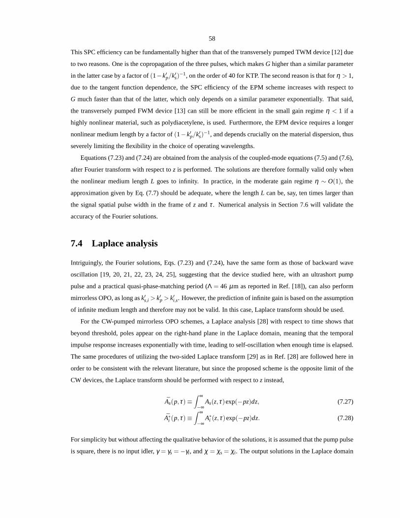
58
This SPC efficiency can be fundamentally higher than that of the transversely pumped TWM device [12] due
to two reasons. One is the copropagation of the three pulses,which makesG higher than a similar parameter
in the latter case by a factor of(1−k′p/k′s)−1, on the order of 40 for KTP. The second reason is that forη > 1,
due to the tangent function dependence, the SPC efficiency ofthe EPM scheme increases with respect to
G much faster than that of the latter, which only depends on a similar parameter exponentially. That said,
the transversely pumped FWM device [13] can still be more efficient in the small gain regimeη < 1 if a
highly nonlinear material, such as polydiacetylene, is used. Furthermore, the EPM device requires a longer
nonlinear medium length by a factor of(1−k′p/k′s)−1, and depends crucially on the material dispersion, thus
severely limiting the flexibility in the choice of operatingwavelengths.
Equations (7.23) and (7.24) are obtained from the analysis of the coupled-mode equations (7.5) and (7.6),
after Fourier transform with respect toz is performed. The solutions are therefore formally valid only when
the nonlinear medium lengthL goes to infinity. In practice, in the moderate gain regimeη ∼ O(1), the
approximation given by Eq. (7.7) should be adequate, where the lengthL can be, say, ten times larger than
the signal spatial pulse width in the frame ofz andτ. Numerical analysis in Section 7.6 will validate the
accuracy of the Fourier solutions.
7.4 Laplace analysis
Intriguingly, the Fourier solutions, Eqs. (7.23) and (7.24), have the same form as those of backward wave
oscillation [19, 20, 21, 22, 23, 24, 25], suggesting that thedevice studied here, with an ultrashort pump
pulse and a practical quasi-phase-matching period (Λ = 46 µm as reported in Ref. [18]), can also perform
mirrorless OPO, as long ask′s,i > k′p > k′i,s. However, the prediction of infinite gain is based on the assumption
of infinite medium length and therefore may not be valid. In this case, Laplace transform should be used.
For the CW-pumped mirrorless OPO schemes, a Laplace analysis [28] with respect to time shows that
beyond threshold, poles appear on the right-hand plane in the Laplace domain, meaning that the temporal
impulse response increases exponentially with time, leading to self-oscillation when enough time is elapsed.
The same procedures of utilizing the two-sided Laplace transform [29] as in Ref. [28] are followed here in
order to be consistent with the relevant literature, but since the proposed scheme is the opposite limit of the
CW devices, the Laplace transform should be performed with respect toz instead,
As(p,τ) ≡∫ ∞
−∞As(z,τ)exp(−pz)dz, (7.27)
A∗i (p,τ) ≡
∫ ∞
−∞A∗
i (z,τ)exp(−pz)dz. (7.28)
For simplicity but without affecting the qualitative behavior of the solutions, it is assumed that the pump pulse
is square, there is no input idler,γ = γs = −γi , andχ = χs = χi . The output solutions in the Laplace domain

59
are then given by
As(p,Tp
2) =
√1−P2csc(G
√1−P2)
P+√
1−P2cot(G√
1−P2)As(p,−Tp
2), (7.29)
A∗i (p,−Tp
2) =
− j
P+√
1−P2cot(G√
1−P2)As(p,−Tp
2), (7.30)
P≡ pχAp0
, G≡ χAp0(Tp
γ). (7.31)
If we let p = jκ , the transfer functions in Eqs. (7.29) and (7.30) are well-known to be low-pass filters [30],
the bandwidth of which decreases asG increases. If the spatial bandwidth of the input signal, on the order
of γ/Ts, is much smaller than the bandwidth of the low-pass filters, the transfer functions can be regarded as
flat-top functions, and by pluggingP = 0 in Eqs. (7.29) and (7.30), the Fourier solutions in Eqs. (7.23) and
(7.24) are recovered. ForG << 1, the transfer functions are sinc functions with a bandwidth ∼ γ/Tp, so the
Fourier solutions are valid ifTp << Ts, which is essentially the same assumption used in the Fourier analysis,
Eq. (7.16). AsG increases and the filter bandwidth decreases, however, the Fourier solutions become less
and less accurate for a finite-bandwidth input signal.
The poles of the transfer functions,p∞, can be obtained by setting the denominator of Eqs. (7.29) and
(7.30) to zero,
p∞ +√
(χAp0)2− p2∞ cot
[
G√
1− p2∞/(χAp0)2
]
= 0. (7.32)
0 1 2 3 4 5 60
0.1
0.2
0.3
0.4
0.5
0.6
0.7
0.8
0.9
1
G
P
Positive Poles of Transfer Functions
Figure 7.2: Normalized polesp∞/(χAp0) plotted againstG, obtained by numerically solving Eq. (32), indi-cating the onset of spatial instability beyond the threshold G > π/2. More poles appear asG is increased.

60
Figure 7.2 plots the normalized polesp∞/(χAp0) againstG. Positive poles begin to appear whenG> π/2,
hence thespatial impulse response increases exponentially with respect toz beyond threshold.
It is interesting to compare the scheme studied here with thecase in which the pump, signal, and idler
have degenerate group delays (k′p = k′s = k′i )[31]. The coupled-mode equations of the latter case are
∂As,i(z,τ)
∂z= jχAp0(τ)A∗
i,s(z,τ), (7.33)
where theτ derivatives vanish. The solutions are easily seen to be
As,i(z,τ) = As,i(0,τ)cosh[χAp0(τ)z]+ jA∗i,s(0,τ)sinh[χAp0(τ)z]. (7.34)
This corresponds to theG→ ∞ limit of the former scheme, wherep∞/(χAp0)→ 1 and all the poles approach
the growth rate of the degenerate case,χAp0.
7.5 Spontaneous parametric down conversion
Given the input-output signal-idler relationship in Eqs. (7.23) and (7.24), it is straightforward to obtain a
quantum picture of the parametric process in the moderate gain regime by replacing the signal and idler
envelopes with Heisenberg operators, so that
As = As0sec(G)+ jA†i0 tan(G), (7.35)
Ai = jA†s0 tan(G)+ Ai0sec(G). (7.36)
If the inputs are Fock states,
ns,i ≡ 〈A†s,iAs,i〉 = 〈As,iA
†s,i〉−1, (7.37)
〈A†s0Ai0〉 = 〈A†
i0As0〉 = 〈As0A†i0〉 = 〈Ai0A†
s0〉 = 0. (7.38)
The average output photon number of each mode is
ns = ns0sec2(G)+(ni0 +1) tan2(G), (7.39)
ni = ni0sec2(G)+(ns0 +1) tan2(G). (7.40)
The average number of spontaneously generated photon pairsper pump pulse is therefore the same as the
idler gain, orη = tan2(G). Moreover, the unitary transform given by Eqs. (7.35) and (7.36) has the same
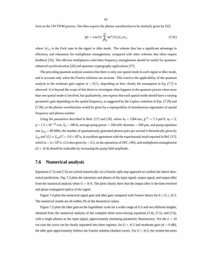
61
form as the CW FWM process. One then expects the photon wavefunction to be similarly given by [32]
|ψ〉 = cos(G)∞
∑n=0
sinn(G)|n〉s|n〉i , (7.41)
where|n〉s,i is the Fock state in the signal or idler mode. The scheme thus has a significant advantage in
efficiency and robustness for multiphoton entanglement, compared with other schemes that often require
feedback [33]. The efficient multiphoton coincident frequency entanglement should be useful for quantum-
enhanced synchronization [26] and quantum cryptography applications [27].
The preceding quantum analysis assumes that there is only one spatial mode in each signal or idler mode,
and is accurate only when the Fourier solutions are accurate. This restricts the applicability of the quantum
analysis to the moderate gain regimeη ∼ O(1), depending on how closely the assumption in Eq. (7.7) is
observed. It is beyond the scope of this thesis to investigate what happens in the quantum picture when more
than one spatial mode is involved, but qualitatively, one expects that each spatial mode should have a varying
parametric gain depending on the spatial frequency, as suggested by the Laplace solutions in Eqs. (7.29) and
(7.30), so the photon wavefunction would be given by a superposition of simultaneous eigenstates of spatial
frequency and photon number.
Using the parameters described in Refs. [17] and [18], whereλ0 = 1584 nm,χ(2) = 7.3 pm/V, n0 = 2,
γ = 1.5×10⁻¹⁰ s/m,Tp = 100 fs, average pump power= 350 mW, diameter= 200µm, and pump repetition
rate frep = 80 MHz, the number of spontaneously generated photon pairs per second is theoretically given by
freptan2(G)≈ frepG2 = 3.6×10⁶/s, in excellent agreement with the experimental result reported in Ref. [17],
which is∼ 4×10⁶/s. G is then given by∼ 0.2, so the operations of SPC, OPA, and multiphoton entanglement
(G > π/4) should be realizable by increasing the pump field amplitude.
7.6 Numerical analysis
Equations (7.5) and (7.6) are solved numerically via a Fourier split-step approach to confirm the above theo-
retical predictions. Fig. 7.3 plots the intensities and phases of the input signal, output signal, and output idler
from the numerical analysis whenG = π/4. The plots clearly show that the output idler is the time-reversed
and phase-conjugated replica of the signal.
Figure 7.4 plots the numerical signal gain and idler gain compared with Fourier theory for 0< G≤ π/3.
The numerical results are all within 3% of the theoretical values.
Figure 7.5 plots the idler gain on the logarithmic scale for awider range ofG’s and two different lengths,
obtained from the numerical analysis of the complete three-wave-mixing equations (7.4), (7.5), and (7.6),
with a single photon as the input signal, approximately emulating parametric fluorescence. For theL = 10
cm case the curve can be clearly separated into three regimes; for G < π/2 and moderate gain (η ∼ 0 dB),
the idler gain approximately follows the Fourier solution (dashed curve). ForG > π/2, the system becomes
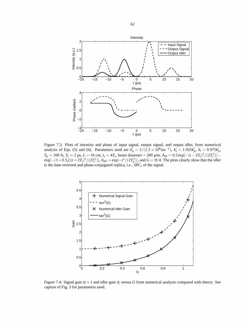
62
−20 −15 −10 −5 0 5 10 15 200
0.5
1
1.5
2Intensity
Inte
nsity
(a.
u.)
τ (ps)
−20 −15 −10 −5 0 5 10 15 20−4
−2
0
2
4Phase
Pha
se (
radi
an)
τ (ps)
Input SignalOutput SignalOutput Idler
Figure 7.3: Plots of intensity and phase of input signal, output signal, and output idler, from numericalanalysis of Eqs. (5) and (6). Parameters used arek′p = 1/(1.5× 108ms−1), k′s = 1.025k′p, ki = 0.975k′p,Tp = 100 fs,Ts = 2 ps,L = 10 cm,ts = 4Ts, beam diameter = 200µm, As0 = 0.5exp[−(t −2Ts)
2/(2T2s )]−
exp[−(1+0.5 j)(t +2Ts)2/(2T2
s )], Ap0 = exp[−t2/(2T2p )], andG= π/4. The plots clearly show that the idler
is the time-reversed and phase-conjugated replica, i.e., SPC, of the signal.
0 0.2 0.4 0.6 0.8 10
0.5
1
1.5
2
2.5
3
3.5
4
4.5
5
G
Gai
n
Numerical Signal Gain
sec2(G)
Numerical Idler Gain
tan2(G)
Figure 7.4: Signal gainη +1 and idler gainη versusG from numerical analysis compared with theory. Seecaption of Fig. 3 for parameters used.
63
0 0.5 1 1.5 2 2.5−50
0
50
100
150
G
dB
10log10
(η) (L = 10 cm)
10log10
(η) (L = 1 cm)
10log10
[tan2(G)]
Figure 7.5: Plot of numerical idler gainη in dB againstG for L = 10 cm (solid) andL = 1 cm (dash-dot),compared with the Fourier theory (dash), tan2(G) in dB. Three distinct regimes can be observed for theL = 10cm case; the moderate gain regime where the Fourier theory isaccurate, the unstable regime where the gainincreases exponentially, and the oscillation regime wheresignificant pump depletion occurs. ForL = 1 cm,the medium is not long enough for oscillation to occur in the parameter range of interest.
unstable and an exponential growth (linear ramp on the logarithmic curve) is observed, until the pump is
significantly depleted, parametric oscillation occurs, and the exponential growth abruptly stops.
ForL = 1 cm, the numerical solution departs from theory for a smaller G, and the slope of the logarithmic
curve in the unstable regime, proportional toL, is too small to initiate oscillation in the parameter rangeof
interest.
A medium length of 10 cm may be pushing the limit of current technology. Even if one is able to fabricate
such a long periodically-poled nonlinear crystal, the effective medium length is always limited by parasitic
effects, such as diffraction, group-velocity dispersion,and competing third-order nonlinearities, so it might
be difficult to fabricate an ideal EPM device for the aforementioned purposes. For instance, in the experiment
by Kuzucuet al. [17], the diameter of the beam isW ∼ 200 µm, so the characteristic diffraction length is
∼W2/λ0 = 4 cm, while the characteristic group-velocity dispersion length is 20 cm according to Ref. [16],
which are all on the order of the medium length required for mirrorless OPO. That said, techniques like
diffusion bonding [34] can be used to increase the length of anonlinear crystal, diffraction can be eliminated
by waveguiding, while there exist a variety of methods to compensate for group-velocity dispersion and
third-order nonlinearities [35]. Hence with careful engineering, fabricating an EPM device for the proposed
applications is still a distinct possibility.

64
7.7 Conclusion
In summary, it is proven that the copropagating three-wave-mixing process, with appropriate extended phase
matching and pumped with a short second-harmonic pulse, is capable of performing spectral phase con-
jugation, parametric amplification, and efficient multiphoton entanglement. The main technical challenges
of experimental implementation seem to be the long medium length required and the control of parasitic
effects such as diffraction, group-velocity dispersion, and competing third-order nonlinearities. However,
a shorter proof-of-concept device has already been experimentally realized for the purposes of broadband
second-harmonic generation [18] and coincident frequencyentanglement [17], so it is not unrealistic to ex-
pect that a longer device can be fabricated for the proposed applications, which should be useful for optical
communications, signal processing, and quantum information processing.
Theoretically, much remains to be explored. The study of parasitic effects, not considered in this chapter,
is vital for experimental realization. The analysis of the ultrashort-pump limit can be potentially generalized
to other TWM and FWM geometries, while the quantum analysis of this limit is by no means complete. In
conclusion, the analysis presented here should stimulate further experimental and theoretical investigations
of a new class of parametric devices.
65
Bibliography
[1] A. Yariv, D. Fekete, and D. M. Pepper, Opt. Lett.4, 52 (1979).
[2] D. A. B. Miller, Opt. Lett.5, 300 (1980).
[3] C. Joubert, M. L. Roblin, and R. Grousson, Appl. Opt.28, 4604 (1989).
[4] M. Tsang and D. Psaltis, Opt. Lett.28, 1558 (2003).
[5] D. M. Marom, D. Panasenko, P.-C. Sun, Y. T. Mazurenko, andY. Fainman, IEEE J. Sel. Top. Quantum
Electron.7, 683 (2001).
[6] N. W. Carlson, L. J. Rothberg, A. G. Yodh, W. R. Babbitt, and T. W. Mossberg, Opt. Lett.8, 483 (1983).
[7] V. L. da Silva, Y. Silberberg, J. P. Heritage, E. W. Chase,M. A. Saifi, and M. J. Andrejco, Opt. Lett.16,
1340 (1991).
[8] A. Rebane, J. Aaviksoo, and J. Kuhl, Appl. Phys. Lett.54, 93 (1989).
[9] S. Fraigne, J. P. Galaup, J. L. Le Gouet, B. Bousquet, L. Canioni, M. Joffre, and J. P. Likforman, J. Opt.
Soc. Am. B20, 1555 (2003).
[10] A. M. Weiner, D. E. Leaird, D. H. Reitze, and Eung Gi Paek,IEEE J. Quantum Electron.28, 2251
(1992).
[11] D. M. Marom, D. Panasenko, R. Rokitski, P.-C. Sun, and Y.Fainman, Opt. Lett.25, 132 (2000).
[12] M. Tsang and D. Psaltis, Opt. Commun.242, 659 (2004).
[13] M. Tsang and D. Psaltis, Opt. Express12, 2207 (2004).
[14] M. Tsang and D. Psaltis, Phys. Rev. A71, 043806 (2005).
[15] Z. D. Walton, M. C. Booth, A. V. Sergienko, B. E. A. Saleh,and M. C. Teich, Phys. Rev. A67, 053810
(2003).
[16] V. Giovannetti, L. Maccone, J. H. Shapiro, and F. N. C. Wong, Phys. Rev. Lett.88, 183602 (2002).

66
[17] O. Kuzucu, M. Fiorentino, M. A. Albota, F. N. C. Wong, andF. X. Kaertner, Phys. Rev. Lett.94, 083601
(2005).
[18] F. Konig and F. N. C. Wong, Appl. Phys. Lett.84, 1644 (2004).
[19] R. Kompfner and N. T. Williams, Proc. IRE41, 1602 (1953).
[20] H. Heffner, Proc. IRE42, 930 (1954).
[21] N. M. Kroll, J. Appl. Phys.36, 34 (1965).
[22] D. Bobroff, J. Appl. Phys.36, 1760 (1965).
[23] S. E. Harris, Appl. Phys. Lett.9, 114 (1966).
[24] Y. J. Ding, S. J. Lee, and J. B. Khurgin, Phys. Rev. Lett.75, 429 (1995).
[25] A. Yariv, Quantum Electronics(John Wiley, New York, 1989).
[26] V. Giovannetti, S. Lloyd, and L. Maccone, Nature (London) 412, 417 (2001).
[27] G. A. Durkin, C. Simon, and D. Bouwmeester, Phys. Rev. Lett. 88, 187902 (2002).
[28] R. A. Fisher, B. R. Suydam, and B. J. Feldman, Phys. Rev. A23, 3071 (1981).
[29] B. van der Pol and H. Bremmer,Operational Calculus Based on the Two-Sided Laplace Integral (Cam-
bridge University Press, Cambridge, UK, 1964).
[30] D. M. Pepper and R. L. Abrams, Opt. Lett.3, 212 (1978).
[31] N. E. Yu, J. H. Ro, M. Cha, S. Kurimura, and T. Taira, Opt. Lett.27, 1046 (2002).
[32] H.-Y. Fan and N.-Q. Jiang, Phys. Scripta71, 277 (2005).
[33] A. Lamas-Linares, J. C. Howell, and D. Bouwmeester, Nature (London)412, 887 (2001).
[34] G. Michaeli and A. Arie, Appl. Phys. B77, 497 (2003).
[35] G. P. Agrawal,Nonlinear Fiber Optics (Academic Press, San Diego, 2001).
67
Chapter 8
Propagation of temporal entanglement
8.1 Introduction
In quantum optics, the Heisenberg picture, where optical fields are treated as conjugate positions and mo-
menta of quantized harmonic oscillators, is often preferred, as it is easy to substitute the optical fields in
classical electromagnetic problems with noncommutative operators and obtain the Heisenberg equations of
motion. Once the operator equations are solved, one can thenobtain various quantum properties of the op-
tical fields via noncommutative algebra. However, the Heisenberg picture is not without shortcomings. It
can be hard to solve analytically or numerically the complexor nonlinear operator equations without approx-
imations. It is also difficult to grasp any intuition about how the quantum correlations among the photons
evolve until the Heisenberg equations are solved. These difficulties have led to a growing appreciation of the
Schrodinger picture, where the photons are treated as an ensemble of bosons, and the evolution of the many-
photon probability amplitude is studied. This arguably more intuitive approach has led to great success in
the quantum theory of solitons [1], where instead of solvingthe formidable nonlinear operator equations, one
can obtain analytic solutions from thelinear boson equations in the Schrodinger picture. The many-boson
interpretation has been applied to the study of entangled photons as well, where the two-photon probability
amplitude is shown to obey the Wolf equations by Saleh, Teich, and Sergienko (STS) [2]. Instead of treating
the entanglement properties of the photons and the optical propagation as two separate problems, with the
STS equations, one can now use a single quantity, namely the two-photon amplitude, to keep track of the spa-
tiotemporal entanglement evolution in free space. This is analogous to the Wolf equations, which reformulate
the laws of optics in terms of coherence propagation [3].
In this chapter, we utilize the STS treatment of two photons to study various temporal effects, in the hope
that the Schrodinger picture will offer a more accessible interpretation of temporal entanglement propagation
for analytic or numerical studies of two-photon systems. Loss; group-velocity dispersion; temporal phase
modulation, via an electro-optic modulator for example; linear mode coupling, via a beam splitter or a fiber
coupler for example; and four-wave mixing, in a coherently prepared atomic gas [4] for example, are all
included in our proposed formalism, thus extending the STS model for use in many more topics in quan-

68
tum optics, such as nonlocal dispersion cancellation [5, 6], fourth-order interferometry [7], and two-photon
nonlinear optics [4, 8]. The analysis of a two-photon vectorsoliton, consisting of two photons in orthogonal
polarizations under the cross-phase modulation effect, ispresented in the final section, in order to demonstrate
the ease of use and intuitiveness of the Schrodinger picture.
Inspired by the formalism set forth, we propose the concept of quantum temporal imaging, which uses
dispersive elements and temporal phase modulators to manipulate the temporal entanglement properties of
two photons. Most significantly, we show that it is possible to convert positive time correlation to nega-
tive time correlation, or vice versa, using a temporal imaging system. This conversion technique should be
immensely useful for applications that require negative time correlation, such as quantum-enhanced clock
synchronization [9]. Although there have been theoretical[10, 11, 12, 13] and experimental [14] proposals of
generating negative time correlation directly, they have various shortcomings compared with the conventional
tried-and-true schemes that generate positive time correlation. Our proposed technique should therefore allow
more flexibility in choosing two-photon sources for quantumoptics applications.
The chapter is structured as follows: Sec. 8.2 derives the equations that describe the evolution of the two-
photon amplitude in two separate modes, Sec. 8.3 introducesthe principles of quantum temporal imaging,
Sec. 8.4 includes linear mode coupling in the formalism, Sec. 8.5 generalizes the formalism to two photons
in more than two modes, Sec. 8.6 includes the effect of four-wave mixing, and Sec. 8.7 presents the exact
solution of a two-photon vector soliton.
8.2 Two photons in two separate modes
Let us first consider two photons in two optical modes, such astwo polarizations, two propagation directions,
or two waveguide modes. The corresponding two-photon wavefunction is
|Ψ〉 = C12|1,1〉+C11|2,0〉+C22|0,2〉, (8.1)
where the constantsC jk’s are the overall amplitudes of the quantum states,|1,1〉 is the quantum state in which
one photon is in each mode,|2,0〉 is the state in which both photons are in mode 1, and|0,2〉 is the state which
both photons are in mode 2. The positive-frequency forward-propagating component of the electric field in
each mode is given by [15, 16]
E(+)j (z, t) = i
∫ ∞
0dω( hωη j(ω)
4πε0c[n j(ω)]2S
) 12a j(z,ω)exp(−iωt), (8.2)
wheren j is the complex, frequency-dependent refractive index in mode j, η j is the real part ofn j , S is an
area of quantization in thex−y plane, and ˆa j is the photon annihilation operator, related to the corresponding
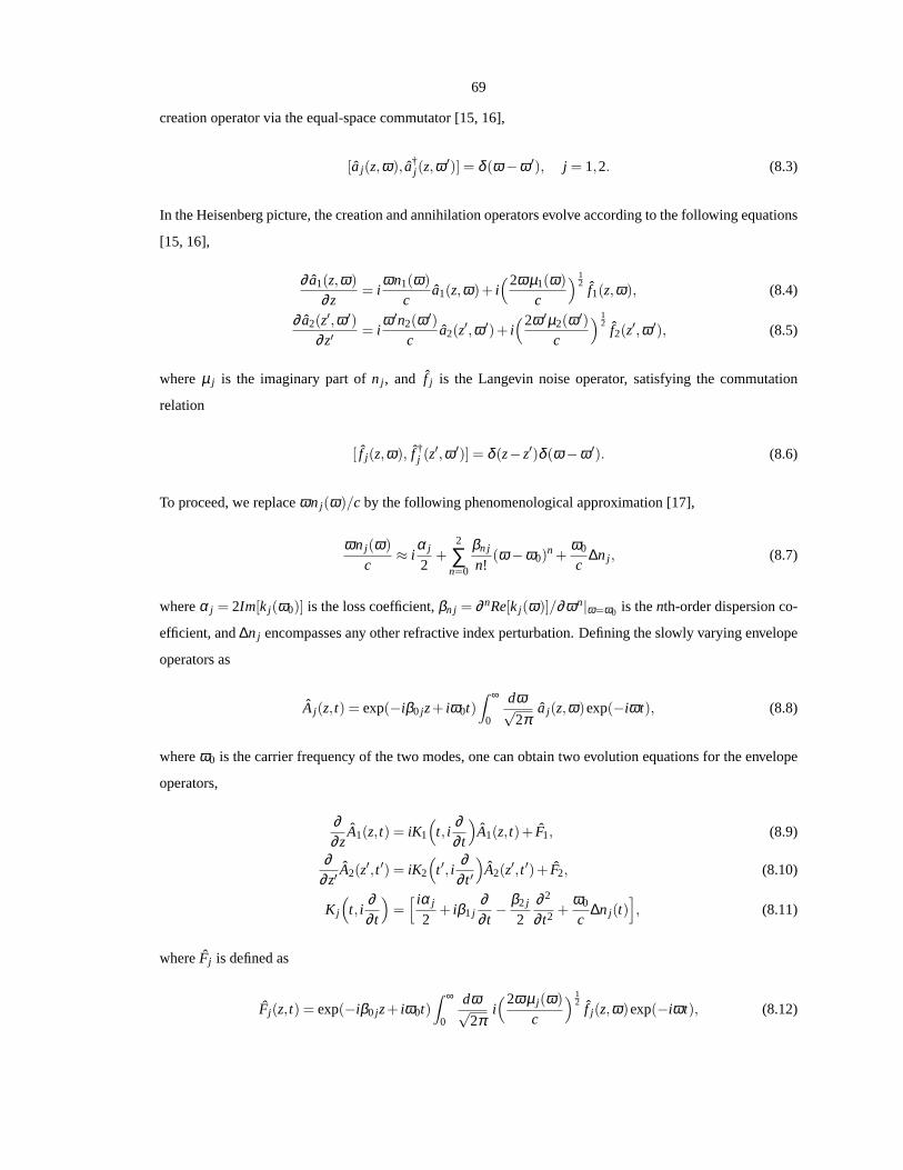
69
creation operator via the equal-space commutator [15, 16],
[a j(z,ω), a†j (z,ω
′)] = δ (ω −ω ′), j = 1,2. (8.3)
In the Heisenberg picture, the creation and annihilation operators evolve according to the following equations
[15, 16],
∂ a1(z,ω)
∂ z= i
ωn1(ω)
ca1(z,ω)+ i
(2ωµ1(ω)
c
) 12
f1(z,ω), (8.4)
∂ a2(z′,ω ′)∂ z′
= iω ′n2(ω ′)
ca2(z
′,ω ′)+ i(2ω ′µ2(ω ′)
c
) 12
f2(z′,ω ′), (8.5)
whereµ j is the imaginary part ofn j , and f j is the Langevin noise operator, satisfying the commutation
relation
[ f j(z,ω), f †j (z
′,ω ′)] = δ (z− z′)δ (ω −ω ′). (8.6)
To proceed, we replaceωn j(ω)/c by the following phenomenological approximation [17],
ωn j(ω)
c≈ i
α j
2+
2
∑n=0
βn j
n!(ω −ω0)
n +ω0
c∆n j , (8.7)
whereα j = 2Im[k j(ω0)] is the loss coefficient,βn j = ∂ nRe[k j(ω)]/∂ωn|ω=ω0 is thenth-order dispersion co-
efficient, and∆n j encompasses any other refractive index perturbation. Defining the slowly varying envelope
operators as
A j(z, t) = exp(−iβ0 jz+ iω0t)∫ ∞
0
dω√2π
a j(z,ω)exp(−iωt), (8.8)
whereω0 is the carrier frequency of the two modes, one can obtain two evolution equations for the envelope
operators,
∂∂ z
A1(z, t) = iK1
(
t, i∂∂ t
)
A1(z, t)+ F1, (8.9)
∂∂ z′
A2(z′, t ′) = iK2
(
t ′, i∂
∂ t ′
)
A2(z′, t ′)+ F2, (8.10)
K j
(
t, i∂∂ t
)
=[ iα j
2+ iβ1 j
∂∂ t
− β2 j
2∂ 2
∂ t2 +ω0
c∆n j(t)
]
, (8.11)
whereFj is defined as
Fj(z, t) = exp(−iβ0 jz+ iω0t)∫ ∞
0
dω√2π
i(2ωµ j(ω)
c
) 12
f j(z,ω)exp(−iωt), (8.12)

70
andK j is the complex wavenumber for the slowly varying envelope.∆n j can explicitly depend on time, if the
perturbation is much slower than the optical-frequency oscillation so that an adiabatic approximation can be
made, such as in an electro-optic modulator.
We now define the two-photon probability amplitudes as
ψ12(z, t,z′, t ′) = 〈0|A1(z, t)A2(z
′, t ′)|Ψ〉, (8.13)
ψ11(z, t,z′, t ′) =
1√2〈0|A1(z, t)A1(z
′, t ′)|Ψ〉, (8.14)
ψ22(z, t,z′, t ′) =
1√2〈0|A2(z, t)A2(z
′, t ′)|Ψ〉. (8.15)
The physical significance of each amplitudeψ jk is that its magnitude squared gives the probability density,
Pjk, of coincidentally measuring one photon in modej at (z, t) and another photon in modek at (z′, t ′),
Pjk(z, t,z′, t ′) = |ψ jk(z, t,z
′, t ′)|2. (8.16)
Temporal entanglement is defined as the irreducibility of|ψ12|2 into a product of one-photon amplitudes in the
form of a(t)b(t ′). This means that the probability of detecting a photon in mode 1 at timet is correlated to the
probability of detecting a photon in mode 2 att ′. The most popular ways of generating entangled photons are
spontaneous parametric down conversion [18] and four-wavemixing [19], where the wave mixing geometry
and the spatiotemporal profile of the pump beam determine theinitial ψ12.
To obtain the evolution equations for the two-photon amplitudeψ12(z, t,z′, t ′) in the Schrodinger picture,
we employ the same trick as in Ref. [2]. First we multiply Eq. (8.9) withA2(z′, t ′) and Eq. (8.10) withA1(z, t)
to produce two equations,
∂∂ z
A1(z, t)A2(z′, t ′) = iK1
(
t, i∂∂ t
)
A1(z, t)A2(z′, t ′)+ F1A2, (8.17)
∂∂ z′
A1(z, t)A2(z′, t ′) = iK2
(
t ′, i∂
∂ t ′
)
A1(z, t)A2(z′, t ′)+ F2A1. (8.18)
Using the definition ofψ12 in Eq. (8.13) and assuming that the thermal reservoirs are inthe vacuum state so
that the Langevin operators evaluate to zero when applied tothe wavefunction [20], a pair of equations in
terms ofψ12 are derived,
∂∂ z
ψ12(z, t,z′, t ′) = iK1
(
t, i∂∂ t
)
ψ12(z, t,z′, t ′), (8.19)
∂∂ z′
ψ12(z, t,z′, t ′) = iK2
(
t ′, i∂
∂ t ′
)
ψ12(z, t,z′, t ′). (8.20)
Equations (8.19) and (8.20) are the temporal version of the STS equations [2], including the effects of loss,

71
dispersion and phase modulation. They can also be written inthe frequency domain as
φ12(z,Ω,z′,Ω′) =∫ ∞
−∞dt∫ ∞
−∞dt ′ ψ12(z, t,z
′, t ′)×
exp(iΩt + iΩ′t ′), (8.21)
∂∂ z
φ12(z,Ω,z′,Ω′) = iK1
(1i
∂∂Ω
,Ω)
φ12(z,Ω,z′,Ω′), (8.22)
∂∂ z′
φ12(z,Ω,z′,Ω′) = iK2
(1i
∂∂Ω′ ,Ω
′)
φ12(z,Ω,z′,Ω′). (8.23)
For entangled photons, becauseψ12 or φ12 cannot be separated into a product of one-photon amplitudes,
distortions experienced in one arm can coherently add to thedistortions experienced in the other arm, leading
to various nonlocal quantum effects.
For example, considering group-velocity dispersion only,the outputφ12 is given by
φ12(z,Ω,z′,Ω′) = exp(
iβ11Ωz+ iβ12Ω′z′ +iβ21
2Ω2z+
iβ22
2Ω′2z′
)
φ12(0,Ω,0,Ω′). (8.24)
If the photons are initially entangled with negative frequency correlation,φ12(0,Ω,0,Ω′) can be approximated
by φ(Ω)δ (Ω+Ω′). Ignoring the unimportant linear spectral phase, the output is
φ12(z,Ω,z′,Ω′) = exp[ iΩ2
2(β21z+β22z′)
]
φ(Ω)δ (Ω+Ω′). (8.25)
Hence ifβ21z = −β22z′, the dispersion effects in both arms can nonlocally cancel each other, as originally
discovered by Franson [5].
8.3 Quantum temporal imaging
In the Schrodinger picture, the two-photon amplitude evolves under temporal effects. Since the entanglement
properties of the photons are contained in the two-photon amplitude, the Schrodinger picture allows one to
use the temporal effects to engineer the entanglement.
First, consider the evolution of the two-photon amplitude when one of the modes, say mode 1, is subject
to group-velocity dispersion,
∂ψ12
∂ z= −β11
∂ψ12
∂ t− iβ21
2∂ 2ψ12
∂ t2 , (8.26)
ψ12(L, t,z′, t ′) =
∫ ∞
−∞dτ b1(t − τ)ψ12(0,τ,z′, t ′), (8.27)
b1(t − τ) =( i
2πβ21L
) 12
exp[−i(t −β11L− τ)2
2β21L
]
. (8.28)
Group-velocity dispersion is well known to be analogous to Fresnel diffraction.

72
Next, consider a quadratic temporal modulation of refractive index imposed on mode 1 by a short or
traveling-wave electro-optic modulator,
∂ψ12
∂ z=
ik0∆n2(t − t0)2
2ψ12, (8.29)
ψ12(l, t,z′, t ′) = q(t)ψ12(0, t,z′, t ′), (8.30)
q(t) = exp[ ik0∆n2l
2(t − t0)
2]
. (8.31)
Quadratic temporal phase modulation is analogous to a lens.∆n2 is assumed to be a constant, andt0 is the
time delay of the modulation. Kerr effect by a copropagatingclassical pulse would also suffice.
Two dispersive elements with a quadratic phase modulator inbetween form a temporal imaging system,
which has been well studied in the classical domain [21]. Suppose that the photon in mode 1 propagates
through the first dispersive element, with an effective dispersion coefficientβ21 and effective lengthL, then
passes through a time lens with refractive index modulation∆n2(t − t0)2/2, and finally propagates through
the second dispersive element, with an effective dispersion coefficientβ ′21 and effective lengthL′. The output
two-photon amplitude can be expressed in terms of the input as
ψ12(z, t,z′, t ′) =
∫ ∞
−∞dτ∫ ∞
−∞dτ ′ b′1(t − τ ′)q(τ ′)b1(τ ′− τ)ψ12(0,τ,z′, t ′), (8.32)
b′1(t − τ ′) =( i
2πβ ′21L′
) 12
exp[−i(t −β ′
11L′− τ ′)2
2β ′21L′
]
. (8.33)
When the “lens law” for the time domain is satisfied,
1β21L
+1
β ′21L′ = k0∆n2l, (8.34)
the impulse response of the system becomes
h(t,τ) =∫ ∞
−∞dτ ′ b′1(t − τ ′)q(τ ′)b1(τ ′− τ) (8.35)
=i
2π√
β21Lβ ′21L′ exp
[−i(t −β ′11L′)2
2β ′21L′
]
×
exp[−i(τ +β11L)2
2β21L
]
∫ ∞
−∞dτ ′ P(
τ ′
Ta)×
exp[
i( t −β ′
11L′
β ′21L′ +
τ +β11Lβ21L
− k0∆n2lt0)
τ ′]
, (8.36)
whereP(τ ′/Ta) is the normalized temporal aperture function of the time lens that can be used to describe
any deviation of the actual temporal phase modulation from the ideal quadratic profile, such as truncation or

73
higher-order phase modulation, andTa is the aperture width. If
Ta >>β2LT0
, (8.37)
whereT0 is the smallest feature size ofψ12 along thet axis, the integral in Eq. (8.36) can be approximated by
a delta function. We then arrive at the input-output relation for the two-photon amplitude,
ψ12(z, t,z′, t ′) =
1√M
ψ12(0,t − td
M,z′, t ′), (8.38)
td = β ′11L′ +Mβ11L+(1−M)t0, (8.39)
M = −β ′21L′
β21L, (8.40)
where an unimportant quadratic phase factor is omitted,td is the time delay of the system, andM is the
magnification, which can be positive or negative depending on the signs ofβ2 andβ ′2.
Figure 8.1: Two-dimensional sketches of the two-photon probability amplitude before and after one of thephotons is time-reversed. Uncertainty in arrival time difference is transformed to uncertainty in mean arrivaltime.
The most interesting case is whenM = −1, and one of the photons is time-reversed. If the two photons
are initially entangled with positive time correlation,ψ12 can be written as
ψ12(0, t,z′, t ′) = a(t)b(t − t ′), (8.41)
whereb is assumed to be much sharper thana. After photon 1 has passed through the temporal imaging
system withM = −1,
ψ12(z, t,z′, t ′) = a(td − t)b(td − t − t ′). (8.42)
The photons hence become anticorrelated in time. See Fig. 8.1 for an illustration of this process. Since
most conventional two-photon sources generate positive time correlation, but negative time correlation is
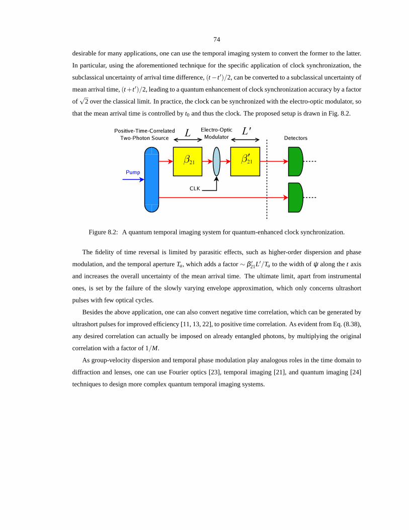
74
desirable for many applications, one can use the temporal imaging system to convert the former to the latter.
In particular, using the aforementioned technique for the specific application of clock synchronization, the
subclassical uncertainty of arrival time difference,(t− t ′)/2, can be converted to a subclassical uncertainty of
mean arrival time,(t +t ′)/2, leading to a quantum enhancement of clock synchronization accuracy by a factor
of√
2 over the classical limit. In practice, the clock can be synchronized with the electro-optic modulator, so
that the mean arrival time is controlled byt0 and thus the clock. The proposed setup is drawn in Fig. 8.2.
Figure 8.2: A quantum temporal imaging system for quantum-enhanced clock synchronization.
The fidelity of time reversal is limited by parasitic effects, such as higher-order dispersion and phase
modulation, and the temporal apertureTa, which adds a factor∼ β ′21L′/Ta to the width ofψ along thet axis
and increases the overall uncertainty of the mean arrival time. The ultimate limit, apart from instrumental
ones, is set by the failure of the slowly varying envelope approximation, which only concerns ultrashort
pulses with few optical cycles.
Besides the above application, one can also convert negative time correlation, which can be generated by
ultrashort pulses for improved efficiency [11, 13, 22], to positive time correlation. As evident from Eq. (8.38),
any desired correlation can actually be imposed on already entangled photons, by multiplying the original
correlation with a factor of 1/M.
As group-velocity dispersion and temporal phase modulation play analogous roles in the time domain to
diffraction and lenses, one can use Fourier optics [23], temporal imaging [21], and quantum imaging [24]
techniques to design more complex quantum temporal imagingsystems.
75
8.4 Two photons in two linearly coupled modes
Suppose that the two modes are now coupled to each other, via,for example, a beam splitter or a fiber coupler.
Equations (8.9) and (8.10) become coupled-mode equations,
( ∂∂ z
− iK1
)
A1 = iκ(z)A2 + F1, (8.43)
( ∂∂ z′
− iK′2
)
A′2 = iκ∗(z′)A′
1 + F ′2, (8.44)
whereκ is the coupling coefficient, and for simplicity the couplingis assumed to be codirectional. The
primes denote the evaluations of the functions at(z′, t ′). Any phase mismatch can be incorporated intoκ as a
z-dependent phase.
Procedures similar to those in Sec. 8.2 produce four coupledequations forψ11, ψ22, andψ12,
( ∂∂ z
− iK1
)√2ψ11(z, t,z
′, t ′) = iκψ12(z′, t ′,z, t), (8.45)
( ∂∂ z′
− iK′2
)√2ψ22(z, t,z
′, t ′) = iκ∗′ψ12(z′, t ′,z, t), (8.46)
( ∂∂ z
− iK1
)
ψ12(z, t,z′, t ′) = iκ
√2ψ22(z, t,z
′, t ′), (8.47)
( ∂∂ z′
− iK′2
)
ψ12(z, t,z′, t ′) = iκ∗′√2ψ11(z, t,z
′, t ′). (8.48)
Any pair of Eqs. (8.46) and (8.47) or Eqs. (8.45) and (8.48) can be combined to yield a single equation for
ψ12,
( ∂∂ z
− iK1
)( ∂∂ z′
− iK′2
)
ψ12(z, t,z′, t ′) = −κ(z)κ∗(z′)ψ12(z
′, t ′,z, t). (8.49)
Equation (8.49) allows one to calculate the coupled-mode propagation of two photons in terms ofψ12 only,
given the initial conditions ofψ12, ψ11, andψ22. ψ11 andψ22 can then be obtained from Eqs. (8.47) and
(8.48) afterψ12 is calculated.
To obtain some insight into Eq. (8.49), consider only constant mode coupling, so that Eq. (8.49) becomes
∂∂ z
∂∂ z′
ψ12(z, t,z′, t ′) = −κ2ψ12(z
′, t ′,z, t). (8.50)
The solution is
ψ12(z, t,z′, t ′) = cos(κz)cos(κz′)ψ12(0, t,0, t ′)−sin(κz)sin(κz′)ψ12(0, t ′,0, t)+
isin(κz)cos(κz′)√
2ψ22(0, t,0, t ′)+ icos(κz)sin(κz′)√
2ψ11(0, t,0, t ′). (8.51)
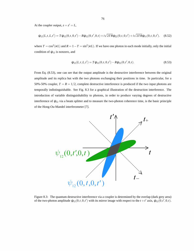
76
At the coupler output,z = z′ = L,
ψ12(L, t,L, t ′) = T ψ12(0, t,0, t ′)−Rψ12(0, t ′,0, t)+ i√
2T Rψ22(0, t,0, t ′)+ i√
2T Rψ11(0, t,0, t ′). (8.52)
whereT = cos2(κL) andR = 1−T = sin2(κL). If we have one photon in each mode initially, only the initial
condition ofψ12 is nonzero, and
ψ12(L, t,L, t ′) = T ψ12(0, t,0, t ′)−Rψ12(0, t ′,0, t). (8.53)
From Eq. (8.53), one can see that the output amplitude is the destructive interference between the original
amplitude and its replica but with the two photons exchanging their positions in time. In particular, for a
50%-50% coupler,T = R = 1/2, complete destructive interference is produced if the twoinput photons are
temporally indistinguishable. See Fig. 8.3 for a graphicalillustration of the destruction interference. The
introduction of variable distinguishability to photons, in order to produce varying degrees of destructive
interference ofψ12 via a beam splitter and to measure the two-photon coherence time, is the basic principle
of the Hong-Ou-Mandel interferometer [7].
Figure 8.3: The quantum destructive interference via a coupler is determined by the overlap (dark grey area)of the two-photon amplitudeψ12(0, t,0, t ′) with its mirror image with respect to thet + t ′ axis,ψ12(0, t ′,0, t).
77
8.5 Two photons in many modes
If the two photons are optically coupled to more than two modes, such as four modes for two polarizations
in each of the two propagation directions, orN modes in an array ofN fibers coupled to each other, one in
general needsN(N +1)/2 two-photon amplitudes to describe the system. The propagation of the amplitudes
in many modes is described by the following,
( ∂∂ z
− iK j
)√
1+δ jkψ jk(z, t,z′, t ′) = i ∑
l 6= j
κ jl
√
1+δlkψlk(z, t,z′, t ′), (8.54)
where
ψ jk(z, t,z′, t ′) = ψk j(z
′, t ′,z, t), κ jk = κ∗k j. (8.55)
Further simplications can also be made if any of the couplingterms is zero.
For example, let there be four modes; mode 1 corresponds to arm 1 with x polarization, mode 2 corre-
sponds to arm 2 withx polarization, mode 3 corresponds to arm 1 withy polarization, and mode 4 corresponds
to arm 2 withy polarization. If only the same polarizations are coupled, the two-photon equations are
∂∂z −iκx 0 0
−iκx∂∂z 0 0
0 0 ∂∂z −iκy
0 0 −iκy∂∂z
√2ψ11 ψ12 ψ13 ψ14
ψ21√
2ψ22 ψ23 ψ24
ψ31 ψ32√
2ψ33 ψ34
ψ41 ψ42 ψ43√
2ψ44
= 0. (8.56)
The following solution for the orthogonally polarized amplitudes can be obtained:
ψ13(L, t,L, t ′)
ψ24(L, t,L, t ′)
ψ14(L, t,L, t ′)
ψ23(L, t,L, t ′)
=
√
TxTy −√
RxRy i√
TxRy i√
TyRx
−√
RxRy√
TxTy i√
TyRx i√
TxRy
i√
TxRy i√
TyRx√
TxTy −√
RxRy
i√
TyRx i√
TxRy −√
RxRy√
TxTy
ψ13(0, t,0, t ′)
ψ24(0, t,0, t ′)
ψ14(0, t,0, t ′)
ψ23(0, t,0, t ′)
, (8.57)
whereTx,y = cos2(κx,yL) andRx,y = 1−Tx,y. In particular, if only the initial condition ofψ14 is nonzero,
ψ13(L, t,L, t ′) = i√
TxRyψ14(0, t,0, t ′), (8.58)
ψ24(L, t,L, t ′) = i√
TyRxψ14(0, t,0, t ′), (8.59)
ψ14(L, t,L, t ′) =√
TxTyψ14(0, t,0, t ′), (8.60)
ψ23(L, t,L, t ′) = −√
RxRyψ14(0, t,0, t ′). (8.61)
The singlet state for orthogonally polarized photons is produced ifTx = Ty = 1/2 [25].
78
8.6 Four-wave mixing
As envisioned by Lukinet al., the third-order nonlinear effects among two photons can become significant in
a coherently prepared atomic gas [4]. The coupled-mode equations (8.43) and (8.44) then become nonlinear,
( ∂∂ z
− iK1
)
A1 = iκA2 + iγA†1A1A1 + iηA†
2A2A1 + iχA2A2A†1 + F1, (8.62)
( ∂∂ z′
− iK′2
)
A′2 = iκ∗′A′
1 + iγA′†2A′
2A′2 + iηA′†
1A′1A′
2 + iχ∗′A′1A′
1A′†2 + F ′
2, (8.63)
whereγ is the self-phase modulation coefficient,η is the cross-phase modulation coefficient, andχ is the
four-wave mixing coefficient. If we define equal-space two-photon amplitudes as the following,
ψ jk(z, t, t′) = ψ jk(z, t,z, t
′), (8.64)
threelinear coupled-mode equations for the two-photon amplitudes can be derived,
( ∂∂ z
− iK1− iK′1
)√2ψ11 = iκψ21+ iγδ (t − t ′)
√2ψ11+ iχδ (t − t ′)
√2ψ22, (8.65)
( ∂∂ z
− iK2− iK′2
)√2ψ22 = iκ∗ψ21+ iγδ (t − t ′)
√2ψ22+ iχ∗δ (t − t ′)
√2ψ11, (8.66)
( ∂∂ z
− iK1− iK′2
)
ψ12 = iκ∗√2ψ11+ iκ√
2ψ22+ iηδ (t − t ′)ψ12. (8.67)
The advantage of the Schrodinger picture is most evident here; whereas in the Heisenberg picture one needs to
solve nonlinear coupled-mode operator equations such as Eqs. (8.62) and (8.63), in the Schrodinger picture,
one only needs to solve linear equations such as Eqs. (8.65) to (8.67), which are similar to the configuration-
space model applied to the quantum theory of solitons [1, 26].
The delta functionδ (t − t ′) couples the two subspaces ofψ12(z, t, t ′), so entanglement can emerge from
unentangled photons [4]. To see this effect, assume that we only have four-wave mixing, so that Eq. (8.67)
becomes
∂∂ z
ψ12(z, t, t′) = iηδ (t − t ′)ψ12(z, t, t
′), (8.68)
which yields
ψ12(L, t, t ′) = exp[iηLδ (t − t ′)]ψ12(0, t, t ′). (8.69)
If the nonlinearity has a finite bandwidth∆ω, the delta function in time should be replaced by a finite-

79
bandwidth function, for example a sinc function,
ψ12(L, t, t ′) = exp iηL
π(t − t ′)sin[∆ω
2(t − t ′)
]
ψ12(0, t, t ′). (8.70)
Eq. (8.70) is the exact solution of the two-photon amplitudeunder the cross-phase modulation effect, while
Eq. (7) in Ref. [4], presumably derived in the Heisenberg picture, is only correct in the first-order. As
ψ12(L, t, t ′) cannot be written as a product of one-photon amplitudes evenif the two photons are initially
unentangled, entanglement is generated. The physical interpretation is that the two input photons act as pump
photons to the spontaneous four-wave mixing process and areannihilated to generate two new entangled
photons.
Unlike temporal imaging techniques, which can only manipulate the two-photon amplitude along the
horizontal axist or the vertical axist ′, cross-phase modulation allows some manipulation of the two-photon
amplitude along the diagonal time-difference axis,t − t ′. Unfortunately, cross-phase modulation by itself
cannot generate any temporal correlation, as it only imposes a phase on the two-photon temporal amplitude.
In order to have more control along thet− t ′ axis, one can combine the effects of cross-phase modulationand
dispersion, as shown in the following section.
8.7 Two-photon vector solitons
In this section we study a toy example, namely, a soliton formed by two photons in orthogonal polarizations
exerting cross-phase modulation on each other [17]. Although similar studies of two photons in the same
mode under the self-phase modulation effect have been performed in Refs. [8], cross-phase modulation offers
the distinct possibility of entangling two photons in different modes.
Consider the case in which two polarizations have the same group-velocity dispersion, so thatβ21 = β22 =
β2, and there is one photon in each polarization. The evolutionequation forψ12(z, t, t ′) is
( ∂∂ z
+β11∂∂ t
+β12∂
∂ t ′
)
ψ12 =[
− iβ2
2
( ∂ 2
∂ t2 +∂ 2
∂ t ′2
)
+ iηδ (t − t ′)]
ψ12. (8.71)
Defining time coordinates in a moving frame,
τ = t − β1z, τ ′ = t ′− β1z, (8.72)
β1 =β11+β12
2, ∆ =
β11−β12
2, (8.73)
we obtain the following equation forψ12(z,τ,τ ′),
( ∂∂ z
+∆∂
∂τ−∆
∂∂τ ′)
ψ12 =[
− iβ2
2
( ∂ 2
∂τ2 +∂ 2
∂τ ′2)
+ iηδ (τ − τ ′)]
ψ12. (8.74)

80
Equation (8.74) is a simple linear Schrodinger equation, describing a two-dimensional “wavefunction” ψ12(z,τ,τ ′)
in a moving frame subject to a delta potential. To solve forψ12 explicitly, we define new time coordinates,
τ+ =τ + τ ′
2, τ− =
τ − τ ′
2, (8.75)
Eq. (8.74) then becomes
( ∂∂ z
+∆∂
∂τ−
)
ψ12 =[
− iβ2
4
( ∂ 2
∂τ2+
+∂ 2
∂τ2−
)
+iη2
δ (τ−)]
ψ12. (8.76)
As evident from Eq. (8.76), the cross-phase modulation effect only offers confinement ofψ12 along the time
difference (τ−) axis, but not the mean arrival time (τ+) axis.
The only bound-state solution ofψ12 is
ψ12(z,τ+,τ−) = exp[
− i(β2
4S2 +
∆2
β2
)
z]
exp(
−S|τ−|+ i2∆β2
τ−)
×∫ ∞
−∞
dΩ2π
φ(Ω)exp(
− iΩτ+ +iβ2
4Ω2z)
. (8.77)
The delta potential enforcesS to take on the following value,
S = − ηβ2
, (8.78)
whereη andβ2 must have opposite signs. The final solution ofψ12 in the frame ofτ andτ ′ is therefore
ψ12(z,τ,τ ′) = exp[
− i(η2/4+∆2
β2
)
z]
exp[
−∣
∣
∣
η2β2
∣
∣
∣|τ − τ ′|+ i∆β2
(τ − τ ′)]
×∫ ∞
−∞
dΩ2π
φ(Ω)exp[
− iΩ(τ + τ ′
2)+
iβ2
4Ω2z]
. (8.79)
The two-photon coherence time of a vector soliton is fixed, but the average arrival time is still subject to
dispersive spreading and becomes increasingly uncertain as the two photons propagate. See Fig. 8.4 for an
illustration. Hence, a two-photon vector soliton generates temporal entanglement with positive time corre-
lation as it propagates. Similar to the idea of soliton momentum squeezing [27], one can also adiabatically
changeη or β2 along the propagation axis to control independently the two-photon coherence time.
Notice that the center frequencies of the two photons are shifted slightly, by an amount of±∆/β2, to
compensate for their group-velocity mismatch, so that theycan copropagate at the average group velocity.
This is commonly known as soliton trapping [17].
If the nonlinearity has a finite bandwidth, then the potential becomes a finite-bandwidth function like the
one in Eq. (8.70), and multiple bound-state solutions can beobtained via conventional techniques of solving
the linear Schrodinger equation.

81
Figure 8.4: Quantum dispersive spreading of mean arrival time of a two-photon vector soliton. The cross-phase modulation effect only preserves the two-photon coherence time, giving rise to temporal entanglementwith positive time correlation. One can also manipulate thecoherence time independently by adiabaticallychanging the nonlinear coefficient along the propagation axis.
8.8 Conclusion
We have derived the general equations that govern the temporal evolution of two-photon probability ampli-
tudes in different coupled optical modes. The formalism inspires the concept of quantum temporal imaging,
which can manipulate the temporal entanglement of photons via conventional imaging techniques. The the-
ory also offers an intuitive interpretation of two-photon entanglement evolution, as demonstrated by the exact
solution of a two-photon vector soliton. To conclude, we expect the proposed formalism to be useful for
many quantum signal processing and communication applications.
82
Bibliography
[1] Y. Lai and H. A. Haus, Phys. Rev. A40, 844 (1989);40, 854 (1989).
[2] B. E. A. Saleh, M. C. Teich, and A. V. Sergienko, Phys. Rev.Lett. 94, 223601 (2005).
[3] E. Wolf, Nuovo Cimento12, 884 (1954).
[4] M. D. Lukin and A. Imamoglu, Phys. Rev. Lett.84, 1419 (2000).
[5] J. D. Franson, Phys. Rev. A45, 3126 (1992).
[6] A. M. Steinberg, P. G. Kwiat, and R. Y. Chiao, Phys. Rev. A45, 6659 (1992).
[7] C. K. Hong, Z. Y. Ou, and L. Mandel, Phys. Rev. Lett.59, 2044 (1987).
[8] R. Y. Chiao, I. H. Deutsch, and J. C. Garrison, Phys. Rev. Lett. 67, 1399 (1991); I. H. Deutsch, R. Y.
Chiao, and J. C. Garrison, Phys. Rev. Lett.693627 (1992).
[9] V. Giovannetti, S. Lloyd, and L. Maccone, Nature (London) 412, 417 (2001).
[10] V. Giovannetti, L. Maccone, J. H. Shapiro, and F. N. C. Wong, Phys. Rev. Lett.88, 183602 (2002).
[11] Z. D. Walton, M. C. Booth, A. V. Sergienko, B. E. A. Saleh,and M. C. Teich, Phys. Rev. A67, 053810
(2003).
[12] J. P. Torres, F. Macia, S. Carrasco, and L. Torner, Opt. Lett.30, 314 (2005).
[13] M. Tsang and D. Psaltis, Phys. Rev. A71, 043806 (2005).
[14] O. Kuzucu, M. Fiorentino, M. A. Albota, F. N. C. Wong, andF. X. Kartner, Phys. Rev. Lett.94, 083601
(2005).
[15] B. Huttner and S. M. Barnett, Phys. Rev. A46, 4306 (1992).
[16] R. Matloob, R. Loudon, S. M. Barnett, and J. Jeffers, Phys. Rev. A52, 4823 (1995).
[17] G. P. Agrawal,Nonlinear Fiber Optics (Academic Press, San Diego, 2001).
[18] M. H. Rubin, D. N. Klyshko, Y. H. Shih, and A. V. Sergienko, Phys. Rev. A50, 5122 (1994).

83
[19] M. Fiorentino, P. L. Voss, J. E. Sharping, and P. Kumar, IEEE Photon. Technol. Lett.14, 983 (2002).
[20] J. Jeffers and S. M. Barnett, Phys. Rev. A47, 3291 (1993).
[21] B. H. Kolner and M. Nazarathy, Opt. Lett.14, 630 (1989); B. H. Kolner, IEEE J. Quantum Electron.30,
1951 (1994).
[22] V. Giovannetti, L. Maccone, J. H. Shapiro, and F. N. C. Wong, Phys. Rev. A66, 043813 (2002).
[23] J. W. Goodman,Introduction to Fourier Optics (McGraw-Hill, Boston, 1996).
[24] A. F. Abouraddy, B. E. A. Saleh, A. V. Sergienko, and M. C.Teich, J. Opt. Soc. Am. B19, 1174 (2002).
[25] Z. Y. Ou, C. K. Hong, and L. Mandel, Opt. Commun.63, 118 (1987).
[26] P. L. Hagelstein, Phys. Rev. A54, 2426 (1996).
[27] J. M. Fini and P. L. Hagelstein, Phys. Rev. A66, 033818 (2002).

84
Chapter 9
Quantum temporal correlations andentanglement via adiabatic control ofvector solitons
9.1 Introduction
If an optical pulse consists ofN independent photons, then the uncertainty in the pulse center position is
the pulse width divided by√
N, the so-called standard quantum limit [1]. The ultimate limit permissible
by quantum mechanics, however, is determined by the Heisenberg uncertainty principle and is smaller than
the standard quantum limit by another factor of√
N, resulting in a quantum-enhanced accuracy useful for
positioning and clock synchronization applications [2]. To do better than the standard quantum limit, a
multiphoton state with positive frequency correlations and, equivalently, negative time correlations is needed
[2]. Consequently, significant theoretical [3, 4] and experimental [5] efforts have been made to create such
a nonclassical multiphoton state. All previous efforts were based on the phenomenon of spontaneous photon
pair generation in parametric processes, limitingN to 2 only. The resultant enhancement can only be regarded
as a proof of concept and is too small to be useful, considering that a large number of uncorrelated photons
can easily be obtained, with a standard quantum limit ordersof magnitude lower than the ultimate limit
achievable by two photons. It is hence much more desirable inpractice to be able to enhance the position
accuracy of a large number of photons. In this chapter, for the first time to the author’s knowledge, a scheme
that produces a multiphoton state with positive frequency correlations among an arbitrary number of photons
is proposed, thus enabling quantum position accuracy enhancement for macroscopic pulses as well. The
scheme set forth therefore represents a major step forward towards the use of quantum enhancement in future
positioning and clock synchronization applications.
The proposed scheme exploits the quantum properties of a vector soliton, in which photons in different
optical modes are bound together by the combined effects of group-velocity dispersion, self-phase modula-
tion, and cross-phase modulation [6]. A quantum analysis shows that the mean position of the photons in

85
a vector soliton is insensitive to the optical nonlinearities and only subject to quantum dispersive spreading,
while the separations among the photons are controlled by the balance between dispersion and nonlineari-
ties. These properties are in fact very similar to those of scalar solitons [7, 8], so the idea of adiabatically
compressing scalar solitons for momentum squeezing [9] canbe similarly applied to vector solitons. The
quantum dispersive spreading of the pulse center can simplybe compensated by classical dispersion manage-
ment, while the uncertainties in the relative frequencies among the photons can be reduced by adiabatically
increasing the dispersion or decreasing the nonlinearities, resulting in a multiphoton state with a transform-
limited mean-position uncertainty and positive frequencycorrelations. Given the past success of experiments
on scalar quantum solitons [10] and vector solitons [11], the scheme set forth should be realizable with cur-
rent technology. The formalism should apply to spatial vector solitons as well, so that the position accuracy
of an optical beam can be enhanced [12]. Moreover, the proposed scheme is capable of creating Einstein-
Podolsky-Rosen (EPR) entanglement [13] among the positions of the pulses in a vector soliton, suggesting
that the vector soliton effect, together with quantum temporal imaging techniques [4], may be used for general
continuous-variable quantum information processing [14].
For simplicity, only vector solitons with two optical modes, such as optical fiber solitons with two polar-
izations, are analytically investigated in this chapter. The results for two-mode vector solitons are represen-
tative and can be naturally extended to multimode vector solitons, such as those studied in Refs. [15].
9.2 Theory
9.2.1 Formalism
Two-mode vector solitons are classically described by the following coupled nonlinear Schrodinger equations
[6],
i∂U∂ t
= −b∂ 2U∂ z2 +2c(|U |2 +B|V |2)U, (9.1)
i∂V∂ t
= −b∂ 2V∂ z2 +2c(|V |2 +B|U |2)V, (9.2)
whereU andV are complex envelopes of the two polarizations, assumed to have identical group velocities and
group-velocity dispersion,t is the propagation time,z is the longitudinal position coordinate in the moving
frame of the pulses,b is the group-velocity dispersion coefficient,c is the self-phase modulation coefficient,
andBc is the cross-phase modulation coefficient. For example,B = 2/3 for linear polarizations in a linearly
birefringent fiber [16],B = 2 for circular polarizations in an isotropic fiber [17], andB = 1 describes Manakov
solitons [18], realizable in an elliptically birefringentfiber [16]. For solitons to exist, it is required thatbc < 0.
86
Equations (9.1) and (9.2) can be quantized using the Hamiltonian below,
H = h∫
dz
[
b(∂U†
∂ z∂U∂ z
+∂V †
∂ z∂V∂ z
)
+ c(
U†U†UU +V †V †VV +2BU†V †UV)
]
, (9.3)
whereU andV are photon annihilation operators of the two polarizationsand the daggers denote the corre-
sponding creation operators. The Heisenberg equations of motion derived from Eq. (9.3) are analyzed using
perturbative techniques by Randet al. [19], who study the specific case of Manakov solitons, and by Lantz
et al. [20] and Leeet al. [21], who numerically investigate the photon number entanglement in higher-order
vector solitons. As opposed to these previous studies, in this chapter the exact quantum vector soliton solution
is derived in the Schrodinger picture, in the spirit of the scalar soliton analyses in Refs. [7, 8].
Since the Hamiltonian conserves photon number in each mode and the mean momentum, one can con-
struct simultaneous Fock and momentum eigenstates with theBethe ansatz [7, 22],
|n,m, p〉 =1√
n!m!
∫
dnx dmy fnmp(x1, ...,xn,y1, ...,ym)U†(x1)...U†(xn)V
†(y1)...V†(ym)|0〉, (9.4)
wheren andm are the photon numbers in the two polarizations andp is the mean momentum. Using the
Schrodinger equationE|Ψ〉 = H|Ψ〉, one obtains
Enmpfnmp(x1, ...,xn,y1, ...,ym)
= h
−b∑j
∂ 2
∂x2j
−b∑k
∂ 2
∂y2k
+2c[
∑i< j
δ (x j − xi)+ ∑l<k
δ (yk− yl )+B∑j,k
δ (x j − yk)]
×
fnmp(x1, ...,xn,y1, ...,ym). (9.5)
The soliton solution of Eq. (9.5) is
fnmp= Cnmexp
[
ip(
∑j
x j +∑k
yk
)
+c
2b
(
∑i< j
|x j − xi |+ ∑l<k
|yk− yl |+B∑j,k
|x j − yk|)
]
, (9.6)
whereCnm is a normalization constant. The energy can be calculated bysubstituting Eq. (9.6) into Eq. (9.5)
and is given by
Enmp= hbN p2− hc2
12b
[
n(n2−1)+m(m2−1)+3B2nm(n+m)]
, (9.7)
whereN = n + m. A physical state should contain a distribution of momentumstates, say a Gaussian, such

87
that the time-dependent multiphoton probability amplitude is now given by
fnm =∫
d p1
(2π∆p2)14
exp(
− p2
4∆p2 − ibN p2t)
fnmp (9.8)
= Cnm(8π)14
( ∆p1+4ibN∆p2t
) 12
exp
[
− ∆p2
1+4ibN∆p2t
(
∑j
x j +∑k
yk
)2]
× (9.9)
exp
[
c2b
(
∑i< j
|x j − xi |+ ∑l<k
|yk− yl |+B∑j,k
|x j − yk|)
]
, (9.10)
where∆p is determined by initial conditions and a constant energy term that does not affect the position
and momentum properties of a Fock state is omitted. Althougha more realistic soliton state should have
a superposition of Fock states resembling a coherent state [7], the Fock components of a coherent state for
N >> 1 have photon numbers very close to the mean value, so a Fock state should be able to adequately
represent the position and momentum properties of a coherent-state soliton.
9.2.2 Adiabatic soliton expansion
The multiphoton amplitudefnm consists of two components: a dispersive pulse-center component given
by Eq. (9.9) that governs the quantum dispersion of the mean photon position 1/N(∑ j x j + ∑k yk), and a
bound-state component given by Eq. (9.10) that fixes the distances among the photons via the attractive Kerr
potentials. Scalar solitons possess the same properties [7, 8], and it can be argued that all vector solitons with
any number of modes under the effects of group-velocity dispersion, self-phase modulation, and cross-phase
modulation must also be comprised of such two components. Itfollows that the momentum-space probability
amplitude, defined as theN-dimensional Fourier transform offnm, also consists of a mean momentum com-
ponent and a bound-state component that governs the relative momenta among the photons. If one increases
b or reducesc adiabatically, the multiphoton amplitude would remain in the same form, but with increased
uncertainties in the relative distances as well as reduced uncertainties in the relative momenta. More crucially,
the mean momentum uncertainty remains unaffected, leadingto a multiphoton state with positive momentum
correlations. The adiabatic approximation remains valid if the change happens over a propagation time scale
T >> h/|E(t = T )−E(t = 0)|, which is on the order of the initial soliton period divided by N. As optical
fiber solitons can typically propagate for a few soliton periods before loss becomes a factor, the desired adi-
abatic expansion should be realizable with current technology. In the following it is assumed for simplicity
that onlyc is adiabatically varied. Mathematically, in the limit of vanishingc, the bound-state component
becomes relatively flat, andfnm becomes solely governed by the pulse-center component,
fnm ∝ exp
[
− ∆p2
1+4ibN∆p2t
(
∑j
x j +∑k
yk
)2]
. (9.11)
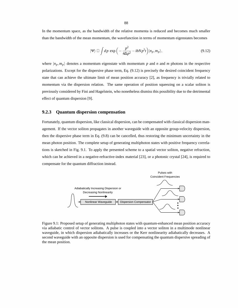
88
In the momentum space, as the bandwidth of the relative momenta is reduced and becomes much smaller
than the bandwidth of the mean momentum, the wavefunction interms of momentum eigenstates becomes
|Ψ〉 ∝∫
d p exp(
− p2
4∆p2 − ibN p2t)
|np,mp〉, (9.12)
where|np,mp〉 denotes a momentum eigenstate with momentump andn andm photons in the respective
polarizations. Except for the dispersive phase term, Eq. (9.12) is precisely the desired coincident frequency
state that can achieve the ultimate limit of mean position accuracy [2], as frequency is trivially related to
momentum via the dispersion relation. The same operation ofposition squeezing on a scalar soliton is
previously considered by Fini and Hagelstein, who nonetheless dismiss this possibility due to the detrimental
effect of quantum dispersion [9].
9.2.3 Quantum dispersion compensation
Fortunately, quantum dispersion, like classical dispersion, can be compensated with classical dispersion man-
agement. If the vector soliton propagates in another waveguide with an opposite group-velocity dispersion,
then the dispersive phase term in Eq. (9.8) can be cancelled,thus restoring the minimum uncertainty in the
mean photon position. The complete setup of generating multiphoton states with positive frequency correla-
tions is sketched in Fig. 9.1. To apply the presented scheme to a spatial vector soliton, negative refraction,
which can be achieved in a negative-refractive-index material [23], or a photonic crystal [24], is required to
compensate for the quantum diffraction instead.
Dispersion CompensatorNonlinear Waveguide
Pulses withCoincident Frequencies
...
Adiabatically Increasing Dispersion orDecreasing Nonlinearity
Figure 9.1: Proposed setup of generating multiphoton states with quantum-enhanced mean position accuracyvia adiabatic control of vector solitons. A pulse is coupledinto a vector soliton in a multimode nonlinearwaveguide, in which dispersion adiabatically increases orthe Kerr nonlinearity adiabatically decreases. Asecond waveguide with an opposite dispersion is used for compensating the quantum dispersive spreading ofthe mean position.

89
9.3 Temporal correlations among photons
In order to understand how the quantum vector soliton solution corresponds to a classical soliton in typical
experiments and how much adiabatic pulse expansion is needed to reach the ultimate quantum limit, consider
the specific case of a Manakov soliton, whereB = 1. Other vector solitons should have very similar properties
given the similarity of the solutions. If the photon position variables are re-indexed in the following new
notations,
z1, ...,zN = x1, ...,xn,y1, ...,ym, (9.13)
the multiphoton amplitude in Eqs. (9.9) and (9.10) becomes
fnm = Cnm(8π)1/4( ∆p
1+4ibN∆p2t
) 12
exp
[
− ∆p2
1+4ibN∆p2t
(
∑j
z j
)2+
c2b ∑
i< j|z j − zi |
]
. (9.14)
Intriguingly, this solution is exactly the same as the scalar soliton solution [7], or in other words, a Man-
akov soliton is quantum-mechanically equivalent to a scalar soliton. This equivalence explains the dis-
covery by Randet al. that the squeezing effect of a Manakov soliton has the same optimum as a scalar
soliton [19]. Moreover,Cnm can now be borrowed from the scalar soliton analysis and is given byCnm =
[(N −1)!|c/b|N−1/(2π)]1/2 [7]. The knowledge ofCnm allows one to calculate the correlations among the
photon positions using standard statistical mechanics techniques. An expression for⟨
∑i< j |z j − zi |⟩
can be
derived, and by symmetry,
⟨
|z j − zi |⟩
=1
N(N −1)
⟨
∑i< j
|z j − zi |⟩
=∣
∣
∣
2bNc
∣
∣
∣∼W0. (9.15)
As expected, the average absolute distance between any two photons is on the order of the classical soliton
pulse width,W0 ∼ |2b/(Nc)| [7]. Next, assume that the variance of the relative distanceis related to the
square of the average absolute distance by a parameterq,
⟨
|z j − zi |2⟩
= q⟨
|z j − zi |⟩2
=4qb2
N2c2 . (9.16)
While an explicit expression forq is hard to derive,q must only depend onN by dimensional analysis, must
be larger than 1 because⟨
|z j − zi |2⟩
≥⟨
|z j − zi |⟩2
, and is likely to be on the order of unity, as will be shown
later. Eq. (9.16) then gives
⟨
|z j − zi |2⟩
=⟨
z2j
⟩
−2⟨
ziz j⟩
+⟨
z2i
⟩
= 2⟨
z2j
⟩
−2⟨
ziz j⟩
, (9.17)
⟨
z2j
⟩
−⟨
ziz j⟩
=2qb2
N2c2 . (9.18)

90
Furthermore, the variance of∑ j z j is simply given by
⟨
(
∑j
z j
)2⟩
= N⟨
z2j
⟩
+N(N −1)⟨
ziz j⟩
= ∆z2, (9.19)
∆z2 =1
4∆p2 +4(
bN∆pt)2
. (9.20)
From Eqs. (9.18) and (9.19) the covariances can be obtained explicitly,
⟨
z2j
⟩
=∆z2
N2 +2q(N −1)b2
N3c2 ,⟨
ziz j⟩
=∆z2
N2 − 2qb2
N3c2 . (9.21)
A quantum soliton solution best resembles a classical initial condition with independent photons when the
initial covariance is zero,
⟨
ziz j⟩
t=0 =1
4N2∆p2 − 2qb2
N3c2
∣
∣
∣
t=0= 0, (9.22)
∆p =∣
∣
∣
√Nc√8qb
∣
∣
∣
t=0∼ 1
2√
NW0. (9.23)
Incidentally, the mean momentum uncertainty∆p is at the shot-noise level when the photons are initially
uncorrelated. This justifies the assumption thatq is on the order of unity. An initial condition with inde-
pendent photons would then mostly couple to a soliton state with ∆p given by Eq. (9.23), while coupling to
continuum states should be negligible. Adiabatically increasing|b/c| then makes⟨
ziz j⟩
negative and there-
fore introduces the necessary negative correlations amongthe photon positions. If the ratio between the final
and initial values of|b/c| is γ, for N >> 1 andγ <<√
N, the pulse bandwidth is reduced by a factor ofγ
according to the classical theory. The accuracy enhancement over the standard quantum limit for the same
reduced bandwidth is hence also given byγ in the regime of moderate expansion. The multiphoton state
becomes that given by Eqs. (9.11) and (9.12) and the ultimatelimit is reached only whenγ >>√
N.
9.4 Temporal entanglement between optical pulses
As the photons across different optical modes become correlated via the cross-phase modulation effect, en-
tanglement is expected among the pulse positions in a vectorsoliton. To estimate the magnitude of the
entanglement in terms of macroscopic position variables, consider again the case of Manakov solitons. Let
the pulse center coordinates of the respective polarizations beX andY , defined asX = 1/n∑nj=1 z j and
Y = 1/m∑Nk=m+1 zk. If there is an equal number of photons in each polarization such thatn = m = N/2, The
following statistics forX andY can be calculated using Eqs. (9.21),
⟨
(X +Y
2)2⟩
=∆z2
N2 ,
⟨
(X −Y
2)2⟩
=2qb2
N3c2 . (9.24)

91
Similar to a two-photon vector soliton [4], the mean position of the two pulses is affected by quantum dis-
persion, while the relative distance is bounded by the Kerr effect. For two initially uncorrelated pulses,
Eqs. (9.24) give the same value, but as the vector soliton propagates,∆z grows due to quantum dispersion,
leading to a positive temporal correlation between the two pulses. This correlation, however, does not re-
sult in the EPR paradox, as the joint spectrum in terms of the conjugate momenta with respect toX andY
does not change. If, on the other hand,b andc are adiabatically manipulated, then the nonlocal uncertainty
product⟨
(X −Y )2⟩⟨
(PX −PY)2⟩
, wherePX andPY are the conjugate momenta, can remain constant under
the adiabatic approximation while⟨
(X −Y )2⟩
and⟨
(PX −PY)2⟩
are varied, resulting in EPR entanglement.
Combined with quantum temporal imaging techniques, which are able to temporally reverse, compress, and
expand photons in each mode [4], adiabatic vector soliton control potentially provides a powerful way of
fiber-based continuous-variable quantum information processing [14].

92
Bibliography
[1] V. Giovannetti, S. Lloyd, and L. Maccone, Science306, 1330 (2004).
[2] V. Giovannetti, S. Lloyd, and L. Maccone, Nature (London) 412, 417 (2001).
[3] V. Giovannetti, L. Maccone, J. H. Shapiro, and F. N. C. Wong, Phys. Rev. Lett.88, 183602 (2002); Z. D.
Walton, M. C. Booth, A. V. Sergienko, B. E. A. Saleh, and M. C. Teich, Phys. Rev. A67, 053810 (2003);
J. P. Torres, F. Macia, S. Carrasco, and L. Torner, Opt. Lett.30, 314 (2005); M. Tsang and D. Psaltis, Phys.
Rev. A71, 043806 (2005).
[4] M. Tsang and D. Psaltis, Phys. Rev. A73, 013822 (2006).
[5] O. Kuzucu, M. Fiorentino, M. A. Albota, F. N. C. Wong, and F. X. Kartner, Phys. Rev. Lett.94, 083601
(2005).
[6] G. P. Agrawal,Nonlinear Fiber Optics (Academic Press, San Diego, 2001).
[7] Y. Lai and H. A. Haus, Phys. Rev. A40, 844 (1989);ibid. 40, 854 (1989).
[8] F. X. Kartner and H. A. Haus, Phys. Rev. A48, 2361 (1993); P. L. Hagelstein,ibid. 54, 2426 (1996).
[9] J. M. Fini and P. L. Hagelstein, Phys. Rev. A66, 033818 (2002).
[10] See, for example, A. Sizmann, Appl. Phys. B65, 745 (1997), and references therein; C. Silberhornet
al., Phys. Rev. Lett.86, 4267 (2001).
[11] See, for example, M. N. Islam, Opt. Lett.14, 1257 (1989); J. U. Kang, G. I. Stegeman, J. S. Aitchison,
and N. Akhmediev, Phys. Rev. Lett.76, 3699 (1996); Y. Barad and Y. Silberberg,ibid. 78, 3290 (1997); S.
T. Cundiff et al., ibid. 82, 3988 (1999).
[12] S. M. Barnett, C. Fabre, and A. Maitre, Eur. Phys. J. D22, 513 (2003).
[13] A. Einstein, B. Podolsky, and N. Rosen, Phys. Rev.47, 777 (1935).
[14] S. L. Braunstein and P. van Loock, Rev. Mod. Phys.77, 513 (2005).
[15] B. Crosignani and P. Di Porto, Opt. Lett.6, 329 (1981); F. T. Hioe, Phys. Rev. Lett.82, 1152 (1999).

93
[16] C. R. Menyuk, IEEE J. Quantum Electron.25, 2674 (1989).
[17] A. L. Berkhoer and V. E. Zakharov, Sov. Phys. JETP31, 486 (1970).
[18] S. V. Manakov, Sov. Phys. JETP38, 248 (1974).
[19] D. Rand, K. Steiglitz, and P. R. Prucnal, Phys. Rev. A71, 053805 (2005).
[20] E. Lantz, T. Sylvestre, H. Maillotte, N. Treps, and C. Fabre, J. Opt. B6, 295 (2004).
[21] R.-K. Lee, Y. Lai, and B. A. Malomed, Phys. Rev. A71, 013816 (2005).
[22] H. B. Thacker, Rev. Mod. Phys.53, 253 (1981).
[23] V. G. Veselago, Sov. Phys. Usp.10, 509 (1968); J. B. Pendry, Phys. Rev. Lett.85, 3966 (2000).
[24] C. Luo, S. G. Johnson, J. D. Joannopoulos, and J. B. Pendry, Phys. Rev. B65, 201104(R) (2002).

94
Chapter 10
Beating the spatial standard quantumlimits via adiabatic soliton expansionand negative refraction
10.1 Introduction
In many optical imaging applications, such as atomic force microscopy [1] and nanoparticle detection [2],
precise measurements of the displacement of an optical beamare required. It is hence important to know
what the fundamental limit on the accuracy of such measurements is placed by the laws of physics, and
how one can approach this limit in an experiment. It is now known that if an optical beam consists ofN
independent photons with wavelengthλ , then the minimum uncertainty in its spatial displacement is on the
order ofλ/√
N, the so-called standard quantum limit [3]. The ultimate uncertainty permissable by quantum
mechanics, however, is smaller than the standard quantum limit by another factor of√
N [3]. An experiment
that beats this standard quantum limit with nonclassical multimode light has already been demonstrated [4].
On the other hand, in other optical imaging applications, such as lithography, microscopy, and data storage,
detection of extremely small features of an object is desired. The feature size of an optical intensity pattern
cannot be smaller thanλ , due to the resolution limit [5]. Multiphoton absorption allows detection of smaller
feature sizes, and the minimum feature size of multiphoton absorption using a classical coherent light source
is on the order ofλ/√
N [6], which can be regarded as the standard quantum limit on the multiphoton
absorption feature size. Nonclassical light sources allowone to do better, and the ultimate limit is smaller
than the standard one by another factor of√
N [6, 7]. A proof-of-concept experiment of this resolution
enhancement has also been demonstrated [8]. In the time domain, very similar quantum limits on the position
accuracy of an optical pulse can be derived [9]. Given the striking similarities among the spatiotemporal
quantum limits, one expects them to be closely related to each other, yet the formalisms used to described
each of them are vastly different [3, 6, 7, 9], so a more general formalism applicable to all spatiotemporal
domains would greatly facilitate our understanding towards the spatiotemporal quantum enhancement effects.

95
In this chapter, we apply the temporal formalism used by Giovannettiet al. [9] to the spatial domain, and
show that the uncertainty in the beam displacement and the spot size of multiphoton absorption are in fact
closely related. Using this newly derived result, we demonstrate how one can generate arbitrary multiphoton
interference patterns with a continuous superposition of coincident momentum states. We further present
an unfortunate result, namely that the multiphoton absorption rate is reduced if the quantum lithography
resolution is enhanced, contrary to popular belief [6]. Finally, we take advantage of the general spatiotemporal
framework to show that the idea of adiabatic soliton expansion, previously proposed to beat the temporal
standard quantum limit [10], can also be used to beat both spatial standard quantum limits and approach the
ultimate limits with an arbitrary number of photons. The useof solitons is an attractive alternative to the more
conventional use of second-order nonlinearity for quantuminformation processing, because the soliton effect
bounds the photons together and allows a much longer interaction length for significant quantum correlations
to develop among the photons.
10.2 Formalism
ConsiderN photons with the same frequencyω and polarization that propagate in thex− z plane. A general
wavefunction that describes such photons is given by [11]
|Ψ〉 =1√N!
∫
dk1dk2...dkN φ(k1,k2, ...,kN)|k1,k2, ...,kN〉. (10.1)
where|k1, ...,kN〉 is the momentum eigenstate,k1, ...,kN specify the transverse wave vectors of the photons
along thex axis, andφ(k1, ...,kN) is defined as the multiphoton momentum probability amplitude. The
longitudinial wave vectors are all assumed to be positive. One can also define the corresponding quantities in
real space,
|x1, ...,xN〉 =
∫
dk1√2π
...dkN√
2πexp(−ik1x1− ...− ikNxN)|k1, ...,kN〉, (10.2)
ψ(x1, ...,xN) =∫
dk1√2π
...dkN√
2πφ(k1, ...,kN)exp(ik1x1 + ...+ ikNxN), (10.3)
|Ψ〉 =1√N!
∫
dx1...dxNψ(x1, ...,xN)|x1, ...,xN〉, (10.4)
whereψ(x1, ...,xN) is the multiphoton spatial probability amplitude.φ andψ are subject to normalization
conditions∫
dk1...dkN|φ |2 =∫
dx1...dxN|ψ|2 = 1, andφ and ψ must be symmetric under any exchange
of labels due to the bosonic nature of photons. The magnitudesquared ofψ gives the joint probability
96
distribution of the positions of the photons,
〈: I(x1)...I(xN) :〉 ∝1
N!〈Ψ|A†(x1)...A
†(xN)A(x1)...A(xN)|Ψ〉 (10.5)
= |ψ(x1, ...,xN)|2, (10.6)
whereA(xi) andA†(xi) are the spatial annihilation and creation operators, respectively. The statistical inter-
pretation ofψ is valid because we only consider photons that propagate in the positivez direction. The above
definition of a multiphoton state is more general than those used by other authors, in the sense that we allow
photons with arbitrary momenta, compared with the use of only one even spatial mode and one odd mode by
Fabreet al. [3], the use of only two discrete momentum states by Botoet al. [6], and the use of many discrete
momentum states by Bjork et al. [7].
The displacement of an optical beam can be represented by thefollowing operator,
X =1N
∫
dx xA†(x)A(x). (10.7)
Applying X to |x1, ...,xN〉 gives
X |x1, ...,xN〉 =
(
1N
N
∑i=1
xi
)
|x1, ...,xN〉, (10.8)
so the beam displacement can be intuitively regarded as the mean position of the photons under the statistical
interpretation. If we assume that⟨
X⟩
= 0 for simplicity, the displacement uncertainty is given by
⟨
X2⟩1/2=
∫
dx1...dxN
(
1N
N
∑i=1
xi
)2
|ψ(x1, ...,xN)|2
1/2
. (10.9)
It is often more convenient to use a different system of coordinates as follows [12],
X =1N
N
∑i=1
xi , ξi = xi −X , i = 1, ...,N −1, ξN = −N−1
∑i=1
ξi . (10.10)
X is therefore the “center-of-mass” coordinate that characterizes the overall displacement of the optical beam,
andξi ’s are relative coordinates. Defining a new probability amplitude in terms of these coordinates,
ψ ′(X ,ξ1, ...,ξN−1) = ψ(X +ξ1, ...,X +ξN), (10.11)

97
we obtain the following expression for the displacement uncertainty,
⟨
X2⟩1/2=
[
1N
∫
dXdξ1...ξN−1 X2|ψ ′(X ,ξ1, ...,ξN−1)|2]1/2
(10.12)
=⟨
X2⟩1/2, (10.13)
which is the marginal width ofψ ′ with respect toX .
On the other hand, the dosing operator ofN-photon absorption is [6]
⟨
: IN(x) :⟩
∝ |ψ(x,x, ...,x)|2 = |ψ ′(x,0, ...,0)|2, (10.14)
which is, intuitively, the probability distribution of allN photons arriving at the same placex. Hence, de-
signing a specified multiphoton interference pattern in quantum lithography is equivalent to engineering the
conditional probability distribution|ψ ′(X ,0, ...,0)|2. In particular, the spot size of multiphoton absorption is
the conditional width ofψ ′ with respect toX ,
[
∫
dx x2⟨: IN(x) :⟩
]1/2
∝[
∫
dX X2|ψ ′(X ,0, ...,0)|2]1/2
(10.15)
=⟨
X2⟩1/2 |ξ1=...=ξN−1=0. (10.16)
Despite the subtle difference between the marginal width and the conditional width, ifψ ′ can be made sepa-
rable in the following way,
ψ ′(X ,ξ1, ...,ξN−1) = ψ(X)ψrel(ξ1, ...,ξN−1), (10.17)
then both widths are identical, and one can optimize the multiphoton state simultaneously for both applica-
tions.
The standard quantum limit on the uncertainty inX is obtained when the photons are spatially in-
dependent, such thatψ(x1, ...,xN) = f (x1)... f (xN). For example, if f (x) is a Gaussian given byf (x) ∝
exp(
−κ2x2
2
)
, then both the marginal and conditional uncertainties inX are
⟨
X2⟩1/2SQL=
⟨
X2⟩1/2SQL
∣
∣
∣
ξ1=...=ξN−1=0=
1√2Nκ
. (10.18)
Similar to the optimization of temporal position accuracy [9], the ultimate quantum limits on spatial displace-
ment accuracy and quantum lithography feature size are achieved with the following nonclassical state,
|Ψ〉 =∫
dkG(k)|k,k, ...,k〉. (10.19)

98
The momentum probability amplitude is then
φ(k1, ...,kN) = G(k1)δ (k1− k2)δ (k1− k3)...δ (k1− kN), (10.20)
which characterizesN photons with coincident momentum. The spatial amplitude isthus given by
ψ ′(X ,ξ1, ...,ξN) =∫
dk√2π
G(k)exp(iNkX) ≡ g(NX), (10.21)
which is a function ofX only and can be understood as a continuous superposition ofN-photon states, each
with an effective de Broglie wavelength equal to 2π/(Nk). The multiphoton interference pattern is therefore
trivially given by |g(NX)|2, the magnitude squared of the Fourier transform ofG(k). An arbitrary interference
pattern can hence be generated, if an appropriateG(k) can be engineered. This approach of designing the
multiphoton interference pattern should be compared with the less direct approaches by the use of discrete
momentum states [6, 7]. With the resolution limit,G(k) is zero for|k|> 2π/λ , so given the Fourier transform
relation betweenG(k) andg(NX), the minimum feature size of multiphoton interference is onthe order of
λ/N.
To compare the ultimate uncertainty inX with the standard quantum limit, letG(k) be a Gaussian given
by G(k) ∝ exp(
− k2
2κ2
)
, then the uncertainty inX becomes
⟨
X2⟩1/2UQL =
1√2Nκ
, (10.22)
which is smaller than the standard quantum limit, Eq. (10.18), by another factor of√
N, as expected.
10.3 Multiphoton absorption rate of nonclassical states
Let us recall Botoet al.’s heuristic argument concerning the multiphoton absorption rate of entangled photons.
They claim that, because entangled photons tend to arrive atthe same place at the same time, the multiphoton
absorption rate must be enhanced [6]. If photons tend to arrive at the same place, then the uncertainty in
their relative positions must be small. However, the spatial probability amplitude that achieves the ultimate
lithographic resolution, Eq. (10.21), is a function ofX only, which means that the uncertainty in the relative
positions is actually infinite. In general, any enhancementof resolution with respect toX must result in a
corresponding reduction in the bandwidths with respect to the relative positions, in order to maintain the
same maximum bandwidth. By the Heisenberg uncertainty principle, such photons must then have increased
uncertainty in their relative positions. Hence, Botoet al.’s argument manifestly does not hold for photons
with a quantum-enhanced lithographic resolution. In fact,the opposite is true: Although these photons have
a reduced uncertainty in their average position, they must have an increased uncertainty in their relative
positions, so they do not arrive at the same place very often,and the multiphoton absorption rate must be
99
reduced. To observe this fact, consider the total multiphoton absorption rate,
∫
dx⟨
: IN(x) :⟩
∝∫
dX |ψ ′(X ,0, ...,0)|2. (10.23)
Becauseψ ′ must satisfy the normalization condition,
1N
∫
dXdξ1...dξN|ψ ′(X ,ξ1, ...,ξN)|2 = 1, (10.24)
a larger uncertainty inξi ’s means that|ψ ′(X ,0, ...,0)|2 must be smaller, leading to a reduced multiphoton
absorption rate. Conversely, photons that tend to arrive together must have a larger uncertainty in where they
arrive, so an enhanced multiphoton absorption rate means that the quantum lithographic resolution must be
sacrificed. That said, one can still compensate for the reduction in the multiphoton absorption rate due to an
enhanced resolution in one dimension, by reducing the relative positions of the photons in the other unused
space and time dimensions.
10.4 Generating nonclassical states via the soliton effect
We now turn to the problem of producing the nonclassical multiphoton states for spatial quantum enhance-
ment. As we have established a general formalism that resembles the temporal one, schemes that produce
temporal quantum enhancement can be applied to the spatial domain as well. In particular, a scheme that
makes use of temporal solitons is recently proposed to enhance the temporal accuracy of an optical pulse
[10]. We here proceed to show how spatial solitons can be utilized to enhance the beam displacement ac-
curacy, as well as reduce the spot size of multiphoton absorption, beyond the standard quantum limits and
approaching the ultimate quantum limits.
Consider the Hamiltonian that describes the one-dimensional diffraction effect and Kerr nonlinearity,
H =∫
dx
[
−b∂ A†
∂x∂ A∂x
+ cA†A†AA
]
, (10.25)
whereb is the Fresnel diffraction coefficient, assumed to be positive, andc is the negative Kerr coefficient,
assumed to be negative, so thatb/c < 0 and solitons can exist under the self-focusing effect. Thesoliton
solution of the spatial amplitude forN photons under this Hamiltonian is [13]
ψ = C∫
dk√2π
G(k)exp
[
ik∑i
xi +c
2b ∑i< j
|xi − x j |− ibNk2t + ic2
12bN(N2−1)t
]
, (10.26)
whereC =√
(N −1)!|c/b|N−1/(2π) andG(k) is determined by the initial conditions. If initially the photons

100
are uncorrelated,G(k) can be approximated as [10]
G(k) ∝ exp(
− k2
2κ2
)
, κ =
∣
∣
∣
∣
√
N4q
cb
∣
∣
∣
∣
∼ 1√NW0
, (10.27)
whereq is a parameter on the order of unity [10], andW0 is the initial soliton beam width. The probability
amplitude can be written in terms of the center-of-mass and relative coordinate system defined in Eqs. (10.10)
as
ψ ′ = C∫
dk√2π
G(k)exp
[
iNkX +c2b ∑
i< j|ξi −ξ j |− ibNk2t + i
c12b
N(N2−1)t
]
, (10.28)
which is separable in the way described by Eq. (10.17), meaning that the conditional width and marginal
width with respect toX are identical. If we adiabatically reducec or increaseb, then we can reduce the
uncertainty in the relative momenta of the photons and increase the uncertainty in the relative positions [10].
Classically, we expect the soliton beam width to expand and the spatial bandwidth to be reduced, But the
most crucial difference in the quantum picture is that the center-of-mass coordinateX remains unaffected
during the adiabatic soliton expansion, apart from the quantum dispersion term−ibNk2t.
As pointed out in Ref. [10], the quantum dispersion term can be compensated if the soliton propagates in
a second medium with an opposite diffraction coefficientb′. Full compensation is realized when∫ T
0 b(t)dt =
−∫ T ′0 b′(t)dt, whereT is the propagation time in the first medium andT ′ is the propagation time in the second
medium. Negative refraction, realizable in a left-handed material [14] or a photonic crystal [15] for example,
is hence required in the second medium. Ideally the second medium should also have a Kerr coefficientc′
opposite to the final value ofc in the first medium, such thatc′ = −c(T ), so thatb′/c′ < 0 and the quantum
soliton maintains its shape, but in practicec′ = 0 would also suffice, because the momentum bandwidths
would remain unchanged in a linear medium while the quantum dispersion is being compensated.
In the limit of vanishingc/b in the first medium, the wavefunction would approach the ultimate multi-
photon state given by Eq. (10.21). However, the bandwidth ofG(k) is very low, on the order of 1/(√
NW0),
whereW0 is the initial soliton beam width, so the bandwidth ofG(k) is nowhere near the resolution limit and
the uncertainty inX is the same as the input beam. In order to reduce this uncertainty, one can put the beam
in a conventional imaging system [16] to recompress it, so that the output probability amplitude becomes
ψout =1√MN
ψin
(x1
M,
x2
M, ...,
xN
M
)
, (10.29)
whereM is the magnification factor. IfM is smaller than 1, each photon is spatially compressed, thus
reducing the ultimate quantum limit on the uncertainty inX . To illustrate, Fig. 10.1 shows a flowchart of the
whole quantum enhancement process and a simple example of what the spatial and momentum probability
amplitudes should look like in each step for two photons.

101
Figure 10.1: First row: schematics of the spatial quantum enhancement setup via adiabatic soliton expansion.Second row: sketches of the spatial probability amplitude,ψ(x1,x2), for an example of two photons in eachstep of the process. Third row: sketches of the momentum probability amplitude,φ(k1,k2). Consult text fordetails of each step of the process.
10.5 Conclusion
In conclusion, spatial quantum enhancement effects are studied under a general framework. A method of
generating arbitrary multiphoton interference pattern bythe use of a continuous superposition of coincident
momentum states is proposed. It is further shown that the multiphoton absorption rate is reduced if the
lithographic resolution is enhanced. Finally, the use of adiabatic soliton expansion and negative refraction is
proposed to beat the spatial standard quantum limits.

102
Bibliography
[1] C. A. J. Putman, B. G. De Grooth, N. F. Van Hulst, and J. Greve, J. Appl. Phys.72, 6 (1992).
[2] S. Kamimura, Appl. Opt.26, 3425 (1987).
[3] C. Fabre, J. B. Fouet, and A. Maitre, Opt. Lett.25, 76 (2000); S. M. Barnett, C. Fabre, and A. Maitre,
Eur. Phys. J. D22, 513 (2003).
[4] N. Treps, U. Andersen, B. Buchler, P. K. Lam, A. Maıtre, H.-A. Bachor, and C. Fabre, Phys. Rev. Lett.
88, 203601 (2002).
[5] M. Born and E. Wolf,Principles of Optics (Cambridge University Press, Cambridge, UK, 1999).
[6] A. N. Boto, P. Kok, D. S. Abrams, S. L. Braunstein, C. P. Williams, and J. P. Dowling, Phys. Rev. Lett.
85, 2733 (2000); P. Kok, A. N. Boto, D. S. Abrams, C. P. Williams,S. L. Braunstein, and J. P. Dowling,
Phys. Rev. A63, 063407 (2001).
[7] G. Bjork, L. L. Sanchez-Soto, and J. Soderholm, Phys. Rev. Lett.86, 4516 (2001), G. Bjork, L. L.
Sanchez-Soto, and J. Soderholm, Phys. Rev. A64, 013811 (2001).
[8] M. D’Angelo, M. V. Chekhova, and Y. Shih, Phys. Rev. Lett.87, 013602 (2001).
[9] V. Giovannetti, S. Lloyd, and L. Maccone, Nature (London) 412, 417 (2001).
[10] M. Tsang, e-print quant-ph/0603088 [submitted to Phys. Rev. Lett. ].
[11] L. Mandel and E. Wolf,Optical Coherence and Quantum Optics (Cambridge University Press, Cam-
bridge, UK, 1995).
[12] P. L. Hagelstein, Phys. Rev. A54, 2426 (1996).
[13] Y. Lai and H. A. Haus, Phys. Rev. A40, 844 (1989);ibid. 40, 854 (1989).
[14] V. G. Veselago, Sov. Phys. Usp.10, 509 (1968); J. B. Pendry, Phys. Rev. Lett.85, 3966 (2000).
[15] C. Luo, S. G. Johnson, J. D. Joannopoulos, and J. B. Pendry, Phys. Rev. B65, 201104(R) (2002).
[16] J. W. Goodman,Introduction to Fourier Optics (McGraw-Hill, Boston, 1996).
103
Chapter 11
Reflectionless evanescent waveamplification via two dielectric planarwaveguides
11.1 Introduction
Conventional optical imaging systems cannot resolve features smaller than the optical wavelength, because
the high-spatial-frequency modes that describe the subwavelength features are evanescent waves, which ex-
ponentially decay away from the object and do not propagate to the far field. Observing the evanescent waves
is therefore one of the most important yet formidable challenges in the field of optics, with important ap-
plications in optical lithography, data storage, and microscopy. Near-field scanning optical microscopy can
detect the evanescent waves [1], but it requires scanning, which may not be desirable for many applications.
A groundbreaking proposal by Pendry suggests that evanescent waves can be amplified without any reflection
in a negative-refractive-index slab [2], causing significant interest as well as controversy [3] in the mechanism
of evanescent wave amplification (EWA). On the practical side, the fabrication of a negative-refractive-index
material for optical frequencies is a challenging task, as it requires both negative permittivity and negative
permeability, the latter of which does not naturally occur in materials, and methods of implementing an ef-
fective negative refractive index [4, 5, 6] often introducesignificant loss detrimental to the EWA process.
As proposed by Pendry [2] and experimentally demonstrated by Fanget al. [7], a negative permittivity in a
metal slab can also amplify evanescent waves to some extent,but the thickness of the slab is limited by the
electrostatic approximation as well as loss. A simpler EWA scheme that utilizes less lossy materials would
thus be desirable.
Along this direction, Luoet al. propose that a photonic crystal slab can be used to amplify evanescent
waves [8], since evanescent waves with specific spatial frequencies can be coupled into the bound states of
the photonic crystal slab, and the buildup of the bound states produces an enhanced evanescent tail on the
other side of the slab. Apart from the difficulty in fabricating a three-dimensional photonic crystal for two-

104
dimensional imaging, the kind of EWA achieved by a photonic crystal slab is not ideal, because the buildup
of the bound states also creates enhanced reflected evanescent waves, causing multiple evanescent wave
reflections between the object and the photonic crystal. On the other hand, in order to obtain information
about the output evanescent waves on the image plane, energymust be extracted, and the only way for the
detector to “tell” the imaging system to give up energy is viaa reflected evanescent wave. In other words,
detection of an evanescent wave always creates a reflected evanescent wave, so there exist multiple reflections
between an imaging system and the detector as well. Since themagnitudes of evanescent wave transmission
and reflection coefficients can be larger than 1 or even infinite, multiple evanescent wave reflections can be
very significant and should not be ignored in the design of near-field imaging systems. An ideal near-field
imaging system should hence have 100% transmission as well as zero reflection,as if the imaging system is
not there and the object directly touches the image plane. This ideal behavior also allows multiple imaging
systems to be cascaded and a longer distance between the object and the detector.
In this chapter, the underlying physics of reflectionless evanescent wave amplification (REWA) by the
use of a negative-refractive-index slab is explained, and,using this knowledge, it is shown that evanescent
waves with specific spatial frequencies can be amplified without reflection simply by two dielectric planar
waveguides. Since loss in a dielectric can be orders of magnitude lower than metals or metamaterials, our
proposed scheme is the simplest way of experimentally demonstrating the intriguing phenomenon of REWA
and offers simple alternatives to the use of left-handed materials, surface plasmons, or photonic crystals for
near-field imaging applications.
11.2 Evanescent wave amplification
One of the most poorly understood aspects of Pendry’s proposal is that at the interface of ann = 1 material
and ann = −1 material, the transmission and reflection coefficients aretheoretically infinite [2]. Mathemati-
cally this indicates the presence of an unstable pole on the imaginary axis in the complex transverse-spatial-
frequency (s = ikx) plane, and physically the transmitted and reflected evanescent optical fields must therefore
increase linearly along a semi-infinite interface. This is hardly surprising if one recalls the well-known fact
that infinite scattering coefficients correspond to bound-state solutions, so the incoming evanescent waves are
simply resonantly coupled into the waveguide modes of the interface. The most peculiar aspect of Pendry’s
interface is that the scattering coefficients are always infinite, meaning that bound-state solutions exist for all
kx. This is not true for other waveguides, including photonic crystals [8], which have discrete bound states
with different discretekx’s. In particular, for ideal surface plasmons, only one bound state exists.
11.2.1 Evanescent wave amplification by one dielectric slab
First, consider a dielectric slab with thicknessa and refractive indexn1 in thex− y plane. Suppose that an
evanescent s-polarized wave with an electric field exponentially decaying along thez axis given byE0+ =

105
[0,1,0]exp(ikzz+ ikxx− iωt) impinges on the slab, wherekx is assumed to have subwavelength resolution, so
kx > ωn0/c, kz is determined by the dispersion relation, given bykz = i√
k2x − k2
0, k0 = ωn0/c, andn0 is the
refractive index of the surroundings. Considering the firstinterface betweenn0 andn1 only, the reflected wave
is r[0,1,0]exp(−ikzz+ ikxx− iωt), and the transmitted wave inside the slab ist[0,1,0]exp(ik′zz+ ikxx− iωt).
kx is the same on both sides of the interface, andk′z is given by the dispersion relationk′z =√
k21− k2
x, where
k1 = ωn1/c. k′z is hereafter assumed to be real for waveguide modes to exist.This restrictskx to be bounded
by the wave numbers in the two media,
k0 < kx < k1. (11.1)
The transmission and reflection coefficients across the firstinterface are given byt = 2kz/(kz + k′z) and
r = (kz− k′z)/(kz + k′z) respectively. Likewise, the scattering coefficients across the second interface are
t ′ = 2k′z/(k′z+ kz) andr′ = (k′z− kz)/(k′z+ kz). To obtain the total transmission,τ, across the slab, multiple
scattering events must be summed,
τ = t exp(ik′za)t ′ + t exp(ik′za)[r′exp(ik′za)]2t ′ + ... (11.2)
=tt ′exp(ik′za)
1− r′2exp(2ik′za). (11.3)
The total reflection coefficient can be obtained similarly,
Γ = r +tt ′r′exp(2ik′za)
1− r′2exp(2ik′za). (11.4)
Waveguide modes correspond to those with evanescent tails exponentially decaying away from the waveg-
uide. In other words, the total transmitted evanescent waveand the total reflected evanescent wave for the
waveguide modes can exist by themselves without any incoming waveE0+, or, mathematically speaking,τ
andΓ are infinity. This happens when
1− r′2exp(2ik′za) = 1−(k′z− kz
k′z+ kz
)2exp(2ik′za) = 0, (11.5)
which simply states that the accumulated phase in a round trip inside the waveguide must be multiples of 2π.
As bothkz andk′z depend onkx, Eq. (11.5) is an eigenvalue equation ofkx for the TE modes of the single
waveguide. A simple dielectric slab can hence achieve EWA due to the waveguide mode coupling resonances,
similar to a photonic crystal [8]. If only subwavelength features are concerned and all-angle negative refrac-
tion [9] is not needed, a complicated structure such as photonic crystal is not necessary. However, just like a
photonic crystal, the reflection coefficientΓ of a slab waveguide is also infinite, causing potential problems
with multiple reflections.
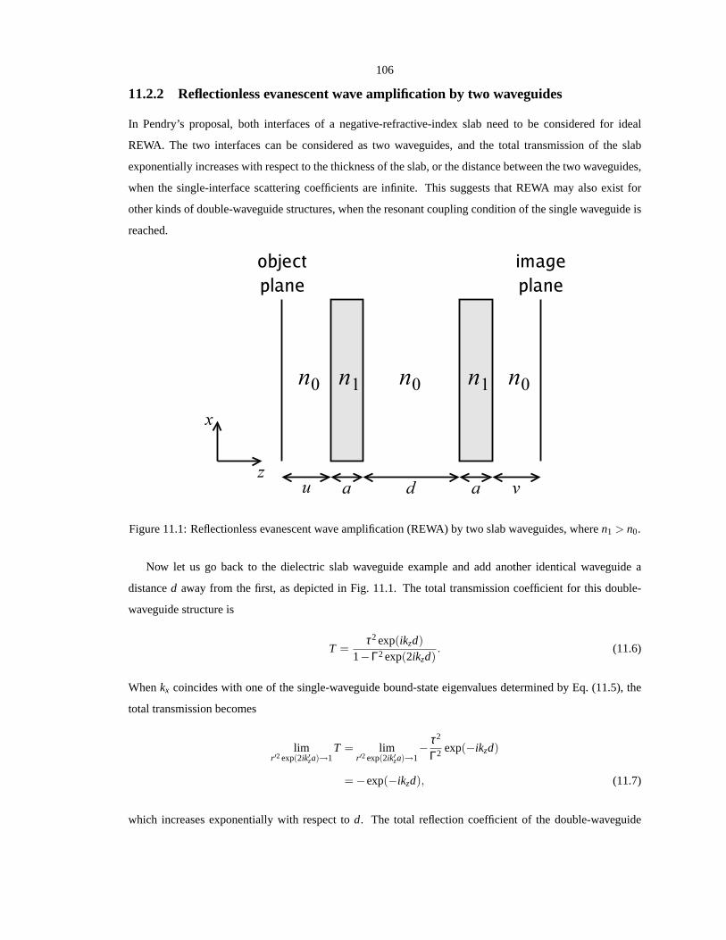
106
11.2.2 Reflectionless evanescent wave amplification by two waveguides
In Pendry’s proposal, both interfaces of a negative-refractive-index slab need to be considered for ideal
REWA. The two interfaces can be considered as two waveguides, and the total transmission of the slab
exponentially increases with respect to the thickness of the slab, or the distance between the two waveguides,
when the single-interface scattering coefficients are infinite. This suggests that REWA may also exist for
other kinds of double-waveguide structures, when the resonant coupling condition of the single waveguide is
reached.
Figure 11.1: Reflectionless evanescent wave amplification (REWA) by two slab waveguides, wheren1 > n0.
Now let us go back to the dielectric slab waveguide example and add another identical waveguide a
distanced away from the first, as depicted in Fig. 11.1. The total transmission coefficient for this double-
waveguide structure is
T =τ2exp(ikzd)
1−Γ2exp(2ikzd). (11.6)
Whenkx coincides with one of the single-waveguide bound-state eigenvalues determined by Eq. (11.5), the
total transmission becomes
limr ′2 exp(2ik′za)→1
T = limr ′2 exp(2ik′za)→1
− τ2
Γ2 exp(−ikzd)
= −exp(−ikzd), (11.7)
which increases exponentially with respect tod. The total reflection coefficient of the double-waveguide

107
structure is likewise given by
R = Γ+τ2Γexp(2ikzd)
1−Γ2exp(2ikzd), (11.8)
and in the limit ofkx being a bound-state eigenvalue of a single waveguide,
limr ′2 exp(2ik′za)→1
R = limr ′2 exp(2ik′za)→1
(
1− τ2
Γ2
)
Γ = 0. (11.9)
Hence, an evanescent wave can propagate with perfect transmission and zero reflection in the setup depicted
in Fig. 11.1, thereby achieving REWA, ifu+ v = d and the resonant single-waveguide coupling condition is
reached. Identical results can also be derived for p-polarized waves and TM modes. REWA should be quite
general for any kind of symmetric and identical waveguides,as long as the bound-state limit ofτ2/Γ2 is 1, so
two photonic crystal slabs may be used to achieve all-angle negative refraction [9] and REWA simultaneously.
11.3 Discussion
For imaging applications, it is important to stress that thedouble-waveguide device only beats the resolution
limit of the cladding layer with refractive indexn0, but not the resolution limit of the core layer with refractive
indexn1. This is because the bound-state eigenvalues ofkx are bounded by wave numbers of the two media,
as shown by Eq. (11.1). That said, for a highly multimode waveguide, the maximumkx is close to the wave
number of the core medium, so the proposed device can still take advantage of the high resolution limit
offered by a high-refractive-index material without contact with the object. This can be advantageous for
many applications because many solids have higher refractive indices than fluids but it is not very practical
to fill the whole imaging system with solids as in oil immersion microscopy. Furthermore, for biomedical
imaging applications, it is not always possible to place thehigh-refractive-index material directly in touch
with the object plane, because the contact may damage the biological sample, or one may desire to put the
object plane inside a semi-transparent object, such as a cell.
Promising high-refractive-index material candidates include diamond, which can have a refractive index
as high as 2.7 [10] and transparent down to a wavelength of about 230 nm [11], and coherently prepared
atoms (confined in, say, a dielectric box) with a resonantly enhanced refractive index [12], which can theo-
retically reach the order of one hundred [13] and a proof-of-concept experiment of which has already been
demonstrated [14].
An outstanding problem of using any waveguide, except negative-refractive-index slabs, for EWA is
that ideal enhancement only occurs for single-waveguide modes, which are discrete and band-limited for
eachω. For instance, the discretekx’s of the TE modes in a symmetric slab waveguide are determined by
Eq. (11.5) and band-limited by Eq. (11.1). As a result, an object with frequency components that lie outside
the waveguiding band or do not coincide with the bound statescannot be perfectly reproduced. For this

108
reason, ideal surface plasmons are ill-suited for faithfulimage transmission, as they have only one bound
state with one eigenvaluekx. Loss can increase the bandwidth of the transmitted spatialfrequencies near
each discrete waveguide mode, but also severely limits the distance between the two waveguides at which
effective REWA occurs. For dielectrics, multimode waveguides can partially solve this problem by offering
more Fourier modes within the band. One may also use a broadband light source to increase the amount of
available spatial frequencies.
11.4 Conclusion
In conclusion, the use of two dielectric planar waveguides is proposed to amplify evanescent waves without
reflection. The simple configuration elucidates the most essential physics of REWA and presents a simple
way of experimentally demonstrating such an intriguing phenomenon. In practice, the proposed setup also
allows one to take advantage of high resolution limit of a dielectric without contact with the object.
109
Bibliography
[1] E. Betzig and J. K. Trautman, Science257, 189 (1992).
[2] J. B. Pendry, Phys. Rev. Lett.85, 3966 (2000).
[3] See, for example, N. Garcia and M. Nieto-Vesperinas, Phys. Rev. Lett.88, 207403 (2002).
[4] S. Zhang, W. Fan, B. K. Minhas, A. Frauenglass, K. J. Malloy, and S. R. J. Brueck, Phys. Rev. Lett.94,
037402 (2005).
[5] S. Zhang, W. Fan, N. C. Panoiu, K. J. Malloy, R. M. Osgood, and S. R. J. Brueck, Phys. Rev. Lett.95,
137404 (2005).
[6] V. M. Shalaev, W. Cai, U. K. Chettiar, H.-K. Yuan, A. K. Sarychev, V. P. Drachev, and A. V. Kildishev,
Opt. Lett.30, 3356 (2005).
[7] N. Fang, H. Lee, C. Sun, and X. Zhang, Science308, 534 (2005).
[8] C. Luo, S. G. Johnson, J. D. Joannopoulos, and J. B. Pendry, Phys. Rev. B68, 045115 (2003).
[9] C. Luo, S. G. Johnson, J. D. Joannopoulos, and J. B. Pendry, Phys. Rev. B65, 201104 (2002).
[10] D. F. Edwards and E. Ochoa, J. Opt. Soc. Am.71, 607 (1981), and references therein.
[11] C. D. Clark, P. J. Dean, and P. V. Harris, Proc. Roy. Soc. A277, 312 (1964).
[12] M. O. Scully, Phys. Rev. Lett.67, 1855 (1991).
[13] M. Fleischhauer, C. H. Keitel, M. O. Scully, C. Su, B. T. Ulrich, and S.-Y. Zhu, Phys. Rev. A46, 1468
(1992).
[14] A. S. Zibrov, M. D. Lukin, L. Hollberg, D. E. Nikonov, M. O. Scully, H. G. Robinson, and V. L.
Velichansky, Phys. Rev. Lett.76, 3935 (1996).

110
Chapter 12
Metaphoric optical computing of fluiddynamics
12.1 Introduction
12.1.1 Philosophy of metaphoric computing
Nonlinear dynamical systems, such as weather, plasma, and the economy, are ubiquitous in nature and ev-
eryday life, yet such systems are typified by their highly complex and chaotic behaviors, making them no-
toriously difficult to study theoretically, experimentally, and numerically. Analytic solutions of nonlinear
systems are rare, experiments are often too inflexible or impractical, and numerical simulations must take
into account a large number of data points in multiple dimensions in order to accurately model a problem
of interest, such that even the fastest supercomputers today would take days or weeks to simulate relatively
simple nonlinear dynamics that a physical system exhibits in seconds.
On the opposite side of the same coin, we can regard the physical system as a computational device that
computes its own dynamics at a speed unimaginable by supercomputers. The key to harnessing this tremen-
dous computing power of a physical system is therefore to make it compute other interesting problems of
the same order of complexity. Of course, a conventional digital computer is itself a physical system, but
it makes use of complex semiconductor physics to compute elementary logic operations, and in doing so,
discards a large amount of information that is considered extraneous. In this perspective, a digital computer
is an extremely inefficient computing device, as it only utilizes an exceedingly small amount of the full com-
puting capability potentially offered by its physics. The advantage in this case is the flexibility in cascading
different logic operations for general-purpose computing, but as evidenced by the difficulties in the numerical
simulations of nonlinear dynamical systems, this inefficient computing method is often inadequate.
In order to make full use of the computing capability offeredby a physical system, we hereby propose the
concept of metaphoric computing, which makes use of a more experimentally accessible nonlinear dynamical
system to simulate another nonlinear dynamical system. An example of this computing method is a wind

111
tunnel, in which a small-scale fluid experiment is performedto simulate large-scale fluid dynamics, by virtue
of the scaling laws inherent in fluid dynamics. Metaphoric computing, however, is not restricted to the use
of similar physical systems to simulate each other. In this paper, we show in particular that nonlinear optics
can compute fluid dynamics as well. An optical beam inherently holds three-dimensional spatiotemporal
information, and nonlinear optical propagation computes the evolution of this large amount of information
simultaneously at the speed of light, promising substantial parallelism and speed for computing. Although the
use of nonlinear optics for digital computing has not been assuccessful as the use of solid-state electronics,
forcing optical beams to compute binary logic wastes most ofthe spatiotemporal information that can be
manipulated in optical beams. Instead of fitting a square pegin a round hole, using optics to simulate other
nonlinear dynamical systems provides a natural way of making full use of the computing capacity offered by
a nonlinear optical system.
Fluid dynamics, the foundation of a wide variety of important research fields including meteorology,
aeronautics, plasma physics, superfluids, and Bose-Einstein condensates, is an ideal problem to solve by
metaphoric computing. Intractable theoretical analysis and inflexible experiments compel the use of nu-
merical simulations, the difficulty of which nonetheless gives rise to a whole new field, computational fluid
dynamics, in itself. The main difficulty is due to the inherent complexity of a fluid dynamics problem, which
is nonlinear and continuously generates finer structures asthe fluid dynamics evolves. For problems that are
of practical interest, such fine structures are often ordersof magnitude smaller than the size of the objects
under consideration, thus requiring a large number of data points in each of the three spatial dimensions to
be manipulated at each time step, which must also be correspondingly small to avoid numerical instabilities.
An alternative method of simulating complex fluid dynamics that combines the speed of a fluid experiment
and the flexibility of a numerical analysis is hence of great practical importance. In this paper, we show that,
via a suitable transformation, nonlinear optical propagation can be utilized to simulate Euler fluid dynamics,
which is known to be computationally expensive and unstableto solve numerically . We also provide strong
evidence that nonlinear optics can simulate high-Reynolds-number Navier-Stokes fluid dynamics as well,
which include a large class of important and computationally difficult problems, such as turbulence. With
the speed, parallelism, and configurability of optics, an “optical wind tunnel” may one day become a viable
alternative to experiments and numerical analysis in the study of fluid dynamics.
12.1.2 Correspondence between nonlinear optics and fluid dynamics
The analogy between nonlinear optics and fluid dynamics has been noted by many authors [1, 2, 3, 4, 5, 6, 7, 8,
9, 10, 11, 12, 13, 14, 15, 16, 17, 18]. Wagneret al. first suggested that the nonlinear propagation equation of an
optical beam can be recast into equations that resemble the continuity equation and the Bernoulli equation in
irrotational fluid dynamics [1]. Coulletet al. first coined the term “optical vortices,” which shows the analogy
between phase singularities in optics and fluid vortices [2]. Brambillaet al. noted that laser equations can
be transformed to a hydrodynamic form [3]. Arecchiet al. first experimentally demonstrated the dynamics

112
of optical vortices in nonlinear optics [4]. Akhmanovet al. called the rich nonlinear dynamics observed in a
nonlinear resonator “optical turbulence.” [5] Swartzlander and Law observed optical vortex solitons created
via the instability of dark soliton stripes analogous to theKelvin-Helmholtz instability in fluid dynamics [6].
Staliunas showed that a laser can be described by the Ginzburg-Landau equation, which can be transformed
into equations resembling the Navier-Stokes equations that describe viscous fluid dynamics [7]. Vaupelet al.
observed vortex pair nucleation by the interference of two modes in a laser and claimed that it was an analogue
of a vortex street behind an obstacle in a fluid flow [8]. Molina-Terrizaet al. also observed optical vortex
streets in walking second-harmonic generation [9]. Roux [10] and Rozaset al. [11] studied the interactions
between optical vortices and found that their interactionsresemble those of fluid vortices. Rozaset al. then
experimentally demonstrated the fluidlike motion of a pair of optical vortices [12]. Michinelet al. [13] and
Paz-Alonsoet al. [14] found that optical propagation in a cubic-quintic nonlinear medium resembles a liquid
drop, and optical vortices in such a medium also have fluidlike motions [15]. On the other hand, nonlinear
optics has been compared with superfluids and Bose-Einistein condensates, as they can all be described, to
varying degrees, by the nonlinear Schrodinger equation [19, 20], commonly known as the Gross-Pitaevskii
equation in the field of superfluids [21]. Pomeau and Rica suggested that the phenomenon of transition
to dissipation in a superflow [22] can be observed in nonlinear diffraction [16]. Boldaet al. numerically
demonstrated the same phenomenon in a nonlinear Fabry-Perot cavity [17]. Chiao also found that photons in
such a cavity should obey the Bogoliubov dispersion relation for a superfluid [18].
The abundant amount of prior work credited above provides ample evidence that nonlinear optics resem-
bles fluid dynamics to a certain degree. In order to use nonlinear optics as a useful and practical computational
tool for fluid dynamics, however, simply drawing analogies between the two kinds of dynamics is not enough.
One must be able to show an exact correspondence or, at the very least, an approaching convergence between
a problem in nonlinear optics and a problem in fluid dynamics,in order to produce any useful prediction of
fluid dynamics via nonlinear optics. Moreover, as computersnowadays have enough capabilities to simulate
two-dimensional fluids, the mere correspondence between optics and two-dimensional fluid dynamics con-
sidered in most of the prior work would not motivate the use ofmetaphoric optical computing in preference
to conventional digital computing. A three-dimensional fluid modeling, on the other hand, requires a pro-
cessing capability orders of magnitude higher than that available in today’s supercomputers, so metaphoric
optical computing would need to compute such problems much more efficiently to compete with electronic
computers and the Moore’s law.
In the following sections, we shall attempt to establish thecorrespondence between nonlinear optics and
three-dimensional fluid dynamics. We shall show that, taking group-velocity dispersion into account, non-
linear optical dynamics approaches three-dimensional inviscid Euler fluid dynamics in the highly nonlinear
self-defocusing regime, where the optical intensity represents the fluid density, the optical phase gradient
represents the fluid velocity, the nonlinear refractive index perturbation represents pressure, the propagation
distance represents time, and the temporal dimension of theoptical pulse represents the third dimension of
113
the fluid. As Euler fluid equations often exhibit high numerical instabilities, this correspondence in itself
should be useful in modeling high-Reynolds-number fluid dynamics away from objects and boundaries. In
the convergence of nonlinear Schrodinger equation towards the Euler equations, a “quantum pressure” term
arising from the nonlinear Schrodinger equation plays the role of a small parameter. As thisquantum pres-
sure term plays analogous roles to viscosity in the Navier-Stokes equations, we argue that nonlinear optics
should be able to approximate viscous Navier-Stokes fluid dynamics as well, in the regime where quantum
pressure and viscosity both play the role of small parameters in the respective equations. That said, we do
not pretend that we have established the equivalence between nonlinear optics and Navier-Stokes dynamics,
as the similarity between quantum pressure and viscosity isstill an open problem.
On the practical side, in cases where an ideal nonlinear optics setup is not available, we suggest a split-
step method that pieces together different optical devicesto approximate an ideal nonlinear optics experiment.
This method is very similar to the method proposed to simulate quantum systems using a quantum computer
[23].
It must be stressed that although we focus on simulations of classical physical systems, future quantum
computers that simulate quantum systems [23] would run intothe same problem of manipulating a large
amount of multidimensional information. In the case of quantum systems, multidimensional quantum in-
formation, such as a multiparticle multispatiotemporal-dimensional wavefunction, needs to be processed in
parallel. Quantum computers can naturally parallelize themultiparticle aspect, but there is no obvious way
of parallelizing the manipulation of multispatiotemporal-dimensional information via simple binary quan-
tum logic. Perhaps a quantum metaphoric computing would then be necessary, where a more accessible
multidimensional quantum system is used to simulate another quantum system.
12.2 Correspondence between nonlinear optics and Euler fluid dy-
namics
12.2.1 Madelung transformation
We now proceed to show mathematically how the self-defocusing nonlinear optical propagation equation,
including the effect of group-velocity dispersion, can be transformed to three-dimensional hydrodynamic
equations. First, we show how the optics equations, in the absence of optical vortices, correspond to inviscid
and irrotational fluid equations. This form of transformation is widely attributed to Madelung [24]. We model
the paraxial nonlinear propagation of an optical beam, described by the envelope functionψ(z,x,y,T ), via
the nonlinear Schrodinger equation [19, 20],
i∂ψ∂ z
= − 12k0
(
∂ 2
∂x2 +∂ 2
∂y2
)
ψ +β2
2∂ 2ψ∂T 2 − k0n2|ψ|2ψ, (12.1)
114
wherez is the propagation distance,k0 = 2πn0/λ0 is the carrier wave number,β2 is the group-velocity
dispersion coefficient,T is the time coordinate in the moving frame of the pulse, andn2 is the nonlinear
Kerr coefficient. To use the time coordinate as the third spatial dimension of a fluid, anomalous group-
velocity dispersion, orβ2 < 0, is required. Dispersion can then be regarded in equal footing as diffraction if
a normalized time coordinate is defined as
τ ≡ T√
−β2n0k0, (12.2)
such that
i∂ψ∂ z
= − 12k0
(
∂ 2
∂x2 +∂ 2
∂y2 +∂ 2
∂τ2
)
ψ − k0n2|ψ|2ψ. (12.3)
The Madelung transformation is defined as follows,
ψ = |ψ|exp( jφ), (12.4)
I = |ψ|2, (12.5)
k = ∇′φ = x∂∂x
+ y∂∂y
+ τ∂
∂τ, (12.6)
such that the evolution equations for the intensity,I, and the phase gradient,k, are given by
∂ I∂ z
+1k0
∇′ · (Ik) = 0, (12.7)
∂k∂ z
+1k0
∇′(
12
k ·k)
= ∇′(k0n2I)+1k0
∇′(
1
2√
I∇′2√I
)
. (12.8)
One can already see that Eq. (12.7) has the exact same form as the fluid continuity equation, while Eq. (12.8)
resembles the Bernoulli equation [1], if one regards the intensity as the fluid density and the phase gradient as
the fluid velocity. The nonlinear refractive index term,k0n2I, would resemble the fluid pressure ifn2 < 0, so
self-defocusing is required. The last term in Eq. (12.8) is apeculiar term that arises from optical diffraction
and dispersion, does not exist in classical fluid dynamics, and is commonly called the “quantum pressure.”
In order to compare these equations with fluid equations moreeasily, we use the following normalized
variables,
∇ = W∇′, ζ =K
Wk0z, (12.9)
ρ =II0
, u =kK
=1
KW∇φ , (12.10)
a =1
k0√−n2I0
, M = Ka, R = KW, (12.11)
whereW is the characteristic size,K is the characteristic phase gradient,I0 is some characteristic optical

115
intensity of the propagation, anda is the so-called healing length, which is the length scale atwhich the
quantum pressure term has the same order of magnitude as the nonlinear term on the right hand side of
Eq. (12.8),M is the Mach number, which measures the relative strength of fluid pressure compared with
convection, andR is another number that measures the relative strength of fluid convection compared with
quantum pressure. The normalized equations become
∂ρ∂ζ
+∇ · (ρu) = 0, (12.12)
∂u∂ζ
+∇(
12
u ·u)
= − 1M 2ρ
∇(
12
ρ2)
− 1R2 ∇
(
12√ρ
∇2√ρ)
. (12.13)
Equation (12.12) is exactly the same as the fluid continuity equation, and in the limit ofM /R → 0, which
is the highly self-defocusing regime, Eq. (12.13) is the same as the hydrodynamic equation of motion that
describes inviscid and irrotational fluids. Equations (12.12) and (12.13) also admit sound wave solutions,
which describe travelling perturbations to the density andthe velocity. As long as the sound waves are weak,
the dependence of pressure on the density is not crucial, andthe use of self-defocusing Kerr nonlinearity is
adequate. This restricts the correspondence to slightly compressible barotropic fluids.
In order to model slightly compressible fluids, the optical beam needs to have a relatively constant in-
tensity background. This can be achieved approximately near the center of a very large beam, in a large
multimode waveguide as a container in two spatial dimensions, or in a cubic-quintic nonlinear medium to
provide a “surface tension” to the beam [25, 13, 14, 15].
12.2.2 Vorticity
In general, the fluid velocity vector should contain an irrotational component and a rotational component,
u = −∇ϕ −∇×A, (12.14)
whereϕ is called the velocity potential, and the curl ofu is defined as the fluid vorticity,
ωωω = ∇×u = −∇× (∇×A). (12.15)
The dynamics of vorticity is arguably the cornerstone of hydrodynamics [21]. The inviscid fluid dynamics
that includes the rotational effect is governed by the Eulerequation,
∂u∂ζ
+u ·∇u = − 1M 2ρ
∇P, (12.16)
whereP is the pressure. For incompressible fluids,M << 1, and as long asP increases withρ , the specific
dependence ofP on the fluid properties is not important. Equation (12.16) contains the convective termu ·∇u,

116
which can be written as
u ·∇u = ∇(
12
u ·u)
+(∇×u)×u (12.17)
= ∇(
12
u ·u)
+ωωω ×u. (12.18)
One can then see that the optical Bernoulli equation, Eq. (12.13), misses the rotational component of the
convective term. In other words, the Madelung transformation is only able to describe the irrotational part of
the fluid motion, but not the more important rotational part.
The inability of the Madelung transformation to describe vorticity is due to the failure of the transforma-
tion near optical vortices, where Eq. (12.13) is ill-defined. To understand this problem, consider a rectilinear
optical vortex in polar coordinates and neglect the third fluid dimension for now,
ψ = f (r)exp(imθ), (12.19)
r =√
x2 + y2, θ = tan−1(y
x
)
, (12.20)
wherem is an integer and is called the topological charge of an optical vortex. The phase gradient is then
given by
k = θ1r
∂∂θ
(mθ) = θmr
. (12.21)
The fluid vorticity is proportional to the curl ofk,
∇×k = z2πm
rδ (r), (12.22)
which resembles the vorticity of an ideal point fluid vortex [26]. The motion of these vortices, however,
cannot be described by the Madelung transformed equations due to two problems:k diverges whenr → 0,
so the fluid velocityu at the center of a vortex is infinite, andf (r) must approachrm in the limit of r → 0 to
maintain the continuity ofψ, so the quantum pressure term, with√ρ in the denominator, is also infinite near
the vortex center.
To overcome these difficulties, it is necessary to consider the motion of the optical vortices separate from
the irrotational optical flow.
12.2.3 Optical vortex solitons and point vortices
In a relatively constant intensity background, optical vortices exist as optical vortex solitons [27, 6, 25]. The
optical envelope functionψ of a vortex soliton is given by Eq. (12.19), wheref (r) → rm for r << a, and
f (r) approaches a constant forr >> a, wherea is the healing length and also the size of the dark spot of a
117
vortex soliton. In three dimensions, a vortex soliton exists as a vortex filament. We shall hereafter consider
single-charged vortex solitons withm = ±1 only, as they have the lowest energy and are the most prevalent
ones arising from an experimental situation. It is also moreaccurate to approximate continuous vorticity with
only discrete vortices with the smallest topological charge.
Eq. (12.22) suggests that an optical vortex soliton resembles an ideal point vortex in incompressible fluids.
Indeed, the motion of optical vortices in the highly self-defocusing limit can be rigorously proven to behave
in the same way as point fluid vortices [10, 11, 28, 29, 30, 31].If one defines the position of each vortex
filament asx j , then the fluid velocity at each point due to the presence of the vortex filaments in the limit of
high self-defocusing is given by
u(x,ζ ) = −∑j
2πm j
∫
(x−x j)×dx j
4π|x−x j |3−∇ϕ, a → 0, (12.23)
wherex is the normalized three-dimensional position vector,m j is the topological charge of vortexj, and
−∇ϕ describes the irrotational flow according to Eq. (12.13). Inparticular, the motion of each filament is
given by
∂xi
∂ζ= −∑
j2πm j
∫
(xi −x j)×dx j
4π|xi −x j |3−∇ϕ, a → 0, (12.24)
in the leading order. These equations of vortex motion are valid as long as the separations of the vortices are
much larger thana. For example, Fig. 12.1 plots the intensity, phase, and phase gradient of two rectilinear
optical vortex solitons with the same charge, which should rotate around each other, and those of two vortices
with opposite charges, which should drift in the same direction perpendicular to their separation.
With the vortex filaments, one can define the equivalent vorticity in an optical beam,
ωωω(x,ζ ) = ∑j
2πm j
∫
dx jδ (x−x j), (12.25)
which can be used to approximate the continuous vorticity ofa fluid, if the number of vortex filaments is large
enough. In this case, to include the vorticity effect in the nonlinear optical dynamics, one can phenomeno-
logically patch up the irrotational equation of motion, Eq.(12.13),
∂u∂ζ
+∇(
12
u ·u)
+ωωω ×u = − 1M 2 ∇ρ. (12.26)
This modification of the equation of motion can be attributedto the phenomenon of phase slippage [21,
32], well known in the field of superfluids. The use of discretepoint vortex interactions to calculate Euler
fluid dynamics is also a well-known numerical method in computational fluid dynamics [33]. Hence, to
simulate Euler fluid dynamics, one can approximate both the rotational and irrotational components of the
initial fluid velocity profile by the optical phase and the phase singularities in an optical beam, and the
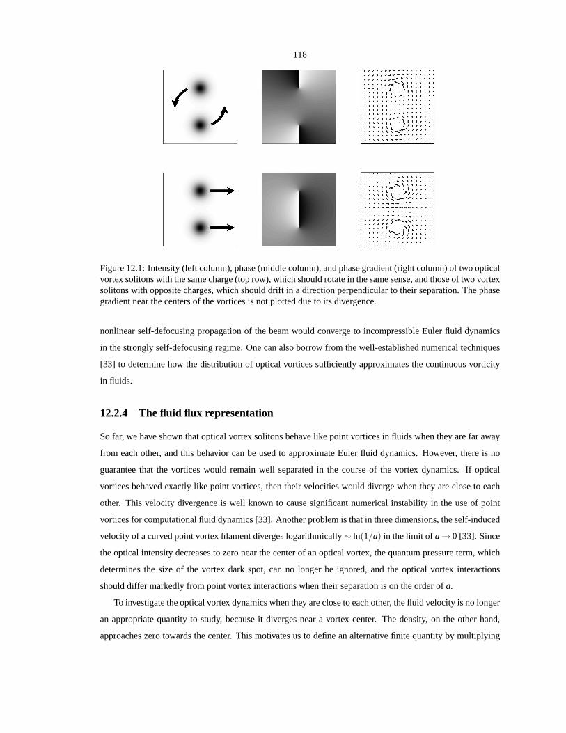
118
Figure 12.1: Intensity (left column), phase (middle column), and phase gradient (right column) of two opticalvortex solitons with the same charge (top row), which shouldrotate in the same sense, and those of two vortexsolitons with opposite charges, which should drift in a direction perpendicular to their separation. The phasegradient near the centers of the vortices is not plotted due to its divergence.
nonlinear self-defocusing propagation of the beam would converge to incompressible Euler fluid dynamics
in the strongly self-defocusing regime. One can also borrowfrom the well-established numerical techniques
[33] to determine how the distribution of optical vortices sufficiently approximates the continuous vorticity
in fluids.
12.2.4 The fluid flux representation
So far, we have shown that optical vortex solitons behave like point vortices in fluids when they are far away
from each other, and this behavior can be used to approximateEuler fluid dynamics. However, there is no
guarantee that the vortices would remain well separated in the course of the vortex dynamics. If optical
vortices behaved exactly like point vortices, then their velocities would diverge when they are close to each
other. This velocity divergence is well known to cause significant numerical instability in the use of point
vortices for computational fluid dynamics [33]. Another problem is that in three dimensions, the self-induced
velocity of a curved point vortex filament diverges logarithmically∼ ln(1/a) in the limit of a → 0 [33]. Since
the optical intensity decreases to zero near the center of anoptical vortex, the quantum pressure term, which
determines the size of the vortex dark spot, can no longer be ignored, and the optical vortex interactions
should differ markedly from point vortex interactions whentheir separation is on the order ofa.
To investigate the optical vortex dynamics when they are close to each other, the fluid velocity is no longer
an appropriate quantity to study, because it diverges near avortex center. The density, on the other hand,
approaches zero towards the center. This motivates us to define an alternative finite quantity by multiplying
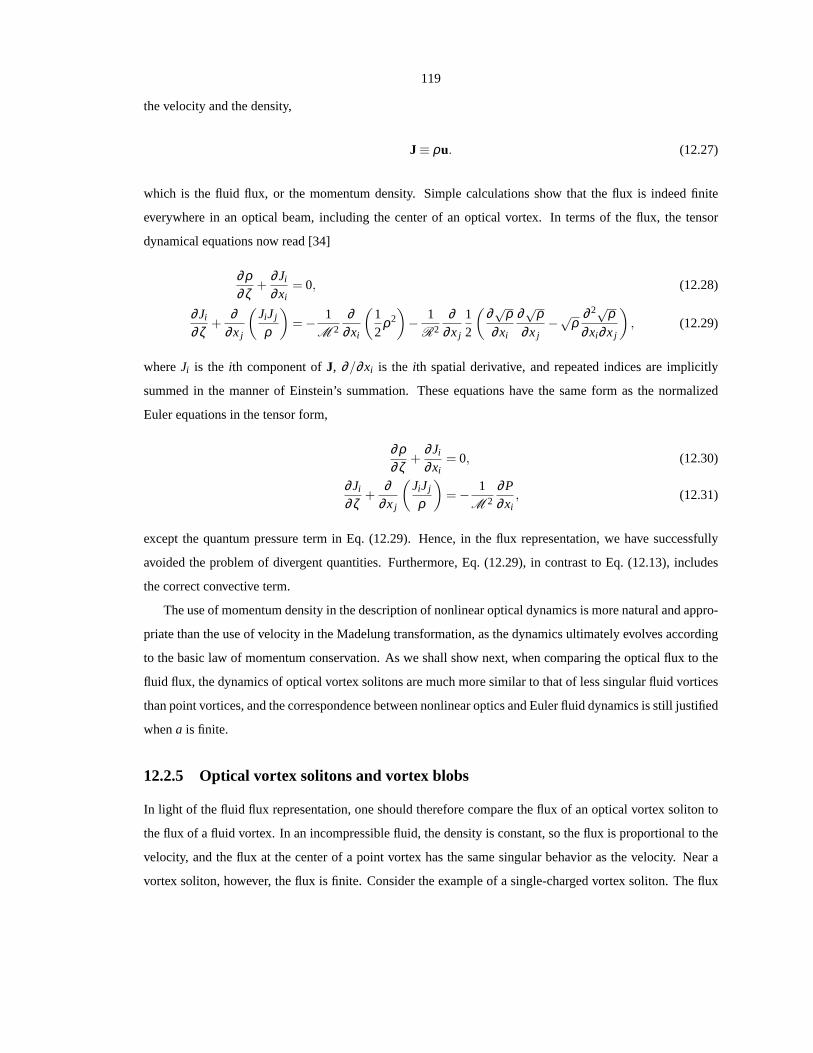
119
the velocity and the density,
J ≡ ρu. (12.27)
which is the fluid flux, or the momentum density. Simple calculations show that the flux is indeed finite
everywhere in an optical beam, including the center of an optical vortex. In terms of the flux, the tensor
dynamical equations now read [34]
∂ρ∂ζ
+∂Ji
∂xi= 0, (12.28)
∂Ji
∂ζ+
∂∂x j
(
JiJ j
ρ
)
= − 1M 2
∂∂xi
(
12
ρ2)
− 1R2
∂∂x j
12
(
∂√ρ∂xi
∂√ρ∂x j
−√ρ
∂ 2√ρ∂xi∂x j
)
, (12.29)
whereJi is the ith component ofJ, ∂/∂xi is the ith spatial derivative, and repeated indices are implicitly
summed in the manner of Einstein’s summation. These equations have the same form as the normalized
Euler equations in the tensor form,
∂ρ∂ζ
+∂Ji
∂xi= 0, (12.30)
∂Ji
∂ζ+
∂∂x j
(
JiJ j
ρ
)
= − 1M 2
∂P∂xi
, (12.31)
except the quantum pressure term in Eq. (12.29). Hence, in the flux representation, we have successfully
avoided the problem of divergent quantities. Furthermore,Eq. (12.29), in contrast to Eq. (12.13), includes
the correct convective term.
The use of momentum density in the description of nonlinear optical dynamics is more natural and appro-
priate than the use of velocity in the Madelung transformation, as the dynamics ultimately evolves according
to the basic law of momentum conservation. As we shall show next, when comparing the optical flux to the
fluid flux, the dynamics of optical vortex solitons are much more similar to that of less singular fluid vortices
than point vortices, and the correspondence between nonlinear optics and Euler fluid dynamics is still justified
whena is finite.
12.2.5 Optical vortex solitons and vortex blobs
In light of the fluid flux representation, one should therefore compare the flux of an optical vortex soliton to
the flux of a fluid vortex. In an incompressible fluid, the density is constant, so the flux is proportional to the
velocity, and the flux at the center of a point vortex has the same singular behavior as the velocity. Near a
vortex soliton, however, the flux is finite. Consider the example of a single-charged vortex soliton. The flux
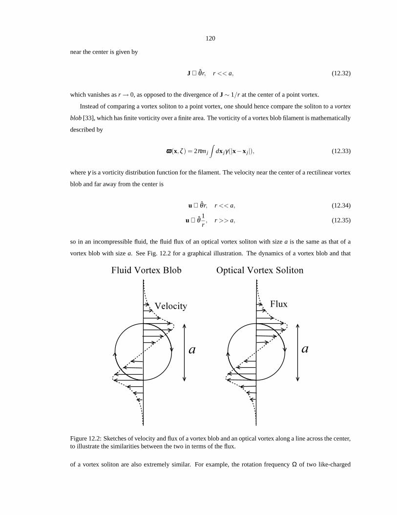
120
near the center is given by
J ∝ θr, r << a, (12.32)
which vanishes asr → 0, as opposed to the divergence ofJ ∼ 1/r at the center of a point vortex.
Instead of comparing a vortex soliton to a point vortex, one should hence compare the soliton to avortex
blob [33], which has finite vorticity over a finite area. The vorticity of a vortex blob filament is mathematically
described by
ωωω(x,ζ ) = 2πm j
∫
dx jγ(|x−x j |), (12.33)
whereγ is a vorticity distribution function for the filament. The velocity near the center of a rectilinear vortex
blob and far away from the center is
u ∝ θr, r << a, (12.34)
u ∝ θ1r, r >> a, (12.35)
so in an incompressible fluid, the fluid flux of an optical vortex soliton with sizea is the same as that of a
vortex blob with sizea. See Fig. 12.2 for a graphical illustration. The dynamics ofa vortex blob and that
Figure 12.2: Sketches of velocity and flux of a vortex blob andan optical vortex along a line across the center,to illustrate the similarities between the two in terms of the flux.
of a vortex soliton are also extremely similar. For example,the rotation frequencyΩ of two like-charged
121
vortex blobs approaches a constant∝ 1/a2 when their separation goes to zero. Numerical simulations of
the nonlinear Schrodinger equation also show that the rotation frequency of two like-charged vortex solitons
approaches a constant∝ 1/a2 and does not diverge like two point vortices [35]. On the other hand, the
self-induced velocity of a curved vortex blob filament is given by [33]
∂xi
∂ζ=
mib2ρc
lnρc
a, (12.36)
whereb is the unit binomial vector of the filament andρc is the radius of curvature. The self-induced velocity
of an optical vortex soliton filament is proven to be exactly the same [29]. Hence, optical vortex solitons
act as vortex blobs, and a large number of solitons can simulate Euler fluid dynamics, much like the popular
discrete vortex blob method in computational fluid dynamics[33].
12.2.6 Numerical evidence of correspondence between nonlinear optics and Euler
fluid dynamics
The most telling evidence of the correspondence between nonlinear optics and Euler fluid dynamics is perhaps
the numerical fluid dynamics simulations using the nonlinear Schrodinger equation by Noreet al. [36, 37].
Using the nonlinear Schrodinger equation, Noreet al. numerically demonstrated the Euler fluid dynamics
of a jet made of an array of counterrotating vortices, which exhibit sinuous and varicose instabilities [36].
In another study, Noreet al. also demonstrated three-dimensional shear flows and showedthat numerically
solving nonlinear Schrodinger equation is a viable alternative to Euler and Navier-Stokes equations for the
numerical study of shear flows [37]. As nonlinear optical propagation is governed by nonlinear Schrodinger
equation, the numerical experiments by Noreet al. show that nonlinear optics should also be able to compute
Euler fluid dynamics.
12.3 Similarities between nonlinear Schrodinger dynamics and Navier-
Stokes fluid dynamics
In the previous sections, we have shown the correspondence between self-defocusing optical propagation
and inviscid Euler fluid dynamics via a variety of methods, including the Madelung transformation, the
incorporation of vorticity effect due to the “phase slip” phenomenon, the fluid flux representation, and the
comparison between optical vortex solitons and vortex blobs. Even though viscosity plays the role of a small
parameter in most interesting fluid dynamics problems, its effects are of paramount importance near a “no-
slip” boundary and in the dissipation of eddies, in which cases the viscous Navier-Stokes equations should
be used. In this section we shall present evidence that the nonlinear Schrodinger equation exhibits many of
the same behaviors of viscous Navier-Stokes fluid dynamics,and in each case, quantum pressure plays an
122
analogous role to viscosity.
The normalized Navier-Stokes equations in the flux representation are given by
∂ρ∂ζ
+∂Ji
∂xi= 0, (12.37)
∂Ji
∂ζ+
∂∂x j
(
JiJ j
ρ
)
= − 1M 2
∂P∂xi
+1R
∂∂x j
(
∂ui
∂x j+
∂u j
∂xi
)
, (12.38)
where the last term in Eq. (12.38) is the viscosity term andR is called the Reynolds number, which describes
the relative strength of convection compared to viscosity,
R =ULν
, (12.39)
whereU is the characteristic velocity of the fluid system,L is the characteristic length, andν is the kine-
matic viscosity of the fluid. Comparing the viscosity term inEq. (12.38) with the quantum pressure term in
Eq. (12.29) via a dimensional analysis would suggest that ananalogous optical Reynolds number would be
defined as
R = KW, (12.40)
where, to recall,K is the characteristic optical phase gradient, andW is the characteristic size of the optical
experiment setup. The optical Reynolds number thus roughlymeasures the number of optical vortices. In
other words, if the optical Reynolds number indeed corresponds to its fluid counterpart, then the quantization
of the optical vortices would play an analogous role to fluid viscosity. This view seems to be echoed by other
researchers in the field of superfluids [38, 39, 40, 41], although we must stress that it is still an open problem
as to what extent the quantization effect resembles the viscous effect [41].
12.3.1 Zero-flux boundary conditions, boundary layers, and boundary layer separa-
tion
In classical fluid dynamics the “no-slip” boundary condition is most commonly used, and restricts the total
velocity and hence the total flux to be zero at the boundary. For fluid flow above a surface, the velocity shear
introduced must be balanced by a viscous stress, resulting in a boundary layer that connects the zero velocity
at the boundary to the flow velocity above the boundary in an asymptotic expansion [42]. For the nonlinear
Schrodinger equation, the boundary condition of an impenetrable object can be specified by a low-refractive-
index region, which restricts the optical intensity to be zero at the surface [43] due to total internal reflection.
Even though the tangential velocity can have a nonzero valueat the surface, both the normal and tangential
components of the flux must be zero there. This can hence be viewed as a zero-flux “no-slip” boundary
condition. An optical boundary layer analogous to the viscous boundary layer in classical fluid dynamics is

123
also formed [43]. See Fig. 12.3 for a graphical illustrationof the similarities between a viscous boundary
layer and an optical boundary layer.
Figure 12.3: Comparison between a viscous boundary layer and an optical boundary layer.
For a viscous fluid flow past an obstacle, as the Reynolds number increases, the boundary layer begins
to separate and vorticity is convected behind the obstacle.An analogy in the dynamics of the nonlinear
Schrodinger equation, in the form of vortex nucleation on the boundary, is also predicted [22], and in the case
of large objects, the instability of the optical boundary layer also depends on the optical Reynolds numberR
defined in Eq. (12.40) [40], much like the viscous boundary layer separation.
12.3.2 Dissipation of eddies
Another important effect of viscosity is the dissipation ofsmall-scale structures in turbulence. An analogous
effect in nonlinear Schrodinger equation is the emission of sound waves two vorticesare close to each other
[35] and the generation of Kelvin waves in the process of vortex line reconnections [44]. The radiation
of acoustic energy in both cases must cause a damping of the high-spatial-frequency convection within the
optical beam, and the effective Reynolds number is again estimated to be equal to the optical Reynolds
number [38, 39, 41].
12.3.3 Karman vortex street
The Karman vortex street is a famous viscous fluid phenomenon, in which alternate fluid vortices are emitted
from the back of an obstacle to the flow of a viscous fluid, when the Reynolds number increases beyond
a certain threshold [26, 45]. Using the numerical vortex blob method, Chorin first simulated such a phe-
nomenon for a cylinder obstacle and obtained good agreementwith experimental data [46]. Since an optical
beam diffracting past a low refractive index region would also emit optical vortices and the vortices inter-
act like vortex blobs in a self-defocusing medium, we performed a numerical experiment of the nonlinear
Schrodinger equation to investigate if we would observe a similar phenomenon for nonlinear optics.
The numerical setup is sketched in Fig. 12.4. A big optical beam is assumed to propagate at an angle
to an ellipsoid cylinder, with a refractive index much lowerthan the surroundings to act as an impenetrable
object, in a self-defocusing medium. The length of the long axis of the ellipsoid cross section is assumed to
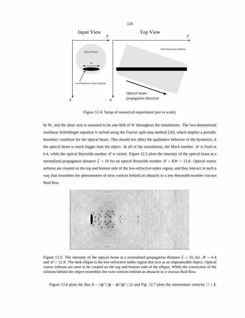
124
Figure 12.4: Setup of numerical experiment (not to scale).
beW , and the short axis is assumed to be one-fifth ofW throughout the simulations. The two-dimensional
nonlinear Schrodinger equation is solved using the Fourier split-step method [20], which implies a periodic
boundary condition for the optical beam. This should not affect the qualitative behavior of the dynamics, if
the optical beam is much bigger than the object. In all of the simulations, the Mach numberM is fixed at
0.4, while the optical Reynolds numberR is varied. Figure 12.5 plots the intensity of the optical beam at a
normalized propagation distanceζ = 10 for an optical Reynolds numberR = KW = 12.8. Optical vortex
solitons are created on the top and bottom side of the low-refractive-index region, and they interact in such a
way that resembles the phenomenon of twin vortices behind anobstacle in a low-Reynolds-number viscous
fluid flow.
Figure 12.5: The intensity of the optical beam at a normalized propagation distanceζ = 10, for M = 0.4andR = 12.8. The dark ellipse is the low-refractive-index region thatacts as an impenetrable object. Opticalvortex solitons are seen to be created on the top and bottom side of the ellipse, While the convection of thesolitons behind the object resembles the twin vortices behind an obstacle in a viscous fluid flow.
Figure 12.6 plots the fluxJ = (ψ∗∇ψ −ψ∇ψ∗)/2i and Fig. 12.7 plots the momentum vorticity∇× J.

125
Both plots confirm the similarity between the numerically observed dynamics and the phenomenon of twin
vortices in a viscous fluid flow.
Figure 12.6: A vector plot of the fluxJ at ζ = 10, forM = 0.4 andR = 12.8, which confirms the similaritybetween the numerically observed dynamics and the phenomenon of twin vortices.
Figure 12.7: A plot of the momentum vorticity∇× J at ζ = 10, for M = 0.4 andR = 12.8. A white dotindicates that the vortex has a positive topological chargeand a black dot indicates that the vortex has a neg-ative charge. The plot shows the similarity between the numerically observed dynamics and the phenomenonof twin vortices.
Figures 12.8, 12.9, and 12.10 plot the intensity, flux, and momentum vorticity of the optical beam respec-
tively, at a longer propagation distanceζ = 20 for the same parameters. The qualitative dynamical behavior
of vortices staying behind the object is essentially unchanged.
We now raise the Reynolds number toR = 25.6 and perform the numerical experiment again. As seen
from Figs. 12.11, 12.12, and 12.13, the optical vortex solitons become smaller and more abundant, but at
ζ = 10 the phenomenon of twin vortices behind an obstacle is again observed.
At ζ = 20, however, significant instability in the twin vortices develops, such that the spatial symmetry
between the upper plane and the lower plane is broken, and alternative bunches of optical vortices begin to
be emitted from the back of the object. Figures 12.14, 12.15,and 12.16 plot the intensity, flux and vorticity

126
Figure 12.8: The intensity of the optical beam at a normalized propagation distanceζ = 20, forM = 0.4 andR = 12.8. The qualitative dynamical behavior is essentially unchanged from that shown in Fig. 12.5.
Figure 12.9: A vector plot of the fluxJ at ζ = 20, forM = 0.4 andR = 12.8.
Figure 12.10: A plot of the momentum vorticity∇×J at ζ = 20, forM = 0.4 andR = 12.8.

127
Figure 12.11: The optical intensity atζ = 10, forM = 0.4 andR = 25.6. The vortex solitons are observedto be smaller, and the phenomenon of twin vortices is again observed.
Figure 12.12: The fluxJ at ζ = 10, forM = 0.4 andR = 25.6.
Figure 12.13: The momentum vorticity∇×J at ζ = 10, forM = 0.4 andR = 25.6.

128
at ζ = 20 respectively, which demonstrate a behavior strongly resembling the famous Karman vortex street
phenomenon.
Figure 12.14: Optical intensity atζ = 20, for M = 0.4 andR = 25.6. The twin vortices become unstableand detach alternatively from the object.
Figure 12.15: Flux atζ = 20, forM = 0.4 andR = 25.6, which shows a flow pattern strongly resemblingthe Karman vortex street.
Due to computing power constraints, we are only able to simulate low-Reynolds-number flows, which
we do not expect to quantitatively reproduce viscous fluid dynamics. We have to use an ellipsoid cylinder in
the numerical experiments, instead of the more conventional circular cylinder, to artificially generate more
optical vortices, and the Mach number is a little too high forcompressional waves not to play a significant role
in the dynamics. With all that said, using the nonlinear Schrodinger equation, we are still able to qualitatively
demonstrate, for the first time to our knowledge, two well-known viscous fluid phenomena, namely, the
formation of twin vortices behind an obstacle, and the symmetry-breaking instability of the twin vortices that
leads to the Karman vortex street when the Reynolds number is increased. Compared with previous claims of
observing the Karman vortex street in nonlinear optics numerically [7] or experimentally [8, 9], our numerical
results demonstrate an unprecedented level of correspondence between nonlinear optical dynamics and the
Karman vortex street phenomenon, thanks to the presence of a muchlarger number of optical vortices in our
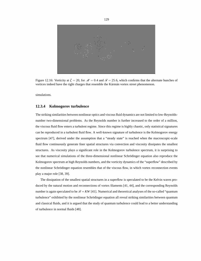
129
Figure 12.16: Vorticity atζ = 20, forM = 0.4 andR = 25.6, which confirms that the alternate bunches ofvortices indeed have the right charges that resemble the Karman vortex street phenomenon.
simulations.
12.3.4 Kolmogorov turbulence
The striking similarities between nonlinear optics and viscous fluid dynamics are not limited to low-Reynolds-
number two-dimensional problems. As the Reynolds number isfurther increased to the order of a million,
the viscous fluid flow enters a turbulent regime. Since this regime is highly chaotic, only statistical signatures
can be reproduced in a turbulent fluid flow. A well-known signature of turbulence is the Kolmogorov energy
spectrum [47], derived under the assumption that a “steady state” is reached when the macroscopic-scale
fluid flow continuously generate finer spatial structures viaconvection and viscosity dissipates the smallest
structures. As viscosity plays a significant role in the Kolmogorov turbulence spectrum, it is surprising to
see that numerical simulations of the three-dimensional nonlinear Schrodinger equation also reproduce the
Kolmogorov spectrum at high Reynolds numbers, and the vorticity dynamics of the “superflow” described by
the nonlinear Schrodinger equation resembles that of the viscous flow, in whichvortex reconnection events
play a major role [38, 39].
The dissipation of the smallest spatial structures in a superflow is speculated to be the Kelvin waves pro-
duced by the natural motion and reconnections of vortex filaments [41, 44], and the corresponding Reynolds
number is again speculated to beR = KW [41]. Numerical and theoretical analyses of the so-called “quantum
turbulence” exhibited by the nonlinear Schrodinger equation all reveal striking similarities betweenquantum
and classical fluids, and it is argued that the study of quantum turbulence could lead to a better understanding
of turbulence in normal fluids [48].
130
12.4 The split-step method
While a nonlinear optical system shows promise for computingEuler and Navier-Stokes fluid dynamics, it
also poses serious technical challenges. Ideally one wouldlike to have a configurable nonlinear material
with low loss, anomalous group-velocity dispersion, high defocusing nonlinearity, and three-dimensional
copropagating boundaries. One may only be able to find separate materials or optical devices, each of which
performs only some of the functions. Moreover, parasitic effects such as loss, two-photon absorption, and
high-order dispersion can be detrimental to the accuracy. To combine different devices and periodically
compensate for parasitic effects, we hereby propose the “split-step” method, the inspiration of which comes
from the numerical Fourier “split-step” method [20]. Consider the general nonlinear Schrodinger equation
∂ψ∂ζ
=N
∑n=1
Hnψ, (12.41)
where propagation effects and boundary conditions are expressed in terms of operatorsHn. The formal
solution is
ψ(ζ +∆ζ ) = exp(
∫ ζ+∆ζ
ζ
N
∑n=1
Hndζ ′)
ψ(ζ ). (12.42)
But if ∆ζ is much smaller than 1/H whereH is the magnitude of the operators, by virtue of the Baker-
Hausdorff formula we have
ψ(ζ +∆ζ ) =N
∏n=1
exp(
Hn∆ζ)
ψ(ζ )+O(H2∆ζ 2). (12.43)
Each of the propagation effects can hence be applied separately to an optical pulse, with a quadratic error
term. A symmetrized version of the split-step method can further reduce the error order,
ψ(ζ +∆ζ ) =1
∏m=N
exp(
Hm∆ζ2
) N
∏n=1
exp(
Hn∆ζ2
)
ψ(ζ )+O(H3∆ζ 3). (12.44)
The split-step method is not unlike the proof of a quantum computer being able to simulate any quantum
systems [23]. Whereas it is difficult to find a quantum device that performs the exact Hamiltonian of the
quantum system of interest, it is possible to approximate the Hamiltonian in small time slices. Similarly, in a
metaphoric optical computer, one can form a unit cell of a “meta-material” by combining a slice of defocusing
material, a slice of material with anomalous group-velocity dispersion, a slice of ultrafast phase modulator
to apply the three-dimensional boundary conditions, and a gain medium to compensate for loss. The optical
beam can loop through the unit cell multiple times in a cavity, so that the outcome will approximate the true
solution as if we had an ideal medium. See Fig. 12.17 for a graphical illustration of the method.
The split-step method has the additional advantages that each subsystem can be tunable and easily substi-
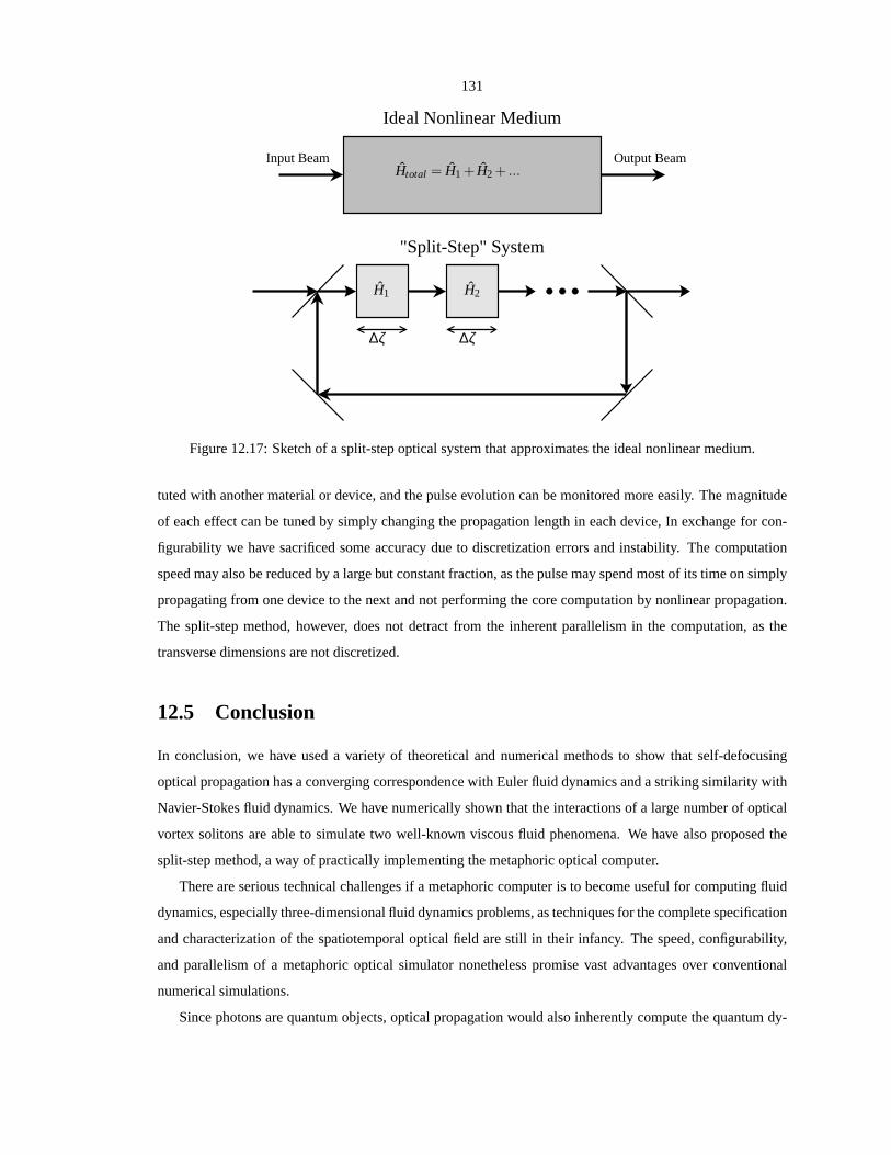
131
Input Beam Output Beam
Ideal Nonlinear Medium
"Split-Step" System
Htotal = H1 + H2 + ...
H1 H2
∆ζ∆ζ
Figure 12.17: Sketch of a split-step optical system that approximates the ideal nonlinear medium.
tuted with another material or device, and the pulse evolution can be monitored more easily. The magnitude
of each effect can be tuned by simply changing the propagation length in each device, In exchange for con-
figurability we have sacrificed some accuracy due to discretization errors and instability. The computation
speed may also be reduced by a large but constant fraction, asthe pulse may spend most of its time on simply
propagating from one device to the next and not performing the core computation by nonlinear propagation.
The split-step method, however, does not detract from the inherent parallelism in the computation, as the
transverse dimensions are not discretized.
12.5 Conclusion
In conclusion, we have used a variety of theoretical and numerical methods to show that self-defocusing
optical propagation has a converging correspondence with Euler fluid dynamics and a striking similarity with
Navier-Stokes fluid dynamics. We have numerically shown that the interactions of a large number of optical
vortex solitons are able to simulate two well-known viscousfluid phenomena. We have also proposed the
split-step method, a way of practically implementing the metaphoric optical computer.
There are serious technical challenges if a metaphoric computer is to become useful for computing fluid
dynamics, especially three-dimensional fluid dynamics problems, as techniques for the complete specification
and characterization of the spatiotemporal optical field are still in their infancy. The speed, configurability,
and parallelism of a metaphoric optical simulator nonetheless promise vast advantages over conventional
numerical simulations.
Since photons are quantum objects, optical propagation would also inherently compute the quantum dy-

132
namics of bosons, and may therefore be used as a metaphoric simulator of quantum fluids, such as superfluids,
superconductors, and Bose-Einstein condensates. In this way the advantages of a metaphoric computer and
those of a quantum computer are combined, and only then the classical and quantum computing capabili-
ties offered by photons would truly be exhausted. This extension of metaphoric optical computing will be a
subject of future work.
133
Bibliography
[1] W. G. Wagner, H. A. Haus, and J. H. Marburger, Phys. Rev.175, 256 (1968).
[2] P. Coullet, L. Gil, and F. Rocca, Opt. Commun.73, 403 (1989).
[3] M. Brambilla, L. A. Lugiato, V. Penna, F. Prati, C. Tamm, and C. O. Weiss, Phys. Rev. A43, 5114 (1991).
[4] F. T. Arecchi, G. Giacomelli, P. L. Ramazza, and S. Residori, Phys. Rev. Lett.67, 3749 (1991).
[5] S. A. Akhmanov, M. A. Vorontsov, V. Yu. Ivanov, A. V. Larichev, and N. I. Zheleznykh, J. Opt. Soc. Am.
B 9, 78 (1992).
[6] G. A. Swartzlander, Jr. and C. T. Law, Phys. Rev. Lett.69, 2503 (1992).
[7] K. Staliunas, Phys. Rev. A48, 1573 (1993).
[8] M. Vaupel, K. Staliunas, and C. O. Weiss, Phys. Rev. A54, 880 (1996).
[9] G. Molina-Terriza, D. V. Petrov, J. Recolons, and L. Torner, Opt. Lett.27, 625 (2002).
[10] F. S. Roux, J. Opt. Soc. Am. B12, 1215 (1995).
[11] D. Rozas, C. T. Law, and G. A. Swartzlander, Jr., J. Opt. Soc. Am. B14, 3054 (1997).
[12] D. Rozas, Z. S. Sacks, and G. A. Swartzlander, Jr., Phys.Rev. Lett.79, 3399 (1997).
[13] H. Michinel, J. Campos-Taboas, R. Garcıa-Fernandez, J. R. Salgueiro, and M. L. Quiroga-Teixeiro,
Phys. Rev. E65, 066604 (2002).
[14] M. J. Paz-Alonso, D. Olivieri, H. Michinel, and J. R. Salgueiro, Phys. Rev. E69, 056601 (2004).
[15] M. J. Paz-Alonso and H. Michinel, Phys. Rev. Lett.94, 093901 (2005).
[16] Y. Pomeau and S. Rica, C. R. Acad. Sci. Paris,317, 1287 (1993).
[17] E. L. Bolda, R. Y. Chiao, and W. H. Zurek, Phys. Rev. Lett.86, 416 (2001).
[18] R. Y. Chiao, Opt. Commun.179157 (2000).
[19] R. W. Boyd,Nonlinear Optics (Academic Press, San Diego, 2002).

134
[20] G. P. Agrawal,Nonlinear Fiber Optics (Academic Press, San Diego, 2001).
[21] R. J. Donnelly,Quantized Vortices in Helium II (Cambridge University Press, New York, 1991).
[22] T. Frisch, Y. Pomeau, and S. Rica, Phys. Rev. Lett.69, 1644 (1992).
[23] S. Lloyd, Science273, 1073 (1996).
[24] E. Madelung, Z. Phys.40, 322 (1926).
[25] M. Quiroga-Teixeiro and H. Michinel, J. Opt. Soc. Am. B14, 2004 (1997).
[26] L. M. Milne-Thomson,Theoretical Hydrodynamics (The Macmillan Company, New York, 1968).
[27] A. W. Snyder, L. Poladian, and D. J. Mitchell, Opt. Lett.17789 (1992).
[28] J. C. Neu, Physica D43, 407 (1990).
[29] L. M. Pismen and J. Rubinstein, Physica D47, 353 (1991).
[30] F.-H. Lin and J. X. Xin, Commun. Math. Phys.200, 249 (1999).
[31] T.-C. Lin, SIAM J. Appl. Math.60, 1099 (2000).
[32] E. B. Sonin, Rev. Mod. Phys.59, 87 (1987).
[33] A. Leonard, J. Comp. Phys.37, 289 (1980).
[34] J. Grant, J. Phys. A6, L151 (1973).
[35] I. Aranson and V. Steinberg, Phys. Rev. B53, 75 (1996).
[36] C. Nore, M. E. Brachet, and S. Fauve, Physica D65, 154 (1993).
[37] C. Nore, M. Abid, and M. E. Brachet, C. R. Acad. Sci. Paris, 319, 733 (1994).
[38] C. Nore, M. Abid, and M. E. Brachet, Phys. Rev. Lett.78, 3896 (1997).
[39] C. Nore, M. Abid, and M. E. Brachet, Phys. FLuids9, 2644 (1997).
[40] J. S. Stiessberger and W. Zwerger, Phys. Rev. A62, 061601 (2000).
[41] W. F. Vinen and J. J. Niemela, J. Low Temp. Phys.128, 167 (2002).
[42] H. Schlichting, K. Gersten, E. Krause, and H. Oertel Jr., Boundary-Layer Theory (Springer, New York,
2000).
[43] N. G. Berloff and P. H. Roberts, J. Phys. A33, 4025 (2000).
[44] E. Kozik and B. Svistunov, Phys. Rev. Lett.92, 035301 (2004).
135
[45] C. H. K. Williamson, Annu. Rev. Fluid. Mech.28,477 (1996).
[46] A. J. Chorin, J. Fluid Mech.57, 785 (1973).
[47] U. Frisch,Turbulence, the Legacy of A. N. Kolmogorov (Cambridge University Press, Cambridge, 1995).
[48] S. N. Fisher and G. R. Pickett, “Quantum turbulence,” Phys. World April Issue (2006).


