
, i, .6I
Brookhaven National Laboratory Report
BNL-NUREG-35597 (1984)
submitted to CORROSION
Potential--pH Diagrams and Solubility Limits of Ti, Cu and Pb for
Simulated Rock Salt Brines at 250C and 1000C
T. M. Ahn and S. Aronson*Department of Nuclear EnergyBrookhaven National Laboratory
Upton, Few York 11973
KEY WORDS: Potential--pH Diagrams, Solubility Limit, Ti, Cu, Pb
*Address: Brooklyn College, Brooklyn, New York 11210
1
-a,./ ~? Cx * .-

ABSTRACT
Titanium, lead and copper have been considered as candidate materials for
high level nuclear waste containers in rock salt repositories. The thermo-
dynamic properties are characterized for the systems of Ti, Cu and Pb in simu-
lated rock salt brines at 250C and 1000C. The potential--pH diagram of Ti
in the brines is close to that for pure water, and, in neutral solutions,
stable oxides are present and Ti dissolution is not significant. In acidic
environments at low potential, however, titanium dissolves in ionic forms.
Such cases include crevice or pitting corrosion. For copper, new domains of
copper chloride or copper sulfate compounds are introduced into the potential
--pH diagram for pure water. The dissolution of copper chlorocomplexes re-
sults in a significant metal loss by uniform corrosion. Lead chloride domains
are also introduced and this compound is considered to affect the uniform cor-
rosion of lead. However, metal loss by chlorocomplexes is not observed for
lead. The implications of the calculated results are discussed for both
uniform and local corrosion processes.
2
T L
FIGURES
1. Potential-pH equilibrium diagram for the titanium-brine system
at 25 0C . . . . . a * * * * * * * * * * * * * * * * a * * * * * * * * * 14
2. Potential-pH equilibrium diagram for the titanium-brine system
at 1000C.. . . . . . . . . . .
3. Log [ratio of titanium compound activity a~z to titai
for brine A at 25C . . . . . ..........
4. Log [ratio of titanium compound activity a~y to titam
for brine A at 100C . . . . . . .........
5. Log [ratio of titanium compound activity aXy to titai
for brine B at 25C .. .............
6. Log [ratio of titanium compound activity a y to titai
for brine B at 100C ................
7. Potential-pH equilibrium diagram for the copper-brine
at 25°C .......................0 * & 0
...i .. activity a 15
nium activity aTil
** 0 0 0 * * .. * 17
Aium activity aTi]
..... .............. 17
anium activity aTi]
18* *C C C * * C C
Aium activity aTi]
C & C C * C C
sys ten
* * . . . . C
. 19
. . 20
8. Potential-pH equilibrium diagram for the copper-brine system
at 1000C .............................. * & 0 a 0
9. Log [ratio of copper compound activity aXY to copper activity aCu]
for brine A at 25C . . . . . . . . . . . . . . . . . . . . . .
10. Log ratio of copper compound activity a/,y to copper activity aCul
for brine B at 25 0C . . . . . . . . . . . . . . . . . . . . . . .
11. Log [ratio of copper compound activity aXy to copper activity aCul
for brine A at 100'C .. . .. ... . . * C C C C . .*
. 21
. . 22
. . 23
. . 24
3

t
I I I ;
12. Log [ratio of copper compound activity a y to copper activity aCu]
for brine B at 1000C . . . . . . . . . . . . . . . . . . . . ...
13. Potential-pH equilibrium diagram for the lead-brine system
at 25°C . . . . . . . . . . . . . . .
14. Potential-pH equilibrium diagram for the lead-brine system
at 1000C .. .. . . . . . . .................. * . * * * * *
15. Log [ratio of lead compound activity a Y to lead activity apb]
for brine A at 25°C . . . . . .............
16. Log [ratio of lead compound activity ap4,Xy to lead activity apb]
for brine B at 25*C . . . . . . . . . . . . . . . . . . . . . .
17. Log [ratio of lead compound activity apx to lead activity aI
* a 25
, . 26
, a 27
. 28
. 29
for brine A at 100C . a. ........... * * . .... * . *. .
I8. Log [ratio of lead compound activity ak- y to lead activity ab]
for brine B at 100%C . .. . . *. . . . . . * . . * *.
* . 30
. . . 31
4

I
TABLES
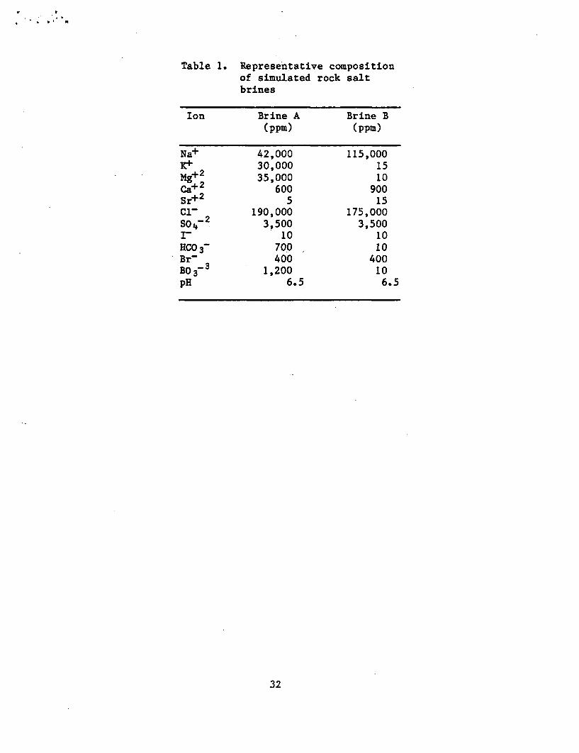
1. Representative composition of simulated rock salt brines . . . . . . . . . 32
2. Activites (moles/liter) used in the calculations . . . . . . . . . . . . . 33
3. Reactions used in the calculations for the titanium-brine system . . . . . 34
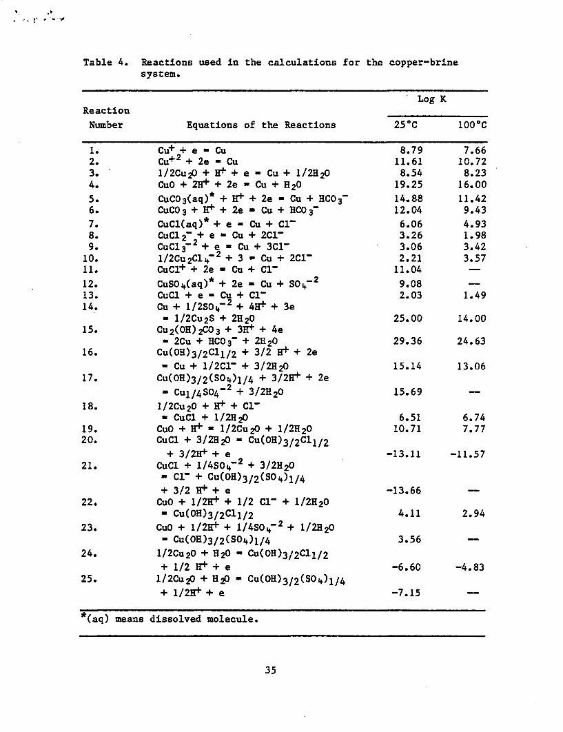
4. Reactions used in the calculations for the copper-brine system . . . . . . 35
5. Reactions used in the calculations for the lead-brine system . . . . . . . 36
5

-
I b I I
ACKNOWLEDGMENTS
This work was supported by the Nuclear Regulatory Commission (RC) andthe program was coordinated by Dr. M. MeNeil of the NRC. The authorsacknowledge Dr. E. D. Verink, Jr. of University of Florida for his helpfulsuggestions in the beginning of this work.
6

t
1. INTRODUCTION
One of the major criteria for high level nuclear waste storage is the
containment of radioactive ions 300 to 1000 years.(l) Metal containers are
expected to be the waste package components that will be used to meet this
criterion. Rock salt is a potential repository host rock and titanium and
titanium base alloys(2) are candidates for the container material because of
their corrosion resistance in high chloride environments formed in rock salt
brine pockets. Copper(3) is also considered because of its noble character-
istics and simple microstructure. Lead is used to shield radiation fields
from the waste.(4) Thermodynamic characterization of these systems is
essential to understand the corrosion properties of these materials in
hig-chloride waters.
The usefulness of potential--pH diagram is widely recognized for the
study of corrosion, along with solubility limit diagrams. Although pure
metal-water systems have been well studied and tabulated(5) at room tempera-
ture, high temperature data for the present systems are not available. This
paper presents potential--pH diagrams and solubility limit diagrams for
titanium, copper and lead in simulated rock salt brines at room temperature
and 1000C.
2. CALCULATION PROCEDURES
Table 1 shows the compositions of simulated rock salt brines.(6) In
the calculations, C, S04-2, I-1, HC03 - and H1I are considered
to be the most detrimental ions with respect to corrosion. The compounds
formed from these ions are potentially stable. However, HCO3- and I-
7
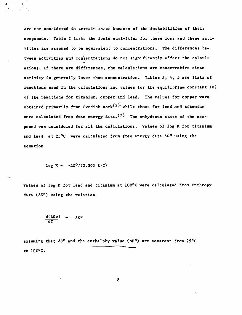
are not considered in certain cases because of the instabilities of their
compounds. Table 2 lists the ionic activities for these ions and these acti-
vities are assumed to be equivalent to concentrations. The differences be-
tween activities and consentrations do not significantly affect the calcul-
ations. If there are differences, the calculations are conservative since
activity is generally lower than concentration. Tables 3, 4, 5 are lists of
reactions used in the calculations and values for the equilibrium constant (K)
of the reactions for titanium, copper and lead. The values for copper were
obtained primarily from Swedish work(3> while those for lead and titanium
were calculated from free energy data.(7) The anhydrous state of the com-
pound was considered for all the calculations. Values of log K for titanium
and lead at 250C were calculated from free energy data AGO using the
equa tion
log K - -AGO/(2.303 RT)
Values of log K for lead and titanium at 1000C were calculated from enthropy
data (ASO) using the relation
d(AGo) , _ ASo
dT
assuming that AS0 and the enthalphy value (AHO) are constant from 250C
to 1000C.
8
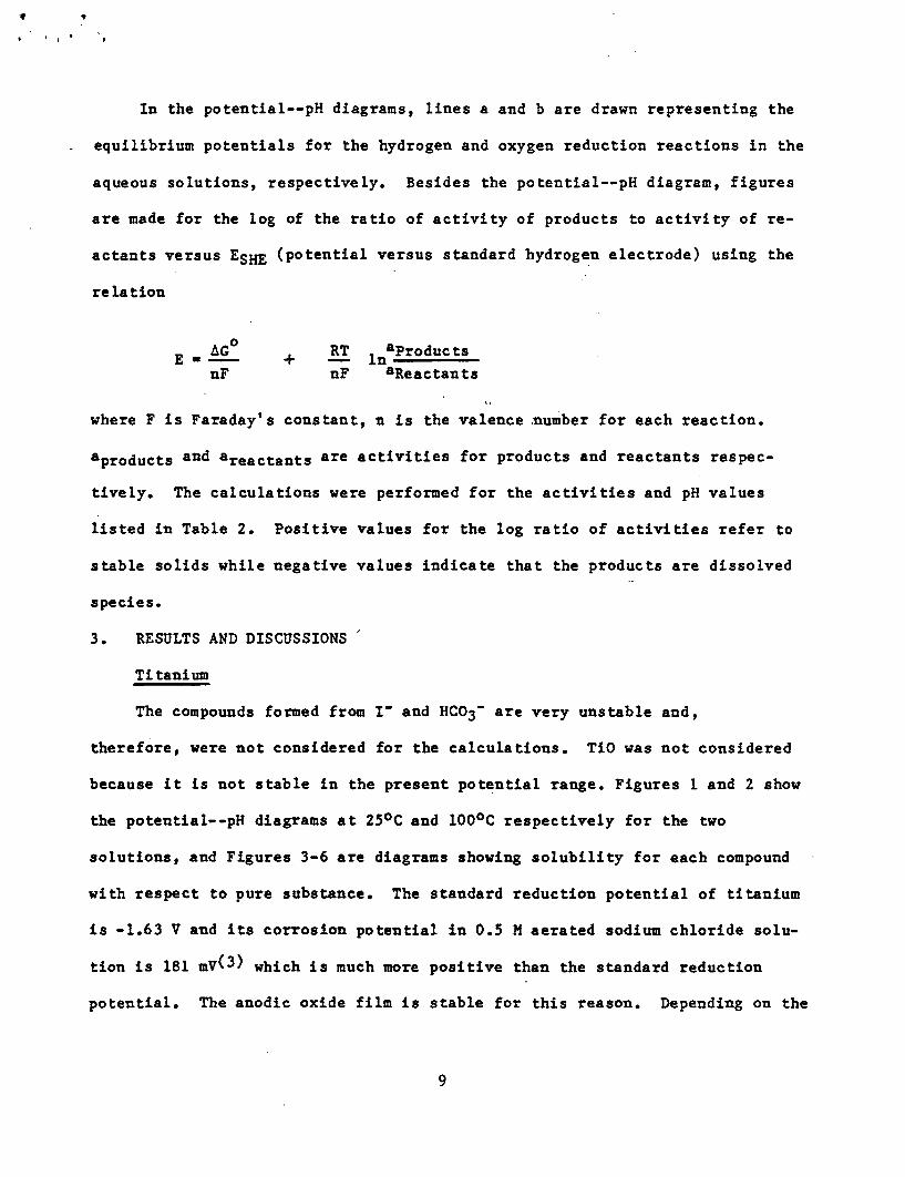
In the potential--pH diagrams, lines a and b are drawn representing the
equilibrium potentials for the hydrogen and oxygen reduction reactions in the
aqueous solutions, respectively. Besides the potential--pH diagram, figures
are made for the log of the ratio of activity of products to activity of re-
actants versus ESHF (potential versus standard hydrogen electrode) using the
relation
AG0 RT aProductsEm + - innF nF aReactants
where F is Faraday's constant, n is the valence number for each reaction.
aproducts and areactants are activities for products and reactants respec-
tively. The calculations were performed for the activities and pH values
listed in Table 2. Positive values for the log ratio of activities refer to
stable solids while negative values indicate that the products are dissolved
species.
3. RESULTS AND DISCUSSIONS
Titanium
The compounds formed from I and HCO3- are very unstable and,
therefore, were not considered for the calculations. TiO was not considered
because it is not stable in the present potential range. Figures 1 and 2 show
the potential--pH diagrams at 250C and 1000C respectively for the two
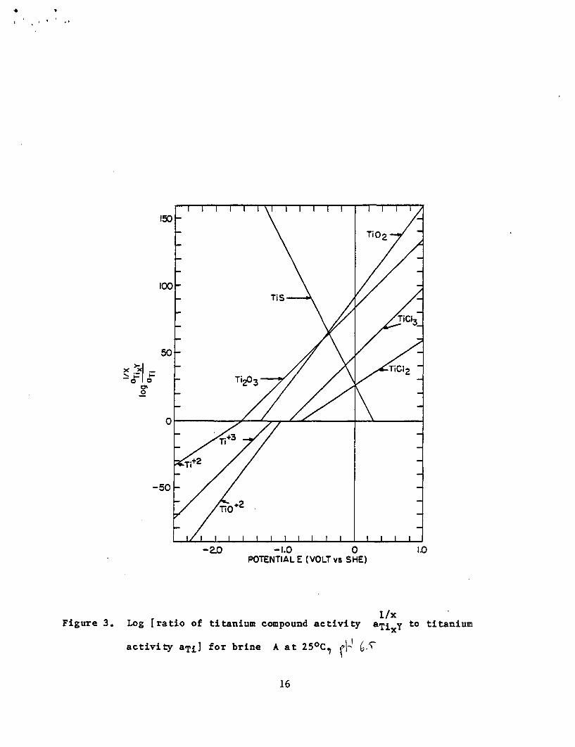
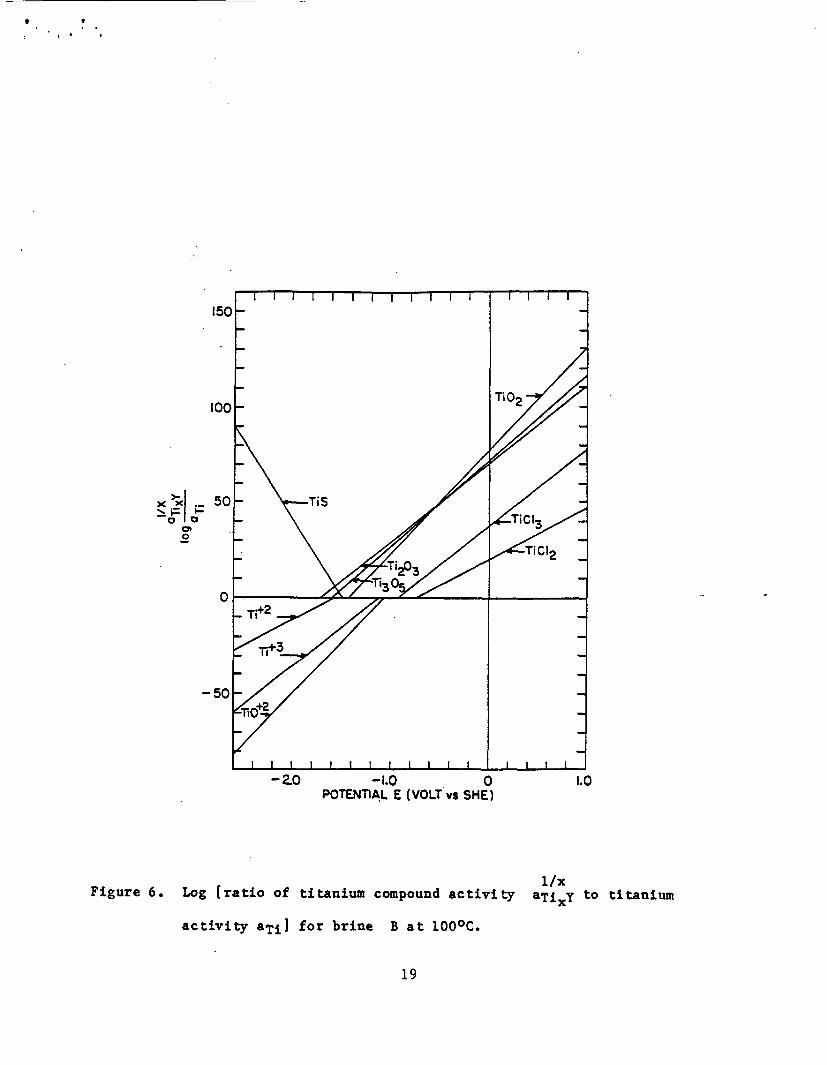
solutions, and Figures 3-6 are diagrams showing solubility for each compound
with respect to pure substance. The standard reduction potential of titanium
is -1.63 V and its corrosion potential in 0.5 M aerated sodium chloride solu-
tion is 181 mV(3) which is much more positive than the standard reduction
potential. The anodic oxide film is stable for this reason. Depending on the
9

V T
degree of aeration, the corrosion potential is probably in the range of 0 to
200 mV. Therefore, the present potential--pH diagrams indicate that a stable
passivating film should be present in all cases. In the range of our pH
values, the concentration of dissolved titanium species will be negligible and
there are no stable chlorocomplexes of titanium. However, when the environ-
ments are occluded, crevice or pit solutions will be formed. The crevice and
pit solutions are typically acidic and deaerated.(8) Figures 3-6 show the
possibilities of high dissolution of Ti+2, Ti+3 ad TiO+2 for such
cases. It is observed in the above mentioned figures that solid titanium
chlorides are much less stable than the titanium oxides. Therefore, the
chloride compounds should not be present as stable compounds and high chloride
content should not affect the uniform corrosion behavior of titanium.
Copper
The compounds formed from I- are not very stable and, therefore, were
not be considered. Figures 7-8 show the potential--pH diagrams at 250C and
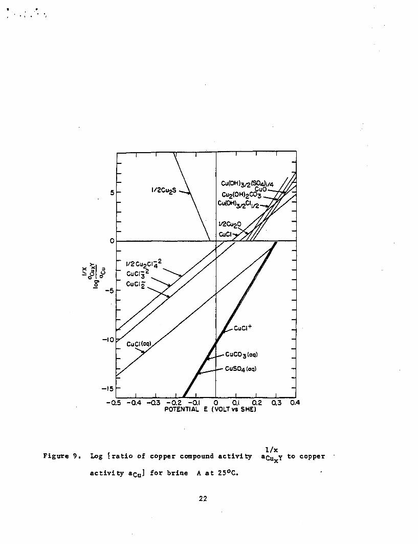
1000C, respectively, for the brines and Figures 9-12 are diagrams showing
solubility for each compound with respect to pure substance. The standard
reduction potential of copper is +337 mV and its corrosion potential in 0.5 M
aerated sodium chloride solution is reportd to be +58 mV.(9) Depending on
the degree of aeration of the solutions, the corrosion potential of copper
should range between -200 mV and +50 mV. If the potential is positive, the
solid phases Cu20, CuO, Cu(OH)3 /2Cll/2 or Cu(OH)1 /2(SO4)1/4 or
Cu(OH)4 /3 (S04)1/3] and or CuCl will form depending on the temperature
and the composition of the solution. Other stable phases are those observed
in the system Cu-water.(5) Another effect of the high chloride content is
the high solubility of copper in the form of chlorocomplexes (Figures 9-12).
10

If the potential is between 0 and -200 m, dissolution of copper to form
aqueous copper chlorocompelxes is very high based on a simple mass balance
calculation of the dissolved ions using a diffusivity 10-5 cm2/sec(l0)
for the copper complexes in water.
The concentrations of S04-2 and HC03- are significant in the pre-
sent solutions. The compounds Cu(OH)3/2 (S04)1 /4 and
Cu(OH)4 /3(S04)1 /3 are only slightly less stable than Cu(OH)3/2 C 11/2.
These phases as well as Cu(OH)(C03)1/2 may, therefore, play a role in
corrosion and appear as corrosion products.
The line referring to the formation of metal sulfide is the only cathodic
corrosion reaction shown in Figures 9-12 where a negative slope is shown for
metal sulfide. In the cathodic corrosion, sulfate ions are reduced to sulfide
ions in reacting with the metal. These reaction may be kinetically slow and,
hence, do not seem to significantly affect the corrosion.(3) It is also
noted that the interaction of ions other than those in Table 2 has not been
considered in producing the Potential--pH diagrams. In particular, the pro-
posed g+2 content in brines is 1.5M. At high pH values (above 8.5), solid
Mg(OH)2 and possibly gCO3 should form. Their presence could also have
some indirect effects on the corrosion.
Lead
The stability of PbSO4 (or PbC12, or PbCO3) are highlighted in the
potential--pH diagram as shown in Figures 13-14 compared to its absence in the
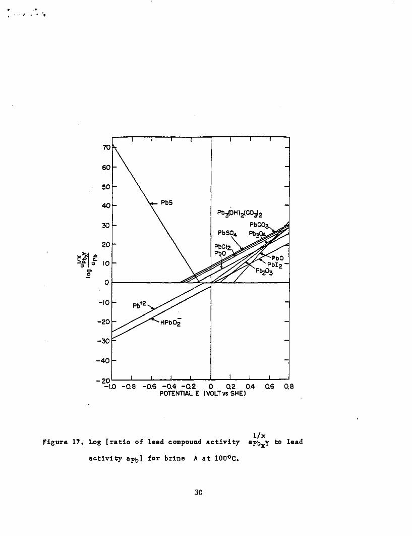
lead-water system.(5) Figures 15-18 are diagrams showing solubility for
each compound with respect to pure substance. The standard reduction poten-
tial of lead is -126 mV and its corrosion potential in 0.5M aerated sodium
11

chloride solution is -312 mV.(9) Depending on the degree of aeration of the
solutions, the corrosion potential may range from -500 mV to -300 mV. Dis-
solution of lead into soluble species may not be a major problem at these
potentials and temperatures of 250C and 1000C as shown in Figures 15-18.
At temperatures above 1000C and at pH above 8, the concentration of aqueous
HPbO2- could become sufficiently large to cause a possibly significant
dissolution of lead. No solid compounds of lead are formed at potentials more
negative than -300 mV. Data in these figures show that lead might be stable
if the oxygen content of the aqueous environment is low, resulting in a more
negative ESHE value and if the pH remains between 6.5 and 8.1. The primary
effects of high chloride content are the formation of solid PbC12 since
stable aqueous hlorocomplexes of lead do not occur. The formation of this
compound may affect the passivity of any solid film formed on the metal.
4. CONCLUSIONS
The thermodynamic properties have been characterized for the systems of
Ti, Cu and Pb in simulated rock salt brines at 250C and 1000C. For
titanium, no new domain has been introduced in the potential -pH diagram and
metal dissolution is not significant. For copper, new domains of copper
chloride or copper sulfate compounds have been introduced. The dissolution of
copper chlorocomplexes are the source of significant metal loss. Lead sulfate
domains are introduced in the lead potential -pH diagrams. Metal loss by
chlorocomplex formation of lead has not been found. Effects of other minor
ions are discussed.
12
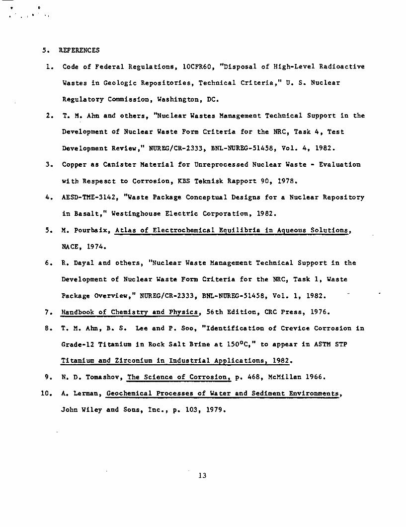
5. REFERENCES
1. Code of Federal Regulations, 10CFR60, "Disposal of High-Level Radioactive
Wastes in Geologic Repositories, Technical Criteria," U. S. Nuclear
Regulatory Commission, Washington, DC.
2. T. M. Ahn and others, "Nuclear Wastes Management Technical Support in the
Development of Nuclear Waste Form Criteria for the NRC, Task 4, Test
Development Review," NUREG/CR-2333, BNL-NUREG-51458, Vol. 4, 1982.
3. Copper as Canister Material for Unreprocessed Nuclear Waste - Evaluation
with Respesct to Corrosion, KBS Teknisk Rapport 90, 1978.
4. AESD-TME-3142, "Waste Package Conceptual Designs for a Nuclear Repository
in Basalt," Westinghouse Electric Corporation, 1982.
5. M. Pourbaix, Atlas of Electrochemical Equilibria in Aqueous Solutions,
NACE, 1974.
6. R. Dayal and others, "Nuclear Waste Management Technical Support in the
Development of Nuclear Waste Form Criteria for the NRC, Task 1, Waste
Package Overview," NREG/CR-2333, BNL-NUREG-51458, Vol. 1, 1982.
7. Handbook of Chemistry and Physics, 56th Edition, CRC Press, 1976.
8. T. M. Ahn, B. S. Lee and P. Soo, "Identification of Crevice Corrosion in
Grade-12 Titanium in Rock Salt Brine at 1500C," to appear in ASTM STP
Titanium and Zirconium in Industrial Applications, 1982.
9. N. D. Tomashov, The Science of Corrosion, p. 468, McMillan 1966.
10. A. Lerman, Geochemical Processes of Water and Sediment Environments,
John Wiley and Sons, Inc., p. 103, 1979.
13

1.0
wMI-co 0.5
5,J0 0.0
w-j -0.5I-
zL.&'- -I O0C-
-1.5 2-2
pH
Figure 1. Potential--pH equilibrium diagram for the titanium-brine system at
250C.
14

*
1.01
wU,40
'I
4I-zw0C-
0.51
0.0
-0.5
-1.0
-1.5
'I I I I I I I
TiO+2 e -
-s .~ - - HTiO3
-Ti+3 z()Ti ~~~~~i
"v~~~~~ -
Ti+2 As vi2~~~~~~
-2 0 2 4 6 8 10 12 14 16pH
Figure 2. Potential--pH equilibrium diagram for the titanium-brine system at
100lC.
15
46 e
'Cxaxl
0
-50
-a0 -1.0 0POTENTIAL E (VOLT vs SHE)
1.0
Figure 3.1/x
Log [ratio of titanium compound activity aTixY to titanium
activity aTi] for brine A at 250C 7 I? 6A
16

* 9
x XI-
0
- 0 -1.0 0POTENTIAL E (VOLT vs SHE)
1.0
Figure 4.
1 /x
Log [ratio of titanium compound activity aTixy to titanium
activity aTi] for brine A at 1000 C.
17

a 0
100
50
x !x:
0o0
-50
-2.0 -l.0 0POTENTIAL E (VOLT vs SHE)
I.0
Figure 5.1/x
Log [ratio of titanium compound activity aTixy to titanium
activity aTi] for brine B at 250 C.
18
*
IC
x axl ~50a
0
0
-50
-1.0 0POTENTIAL E (VOLT vs SHE)
Figure 6.1 /x
Log [ratio of titanium compound activity aTijy to titanium
activity aTi] for brine at 1000C.
19

* Tl I .
0.8
0.6
0.4Mx-J, 0.2
0> 0
w
-j -0.2
o -0.4
-0.6
- .\_Iss _\
-0.8
pH
Figure 7. Potential--pH equilibrium diagram for the Copper-Brine system at
250C.
20

a
0.8
0.6
0.4wz(n
co 0.2
-J0> 0.0
w
-J
zw
0 0.
-0.6
-0.8
0 2 4 6 8 10 12 14pH
Figure 8. Potential--pH equilibrium diagram for the Copper-Brine systeT -
100lc.
21
x X~tQ-CCG2C4~//
-5 ui
-10 C~(q
CuC0 3 (q)
CuS0 4 (oq)
-ISI I I s I l l~~~~~~~~~~~I I
-0.5 -O4 -0.3 -0.2 -t 0 0.1 0.2 0.3 0.4POTENTIAL E (VOLT vs SHE)
l/xFigure 9. Log [ratio of copper compound activity aCuxy to copper
activity aCu] for brine A at 250C.
22

a
I . I
C _
-0.5 -Q4 -0.3 -0.2 -I 0 0.1 0.2POTENTIAL E (VOLT vs SHE)
0.3 0.4
1/xFigure 10. Log [ratio of copper compound activity aCuxy to copper
activity aCul for brine B at 250 C.
23

* I
a'0
-5
-10
-I5
POTENTIAL E (VOLT vs SHE)
1/xFigure 11. Log [ratio of copper compound activity aCuxy to copper
activity aCul for brine A at 1001C.
24

* &
i e
x
C7- -5
-I0~
- 15t / I -0.5 -0.4 -0.3 -0.2 -0.1 0 0.1
POTENTIAL E (VOLT vs SHE)
1/xFigure 12. Log [ratio of copper compound activity aCuxy to copper
activity aCu] for brine B at 1000C.
25

a *
. . *
0.8 - %PO
2~~b.
0.6
0.4 26 80 1
PbSO4 1
~ 0.2 {PbCI2 PbCO3 }
pH~~1
0-0.0
w ~~~~~~~~~PbO
N~~~~~~~~~-
-0.4 NNN
0 Pb 8 1 2 1
Figure 13. Potential--pH equilibrium diagram for the Lead-Brine system.
at 20C.
26

C C
.
0.8 _ "PbO 2
0.6
w x~~~~~~~~
0.4
PbSO4
Z 0.2 _ b
o {PbC_2 PbO3J
L& 0.0 i~
-0.6 Pb :PbO
0
-0.4 _IN
-0.6~~-0.6 ~Pb
-0.8 N
0 2 4 6 8 10 12 14pH
Figure 14. Potential--pH equilibrium diagram for the lead-prine s
1000C.
27

t
'x. I .0
00o b i
.2
-5 1 1 I I If z I
-Q8 -0.6 -4 -2 0 0.2 0.'POTENTIAL E (VOLT vs SHE)
0.8
l/xFigure 15. Log [ratio of lead compound activity apbxy to lead
activity abi for brine A at 25 0C.
28

I . -1
-5 0 10-l / /
0
-20-
-40
-1.0 -0.8 -0.6 -0.4 -0.2 0 Q2 0.4 0.6 0.8POTENTIAL E (OLT vs SHE)
1/xFigure 16. Log [ratio of lead compound activity abxy to lead
activity apb] for brine B at 250 C.
29
7
aA01
0
70
60
50
40
30
20
10
0
-0
-20
-30
-40
-1.0 -0.8 -0.6 -0.4 -Q2 0 0.2 0.4 0.6 0.8POTENTIAL E (VOLT vs SHE)
l/xFigure 17. Log [ratio of lead compound activity abxy to lead
activity apb] for brine A at 1000C.
30

r - I
. K
-0 P Pb0_02
0
-20 Hbi
-30
-40
-50 I l l l -1.0 -0.8 -Q6 -0.4 -2 0 0.2 Q4 Q6 0.8
POTENTIAL E (VOLT vs SHE)
l/x
Figure 18. Log [ratio of lead compound activity apbXy to lead
activity aPb] for brine B at 1000 C.
31
4 - 1 i
Table 1. Representative compositionof simulated rock saltbrines
Ion Brine A Brine B(ppm) (ppm)
Na+ 42,000 115,000K1 30,000 15Mg+ 2 35,000 10Cat 600 900Sr+2 5 15C1- 190,000 175,000SO- 2 3,500 3,500I- 10 10HC03- 700 10Br- 400 400B03- 1,200 10pH 6.5 6.5
32

A a
Table 2. Activities (moles/liter)used in the calculations.
Ion Brine A Brine A
C1- 5.4 4.9S04-2 3.6x10⁻² 3.6x10⁻²I- 7.9xlO-5 7.9xlO-5HCO3- 1.1x10⁻² 1.6x1O-4H+ 3.2x10⁻⁷ 3.2x1O-7
33

I I , * I
Table 3. Reactions used in the calculations for the titanium-brinesystem.
Log KReaction
Number Equations of the Reactions 25°C 100°C
1. TiO + 2H+ + 2e - Ti + 20 -44.89 -36.50
2. Ti203 + 2+ + 2e - 2TiO + 20 -36.07 -29.523. Ti+2 + 2e - Ti -54.99 -42.97
4. TiO + 2H+ Ti+2 + 20 +9.83 +7.63
5. Ti203 + 6+ + 6e - 2Ti+2 +3H20 -128.80 -100.83
6. 2TiO2 + 2+ + 2e - Ti203 + 20 -18.73 -15.797. TiO2 + 4+ + 2e - Ti+2 + 220 -17.58 -15.02
8. TiO2 + 4H+ + e - Ti+3 + 220 -22.77 -22.63
9. Ti+3 + 3e - Ti -61.21 -46.02
10. TiO2 + 4+ + 4e - Ti + 220 -66.19 -51.5911. TiO+2 + 2+ + 4e - Ti + 20 -59.53 -45.86
12. Ti305 + IOH+ + lOe - 3Ti + 520 -195.13 -152.5413. TiC13 + 3e - Ti + 3C1- -45.68 -35.83
14. TiC12 + 2e - Ti + 2C1- -24.38 -19.09
15. TiCl4 + 4e - Ti + 4C1- -26.21 -21.93
16. Ti + S04-2 + 8H+ + 6e - TiS + 4H20 80.40 67.08
34
I . .0. -, t' . . -,O
Table 4. Reactions used in the calculations for the copper-brinesystem.
Log KReaction
Number Equations of the Reactions 25°C 1000C
1. Cu+ + e - Cu 8.79 7.662. Cu+2 + 2e - Cu 11.61 10.723. 1/2Cu20 + H+ + e - Cu + 1/2H20 8.54 8.234. CuO + 2+ + 2e - Cu + 20 19.25 16.00
5. CuCO3(aq)* + H+ + 2e - Cu + C03- 14.88 11.426. CuCO3 + + + 2e - Cu + HC03- 12.04 9.437. CuCl(aq)* + e - Cu + C1- 6.06 4.938. CuC12 2 + e - Cu + 2C1- 3.26 1.989. CuC1 + e - Cu + 3C1- 3.06 3.42
10. 1/2Cu2 Cl14- 2 + 3 - Cu + 2C1- 2.21 3.5711. CuCl+ + 2e - Cu + C1- 11.04 -
12. CuSO4(aq)* + 2e - Cu + S04-2 9.08 -
13. CuCl + e - Cu + C1- 2.03 1.4914. Cu + 1/2SO472 + 4+ + 3e
- 1/2Cu2S + 220 25.00 14.0015. Cu2(OH)2CO3 + 3H+ + 4e
- 2Cu + HC03 + 2H20 29.36 24.6316. Cu(OH)3 /2 Cll/2 + 3/2 H+ + 2e
- Cu + 1/2C1- + 3/2H20 15.14 13.0617. Cu(OH)3/2(S0 4)1/4 + 3/2H+ + 2e
- Cu1/4 SO42 + 3/2H20 15.69 -
18. 1/2Cu2 + + + C1-- CuCl + 1/2H2O 6.51 6.74
19. CuO + H+ - 1/2Cu2O + 1/2H2O 10.71 7.7720. CuCl + 3/2H20 - Cu(OH)3/2Cll/2
+ 3/2H+ + e -13.11 -11.5721. CuC + 1/4S042 + 3/2H20
- C1- + Cu(OH)3/2(SO4)1/4
+ 3/2 H+ + e -13.66 -22. CuO + 1/2H+ + 1/2 C1- + 1/2H20
- COH)3/2 Cll/2 4.11 2.94
23. CuO + 1/2H+ + 1/4SO472 + 1/2H20- Cu(OH)3/2(SO 4)l/4 3.56 -
24. 1/2Cu20 + H20 - CU(0H)3 /2Cll/2+ 1/2 H+ + e -6.60 -4.83
25. 1/2Cu2 + 20 - Cu(0R) 3/2 (SO4)1/4+ 1/2H+ + e -7.15 -
*(aq) means dissolved molecule.
35

-~ 4. , , * s
Table 5 Reactions Used in the Calculations for the Lead-Brine System
Reaction Log K
Number Equations of the Reactions 250C 1000C
1.2.3.4.5.6.7.8.9.
10.11.12.13.14.
15.16.
17.
18.
19.
20.
21.
22.
23.
24.25.
26.
PbO + 2He + 2e - Pb + H20Pb304 + 8H+ + 8e - 3Pb + 4H20Pb203 + 6H+ + 6e - 2Pb + 3H2 0PbO2 + 4H+ + 4e - Pb + 2H20Pb+Z + 2e PbHPbO2- + 3H+ + 2e Pb + 2H20Pb+4 + 4e - PbPbO3-2 + 6H+ + 4e - Pb + 3H20
Pb(OH)2 + 2H+ + 2e - Pb + 2H20PbC12 + 2e Pb + 2C1-Pb + S04-
2 + 8H+ + 6e - PbS + 4H20PbSO4 + 2e - Pb + S04-PbCO3 + H+ + 2e Pb + HC03 -Pb3 (OH)2 (CO3)2 + 4H+ + 6e
' 3Pb + 2H20 + 2HC03-PbI2 + 2e = Pb + 2I-PbO + 2Pb + 3H2 0- Pb304 + 6H+ + 6ePb304 + 4H+ + 4e= PbO2 + 2Pb + 2H20
PbO + 2H+ + S04-2. PbSO4 + H20
PbO + 2H+ + 2C1-- PbC1 2 + H2 0
Pb304 + 8H+ + S042 + 6e
- PbSO4 + 2Pb + 4H20Pb304 + H+ + 2C1- + 6e
- PbC12 + 2Pb + 4H2 0PbO2 + 4H+ + S04- + 2e
- PbSO4 + 2H20PbO2 + 4H+ + 2C1- + 2e
= PbC12 + 2H20PbCO3 + H20 = PbO + HCO3- + H+PbCO3 + 2Pb + 4H2 0
= Pb3 04 + HC03- + 7H+ + 6ePbCO3 + 2H20
- PbO2 + 3H+ + HC03- + 2e
8.38
57.9952.4944.71-4.25
23.7252.9475.9750.88-9.0452.68
-12.37-6.88
-11.06-12.32
-3.61-7.51
8.57
52.5546.2238.27-1.78
21.60
43.03-5.6343.96-9.42-4.08
-49.61 -43.98
13.28
20.75
17.42
70.36
67.03
57.08
53.75-15.26
14.28
17.99
14.20
61.97
58.18
47.69
43.90-12.65
-64.87 -56.63
-51.59 -42.35
36


