
[email protected] • MTH15_Lec-25_sec_5-4_Definite_Integral_Apps.pptx 1
Bruce Mayer, PE Chabot College Mathematics
Bruce Mayer, PELicensed Electrical & Mechanical Engineer
Chabot Mathematics
§5.4 DefiniteIntegral
Apps

[email protected] • MTH15_Lec-25_sec_5-4_Definite_Integral_Apps.pptx 2
Bruce Mayer, PE Chabot College Mathematics
Review §
Any QUESTIONS About• §5.3 → Fundamental Theorem and
Definite Integration
Any QUESTIONS About HomeWork• §5.3 → HW-24
5.3

[email protected] • MTH15_Lec-25_sec_5-4_Definite_Integral_Apps.pptx 3
Bruce Mayer, PE Chabot College Mathematics
§5.4 Learning Goals
Explore a general procedure for using definite integration in applications
Find area between two curves, and use it to compute net excess profit and distribution of wealth (Lorenz curves)
Derive and apply a formula for the average value of a function
Interpret average value in terms of rate and area

[email protected] • MTH15_Lec-25_sec_5-4_Definite_Integral_Apps.pptx 4
Bruce Mayer, PE Chabot College Mathematics
Need for Strip-Like Integration Strip Integration
• Very often, the function f(x) to differentiate, or the integrand to integrate, is TOO COMPLEX to yield exact analytical solutions.
• In most cases in engineering or science testing, the function f(x) is only available in a TABULATED form with values known only at DISCRETE POINTS
[email protected] • MTH15_Lec-25_sec_5-4_Definite_Integral_Apps.pptx 5
Bruce Mayer, PE Chabot College Mathematics
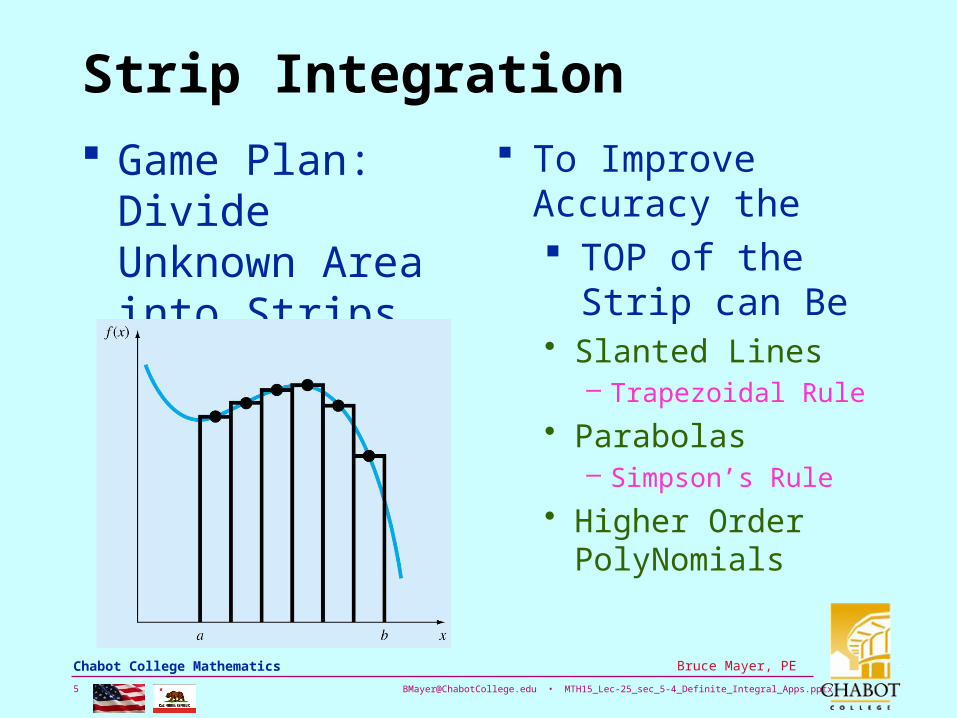
Strip Integration
Game Plan: Divide Unknown Area into Strips (or boxes), and Add Up
To Improve Accuracy the TOP of the Strip
can Be• Slanted Lines
– Trapezoidal Rule
• Parabolas– Simpson’s Rule
• Higher Order PolyNomials

[email protected] • MTH15_Lec-25_sec_5-4_Definite_Integral_Apps.pptx 6
Bruce Mayer, PE Chabot College Mathematics
Strip Integration Game Plan: Divide
Unknown Area into Strips (or boxes), and Add Up
To Improve Accuracy 1. Increase the
Number of strips; i.e., use smaller ∆x
2. Modify Strip-Tops– Slanted Lines (used
most often)– Parabolas– High-Order
Polynomials
Hi-No. of Flat-StripsWorks Fine.
[email protected] • MTH15_Lec-25_sec_5-4_Definite_Integral_Apps.pptx 7
Bruce Mayer, PE Chabot College Mathematics
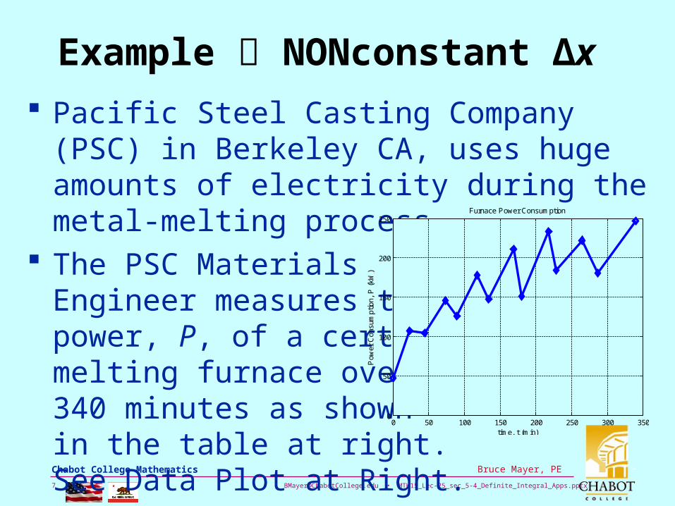
Example NONconstant ∆x
Pacific Steel Casting Company (PSC) in Berkeley CA, uses huge amounts of electricity during the metal-melting process.
The PSC Materials Engineer measures the power, P, of a certain melting furnace over 340 minutes as shown in the table at right. See Data Plot at Right.
0 50 100 150 200 250 300 3500
50
100
150
200
250
time, t (min)
Pow
er C
onsu
mpt
ion,
P (
kW)
Furnace Power Consumption

[email protected] • MTH15_Lec-25_sec_5-4_Definite_Integral_Apps.pptx 8
Bruce Mayer, PE Chabot College Mathematics
Example NONconstant ∆x
The T-table at Right displays the Data Collected by the PSC Materials Engineer
Recall from Physics that Energy (or Heat), Q, is the time-integral of the Power.
Use Strip-Integration to find theTotal Energy in MJ expended byThe Furnace during this processrun
Time (min)
Power (kW)
0 47 24 107 45 104 74 146 90 126
118 178 134 147 169 211 180 151 218 233 229 184 265 222 287 180 340 247

[email protected] • MTH15_Lec-25_sec_5-4_Definite_Integral_Apps.pptx 9
Bruce Mayer, PE Chabot College Mathematics
Example NONconstant ∆x
GamePlan for Strip Integration Use a Forward Difference
approach• ∆tn = tn+1 − tn
– Example: ∆t6 = t7 − t6 = 134 − 118 = 16min → 16min·(60sec/min) = 960sec
• Over this ∆t assume the P(t) is constant at Pavg,n =(Pn+1 + Pn)/2– Example: Pavg,6 = (P7 + P6)/2 =
(147+178)/2 = 162.5 kW = 162.5 kJ/sec
Time (min)
Power (kW)
0 47 24 107 45 104 74 146 90 126
118 178 134 147 169 211 180 151 218 233 229 184 265 222 287 180 340 247

[email protected] • MTH15_Lec-25_sec_5-4_Definite_Integral_Apps.pptx 10
Bruce Mayer, PE Chabot College Mathematics
Example NONconstant ∆x
The GamePlan Graphically• Note the
VariableWidth, ∆x,of the StripTops
t (minutes)
P (
kW)
MTH15 • Variable-Width Strip-Integration
0 50 100 150 200 250 300 3500
25
50
75
100
125
150
175
200
225Bruce May er, PE • 25Jul13
4x
9x

[email protected] • MTH15_Lec-25_sec_5-4_Definite_Integral_Apps.pptx 11
Bruce Mayer, PE Chabot College Mathematics
MA
TL
AB
Co
de
% Bruce Mayer, PE% MTH-15 • 25Jul13% XY_Area_fcn_Graph_6x6_BlueGreen_BkGnd_Template_1306.m%clear; clc; clf; % clf is clear figure%% The FUNCTIONxmin = 0; xmax = 350; ymin = 0; ymax = 225;x = [0 24 24 45 45 74 74 90 90 118 118 134 134 169 169 180 180 218 218 229 229 265 265 287 287 340]y = [77 77 105.5 105.5 125 125 136 136 152 152 162.5 162.5 179 179 181 181 192 192 208.5 208.5 203 203 201 201 213.5 213.5]% % The ZERO Lineszxh = [xmin xmax]; zyh = [0 0]; zxv = [0 0]; zyv = [ymin ymax];%% the 6x6 Plotaxes; set(gca,'FontSize',12);whitebg([0.8 1 1]); % Chg Plot BackGround to Blue-Green% Now make AREA Plotarea(x,y,'FaceColor',[1 0.6 1],'LineWidth', 3),axis([xmin xmax ymin ymax]),... grid, xlabel('\fontsize{14}t (minutes)'), ylabel('\fontsize{14}P (kW)'),... title(['\fontsize{16}MTH15 • Variable-Width Strip-Integration',]),... annotation('textbox',[.15 .82 .0 .1], 'FitBoxToText', 'on', 'EdgeColor', 'none', 'String', 'Bruce Mayer, PE • 25Jul13','FontSize',7)set(gca,'XTick',[xmin:50:xmax]); set(gca,'YTick',[ymin:25:ymax])set(gca,'Layer','top')

[email protected] • MTH15_Lec-25_sec_5-4_Definite_Integral_Apps.pptx 12
Bruce Mayer, PE Chabot College Mathematics
Example NONconstant ∆x
The NONconstant Strip-Width Integration is conveniently done in an Excel SpreadSheet
The 13 ∆Q strips Add up to 3456.69 MegaJoules of Total Energy Expended
n Time, t Power ∆t = 60*(tn+1-tn) Pavg=(Pn+1−Pn)/2 ∆Q= Pavg*∆t
(cnt) (min) (kW) (Sec) (kW) (kJ)
1 0 47
1 1440 77 110880
2 24 107
2 1260 105.5 132930
3 45 104
3 1740 125 217500
4 74 146
4 960 136 130560
5 90 126
5 1680 152 255360
6 118 178
6 960 162.5 156000
7 134 147
7 2100 179 375900
8 169 211
8 660 181 119460
9 180 151
9 2280 192 437760
10 218 233
10 660 208.5 137610
11 229 184
11 2160 203 43848012 265 22212 1320 201 26532013 287 18013 3180 213.5 67893014 340 247
3456.69Total Energy in MJ = (∑∆Q)/1000 =

[email protected] • MTH15_Lec-25_sec_5-4_Definite_Integral_Apps.pptx 13
Bruce Mayer, PE Chabot College Mathematics
Area Between Two Curves
Let f and g be continuous functions, the area bounded above by y = f (x) and below by y = g(x) on [a, b] is
• Provided that
• The Areal DifferenceRegion, R, Graphically
( ) ( )b
af x g x dx
( ) ( ) on , .f x g x a b ( )y g x
( )y f x
a b
R
x
y

[email protected] • MTH15_Lec-25_sec_5-4_Definite_Integral_Apps.pptx 14
Bruce Mayer, PE Chabot College Mathematics
Example Area Between Curves
Find the area between functions f & g over the interval x = [0,10]
The Graphsof f & g
10
25
58and
911
2
6
xxg
exf x
0 2 4 6 8 100
2
4
6
8
10
12
14
16
18
20
x
ylo
= (
-8/2
5)*
(x-5
)2 +1
0 •
yh
i = 1
1e-x
/6+
9
MTH15 • Area Between Curves
Bruce May er, PE • 25Jul13
911 6 xexf
10
25
58 2
x
xg

[email protected] • MTH15_Lec-25_sec_5-4_Definite_Integral_Apps.pptx 15
Bruce Mayer, PE Chabot College Mathematics
Example Area Between Curves
The process Graphically
x
ylo
= (
-8/2
5)*
(x-5
)2+
10
• y
hi =
11
e-x/
6 +9
MTH15 • Area Between Curves
0 2 4 6 8 100
2
4
6
8
10
12
14
16
18
20
x0 2 4 6 8 10
0
2
4
6
8
10
12
14
16
18
20
x0 2 4 6 8 10
0
2
4
6
8
10
12
14
16
18
20
Bruce May er, PE • 25Jul13Bruce May er, PE • 25Jul13 Bruce May er, PE • 25Jul13
− = 10
0
6 911 xe x dx
x
10
0
2
25
5810
10
0dxxgxf
[email protected] • MTH15_Lec-25_sec_5-4_Definite_Integral_Apps.pptx 16
Bruce Mayer, PE Chabot College Mathematics
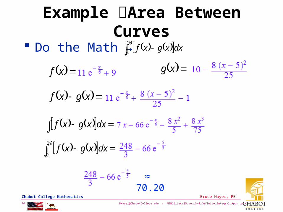
Example Area Between Curves
Do the Math → 10
0dxxgxf
xf xg
xgxf
dxxgxf
10
0dxxgxf
≈ 70.20

[email protected] • MTH15_Lec-25_sec_5-4_Definite_Integral_Apps.pptx 17
Bruce Mayer, PE Chabot College Mathematics
Example Area Between Curves
ThusAns
x
ylo
= (
-8/2
5)*
(x-5
)2+
10
• y
hi =
11
e-x/
6 +9
MTH15 • Area Between Curves
0 2 4 6 8 100
2
4
6
8
10
12
14
16
18
20
Bruce May er, PE • 25Jul13
A = 70.200
[email protected] • MTH15_Lec-25_sec_5-4_Definite_Integral_Apps.pptx 18
Bruce Mayer, PE Chabot College Mathematics
MA
TL
AB
Co
de
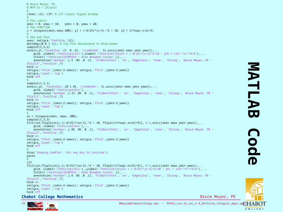
% Bruce Mayer, PE% MTH-15 • 25Jun13%clear; clc; clf; % clf clears figure window%% The Limitsxmin = 0; xmax = 10; ymin = 0; ymax = 20;% The FUNCTIONx = linspace(xmin,xmax,500); y1 = (-8/25)*(x-5).^2 + 10; y2 = 11*exp(-x/6)+9;% % the 6x6 Plotaxes; set(gca,'FontSize',12);whitebg([0.8 1 1]); % Chg Plot BackGround to Blue-Greensubplot(1,3,2)area(x,y1,'FaceColor',[1 .8 .4], 'LineWidth', 3),axis([xmin xmax ymin ymax]),... grid, xlabel('\fontsize{14}x'),ylabel('\fontsize{14}ylo = (-8/25)*(x-5)^2+10 • yhi = 11e^-^x^/^6+9'),... title(['\fontsize{16}MTH15 • Area Between Curves',]),... annotation('textbox',[.5 .05 .0 .1], 'FitBoxToText', 'on', 'EdgeColor', 'none', 'String', 'Bruce Mayer, PE • 25Jul13','FontSize',7)hold onset(gca,'XTick',[xmin:2:xmax]); set(gca,'YTick',[ymin:2:ymax])set(gca,'Layer','top')hold off%subplot(1,3,1)area(x,y2, 'FaceColor',[0 1 0], 'LineWidth', 3),axis([xmin xmax ymin ymax]),... grid, xlabel('\fontsize{14}x'),... annotation('textbox',[.15 .05 .0 .1], 'FitBoxToText', 'on', 'EdgeColor', 'none', 'String', 'Bruce Mayer, PE • 25Jul13','FontSize',7)hold onset(gca,'XTick',[xmin:2:xmax]); set(gca,'YTick',[ymin:2:ymax])set(gca,'Layer','top')hold off%xn = linspace(xmin, xmax, 500);subplot(1,3,3)fill([xn,fliplr(xn)],[(-8/25)*(xn-5).^2 + 10, fliplr(11*exp(-xn/6)+9)],'m'),axis([xmin xmax ymin ymax]),... grid, xlabel('\fontsize{14}x'),... annotation('textbox',[.85 .05 .0 .1], 'FitBoxToText', 'on', 'EdgeColor', 'none', 'String', 'Bruce Mayer, PE • 25Jul13','FontSize',7)hold onset(gca,'XTick',[xmin:2:xmax]); set(gca,'YTick',[ymin:2:ymax])set(gca,'Layer','top')hold off%disp('Showing SubPlot - Hit Any Key to Continue')pause%clffill([xn,fliplr(xn)],[(-8/25)*(xn-5).^2 + 10, fliplr(11*exp(-xn/6)+9)],'m'),axis([xmin xmax ymin ymax]),... grid, xlabel('\fontsize{14}x'),,ylabel('\fontsize{14}ylo = (-8/25)*(x-5)^2+10 • yhi = 11e^-^x^/^6+9'),... title(['\fontsize{16}MTH15 • Area Between Curves',]),... annotation('textbox',[.6 .05 .0 .1], 'FitBoxToText', 'on', 'EdgeColor', 'none', 'String', 'Bruce Mayer, PE • 25Jul13','FontSize',7)hold onset(gca,'XTick',[xmin:2:xmax]); set(gca,'YTick',[ymin:2:ymax])set(gca,'Layer','top')hold off

[email protected] • MTH15_Lec-25_sec_5-4_Definite_Integral_Apps.pptx 19
Bruce Mayer, PE Chabot College Mathematics
MuPAD Code
f := 11*exp(-x/6)+9g := (-8/25)*(x-5)^2+10fminusg := f-gAntiDeriv := int(fminusg, x)ABC := int(fminusg, x=0..10)float(ABC)

[email protected] • MTH15_Lec-25_sec_5-4_Definite_Integral_Apps.pptx 20
Bruce Mayer, PE Chabot College Mathematics
Example Net Excess Profit
The Net Excess Profit of an investment plan over another is given by
• Where dP1/dt & dP2/dt are the rates of profitability of plan-1 & plan-2
The Net Excess Profit (NEP) gives the total profit gained by plan-1 over plan-2 in a given time interval.
b
a
b
adtdtdPdtdPdttPtP 2121 ''

[email protected] • MTH15_Lec-25_sec_5-4_Definite_Integral_Apps.pptx 21
Bruce Mayer, PE Chabot College Mathematics
Example Net Excess Profit
Find the net excess profit during the period from now until plan-1 is no longer increasing faster than plan-2:
Plan-1 is an investment that is currently increasing in value at $500 per day and dP1/dt (P1’) is increasing instantaneously by 1% per day, as compared to plan-2 which is currently increasing in value at $100 per day and dP2/dt (P2’) is increasing instantaneously by 2% per day

[email protected] • MTH15_Lec-25_sec_5-4_Definite_Integral_Apps.pptx 22
Bruce Mayer, PE Chabot College Mathematics
Example Net Excess Profit
SOLUTION: The functions are each increasing
exponentially (instantaneously), with dP1/dt initially 500 and growing exponentially with k = 0.01, so that
Similarly, dP2/dt is initially 100 and growing exponentially with k = 0.02, so that
tedt
dP 01.01 500
tedt
dP 02.02 100
[email protected] • MTH15_Lec-25_sec_5-4_Definite_Integral_Apps.pptx 23
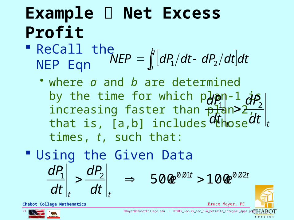
Bruce Mayer, PE Chabot College Mathematics
Example Net Excess Profit
ReCall theNEP Eqn• where a and b are determined
by the time for which plan-1 is increasing faster than plan-2, that is, [a,b] includes those times, t, such that:
Using the Given Data
b
adtdtdPdtdPNEP 21
tt dt
dP
dt
dP 21
tt
tt
eedt
dP
dt
dP 02.001.021 100500

[email protected] • MTH15_Lec-25_sec_5-4_Definite_Integral_Apps.pptx 24
Bruce Mayer, PE Chabot College Mathematics
Example Net Excess Profit
Dividing Both Sides of the InEquality
Taking the Natural Log of Both Side
Divide both Sides by 0.01 to Solve for t
tttt
tt
eee
ee 01.001.002.001.0
02.001.0
5100
100500
te t 01.05ln5ln 01.0
94.16001.0
5ln
01.0
5ln tt

[email protected] • MTH15_Lec-25_sec_5-4_Definite_Integral_Apps.pptx 25
Bruce Mayer, PE Chabot College Mathematics
Example Net Excess Profit
The plan-1 is greater than plan-2 from day-0 to day 160.94.
Thus after rounding the NEP covers the time interval [0,161]. The the NEP Eqn:
Doing the Calculus
dteeNEP tt days 161
days 0
02.001.0 100500
161
0
02.001.0161
0
02.001.0
02.0
100
01.0
500100500
tttt eedtee

[email protected] • MTH15_Lec-25_sec_5-4_Definite_Integral_Apps.pptx 26
Bruce Mayer, PE Chabot College Mathematics
Example Net Excess Profit
STATE: In the initial 161 days, the Profit from plan-1 exceeded that of plan-2 by approximately $80k
)0(02.0)0(01.0)161(02.0)161(01.0
02.0
100
01.0
500
02.0
100
01.0
500eeee
96.999,79
[email protected] • MTH15_Lec-25_sec_5-4_Definite_Integral_Apps.pptx 27
Bruce Mayer, PE Chabot College Mathematics
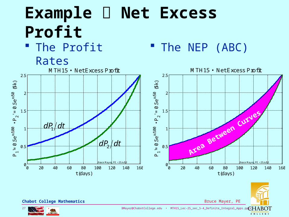
Example Net Excess Profit The Profit Rates The NEP (ABC)
0 20 40 60 80 100 120 140 1600
0.5
1
1.5
2
2.5
t (days)
P1'=
0.5
ex/
100 •
P2' =
0.5
ex/
50 (
$k)
MTH15 • Net Excess Profit
Bruce May er, PE • 25Jul13
0 20 40 60 80 100 120 140 1600
0.5
1
1.5
2
2.5
t (days)
P1'=
0.5
ex/
100
• P
2' = 0
.5e
x/50
($
k)
MTH15 • Net Excess Profit
Bruce May er, PE • 25Jul13
dtdP1
dtdP2Area Between Curves

[email protected] • MTH15_Lec-25_sec_5-4_Definite_Integral_Apps.pptx 28
Bruce Mayer, PE Chabot College Mathematics
MA
TL
AB
Co
de
% Bruce Mayer, PE% MTH-15 • 25Jun13%clear; clc; clf; % clf clears figure window%xmin = 0; xmax = 161; ymin = 0; ymax = 2.5;% The FUNCTIONx = linspace(xmin,xmax,500); y1 = .5*exp(x/100); y2 = .1*exp(x/50);% x in days • y's in $k%% the 6x6 Plotaxes; set(gca,'FontSize',12);whitebg([0.8 1 1]); % Chg Plot BackGround to Blue-Greenplot(x,y1, x,y2, 'LineWidth', 4),axis([xmin xmax ymin ymax]),... grid, xlabel('\fontsize{14}t (days)'), ylabel('\fontsize{14} P_1''= 0.5e^x^/^1^0^0 • P_2'' = 0.5e^x^/^5^0^ ($k)'),... title(['\fontsize{16}MTH15 • Net Excess Profit',]),... annotation('textbox',[.6 .05 .0 .1], 'FitBoxToText', 'on', 'EdgeColor', 'none', 'String', 'Bruce Mayer, PE • 25Jul13','FontSize',7)hold onset(gca,'XTick',[xmin:20:xmax]); set(gca,'YTick',[ymin:0.5:ymax])disp('Hit ANY KEY to show Fill')pause%xn = linspace(xmin, xmax, 500);fill([xn,fliplr(xn)],[.5*exp(xn/100), fliplr(.1*exp(x/50))],'m')hold off

[email protected] • MTH15_Lec-25_sec_5-4_Definite_Integral_Apps.pptx 29
Bruce Mayer, PE Chabot College Mathematics
Recall: Average Value of a fcn
Mathematically - If f is integrable on [a, b], then the average value of f over [a, b] is
Example Find the Avg Value:
Use Average Definition:
1( )
b
af x dx
b a
3/ 2( ) over 0,9 .f x x
9 3/ 2
0
1
9 0x dx
9
5/ 2
0
1 2
9 5
x
5/ 229
45 54
5

[email protected] • MTH15_Lec-25_sec_5-4_Definite_Integral_Apps.pptx 30
Bruce Mayer, PE Chabot College Mathematics
Example GeoTech Engineering
A Model for The rate at which sediment gathers at the delta of a river is given by• Where
– t ≡ the length of time (years) since study began– M ≡ the Mass of sediment (tons) accumulated
What is the average rate at which sediment gathers during the first six months of study?
)
32
3
tdt
dM

[email protected] • MTH15_Lec-25_sec_5-4_Definite_Integral_Apps.pptx 31
Bruce Mayer, PE Chabot College Mathematics
Example GeoTech Engineering
By the Avg Value eqn the average rate at which sediment gathers over the first six months (0.5 years)
No Integration Rule applies so try subsitution. Let
5.0
0
32
3
05.0
1
1dt
tVdttf
abV
b
a
32 tu
22
2232du
dtdt
dt
du
dt
dutu
dt
d

[email protected] • MTH15_Lec-25_sec_5-4_Definite_Integral_Apps.pptx 32
Bruce Mayer, PE Chabot College Mathematics
Example GeoTech Engineering
And
Then the Transformed Integral
Working the Calculus
43135.025.0
330302032
u
utu
4
3
5.0
0 2
3
05.0
1
32
3
05.0
1 u
u
t
t
du
uVdt
tV
434
3
4
3ln3
2
32
2
32 u
u
du
u
duV
8630.02877.033
4ln33ln4ln3
V

[email protected] • MTH15_Lec-25_sec_5-4_Definite_Integral_Apps.pptx 33
Bruce Mayer, PE Chabot College Mathematics
Example GeoTech Engineering
The average rate at which sediment was gathering for the first six months was 0.863 tons per year.
dM/dt along with its average value on [0,0.5]:
Equal Areas

[email protected] • MTH15_Lec-25_sec_5-4_Definite_Integral_Apps.pptx 34
Bruce Mayer, PE Chabot College Mathematics
WhiteBoard Work
Problems From §5.4• P46 → Worker Productivity• P60 → Cardiac Fluidic Mechanics

[email protected] • MTH15_Lec-25_sec_5-4_Definite_Integral_Apps.pptx 35
Bruce Mayer, PE Chabot College Mathematics
All Done for Today
DilBertIntegration

[email protected] • MTH15_Lec-25_sec_5-4_Definite_Integral_Apps.pptx 36
Bruce Mayer, PE Chabot College Mathematics
Bruce Mayer, PELicensed Electrical & Mechanical Engineer
Chabot Mathematics
Appendix
–
srsrsr 22

[email protected] • MTH15_Lec-25_sec_5-4_Definite_Integral_Apps.pptx 37
Bruce Mayer, PE Chabot College Mathematics

[email protected] • MTH15_Lec-25_sec_5-4_Definite_Integral_Apps.pptx 38
Bruce Mayer, PE Chabot College Mathematics

[email protected] • MTH15_Lec-25_sec_5-4_Definite_Integral_Apps.pptx 39
Bruce Mayer, PE Chabot College Mathematics
P5.4-46(b) Production Rates Cumulative Difference
• Qtot = 184/3 units
0 0.5 1 1.5 2 2.5 3 3.5 40
10
20
30
40
50
60
70
t (Hrs after 8am)
Q1'=
60
-2(t
-1)2 •
Q2' =
50
-5t
(un
its/h
r)
MTH15 • P5.4-46
Bruce May er, PE • 25Jul13
0 0.5 1 1.5 2 2.5 3 3.5 40
10
20
30
40
50
60
70
t (Hrs after 8am)
Q1'=
60
-2(t
-1)2 •
Q2' =
50
-5t
(un
its/h
r)
MTH15 • P5.4-46
Bruce May er, PE • 25Jul13
ABC = 184/3

[email protected] • MTH15_Lec-25_sec_5-4_Definite_Integral_Apps.pptx 40
Bruce Mayer, PE Chabot College Mathematics

[email protected] • MTH15_Lec-25_sec_5-4_Definite_Integral_Apps.pptx 41
Bruce Mayer, PE Chabot College Mathematics
[email protected] • MTH15_Lec-25_sec_5-4_Definite_Integral_Apps.pptx 42
Bruce Mayer, PE Chabot College Mathematics

[email protected] • MTH15_Lec-25_sec_5-4_Definite_Integral_Apps.pptx 43
Bruce Mayer, PE Chabot College Mathematics

[email protected] • MTH15_Lec-25_sec_5-4_Definite_Integral_Apps.pptx 44
Bruce Mayer, PE Chabot College Mathematics

[email protected] • MTH15_Lec-25_sec_5-4_Definite_Integral_Apps.pptx 45
Bruce Mayer, PE Chabot College Mathematics

[email protected] • MTH15_Lec-25_sec_5-4_Definite_Integral_Apps.pptx 46
Bruce Mayer, PE Chabot College Mathematics


