
Blown Film Extrusion: Experimental,
Modelling and Numerical Study
A thesis submitted in fulfilment of the requirements for the Degree of Doctor of Philosophy
Khokan Kanti Majumder B.Sc Eng (Chemical), PGrad Dip in IT
School of Civil, Environmental and Chemical Engineering
Science, Engineering and Technology Portfolio
RMIT University
March, 2008
Declaration
I certify that except where due acknowledgement has been made, the work is that of the
author alone; the work has not been submitted previously, in whole or in part, to qualify
for any other academic award; the content of the thesis is the result of work which has
been carried out since the official commencement date of the approved research
program; and, any editorial work, paid or unpaid, carried out by a third party is
acknowledged.
(Khokan Kanti Majumder)
Date: 18th
March, 2008

This research is dedicated to my grand father
SARAT CHANDRA MAJUMDER (Martyr)
who died in 1971 during the liberation war in Bangladesh
i
Acknowledgements
This thesis concludes a challenge in my life. I walked through a slippery road during this
journey. The knowledge and experience I have had from this journey could never have
been gained without the guidance and support of the following people:
Professor Sati N Bhattacharya, my senior supervisor: His guidance and constant care in this
research have led to the success of my study. For his expertise in melt rheology and
polymer processing, I got the opportunity to use various plastic processing equipments and
rheometers for this research. His curiosity and enthusiasm towards science and technology
inspired me to work as a researcher in polymer field.
Dr. Graham Hobbs, my supervisor in AMCOR Research & Technology: His constant
support inspired me to use the modern lab facilities for this blown film research at AMCOR
Research & Technology. His technical advice opened my eyes for a root level study of
blown film extrusion.
Dr. Yan Ding, my supervisor in the School of Mathematics and Geospatial Sciences: She
helped me to understand the numerical techniques of the blown film modelling and
simulation. Without her help, it would have been impossible to simulate the blown film
processing.
ii
Mr Ranajit Majumder and Mrs Mamata Rani Majumder, my parents: Without their
“ruthless” push, support, love and blessings, I couldn’t have finished my education.
Dr. Kali Pada Majumder, Mr. Ramaprasad Majumder and Mr. Uttam Kumar Majumder,
my brothers: They supported and encouraged me at all times about my study and other
occasions.
Bithi Kana Paul, my wife: I would like to acknowledge her patience during my study. I
would like to thank Dr. Manoranjan Paul, Mr. Nikhil Chandra Paul and Mrs. Tulshi Rani
Paul for their encouragement.
Ms. Allison Noel and Mr. Steve Barnett in AMCOR Research & Technology and Mr. Bob
Havelka in AMCOR Flexibles, Moorabbin, Melbourne: for their technical support to
organise and complete all laboratory activities scheduled for this research.
Assoc/Prof. John Shepherd and Dr. John Gear of School of Mathematics and Geospatial
Sciences: for teaching me the continuum fluid mechanics.
Dr. Sumanta Raha: for his technical advice in experimentations and data analysis.
Mr. Mike Allan and Mr. Andrew Chryss: for their constant help in the laboratory to run the
equipments and data acquisitions.

iii
Dr Ranjit Prasad and Dr. Deeptangshu Chaudhary: for their help in my experimental works.
I would also like to thank all postgraduate students of Rheology and Materials Processing
Centre for their time and support in several social activities.
iv
Abstract
It is well known that most polymers are viscoelastic and exhibit independent rheological
characteristics due to their molecular architecture. Based on the melt rheological response,
polymers behave differently during processing. Therefore, it is very useful to understand
the molecular structure and rheological properties of the polymers before they are selected
for processing. Simulation is a useful tool to investigate the process characteristics as well
as for scaling up and optimisation of the production. This thesis correlates rheological data
into a non-linear blown film model that describes the stress and cooling-induced
morphological transformations in the axial and flow profiles of the blown films. This will
help to improve the physical and mechanical properties of the films in a cost effective way,
which will in turn be of great benefit to the food and packaging industries.
In this thesis, experimental and numerical studies of a blown film extrusion were carried
out using two different low-density polyethylenes(LDPEs). In the experiment, the key
parameters measured and analysed were molecular, rheological and crystalline properties of
the LDPEs. Dynamic shear rheological tests were conducted using a rotational rheometer
(Advanced Rheometric Expansion System (ARES)). Steady shear rheological data were
obtained from both ARES and Davenport capillary rheometer. Time temperature
superposition (TTS) technique was utilized to determine the flow activation energy, which
determines the degree of LCB. Modified Cross model was used to obtain the zero shear
viscosity (ZSV). Melt relaxation time data was fitted into the Maxwell model to determine

v
average and longest relaxation time. Thermal analysis was carried out using modulated
differential scanning calorimetry (MDSC) and TA instrument software (MDSC-2920). The
crystalline properties data obtained from the MDSC study were also verified using the wide
angle X-ray diffraction (WAXD) data from the Philips X-ray generator.
In the numerical study, blown film simulation was carried out to determine the bubble
characteristics and freeze line height (FLH). A new rheological constitutive equation was
developed by combining the Hookean model with the well known Phan-Thien and Tanner
(PTT) model to permit a more accurate viscoelastic behaviour of the material. For
experimental verification of the simulation results, resins were processed in a blown film
extrusion pilot plant using identical die temperatures and cooling rates as used in the
simulation study.
Molecular characteristics of both LDPEs were compared in terms of their processing
benefit in the film blowing process. Based on the experimental investigation, it was found
that molecular weight and its distribution, degree of long chain branching and cooling rate
play an important role on melt rheology, molecular orientation, blown film processability,
film crystallinity and film properties. Effect of short chain branching was found
insignificant for both LDPEs.
Statistical analysis was carried out using MINITAB-14 software with a confidence level of
95% to determine the effect of process variables (such as die temperature and cooling rate)
vi
on the film properties. Film properties of the LDPEs were found to vary with their
molecular properties and the process variables used.
Blown film model performance based on the newly established PTT-Hookean model was
compared with that based on the Kelvin model. Justification of the use of PTT-Hookean
model is also reported here using two different material properties. From the simulation
study, it has been found that predictions of the blown film characteristics conformed very
well to the experimental data of this research and previous studies using different materials
and different die geometries.
Long chain branching has been found as the most prominent molecular parameter for both
LDPEs affecting melt rheology and hence the processibility. Die temperature and cooling
rate have been observed to provide similar effect on the tear strength and shrinkage
properties of blown film for both LDPEs. In comparison to the Kelvin model, the PTT-
Hookean model is better suited for the modelling of the film blowing process. It has also
been demonstrated in this study that the PTT-Hookean model conformed well to the
experimental data near the freeze line height and is suitable for materials of lower melt
elasticity and relaxation time.
vii
Contents
Acknowledgements………………………………………………………………………...i
Abstract……………………………………………………………………………………iv
CHAPTER 1:
Introduction..........................................................................................................................1
1.1 Global and local market of the plastic film............................................................1
1.2 Materials for packaging applications .....................................................................3
1.3 Plastic film processing ...........................................................................................4
1.3.1 Blown film processing ...................................................................................4
1.3.2 Optimisation of the blown film production ...................................................6
1.4 Aim and objectives of this research.......................................................................8
1.5 Scopes of this research...........................................................................................8
1.6 Description of the chapters ....................................................................................9
CHAPTER 2:
Fundamentals of Rheological, Crystalline and Film Properties Characterisations ....11
2.1 Blown film process ..............................................................................................11
2.2 Melt rheology.......................................................................................................14
2.2.1 Shear rheology .............................................................................................14
2.2.1.1 Dynamic (oscillatory) shear rheology......................................................15
2.2.1.2 Molecular structure and viscoelasticity ...................................................16
2.2.1.3 Steady shear rheology..............................................................................18
2.2.1.4 Steady shear viscosity of polyethylene....................................................19
2.2.2 Extensional rheology ...................................................................................21
2.2.2.1 Extensional (elongational) viscosity of polyethylene..............................22
2.2.2.2 Uniaxial extensional test..........................................................................24
2.2.2.2.1 Meissner-type rheometer ...................................................................25
2.2.3 Effect of branching on melt rheology ..........................................................27
2.3 Wide angle X-ray scattering (WAXD) ................................................................29
viii
2.3.1 WAXD of semicrystalline polymer .............................................................30
2.3.2 WAXD of blown polyethylene film ............................................................31
2.4 Thermal analysis ..................................................................................................33
2.4.1 Thermal analysis of polyethylene ................................................................35
2.5 Blown film properties ..........................................................................................36
2.5.1 Mechanical properties..................................................................................38
2.5.1.1 Tensile strength........................................................................................38
2.5.1.2 Tear strength ............................................................................................39
2.5.1.3 Impact strength ........................................................................................40
2.5.2 Optical (haze and gloss) properties..............................................................41
2.5.3 Shrinkage properties ....................................................................................42
2.6 Summary..............................................................................................................43
CHAPTER 3:
Blown Film Modelling and Simulation ............................................................................45
3.1 Background..........................................................................................................45
3.2 Fundamental Film Blowing Equations ................................................................47
3.3 Fundamental of the Rheological Constitutive Equation ......................................49
3.3.1 Deformations in the Film Blowing Process .................................................51
3.4 Rheological Constitutive Equations Available in the Literature .........................53
3.4.1 Newtonian Model ........................................................................................53
3.4.2 Power Law Model........................................................................................55
3.4.3 Elastic Model ...............................................................................................62
3.4.4 Maxwell Model............................................................................................63
3.4.5 Viscoplastic-Elastic Modelling....................................................................64
3.4.6 Viscoelastic Model ......................................................................................65
3.4.7 Crystallization Model ..................................................................................67
3.4.8 Dynamic Modelling .....................................................................................68
3.5 Summary..............................................................................................................70

ix
CHAPTER 4:
Materials, Equipments and Experimental Techniques ..................................................71
4.1 Materials ..............................................................................................................71
4.2 Molecular properties ............................................................................................71
4.2.1 Gel permeation chromatography (GPC) ......................................................72
4.3 Rheological measurements ..................................................................................73
4.3.1 Shear rheology .............................................................................................74
4.3.1.1 Measurement of dynamic shear rheology................................................74
4.3.1.1.1 Parallel plate rheometer .....................................................................75
4.3.1.1.2 Plaque preparation .............................................................................77
4.3.1.1.3 Experimentation with ARES rheometer ............................................77
4.3.1.2 Steady shear rheology..............................................................................79
4.3.1.2.1 Parallel plate rheometer (ARES rheometer) ......................................79
4.3.1.2.2 Capillary rheometer ...........................................................................80
4.3.1.2.3 Davenport Ram extruder....................................................................81
4.3.2 Extensional rheology ...................................................................................82
4.3.2.1 Measurement of the extensional viscosity ...............................................82
4.3.2.1.1 Experimentation with RME rheometer..............................................83
4.4 Experimentation with Wide angle X-ray Diffraction (WAXD) ..........................85
4.5 Experimentation with Modulated Differential Scanning Calorimetry (MDSC) .85
4.6 Blown film production.........................................................................................87
4.6.1 Extruder geometries and process parameters...............................................89
4.7 Measurements of the blown film properties ........................................................90
4.7.1 Tensile strength............................................................................................90
4.7.2 Tear strength ................................................................................................91
4.7.3 Dart impact strength.....................................................................................92
4.7.4 Shrinkage properties ....................................................................................93
4.7.5 Optical properties (haze and gloss)..............................................................95
4.8 Summary..............................................................................................................96
x
CHAPTER 5:
Error Analysis ....................................................................................................................97
5.1 Dynamic shear measurements .............................................................................97
5.1.1 Linear viscoelastic region ............................................................................98
5.1.2 Thermal degradation ....................................................................................99
5.1.3 Variation of the parallel plates...................................................................100
5.1.4 Data consistency ........................................................................................101
5.2 Steady shear measurements ...............................................................................103
5.2.1 Parallel plates rheometer............................................................................103
5.2.1.1 Variation of shear rate............................................................................104
5.2.1.2 Thermal degradation ..............................................................................105
5.2.1.3 Flow instabilities....................................................................................106
5.2.2 Capillary rheometer ...................................................................................106
5.2.2.1 Wall slip.................................................................................................107
5.2.2.2 Melt fracture ..........................................................................................108
5.2.2.3 Temperature variation............................................................................109
5.2.2.4 Thermal degradation ..............................................................................110
5.3 Extensional rheological measurement ...............................................................111
5.3.1 Time delay .................................................................................................111
5.3.2 Force deviation ..........................................................................................112
5.4 WAXD study .....................................................................................................113
CHAPTER 6:
Results and Discussion of Rheological, Thermal, and Crystalline Properties ...........115
6.1 Molecular properties of the LDPEs ...................................................................115
6.2 Rheological properties .......................................................................................117
6.2.1 Shear rheology ...........................................................................................117
6.2.1.1 Dynamic shear rheology ........................................................................117
6.2.1.1.1 Effect of short chain branching........................................................118
6.2.1.1.2 Effect of molecular weight (Mw) .....................................................120
6.2.1.1.3 Linear viscoelastic properties of the LDPEs....................................121

xi
6.2.1.2 Zero shear viscosity (ZSV) ....................................................................124
6.2.1.3 Flow activation energy (FAE) ...............................................................126
6.2.1.4 Melt relaxation time...............................................................................129
6.2.1.5 Melt flow instabilities ............................................................................133
6.3 Extensional rheology .........................................................................................135
6.4 Thermal analysis ................................................................................................139
6.5 WAXD analysis .................................................................................................144
6.6 Summary............................................................................................................148
CHAPTER 7:
Establishment of a Rheological Constitutive Equation and Results of Blown Film
Simulation .……………………………………………………………………………....150
7.1 Governing equations ..........................................................................................150
7.1.1 Fundamental film blowing equations ........................................................151
7.1.2 Summary of the rheological constitutive equations used by the previous
studies 154
7.1.3 Rheological constitutive equations developed in this study ......................156
7.1.4 Development of the blown film equations.................................................158
7.2 Numerical techniques ........................................................................................161
7.2.1 Boundary conditions ..................................................................................162
7.2.2 Materials and process parameters at the die exit .......................................162
7.3 Results and discussion .......................................................................................163
7.3.1 Prediction of bubble characteristics ...........................................................164
7.3.1.1 Heat transfer coefficient.........................................................................166
7.3.1.2 Experimental verification ......................................................................166
7.3.2 Model predictions of stress and deformation rate......................................169
7.3.3 Justification of the use of the Hookean model with the PTT model..........171
7.4 Comparison study of the Kelvin and the PTT-Hookean model.........................175
7.5 Summary............................................................................................................181

xii
CHAPTER 8:
Statistical Analysis of the Film Properties.....................................................................182
8.1 Basis of the statistical analysis...........................................................................182
8.2 Mechanical properties........................................................................................183
8.2.1 Tensile strength..........................................................................................183
8.2.2 Tear strength ..............................................................................................186
8.2.3 Impact strength ..........................................................................................190
8.3 Shrinkage properties ..........................................................................................192
8.4 Optical (haze and gloss) properties....................................................................195
8.5 Summary............................................................................................................199
CHAPTER 9:
Conclusions and Recommendations...............................................................................201
9.1 Rheological properties .......................................................................................201
9.2 Crystalline properties .........................................................................................202
9.3 Blown film modelling and simulation ...............................................................202
9.4 Blown film properties ........................................................................................203
9.5 Recommendations for future work ....................................................................204
Bibliography……………………………………………………………………………...205
Appendix…………………………………………………………………………………213
List of symbols used in blown film modelling…………………….…………………....246
List of Publications arising from this research...………………………………………248

xiii
List of Tables
Table 4-1: Characteristics of the LDPE resins used for rheology and film production.......71
Table 4-2: ASTM D882 test conditions for tensile strength of the film..............................90
Table 4-3: ASTM D1922 test conditions for tear strength of the film ................................92
Table 4-4: ASTM D1709 test conditions for dart impact strength of the film ....................93
Table 4-5: ASTM D2732-03 test conditions for shrinkage of the film ...............................94
Table 4-6: ASTM D1003 test conditions for haze properties of the film............................95
Table 6-1: Molecular characteristics of the LDPEs obtained from GPC study.................117
Table 6-2: Zero shear viscosity of Pol-1............................................................................125
Table 6-3 : Zero shear viscosity of Pol-2...........................................................................126
Table 6-4 : Relaxation time of Pol-1 at different temperatures .........................................132
Table 6-5 : Relaxation time of Pol-2 at different temperatures .........................................132
Table 6-6 : Strain hardening parameter of the LDPEs at different temperatures and different
using different extensional viscosity..................................................................................137
Table 6-7 : Thermal and crystalline properties of the films processed at 200°C...............141
Table 7-1: Summary of the previous rheological constitutive equations used in blown film
model and their limitations ................................................................................................154
Table 7-2: Rheological and processing parameters of the resins used in the modelling ..163
Table 7-3: Comparison of the bubble characteristics of the processed film at FLH
(Majumder et al., 2007b) ...................................................................................................169
Table 8-1: Effect of temperature and cooling rate on the tensile strength (Appendix Figure
A3-13)................................................................................................................................186
Table 8-2: Crystalline properties of the blown films at 210°C (die temperature) .............186
Table 8-3: Effect of temperature and cooling rate on the tear strength (Appendix Figure A3-
14) ......................................................................................................................................190
Table 8-4: Effect of temperature and cooling rate on the shrinkage properties (Appendix
Figure A3-15) ....................................................................................................................195
Table 8-5: Effect of temperature and cooling rate on the haze properties (Appendix Figure
A3-16)................................................................................................................................198
Table 8-6: Effect of temperature and cooling rate on the gloss properties (Appendix Figure
A3-17)................................................................................................................................199

xiv
Table A1-1: Extrusion data sheet for film production………………………………........213
Table A1-2: Experimental data of MA-3 (Muke et al., 2003) …………………………...214
Table A1-3: Pilot plant data of Pol-1(Majumder et al., 2007b)…………………………..214
Table A2-1: Tensile strength of Pol-1 and Pol-2 film………………………….…………216
Table A2-2: Tear strength of Pol-1 and Pol-2 film………………………………….........216
Table A2-3: Impact strength of Pol-1 and Pol-2 film……………………………….........217
Table A2-4: Shrinkage length of Pol-1 and Pol-2 film……………………………….......217
Table A2-5: Shrinkage properties of Pol-1 and Pol-2 film………………………….........218
Table A2-6: Haze properties of Pol-1 and Pol-2 film……………………………….........218
Table A2-7: Gloss properties of Pol-1 and Pol-2 film………………………………........219
List of Figures
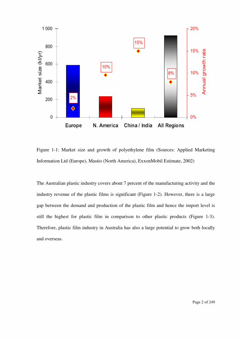
Figure 1-1: Market size and growth of polyethylene film (Sources: Applied Marketing
Information Ltd (Europe), Mastio (North America), ExxonMobil Estimate, 2002) .............2
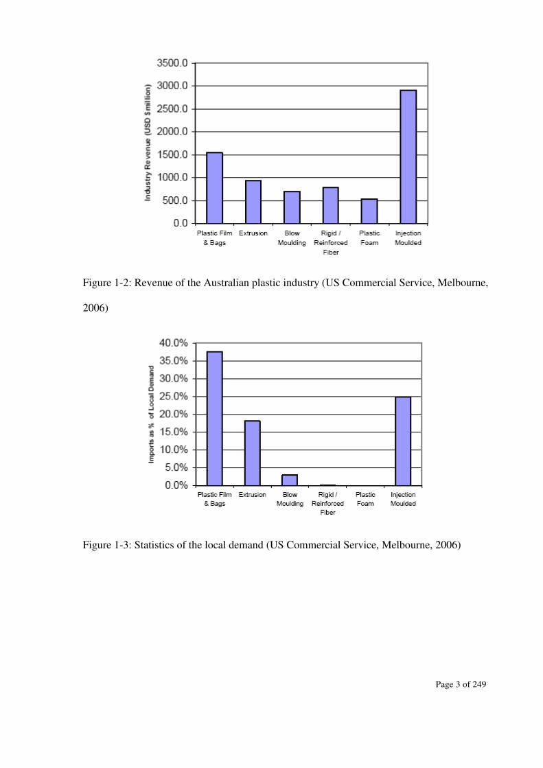
Figure 1-2: Revenue of the Australian plastic industry (US Commercial Service,
Melbourne, 2006)...................................................................................................................3
Figure 1-3: Statistics of the local demand (US Commercial Service, Melbourne, 2006) .....3
Figure 2-1: Schematic Diagram of the blown film process along with surface coordinates
and free body diagram of the forces. ...................................................................................13
Figure 2-2: Shear relaxation modulus versus time of a low-density polyethylene at 150°C
(Macosko, 1994). The solid line is the sum of the relaxation times obtained by Laun,
(1978)...................................................................................................................................17
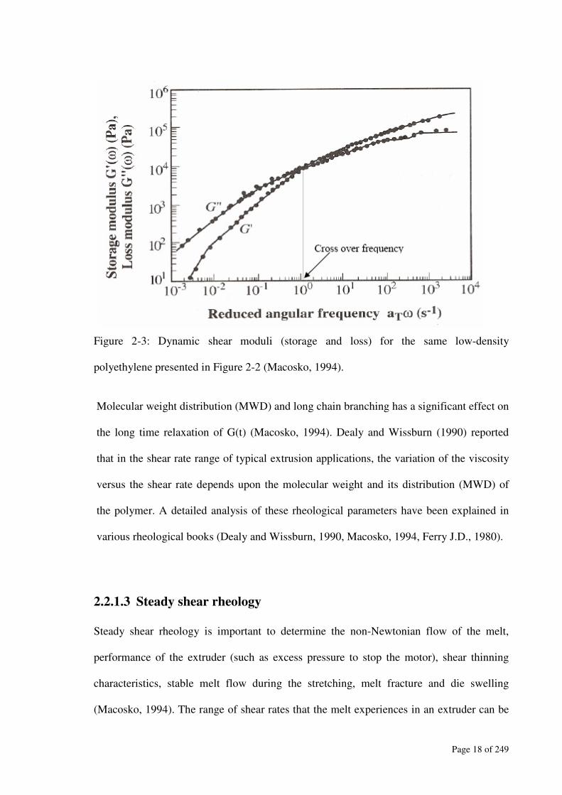
Figure 2-3: Dynamic shear moduli (storage and loss) for the same low-density polyethylene
presented in Figure 2-2 (Macosko, 1994). ...........................................................................18
Figure 2-4: Steady shear viscosity of pure polyethylene (7.4, 31, 6.8 and 3.5 are the MWD
of LDPE1, LDPE2, LDPE3 and LLDPE, respectively) at 190°C (Micic and Bhattacharya,
2000). ...................................................................................................................................20
Figure 2-5: Extensional viscosity versus tensile stress of three different LDPEs (Dealy and
Wissburn, 1990)...................................................................................................................23

xv
Figure 2-6: Extensional viscosity of LDPE at different strain rates at 150°C (Münstedt et
al., 1998). .............................................................................................................................24
Figure 2-7: Schematic diagram of uniaxial stretching using the Meissner-type extensional
rheometer. ............................................................................................................................25
Figure 2-8: Schematic of the extension produced during stretching flows..........................26
Figure 2-9: Schematic of X-Ray diffraction ........................................................................29
Figure 2-10: WAXD pattern of partially ordered polyethylene-(a) Baker and Windle
(2001); and (b) McFaddin et al (1993). ...............................................................................31
Figure 2-11: Morphological models of row-nucleated structure of polyethylene- a) low-
stress condition; and b) high-stress condition (Keller and Machin, 1967). .........................32
Figure 2-12: Shish kebab morphology (Abhiraman, 2003).................................................33
Figure 2-13: Thermograms (heating cycle) of three different polyethylene. ......................36
Figure 2-14: Schematic of morphological developments and structure-tear relationship of
polyethylene (Zhang et al., 2004). .......................................................................................39
Figure 3-1: Blown film production at AMCOR pilot plant ................................................46
Figure 3-2: Film geometry (a) Element of the film with force and (b) Curvature of the film
(Luo and Tanner, 1985). ......................................................................................................48
Figure 3-3: Coordinate systems describing the deformation of a bubble (Khonakdar et al.,
2002). ...................................................................................................................................50
Figure 3-4: A typical bubble shape for Newtonian fluid (Luo and Tanner, 1985)..............54
Figure 3-5: Extensional viscosity vs. extension rate for high-density polyethylene in biaxial
stretching: Q = 20.93 g/min, VO = 0.377 cm/sec, VL/V0 = 36.7, P∆ = 0.0109 psi (Han and
Park, 1975b).........................................................................................................................56
Figure 3-6: Extensional viscosity vs. extension rate for polypropylene in biaxial stretching:
Q = 13.88 g/min, VO = 0.258 cm/sec, VL/V0 = 67.2, P∆ = 0.0051 psi (Han and Park,
1975b). .................................................................................................................................56
Figure 3-7: Extensional viscosity vs. extension rate for low-density polyethylene in biaxial
stretching: Q = 18.10 g/min, VO = 0.346 cm/sec, VL/V0 = 28.9, P∆ = 0.0058 psi (Han and
Park, 1975b).........................................................................................................................57
xvi
Figure 3-8: Comparison of the experimentally observed bubble shape (a/a0) with the
theoretically predicted one for high-density polyethylene. Extrusion conditions: T=200°C,
Q=20.93g/min, n=0.79, V0=0.346cm/sec, VL/V0=17.5, P∆ =0.0187psi (Han and Park,
1975a). .................................................................................................................................58
Figure 3-9: Comparison of the experimentally observed bubble shape (a/a0) with the
theoretically predicted one for low-density polyethylene. Extrusion conditions: T=200°C,
Q=18.10g/min, n=1.28, V0=0.377cm/sec, VL/V0=12.4, P∆ =0.0079psi (Han and Park,
1975a). .................................................................................................................................58
Figure 3-10: Comparison of the experimentally determined film thickness (h/h0) with the
theoretically predicted one for high-density polyethylene (HDPE). Extrusion conditions
same as in Figure 3-9. ..........................................................................................................59
Figure 3-11: Comparison of the experimentally determined film thickness (h/h0) with the
theoretically predicted one for high-density polyethylene (LDPE). Extrusion conditions
same as in Figure 3-10. ........................................................................................................59
Figure 3-12: Calculated variation of blow-up ratio and film thickness versus axial distance
from the die head (Khonakdar et al., 2002). ........................................................................61
Figure 3-13: The total stress component versus axial distance from die exit (Khonakdar et
al., 2002). .............................................................................................................................62
Figure 3-14: Dimensionless radius, temperature and velocity profiles for elastic model (a is
the dimensionless bubble radius,ϕ is the dimensional temperature based on elastic modulus
and u is the dimensionless film speed). ...............................................................................63
Figure 4-1: Gel Permeation Chromatography (GPC) unit at the Rheology and Material
Processing Centre (RMPC) laboratory. ...............................................................................73
Figure 4-2: Schematic of a parallel plate rheometer (Macosko, 1994) ..............................75
Figure 4-3: Wabash instrument at RMPC laboratory. .........................................................77
Figure 4-4 : ARES rheometers at RMPC laboratory ...........................................................78
Figure 4-5: Step shear rate test of Pol-1 at a shear rate of 0.1s-1
and at 190°C. ..................80
Figure 4-6 : Davenport Ram Extruder at RMPC laboratory................................................81
Figure 4-7: Schematic of the uniaxial extension using the Meissner-type rheometer.........83
Figure 4-8 : RME rheometer at RMPC laboratory. .............................................................84
Figure 4-9: Phillips X-Ray generator at RMPC laboratory .................................................85
xvii
Figure 4-10: TA instrument (MDSC-2920) at RMPC laboratory .......................................86
Figure 4-11: Blown film production using the Advanced Blown Film Extrusion System at
AMCOR Research & Technology, Melbourne. ..................................................................87
Figure 4-12 : Instron- 4400 at AMCOR Research & Technology, Melbourne. ..................91
Figure 4-13: Elmendorf Tearing Tester (No.1653) at AMCOR Research & Technology,
Melbourne. ...........................................................................................................................92
Figure 4-14: Dart Impact Tester at RMPC laboratory. ........................................................93
Figure 4-15: Shrinkage testing silicone oil bath at AMCOR Research & Technology,
Melbourne. ...........................................................................................................................94
Figure 4-16: Schematic of gloss meter. ...............................................................................95
Figure 5-1 : Determination of linear viscoelastic strain of the resins (Pol-1 and Pol-2) .....98
Figure 5-2: Dynamic time sweep test of the LDPEs (Pol-1 and Pol-2) at 200°C
(frequency=10 rad/s and strain=10%)................................................................................100
Figure 5-3: Dynamic frequency sweep of Pol-2 at 210°C using 25mm and 50mm plates
geometries. .........................................................................................................................101
Figure 5-4: Dynamic shear rheology of the LDPEs – (a) Pol-1, and (b) Pol-2 obtained from
two different runs at 200°C................................................................................................102
Figure 5-5: Determination of the instrumental sensitivity from the data presented in Figure
5-4a. ...................................................................................................................................103
Figure 5-6: Viscosity correction of Pol-1 data (obtained at 200°C from ARES rheometer)
using Equation 5-2. ............................................................................................................105
Figure 5-7: Determination of time for a steady rate sweep test of Pol-1 at 200°C............106
Figure 5-8: Correction of Capillary rheometer data of Pol-1 obtained at 190°C. .............108
Figure 5-9: Correction of Capillary rheometer data of Pol-1 at 190°C .............................109
Figure 5-10: Capillary data of Pol-1 at 200°C obtained from two different runs..............110
Figure 5-11: Extensional data of Pol-1 at 140°C and three different stretching rates (0.1s-1
,
0.5s-1
and 1.0s-1
) .................................................................................................................112
Figure 5-12: Comparison of extensional data (stretching rate=1.0s-1
) of Pol-1 at 140°C. 113
Figure 5-13: WAXD study of Pol-1 film in MD obtained at die temperature=200°C and
blower setting=2.6. ............................................................................................................114
Figure 6-1: Gel permeation chromatography traces for Pol-1 and Pol-2. .........................116
xviii
Figure 6-2: Effect of short chain branching on complex viscosity at 200°C.....................119
Figure 6-3: Effect of short chain branching on phage angle at 200°C ..............................119
Figure 6-4: Phase angle of Pol-1 and Pol-2 as a function of frequency obtained
at 200°C. ............................................................................................................................121
Figure 6-5: Dynamic shear rheology of Pol-1 and Pol-2 at 200°C....................................122
Figure 6-6: Recoverable shear strain of Pol-1 and Pol-2 at 200°C...................................123
Figure 6-7: Steady shear viscosity of Pol-1 and Pol-2 at 190°C using modified Cross model
and steady shear experiment. .............................................................................................125
Figure 6-8: Dynamic frequency temperature sweep data of (a) Pol-1 and (b) Pol-2
(Majumder et al., 2007a)....................................................................................................127
Figure 6-9: Shifting of storage modulus of Pol-1 and Pol-2 to a reference temperature..128
Figure 6-10: Shift factor, aT versus 1/T of Pol-1 and Pol-2 (Majumder et al., 2007a) ......128
Figure 6-11: Relaxation spectrum of Pol-1 and Pol-2 at 200°C according to Maxwell
model and shear relaxation experiment (Majumder et al., 2007a). ...................................129
Figure 6-12: Storage modulus of Pol-1 and Pol-2 using Maxwell model (Equations 6-5 and
6-6) and experimental data (Majumder et al., 2007a)........................................................131
Figure 6-13: First normal stress coefficient of Pol-1 and Pol-2 at 200°C. ........................134
Figure 6-14: Melt flow instability of Pol-1 and Pol-2 at 200°C. ......................................135
Figure 6-15: Extensional viscosity (at 0.1 S-1
) of Pol-1and Pol-2 at 140°C and 150°C...136
Figure 6-16: Extensional viscosity (at 0.1s-1
) of Pol-1 at 140°C, 150°C and 170°C.........138
Figure 6-17: Extensional viscosity (at 0.1s-1
) of Pol-2 at 140°C, 150°C and 170°C.........138
Figure 6-18: MDSC thermogram of Pol-1 and Pol-2 before processing, a) Pellet and b)
Plaque.................................................................................................................................140
Figure 6-19: MDSC thermogram of Pol-1 and Pol-2 film obtained at 200°C and at cooling
rate (BS: 2.4)......................................................................................................................142
Figure 6-20: MDSC thermogram of Pol-1 film obtained at 200°C (die temperature) and at
four different cooling rates (BS: 2.4, 2.6, 2.8 and 3.0). .....................................................142
Figure 6-21: MDSC thermogram of Pol-2 film obtained at 200°C (die temperature) and at
four different cooling rates (BS: 2.4, 2.6, 2.8 and 3.0). .....................................................143
Figure 6-22: WAXD data of Pol-1 and Pol-2
(sample type is plaque in a rotational holder)....................................................................145
xix
Figure 6-23: WAXD plot of Pol-1((a) and (b)) and Pol-2((c) and (d)) films processed at
200°C (die temperature) and different blower settings (2.4, 2.6, 2.8 and 3.0). .................147
Figure 7-1: Development of the Blown film model and computational technique. ..........151
Figure 7-2: Effect of Deborah number (De0=0
0
r
vλ
) on the bubble shape as – (a) Pol-1,
(b) Pol-2 .............................................................................................................................165
Figure 7-3: Prediction of the heat transfer coefficient of Pol-1 using Equation 7-32. ......166
Figure 7-4: Verification of modelling outputs with the experimental data of Muke et al
(2003) and this study for-(a) bubble diameter; (b) film temperature; (c) film thickness..169
Figure 7-5: PTT-Hookean model prediction of the stresses in the machine (MD) and
transverse directions (TD) for Pol-1, respectively.............................................................170
Figure 7-6: PTT-Hookean model prediction of the strain rate in the machine (MD) and
transverse directions (TD) for Pol-1, respectively.............................................................171
Figure 7-7: Investigation of modelling outputs of the resins using PTT and PTT-Hookean
model and identical processing parameters- (a) bubble diameter of Pol-1; (b) bubble
diameter of Pol-2; (c) Film thickness of Pol-1; and (d) film thickness of Pol-2. ..............173
Figure 7-8: Effect of Deborah no (De0=λv0/r0) of Pol-2 in the prediction of blown film
thickness using PTT model and present study...................................................................175
Figure 7-9: Predictions of blown film characteristics and comparison with the experimental
data, (a) bubble diameter; and (b) film thickness. .............................................................177
Figure 7-10: Predictions of film temperature (a) and heat transfer coefficient (b)............178
Figure 7-11: Predictions of strain rates, (a) in the machine direction (MD); and (b) in the
transverse direction (TD). ..................................................................................................180
Figure 8-1: Interaction plot for tensile strength of Pol-1, a) in MD, and b) in TD............184
Figure 8-2: Interaction plot for tensile strength of Pol-2, a) in MD, and b) in TD............185
Figure 8-3: Interaction plot for tear strength of Pol-1, a) in MD, and b) in TD.. ..............187
Figure 8-4: Interaction plot for tear strength of Pol-2, a) in MD, and b) in TD. ...............189
Figure 8-5: Interaction plot of impact strength of Pol-1....................................................191
Figure 8-6 : Interaction plot of impact strength of Pol-2. .................................................191
Figure 8-7: Interaction plot for shrinkage properties of Pol-1, a) in MD, and b) in TD....193
xx
Figure 8-8: Interaction plot for shrinkage properties of Pol-2, a) in MD, and b) in TD....194
Figure 8-9: Interaction plot for haze properties of Pol-1. ..................................................197
Figure 8-10: Interaction plot for haze properties of Pol-2. ................................................197
Figure 8-11: Interaction plot for gloss properties of Pol-1. ...............................................198
Figure 8-12: Interaction plot for gloss properties of Pol-2. ...............................................199
Figure A2-1: A sample data sheet for tensile strength of Pol-1 film obtained at the die
temperature of 210°C and blower speed of 3.0 ………………………………………….215
Figure A3-1: Pareto chart for the tensile strength of Pol-1, a) in MD, and b) in TD……..220
Figure A3-2: Pareto chart for the tensile strength of Pol-2, a) in MD, and b) in TD……..221
Figure A3-3: Pareto chart for the tear strength of Pol-1, a) in MD, and b) in TD………..222
Figure A3-4: Pareto chart for the tear strength of Pol-2, a) in MD, and b) in TD………..223
Figure A3-5: Pareto chart of impact strength of Pol-1……………………………………224
Figure A3-6: Pareto chart of impact strength of Pol-2…………………………………...224
Figure A3-7: Pareto chart for the shrinkage properties of Pol-1, a) in MD, and
b) in TD……………………………………………………………………………………225
Figure A3-8: Pareto chart for the shrinkage properties of Pol-2, a) in MD, and
b) in TD…………………………………………………………………………………...226
Figure A3-9: Pareto chart for the haze properties of Pol-1……………………………….227
Figure A3-10: Pareto chart for the haze properties of Pol-2……………………………...227
Figure A3-11: Pareto chart for the gloss properties of Pol-1……………………………..228
Figure A3-12: Pareto chart for the gloss properties of Pol-2……………………………..228
Figure A3-13: Normal probability plot of tensile strength properties: (a) Pol-1 in MD;
(b) Pol-1 in TD; (c) Pol-2 in MD; and (d) Pol-2 in TD…………………………………..230
Figure A3-14: Normal probability plot of tear strength properties: (a) Pol-1 in MD;
(b) Pol-1 in TD; (c) Pol-2 in MD; and (d) Pol-2 in TD…………………………………..232
Figure A3-15: Normal probability plot of shrinkage properties: (a) Pol-1 in MD;
(b) Pol-1 in TD; (c) Pol-2 in MD; and (d) Pol-2 in TD……………………….…………234
Figure A3-16: Normal probability plot of haze properties: (a) Pol-1; and (b) Pol-2…….235
Figure A3-17: Normal probability plot of gloss properties: (a) Pol-1 in MD; and
(b) Pol-2 in MD………………………………………………………………………….236
Page 1 of 249
CHAPTER: 1
Introduction
Development of polymeric film is one of the successes of the plastics industry due to its
lightweight, low cost, water resistance, recyclability and wide use where strength is not a
major concern. These films are mostly consumed by various industries such as civil
construction, agriculture, flexible packaging, food packaging and medical and health care
applications. A brief description of the market demand of the polymeric film and the
processing issues related to the blown film extrusion is necessary to asses the suitability of
further research in this area.
1.1 Global and local market of the plastic film
Plastic films comprise around 25 percent of all plastic used worldwide, with an estimated
40 million tonnes production (Regulation of Food Packaging in Europe and the USA,
Rapra Technology, 2004). Europe and North America each accounts for about 30 percent
of the total world consumption of the plastic films. US demand for plastic film is projected
to expand 2.6 percent yearly, to about 7 million tonnes in 2010 (The Freedonia Group,
2006). Plastic film industry in China is greater than USA or Western Europe as a whole,
involving more than 10,000 converters to produce about 11 million tonnes in 2004 and the
industry is still growing (Applied Marketing Information Ltd., 2005). A global picture of
the plastic film market and its growth rate is presented in Figure 1-1.
Page 2 of 249
Figure 1-1: Market size and growth of polyethylene film (Sources: Applied Marketing
Information Ltd (Europe), Mastio (North America), ExxonMobil Estimate, 2002)
The Australian plastic industry covers about 7 percent of the manufacturing activity and the
industry revenue of the plastic films is significant (Figure 1-2). However, there is a large
gap between the demand and production of the plastic film and hence the import level is
still the highest for plastic film in comparison to other plastic products (Figure 1-3).
Therefore, plastic film industry in Australia has also a large potential to grow both locally
and overseas.
Page 3 of 249
Figure 1-2: Revenue of the Australian plastic industry (US Commercial Service, Melbourne,
2006)
Figure 1-3: Statistics of the local demand (US Commercial Service, Melbourne, 2006)
Page 4 of 249
1.2 Materials for packaging applications
Packaging applications are dominant and will account for 74 percent of total plastic film
demand in 2010 as a result of cost and greater use as breathable films and stand-up
pouches. The growth of the film is also anticipated in secondary packaging products such
as stretch and shrink pallet and other wrap due to growing industrial activities. Hence, it is
essential to pay more attention to improve film strength and optical properties, while
maintaining a competitive cost.
Low-density polyethylene (LDPE) films are mostly suitable for its low cost, versatility and
growing use in packaging and as stretch and shrink wrap. LDPE is manufactured using a
high pressure process that produces long chain branching. It is mostly used in the food
packaging industry because of its high clarity, flexibility, impact, toughness. It is relatively
easy in processing into films in comparison to other polyethylene products due to excellent
bubble stability and high melt strength.
1.3 Plastic film processing
Plastic films can be manufactured using different converting processes such as extrusion,
co-extrusion, casting, extrusion coating. These processes have advantages and
disadvantages depending on the material type in use, the width and thickness of film and
the required film properties. However, blown film extrusion is the first and most suitable
process for polyethylene film production (Regulation of Food Packaging in Europe and the
USA, Rapra Technology, 2004).
Page 5 of 249
1.3.1 Blown film processing
Blown film process involves the biaxial stretching of annular extrudate to make a suitable
bubble according to the product requirements. During this film blowing process molten
polymer from the annular die is pulling upward applying the take up force; air is introduced
at the bottom of the die to inflate the bubble and an air ring is utilised to cool the extrudate.
The nip rolls are used to provide the axial tension needed to pull and flat the film into the
winder. The speed of the nip rolls and the air pressure inside the bubble are adjusted to
maintain the process and product requirements. At a certain height from the die exit, molten
polymer is solidified due to the effect of cooling followed by crystallization, called freeze
line height (FLH) and after this point the bubble diameter is assumed to be constant
although there may be a very little or negligible deformations involved.
Molecular properties such as molecular weight (both number and weight average),
molecular weight distribution (MWD), main chain length and its branches, molecule
configuration and the nature of the chain packing affect crystallinity, processing and final
film properties. Molecular entanglement plays an important role in polymer processing as it
affects zero shear viscosity and subsequent strength of the processed film. Branched chain
polymers usually have fewer entanglements than linear polymers for a given molecular
weight, resulting in lower tensile strength and elongation to break.
The behaviour of the branched chain polymers in melt state is of major interest with respect
to both technological problems and basic theoretical questions. Branching, which may be
characterized as long chain or short chain, can arise through chain-transfer reactions during
Page 6 of 249
free radical polymerization at high pressure or by copolymerization with α-olefins. Short-
chain branches influence the morphology and solid-state properties of semicrystalline
polymers, whereas long-chain branching has a remarkable effect on solution viscosity and
melt rheology. Hence, it is essential to get as much information as possible concerning the
nature and number of these branches.
At a specific draw down ratio (DDR), polymer with narrow molecular weight distribution
(MWD) shows better blowability than polymer with broad MWD. Molecular orientation
imparted during the blown film processing from the shearing and biaxial stretching action
is also known to have a major effect on the physical properties of the film. Therefore,
molecular properties are important for stable blown film processing, film crystallinity and
film strength properties.
For food packaging application, polymeric film must have better optical properties (more
glossy and less haze) as well as suitable strength and barrier properties. Film crystallinity
has been discovered as the main factor for surface roughness which affects optical
properties of the blown film. The crystalline morphology in the blown film is influenced
by the cooling rate or freezing line height (FLH) along with the molecular structure of the
polymer. Increasing the cooling rate will result with lower FLH which shows a decrease in
the diameter of the spherulites and will provide lower crystallinity in the film.
1.3.2 Optimisation of the blown film production
Processing technique offers economic advantages by choosing a suitable raw material to
meet the desired properties of the end products and ease of processing .Freeze line height
Page 7 of 249
and die temperature are the most important process characteristics in the film blowing
process along with the molecular/rheological properties to predict the processability and
film properties of the resin. To optimise the film production and film properties, it is
essential to understand the process variables in details using either several process trials or
by a simulation technique. However, process trials are involved with a lot of materials, time
and labour. Therefore, simulation study is very useful to scale up and optimise the
production.
In the film blowing process, the take up force is balanced by the axial component of the
forces arising from the deformation of the melt and the circumferential force due to the
pressure difference across the film. Rheological constitutive equation provides stress and
deformation properties of the material and are combined with the fundamental film blowing
equations (developed by Pearson and Petrie, 1970) to simulate the film blowing process.
Therefore, the choice and suitability of the rheological constitutive equations have a great
influence in the prediction of bubble and processing characteristics of the blown film.
This research is mainly focussed to solve several technical problems as experienced by
AMCOR Research & Technology, Melbourne while different low-density polyethylene’s
(LDPEs) were used for film production to meet various flexible packaging applications.
They experienced a number of processing difficulties (such as gel formations, bubble
instability, melt fracture) during blown film extrusion. They also observed different freeze
line height (FLH) and bubble characteristics (such as bubble diameter, film thickness) from
the LDPEs, although identical process conditions were applied to process them in the pilot
plant.
Page 8 of 249
Significant amount of research activities have been dedicated in this area in last few
decades to understand the rheological, physical & mechanical properties of the processing
polymers. Application of rheological constitutive equation is also continuing to incorporate
the realistic values of the stress and deformation properties of the polymers in the
simulation of blown film process. However, in most of the cases, published information are
insufficient to satisfy the industrial needs and underlying techniques to process polymer
materials and their simulation for the film blowing process are still inadequate.
1.4 Aim and objectives of this research
The aim of this research is to study the melt rheology and blown film process
characteristics to develop/establish a rheological model to incorporate the best possible
values of stress and deformation properties of the LDPEs to simulate the blown film
process for a suitable prediction of film properties.
Hence, the objectives of this research are to
• Develop a fundamental understanding of melt rheology of two different grades of
LDPEs and its relevance in the film blowing process
• Determine the molecular, rheological and crystalline properties of the LDPEs
• Establish a suitable rheological constitutive equation to simulate the film blowing
process
• Develop a set of governing equations for the blown film process and a steady state
solution to simulate the film blowing process.

Page 9 of 249
1.5 Scopes of this research
This research is focussed on both experimental and numerical study of the blown film
extrusion using two different LDPEs. Experimental studies are mainly:
• Rheological characterisations (shear and extensional) of the melt
• Thermal analysis of the LDPEs and their films
• Wide angle X-ray diffraction of the LDPEs and their films
• Pilot plat study of the blown film process
• Determination of the film properties and their statistical analysis
Experimental data of rheological properties (e.g., zero shear viscosity, flow activation
energy and melt relaxation time) and process characteristics at the die exit (e.g., die gap, die
diameter, die temperature, FLH, bubble diameter, film thickness and temperature) will be
used for blown film simulation. Experimental verifications will be accomplished using two
different materials and die geometries.
1.6 Description of the chapters
As mentioned earlier, this research aims with two different studies –i) Experimental and ii)
Numerical. Experimental work was initiated with the pilot plant experiment of the blown
film process using two different LDPEs. The details of this research are presented in the
following chapters:
Chapter-2 represents characterisation techniques of rheological, crystalline and film
properties of the polyethylene relevant with the blown film extrusion.
Page 10 of 249
Chapter-3 reports the rheological constitutive equations and their limitations used for blown
film process simulation
Chapter-4 deals with all experimental activities to obtain rheological, thermal, crystalline
and blown film pilot plant data.
Chapter-5 describes the possible sources of error of the experimental data and their
analysis.
Chapter-6 describes the most exciting and useful results regarding molecular structure of
the LDPEs and its influence on the rheological, thermal and crystalline properties.
Chapter-7 describes the numerical study of the film blowing process by establishing a new
rheological constitutive equation.
Chapter-8 presents the statistical analysis of the film properties with respect to die
temperature and cooling rates.
Chapter-9 reports the achievements and conclusions of this research.
An Appendix section is also added to provide the pilot plant and experimental data of
blown film properties and their statistical analysis, Maple-10 programming codes used to
simulate the film blowing process and a list of symbols used for blown film modelling.
Page 11 of 249
CHAPTER : 2
Fundamentals of Rheological, Crystalline and Film Properties Characterisations
Blown film extrusion received an enormous attention due to its importance in the plastic
film industry and hence a lot of publications in this area are already available in the
literature. As mentioned in Chapter 1, this research is an extension of the ongoing research
work on blown film extrusion. Since the properties of a blown film are affected by the
process conditions and film orientations in the operation of a blown film extrusion, it is
important to discuss about melt rheology and crystallinity. Several publications in the
literature reported the melt rheology of various polymers and their processability in the
film blowing process. Blown film properties have also been reported in the literature in
terms of morphology of the film developed during biaxial stretching. The literature review
of this study is limited to the fundamentals of melt rheology, crystallinity and film
properties in the blown film extrusion. The organisation of this chapter follows these
sequences:
• Blown film process
• Shear and extensional rheology of the polymer melt
• Morphology and crystalline properties of the film
• Blown film characterisations and relationship with molecular properties
2.1 Blown film process
Blown film process (Figure 2-1) is a biaxial stretching of the extruded melt passed through
an annular die like a tube and later blown as a bubble. This bubble is cooled by using an
air ring along its outer surface. Bubble size is maintained by controlling the air through a
hole in the die face. Addition of air inside the bubble will expand it to a large diameter and
Page 12 of 249
vice versa. This inflation process will stretch the bubble in the transverse or circumferential
direction (TD or CD). The ratio of this expanded bubble diameter and the die diameter is
defined as blow-up ratio (BUR). To pull the extrudate in the upward direction, an axial
force is applied by means of nip rollers and hence another stretching in the axial or
machine direction (MD) occurs. Draw-down ratio (DDR), which is another important
process variable is defined as the ratio of the linear speed of the film at the nip rolls and the
average melt velocity at the die exit. In the melt flow direction (MD), a stable bubble
diameter is established at a certain distance from the die exit where the transparency of the
melt is low for polyethylene film due to the crystallization or solidification of the polymer
chains. The distance from the die exit to the starting point of the melt solidification is
termed as freeze line height (FLH) and this distance usually widens to a zone (narrow or
wider depending on the polymer being processed) till the completion of the solidification.
After passing through the nip rollers, the bubble is completely flattened and then passed to
wind the film up and cut for shipping or for further processing. The total force in the film
blowing process is balanced by the axial component of the forces arising out of the
deformation of the fluid, the force due to the pressure difference across the film and the
force due to gravity.

Page 13 of 249
Figure 2-1: Schematic Diagram of the blown film process along with surface coordinates
and free body diagram of the forces.
During blown film extrusion, melt rheology (both shear and extensional) plays an
important role to obtain a stable process condition. Shear rheology is predominant during
extrusion of the polymer, whereas extensional rheology is predominant while the melt exits
from the die and in the process of bubble formation. Therefore, it is useful to understand
the shear rheological behaviour of the polymer melt to minimise the process difficulties
(e.g., high power consumption, lower output, melt fracture). Poor extensional behaviour of
Page 14 of 249
the polymer melt will also lead to bubble instabilities and inadequate molecular
orientation, which will affect the film properties.
As mentioned in Chapter-1, the most common resin used for blown film production is low-
density polyethylene (LDPE) due to its high bubble stability and suitability in many
packaging applications. LDPE of high molecular weight (Mw) and long chain branching
(LCB) has a substantial impact on the processing behaviour (Godshall et al., 2003) and
film properties (Majumder et al., 2007a, Majumder et al., 2007b, Majumder et al., 2005).
2.2 Melt rheology
Melt rheological properties are important in the blown film extrusion to determine the
processability, shape and stability of the film bubble and the onset of surface roughness
(e.g., sharkskin) (Dealy and Wissburn, 1990). The accuracy of the blown film simulation is
also dependent on the accurate rheological data such as relaxation time, zero shear
viscosity (ZSV), flow activation energy (FAE) and zero shear modulus of the polymer.
Blown film extrusion involves both shear and extensional rheology and melt rheology is
highly dependent on the molecular structure. Therefore, this study will focus on both shear
and extensional rheology of the LDPEs. The shear rheology of the melt will be used to
characterize the materials and to determine their processing performance based on their
melt elasticity, critical shear stress for melt fracture or degree of shear thinning. The
extensional rheological properties will be used mainly to determine the strain hardening
behaviour and blown film bubble stability.
2.2.1 Shear rheology
The melt flow index (MFI), which is a single point viscosity, is usually used to guide the
selection of a resin for certain applications. The MFI for a given resin family is used as a

Page 15 of 249
measure of molecular weight. When more information about the processing performance is
needed, then a flow curve (viscosity versus shear rate) is useful. Dealy and Wissburn
(1990) reported that non-Newtonian melt flow behaviour is essential to determine the
performance of the extruder. Two different types of shear rheological studies are described
in the literature:
• Dynamic (oscillatory) shear rheology
• Steady shear rheology
Small strain dynamic shear rheological properties are generally considered to obtain the
elastic and viscous response of the polymer. The measurements are performed in a non-
destructive manner to cover the rheological response to a wide range of deformation rates.
However, this data does not provide the complete flow behaviour of the melt under
processing conditions. Hence, steady shear rheological information is used to determine
the melt flow at higher shearing rate, occurred during polymer extrusion. Many industrial
processes (e.g. extrusion and melt flow in many types of die) approximate steady simple
shear flow (Dealy and Wissburn, 1990). The important consequences for the
processability of the materials are the rheological parameters measured with the
imposition of shear are -(i) viscosity(η), (ii) shear stress(τ) and (iii) first normal stress
difference ( 22111 ττ −=N ) (Prasad, 2004).
2.2.1.1 Dynamic (oscillatory) shear rheology
Dynamic rheological data are very useful to understand the microstructure of the delicate
material over a short and medium period of time. Dynamic measurements deal with the
state of the material due to quiescent structure at small deformations and this type of test
determines linear viscoelastic properties of the polymers. Dynamic rheological test in
linear viscoelastic region is usually involved with a small amplitude sinusoidal strain
(Equation 2-1), measuring the resultant sinusoidal stress (Equation 2-2) (Khan et al., 1997).
Page 16 of 249
)sin()( 0 tt ωγγ = (2-1)
)sin()( 0 δωττ += tt (2-2)
where )(tγ is the sinusoidal strain, 0γ is the strain amplitude, ω is the frequency of
oscillation, )(tτ is the sinusoidally varying stress, 0τ is the stress amplitude and δ is the
phase angle.
Viscoelastic parameters are directly related to the structure of the materials concerned.
These parameters are rarely used in process modelling. However, these information are
mainly used for characterising the molecules in their equilibrium state to compare different
resins, for quality control by the resin manufacturers (Dealy and Wissburn, 1990). Useful
information that can be derived from the dynamic shear rheology is elastic (storage, G’)
modulus, viscous (loss, G”) modulus and complex viscosity ( *η ) (Equations 2-3 to 2-5).
δγ
τcos'
0
0=G (2-3)
δγ
τsin"
0
0=G (2-4)
+
=
22"'
*ωω
ηGG
(2-5)
2.2.1.2 Molecular structure and viscoelasticity
Storage and loss modulii are independent of the molecular weight and short chain
branching. However, these are strongly dependent on the MWD and degree of long chain
branching (Lin et al., 2002) and are used to determine the viscous and elastic response,
respectively. Shear relaxation modulus (Figure 2-2) is used to determine the relaxation
spectrum, and average and longest relaxation time, essential for modelling and simulation.

Page 17 of 249
Figure 2-2: Shear relaxation modulus versus time of a low-density polyethylene at 150°C
(Macosko, 1994). The solid line is the sum of the relaxation times obtained by Laun,
(1978).
Cross over frequency which is defined as the frequency where G’ and G” are equal (Figure
2-3) is used to determine the characteristic relaxation time of the polymers for quality
control by the resin producers. It is also possible to correlate the breadth of the molecular
weight distribution (MWD) for a family of Polypropylene resins with the value of
crossover modulus, Gc (Zeichner and Patel, 1981). Zeichner and Patel (1981) defined the
polydispersity index (PI) by the following equation (Equation 2-6) and found a good
correlation between MWD (Mw/Mn) and PI.
)(
105
PaGPI
c
= (2-6)
Crossover frequency, relaxation time and zero shear viscosity are the important
viscoelastic characteristics of the polymer, related to the degree of entanglement. Higher
crossover frequency indicates the lower entanglements among the molecules (Larson,
1989) and lower characteristic relaxation time.
Page 18 of 249
Figure 2-3: Dynamic shear moduli (storage and loss) for the same low-density
polyethylene presented in Figure 2-2 (Macosko, 1994).
Molecular weight distribution (MWD) and long chain branching has a significant effect on
the long time relaxation of G(t) (Macosko, 1994). Dealy and Wissburn (1990) reported
that in the shear rate range of typical extrusion applications, the variation of the viscosity
versus the shear rate depends upon the molecular weight and its distribution (MWD) of
the polymer. A detailed analysis of these rheological parameters have been explained in
various rheological books (Dealy and Wissburn, 1990, Macosko, 1994, Ferry J.D., 1980).
2.2.1.3 Steady shear rheology
Steady shear rheology is important to determine the non-Newtonian flow of the melt,
performance of the extruder (such as excess pressure to stop the motor), shear thinning
characteristics, stable melt flow during the stretching, melt fracture and die swelling
(Macosko, 1994). The range of shear rates that the melt experiences in an extruder can be
Page 19 of 249
determined from the steady shear rheology. Shear rate in an extrusion can be determined
by the following equation (Equation 2-7) (Dealy and Wissburn, 1990):
SR
RS
H
R≈==
10/
)60/2( πωγɺ (2-7)
where S is the screw speed in RPM, H is of the order of one tenth of the barrel radius(R),
the angular velocity ω in rad/s is 2πS/60. Therefore, if the extrusion speed is 30 to 60
RPM, the shear rate in the channel due to the rotation of the screw is of the order of 30 to
60s-1
(Dealy and Wissburn, 1990).
Steady shear rheology can be accomplished by using any of the following types of
rheometer (Utracki, 1985):
- Capillary
- Parallel plate
- Cone and plate
- Bob-and –cup
Capillary and parallel plate rheometers have been considered in this study to characterize
the rheological properties of the LDPEs.
2.2.1.4 Steady shear viscosity of polyethylene
The capillary instrument is quite common among the rheometers mentioned above because
it obtains the viscosity at higher shear rates (extrusion range), is least expensive and user
friendly. The capillary rheometer is also useful to determine the extrudate swell and melt
flow instability. Extrudate swell is analogous to recoverable strain after steady shearing
(Macosko, 1994). This swelling is related to the melt elasticity and first normal stress
difference (N1). Polymer with higher melt elasticity always experiences higher value of
extrudate swelling. During capillary experiments, polymer melts show a transition from
stable to unstable flow at high stress. The extrudate surface appears distorted in a regular
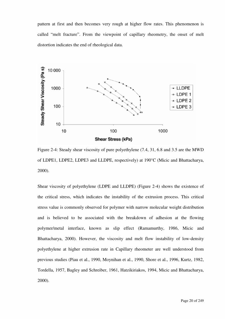
Page 20 of 249
pattern at first and then becomes very rough at higher flow rates. This phenomenon is
called “melt fracture”. From the viewpoint of capillary rheometry, the onset of melt
distortion indicates the end of rheological data.
Figure 2-4: Steady shear viscosity of pure polyethylene (7.4, 31, 6.8 and 3.5 are the MWD
of LDPE1, LDPE2, LDPE3 and LLDPE, respectively) at 190°C (Micic and Bhattacharya,
2000).
Shear viscosity of polyethylene (LDPE and LLDPE) (Figure 2-4) shows the existence of
the critical stress, which indicates the instability of the extrusion process. This critical
stress value is commonly observed for polymer with narrow molecular weight distribution
and is believed to be associated with the breakdown of adhesion at the flowing
polymer/metal interface, known as slip effect (Ramamurthy, 1986, Micic and
Bhattacharya, 2000). However, the viscosity and melt flow instability of low-density
polyethylene at higher extrusion rate in Capillary rheometer are well understood from
previous studies (Piau et al., 1990, Moynihan et al., 1990, Shore et al., 1996, Kurtz, 1982,
Tordella, 1957, Bagley and Schreiber, 1961, Hatzikiriakos, 1994, Micic and Bhattacharya,
2000).
Page 21 of 249
In this study, data obtained from both parallel plate rotational rheometer (Advanced
Rheometric Expansion System (ARES)) and Capillary rheometer have been combined to
determine the steady shear rheology and melt flow curve of the LDPEs.
2.2.2 Extensional rheology
Solidification of the polymer melts in industrial operations frequently involves stretching
action before reaching ’frozen-in’ strains and stresses. This stretching and solidification
process has major effects on the properties of the final products (Prasad, 2004, Raible et
al., 1982). Extensional rheology is associated with the uniaxial, biaxial and planar
stretching of different polymer processing operations. The extensional component is
generally present wherever streamlines converge or diverge. Melt spinning and parison sag
in blow molding are example of uniaxial extension. The film blowing process is an
example of biaxial extension, while film casting invokes deformations in between uniaxial
and planar (Dealy and Wissburn, 1990). Extensional rheology is a useful technique to
determine the non-linear behaviour of the polymer melt in the film blowing process (Micic
et al., 1998). Therefore, it is necessary to pay extra attention to determine the extensional
rheology of the polymer melts to understand their processing behaviour. Based on
extensional properties, Ziabicki (1976) provided a fundamental review of various forms of
fibre spinning operations, their kinematics and molecular orientations of the polymer.
(Gramespacher and Meissner, 1997) discussed the elastic recovery of the sample following
maximum extension and related the recovery to the concentration of PS in PMMA matrix.
Drawability in the film blowing (biaxial extension) process is defined as the ability of a
melt to be stretched into a thin film without breaking and is associated with strain
softening. On the other hand, good bubble stability is associated with the strain hardening
(Dealy and Wissburn, 1990). Therefore, in the blown film process, extensional rheology is
Page 22 of 249
very important to determine the “drawability” of the melt and the blown film “bubble
stability”.
Baird (1999) reported that there are a number of situations when two polymers have
identical shear flow properties, but process differently due to their differences in the degree
of long chain branching. It is worthy to mention that the subtle changes in molecular
architecture due to several factors such as branching and the presence of a high molecular
weight tail in the distribution are readily detected in the processing performance of the
polymer which is not detected in the shear flow properties. Most of the melt processing
involves some kind of extensional flow such as converging flow, as in a die or nozzle
where there is a presence of uniaxial or planar extension depending on the flow geometry.
That is why in the last two to three decades the importance of extensional deformation has
become popular to determine the processibility of commercial polymers (Takahashi et al.,
1999, Cogswell, 1972, Raible et al., 1982, Dealy and Wissburn, 1990, Laun, 1978,
Haward, 1993, Samurkas et al., 1989).
2.2.2.1 Extensional (elongational) viscosity of polyethylene
Münstedt and Laun (1981) reported an extensive study of extensional flow of LDPE and
their dependency on the molecular structure. In their study, three different LDPEs of
different MWD (7.0, 8.2 and 24.2 for LDPE1, LDPE2, LDPE3, respectively) and quite
similar densities and degrees of long chain branching were considered (Figure 2-5). They
observed a significant effect of high molecular weight tail of LDPE3 on the extensional
viscosity. They also reported that strain hardening behaviour of LDPEs with constant Mw
increases with their degree of long chain branching while their zero shear viscosity was
found to decrease. Micic and Bhattacharya (2000) reported similar effect of long chain
branching of LDPEs on the extensional viscosity. Therefore, it is essential to understand

Page 23 of 249
the effect of molecular structure (Mw, MWD and LCB) of LDPE on melt extensional
viscosity of the polymer before they are chosen to process.
Figure 2-5: Extensional viscosity versus tensile stress of three different LDPEs (Dealy and
Wissburn, 1990).
Simple extension that has been carried out mostly in the experimental rheology is the
uniaxial extension, which is an axisymmetric flow with stretching in the direction of the
axis of symmetry. In extensional rheology, strain hardening of the materials is a related
issue to determine their processability in the field of stretching. If the stress increases more
rapidly than would be predicted by the linear theory, the material is said to be” strain
hardening” (Figure 2-6). Usually polymers with a higher degree of long chain branching
show more strain hardening in comparison to the polymers with short or no branching
(Micic et al., 1998).

Page 24 of 249
Figure 2-6: Extensional viscosity of LDPE at different strain rates at 150°C (Münstedt et
al., 1998).
2.2.2.2 Uniaxial extensional test
Uniaxial extensional test is the most appropriate method to achieve maximum possible
strain hardening characteristics of the polymer melts (Laun and Schuch, 1989).
Determination of the melt extensional viscosity at high temperature is quite difficult due to
the sticking of low viscous melt with the experimental device. For the determination of
extensional rheology, the commonly used methods are (Cogswell, 1972):
• Constant stress measurements that involves sample end separation (Cogswell,
1969) or constant gauge length (improvisation of Meissner type equipment)
(Meissner, 1972)
• Constant strain rate measurements that involve sample end separation (Ballman,
1965) or constant (Meissner, 1972).
• Continuous drawing experiments(e.g., drawing of an extruded monofilament)

Page 25 of 249
Although there are several techniques available for measuring extensional flow properties,
the Meissner type rheometer will be used in this study. This instrument has been used
previously in this Rheology and Materials Processing Centre to measure the extensional
properties of various unfilled and filled polymer melts (Ivanov et al., 2004, Muke et al.,
2001, Prasad, 2004, Pasanovic-Zujo et al., 2004).
2.2.2.2.1 Meissner-type rheometer
This constant strain rate rheometer was developed by Meissner (1972) and since then
modifications were made to overcome the various associated problems (Meissner and
Hostettler, 1994, Meissner, 1995). Details of the instrument and its use have been provided
by Meissner and Hostettler (1994). A schematic diagram of the working principle is shown
in Figure 2-7. Extensional measurements are conducted isothermally. In this instrument, a
rod or rectangular shaped sample of length, L0 is held between two sets of rotary clamps,
C1 and C2. The sample is floated on a suitable fluid (silicone oil or nitrogen or air) to
reduce gravitational effects. The rotary clamps continuously convey the polymer that is
within the clamps outside, thus maintaining the basis length, L0. This action prevents
necking of stretched sample near the clamps and preserving a homogeneous cross section
during deformation (Meissner et al., 1981).
Figure 2-7: Schematic diagram of uniaxial stretching using the Meissner-type extensional
rheometer.
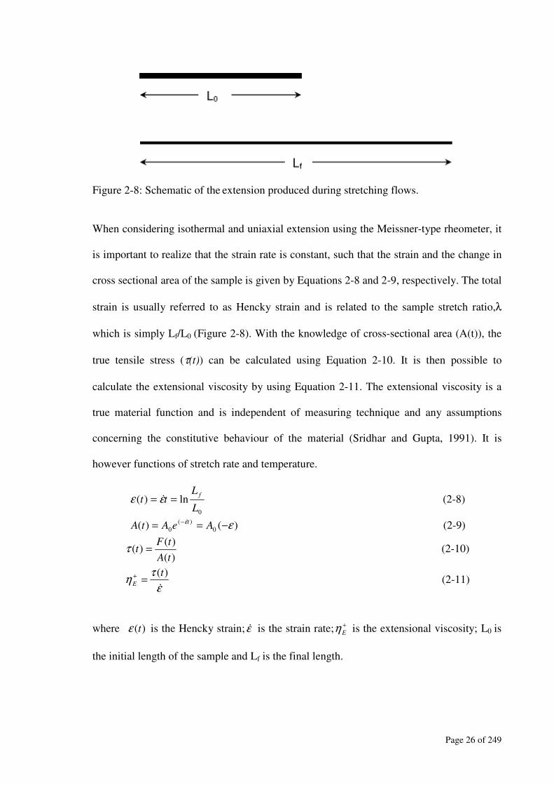
Page 26 of 249
Figure 2-8: Schematic of the extension produced during stretching flows.
When considering isothermal and uniaxial extension using the Meissner-type rheometer, it
is important to realize that the strain rate is constant, such that the strain and the change in
cross sectional area of the sample is given by Equations 2-8 and 2-9, respectively. The total
strain is usually referred to as Hencky strain and is related to the sample stretch ratio,λ
which is simply Lf/L0 (Figure 2-8). With the knowledge of cross-sectional area (A(t)), the
true tensile stress (τ(t)) can be calculated using Equation 2-10. It is then possible to
calculate the extensional viscosity by using Equation 2-11. The extensional viscosity is a
true material function and is independent of measuring technique and any assumptions
concerning the constitutive behaviour of the material (Sridhar and Gupta, 1991). It is
however functions of stretch rate and temperature.
0
ln)(L
Ltt
f
== εε ɺ (2-8)
)()( 0
)(
0 εε −== −AeAtA
tɺ (2-9)
)(
)()(
tA
tFt =τ (2-10)
ε
τη
ɺ
)(tE
=+ (2-11)
where )(tε is the Hencky strain;εɺ is the strain rate; +E
η is the extensional viscosity; L0 is
the initial length of the sample and Lf is the final length.

Page 27 of 249
The main material parameter that is often studied using this extensional apparatus is the
transient extensional viscosity, strain hardening characteristics or tensile stress growth at
constant strain rates (Yamaguchi and Suzuki, 2002). Wagner et al (2000) generalized the
Doi-Edwards model to the molecular stress function theory to quantitatively describe
extensional viscosities of polyolefin melts in constant strain rate extensional flow
experiments. The enhanced strain hardening in extensional flow was quantified using the
molecular stress function. All the extensional experiments were conducted using the
Meissner-type rheometer.
2.2.3 Effect of branching on melt rheology
The degree of branching, mainly the long chain branching (LCB) of LDPE has a
significant effect on the zero shear viscosity, temperature dependency on viscosity,
extensional viscosity, extruder performance and blown film strength properties (Dealy and
Wissburn, 1990). Many polymers have branches whose lengths are higher than critical
length required for entanglements like a linear chain. This sort of branches strongly
influences the melt rheology in both the shear and extensional field. The effect of long
chain branching (LCB) of LDPE on zero shear viscosity have been studied by several
researchers (Allen and Fox, 1964, Tung, 1960, Busse and Longworth, 1962, Long et al.,
1964, Mendelson et al., 1970, Micic and Bhattacharya, 2000). In those studies, it has been
conflictingly reported that branched polymers always have lower ZSV than their linear
analogy of the same molecular weight and at higher molecular weight, although the
branched polymers may have higher ZSV than the linear analogs. Dealy and Wissburn
(1990) mentioned that branched polymers with low molecular weights (Mw) and low
branch lengths show lower ZSV than that of linear polymer of the same Mw and this
resulted from the smaller coil radius of the polymer chains. Long branches reduce the
radius of gyration of a branched polymer in comparison to a linear chain of same
Page 28 of 249
molecular weight. Therefore decreased radius of gyration results in fewer entanglements
and a lower viscosity.
For commercial polymer, branching is usually accompanied by broadening the MWD
which increases both shear and extensional sensitivity (Dealy and Wissburn, 1990). Length
of the branch is equally important along with the number of branches to describe the melt
rheology. Therefore, it is really difficult to differentiate the effects of branching and
molecular weight distribution (MWD) due to a probability of broadening the MWD when
branching is occurred (Minoshima and White, 1984). When the branch length is
sufficiently long and higher than the critical molecular weight required for entanglement,
the overall entanglement network has a much longer lifetime than that of a linear polymer
network (Dealy and Wissburn, 1990). The higher degree of LCB enhances the
entanglement efficiency of the polymer molecules. Due to the effect of higher degree of
LCB of LDPE, ZSV increases and breadth of viscoelastic relaxation spectrum extends into
much longer relaxation times (Wood-Adams et al., 2000). Münstedt and Laun (1981) also
reported that zero shear viscosity increases much more steeply with Mw than the 3.4 power
relationship for LDPEs with higher degree of long chain branching.
Long chain branched polymers also show higher shear thinning and activation energy for
viscosity in comparison to the linear polymers of the same molecular weight. The flow
activation energy varies from about 54 kJ/mol for the linear polymer to about 116 kJ/mol
for branched polymer (Dealy and Wissburn, 1990). Macosko (1994) mentioned the change
of flow activation energy from about 25kJ/mol for polyethylene to 60kJ/mol for
polystyrene. Dependency of viscosity on temperature is higher for polymer having higher
flow activation energy (Dealy and Wissburn, 1990).

Page 29 of 249
2.3 Wide angle X-ray scattering (WAXD)
WAXD is one of the predominant forms of characterization techniques to understand the
molecular structure of the polymer material using the peak intensities and their width with
respect to the diffraction angle. It offers a convenient and rapid method for structural
characterization, for instance the interlayer spacing of the molecules (Vaia and Lincoln,
2002). The basic principle of WAXD is shown in Figure 2-9. Cullity (1978) pointed out
the importance of XRD to recognize two factors:
• Incident beam, normal to the reflecting plane and diffracted or scattered beam are
coplanar and
• The angle between the incident and scattered beam is always 2θ. This angle is
known as the scattering angle.
Figure 2-9: Schematic of X-Ray diffraction
The spacing between the ordered arrays of atoms is typically analysed using X-Ray
diffraction (Figure 2-9). It is the desired means of measuring lamella thickness, or long
spacing according to Bragg’s law of optics (Equation 2-12)
θ
λ
sin2
nd = (2-12)
where n = Diffraction order = 1 (first order for most commercial applications)
λ = Wave length (for Cu-Kα radiation wave length = 1.54Å)
d = Spacing between atomic planes
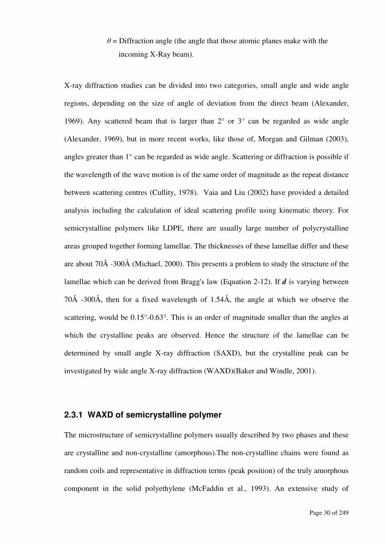
Page 30 of 249
θ = Diffraction angle (the angle that those atomic planes make with the
incoming X-Ray beam).
X-ray diffraction studies can be divided into two categories, small angle and wide angle
regions, depending on the size of angle of deviation from the direct beam (Alexander,
1969). Any scattered beam that is larger than 2° or 3° can be regarded as wide angle
(Alexander, 1969), but in more recent works, like those of, Morgan and Gilman (2003),
angles greater than 1° can be regarded as wide angle. Scattering or diffraction is possible if
the wavelength of the wave motion is of the same order of magnitude as the repeat distance
between scattering centres (Cullity, 1978). Vaia and Liu (2002) have provided a detailed
analysis including the calculation of ideal scattering profile using kinematic theory. For
semicrystalline polymers like LDPE, there are usually large number of polycrystalline
areas grouped together forming lamellae. The thicknesses of these lamellae differ and these
are about 70Å -300Å (Michael, 2000). This presents a problem to study the structure of the
lamellae which can be derived from Bragg's law (Equation 2-12). If d is varying between
70Å -300Å, then for a fixed wavelength of 1.54Å, the angle at which we observe the
scattering, would be 0.15°-0.63°. This is an order of magnitude smaller than the angles at
which the crystalline peaks are observed. Hence the structure of the lamellae can be
determined by small angle X-ray diffraction (SAXD), but the crystalline peak can be
investigated by wide angle X-ray diffraction (WAXD)(Baker and Windle, 2001).
2.3.1 WAXD of semicrystalline polymer
The microstructure of semicrystalline polymers usually described by two phases and these
are crystalline and non-crystalline (amorphous).The non-crystalline chains were found as
random coils and representative in diffraction terms (peak position) of the truly amorphous
component in the solid polyethylene (McFaddin et al., 1993). An extensive study of
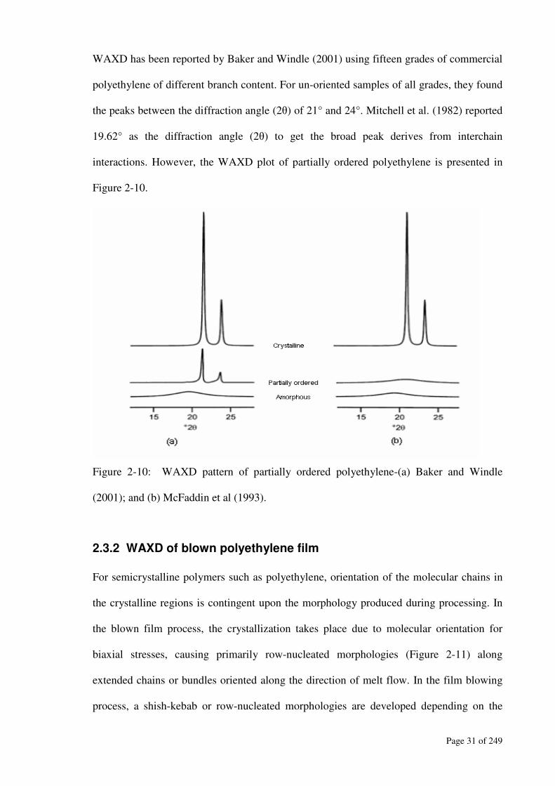
Page 31 of 249
WAXD has been reported by Baker and Windle (2001) using fifteen grades of commercial
polyethylene of different branch content. For un-oriented samples of all grades, they found
the peaks between the diffraction angle (2θ) of 21° and 24°. Mitchell et al. (1982) reported
19.62° as the diffraction angle (2θ) to get the broad peak derives from interchain
interactions. However, the WAXD plot of partially ordered polyethylene is presented in
Figure 2-10.
Figure 2-10: WAXD pattern of partially ordered polyethylene-(a) Baker and Windle
(2001); and (b) McFaddin et al (1993).
2.3.2 WAXD of blown polyethylene film
For semicrystalline polymers such as polyethylene, orientation of the molecular chains in
the crystalline regions is contingent upon the morphology produced during processing. In
the blown film process, the crystallization takes place due to molecular orientation for
biaxial stresses, causing primarily row-nucleated morphologies (Figure 2-11) along
extended chains or bundles oriented along the direction of melt flow. In the film blowing
process, a shish-kebab or row-nucleated morphologies are developed depending on the
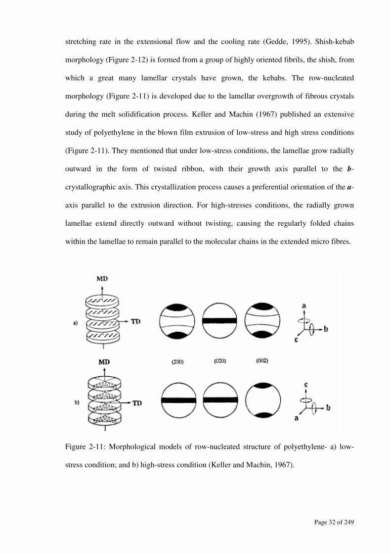
Page 32 of 249
stretching rate in the extensional flow and the cooling rate (Gedde, 1995). Shish-kebab
morphology (Figure 2-12) is formed from a group of highly oriented fibrils, the shish, from
which a great many lamellar crystals have grown, the kebabs. The row-nucleated
morphology (Figure 2-11) is developed due to the lamellar overgrowth of fibrous crystals
during the melt solidification process. Keller and Machin (1967) published an extensive
study of polyethylene in the blown film extrusion of low-stress and high stress conditions
(Figure 2-11). They mentioned that under low-stress conditions, the lamellae grow radially
outward in the form of twisted ribbon, with their growth axis parallel to the b-
crystallographic axis. This crystallization process causes a preferential orientation of the a-
axis parallel to the extrusion direction. For high-stresses conditions, the radially grown
lamellae extend directly outward without twisting, causing the regularly folded chains
within the lamellae to remain parallel to the molecular chains in the extended micro fibres.
Figure 2-11: Morphological models of row-nucleated structure of polyethylene- a) low-
stress condition; and b) high-stress condition (Keller and Machin, 1967).
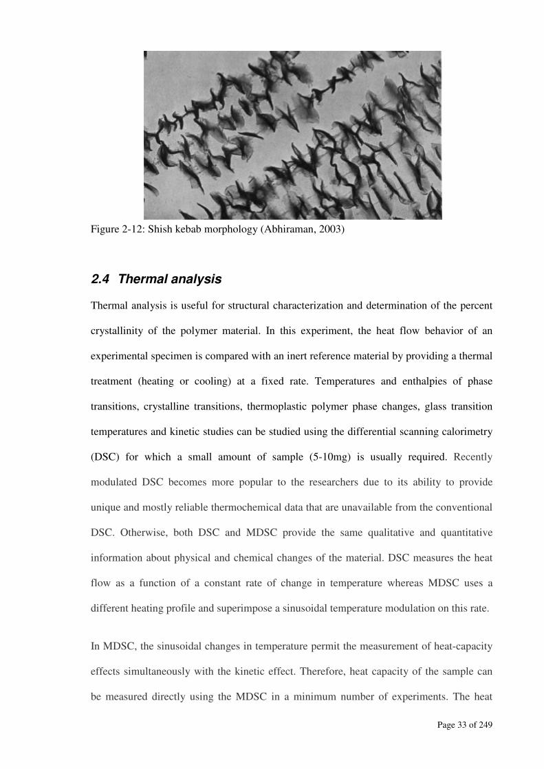
Page 33 of 249
Figure 2-12: Shish kebab morphology (Abhiraman, 2003)
2.4 Thermal analysis
Thermal analysis is useful for structural characterization and determination of the percent
crystallinity of the polymer material. In this experiment, the heat flow behavior of an
experimental specimen is compared with an inert reference material by providing a thermal
treatment (heating or cooling) at a fixed rate. Temperatures and enthalpies of phase
transitions, crystalline transitions, thermoplastic polymer phase changes, glass transition
temperatures and kinetic studies can be studied using the differential scanning calorimetry
(DSC) for which a small amount of sample (5-10mg) is usually required. Recently
modulated DSC becomes more popular to the researchers due to its ability to provide
unique and mostly reliable thermochemical data that are unavailable from the conventional
DSC. Otherwise, both DSC and MDSC provide the same qualitative and quantitative
information about physical and chemical changes of the material. DSC measures the heat
flow as a function of a constant rate of change in temperature whereas MDSC uses a
different heating profile and superimpose a sinusoidal temperature modulation on this rate.
In MDSC, the sinusoidal changes in temperature permit the measurement of heat-capacity
effects simultaneously with the kinetic effect. Therefore, heat capacity of the sample can
be measured directly using the MDSC in a minimum number of experiments. The heat
Page 34 of 249
capacities calculated from the modulated response to the variable temperature depend on
the frequency for a given cell constant (Cser et al., 1997). The linear dependence of
temperature on time is modulated by a periodical function. The modulation can be
sinusoidal, saw-tooth or a periodical alteration of heating-isotherm.
The principle of the method can be explained for the sinusoidal modulation, the
dependence of temperature on time can be expressed as (Chaudhary, 2004):
tytTT ωβ sin0 ++= (2-13)
where y is the amplitude and ω is the angular speed of modulation.
The signals registered by the apparatus can be divided into two kinds:
(i) Signal dependent on the rate of temperature change connected mainly with the
heat capacity of the sample.
(ii) Signal dependent on the absolute value of temperature connected mainly with
the kinetics of physical and chemical transformations.
The overall signal represents an overlap of both the signals (Chaudhary, 2004):
),( Ttfdt
dTcP
p+= (2-14)
where f is the function describing the kinetics of the transformation. If the sinusoidal
modulation is considered a perturbation, then the influence of the modulation can be
expressed by a Taylor series. Combination of the previous equations (Equations 2-13 and
2-14) gives:
tCTtftycPp
ωωωβ sin),()cos(0 +++= (2-15)
where 0f is the kinetics without the temperature modulation and C is the amplitude of
kinetic response. The equipment records the actual (modulated) temperature, the
instantaneous (modulated) heat flow in response to the temperature function and phase
Page 35 of 249
angle of two harmonic functions. The signal is treated by the Fourier analysis to determine
the response of the temperature function. The cosine component is connected with the
thermodynamically reversible effects of heat capacity. This component is thus called
reversible. The sine component is connected with the thermodynamically irreversible
kinetic effects and is called irreversible. According to Cser et al (1997), the heat flow in
MDSC can be divided into two parts (Equation 2-16):
kineticreversibletotaldt
dQ
dt
dQ
dt
dQ
+
=
(2-16)
2.4.1 Thermal analysis of polyethylene
The content of the crystalline component in semicrystalline polymers such as LDPE or
HDPE (high-density polyethylene) is a major factor affecting the mechanical, physical and
optical properties of the final product. The melting of polymer crystals exhibits many
instructive features of non-equilibrium behavior. Previously a lot of works studied the
MDSC to determine the melting and crystalline properties of the semicrystalline polymer
such as LDPE and HDPE (Gill et al., 1993, Reading et al., 1993, Xie et al., 2003,
Chaudhary, 2004, Cser et al., 1997). Standard heat (to obtain 100% crystallinity) of 287.3
J/g was used to determine the percent crystallinity of the polyethylens and crystallinity was
found to vary between 39% to 50% (Xie et al., 2003). The percent crystallinity obtained
from the heat of fusion is based on the measurement of the area under the MDSC melting
peak. The choice of base line is crucial, particularly for polymers of low crystallinity. The
factors such as molecular weight, degree of branching and cooling rate have significant
influence on the crystal thickness and hence to the heat flow behavior and the melting
point (Gedde, 1995). A typical MDSC plot (heat flow versus temperature) of polyethylene
is presented in Figure 2-13 . Therefore, any variation in the heat flow curve or melting
point of the polyethylene under investigation will indicate their structural variations (e.g.,
molecular weight or degree of branching etc.).

Page 36 of 249
Figure 2-13: Thermograms (heating cycle) of three different polyethylene.
2.5 Blown film properties
Study of the structure of polyethylene blown film has been going on for the last few
decades, but a good understanding of the structural features and their relationship to
physical behaviors is still lacking. It has been revealed that molecular orientations of the
blown film are significantly affected by the molecular structure (e.g., Mw and LCB) and
rheology of the processed polymers along with the processing parameters such as die
temperature, cooling rate, blow up ratio (BUR) and draw down ratio (DDR) (Godshall et
al., 2003, Patel et al., 1993, Zhang et al., 2004). Polymer with narrow MWD and modest
degree of branching will provide good drawability and optical properties, but this
combination of characteristics won’t give better impact strength (Dealy and Wissburn,
1990), which is an important film properties for flexible packaging. It is also reported in
the literature that at identical film blowing conditions, resins with longer characteristic
Page 37 of 249
melt relaxation times show a greater degree of lamellar stacking, increased level of
molecular orientation (Sukhadia, 1998), which have a significant effect on the film
properties. The film properties, which are maintained consistent for the most packaging
(flexible or non-flexible) applications are:
• Mechanical properties(Tear, Tensile and Impact strength)
• Optical properties(Gloss and Haze)
• Shrinkage properties
LDPE with higher degree of LCB leaves highly oriented fibrillar nuclei to promote the row
structure over the spherulites, which has a significant effect on the film properties (Wood-
Adams et al., 2000). Fruitwala et al (1995) and Maddams and Preedy (1978) studied with
high Mw-high density polyethylene (HDPE) and linear low-density polyethylene (LLDPE)
and concluded a correlation of machine direction tear strength with their molecular
properties and their orientation. Dormier et al (1989) studied the blown film using TEM
and small angle X-Ray scattering (SAXS) along with bubble kinematics to determine the
structure-property relationships. Based on their study, it has been revealed that identical
resins (as measured by GPC and dynamic rheological characteristics) may provide
significantly different physical and morphological properties. They reported that long
chain branching (LCB), MWD, rheology (both shear and extensional) and film dynamics
are responsible for the complex interdependence of polymer structure, solid state structure
and solid state film properties (Sukhadia et al., 2002, Lu et al., 2000, Lu and Sue, 2002,
Sukhadia, 1998, Patel et al., 1993, Zhang et al., 2004).

Page 38 of 249
2.5.1 Mechanical properties
2.5.1.1 Tensile strength
Tensile strength of the film determines the maximum amount of resisting stress to pull the
molecules apart or break. The value of the tensile strength is usually obtained by dividing
the maximum load observed during tensile straining by the specimen cross-sectional area
before it breaks. Tensile strength depends on the nature of the polymer backbone. The
steps during the tensile testing are: (i) elongation of the tie chains between the lamellae
structure; (ii) tilting of lamellar structure towards the tensile axis; (iii) separation of the
crystalline blocks; and (iv) stretching of crystalline and amorphous blocks in a fibrillar
structure along the axis of tension.
LDPE generally has a higher melt entanglement and strain hardening during melt
elongation due to the presence of LCB. The degree of LCB in the order of 1-3 per 1000
carbon atoms in the LDPE will show low tensile strength and modulus and medium impact
and tear resistance (Zhang et al., 2004). According to the processing-structure-property
relationship study of LDPE (Patel et al., 1993), it is reported that tensile strength in MD is
higher due to the higher values of tie molecules in the amorphous orientation along MD.
Study of the morphology and orientation (Figure 2-14) of LDPE reported the anisotropic
behaviour of tensile properties, which are related to the formation of fibrillar structure
(Zhang et al., 2004).

Page 39 of 249
Figure 2-14: Schematic of morphological developments and structure-tear relationship of
polyethylene (Zhang et al., 2004).
2.5.1.2 Tear strength
Tear strength determines the energy necessary to propagate a tear in the film. In the tearing
process, the predominant mechanism is the breaking of chains. The surfaces of the tear
cracks are rough on a molecular scale since the tear follows a path of least resistance to
minimize the number of chains that are broken. It is well known that a high degree of
chain orientation along MD leads to poor tear resistance in MD. Those films, which have
the higher degree of MD orientation, have enhanced tear strength along TD.
Tear anisotropy in polyethylene blown films were studied by Lee et al (2005) and found
that linear molecules of high Mw are able to extend in response to the extensional flow
during film blowing and thus form tie molecules more readily and show higher resistance
in tearing along TD. Highly branched molecules such as LDPE are less able to align in
Page 40 of 249
MD, which allows the lamellae to be separated and shows almost lower value of tear
resistance along TD (Zhang et al., 2004). A metallocene catalysed ethylene-hexane
copolymer with its narrow molecular weight distribution, relaxes quickly after extension
and produces films of isotropic tear strength (Lee et al., 2005, Zhang et al., 2004).
Patel et al (1993) reported that tear in MD for a given resin is governed by the extension
and the orientation of molecules in the amorphous phase. Godshall et al (2003) studied
two different HDPE and reported that tear properties (according to ASTM D1922) are a
strong function of molecular anisotropy and thicker films produce greater tear strength as
expected due to the greater amount of material being tested. Adjustment of the freeze line
height by changing the cooling rates may improve chain orientation in both direction (MD
and TD) and hence the tear strength (Godshall et al., 2003, Patel et al., 1993).
2.5.1.3 Impact strength
Impact strength determines the energy to fracture a film and to characterize film behaviour
under high loading. For blown film, dart impact strength depends on the die gap and the
BUR. Higher BUR would lead to more balanced orientation as well as to a higher degree
of planar orientation and thus increasing the dart impact. Depending on the type of
material, narrow die gap may influence melt fracture and hence surface roughness in the
film.
Firdaus and Tong (1992) reported that melt fracture strongly influences the impact
strength and rougher films are related to the lower values of dart impact strength. In
contrast, it is also found in the literature (Ealer et al., 1991) that impact strength of LLDPE
or VLDPE (0.91 gm/cc) decreases with an increase in die gap and MD tear strength and
dart impact were reported to increase as the level of MD orientation decreases. Godshall

Page 41 of 249
et al (2003) demonstrated that impact strength is not dependent on the film thickness and it
is higher at lower cooling rates (higher FLH) due to more balanced orientation in both
direction (MD and TD). Patel et al (1993) reported for LLDPE films that higher BUR and
die gap are suitable to get better dart impact strength due to more amorphous orientation
and absence of surface roughness. They also found that at any die gap the dart impact
strength decreases with the MD shrinkage.
2.5.2 Optical (haze and gloss) properties
Haze is the percentage of transmitted light, passed through the specimen but deviating
from the incident beam by forward scattering. According to the standard (ASTM-D1003),
the light flux deviating more than 2.5° is considered to be haze.
Gloss is the ratio of the luminous flux reflected from a specimen to a standard surface
under the same geometric conditions. Haze due to surface roughness is in many cases
inversely related to gloss. Optical properties of the LDPE films can vary substantially
depending on the extent of light which is scattered by the irregularities of the film surface.
It is reported earlier that surface irregularities are responsible for haze properties of the
polyethylene film (Huck and Clegg, 1961, Clegg and Huck, 1961, Sukhadia et al., 2001,
Clampitt et al., 1969, Stehling et al., 1981). In the film blowing process, the rough surfaces
are formed by two mechanisms, one involving melt flow disturbances at the die exit,
known as “extrusion defects” and the other caused by stress-induced crystallization close
to the film surface (Stehling et al., 1981). The crystallinity has a great influence to surface
texture. As the extruded melt solidifies, crystal lamellae protrude from the film surface,
thereby giving rise to surface roughness. This type of surface irregularities are knows as
“crystallization defects” (Pucci and Shroff, 1986). Surface roughness due to melt flow-
Page 42 of 249
induced phenomena occurs as a consequence of the polymer melt elasticity (Clegg and
Huck, 1961, Pucci and Shroff, 1986).
Melt elasticity can be used as a useful indicator for blown film optical properties. For HP-
LDPE, it is reported earlier that lower value of blown film haze properties are related to
their lower value of melt elasticity (Fujiki, 1971, Pucci and Shroff, 1986). In contrast
Cooke and Tikuisis (1989) reported haze properties of LLDPE film to improve(decrease)
with the increase of melt elasticity. Dealy and Wissburn (1990) mentioned that polymer
with narrow molecular weight distribution and modest degree of branching will provide
good optical properties. Therefore, when the resins are processed at identical conditions,
optical properties of the film will be different due to their different molecular structure
(molecular weight and its distribution and degree of branching).
2.5.3 Shrinkage properties
Thermal shrinkage is the measure of chain extension in the amorphous phase (Lu and Sue,
2002) . This is considered to happen mainly due to the relaxation of extended and oriented
tie chains locked in by crystallites (Liu and Harrison, 1988).
The shrinkage is dependent on the molecular properties (e.g. length of the chain and type
of branching) of the polymer, shrinking time and temperature and thickness of the film.
The shrinking temperature is usually selected between glass transition temperature (Tg) and
melting point(Tm) or above Tm, depending on the polymer system. In various shrinkage
testing, changes in dimensions of the sample (Pinnock and Ward, 1964, Ward, 1984), the
shrinkage rate (Kato and Yanagihara, 1981) and shrinkage stress (Henrici-Olive et al.,
1986) are determined. For LDPE, it is reported that at constant temperature, shrinking
Page 43 of 249
increases with time and at a constant time, shrinking increases with increased temperature
(Liu and Harrison, 1988).
The tie chains between crystalline lamellae account for a large portion of the amorphous
material. Therefore, the orientation of crystallites might have a large effect on the
amorphous phase orientation. During the blown film extrusion of LDPE, chain
entanglements are acting as physical crosslinks, which are extended and oriented during
biaxial stretching and crystallized due to the effect of cooling. When the film is heated
above its melting point, chain segmental motion will again become activated. Extended
chain will try to return to a random coil and the net result will be the shrinking of the film
if no chain slippage occurs (Liu and Harrison, 1988). Therefore, shrinking of the blown
film will vary depending on the molecular structure of the polymer along with their
processing variables.
2.6 Summary
Based on the previous studies, it can be concluded that molecular, rheological and
crystalline properties have a significant effect on the blown film processability and film
properties (mechanical and optical) during extrusion of the polymer.
Molecular properties of the commercial grades of LDPE vary from one manufacturer to
another and hence their melt rheology, crystallinity and morphology will also be different
than those published in the literature. To determine the processability and film properties
of a particular polymer, it is necessary to experiment them for analysis or other studies,
rather than referring to published data in the literature.
Page 44 of 249
A unique research for a film blowing process comprising numerical modelling and
simulation and its experimental verification will provide most useful and significant
information to the plastic film industry to optimise the process variables and film
properties. This study focused on experimental measurements using two different
commercial grades of LDPE to process them in the blown pilot plant and to determine their
rheological properties, process characteristics, film properties and crystallinity.
Although extensive studies of LDPE in blown film extrusion have been carried out in the
last few decades, effect of long chain branching (LCB) on blown film crystallinity has not
been reported. In addition, long chain property of LDPE and its effect on thermal and
rheological properties have not been described adequately in the literature. This research
also focused on those issues.
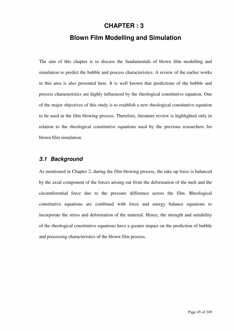
Page 45 of 249
CHAPTER : 3
Blown Film Modelling and Simulation
The aim of this chapter is to discuss the fundamentals of blown film modelling and
simulation to predict the bubble and process characteristics. A review of the earlier works
in this area is also presented here. It is well known that predictions of the bubble and
process characteristics are highly influenced by the rheological constitutive equation. One
of the major objectives of this study is to establish a new rheological constitutive equation
to be used in the film blowing process. Therefore, literature review is highlighted only in
relation to the rheological constitutive equations used by the previous researchers for
blown film simulation.
3.1 Background
As mentioned in Chapter 2, during the film blowing process, the take up force is balanced
by the axial component of the forces arising out from the deformation of the melt and the
circumferential force due to the pressure difference across the film. Rheological
constitutive equations are combined with force and energy balance equations to
incorporate the stress and deformation of the material. Hence, the strength and suitability
of the rheological constitutive equations have a greater impact on the prediction of bubble
and processing characteristics of the blown film process.
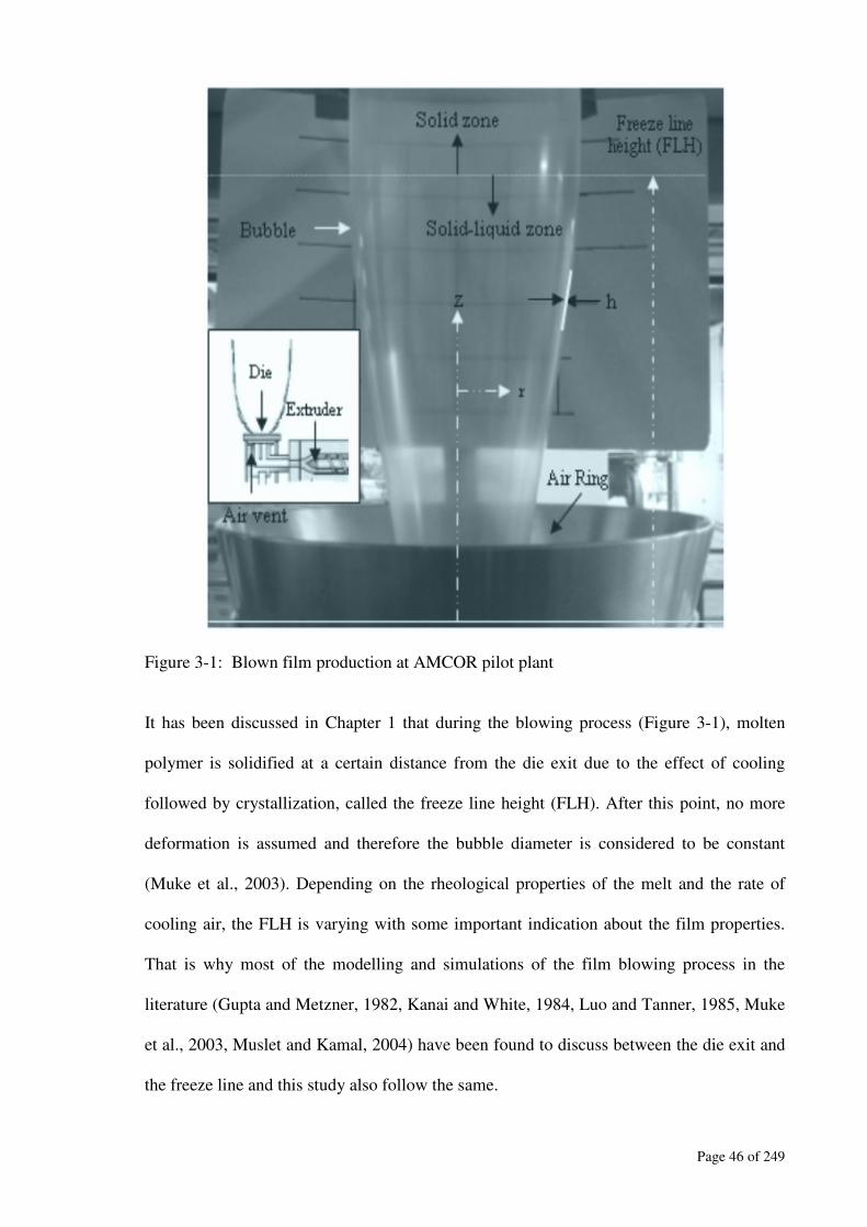
Page 46 of 249
Figure 3-1: Blown film production at AMCOR pilot plant
It has been discussed in Chapter 1 that during the blowing process (Figure 3-1), molten
polymer is solidified at a certain distance from the die exit due to the effect of cooling
followed by crystallization, called the freeze line height (FLH). After this point, no more
deformation is assumed and therefore the bubble diameter is considered to be constant
(Muke et al., 2003). Depending on the rheological properties of the melt and the rate of
cooling air, the FLH is varying with some important indication about the film properties.
That is why most of the modelling and simulations of the film blowing process in the
literature (Gupta and Metzner, 1982, Kanai and White, 1984, Luo and Tanner, 1985, Muke
et al., 2003, Muslet and Kamal, 2004) have been found to discuss between the die exit and
the freeze line and this study also follow the same.
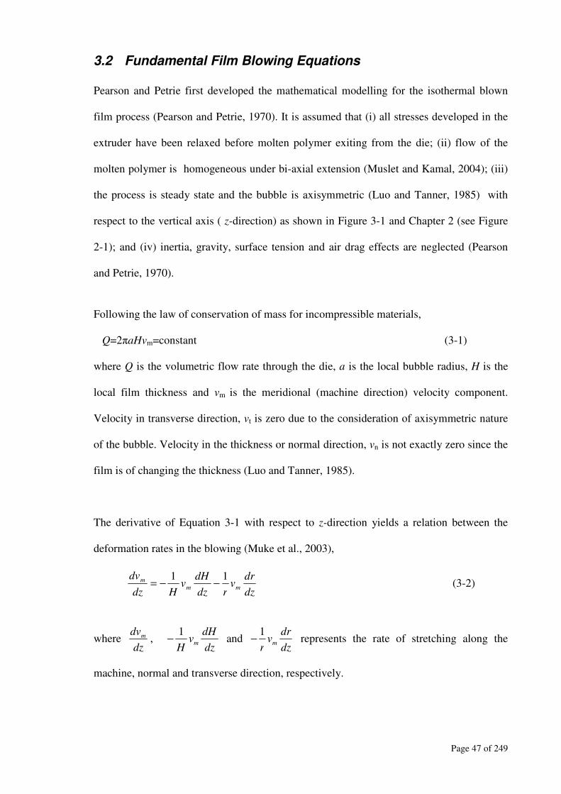
Page 47 of 249
3.2 Fundamental Film Blowing Equations
Pearson and Petrie first developed the mathematical modelling for the isothermal blown
film process (Pearson and Petrie, 1970). It is assumed that (i) all stresses developed in the
extruder have been relaxed before molten polymer exiting from the die; (ii) flow of the
molten polymer is homogeneous under bi-axial extension (Muslet and Kamal, 2004); (iii)
the process is steady state and the bubble is axisymmetric (Luo and Tanner, 1985) with
respect to the vertical axis ( z-direction) as shown in Figure 3-1 and Chapter 2 (see Figure
2-1); and (iv) inertia, gravity, surface tension and air drag effects are neglected (Pearson
and Petrie, 1970).
Following the law of conservation of mass for incompressible materials,
Q=2πaHvm=constant (3-1)
where Q is the volumetric flow rate through the die, a is the local bubble radius, H is the
local film thickness and vm is the meridional (machine direction) velocity component.
Velocity in transverse direction, vt is zero due to the consideration of axisymmetric nature
of the bubble. Velocity in the thickness or normal direction, vn is not exactly zero since the
film is of changing the thickness (Luo and Tanner, 1985).
The derivative of Equation 3-1 with respect to z-direction yields a relation between the
deformation rates in the blowing (Muke et al., 2003),
dz
drv
rdz
dHv
Hdz
dv
mm
m11
−−= (3-2)
where dz
dvm ,
dz
dHv
Hm
1− and
dz
drv
rm
1− represents the rate of stretching along the
machine, normal and transverse direction, respectively.
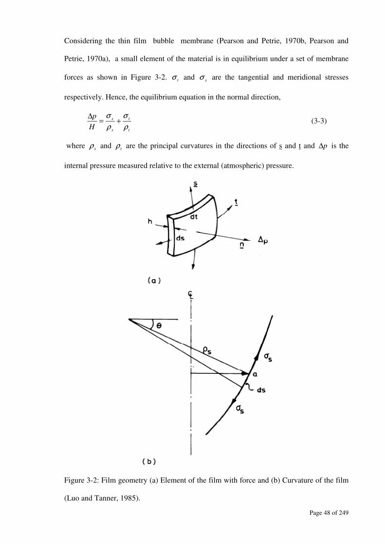
Page 48 of 249
Considering the thin film bubble membrane (Pearson and Petrie, 1970b, Pearson and
Petrie, 1970a), a small element of the material is in equilibrium under a set of membrane
forces as shown in Figure 3-2. t
σ and s
σ are the tangential and meridional stresses
respectively. Hence, the equilibrium equation in the normal direction,
t
t
s
s
H
p
ρ
σ
ρ
σ+=
∆ (3-3)
where s
ρ and t
ρ are the principal curvatures in the directions of s and t and p∆ is the
internal pressure measured relative to the external (atmospheric) pressure.
Figure 3-2: Film geometry (a) Element of the film with force and (b) Curvature of the film
(Luo and Tanner, 1985).
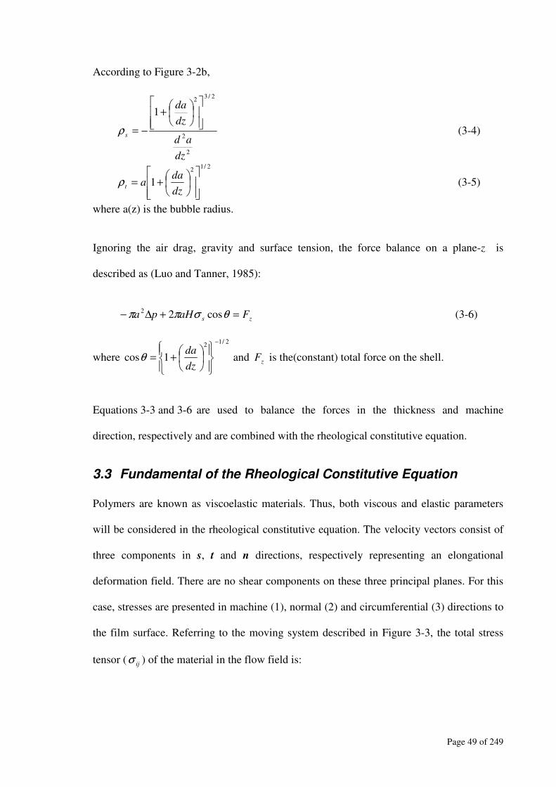
Page 49 of 249
According to Figure 3-2b,
2
2
2/32
1
dz
ad
dz
da
s
+
−=ρ (3-4)
2/12
1
+=
dz
daa
tρ (3-5)
where a(z) is the bubble radius.
Ignoring the air drag, gravity and surface tension, the force balance on a plane-z is
described as (Luo and Tanner, 1985):
zsFaHpa =+∆− θσππ cos22
(3-6)
where
2/12
1cos
−
+=
dz
daθ and
zF is the(constant) total force on the shell.
Equations 3-3 and 3-6 are used to balance the forces in the thickness and machine
direction, respectively and are combined with the rheological constitutive equation.
3.3 Fundamental of the Rheological Constitutive Equation
Polymers are known as viscoelastic materials. Thus, both viscous and elastic parameters
will be considered in the rheological constitutive equation. The velocity vectors consist of
three components in s, t and n directions, respectively representing an elongational
deformation field. There are no shear components on these three principal planes. For this
case, stresses are presented in machine (1), normal (2) and circumferential (3) directions to
the film surface. Referring to the moving system described in Figure 3-3, the total stress
tensor (ij
σ ) of the material in the flow field is:

Page 50 of 249
Figure 3-3: Coordinate systems describing the deformation of a bubble (Khonakdar et al.,
2002).
ijijijP τδσ +−= (3-7)
where p is the isotropic pressure, ij
τ is the deviatoric stresses ( some times it is known as
extra stress tensor) and ij
δ is the Kronecker delta:
≠
==
ji
ji
ij
0
1δ .
The success of the modelling relies mostly on the accurate calculation of deviatoric
stresses (ij
τ ) of the materials. To obtain both elastic and viscous properties of the
materials, it is necessary to define the deformation and rate of deformation of the material
during the blowing process.

Page 51 of 249
3.3.1 Deformations in the Film Blowing Process
The deformation of an element of fluid in the film blowing process (in each of the principal
directions) is defined as:
)ln()ln( 00
0
1rH
Hr
v
v==ε (3-8)
)ln(0
2H
H=ε (3-9)
)ln(0
3r
r=ε (3-10)
Considering v as the velocity vector and εɺ as the rate of deformation tensor,
=
3
3
2
2
1
1
00
00
00
δξ
δδξ
δδξ
δ
ε
v
v
v
ɺ (3-11)
Velocity in the machine direction is defined by:
dt
dv
1
1
ξ= (3-12)
2v is the velocity normal to the film thickness which is representative of the rate at which
the film is thinning. Since, h is a function of 1ξ , 2v can be defined by:
1
1
1
1
2ξ
ξ
ξ d
dhv
dt
d
d
dh
dt
dhv === (3-13)
The rate, at which the bubble expands, also known as the circumferential velocity, 3v is
defined as:
1
13 22ξ
ππd
dRv
dt
dRv == (3-14)
where R is bubble radius

Page 52 of 249
For a thin film, the gradient of velocity in the ξ2 direction ( 2εɺ ) (direction normal to the
film surface) is the difference in velocity ( 2v ) across the film thickness divided by the local
film thickness:
1
1
2
2
22v
d
dh
hh
v
ξε ==ɺ (3-15)
Since symmetry axis is assumed as the z-axis about which the bubble expands at a constant
rate, the stretching rate of deformation is the ratio of the increase of the circumference to
the local value of the circumference.
1
1
3
2
ξε
d
dR
R
v=ɺ (3-16)
Due to assumption of the incompressibility, the first invariant of the rate of deformation
tensor vanishes, hence:
+−=+−=
11
1321
112)(
ξξεεε
d
dR
Rd
dh
hvɺɺɺ (3-17)
The following relationships transform the change in the machine direction elemental
coordinate (ξ1) and the velocity in that direction ( 1v ).
dzdθ
ξcos
11 = (3-18)
Rh
Qv
π21 = (3-19)
Substituting Equations 3-18 and 3-19 into the rate of deformation tensor Equation
3-11 gives:
−−
=
dz
dR
R
dz
dh
h
dz
dR
Rdz
dh
h
Rh
Q
100
01
0
0011
cos
π
θεɺ (3-20)
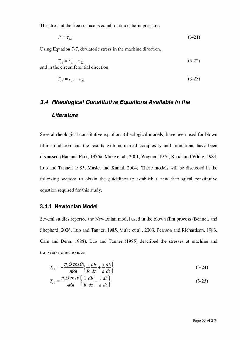
Page 53 of 249
The stress at the free surface is equal to atmospheric pressure:
22τ=P (3-21)
Using Equation 7-7, deviatoric stress in the machine direction,
221111 ττ −=T (3-22)
and in the circumferential direction,
223333 ττ −=T (3-23)
3.4 Rheological Constitutive Equations Available in the
Literature
Several rheological constitutive equations (rheological models) have been used for blown
film simulation and the results with numerical complexity and limitations have been
discussed (Han and Park, 1975a, Muke et al., 2001, Wagner, 1976, Kanai and White, 1984,
Luo and Tanner, 1985, Muslet and Kamal, 2004). These models will be discussed in the
following sections to obtain the guidelines to establish a new rheological constitutive
equation required for this study.
3.4.1 Newtonian Model
Several studies reported the Newtonian model used in the blown film process (Bennett and
Shepherd, 2006, Luo and Tanner, 1985, Muke et al., 2003, Pearson and Richardson, 1983,
Cain and Denn, 1988). Luo and Tanner (1985) described the stresses at machine and
transverse directions as:
+−=dz
dh
hdz
dR
RRh
QT
21cos0
11π
θη (3-24)
−=dz
dh
hdz
dR
RRh
QT
11cos0
33π
θη (3-25)
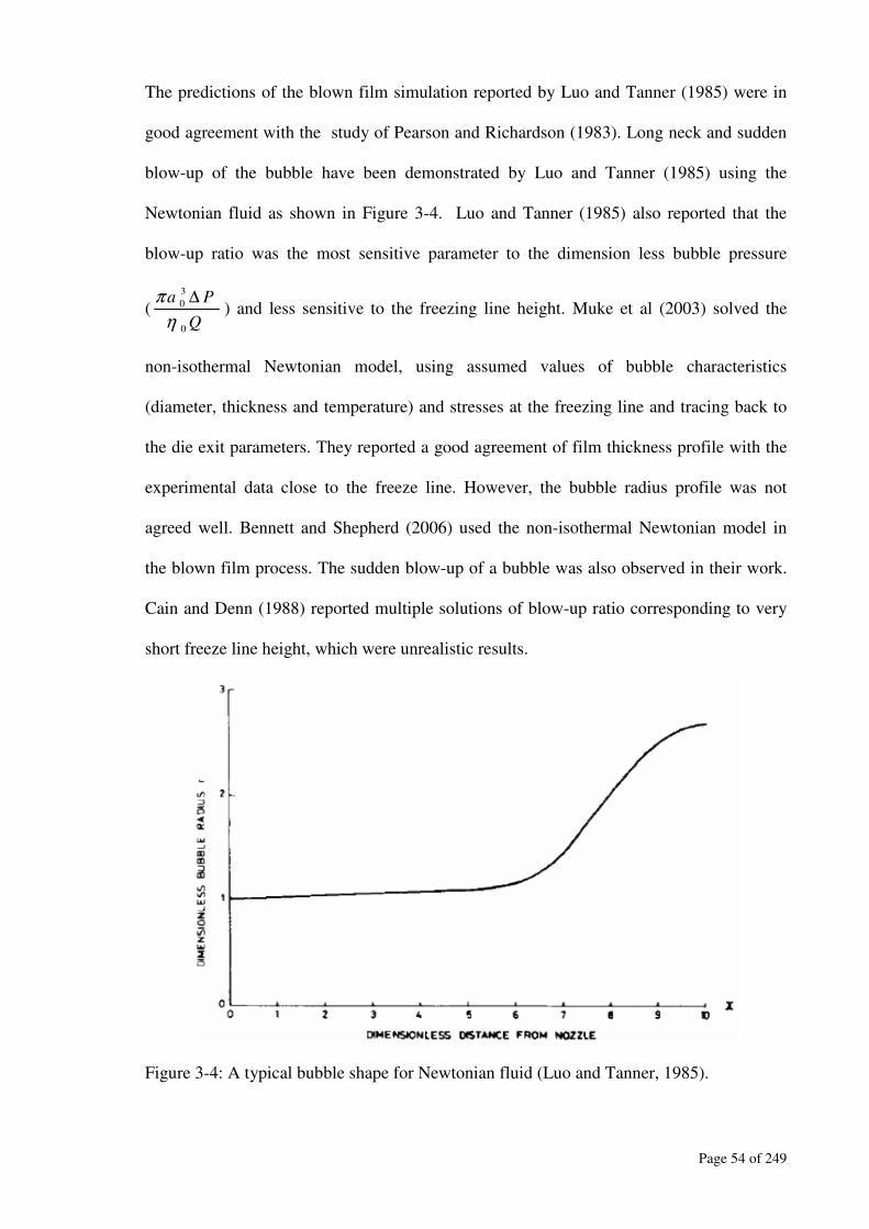
Page 54 of 249
The predictions of the blown film simulation reported by Luo and Tanner (1985) were in
good agreement with the study of Pearson and Richardson (1983). Long neck and sudden
blow-up of the bubble have been demonstrated by Luo and Tanner (1985) using the
Newtonian fluid as shown in Figure 3-4. Luo and Tanner (1985) also reported that the
blow-up ratio was the most sensitive parameter to the dimension less bubble pressure
(Q
Pa
0
3
0
η
π ∆) and less sensitive to the freezing line height. Muke et al (2003) solved the
non-isothermal Newtonian model, using assumed values of bubble characteristics
(diameter, thickness and temperature) and stresses at the freezing line and tracing back to
the die exit parameters. They reported a good agreement of film thickness profile with the
experimental data close to the freeze line. However, the bubble radius profile was not
agreed well. Bennett and Shepherd (2006) used the non-isothermal Newtonian model in
the blown film process. The sudden blow-up of a bubble was also observed in their work.
Cain and Denn (1988) reported multiple solutions of blow-up ratio corresponding to very
short freeze line height, which were unrealistic results.
Figure 3-4: A typical bubble shape for Newtonian fluid (Luo and Tanner, 1985).

Page 55 of 249
3.4.2 Power Law Model
An extensive study of uniaxial and biaxial extension process was reported by Han and
Park (Han and Park, 1975b, Han and Park, 1975a). Extensional viscosity of the polymer
melt was determined in the first part of their study (Han and Park, 1975b). Deformation of
the materials and heat transfer in the film blowing process were analysed in the second part
of their study (Han and Park, 1975a). They defined the total stress of the materials as:
ijijijPT τδ +−= (3-26)
( )ijBij
εητ ɺΠ= (3-27)
where ( )ΠB
η is the extensional viscosity and Π is the second invariant of the rate of
deformation tensor(.
ε ) expressed as:
2
33
2
22
2
11 εεε ɺɺɺ ++=Π (3-28)
Considering stresses in the machine and transverse directions (Equations 3-21 to 3-23, 3-
26, 3-27), they defined elongation viscosity in non-uniform bi-axial stretching as:
2211
11)(εε
ηɺɺ −
=ΠT
B (3-29)
or
2233
33)(εε
ηɺɺ −
=ΠT
B (3-30)
Using Equations 3-22 and 3-28 , the extensional rate defined for bi-axial stretching (Han
and Park, 1975b, Han and Park, 1975a) is:
2/122
1111
2
cos
2
+
+
=Π
dz
dh
hdz
dh
hdz
dR
Rdz
dR
RRh
Q
π
θ (3-31)
From the study of Han and Park (1975b), it can be found that extensional viscosities of
high-density polyethylene (HDPE) and polypropylene decrease with the extension rate,
whereas the extensional viscosity of low-density polyethylene increases with extension
rate as shown in Figures 3-5 to 3-7. Han and Park (1975b) also compared the extensional
viscosity determined from the blown film process and the melt-spinning process.
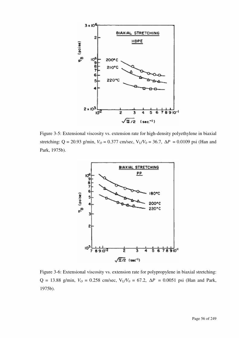
Page 56 of 249
Figure 3-5: Extensional viscosity vs. extension rate for high-density polyethylene in biaxial
stretching: Q = 20.93 g/min, VO = 0.377 cm/sec, VL/V0 = 36.7, P∆ = 0.0109 psi (Han and
Park, 1975b).
Figure 3-6: Extensional viscosity vs. extension rate for polypropylene in biaxial stretching:
Q = 13.88 g/min, VO = 0.258 cm/sec, VL/V0 = 67.2, P∆ = 0.0051 psi (Han and Park,
1975b).

Page 57 of 249
Figure 3-7: Extensional viscosity vs. extension rate for low-density polyethylene in biaxial
stretching: Q = 18.10 g/min, VO = 0.346 cm/sec, VL/V0 = 28.9, P∆ = 0.0058 psi (Han and
Park, 1975b).
Power law type of empirical expression was reported in the second part of the blown film
studies by Han and Park (1975a). Non-isothermal experiments were carried out in their
work to compare the model predictions. Unlike Equations 7-29 and 7-30, the following
expression has been used in their study to incorporate material properties:
[ ] n
nTTR
E
BeT
111
0 2/),( 0
−
−
Π=Π ηη (3-32)
where E is the activation energy in elongational flow, R is the gas constant, 0η is the
extensional viscosity at reference temperature T0, T is the film temperature, Π is the second
invariant of the rate of strain tensor and n is the material constant.
Han and Park (1975a) tested the model against experimentally observed profiles of bubble
diameter and film thickness of low-density and high-density polyethylene. A reasonable
agreement between the experimental and theoretical data (Figures 3-8 to 3-11) of the blow-
up ratio was reported in their work (Han and Park, 1975a).

Page 58 of 249
Figure 3-8: Comparison of the experimentally observed bubble shape (a/a0) with the
theoretically predicted one for high-density polyethylene. Extrusion conditions: T=200°C,
Q=20.93g/min, n=0.79, V0=0.346cm/sec, VL/V0=17.5, P∆ =0.0187psi (Han and Park,
1975a).
Figure 3-9: Comparison of the experimentally observed bubble shape (a/a0) with the
theoretically predicted one for low-density polyethylene. Extrusion conditions: T=200°C,
Q=18.10g/min, n=1.28, V0=0.377cm/sec, VL/V0=12.4, P∆ =0.0079psi (Han and Park,
1975a).
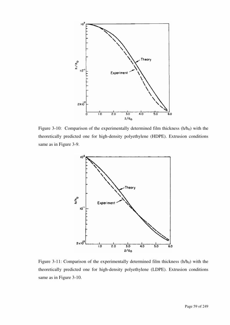
Page 59 of 249
Figure 3-10: Comparison of the experimentally determined film thickness (h/h0) with the
theoretically predicted one for high-density polyethylene (HDPE). Extrusion conditions
same as in Figure 3-9.
Figure 3-11: Comparison of the experimentally determined film thickness (h/h0) with the
theoretically predicted one for high-density polyethylene (LDPE). Extrusion conditions
same as in Figure 3-10.
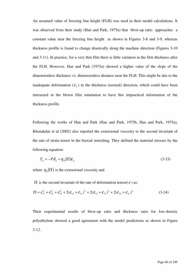
Page 60 of 249
An assumed value of freezing line height (FLH) was used in their model calculations. It
was observed from their study (Han and Park, 1975a) that blow-up ratio approaches a
constant value near the freezing line height as shown in Figures 3-8 and 3-9, whereas
thickness profile is found to change drastically along the machine direction (Figures 3-10
and 3-11). In practice, for a very thin film there is little variation in the film thickness after
the FLH. However, Han and Park (1975a) showed a higher value of the slope of the
dimensionless thickness vs. dimensionless distance near the FLH. This might be due to the
inadequate deformation ( 2εɺ ) in the thickness (normal) direction, which could have been
interacted in the blown film simulation to have this impractical information of the
thickness profile.
Following the works of Han and Park (Han and Park, 1975b, Han and Park, 1975a),
Khonakdar et al (2002) also reported the extensional viscosity to the second invariant of
the rate of strain tensor in the biaxial stretching. They defined the material stresses by the
following equation:
( )ijBijij
PT εηδ ɺΠ+−= (3-33)
where ( )ΠB
η is the extensional viscosity and
Π is the second invariant of the rate of deformation tensor(.
ε ) as:
2
3123
2
3113
2
2112
2
33
2
22
2
11 )(2)(2)(2 εεεεεεεεε ɺɺɺɺɺɺɺɺɺ ++++++++=Π (3-34)
Their experimental results of blow-up ratio and thickness ratio for low-density
polyethylene showed a good agreement with the model predictions as shown in Figure
3-12.
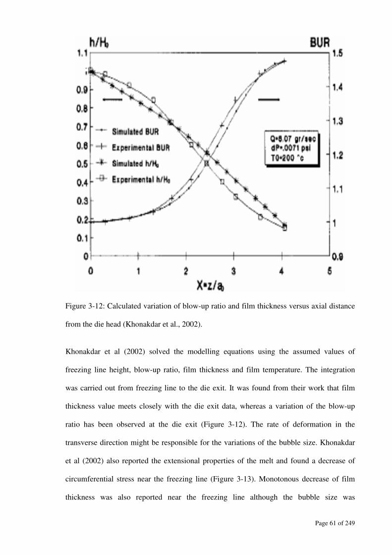
Page 61 of 249
Figure 3-12: Calculated variation of blow-up ratio and film thickness versus axial distance
from the die head (Khonakdar et al., 2002).
Khonakdar et al (2002) solved the modelling equations using the assumed values of
freezing line height, blow-up ratio, film thickness and film temperature. The integration
was carried out from freezing line to the die exit. It was found from their work that film
thickness value meets closely with the die exit data, whereas a variation of the blow-up
ratio has been observed at the die exit (Figure 3-12). The rate of deformation in the
transverse direction might be responsible for the variations of the bubble size. Khonakdar
et al (2002) also reported the extensional properties of the melt and found a decrease of
circumferential stress near the freezing line (Figure 3-13). Monotonous decrease of film
thickness was also reported near the freezing line although the bubble size was

Page 62 of 249
approaching to a constant value as shown in Figure 3-12. Hence, it is obvious that
deformation data did not incorporate well in their model (Khonakdar et al., 2002).
Figure 3-13: The total stress component versus axial distance from die exit (Khonakdar et
al., 2002).
3.4.3 Elastic Model
Pearson and Gutteridge (1978) developed an elastic model for the cold film blowing and
drawing process leading to bi-axial extension and orientation of crystalline polymer films.
They defined the stress tensor as:
R
R
T
R
F
WFFT
∂
∂−= .. (3-35)
where R
F ( xx ∂∂ /0 ) is the inverse of the deformation gradient tensor relating the
deformed(x) to the undeformed( 0x ) state and W is a strain energy function. Viscous effect
was not considered and there was no experimental verification of their work (Pearson and
Page 63 of 249
Gutteridge, 1978) (Figure 3-14). This was just an understanding and prediction of a
complicated mechanical process.
Figure 3-14: Dimensionless radius, temperature and velocity profiles for elastic model (a
is the dimensionless bubble radius,ϕ is the dimensional temperature based on elastic
modulus and u is the dimensionless film speed).
3.4.4 Maxwell Model
Luo and Tanner (1985) discussed the Maxwell model for both isothermal and non-
isothermal study of the blown film process. The constitutive equation was expressed as:
ijijijp δστ 0+= (3-36)
where ij
p δ0 is the pressure distribution, and
∂
∂+
∂
∂=+
∆
∆
i
j
j
i
ij
ij
x
v
x
v
t0ητ
τλ (3-37)

Page 64 of 249
where λ is the time constant, i
v are the velocity components along the i
x directions, and
the operator t∆
∆ is defined by:
kjikkijk
k
ij
k
ijij
LLx
vtt
τττττ
−−∂
∂+
∂
∂=
∆
∆ (3-38)
where the velocity gradient tensor ik
L is defined by
k
i
ik
x
vL
∂
∂= (3-39)
Similar to the Newtonian case, several typical bubble shapes were obtained for the
isothermal Maxwell model studied by Luo and Tanner (1985). The Maxwell model is
mathematically complex and instability of the numerical system was reported to integrate
from freezing line height to the die exit. Also, there was no experimental verification of the
predictions.
For the non-isothermal study of the Maxwell model, Luo and Tanner (1985) considered the
work of Gupta and Metzner (1982) and Gupta et al (1982) and discussed the bubble shapes
of fourteen non-isothermal runs (4 runs with BUR>1 and 10 runs with BUR<1). For the
four runs with BUR>1, a reasonable agreement of the experimental data was obtained.
However, no convergent results were obtained for BUR<1 due to the numerical instability.
Cain and Denn (1988) also reported the Maxwell model to determine the blown film
instabilities and avoided the multiple solutions with BUR>1 obtained from Newtonian
model. In their analysis, elastic effect near the freeze line height and multiple relaxation
time spectrums were not considered (Muke et al., 2003).
3.4.5 Viscoplastic-Elastic Modelling
Cao and Campbell (1990) developed a model for the liquid-solid transition from the die
exit to the nip rolls. They introduced the yield stress in the viscoelastic model and
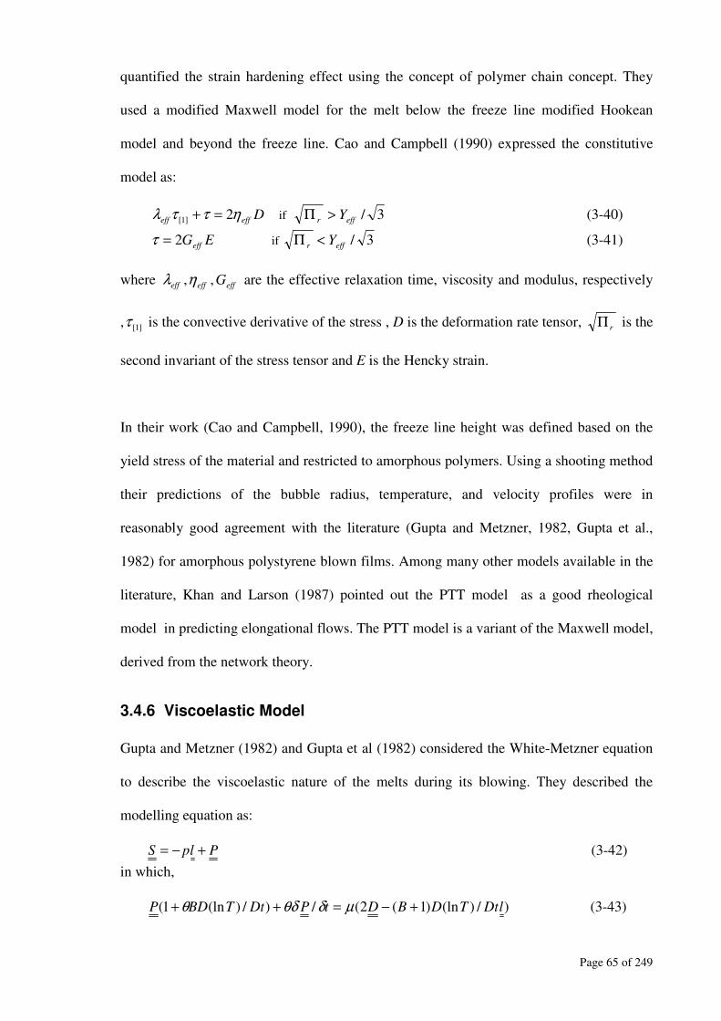
Page 65 of 249
quantified the strain hardening effect using the concept of polymer chain concept. They
used a modified Maxwell model for the melt below the freeze line modified Hookean
model and beyond the freeze line. Cao and Campbell (1990) expressed the constitutive
model as:
Deffeff
ηττλ 2]1[ =+ if 3/effr
Y>Π (3-40)
EGeff
2=τ if 3/effr
Y<Π (3-41)
where eff
λ ,eff
η ,eff
G are the effective relaxation time, viscosity and modulus, respectively
, ]1[τ is the convective derivative of the stress , D is the deformation rate tensor, r
Π is the
second invariant of the stress tensor and E is the Hencky strain.
In their work (Cao and Campbell, 1990), the freeze line height was defined based on the
yield stress of the material and restricted to amorphous polymers. Using a shooting method
their predictions of the bubble radius, temperature, and velocity profiles were in
reasonably good agreement with the literature (Gupta and Metzner, 1982, Gupta et al.,
1982) for amorphous polystyrene blown films. Among many other models available in the
literature, Khan and Larson (1987) pointed out the PTT model as a good rheological
model in predicting elongational flows. The PTT model is a variant of the Maxwell model,
derived from the network theory.
3.4.6 Viscoelastic Model
Gupta and Metzner (1982) and Gupta et al (1982) considered the White-Metzner equation
to describe the viscoelastic nature of the melts during its blowing. They described the
modelling equation as:
PlpS +−= (3-42)
in which,
)/)(ln)1(2(/)/)(ln1( lDtTDBDtPDtTBDP +−=++ µδθδθ (3-43)
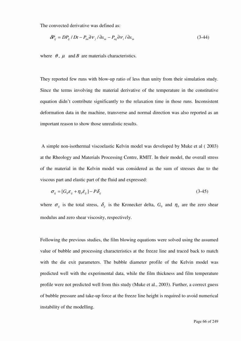
Page 66 of 249
The convected derivative was defined as:
mimjmjimijijxPxPDtDPP ∂∂−∂∂−= /// ννδ (3-44)
where θ , µ and B are materials characteristics.
They reported few runs with blow-up ratio of less than unity from their simulation study.
Since the terms involving the material derivative of the temperature in the constitutive
equation didn’t contribute significantly to the relaxation time in those runs. Inconsistent
deformation data in the machine, transverse and normal direction was also reported as an
important reason to show those unrealistic results.
A simple non-isothermal viscoelastic Kelvin model was developed by Muke et al ( 2003)
at the Rheology and Materials Processing Centre, RMIT. In their model, the overall stress
of the material in the Kelvin model was considered as the sum of stresses due to the
viscous part and elastic part of the fluid and expressed:
ijijijijPG δεηεσ −+= ][ 00
ɺ (3-45)
where ij
σ is the total stress, ij
δ is the Kronecker delta, 0G and 0η are the zero shear
modulus and zero shear viscosity, respectively.
Following the previous studies, the film blowing equations were solved using the assumed
value of bubble and processing characteristics at the freeze line and traced back to match
with the die exit parameters. The bubble diameter profile of the Kelvin model was
predicted well with the experimental data, while the film thickness and film temperature
profile were not predicted well from this study (Muke et al., 2003). Further, a correct guess
of bubble pressure and take-up force at the freeze line height is required to avoid numerical
instability of the modelling.
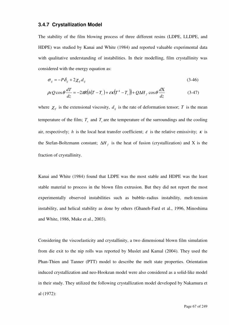
Page 67 of 249
3.4.7 Crystallization Model
The stability of the film blowing process of three different resins (LDPE, LLDPE, and
HDPE) was studied by Kanai and White (1984) and reported valuable experimental data
with qualitative understanding of instabilities. In their modelling, film crystallinity was
considered with the energy equation as:
ijtfijijdP χδσ 2+−= (3-46)
( ) ( )( )dz
dHQTTTThR
dz
dTcQ
fsc
Χ∆+−+−−= θεκπθρ cos2cos 4
(3-47)
where tf
χ is the extensional viscosity, ij
d is the rate of deformation tensor; T is the mean
temperature of the film; s
T and c
T are the temperature of the surroundings and the cooling
air, respectively; h is the local heat transfer coefficient; ε is the relative emissivity; κ is
the Stefan-Boltzmann constant; f
H∆ is the heat of fusion (crystallization) and X is the
fraction of crystallinity.
Kanai and White (1984) found that LDPE was the most stable and HDPE was the least
stable material to process in the blown film extrusion. But they did not report the most
experimentally observed instabilities such as bubble–radius instability, melt-tension
instability, and helical stability as done by others (Ghaneh-Fard et al., 1996, Minoshima
and White, 1986, Muke et al., 2003).
Considering the viscoelasticity and crystallinity, a two dimensional blown film simulation
from die exit to the nip rolls was reported by Muslet and Kamal (2004). They used the
Phan-Thien and Tanner (PTT) model to describe the melt state properties. Orientation
induced crystallization and neo-Hookean model were also considered as a solid-like model
in their study. They utilized the following crystallization model developed by Nakamura et
al (1972):
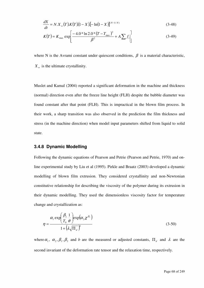
Page 68 of 249
( ) ( )( ) ( )[ ] )/1(1ln.1...
NN
XXTKTXNdt
dX −
∞ −−−= (3-48)
( )( )
+
−−= ∑ i
fATT
KTK .*0.2ln*0.4
exp2
2
max
maxβ
(3-49)
where N is the Avrami constant under quiescent conditions, β is a material characteristic,
∞X is the ultimate crystallinity.
Muslet and Kamal (2004) reported a significant deformation in the machine and thickness
(normal) direction even after the freeze line height (FLH) despite the bubble diameter was
found constant after that point (FLH). This is impractical in the blown film process. In
their work, a sharp transition was also observed in the prediction the film thickness and
stress (in the machine direction) when model input parameters shifted from liquid to solid
state.
3.4.8 Dynamic Modelling
Following the dynamic equations of Pearson and Petrie (Pearson and Petrie, 1970) and on-
line experimental study by Liu et al (1995). Pirkle and Braatz (2003) developed a dynamic
modelling of blown film extrusion. They considered crystallinity and non-Newtonian
constitutive relationship for describing the viscosity of the polymer during its extrusion in
their dynamic modelling. They used the dimensionless viscosity factor for temperature
change and crystallization as:
( )
( )b
d
T
Π+
=λ
χαθ
βα
η
β
1
exp1
exp 2
2
0
11
(3-50)
where 1α , 2α , 1β , 2β and b are the measured or adjusted constants, d
Π and λ are the
second invariant of the deformation rate tensor and the relaxation time, respectively.
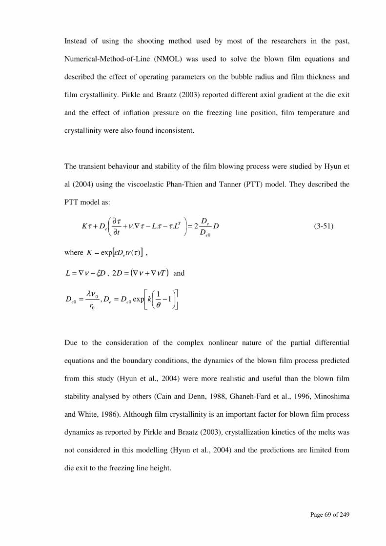
Page 69 of 249
Instead of using the shooting method used by most of the researchers in the past,
Numerical-Method-of-Line (NMOL) was used to solve the blown film equations and
described the effect of operating parameters on the bubble radius and film thickness and
film crystallinity. Pirkle and Braatz (2003) reported different axial gradient at the die exit
and the effect of inflation pressure on the freezing line position, film temperature and
crystallinity were also found inconsistent.
The transient behaviour and stability of the film blowing process were studied by Hyun et
al (2004) using the viscoelastic Phan-Thien and Tanner (PTT) model. They described the
PTT model as:
DD
DLL
tDK
e
eT
e
0
2... =
−−∇+
∂
∂+ τττν
ττ (3-51)
where [ ])(exp τε trDKe
= ,
DL ξν −∇= , ( )TD νν ∇+∇=2 and
−== 1
1exp, 0
0
0
0θ
λνkDD
rD
eee
Due to the consideration of the complex nonlinear nature of the partial differential
equations and the boundary conditions, the dynamics of the blown film process predicted
from this study (Hyun et al., 2004) were more realistic and useful than the blown film
stability analysed by others (Cain and Denn, 1988, Ghaneh-Fard et al., 1996, Minoshima
and White, 1986). Although film crystallinity is an important factor for blown film process
dynamics as reported by Pirkle and Braatz (2003), crystallization kinetics of the melts was
not considered in this modelling (Hyun et al., 2004) and the predictions are limited from
die exit to the freezing line height.

Page 70 of 249
3.5 Summary
Based on the previous studies on blown film modelling available in the literature, it can be
summarised that most rheological models used for simulation provided either inadequate
information of stress and material deformation during the film blowing or numerical
instability to solve them. Therefore, it is worthwhile to establish a new constitutive
equation to model the blown film processing. Model simulation should preferably be
attempted using a simple numerical technique to make accurate predictions of material
properties such as stress and rate of deformation. A further discussion of the development
of a new rheological constitutive equation and simulation results is presented in Chapter 7.
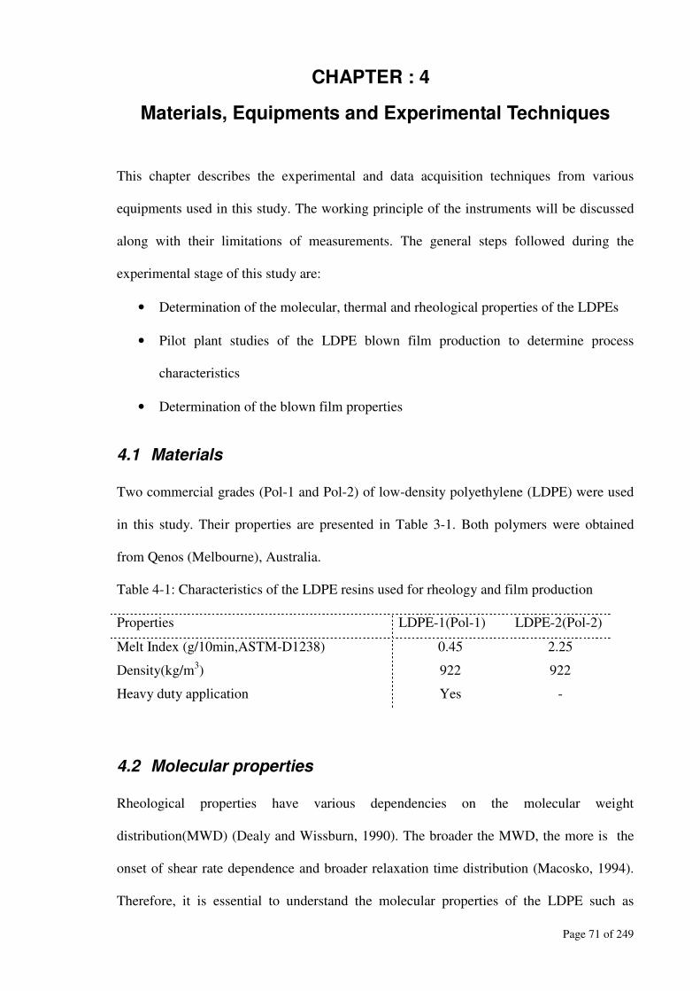
Page 71 of 249
CHAPTER : 4
Materials, Equipments and Experimental Techniques
This chapter describes the experimental and data acquisition techniques from various
equipments used in this study. The working principle of the instruments will be discussed
along with their limitations of measurements. The general steps followed during the
experimental stage of this study are:
• Determination of the molecular, thermal and rheological properties of the LDPEs
• Pilot plant studies of the LDPE blown film production to determine process
characteristics
• Determination of the blown film properties
4.1 Materials
Two commercial grades (Pol-1 and Pol-2) of low-density polyethylene (LDPE) were used
in this study. Their properties are presented in Table 3-1. Both polymers were obtained
from Qenos (Melbourne), Australia.
Table 4-1: Characteristics of the LDPE resins used for rheology and film production
Properties LDPE-1(Pol-1) LDPE-2(Pol-2)
Melt Index (g/10min,ASTM-D1238) 0.45 2.25
Density(kg/m3) 922 922
Heavy duty application Yes -
4.2 Molecular properties
Rheological properties have various dependencies on the molecular weight
distribution(MWD) (Dealy and Wissburn, 1990). The broader the MWD, the more is the
onset of shear rate dependence and broader relaxation time distribution (Macosko, 1994).
Therefore, it is essential to understand the molecular properties of the LDPE such as

Page 72 of 249
molecular weight and its distribution, degree of branching etc. due to their importance on
melt rheology, blown film processing and properties.
Gel permeation or size exclusion chromatography are the most common techniques to
determine the molecular properties (e.g., Mn, Mw, MWD, degree of branching etc.) of the
polymer (Cooper, 1989, Balke, 1984). The method of choice for determining the complete
MWD is the gel permeation chromatography (GPC) (Macosko, 1994).
4.2.1 Gel permeation chromatography (GPC)
During GPC experimentation, a solution containing the polymer of interest is pumped
down a column packed with a porous material. Due to diffusion, the polymers attempt to
enter the pores in the packing material. But only sufficiently small polymers can enter the
pores, and once they do, they are effectively trapped there until they exit again and return
to the flowing solvent. In this way, the small polymers are retarded and leave the GPC
column last. Various detectors are used to sense when the polymers finally emerge (or
“elute”) from the column. The time taken by the polymers to elute is converted to
molecular weight.
In order to determine the molecular properties, it is necessary to construct a master
calibration curve usually with narrow MWD polymers whose molecular weights are
known by some absolute method (e.g., light scattering, osmometry, mass spectroscopy or
analytical ultracentrifugation) and which would be valid for any level of branching
(Mendelson et al., 1970). The best polymer with which to calibrate the proposed system is
one having a similar persistence length (characteristic ratio) to the material considered for
GPC study.

Page 73 of 249
In this study, GPC analysis was performed at 140°C using a Waters Alliance GPCV2000
chromatographer (Figure 4-1), equipped with differential refractive index (DRI) and
viscometer detectors. 1, 2, 4-trichlorobenzene (TCB) was used as a solvent, with the flow
rate of 1.00 mL/min; the system of three Styragel® HT (4,5 and 6) columns were
calibrated with 10 narrow PS standards, with MPeak in the range of 1,000 to 5,000,000.
Chromatograms were processed using the Millennium® software. GPC information of
Pol-1 and Pol-2 are presented in Chapter 6 (Table 6-1).
Figure 4-1: Gel Permeation Chromatography (GPC) unit at the Rheology and Material
Processing Centre (RMPC) laboratory.
4.3 Rheological measurements
Rheological measurements have been differentiated into two categories:
• Shear (dynamic and steady) rheological measurements
• Extensional rheological measurement
Both data types will provide an understanding of the microstructure and morphology as
well as their response towards melt processing and properties of end products.
Page 74 of 249
4.3.1 Shear rheology
Both rotational rheometer (Advanced Rheometric Expansion System (ARES)) and
Capillary rheometer have been used in this study to determine the shear rheology of the
LDPEs. Steady shear rheological data from ARES rheometer were combined with
Capillary data to obtain the melt flow curve and zero shear viscosity of the polymers.
During shearing process, polymer samples can be degraded due to the long time residency
inside the hot chamber of the rheometer. At a particular shearing rate, this degradation time
is inversely related to the temperature. The effect of thermal degradation is significant on
the microstructure of the polymer, which can lead to chain scission, cross linking and other
physico-chemical processes (Dealy and Wissburn, 1990). Hence, more attention was paid
to avoid any unwanted phenomenon that can be carried out due to thermal degradation
during shear rheological measurements.
4.3.1.1 Measurement of dynamic shear rheology
Dynamic tests include the determination of linear viscoelastic regions (using dynamic
strain sweep test) to separate the corresponding viscous and elastic properties (using
dynamic frequency sweeps) of the LDPEs. Determination of the linear viscoelastic region
is essential before commencing dynamic frequency sweep test to ensure that the
microstructure of the material would not be affected by shear alignment. The conditions
that satisfy linear viscoelasticity are that the stress is linearly proportional to the imposed
strain and the torque response involves only the first harmonic (Ferry J.D., 1980). In the
linear viscoelastic region, both the storage ( )G′ and loss ( )G ′′ moduli are expected to be
independent of the strain amplitude and there will be a proportional increment of stress.
This constant of proportionality is the modulus. The absence of higher harmonics for the
stress response ensures that it remains sinusoidal, thus obeying the second condition.

Page 75 of 249
Parallel plate and torsional flow rheometers are the most common equipment used to
determine the viscoelasticity of the polymer melt (Macosko, 1994). In this study, parallel
plate rheometer is used to determine shear rheology of the LDPE melts.
4.3.1.1.1 Parallel plate rheometer
Determination of shear rheology (dynamic and steady) using parallel plate geometry
(Figure 4-2) was first suggested by Mooney and Ewart (1934). Generally, in a parallel
plate, samples are loaded between the plates that are separated by a height, h. The lower
plate oscillates (dynamic measurements) or rotates (steady shear measurements) at a
constant angular velocity (Ω). The upper plate measures torque (M) and normal stress
functions (N1 and N2) (Powell R., 1998). These parameters are related to the shear stress
(Equation 4-1) and normal stress function (Equation 4-2). Powell R (1998), Macosko
(1994) and Morrison (2001) described in detail in the derivation of the shear viscosity and
normal stress functions.
Figure 4-2: Schematic of a parallel plate rheometer (Macosko, 1994)
+=
Rd
Md
R
M
γπτ
ɺln
ln3
2 312 (4-1)
( ) ( )
+=−
R
ZZ
RR
d
Fd
R
FNN
γπγγ
ɺ
ɺɺ
ln
ln
2
11
2221 (4-2)

Page 76 of 249
where 12τ is the shear stress that is based on the rim of the plates, R is the radius of the
plate (centre to rim); R
γɺ is the shear rate based on the rim of the plates; z
F is the normal
force.
Although parallel plate geometry is relatively user friendly, a drawback is that shear rate
varies radially along the plates, hence shear rate is not constant throughout the sample
(Mackay, 1993). This apparent shear rate (due to its dependency on radial position) is
calculated using Equation 4-3.
h
R
R
Ω=γɺ (4-3)
Parallel plate geometries, however, are useful with small amplitude oscillatory shear
(SAOS) (Morrison, 2001). The SAOS material functions ( )η ′ and ( )η ′′ can be related to
measured torque, and phase lag ( )δ by using Equations 4-4 and 4-5 (Morrison, 2001). The
former is the dynamic viscosity, while the latter is the out-of-phase component of complex
viscosity (η ∗). θο, in Equations 4-4 and 4-5 refers to angular amplitude for oscillatory shear
(Dealy and Wissburn, 1990).
( )θωπ
δωη
0
4
sin2
R
hM=′ (4-4)
( )θωπ
δωη
0
4
cos2
R
hM=′′ (4-5)
In the parallel plate rheometer, a particular sample type (usually moulded plaque) and
sample dimensions (thickness and diameter) are required. In this study, a 2mm thick
plaque was cut into 25mm and 50mm diameter disks to use in the Advanced Rheometric
Expansion System (ARES) rotational rheometer.
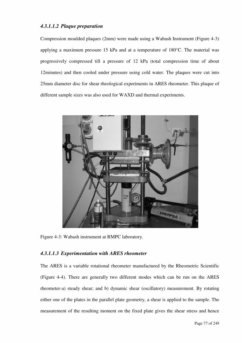
Page 77 of 249
4.3.1.1.2 Plaque preparation
Compression moulded plaques (2mm) were made using a Wabash Instrument (Figure 4-3)
applying a maximum pressure 15 kPa and at a temperature of 180°C. The material was
progressively compressed till a pressure of 12 kPa (total compression time of about
12minutes) and then cooled under pressure using cold water. The plaques were cut into
25mm diameter disc for shear rheological experiments in ARES rheometer. This plaque of
different sample sizes was also used for WAXD and thermal experiments.
Figure 4-3: Wabash instrument at RMPC laboratory.
4.3.1.1.3 Experimentation with ARES rheometer
The ARES is a variable rotational rheometer manufactured by the Rheometric Scientific
(Figure 4-4). There are generally two different modes which can be run on the ARES
rheometer-a) steady shear; and b) dynamic shear (oscillatory) measurement. By rotating
either one of the plates in the parallel plate geometry, a shear is applied to the sample. The
measurement of the resulting moment on the fixed plate gives the shear stress and hence
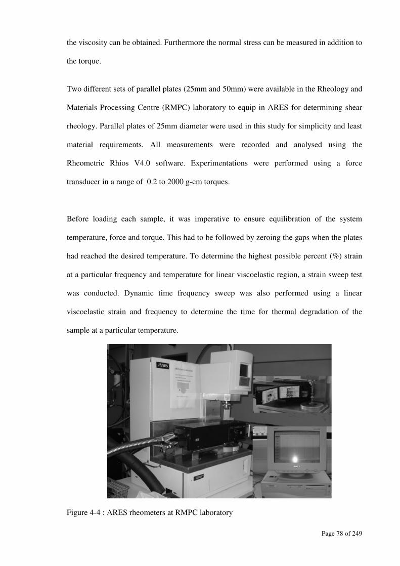
Page 78 of 249
the viscosity can be obtained. Furthermore the normal stress can be measured in addition to
the torque.
Two different sets of parallel plates (25mm and 50mm) were available in the Rheology and
Materials Processing Centre (RMPC) laboratory to equip in ARES for determining shear
rheology. Parallel plates of 25mm diameter were used in this study for simplicity and least
material requirements. All measurements were recorded and analysed using the
Rheometric Rhios V4.0 software. Experimentations were performed using a force
transducer in a range of 0.2 to 2000 g-cm torques.
Before loading each sample, it was imperative to ensure equilibration of the system
temperature, force and torque. This had to be followed by zeroing the gaps when the plates
had reached the desired temperature. To determine the highest possible percent (%) strain
at a particular frequency and temperature for linear viscoelastic region, a strain sweep test
was conducted. Dynamic time frequency sweep was also performed using a linear
viscoelastic strain and frequency to determine the time for thermal degradation of the
sample at a particular temperature.
Figure 4-4 : ARES rheometers at RMPC laboratory
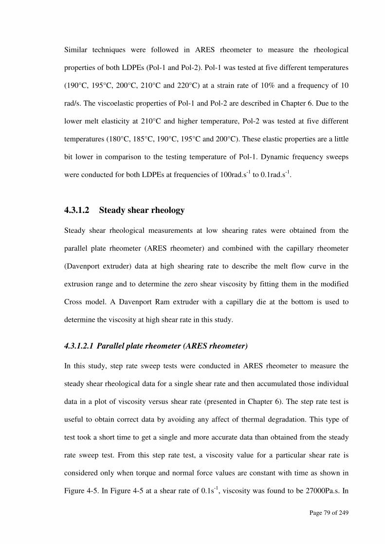
Page 79 of 249
Similar techniques were followed in ARES rheometer to measure the rheological
properties of both LDPEs (Pol-1 and Pol-2). Pol-1 was tested at five different temperatures
(190°C, 195°C, 200°C, 210°C and 220°C) at a strain rate of 10% and a frequency of 10
rad/s. The viscoelastic properties of Pol-1 and Pol-2 are described in Chapter 6. Due to the
lower melt elasticity at 210°C and higher temperature, Pol-2 was tested at five different
temperatures (180°C, 185°C, 190°C, 195°C and 200°C). These elastic properties are a little
bit lower in comparison to the testing temperature of Pol-1. Dynamic frequency sweeps
were conducted for both LDPEs at frequencies of 100rad.s-1
to 0.1rad.s-1
.
4.3.1.2 Steady shear rheology
Steady shear rheological measurements at low shearing rates were obtained from the
parallel plate rheometer (ARES rheometer) and combined with the capillary rheometer
(Davenport extruder) data at high shearing rate to describe the melt flow curve in the
extrusion range and to determine the zero shear viscosity by fitting them in the modified
Cross model. A Davenport Ram extruder with a capillary die at the bottom is used to
determine the viscosity at high shear rate in this study.
4.3.1.2.1 Parallel plate rheometer (ARES rheometer)
In this study, step rate sweep tests were conducted in ARES rheometer to measure the
steady shear rheological data for a single shear rate and then accumulated those individual
data in a plot of viscosity versus shear rate (presented in Chapter 6). The step rate test is
useful to obtain correct data by avoiding any affect of thermal degradation. This type of
test took a short time to get a single and more accurate data than obtained from the steady
rate sweep test. From this step rate test, a viscosity value for a particular shear rate is
considered only when torque and normal force values are constant with time as shown in
Figure 4-5. In Figure 4-5 at a shear rate of 0.1s-1
, viscosity was found to be 27000Pa.s. In
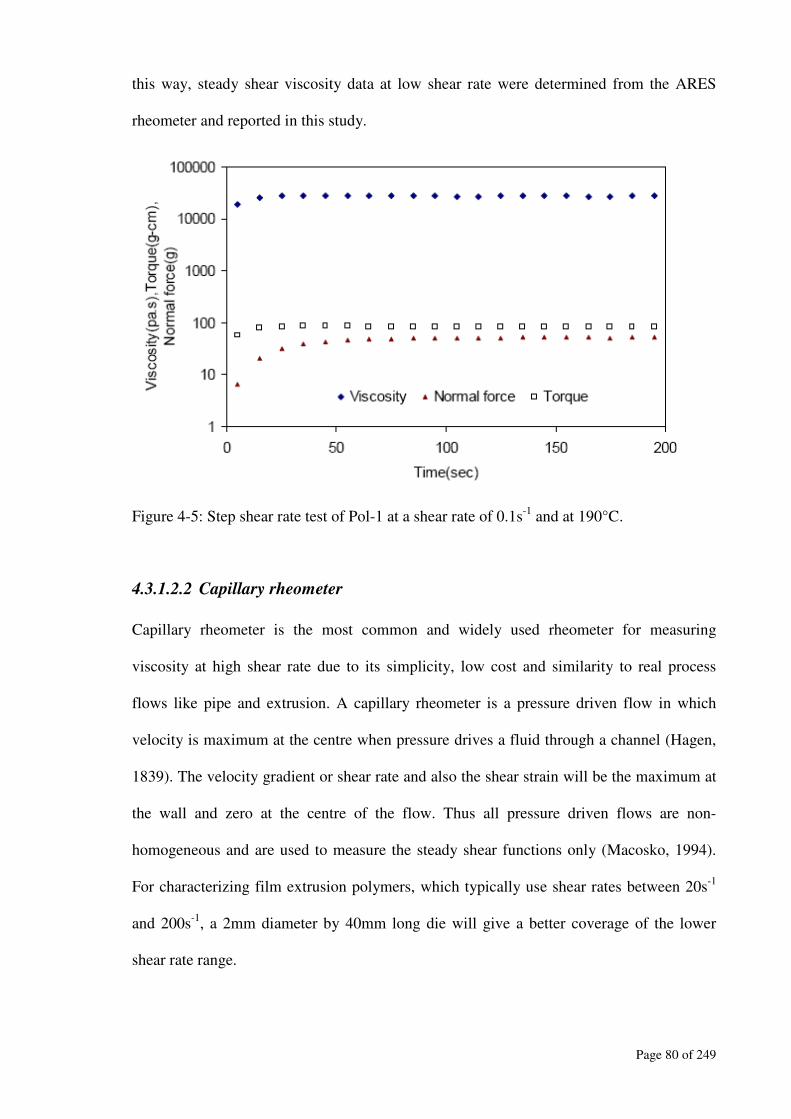
Page 80 of 249
this way, steady shear viscosity data at low shear rate were determined from the ARES
rheometer and reported in this study.
Figure 4-5: Step shear rate test of Pol-1 at a shear rate of 0.1s-1
and at 190°C.
4.3.1.2.2 Capillary rheometer
Capillary rheometer is the most common and widely used rheometer for measuring
viscosity at high shear rate due to its simplicity, low cost and similarity to real process
flows like pipe and extrusion. A capillary rheometer is a pressure driven flow in which
velocity is maximum at the centre when pressure drives a fluid through a channel (Hagen,
1839). The velocity gradient or shear rate and also the shear strain will be the maximum at
the wall and zero at the centre of the flow. Thus all pressure driven flows are non-
homogeneous and are used to measure the steady shear functions only (Macosko, 1994).
For characterizing film extrusion polymers, which typically use shear rates between 20s-1
and 200s-1
, a 2mm diameter by 40mm long die will give a better coverage of the lower
shear rate range.
Page 81 of 249
Steady shear rheological measurements at low shearing rates were obtained from ARES
rheometer and combined with the capillary data at high shearing rate to describe the melt
flow curve in the extrusion range and to determine the zero shear viscosity by fitting them
in the modified Cross model. Steady shear rheological properties were determined using
step rate test (rheological properties for a single shear rate) in the transient mode of ARES
ranging from 0.01s-1
to 1.0 s-1
. Davenport Ram extruder with a capillary die was used to
determine the viscosity at high shear rate in this study.
4.3.1.2.3 Davenport Ram extruder
The Ram extruder (Figure 4-6) contains a capillary die, held in place at the base of the pot
by means of a screw-in die-retainer. A close fitting piston is driven at constant speed and
the resulting pressure recorded by a melt-pressure transducer mounted in the wall of the
pot, close to the die entry. The choice of die diameter is governed by the shear range
required and operating pressure will increase or decrease with the die diameter. The choice
of transducer depends on the MFI of the polymer and the temperature used.
Figure 4-6 : Davenport Ram Extruder at RMPC laboratory.
Page 82 of 249
The barrel of the Ram extruder was filled with the polymer pellets which were allowed to
melt them properly at an experimental temperature before the piston was driven
downwards for melt flow. A transducer of 10,000psi and two different dies (diameter of
2mm and 4mm and land length of 31mm) were used in this study. Similar temperatures
were chosen for both polymers as were used in ARES for steady shear measurements. Wall
shear rate was corrected using the power law index (n) and the Rabinowitsch method to
evaluate the experimental data.
4.3.2 Extensional rheology
Extensional rheological measurements play an important role in simulating many industrial
processes like film blowing, fibre spinning and blow moulding. This flow field involves
orientation of molecular structures in the flow direction and at high deformation rates,
typical of industrial processes (Gupta R.K., 1998). The industrial extensional deformation
has short durations and produces large fluid stresses. There are three principal extensional
deformations, uniaxial, biaxial and planar. In this study, uniaxial extensional deformations
of the LDPEs have been considered to determine their strain hardening behaviour and
extensional rheology. The equipment used in this study is the Meissner-type Rheometric
Melt Extensional (RME) rheometer.
4.3.2.1 Measurement of the extensional viscosity
Homogeneous (voids and stress free) samples are required for the extensional rheometers
otherwise the true strain rate varies within the samples. Sample preparation for the RME
was performed by compression moulding of the LDPE pellets using a smooth and finished
mild steel moulds. The procedure has been described earlier (Section 4.3.1.1.2) for sheet
compression moulding. The process was optimised by trial and error approach and assured
production of flat, homogeneous and relatively stress-free plaques, 1.5 - 2 mm thick. The
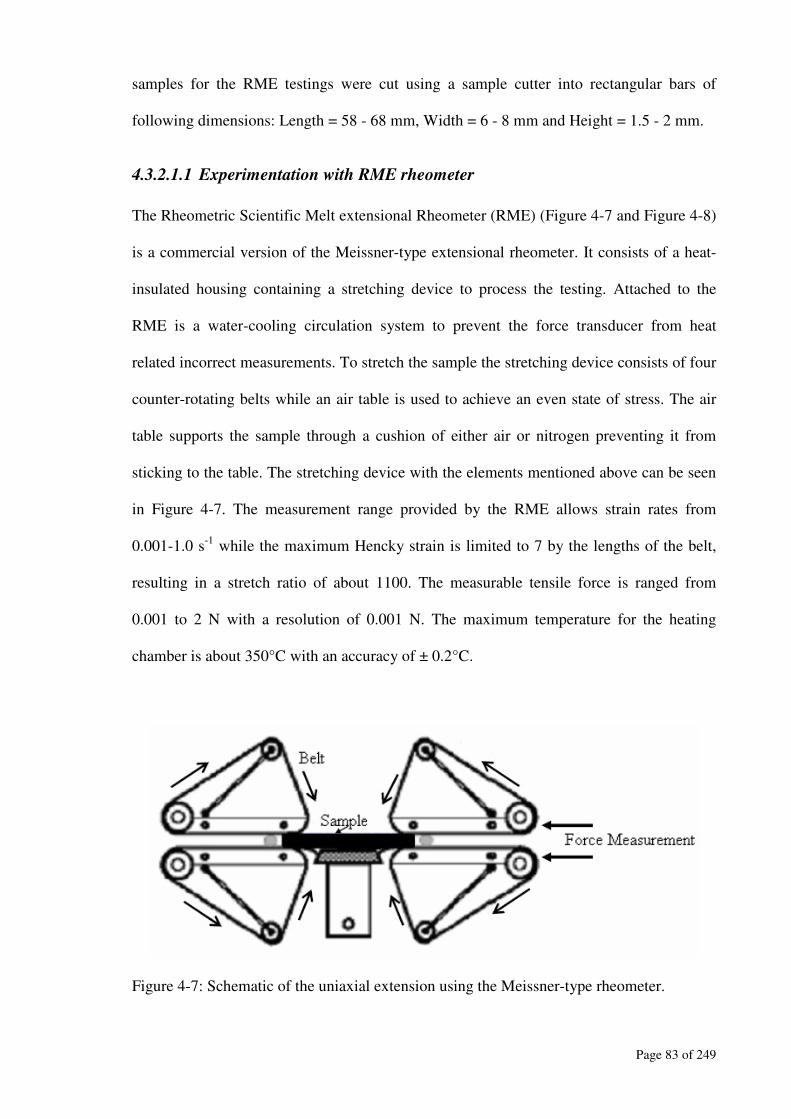
Page 83 of 249
samples for the RME testings were cut using a sample cutter into rectangular bars of
following dimensions: Length = 58 - 68 mm, Width = 6 - 8 mm and Height = 1.5 - 2 mm.
4.3.2.1.1 Experimentation with RME rheometer
The Rheometric Scientific Melt extensional Rheometer (RME) (Figure 4-7 and Figure 4-8)
is a commercial version of the Meissner-type extensional rheometer. It consists of a heat-
insulated housing containing a stretching device to process the testing. Attached to the
RME is a water-cooling circulation system to prevent the force transducer from heat
related incorrect measurements. To stretch the sample the stretching device consists of four
counter-rotating belts while an air table is used to achieve an even state of stress. The air
table supports the sample through a cushion of either air or nitrogen preventing it from
sticking to the table. The stretching device with the elements mentioned above can be seen
in Figure 4-7. The measurement range provided by the RME allows strain rates from
0.001-1.0 s-1
while the maximum Hencky strain is limited to 7 by the lengths of the belt,
resulting in a stretch ratio of about 1100. The measurable tensile force is ranged from
0.001 to 2 N with a resolution of 0.001 N. The maximum temperature for the heating
chamber is about 350°C with an accuracy of ± 0.2°C.
Figure 4-7: Schematic of the uniaxial extension using the Meissner-type rheometer.

Page 84 of 249
Figure 4-8 : RME rheometer at RMPC laboratory.
The strain is applied by a certain velocity of two pairs of counter-rotating conveyor belts
clamping the sample on both ends. These aluminium conveyor belts are equipped with
threads to avoid slippage of the sample while elongating. As the polymer sample is molten,
a cushion of nitrogen or air is generated between the air table and the sample to support the
sample. Furthermore metal tongues attached to the lower belts prevent the melt from
flowing into the gap between the air table and the belts. To heat up and melt the sample,
both the gas cushion and the heating chamber are used.
Both LDPEs (Pol-1 and Pol-2) were tested at three different temperatures (140°C, 150°C
and 170°C) and at three different strain rates (0.1s-1
, 0.5s-1
and 1.0s-1
). The sample was
placed into the RME rheometer properly to provide a uniform stretching. It means that the
belt tongues were perfectly placed to prevent the sample from sticking to the table or
flowing to the gap. All measurements were recorded and analysed using the Rheometric
software (version 1.7) provided with the RME rheometer.

Page 85 of 249
4.4 Experimentation with Wide angle X-ray Diffraction (WAXD)
WAXD was used to determine the crystalline peaks and width of the intensity of the
processed films in both machine and transverse directions. A Phillips X-Ray generator
(Philips PW 1130, Holland) (Figure 4-9) using a 30kV of accelerating voltage and 20mA
of current were used for experimentation. Intensities from diffraction angle (2θ) =10° to
40° were recorded using Ni filtered Cu-Kα radiation (λ=1.54Ǻ). Sample plaques of both
resins were made using identical methods (200°C and 120kN) for XRD experiments.
Figure 4-9: Phillips X-Ray generator at RMPC laboratory
4.5 Experimentation with Modulated Differential Scanning
Calorimetry (MDSC)
The MDSC instrument consists of a reference and sample holder which is individually
heated in the presence of a nitrogen atmosphere. The melting and crystallization temperature
of the polymers were determined by measuring the difference in the heat flow between the

Page 86 of 249
sample and reference. When the melting temperature of the polymer is attained, the polymer
absorbs thermal energy so that the increase in heat flow occurs in order to maintain the two
heating curves (heating curves for the sample and reference holder) at the same temperature.
When the crystallization temperature of the polymer is reached, it releases thermal energy
and therefore less heat is required to flow to the sample holder.
Figure 4-10: TA instrument (MDSC-2920) at RMPC laboratory
In this study, thermal treatments of the pellets, plaques and film samples were performed
using the Modulated Differential Scanning Calorimetry (MDSC-2920 with thermal analyst
3100 software, TA Instruments, USA) (Figure 4-10). Cell constant determination and
temperature calibration of this instrument was accomplished using a known sample (Indium,
melting point=156.28°C and standard heat=28.42 j/g). Using a sophisticated balance,
samples of 5-10mg were prepared by cutting the polymer pellets, plaques or films and
placed into the Aluminium pan with lid. Samples were heated from 20°C to 180°C and
cooled to 20°C. Tests were conducted using helium as purge gas (30 ml/min flow rate) and
nitrogen as environment gas (100 ml/min flow rate). The heating and cooling rate were
constant at 2°C/min using 0.5°C modulation amplitude and at a 40 sec modulation period.

Page 87 of 249
Crystalline properties of the film were determined using the heat of fusion of the sample
(Samplef
H ,∆ ) and standard heat (reference value represents the heat of melting if the polymer
were 100% crystalline,tyCrystalinif
H %100,∆ ) (Equation 4-6) from the first the heating cycle.
%100%%100,
,x
H
HityCrystallin
tyCrystalinif
Samplef
∆
∆= (4-6)
4.6 Blown film production
A general full factorial statistical design using MINITAB-14 was used for the design of
experiments (DOE). Die temperature and cooling rate (blower setting or speed) were used
as the factor with 3 and 4 levels respectively. An Advanced Blown Film Extrusion System
with co-extrusion assembly manufactured by Future Design Inc was used to process the
LDPEs.
Figure 4-11: Blown film production using the Advanced Blown Film Extrusion System at
AMCOR Research & Technology, Melbourne.
Page 88 of 249
In this study, a co-extrusion assembly equipped with an annular die was used for extrusion
of the LDPEs. The film blowing process (Figure 4-11) was initiated by pulling the molten
polymer leaving the die and passed over the nip rollers. Inflation of the polymer bubble
was accompanied by increasing the air flow inside the bubble. Additional cooling was also
provided inside and outside of the molten bubble. The action of the nip rollers provided the
axial tension and also formed an airtight seal so that a constant pressure could be
maintained in the bubble. The nip roller speed and the amount of air inside the bubble were
adjusted to achieve a desired value of blow up ratio (BUR) and draw down ratio (DDR)
according to the design of experiment.
The mass flow rate of the film was determined by weighing the amount of film produced at
two minutes intervals. Average data of the mass flow rate was considered from five set of
measurements. This information combined with the die geometry and melt density was
used to determine the die exit velocity using conservation law of mass. Nip roller speed
was determined from the digital data provided by the equipment. At a certain distance from
the die exit, the bubble diameter was found constant in the axial direction with respect to
the vertical axis. Usually, melt bubble is frozen or solidified or crystallized after covering
certain axial distance. An average value of the lower and upper limit of the freezing zone is
termed as the freeze line height. Lower limit of the freezing zone was easy to trace and
considered as the freeze line height (FLH) in the blown film simulation. It was observed
that with the increase of cooling rate, FLH goes down. Bubble diameter was calculated
using the lay flat width of the film (Equation 4-7). Film thickness was determined using a
digital micrometer. Temperature was determined using an infra red pyrometer (Model IR-
TA manufactured by Chino Corp). The advantage of using the infra red pyrometer is that it
is a non-contact and user friendly device to measure the temperature. The instrument
absorbs the infra red radiation in a wavelength of 3.43µm. The temperature reading with

Page 89 of 249
this wavelength represents the surface temperature of the bubble. Instrument calibration
was performed by adjusting the emissivity of the pyrometer. Take-up ratio (TUR) was
determined by dividing the nip roller speed with die exit velocity. An average value of lay
flat width (LFW) was considered from the ten data samples of the solid film bubble to
determine the blow up ratio (BUR) using the following equation (Equation 4-7):
d
LFWxBUR
π2= (4-7)
4.6.1 Extruder geometries and process parameters
An Advanced Blown Film co-extrusion assembly (diameter= 20mm, L/D=30:1 and
compression ratio=2.2:1 for Screw-1 and Screw-3 and diameter= 25mm, L/D=30:1 and
compression ratio=2.8:1 for Screw-2) manufactured by Future Design Inc was used to
process the LDPEs at AMCOR Research and Technology’s pilot plant. A sample data
sheet used for blown film production is presented in the Appendix (Table A1-1). A 2.032
mm die gap and 65 mm die diameter was used. Films were produced at three different die
temperatures (200°C, 210°C and 220°C) and four different blower settings 2.4, 2.6, 2.8 and
3.0 which correspond to an average air velocity of 6.7, 7.2, 7.7 and 8.2 m/s respectively
outside of the bubble. Air flow inside the bubble was kept constant.
The LDPEs were processed at identical processing conditions used in blown film
extrusion. Blow up ratio (BUR) and draw down ratio (DDR) were kept constant at 2.35
and 21.4 respectively. Standard deviation of BUR and DDR calculation was less than 0.5.
RPM of the screws was kept constant. Average mass flow rate of the extrusion was about
7.4 kg/hr for both polymers. Average nip roller speed was 180 m/hr and winder tension
was kept constant throughout the trial. Film thickness for both resins varied from 110-120
micrometer (µm) during processing.
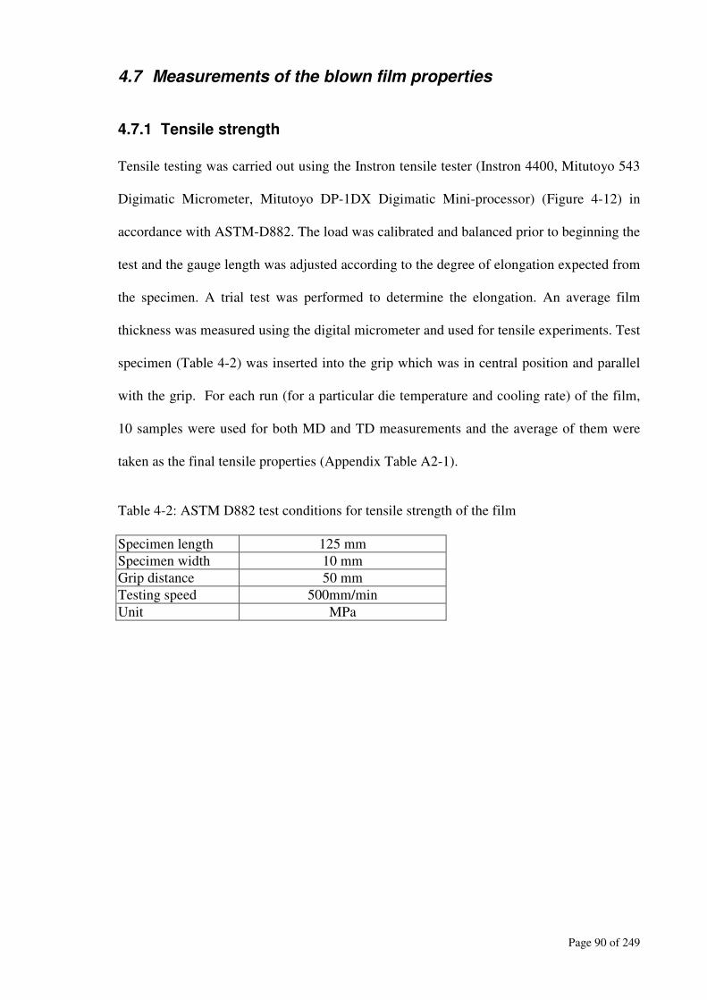
Page 90 of 249
4.7 Measurements of the blown film properties
4.7.1 Tensile strength
Tensile testing was carried out using the Instron tensile tester (Instron 4400, Mitutoyo 543
Digimatic Micrometer, Mitutoyo DP-1DX Digimatic Mini-processor) (Figure 4-12) in
accordance with ASTM-D882. The load was calibrated and balanced prior to beginning the
test and the gauge length was adjusted according to the degree of elongation expected from
the specimen. A trial test was performed to determine the elongation. An average film
thickness was measured using the digital micrometer and used for tensile experiments. Test
specimen (Table 4-2) was inserted into the grip which was in central position and parallel
with the grip. For each run (for a particular die temperature and cooling rate) of the film,
10 samples were used for both MD and TD measurements and the average of them were
taken as the final tensile properties (Appendix Table A2-1).
Table 4-2: ASTM D882 test conditions for tensile strength of the film
Specimen length 125 mm
Specimen width 10 mm
Grip distance 50 mm
Testing speed 500mm/min
Unit MPa
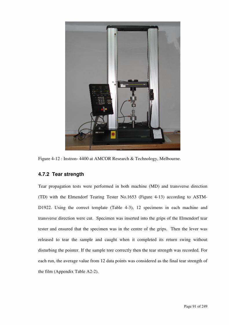
Page 91 of 249
Figure 4-12 : Instron- 4400 at AMCOR Research & Technology, Melbourne.
4.7.2 Tear strength
Tear propagation tests were performed in both machine (MD) and transverse direction
(TD) with the Elmendorf Tearing Tester No.1653 (Figure 4-13) according to ASTM-
D1922. Using the correct template (Table 4-3), 12 specimens in each machine and
transverse direction were cut. Specimen was inserted into the grips of the Elmendorf tear
tester and ensured that the specimen was in the centre of the grips. Then the lever was
released to tear the sample and caught when it completed its return swing without
disturbing the pointer. If the sample tore correctly then the tear strength was recorded. For
each run, the average value from 12 data points was considered as the final tear strength of
the film (Appendix Table A2-2).

Page 92 of 249
Table 4-3: ASTM D1922 test conditions for tear strength of the film
Specimen length 76 mm
Specimen width 63 mm
Unit mN
Figure 4-13: Elmendorf Tearing Tester (No.1653) at AMCOR Research & Technology,
Melbourne.
4.7.3 Dart impact strength
Dart impact test (Figure 4-14) determines the weight required to cause failure of the test
sample (Table 4-4) by carrying out several practice dart drops. The incremental weight to
be used in the test will be 5% to 15% of the failure weight. The loaded dart was dropped on
the sample at least 20 times, where at least 10 drops produce a failure and at least 10
produce a non-failure. Each time the sample fails, the weight on the dart is decreased by
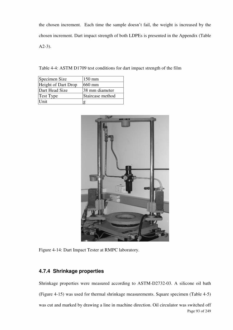
Page 93 of 249
the chosen increment. Each time the sample doesn’t fail, the weight is increased by the
chosen increment. Dart impact strength of both LDPEs is presented in the Appendix (Table
A2-3).
Table 4-4: ASTM D1709 test conditions for dart impact strength of the film
Specimen Size 150 mm
Height of Dart Drop 660 mm
Dart Head Size 38 mm diameter
Test Type Staircase method
Unit g
Figure 4-14: Dart Impact Tester at RMPC laboratory.
4.7.4 Shrinkage properties
Shrinkage properties were measured according to ASTM-D2732-03. A silicone oil bath
(Figure 4-15) was used for thermal shrinkage measurements. Square specimen (Table 4-5)
was cut and marked by drawing a line in machine direction. Oil circulator was switched off

Page 94 of 249
and specimen was submerged into the oil bath and kept for 20 seconds. After thermal
treatment, samples were cooled in a water bath. The length and width of shrank specimens
were measured. Difference between original length and shrunk length was used to
calculate the percentage shrinkage in corresponding direction of film. For each run, five
samples were submerged into the bath and their average values were taken as the final
shrinkage (Appendix Tables A2-4 and A2-5).
Table 4-5: ASTM D2732-03 test conditions for shrinkage of the film
Apparatus Silicone oil bath
Temperature 125°C
Specimen length 100 mm
Specimen width 100 mm
Shrinking time 20 seconds
Units %
Figure 4-15: Shrinkage testing silicone oil bath at AMCOR Research & Technology,
Melbourne.

Page 95 of 249
4.7.5 Optical properties (haze and gloss)
According to the ASTM-D1003, GARDNER haze meter, Model-UX10 and PG-5500
digital photometric unit were used for the haze measurement. Before taking any reading,
the instrument was calibrated according to the operating manual. The test sample (Table
4-6) was inserted into the specimen holder, and the photometric unit took the reading. Six
samples were measured for each run and their average value was used for analysis
(Appendix Table A2-6).
Table 4-6: ASTM D1003 test conditions for haze properties of the film
Specimen length 100 mm
Specimen width 100 mm
Unit %
Gloss measures the shininess of the film. A BYK Gardner gloss meter (micro gloss-45°)
was used for gloss measurement according to ASTM-D2457. An incandescent light source
is directed at the test specimen at a specified incidence angle (45° in this study) (Figure
4-16). A receptor is located at the mirror reflection of the incident beam. Polished black
glass with a refractive index of 1.567 was used as a standard. At least 10 data points were
taken in both MD and TD and their average value was considered as the final gloss of that
film (Appendix table A2-7).
Figure 4-16: Schematic of gloss meter.
Page 96 of 249
4.8 Summary
This chapter summarises various experimental techniques used in this research. A lot of
attention was paid for all experimentations to obtain error free data. Most of the
equipments used in this study are digitally controlled and new and sophisticated such as
ARES rheometer, MDSC-2920, GPC, blown film pilot plant, Instron-4400, Haze and
Gloss meter.
However, rheological properties are sensitive to temperature, thermal degradation of the
sample (due to longer residence time in the rheometer), melt flow instability, melt fracture
and other instrumental defects or limitations. It is also necessary to check the instrumental
sensitivity of the WAXD and MDSC experiments. Therefore, error analyses of these data
are presented in Chapter 5.
Pilot plant study of the blown film production was carried out using an identical design of
experiment for both LDPEs. Pilot plant data and blown film properties are presented in the
Appendix section (A1 and A2). Average value of the blown film properties were
considered for statistical analysis with respect to die temperature and cooling rate. These
statistical analyses are presented in Chapter 8.
Page 97 of 249
CHAPTER : 5
Error Analysis
This chapter aims to briefly discuss the sources of error arising from experimental
measurements and the techniques applied to correct or eliminate them. The accuracy of the
experimental data has been discussed here.
5.1 Dynamic shear measurements
Dynamic (oscillatory) shear rheology is a reflection of molecular characteristics of the
polymer. Dynamic shear measurements involved dynamic strain, time and frequency
sweeps. The important aspects of dynamic shear measurements that need to be considered
in this study are:
• Determination of linear viscoelastic region for molecular properties of the
polymers
• Thermal degradation of samples that usually happened at elevated temperatures and
during long time experimentation.
• Repeatability of the runs to ensure self consistency of measurements.
• Reliability of measurement at low frequencies which may be related in the limit of
instrument sensitivity.
Sensitivity of the storage modulus (represents the elastic nature of the polymer) is higher
than loss modulus on linear viscoelastic properties (Prasad, 2004). Therefore, linear
viscoelastic strain and time were determined based on storage modulus response.
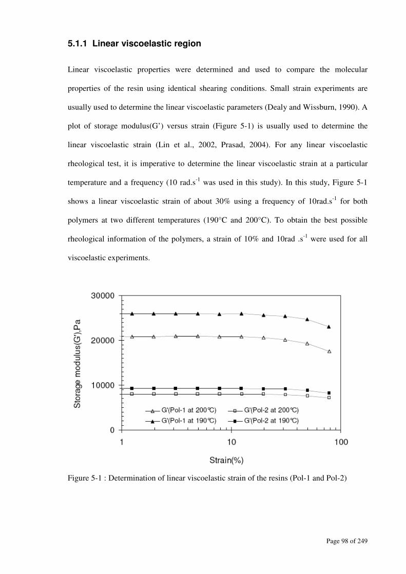
Page 98 of 249
5.1.1 Linear viscoelastic region
Linear viscoelastic properties were determined and used to compare the molecular
properties of the resin using identical shearing conditions. Small strain experiments are
usually used to determine the linear viscoelastic parameters (Dealy and Wissburn, 1990). A
plot of storage modulus(G’) versus strain (Figure 5-1) is usually used to determine the
linear viscoelastic strain (Lin et al., 2002, Prasad, 2004). For any linear viscoelastic
rheological test, it is imperative to determine the linear viscoelastic strain at a particular
temperature and a frequency (10 rad.s-1
was used in this study). In this study, Figure 5-1
shows a linear viscoelastic strain of about 30% using a frequency of 10rad.s-1
for both
polymers at two different temperatures (190°C and 200°C). To obtain the best possible
rheological information of the polymers, a strain of 10% and 10rad .s-1
were used for all
viscoelastic experiments.
Figure 5-1 : Determination of linear viscoelastic strain of the resins (Pol-1 and Pol-2)

Page 99 of 249
5.1.2 Thermal degradation
An extra attention was carried out during the experimental work of this study so that
rheological data becomes unaffected by thermal degradation. Experimental time of thermal
degradation was determined using a dynamic time sweep test (using strain=10% and
frequency=10 rad.s-1
) at all experimental temperatures used in this research. Figure 5-2
shows the time sweep test of the LDPEs (Pol-1 and Pol-2) at 200°C. Although, storage
modulus data is more sensitive to thermal degradation, both storage and loss modulus data
were checked in this study (Figure 5-2) to determine the time for linear viscoelastic
experiment. In the time sweep test, the storage modulus data remains constant for a while
and then increased. At a particular temperature, the time with respect to a constant value of
storage modulus is termed as experimental time (Tve) for linear viscoelastic experiments.
The experimental time of shearing test will decrease with the increase of temperature and
vice versa. It is observed that at 200°C, Pol-1 and Pol-2 will degrade after about 700s and
1000s, respectively (Figure 5-2). Therefore, it can be said that thermal stability of Pol-1
sample is less in comparison to that of Pol-2. Due to this time limitation due to thermal
degradation, dynamic shear rheological data were limited to a frequency of 0.1 rad.s-1
in
this study. Thermal degradation didn’t affect the results, since for both LDPEs, all dynamic
shear experiments were conducted within the time (Tve) determined by dynamic time
sweep test at a particular temperature.
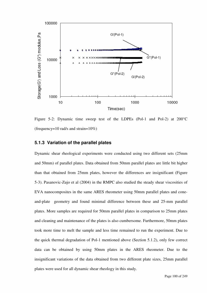
Page 100 of 249
Figure 5-2: Dynamic time sweep test of the LDPEs (Pol-1 and Pol-2) at 200°C
(frequency=10 rad/s and strain=10%)
5.1.3 Variation of the parallel plates
Dynamic shear rheological experiments were conducted using two different sets (25mm
and 50mm) of parallel plates. Data obtained from 50mm parallel plates are little bit higher
than that obtained from 25mm plates, however the differences are insignificant (Figure
5-3). Pasanovic-Zujo et al (2004) in the RMPC also studied the steady shear viscosities of
EVA nanocomposites in the same ARES rheometer using 50mm parallel plates and cone-
and-plate geometry and found minimal difference between these and 25-mm parallel
plates. More samples are required for 50mm parallel plates in comparison to 25mm plates
and cleaning and maintenance of the plates is also cumbersome. Furthermore, 50mm plates
took more time to melt the sample and less time remained to run the experiment. Due to
the quick thermal degradation of Pol-1 mentioned above (Section 5.1.2), only few correct
data can be obtained by using 50mm plates in the ARES rheometer. Due to the
insignificant variations of the data obtained from two different plate sizes, 25mm parallel
plates were used for all dynamic shear rheology in this study.
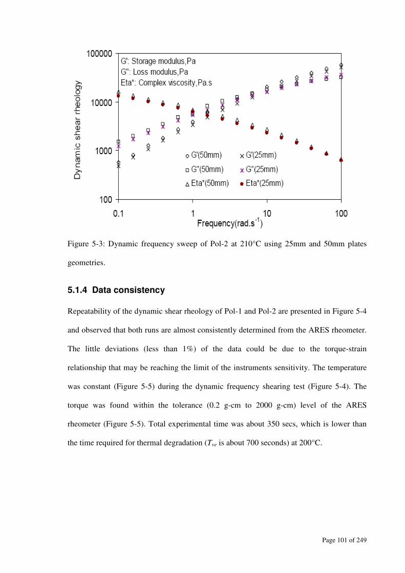
Page 101 of 249
Figure 5-3: Dynamic frequency sweep of Pol-2 at 210°C using 25mm and 50mm plates
geometries.
5.1.4 Data consistency
Repeatability of the dynamic shear rheology of Pol-1 and Pol-2 are presented in Figure 5-4
and observed that both runs are almost consistently determined from the ARES rheometer.
The little deviations (less than 1%) of the data could be due to the torque-strain
relationship that may be reaching the limit of the instruments sensitivity. The temperature
was constant (Figure 5-5) during the dynamic frequency shearing test (Figure 5-4). The
torque was found within the tolerance (0.2 g-cm to 2000 g-cm) level of the ARES
rheometer (Figure 5-5). Total experimental time was about 350 secs, which is lower than
the time required for thermal degradation (Tve is about 700 seconds) at 200°C.
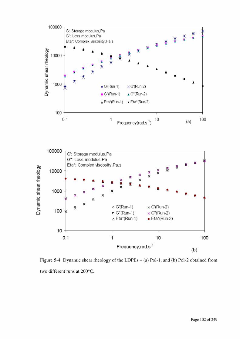
Page 102 of 249
Figure 5-4: Dynamic shear rheology of the LDPEs – (a) Pol-1, and (b) Pol-2 obtained from
two different runs at 200°C.
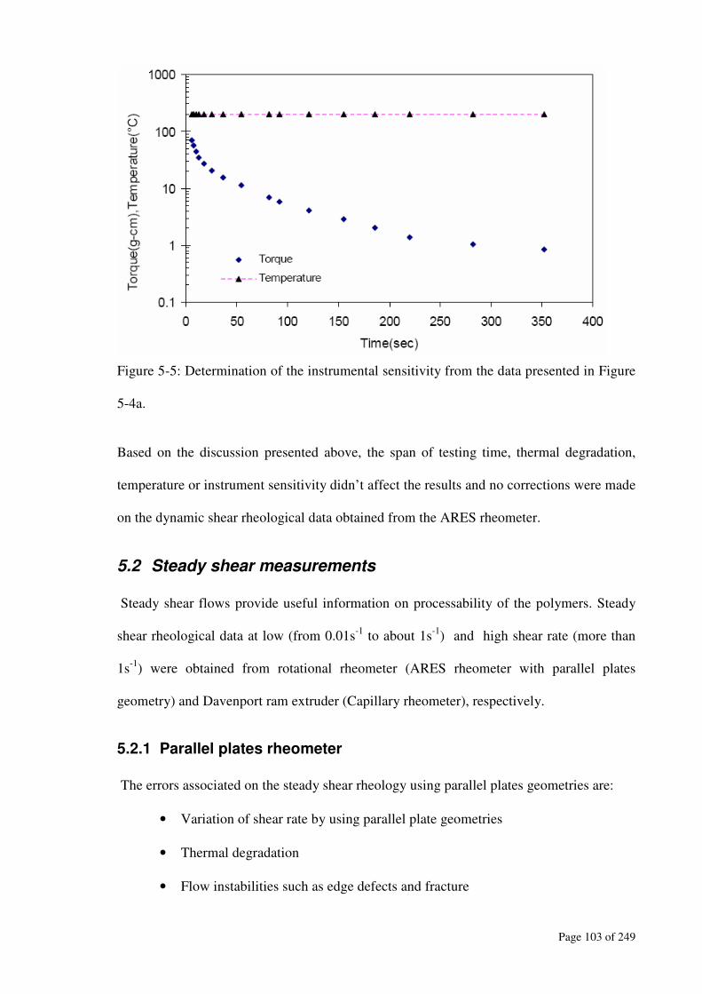
Page 103 of 249
Figure 5-5: Determination of the instrumental sensitivity from the data presented in Figure
5-4a.
Based on the discussion presented above, the span of testing time, thermal degradation,
temperature or instrument sensitivity didn’t affect the results and no corrections were made
on the dynamic shear rheological data obtained from the ARES rheometer.
5.2 Steady shear measurements
Steady shear flows provide useful information on processability of the polymers. Steady
shear rheological data at low (from 0.01s-1
to about 1s-1
) and high shear rate (more than
1s-1
) were obtained from rotational rheometer (ARES rheometer with parallel plates
geometry) and Davenport ram extruder (Capillary rheometer), respectively.
5.2.1 Parallel plates rheometer
The errors associated on the steady shear rheology using parallel plates geometries are:
• Variation of shear rate by using parallel plate geometries
• Thermal degradation
• Flow instabilities such as edge defects and fracture

Page 104 of 249
5.2.1.1 Variation of shear rate
Parallel plate geometry has a deficiency in that the shear rates are not constant along the
radial position of the sample. The variation of shear rate for parallel plates is described by
Equation 5-1.
h
r
r
Ω=γɺ (5-1)
( )
+=
γγπη
ɺɺ dIn
dInM
r
Mr 3
23
(5-2)
where ( )rη = steady shear viscosity at the rim of the plates, Ω = angular velocity, M =
total measured torque, r = radius of the plate at the rim or edge, h = gap between the
plates.
In parallel plate geometry, shear rates range from zero at the centre to maximum at the
edge or rim of the plate. Strain has also been reported to change in a similar manner
(Macosko, 1994, Morrison, 2001). Depending on the range of shear rates, this might cause
a significant error on the measured values. However, a derivative relating the shear stress
to total torque can be used to correct the viscosity obtained from the parallel plate
rheometer (Macosko, 1994). Using the basic expression of viscosity being a ratio of shear
stress to shear rate and Equation 5-2, a corrected version of shear viscosity was determined
in this research and presented in Figure 5-6. Data obtained from steady rate sweep test in
ARES rheometer for a shear rate range of 0.024s-1
to 0.379s-1
, an insignificant variation
was observed between corrected and uncorrected steady shear viscosity (Figure 5-6).

Page 105 of 249
Figure 5-6: Viscosity correction of Pol-1 data (obtained at 200°C from ARES rheometer)
using Equation 5-2.
5.2.1.2 Thermal degradation
The effect of thermal degradation already discussed in the preceding section (5.1.2) of this
chapter. Although steady shear viscosity experiments took a shorter time in comparison to
oscillatory tests (Prasad, 2004), Pol-1 requires a longer time for shear rates higher than
0.1s-1
. The time taken for Pol-1 by the steady rate sweep test (Figure 5-6) is presented in
Figure 5-7. Time sweep runs (Figure 5-2) analysed in the previous section (5.1.2) advised
that traditional steady rate sweep test (rheological data for a certain shear rate range
presented in Figure 5-7) is not suitable for Pol-1 at shear rates higher than 0.1s-1
due to its
quick thermal degradation (Tve is higher than 700s). Unlike steady rate sweep test, step rate
test in transient mode of ARES rheometer took short time to determine the viscosity at a
particular shear rate. The disadvantages of step rate test are that it needs more material and
a longer time to get a flow curve (viscosity versus shear rate) in comparison to steady rate
sweep test.
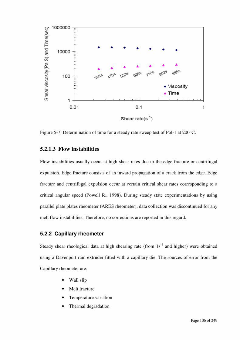
Page 106 of 249
Figure 5-7: Determination of time for a steady rate sweep test of Pol-1 at 200°C.
5.2.1.3 Flow instabilities
Flow instabilities usually occur at high shear rates due to the edge fracture or centrifugal
expulsion. Edge fracture consists of an inward propagation of a crack from the edge. Edge
fracture and centrifugal expulsion occur at certain critical shear rates corresponding to a
critical angular speed (Powell R., 1998). During steady state experimentations by using
parallel plate plates rheometer (ARES rheometer), data collection was discontinued for any
melt flow instabilities. Therefore, no corrections are reported in this regard.
5.2.2 Capillary rheometer
Steady shear rheological data at high shearing rate (from 1s-1
and higher) were obtained
using a Davenport ram extruder fitted with a capillary die. The sources of error from the
Capillary rheometer are:
• Wall slip
• Melt fracture
• Temperature variation
• Thermal degradation
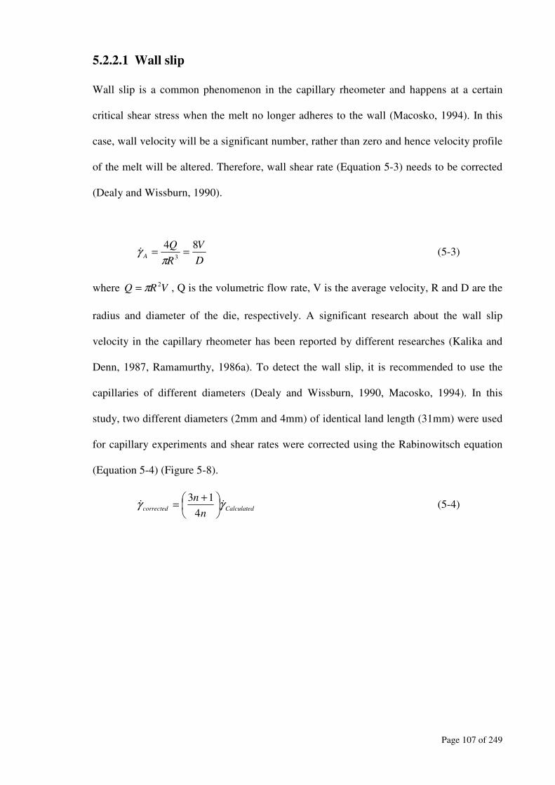
Page 107 of 249
5.2.2.1 Wall slip
Wall slip is a common phenomenon in the capillary rheometer and happens at a certain
critical shear stress when the melt no longer adheres to the wall (Macosko, 1994). In this
case, wall velocity will be a significant number, rather than zero and hence velocity profile
of the melt will be altered. Therefore, wall shear rate (Equation 5-3) needs to be corrected
(Dealy and Wissburn, 1990).
D
V
R
Q
A
843
==π
γɺ (5-3)
where VRQ2π= , Q is the volumetric flow rate, V is the average velocity, R and D are the
radius and diameter of the die, respectively. A significant research about the wall slip
velocity in the capillary rheometer has been reported by different researches (Kalika and
Denn, 1987, Ramamurthy, 1986a). To detect the wall slip, it is recommended to use the
capillaries of different diameters (Dealy and Wissburn, 1990, Macosko, 1994). In this
study, two different diameters (2mm and 4mm) of identical land length (31mm) were used
for capillary experiments and shear rates were corrected using the Rabinowitsch equation
(Equation 5-4) (Figure 5-8).
Calculatedcorrected
n
nγγ ɺɺ
+=
4
13 (5-4)
Page 108 of 249
Figure 5-8: Correction of Capillary rheometer data of Pol-1 obtained at 190°C.
5.2.2.2 Melt fracture
Melt fracture limits the shear stress for highly viscous material and usually happens at a
critical shear stress of about 100kPa (Macosko, 1994). This shear stress limitation was
maintained to avoid any possible error from the capillary experiments. Any discolorations
of the extrudate strand or abnormal data from the transducer were considered as an
erroneous data due to thermal degradation or other reasons. The last data presented in
Figure 5-9 showed a shear stress of 102kPa at a shear rate of 36.07s-1
.
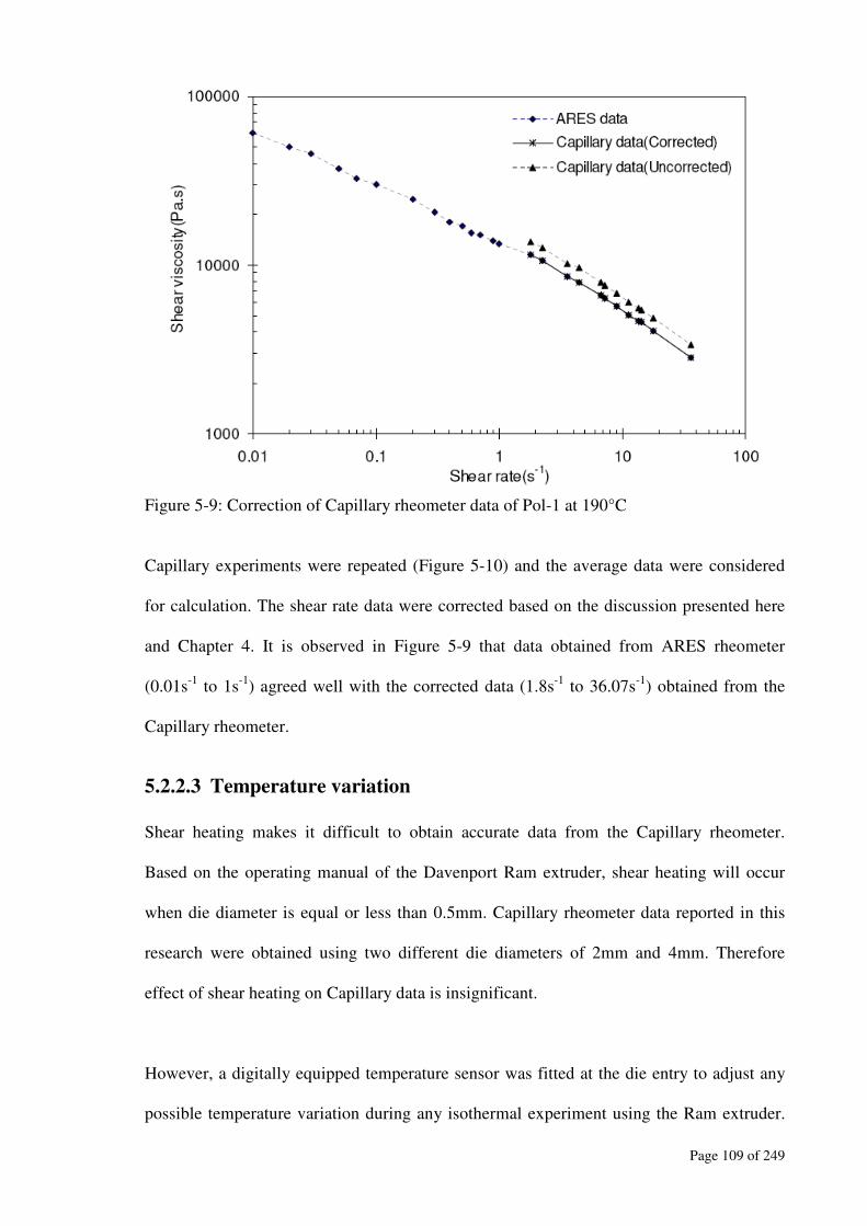
Page 109 of 249
Figure 5-9: Correction of Capillary rheometer data of Pol-1 at 190°C
Capillary experiments were repeated (Figure 5-10) and the average data were considered
for calculation. The shear rate data were corrected based on the discussion presented here
and Chapter 4. It is observed in Figure 5-9 that data obtained from ARES rheometer
(0.01s-1
to 1s-1
) agreed well with the corrected data (1.8s-1
to 36.07s-1
) obtained from the
Capillary rheometer.
5.2.2.3 Temperature variation
Shear heating makes it difficult to obtain accurate data from the Capillary rheometer.
Based on the operating manual of the Davenport Ram extruder, shear heating will occur
when die diameter is equal or less than 0.5mm. Capillary rheometer data reported in this
research were obtained using two different die diameters of 2mm and 4mm. Therefore
effect of shear heating on Capillary data is insignificant.
However, a digitally equipped temperature sensor was fitted at the die entry to adjust any
possible temperature variation during any isothermal experiment using the Ram extruder.
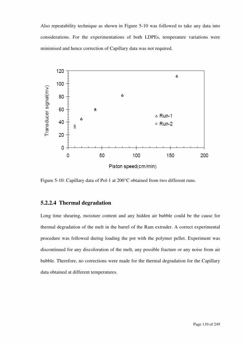
Page 110 of 249
Also repeatability technique as shown in Figure 5-10 was followed to take any data into
considerations. For the experimentations of both LDPEs, temperature variations were
minimised and hence correction of Capillary data was not required.
Figure 5-10: Capillary data of Pol-1 at 200°C obtained from two different runs.
5.2.2.4 Thermal degradation
Long time shearing, moisture content and any hidden air bubble could be the cause for
thermal degradation of the melt in the barrel of the Ram extruder. A correct experimental
procedure was followed during loading the pot with the polymer pellet. Experiment was
discontinued for any discoloration of the melt, any possible fracture or any noise from air
bubble. Therefore, no corrections were made for the thermal degradation for the Capillary
data obtained at different temperatures.

Page 111 of 249
5.3 Extensional rheological measurement
Uniaxial extension is very sensitive to macromolecular and microstructural factors relevant
to blown film process. Extensional rheological studies were carried out with a constant
strain rate stretching experiments using RME rheometer. The common errors that need to
be accounted for the RME rheometer experiment are:
• Temperature gradients
• Inhomogeneity of the sample
• Time delay in the measurement
• Force deviation
5.3.1 Time delay
Based on the methodology described Chapters 2 and 4, stress and void free plaques were
prepared for use in the RME experiments. Several factors may cause a time delay during
the test, which usually occurs in the first tenths of a second after starting the test. As
mentioned by Schulze et al (2001) backlash in the gearing system of the belt’s motor may
be the reason for this time delay. During different runs of this RME study, a time delay of
0.1 second was identified at all stretching rates caused by backlash (Figure 5-11). This
value of time delay (0.1second) was constant in all runs and didn’t have any significant
effect when extensional data of the two LDPEs were compared.
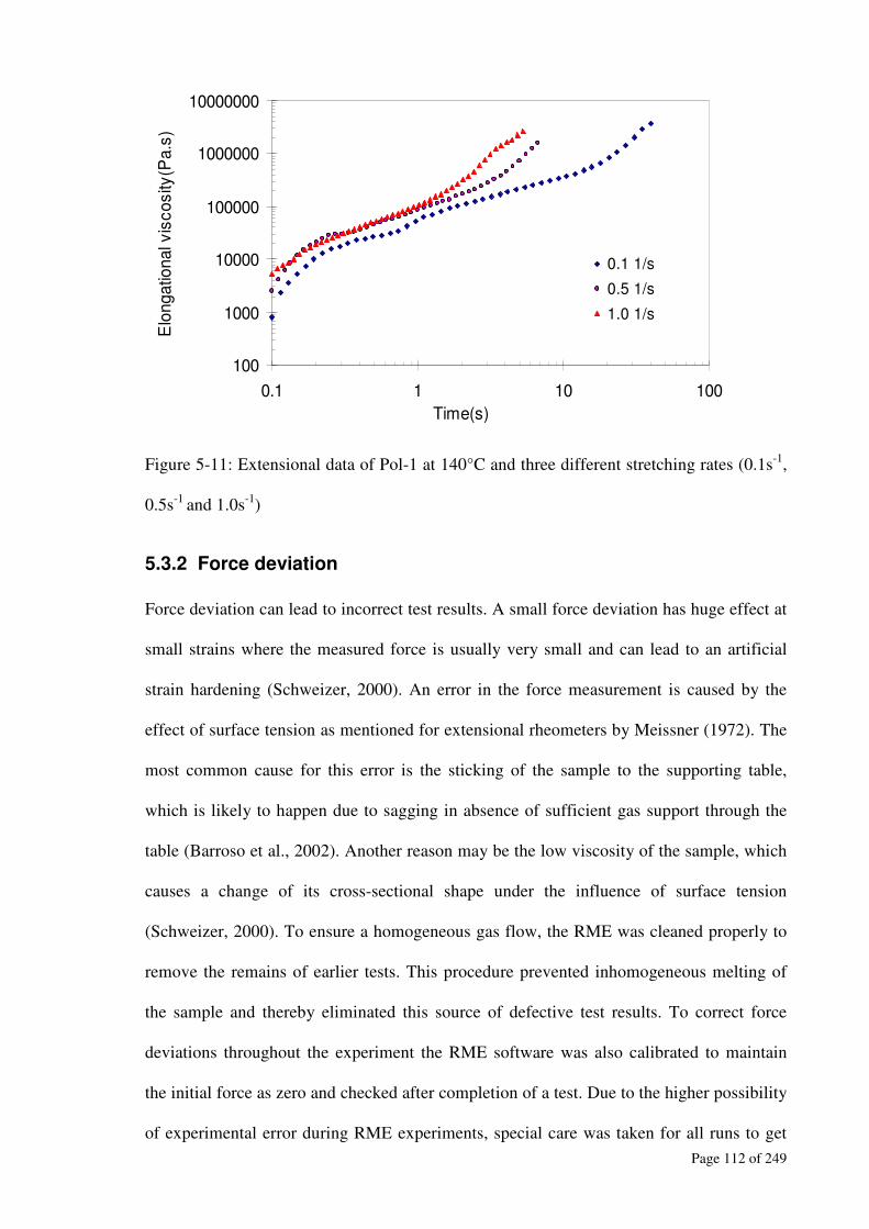
Page 112 of 249
100
1000
10000
100000
1000000
10000000
0.1 1 10 100
Time(s)
Elo
ngatio
nal v
iscosity
(Pa.s
)
0.1 1/s
0.5 1/s
1.0 1/s
Figure 5-11: Extensional data of Pol-1 at 140°C and three different stretching rates (0.1s-1
,
0.5s-1
and 1.0s-1
)
5.3.2 Force deviation
Force deviation can lead to incorrect test results. A small force deviation has huge effect at
small strains where the measured force is usually very small and can lead to an artificial
strain hardening (Schweizer, 2000). An error in the force measurement is caused by the
effect of surface tension as mentioned for extensional rheometers by Meissner (1972). The
most common cause for this error is the sticking of the sample to the supporting table,
which is likely to happen due to sagging in absence of sufficient gas support through the
table (Barroso et al., 2002). Another reason may be the low viscosity of the sample, which
causes a change of its cross-sectional shape under the influence of surface tension
(Schweizer, 2000). To ensure a homogeneous gas flow, the RME was cleaned properly to
remove the remains of earlier tests. This procedure prevented inhomogeneous melting of
the sample and thereby eliminated this source of defective test results. To correct force
deviations throughout the experiment the RME software was also calibrated to maintain
the initial force as zero and checked after completion of a test. Due to the higher possibility
of experimental error during RME experiments, special care was taken for all runs to get

Page 113 of 249
the best values of the data. A comparison of the force data obtained from two different
RME runs at a stretching rate of 1.0s-1
is presented in Figure 5-1. The force deviation is
observed to be insignificant between runs.
0
20
40
60
80
100
120
0 1 2 3 4 5 6
Time(sec)
Forc
e(C
N)
Run-1 Run-2
Figure 5-12: Comparison of extensional data (stretching rate=1.0s-1
) of Pol-1 at 140°C.
Viscosity of Pol-2 is lower than Pol-1 and to avoid any possible error regarding force
deviation or samples inhomogeneity, extensional viscosity data of both polymers were
obtained at lower temperatures (140°C, 150°C and 170°C). Due to the insignificant force
deviations and time delay observed during experimental runs, RME data didn’t require any
correction.
5.4 WAXD study
The error accounted in WAXD study is generally the effect of X-Ray scattering by air
(Alexander, 1969). This effect is usually corrected by conducting the X-Ray experiments
in a vacuum condition. Cser and Bhattacharya (2003) corrected the sample WAXD
intensities by subtracting the background scattering generated by air. However, this effect
is less significant and can easily be ignored for diffraction angle(2θ) of 1.6 or higher

Page 114 of 249
(Prasad, 2004). In this study, the WAXD peaks and widths were analyzed and found
between diffraction angle (2θ) of 10° and 30°. Therefore, no corrections were made on any
data obtained from the Phillips X-Ray generator (Philips PW 1130, Holland). Moreover, a
reasonable agreement has been observed between two different WAXD runs as shown in
Figure 5-13.
0
100
200
300
400
500
600
15 16 17 18 19 20 21 22 23 24 25
Diffraction angle(2θ)
Inte
ns
ity
Run-1
Run-2
Figure 5-13: WAXD study of Pol-1 film in MD obtained at die temperature=200°C and
blower setting=2.6.

Page 115 of 249
CHAPTER : 6
Results and Discussion of Rheological, Thermal, and Crystalline Properties
Molecular, rheological, thermal and crystalline properties are presented in this chapter. The
viscoelastic properties of the LDPEs (Pol-1 and Pol-2) will be discussed here in terms their
molecular structures. Determination of the melt relaxation time, zero shear viscosity and
flow activation energy has been reported here in detail. These rheological data will be used
in the blown film simulation presented in Chapter 7. Wide angle X-Ray diffraction
(WAXD) data will be analysed to discuss the morphology and crystalline properties of the
blown film obtained at different cooling rates. Modulated differential scanning calorimetric
(MDSC) data will be used for thermal analysis and to discuss the effect of molecular
structure on the crystallinity of the LDPEs and their blown film.
6.1 Molecular properties of the LDPEs
The molecular structure of the LDPE (branched chain polymers) has a significant effect on
the melt rheology, processing and the end product. Generally, short chain branching of
LDPE influences the morphology and solid state properties, whereas long chain branching
(LCB) has a major effect on melt rheology. Different grades of LDPEs are used for
different applications and it is essential for the film producer to process similar polymers to
maintain the consistency as per customer requirements. It is challenging sometimes for the
film producer to maintain that consistency of the end product properties. It is well known
that depending on the resin manufacturing conditions (i.e., pressure and temperature of the
reaction or types of catalyst), molecular structures of the LDPEs may vary even though
produced from the same reactor and manufacturer. Therefore, it is vital to study the
molecular structure of the LDPEs before they are considered for processing.
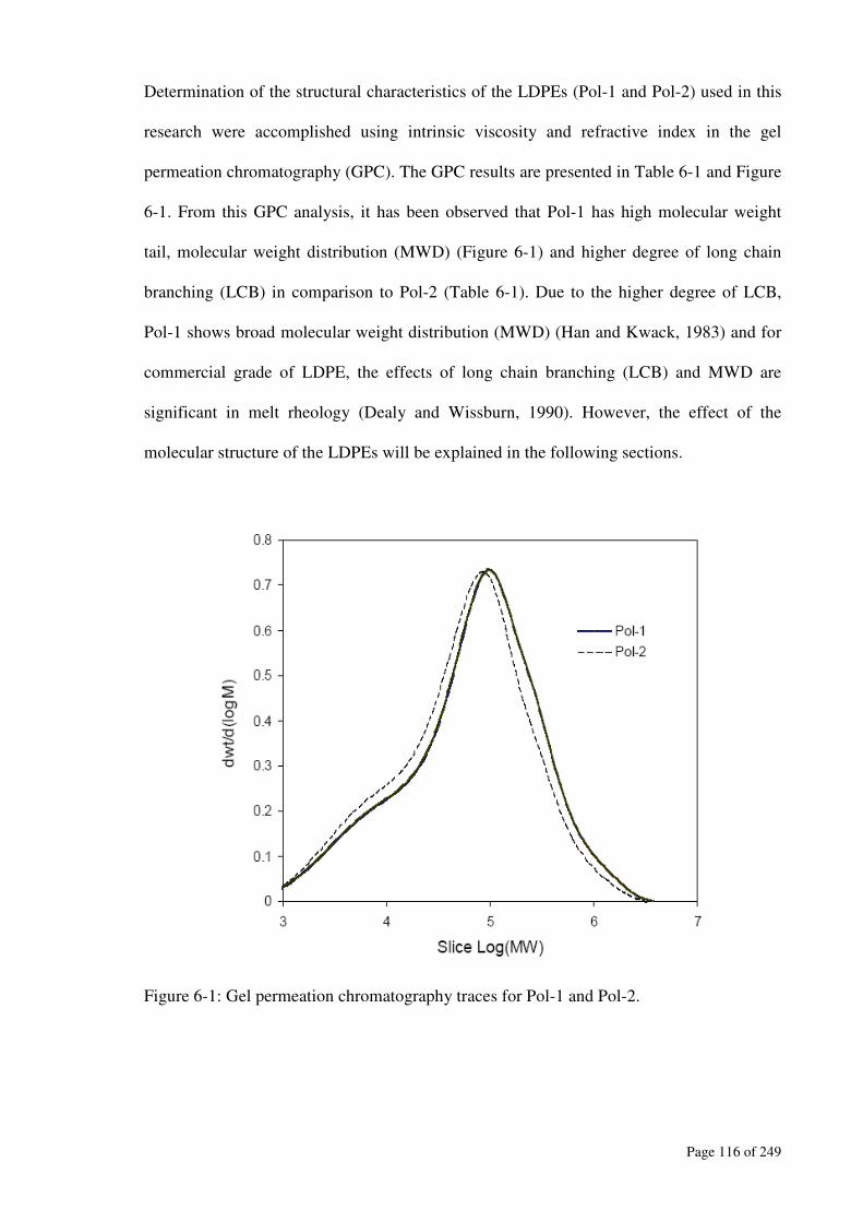
Page 116 of 249
Determination of the structural characteristics of the LDPEs (Pol-1 and Pol-2) used in this
research were accomplished using intrinsic viscosity and refractive index in the gel
permeation chromatography (GPC). The GPC results are presented in Table 6-1 and Figure
6-1. From this GPC analysis, it has been observed that Pol-1 has high molecular weight
tail, molecular weight distribution (MWD) (Figure 6-1) and higher degree of long chain
branching (LCB) in comparison to Pol-2 (Table 6-1). Due to the higher degree of LCB,
Pol-1 shows broad molecular weight distribution (MWD) (Han and Kwack, 1983) and for
commercial grade of LDPE, the effects of long chain branching (LCB) and MWD are
significant in melt rheology (Dealy and Wissburn, 1990). However, the effect of the
molecular structure of the LDPEs will be explained in the following sections.
Figure 6-1: Gel permeation chromatography traces for Pol-1 and Pol-2.
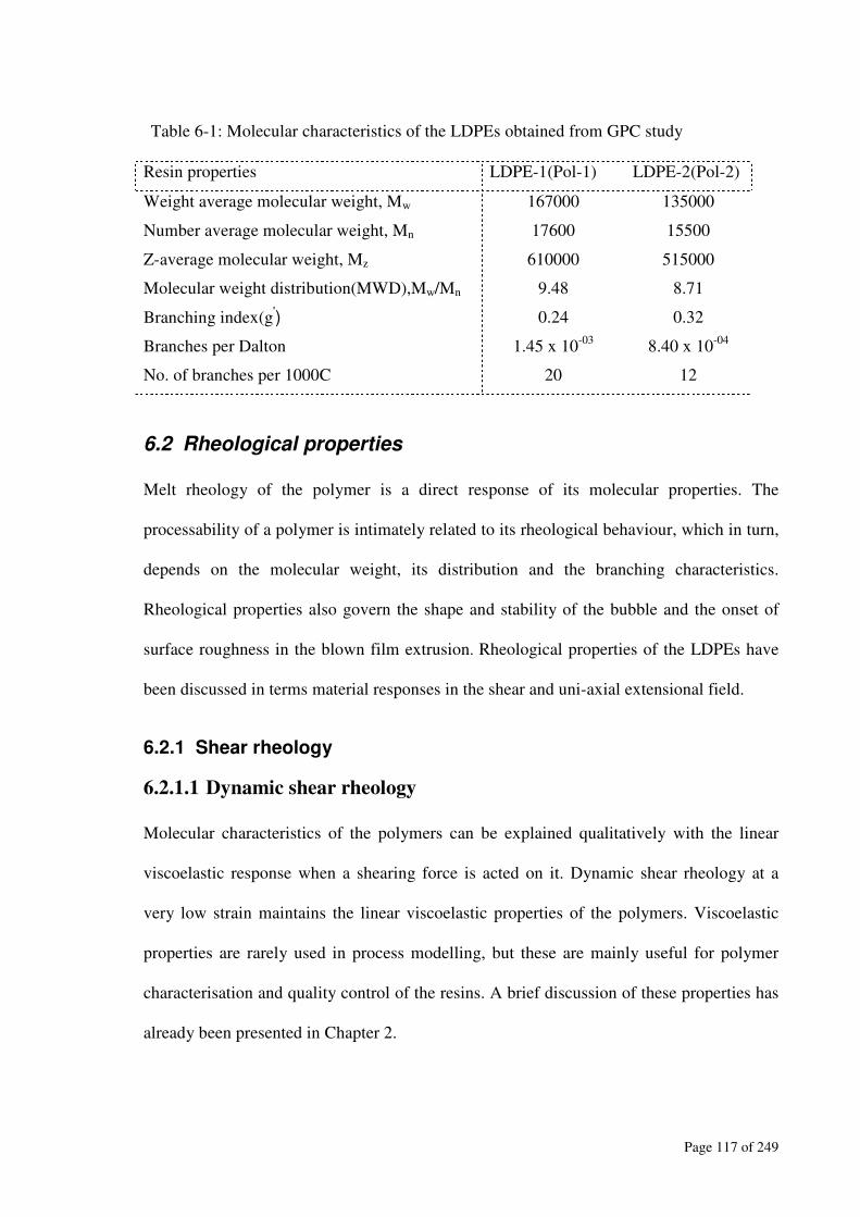
Page 117 of 249
Table 6-1: Molecular characteristics of the LDPEs obtained from GPC study
Resin properties LDPE-1(Pol-1) LDPE-2(Pol-2)
Weight average molecular weight, Mw 167000 135000
Number average molecular weight, Mn 17600 15500
Z-average molecular weight, Mz 610000 515000
Molecular weight distribution(MWD),Mw/Mn 9.48 8.71
Branching index(g') 0.24 0.32
Branches per Dalton 1.45 x 10-03
8.40 x 10-04
No. of branches per 1000C 20 12
6.2 Rheological properties
Melt rheology of the polymer is a direct response of its molecular properties. The
processability of a polymer is intimately related to its rheological behaviour, which in turn,
depends on the molecular weight, its distribution and the branching characteristics.
Rheological properties also govern the shape and stability of the bubble and the onset of
surface roughness in the blown film extrusion. Rheological properties of the LDPEs have
been discussed in terms material responses in the shear and uni-axial extensional field.
6.2.1 Shear rheology
6.2.1.1 Dynamic shear rheology
Molecular characteristics of the polymers can be explained qualitatively with the linear
viscoelastic response when a shearing force is acted on it. Dynamic shear rheology at a
very low strain maintains the linear viscoelastic properties of the polymers. Viscoelastic
properties are rarely used in process modelling, but these are mainly useful for polymer
characterisation and quality control of the resins. A brief discussion of these properties has
already been presented in Chapter 2.

Page 118 of 249
6.2.1.1.1 Effect of short chain branching
Determination of the effect of branching on melt rheology, thermal and crystalline
properties is a focus of this study. Therefore, it is essential to determine whether long or
short chain branching are dominating those properties mentioned above. For commercial
grades of LDPE, the effects of long chain branching (LCB) on melt rheology are
accompanied with the MWD (Dealy and Wissburn, 1990). Effect of LCB on melt rheology
has also been reported by others (Foster et al., 1980b, Graessley, 1982, Wagner, 2006,
Wood-Adams et al., 2000, Majumder et al., 2007a). The effect of short chain branching
(SCB) on melt rheology can be determined by plotting Mw independent data of η*/η0
versus ωη0 (Wood-Adams et al., 2000) and presented here for the proposed LDPEs (Figure
6-2). The effect of Mw has been avoided by shifting complex viscosity data on both axes
using the viscosity at low shear (Figure 6-2). Another study regarding the effect of short
chain branching was reported following the approach of Booij and Palmen (1982) using a
Mw independent plot of phase (loss) angle against the product of the zero shear viscosity
and frequency (Figure 6-3). From these two different analyses (Figure 6-2 and Figure 6-3)
of the LDPEs, a small variation between the polymers (Pol-1 and Pol-2) has been
observed. Therefore, the effect of SCB of Pol-1 and Pol-2 is insignificant on their linear
viscoelastic properties considered in this study. The phase angle in Figure 6-3 also
indicates that the rheological data at low shear rate didn’t represent the data at the terminal
zone. It was not possible to obtain the data at the terminal zone for both polymers. This
was due to the long time requirements to obtain the data at very low shear rate where
thermal degradation (discussed in Chapters 4 and 5) of the polymers interrupted the results.
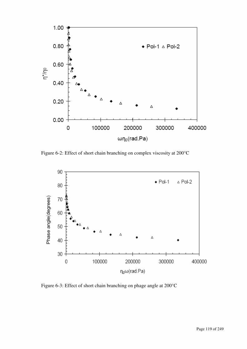
Page 119 of 249
Figure 6-2: Effect of short chain branching on complex viscosity at 200°C
Figure 6-3: Effect of short chain branching on phage angle at 200°C
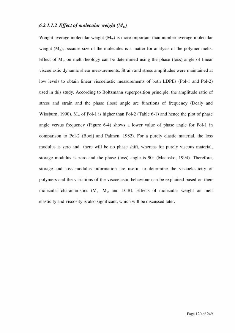
Page 120 of 249
6.2.1.1.2 Effect of molecular weight (Mw)
Weight average molecular weight (Mw) is more important than number average molecular
weight (Mn), because size of the molecules is a matter for analysis of the polymer melts.
Effect of Mw on melt rheology can be determined using the phase (loss) angle of linear
viscoelastic dynamic shear measurements. Strain and stress amplitudes were maintained at
low levels to obtain linear viscoelastic measurements of both LDPEs (Pol-1 and Pol-2)
used in this study. According to Boltzmann superposition principle, the amplitude ratio of
stress and strain and the phase (loss) angle are functions of frequency (Dealy and
Wissburn, 1990). Mw of Pol-1 is higher than Pol-2 (Table 6-1) and hence the plot of phase
angle versus frequency (Figure 6-4) shows a lower value of phase angle for Pol-1 in
comparison to Pol-2 (Booij and Palmen, 1982). For a purely elastic material, the loss
modulus is zero and there will be no phase shift, whereas for purely viscous material,
storage modulus is zero and the phase (loss) angle is 90° (Macosko, 1994). Therefore,
storage and loss modulus information are useful to determine the viscoelasticity of
polymers and the variations of the viscoelastic behaviour can be explained based on their
molecular characteristics (Mn, Mw and LCB). Effects of molecular weight on melt
elasticity and viscosity is also significant, which will be discussed later.
Page 121 of 249
Figure 6-4: Phase angle of Pol-1 and Pol-2 as a function of frequency obtained at 200°C.
6.2.1.1.3 Linear viscoelastic properties of the LDPEs
Dynamic shear rheological properties of the LDPEs at 200°C have been presented in
Figure 6-5 and a significant variation of rheological response due to their different
molecular structure was observed. In all cases, Pol-1 was found to have higher storage
modulus (G’), loss modulus (G”) and complex viscosity (η*) than Pol-2 except the
crossover frequency. Therefore, Pol-1 is more viscoelastic than Pol-2 due to its higher
value of Mw and higher degree of LCB. Higher value of Mw and LCB of Pol-1 will also
enhance the molecular entanglements at a lower shear rate and hence higher zero shear
viscosity.
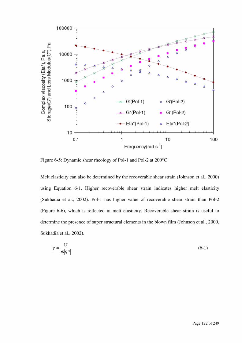
Page 122 of 249
Figure 6-5: Dynamic shear rheology of Pol-1 and Pol-2 at 200°C
Melt elasticity can also be determined by the recoverable shear strain (Johnson et al., 2000)
using Equation 6-1. Higher recoverable shear strain indicates higher melt elasticity
(Sukhadia et al., 2002). Pol-1 has higher value of recoverable shear strain than Pol-2
(Figure 6-6), which is reflected in melt elasticity. Recoverable shear strain is useful to
determine the presence of super structural elements in the blown film (Johnson et al., 2000,
Sukhadia et al., 2002).
*
'
ηωγ
G≈ (6-1)

Page 123 of 249
Figure 6-6: Recoverable shear strain of Pol-1 and Pol-2 at 200°C
From the GPC analysis it is found that Pol-1 has more branches than Pol-2 (Table 6-1),
which means that according to past study (Nielson and Landel, 1993) , Pol-1 should show
lower viscosity than Pol-2. In this research, it shows that Pol-1 has higher viscosity than
Pol-2 at low shear rate. Pol-1 also has higher degree of shear thinning in comparison to
Pol-2 at high shear rate (Figure 6-5) due to its possible lower value of radius of gyration
for higher degree of LCB, producing fewer entanglements and a lower viscosity (Macosko,
1994, Majumder et al., 2007a, Dealy and Wissburn, 1990). There are a number of
situations in polymer processing where extruder operation is interrupted (or turned off) due
to the viscosity of the polymers being processed (Micic and Bhattacharya, 2000,
Rauwendaal, 1985). In those situations, extra power is required by the extruder motor to
process those polymers. Therefore, higher shear thinning behaviour along with suitable
melt strength are desirable at higher extrusion rates in the film blowing process of the
LDPE for a continuous production. Crossover frequency of Pol-1 was found to be lower
Page 124 of 249
than that for Pol-2 (Figure 6-5), which indicates the higher characteristic relaxation time of
Pol-1 than Pol-2.
6.2.1.2 Zero shear viscosity (ZSV)
For blown film simulation, it is essential to determine the zero shear viscosity (ZSV). In
the melt flow curve (viscosity versus shear rate), a Newtonian plateau at very low shear
rate is usually considered as the ZSV. For polymers of very low molecular weight, this
ZSV can be obtained directly from the shearing experiment. However, this is really
difficult to obtain for high Mw polymers. From the experimental data presented in Figure
6-7, it was impossible to determine the ZSV, since there was no distinct plateau detected at
a lower shear rate of 0.01s-1
. Therefore, a modified Cross model (Equation 6-2) was used
to determine the zero shear viscosity (Table 6-2 and 6-3) of the LDPEs. Data from ARES
and Capillary rheometer were combined to fit into the Cross model predictions (Figure
6-7). The precision of fitting between model predictions and experimental data is also
presented in Table 6-2 and 6-3. For Pol-1, higher value of ZSV resulted from its higher Mw
and higher degree of LCB characteristics as the branch length becomes comparable to
critical molecular weight for entanglement like a linear chain (Han and Kwack, 1983,
Micic and Bhattacharya, 2000, Dealy and Wissburn, 1990). Han and Kwack (1983) also
reported that at low shear rates, higher value of viscosity is related to the weight-average
molecular weight (Mw) and at high shear rates viscosity goes down depending on the
number-average molecular weight (Mn). In this study, this statement is true at low shear
rate (Figure 6-7) but at high shear rate LCB might be responsible for higher shear thinning
sensitivity than number average molecular weight. Viscosity of the resins at any shear rate
can be obtained using the modified Cross model (Equation 6-2) and the parameters are
presented in Table 6-2 and 6-3.
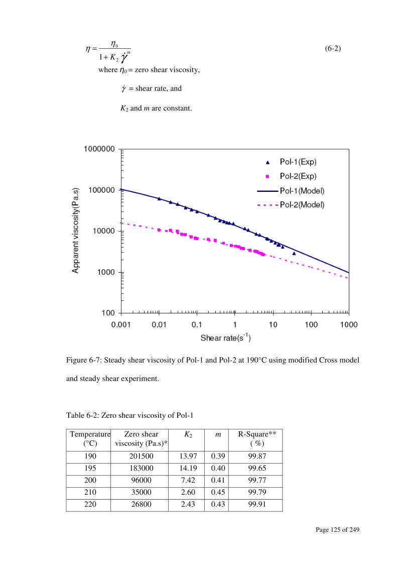
Page 125 of 249
γ
ηη
ɺm
K 2
0
1+= (6-2)
where η0 = zero shear viscosity,
γɺ = shear rate, and
K2 and m are constant.
Figure 6-7: Steady shear viscosity of Pol-1 and Pol-2 at 190°C using modified Cross model
and steady shear experiment.
Table 6-2: Zero shear viscosity of Pol-1
Temperature
(°C)
Zero shear
viscosity (Pa.s)*
K2 m R-Square**
( %)
190 201500 13.97 0.39 99.87
195 183000 14.19 0.40 99.65
200 96000 7.42 0.41 99.77
210 35000 2.60 0.45 99.79
220 26800 2.43 0.43 99.91
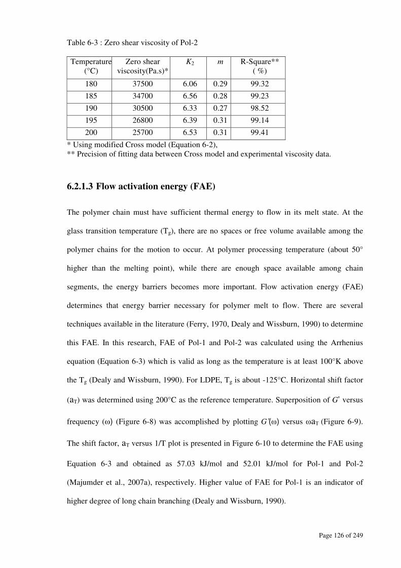
Page 126 of 249
Table 6-3 : Zero shear viscosity of Pol-2
Temperature
(°C)
Zero shear
viscosity(Pa.s)*
K2 m R-Square**
( %)
180 37500 6.06 0.29 99.32
185 34700 6.56 0.28 99.23
190 30500 6.33 0.27 98.52
195 26800 6.39 0.31 99.14
200 25700 6.53 0.31 99.41
* Using modified Cross model (Equation 6-2),
** Precision of fitting data between Cross model and experimental viscosity data.
6.2.1.3 Flow activation energy (FAE)
The polymer chain must have sufficient thermal energy to flow in its melt state. At the
glass transition temperature (Tg), there are no spaces or free volume available among the
polymer chains for the motion to occur. At polymer processing temperature (about 50°
higher than the melting point), while there are enough space available among chain
segments, the energy barriers becomes more important. Flow activation energy (FAE)
determines that energy barrier necessary for polymer melt to flow. There are several
techniques available in the literature (Ferry, 1970, Dealy and Wissburn, 1990) to determine
this FAE. In this research, FAE of Pol-1 and Pol-2 was calculated using the Arrhenius
equation (Equation 6-3) which is valid as long as the temperature is at least 100°K above
the Tg (Dealy and Wissburn, 1990). For LDPE, Tg is about -125°C. Horizontal shift factor
(aT) was determined using 200°C as the reference temperature. Superposition of G’ versus
frequency (ω) (Figure 6-8) was accomplished by plotting G’(ω) versus ωaT (Figure 6-9).
The shift factor, aT versus 1/T plot is presented in Figure 6-10 to determine the FAE using
Equation 6-3 and obtained as 57.03 kJ/mol and 52.01 kJ/mol for Pol-1 and Pol-2
(Majumder et al., 2007a), respectively. Higher value of FAE for Pol-1 is an indicator of
higher degree of long chain branching (Dealy and Wissburn, 1990).
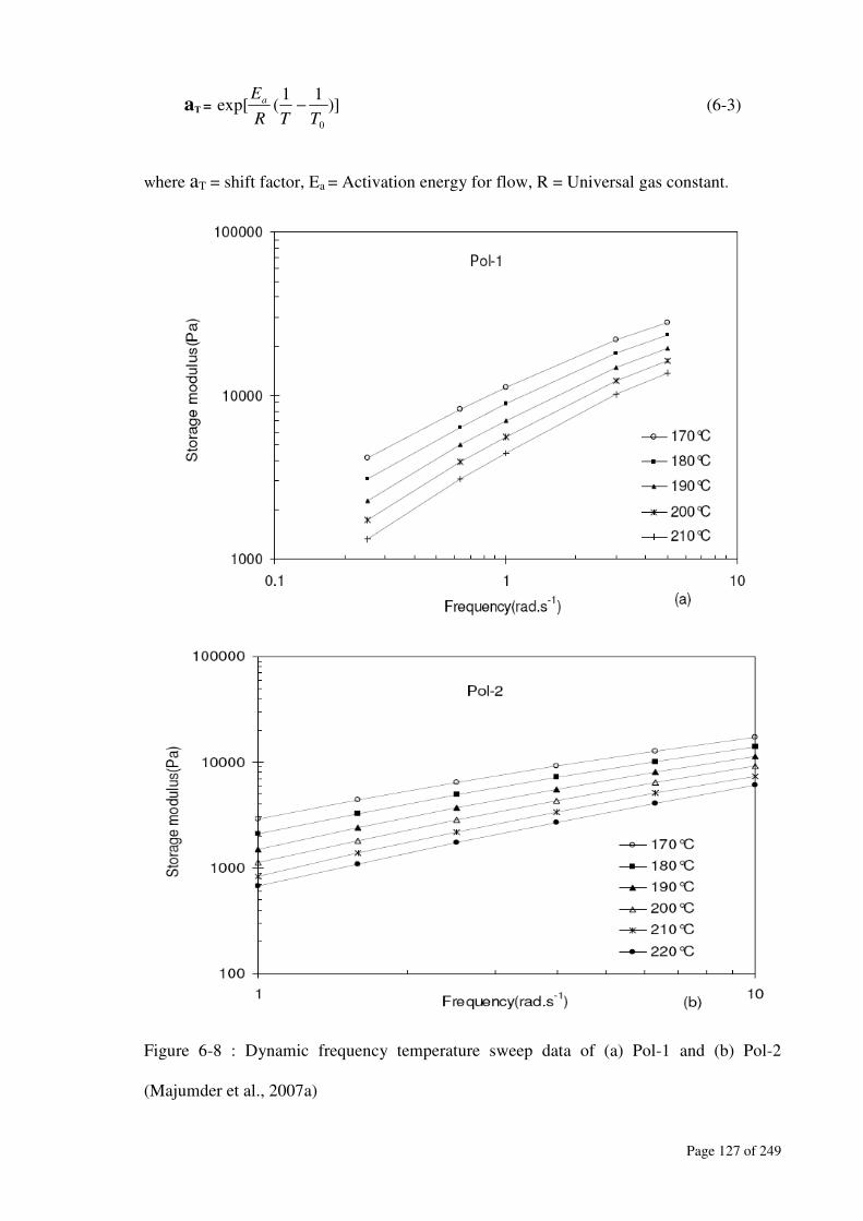
Page 127 of 249
aT = )]11
(exp[0TTR
Ea − (6-3)
where aT = shift factor, Ea = Activation energy for flow, R = Universal gas constant.
Figure 6-8 : Dynamic frequency temperature sweep data of (a) Pol-1 and (b) Pol-2
(Majumder et al., 2007a)
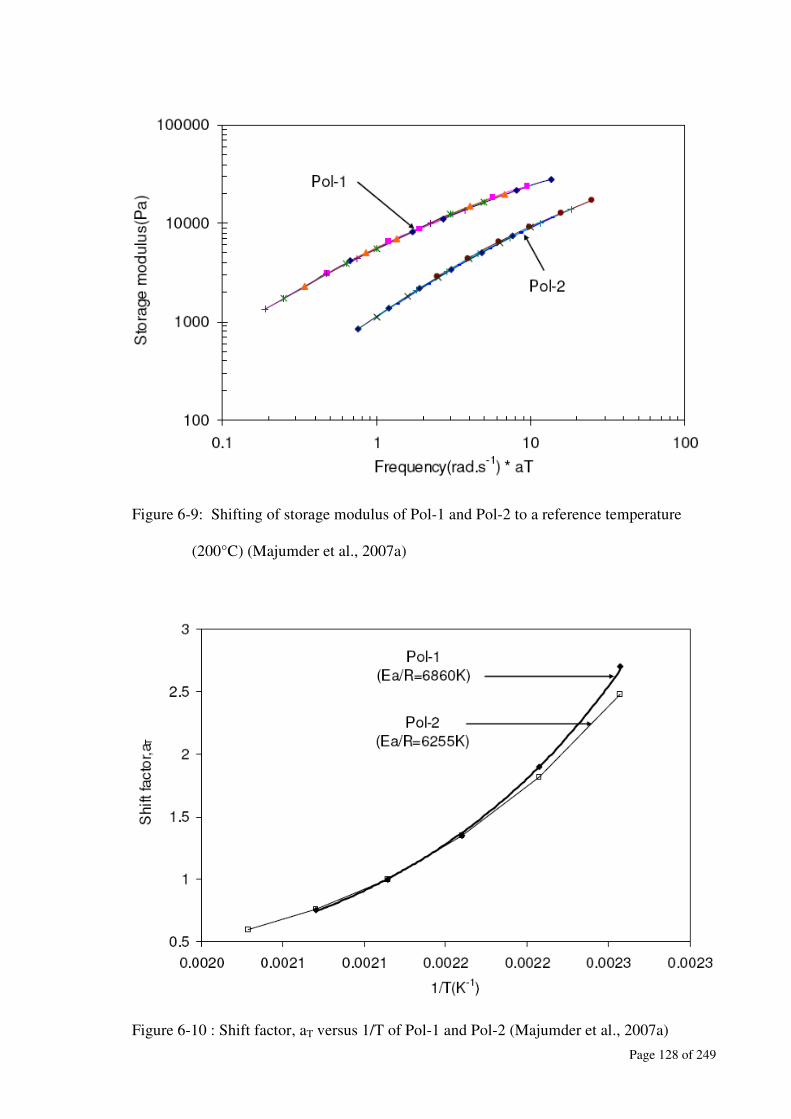
Page 128 of 249
Figure 6-9: Shifting of storage modulus of Pol-1 and Pol-2 to a reference temperature
(200°C) (Majumder et al., 2007a)
Figure 6-10 : Shift factor, aT versus 1/T of Pol-1 and Pol-2 (Majumder et al., 2007a)
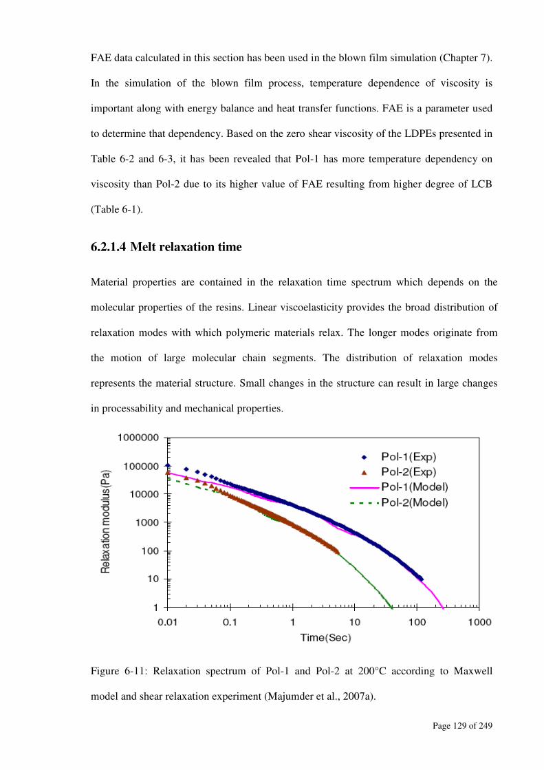
Page 129 of 249
FAE data calculated in this section has been used in the blown film simulation (Chapter 7).
In the simulation of the blown film process, temperature dependence of viscosity is
important along with energy balance and heat transfer functions. FAE is a parameter used
to determine that dependency. Based on the zero shear viscosity of the LDPEs presented in
Table 6-2 and 6-3, it has been revealed that Pol-1 has more temperature dependency on
viscosity than Pol-2 due to its higher value of FAE resulting from higher degree of LCB
(Table 6-1).
6.2.1.4 Melt relaxation time
Material properties are contained in the relaxation time spectrum which depends on the
molecular properties of the resins. Linear viscoelasticity provides the broad distribution of
relaxation modes with which polymeric materials relax. The longer modes originate from
the motion of large molecular chain segments. The distribution of relaxation modes
represents the material structure. Small changes in the structure can result in large changes
in processability and mechanical properties.
Figure 6-11: Relaxation spectrum of Pol-1 and Pol-2 at 200°C according to Maxwell
model and shear relaxation experiment (Majumder et al., 2007a).
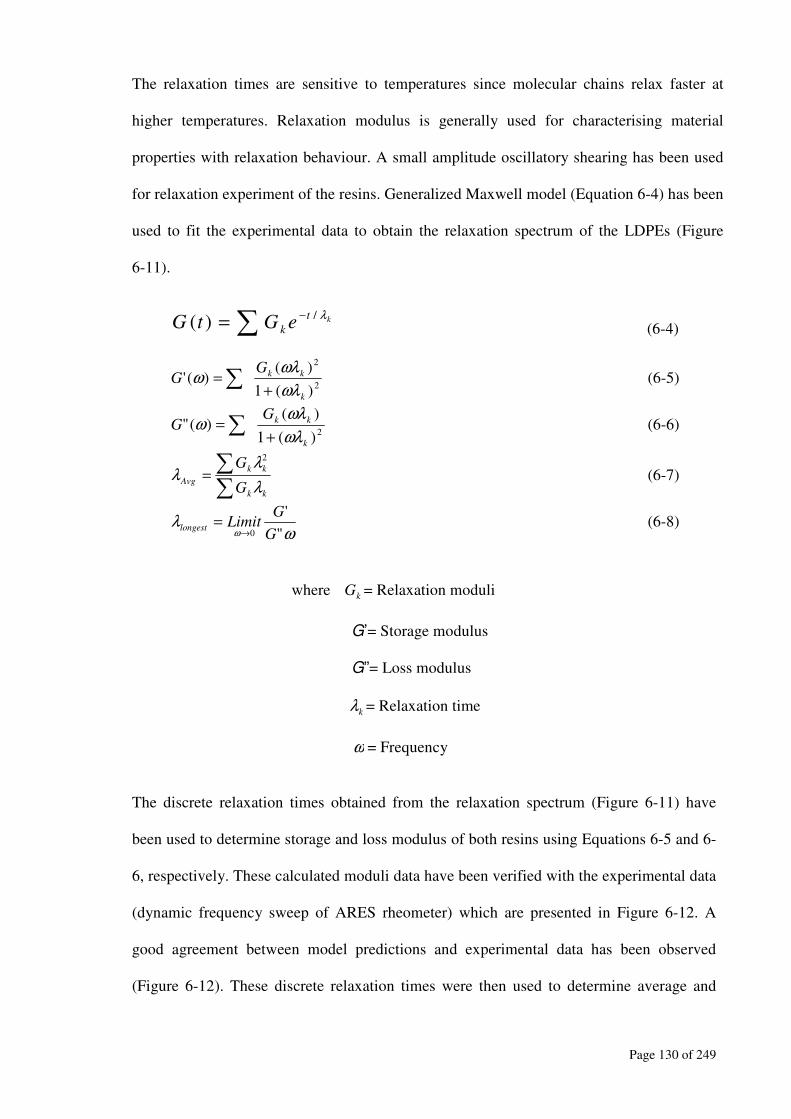
Page 130 of 249
The relaxation times are sensitive to temperatures since molecular chains relax faster at
higher temperatures. Relaxation modulus is generally used for characterising material
properties with relaxation behaviour. A small amplitude oscillatory shearing has been used
for relaxation experiment of the resins. Generalized Maxwell model (Equation 6-4) has been
used to fit the experimental data to obtain the relaxation spectrum of the LDPEs (Figure
6-11).
kt
keGtG
λ/)(
−∑= (6-4)
2
2
)(1
)()('
k
kkG
Gωλ
ωλω
+=∑ (6-5)
2)(1
)()("
k
kkG
Gωλ
ωλω
+=∑ (6-6)
∑∑
=kk
kk
Avg
G
G
λ
λλ
2
(6-7)
ωλ
ω "
'
0 G
GLimit
longest→
= (6-8)
where k
G = Relaxation moduli
G’= Storage modulus
G”= Loss modulus
k
λ = Relaxation time
ω = Frequency
The discrete relaxation times obtained from the relaxation spectrum (Figure 6-11) have
been used to determine storage and loss modulus of both resins using Equations 6-5 and 6-
6, respectively. These calculated moduli data have been verified with the experimental data
(dynamic frequency sweep of ARES rheometer) which are presented in Figure 6-12. A
good agreement between model predictions and experimental data has been observed
(Figure 6-12). These discrete relaxation times were then used to determine average and

Page 131 of 249
longest relaxation times according to Equations 6-7 and 6-8 respectively and shown in
Table 6-4 and Table 6-5.
Figure 6-12: Storage modulus of Pol-1 and Pol-2 using Maxwell model (Equations 6-5 and
6-6) and experimental data (Majumder et al., 2007a).

Page 132 of 249
Based on the relaxation data presented in Table 6-4Table 6-5 and previous study (Wood-
Adams et al., 2000), it is obvious that effect of LCB on melt relaxation time is significant.
This is because, branched molecules are attached at the branch points to at least two other
chains and can not diffuse out independently like a linear chain (Majumder et al., 2005).
Higher MWD of Pol-1 also favours longer relaxation times (Dealy and Wissburn, 1990).
Therefore, it can be said that due to higher degree of LCB along with higher value of Mw,
relaxation time of Pol-1 is higher in comparison to Pol-2. Low molecular weight and lower
branching characteristics of Pol-2 supports for its lower value of melt elasticity (Figure
6-5), zero shear viscosity (Figure 6-7) and relaxation modulus (Figure 6-11).
Table 6-4 : Relaxation time of Pol-1 at different temperatures
Temperature
(°C)
Average Maxwell relaxation
time using Equation 6-7, λ Avg
(Sec)
Longest relaxation time at ω=0.001
rad.s-1
using Equation 6-8, λ longest
(Sec)
190 21.78 21.58
195 17.70 17.53
200 14.65 14.57
210 12.96 12.88
220 11.40 11.41
Table 6-5 : Relaxation time of Pol-2 at different temperatures
Temperature
(°C)
Average Maxwell relaxation
time using Equation 6-7, λ Avg
(Sec)
Longest relaxation time at ω=0.001
rad.s-1
using Equation 6-8, λ longest
(Sec)
180 3.80 3.80
185 2.89 2.89
190 2.34 2.30
195 2.09 2.11
200 1.74 1.74
Relaxation time has an important role in the blown film process and its simulation. Effect of
melt relaxation is significant in the solidification and crystallizations of the polymer chains
during biaxial stretching and orientation, which ultimately influence the morphology and
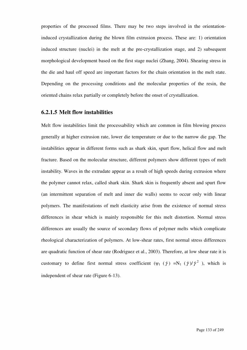
Page 133 of 249
properties of the processed films. There may be two steps involved in the orientation-
induced crystallization during the blown film extrusion process. These are: 1) orientation
induced structure (nuclei) in the melt at the pre-crystallization stage, and 2) subsequent
morphological development based on the first stage nuclei (Zhang, 2004). Shearing stress in
the die and haul off speed are important factors for the chain orientation in the melt state.
Depending on the processing conditions and the molecular properties of the resin, the
oriented chains relax partially or completely before the onset of crystallization.
6.2.1.5 Melt flow instabilities
Melt flow instabilities limit the processability which are common in film blowing process
generally at higher extrusion rate, lower die temperature or due to the narrow die gap. The
instabilities appear in different forms such as shark skin, spurt flow, helical flow and melt
fracture. Based on the molecular structure, different polymers show different types of melt
instability. Waves in the extrudate appear as a result of high speeds during extrusion where
the polymer cannot relax, called shark skin. Shark skin is frequently absent and spurt flow
(an intermittent separation of melt and inner die walls) seems to occur only with linear
polymers. The manifestations of melt elasticity arise from the existence of normal stress
differences in shear which is mainly responsible for this melt distortion. Normal stress
differences are usually the source of secondary flows of polymer melts which complicate
rheological characterization of polymers. At low-shear rates, first normal stress differences
are quadratic function of shear rate (Rodriguez et al., 2003). Therefore, at low shear rate it is
customary to define first normal stress coefficient (ψ1 (γɺ ) =N1 (γɺ )/γɺ 2 ), which is
independent of shear rate (Figure 6-13).

Page 134 of 249
Figure 6-13: First normal stress coefficient of Pol-1 and Pol-2 at 200°C.
In an extrusion process, molten polymer is forced, under an external pressure, to flow
through narrow channels or dies. Subsequent cooling of the molten extrudate produces
polymer components with well-defined shapes. Die swell introduces obvious challenges to
control the shape of the extrudate. Large normal stress differences are thought to cause a
solid like fracture of the molten polymer, known as melt fracture, which grossly distorts the
shape of polymer extrudate at high shear rates. The spurt flow phenomenon occurs when the
shear stress is nearly equal to the critical value of 0.1MPa (Vinogradov et al., 1972,
Vlachopoulos and Alam, 1972). If the extrusion speed is still higher then a helical and
chaotic pattern of extrudate (melt fracture) is developed. Melt fracture results from a loss of
adhesion between the melt and the wall of the die at a critical wall shear stress between
0.1MPa and 0.14MPa for all polyethylene (Ramamurthy, 1986). In this research, melt flow
instability of Pol-1 and Pol-2 was studied using capillary die in the Ram extruder and
observed a reasonable agreement (Figure 6-14) with the previous studies (Ramamurthy,
1986, Vinogradov et al., 1972, Hatzikiriakos and Dealy, 1992).

Page 135 of 249
Figure 6-14: Melt flow instability of Pol-1 and Pol-2 at 200°C.
Broader value of MWD and higher value of Mw and LCB of Pol-1 are mainly the
reasons for higher melt elasticity in comparison to Pol-2 (Figure 6-5) (Han and Kwack,
1983, Foster et al., 1980) which enhances die swelling as a detrimental factor for stable
melt flow. The melt elasticity of Pol-1 also reflected on the first normal stress coefficient
(Figure 6-13) which yields initialization of melt fracture at a lower shear rate in
comparison to Pol-2 (Figure 6-14). Therefore, at higher production rate, Pol-1 needs an
extra attention to avoid the melt fracture, which will ultimately affect both the stability of
the blown film production and film properties (Micic and Bhattacharya, 2000, Han and
Kwack, 1983, Dealy and Wissburn, 1990). Increasing the die gap will be a solution to
minimise the die swelling and hence the melt fracture of Pol-1.
6.3 Extensional rheology
The uniaxial elongation test is the most appropriate method to achieve maximum possible
strain hardening characteristics of the polymer melts (Laun and Schuch, 1989). This test is
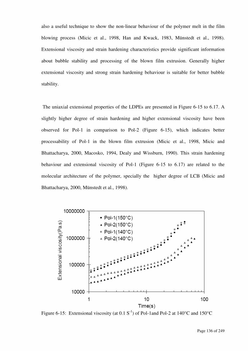
Page 136 of 249
also a useful technique to show the non-linear behaviour of the polymer melt in the film
blowing process (Micic et al., 1998, Han and Kwack, 1983, Münstedt et al., 1998).
Extensional viscosity and strain hardening characteristics provide significant information
about bubble stability and processing of the blown film extrusion. Generally higher
extensional viscosity and strong strain hardening behaviour is suitable for better bubble
stability.
The uniaxial extensional properties of the LDPEs are presented in Figure 6-15 to 6.17. A
slightly higher degree of strain hardening and higher extensional viscosity have been
observed for Pol-1 in comparison to Pol-2 (Figure 6-15), which indicates better
processability of Pol-1 in the blown film extrusion (Micic et al., 1998, Micic and
Bhattacharya, 2000, Macosko, 1994, Dealy and Wissburn, 1990). This strain hardening
behaviour and extensional viscosity of Pol-1 (Figure 6-15 to 6.17) are related to the
molecular architecture of the polymer, specially the higher degree of LCB (Micic and
Bhattacharya, 2000, Münstedt et al., 1998).
Figure 6-15: Extensional viscosity (at 0.1 S
-1) of Pol-1and Pol-2 at 140°C and 150°C

Page 137 of 249
Strain hardening parameter (SHP) can be quantified using the ratio of the extensional
viscosity in the strain hardening region and that in the linear region of the same run (Micic
et al., 1998). In this study, SHP of Pol-1 and Pol-2 was determined at three different
temperatures (Table 6-6) using the extensional viscosity in three different strain hardening
zones (at 20s, 35s and 40s) and that in linear zone (at 5s). The values of SHP presented in
Table 6-6, show an expected decrease in strain hardening characteristics for both resins
with increasing temperatures.
Table 6-6 : Strain hardening parameter of the LDPEs at different temperatures and
different using different extensional viscosity
Strain Hardening Parameter(SHP) using the viscosity at 5sec and
20sec 35sec 40sec
Temperature(°C) Pol-1 Pol-2 Pol-1 Pol-2 Pol-1 Pol-2
140 3.6 2.2 12.6 5.4 16.9 7.2
150 3.5 2.1 11.6 4.4 15.9 5.8
170 3.3 2.0 11.4 3.1 15.5 3.8
At the experimental temperatures (140°C, 150°C and 170°C), Pol-1 molecules may have
had more entanglement (due to higher Mw and higher degree of LCB) (Figure 6-16) during
uniaxial extension in the RME rheometer in comparison to Pol-2 (Figure 6-17). Therefore,
the effect of experimental temperature on melt extensibility is relatively less obvious for
Pol-1 (Figure 6-16) because of its higher value of Mw and LCB, whereas it is significant
for Pol-2 (Figure 6-17). Due to the lower value of flow activation energy (52.01 kJ/mol),
slippage properties of Pol-2 molecules are higher and hence uniaxial extensional viscosity
of Pol-2 is relatively lower than Pol-1. Therefore, molecular structures are playing an
important role for the temperature dependency on the extensional rheology of the LDPEs.
Higher degree of LCB in Pol-1 shows the greatest degree of extensional thickening (strain
hardening) during the free surface flows along with the effect of stress induced
crystallization, which has substantial implications for processing. Hence, it can be said that
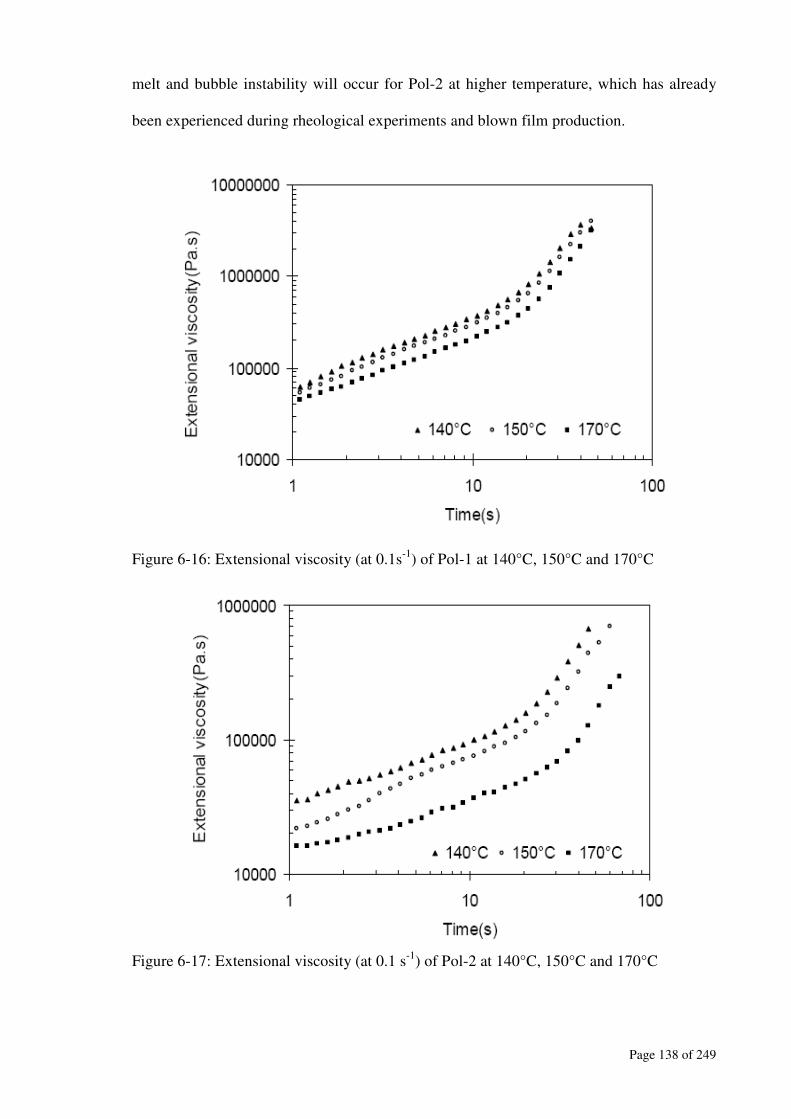
Page 138 of 249
melt and bubble instability will occur for Pol-2 at higher temperature, which has already
been experienced during rheological experiments and blown film production.
Figure 6-16: Extensional viscosity (at 0.1s-1
) of Pol-1 at 140°C, 150°C and 170°C
Figure 6-17: Extensional viscosity (at 0.1 s
-1) of Pol-2 at 140°C, 150°C and 170°C

Page 139 of 249
In the RME rheometer, total Hencky strain attained was 7, which is related well with the
Hencky strain (about 3.7 for a draw ratio of 40) that is usually observed during blown film
extrusion (Micic et al., 1998). Hence, the deformation achieved in the extensional
experiments and presented here is a snapshot of the deformation in the real film blowing
process. It is also essential to describe the importance of the linear and strain hardening
zone to relate with the blown film processability. In this study, a critical Hencky strain of
about 2.0 is observed for a transition from the linear zone to the strain hardening zone for
both Pol-1 and Pol-2. Therefore, strain hardening zone (Hencky strain>2.0) is more
important (or significant) than the linear zone to determine the blown film processability of
the LDPEs. Helical and frost line instability of the bubble was observed for Pol-2 at 220°C
in the pilot plant, whereas Pol-1 was found stable at that temperature. Therefore, it can be
argued that lower values of SHP of Pol-2 (Table 6-6) are related to its blown film
processability at higher temperatures (220°C and above).
6.4 Thermal analysis
Like rheological study, structural variations of the polymers can be observed by their
thermal analysis either from heating or cooling cycle or combination of both. Modulated
differential scanning calorimetry (MDSC) was used for thermal analysis of the LDPEs.
Thermal properties of Pol-1 and Pol-2 were determined using two different types of
samples (pellet and plaque) (Figure 6-18) before processing and a blown film sample
obtained at different cooling rates (Figures 6-19 to 6-21). Freeze line height (FLH) which
varies with the cooling rates and molecular structure of the LDPE is related with blown
film crystallinity. This FLH is an important parameter to analyse the blown film optical,
shrinkage and tear properties. Therefore, blown films of Pol-1 and Pol-2 processed at
different cooling rates were also considered for the thermal study (Figures 6-20 and 6-21)
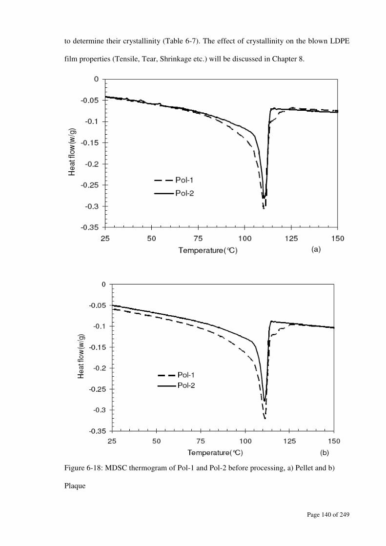
Page 140 of 249
to determine their crystallinity (Table 6-7). The effect of crystallinity on the blown LDPE
film properties (Tensile, Tear, Shrinkage etc.) will be discussed in Chapter 8.
Figure 6-18: MDSC thermogram of Pol-1 and Pol-2 before processing, a) Pellet and b)
Plaque
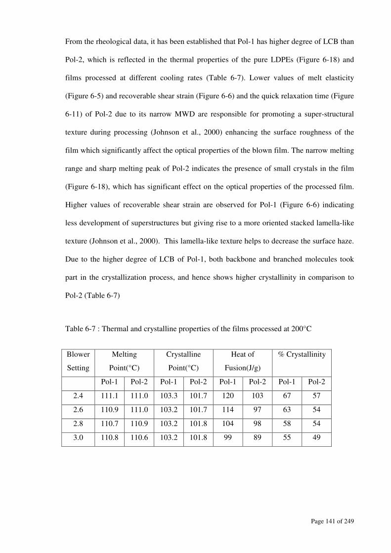
Page 141 of 249
From the rheological data, it has been established that Pol-1 has higher degree of LCB than
Pol-2, which is reflected in the thermal properties of the pure LDPEs (Figure 6-18) and
films processed at different cooling rates (Table 6-7). Lower values of melt elasticity
(Figure 6-5) and recoverable shear strain (Figure 6-6) and the quick relaxation time (Figure
6-11) of Pol-2 due to its narrow MWD are responsible for promoting a super-structural
texture during processing (Johnson et al., 2000) enhancing the surface roughness of the
film which significantly affect the optical properties of the blown film. The narrow melting
range and sharp melting peak of Pol-2 indicates the presence of small crystals in the film
(Figure 6-18), which has significant effect on the optical properties of the processed film.
Higher values of recoverable shear strain are observed for Pol-1 (Figure 6-6) indicating
less development of superstructures but giving rise to a more oriented stacked lamella-like
texture (Johnson et al., 2000). This lamella-like texture helps to decrease the surface haze.
Due to the higher degree of LCB of Pol-1, both backbone and branched molecules took
part in the crystallization process, and hence shows higher crystallinity in comparison to
Pol-2 (Table 6-7)
Table 6-7 : Thermal and crystalline properties of the films processed at 200°C
Blower
Setting
Melting
Point(°C)
Crystalline
Point(°C)
Heat of
Fusion(J/g)
% Crystallinity
Pol-1 Pol-2 Pol-1 Pol-2 Pol-1 Pol-2 Pol-1 Pol-2
2.4 111.1 111.0 103.3 101.7 120 103 67 57
2.6 110.9 111.0 103.2 101.7 114 97 63 54
2.8 110.7 110.9 103.2 101.8 104 98 58 54
3.0 110.8 110.6 103.2 101.8 99 89 55 49
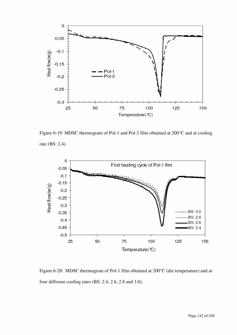
Page 142 of 249
Figure 6-19: MDSC thermogram of Pol-1 and Pol-2 film obtained at 200°C and at cooling
rate (BS: 2.4).
Figure 6-20: MDSC thermogram of Pol-1 film obtained at 200°C (die temperature) and at
four different cooling rates (BS: 2.4, 2.6, 2.8 and 3.0).
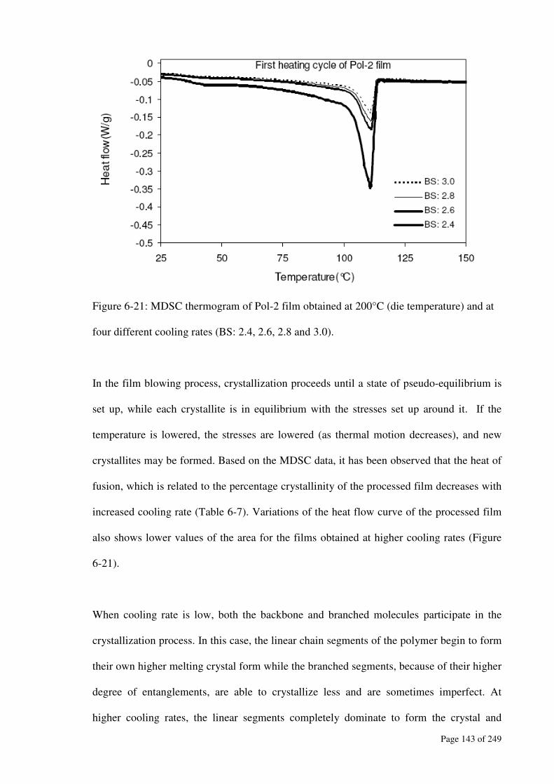
Page 143 of 249
Figure 6-21: MDSC thermogram of Pol-2 film obtained at 200°C (die temperature) and at
four different cooling rates (BS: 2.4, 2.6, 2.8 and 3.0).
In the film blowing process, crystallization proceeds until a state of pseudo-equilibrium is
set up, while each crystallite is in equilibrium with the stresses set up around it. If the
temperature is lowered, the stresses are lowered (as thermal motion decreases), and new
crystallites may be formed. Based on the MDSC data, it has been observed that the heat of
fusion, which is related to the percentage crystallinity of the processed film decreases with
increased cooling rate (Table 6-7). Variations of the heat flow curve of the processed film
also shows lower values of the area for the films obtained at higher cooling rates (Figure
6-21).
When cooling rate is low, both the backbone and branched molecules participate in the
crystallization process. In this case, the linear chain segments of the polymer begin to form
their own higher melting crystal form while the branched segments, because of their higher
degree of entanglements, are able to crystallize less and are sometimes imperfect. At
higher cooling rates, the linear segments completely dominate to form the crystal and

Page 144 of 249
contributions of branched segments are much less, or zero, depending on the branching
characteristics of the resin. If the bubble is cooled very slowly the specific volume will
reach a lower value than at a relatively high cooling rate. At a low cooling rate the polymer
chains, because of their thermal motion, have more opportunity to position them closer
together and enhances the order of the molecules. This reduces the free volume of the
polymers.
6.5 WAXD analysis
In the WAXD experiment, an X-Ray of a given wavelength impinges on the crystal
structure and diffracted into a large number of narrow beams imperceptible by the
photographic film or by Geiger counter. The angle of scattering depends on the order of the
chains within the polymer. WAXD study of the semicrystalline polymers shows wider
peaks on a raised background that shows the interatomic distance of the less ordered
crystalline planes (Halasa et al., 1991) and sharp peaks in the WAXD plot indicate the
presence of smaller sizes of spherulite (Majumder et al., 2007a).
WAXD data of the LDPEs (Pol-1 and Pol-2 in plaque form) were obtained using a
rotational sample holder during experimentation. From this analysis, it has been observed
that Pol-1 and Pol-2 show almost identical crystalline properties (Figure 6-22) before
processing in the blown film line, whereas their thermal properties showed a significant
difference (Figure 6-18). Primary differences between the LDPEs are the molecular
structure (Table 6-1) and the degree of orientation (i.e., the orientation of the lamellar
structures) on a nanoscale (Bafna et al., 2001). Therefore, it can be said that WAXD study
couldn’t differentiate the molecular architecture of the LDPEs when they remain as a solid
plaque.
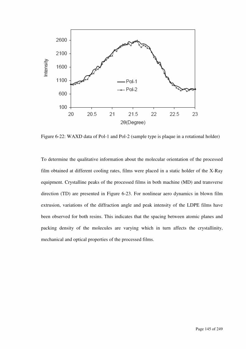
Page 145 of 249
Figure 6-22: WAXD data of Pol-1 and Pol-2 (sample type is plaque in a rotational holder)
To determine the qualitative information about the molecular orientation of the processed
film obtained at different cooling rates, films were placed in a static holder of the X-Ray
equipment. Crystalline peaks of the processed films in both machine (MD) and transverse
direction (TD) are presented in Figure 6-23. For nonlinear aero dynamics in blown film
extrusion, variations of the diffraction angle and peak intensity of the LDPE films have
been observed for both resins. This indicates that the spacing between atomic planes and
packing density of the molecules are varying which in turn affects the crystallinity,
mechanical and optical properties of the processed films.
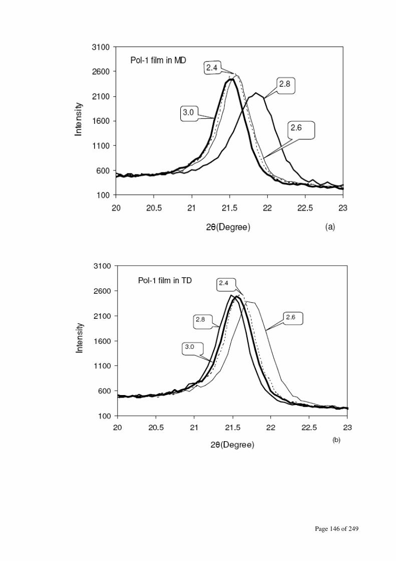
Page 146 of 249

Page 147 of 249
Figure 6-23: WAXD plot of Pol-1((a) and (b)) and Pol-2((c) and (d)) films processed at
200°C (die temperature) and different blower settings (2.4, 2.6, 2.8 and 3.0).

Page 148 of 249
Molecular orientations in the processed blown films are the result of biaxial deformation,
which is significantly influenced by the cooling rates (while other process variables remain
constant). Semicrystalline polymers like LDPE have different degrees of orientation, based
on their crystalline and amorphous components. X-Ray techniques are useful to determine
this morphology and have been found to vary depending on the nature (size or packing
pattern) of the crystal lattice (Gordon, 1963). Like the heat flow curve, WAXD peak and
width are used to determine the percent crystallinity. However, only WAXD width has
been considered here to get an idea about the molecular orientations of the processed films
(Figure 6-23). A variation of the WAXD plots have been observed for the processed films
obtained at different cooling rates, due to the configuration of the individual chains and
their mode of packing during biaxial stretching. MDSC experiments revealed that
percentage crystallinity increases with the cooling rates for both LDPEs. From the WAXD
study, it has also been found that relatively wider peaks occur at higher cooling rates
(Figure 6-23), which indicates less ordered crystalline planes (Halasa et al., 1991).
Therefore, it can be argued that qualitative information of WAXD results agreed well with
the quantitative information of MDSC study.
6.6 Summary
Pol-1 shows higher zero shear viscosity and relaxation time than Pol-2 due to its higher
molecular weight and long chain branching (LCB) characteristics. LCB plays an important
role in melt elasticity and amorphous orientation (tie molecules between lamellae) during
blown film processing, which ultimately affect film crystallinity, mechanical and thermal
properties. Lower value of melt elasticity, which is related to short relaxation time,
promotes more spherulitic-like superstructural element in the film. Higher shear thinning
properties of Pol-1 were due to the broad MWD, more branching and higher degree of LCB.
Page 149 of 249
From the extensional rheological experiments, it is observed that Pol-1 shows higher
extensional viscosity and strain hardening in comparison to Pol-2 due to the higher values of
molecular weight and higher degree of LCB. These higher extensional properties of Pol-1
will support for blown film bubble stability.
Sharp crystalline peaks and narrow crystal size distribution of Pol-2 were obtained in both
WAXD and MDSC studies due to the absence of high molecular weight chain. For Pol-1,
long branched molecules along with the main chain participated in the crystallization
process, producing more crystallinity than Pol-2. Nonlinear relationship of the film strength
with the cooling rates in blown film process properties have been obtained due to the non-
isothermal melt flow and melt elasticity, which affect the spacing between the molecules in
the films as observed in WAXD analysis.

Page 150 of 249
CHAPTER : 7
Establishment of a Rheological Constitutive Equation and Results of Blown Film Simulation
The developments and limitations of the previous rheological models used in the
simulation of blown film process are already presented in Chapter 3. Following those
limitations reported, in the earlier part of this chapter, discussion will be presented on the
development of a new rheological constitutive equation for use in the blown film
modelling. The numerical results of the blown film simulation will be presented here for
both LDPEs. The choice of the rheological constitutive equation will also be justified by
comparing the results of other viscoelastic models. Numerical predictions of the blown
film process characteristics will be verified using the data from the pilot plant study
(Majumder et al., 2007b) and a set of data obtained from the work of Muke et al (2003).
7.1 Governing equations
The governing equations of the film blowing process are derived on the basis of similar
assumptions as discussed in Chapter 3 (First paragraph of Section 3.2). The flow chart of
blown film equations and computational techniques are presented in Figure 7-1.

Page 151 of 249
Figure 7-1: Development of the Blown film model and computational technique.
7.1.1 Fundamental film blowing equations
Considering the thin film bubble membrane by Pearson and Petrie (1970), the bubble is
assumed to have two radii of curvature R1 (in the machine direction) and R3 (in the
transverse or hoop direction), which can be expressed in terms of the following
expressions:
22
2/32
22
3
1/
])/(1[
/
sec
dzrd
dzdr
dzrdR
+−=
−=
θ (7-1)
2
3 )/(1cos
dzdrrr
R +==θ
(7-2)
dz
dr=θtan (7-3)
According to the conservation of mass, the mass flow rate,
rHVvrrmsmi
πρρπ 2)( 0
22
0
.
=−= (7-4)
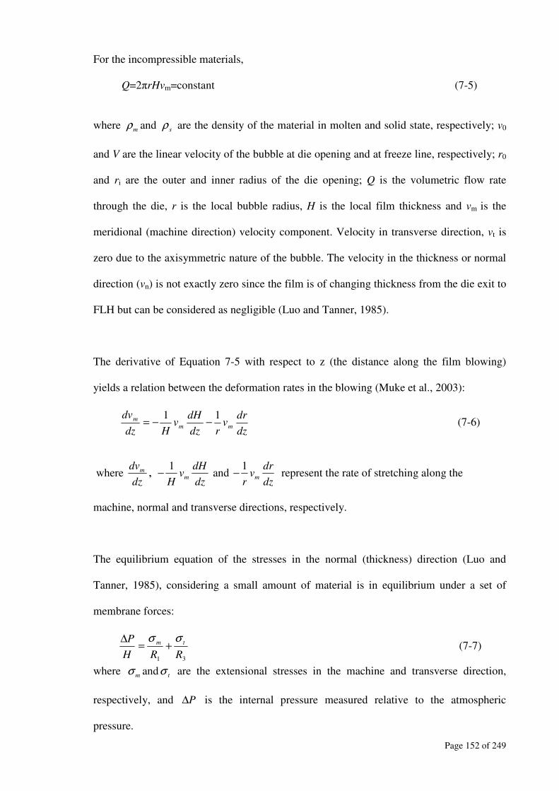
Page 152 of 249
For the incompressible materials,
Q=2πrHvm=constant (7-5)
where m
ρ and s
ρ are the density of the material in molten and solid state, respectively; v0
and V are the linear velocity of the bubble at die opening and at freeze line, respectively; r0
and ri are the outer and inner radius of the die opening; Q is the volumetric flow rate
through the die, r is the local bubble radius, H is the local film thickness and vm is the
meridional (machine direction) velocity component. Velocity in transverse direction, vt is
zero due to the axisymmetric nature of the bubble. The velocity in the thickness or normal
direction (vn) is not exactly zero since the film is of changing thickness from the die exit to
FLH but can be considered as negligible (Luo and Tanner, 1985).
The derivative of Equation 7-5 with respect to z (the distance along the film blowing)
yields a relation between the deformation rates in the blowing (Muke et al., 2003):
dz
drv
rdz
dHv
Hdz
dv
mm
m11
−−= (7-6)
where dz
dvm
, dz
dHv
Hm
1− and
dz
drv
rm
1− represent the rate of stretching along the
machine, normal and transverse directions, respectively.
The equilibrium equation of the stresses in the normal (thickness) direction (Luo and
Tanner, 1985), considering a small amount of material is in equilibrium under a set of
membrane forces:
31 RRH
Ptm
σσ+=
∆ (7-7)
where m
σ andt
σ are the extensional stresses in the machine and transverse direction,
respectively, and P∆ is the internal pressure measured relative to the atmospheric
pressure.

Page 153 of 249
Replacing R1 and R3 in Equation 7-7 yields:
−=
∆
dz
d
rH
P
m
tθ
σσ
θcos (7-8)
According to previous studies (Gupta and Metzner, 1982, Gupta et al., 1982, Muke et al.,
2003), the total force F, balanced by F (z), Fg (z) and Fp (z) (see Figure 2-1 in Chapter 2 ),
is shown in the following equation:
F = F (z) + Fg (z) - Fp (z) (7-9)
where F (z) is the axial component of the forces generated due to the deformation of the
material; Fp (z) is the force due to the pressure difference between inside and outside of the
bubble; and Fg (z) is the force due to gravity. In this study, the gravity force Fg (z) has
been neglected. Hence,
F (z) = Fp (z) +F (7-10)
θσππ cos2)()(2
0
2
mHrrrpzF +−∆−= (7-11)
where 2
2/12
'1
11cos
rdz
dr
+=
+=
−
θ
Differentiating Equation 7-11 and rearranging it with Equation 7-8 yields,
−−=
H
H
r
r
m
t
mm
')1(
''
σ
σσσ (7-12)
Rearranging and combining Equations 7-1 to 7-12, gives the dimensionless fundamental
film blowing equations irrespective of the rheological constitutive equations (Muke et al.,
2003):
L=rh
rBrA22 '1)( ++
(7-13)
2
22" )]'1(2'1[
BrA
rrBrhCr
+
+−+= (7-14)
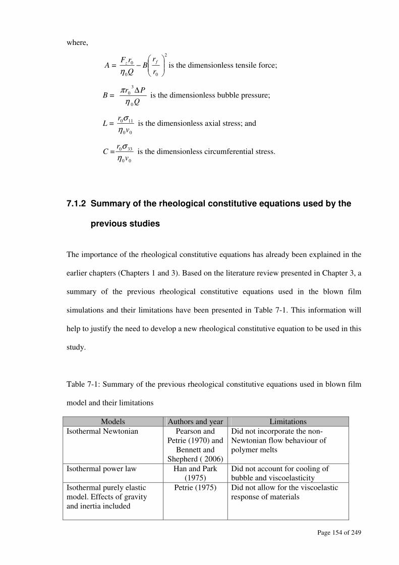
Page 154 of 249
where,
A =
2
00
0
−
r
rB
Q
rF fz
ηis the dimensionless tensile force;
B = Q
Pr
0
3
0
η
π ∆ is the dimensionless bubble pressure;
L = 00
110
v
r
η
σ is the dimensionless axial stress; and
C =00
330
v
r
η
σ is the dimensionless circumferential stress.
7.1.2 Summary of the rheological constitutive equations used by the
previous studies
The importance of the rheological constitutive equations has already been explained in the
earlier chapters (Chapters 1 and 3). Based on the literature review presented in Chapter 3, a
summary of the previous rheological constitutive equations used in the blown film
simulations and their limitations have been presented in Table 7-1. This information will
help to justify the need to develop a new rheological constitutive equation to be used in this
study.
Table 7-1: Summary of the previous rheological constitutive equations used in blown film
model and their limitations
Models Authors and year Limitations
Isothermal Newtonian
Pearson and
Petrie (1970) and
Bennett and
Shepherd ( 2006)
Did not incorporate the non-
Newtonian flow behaviour of
polymer melts
Isothermal power law Han and Park
(1975)
Did not account for cooling of
bubble and viscoelasticity
Isothermal purely elastic
model. Effects of gravity
and inertia included
Petrie (1975) Did not allow for the viscoelastic
response of materials
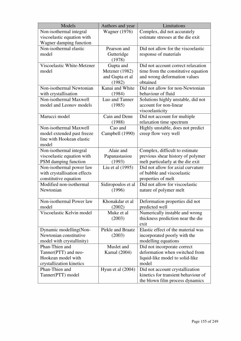
Page 155 of 249
Models Authors and year Limitations
Non-isothermal integral
viscoelastic equation with
Wagner damping function
Wagner (1976) Complex, did not accurately
estimate stresses at the die exit
Non-isothermal elastic
model
Pearson and
Gutteridge
(1978)
Did not allow for the viscoelastic
response of materials
Viscoelastic White-Metzner
model
Gupta and
Metzner (1982)
and Gupta et al
(1982)
Did not account correct relaxation
time from the constitutive equation
and wrong deformation values
obtained
Non-isothermal Newtonian
with crystallisation
Kanai and White
(1984)
Did not allow for non-Newtonian
behaviour of fluid
Non-isothermal Maxwell
model and Leonov models
Luo and Tanner
(1985)
Solutions highly unstable, did not
account for non-linear
viscoelasticity
Marucci model Cain and Denn
(1988)
Did not account for multiple
relaxation time spectrum
Non-isothermal Maxwell
model extended past freeze
line with Hookean elastic
model
Cao and
Campbell (1990)
Highly unstable, does not predict
creep flow very well
Non-isothermal integral
viscoelastic equation with
PSM damping function
Alaie and
Papanastasiou
(1993)
Complex, difficult to estimate
previous shear history of polymer
melt particularly at the die exit
Non-isothermal power law
with crystallisation effects
constitutive equation
Liu et al (1995) Did not allow for axial curvature
of bubble and viscoelastic
properties of melt
Modified non-isothermal
Newtonian
Sidiropoulos et al
(1996)
Did not allow for viscoelastic
nature of polymer melt
Non-isothermal Power law
model
Khonakdar et al
(2002)
Deformation properties did not
predicted well
Viscoelastic Kelvin model Muke et al
(2003)
Numerically instable and wrong
thickness prediction near the die
exit
Dynamic modelling(Non-
Newtonian constitutive
model with crystallinity)
Pirkle and Braatz
(2003)
Elastic effect of the material was
incorporated poorly with the
modelling equations
Phan-Thien and
Tanner(PTT) and neo-
Hookean model with
crystallization kinetics
Muslet and
Kamal (2004)
Did not incorporate correct
deformation when switched from
liquid-like model to solid-like
model
Phan-Thien and
Tanner(PTT) model
Hyun et al (2004) Did not account crystallization
kinetics for transient behaviour of
the blown film process dynamics
Page 156 of 249
7.1.3 Rheological constitutive equations developed in this study
Based on the discussion in Chapter 3 and Table 7-1, it has been revealed that PTT model
provides better rheological properties in the melt state. In the film blowing process, this
model is mostly suitable for incorporating the material properties near the die exit. Since,
polymer melt is transformed to a solid phase due to crystallization near the freeze line
height, another rheological/crystallization model is required to incorporate solid state
properties of the polymer. Cao and Campbell (1990) used two different rheological models
in their blown film simulation. They used the Maxwell model to incorporate viscoelastic
properties of the melt and the Hookean model for elastic/solid properties. However,
Maxwell model provides reasonable viscoelastic properties at small deformation rates only
and its numerical solution is complex (Luo and Tanner, 1985, Muke et al., 2003). To
incorporate solid state properties of the material, Muslet and Kamal (2004) used neo-
Hookean and crystallization models. They used various numerical techniques to solve the
blown film equations. In their simulation, bubble characteristics (bubble size and film
thickness) were predicted inconsistently with respect to materials deformation while
transiting from liquid to the solid state and prediction shows several limitations in practice.
In order to achieve simplicity, numerical stability, faster and reasonable performance to
simulate a film blowing process, a new rheological constitutive equation is proposed by
combining the well known PTT model and the Hookean model as shown in Equation 7-15.
Addition of an elastic model with the PTT model will provide better elastic properties of
the melt near the freezing line and will provide a quick numerical solution with very less
numerical instability in comparison to previous studies. It is also expected that this model
will achieve a reasonable prediction from the blown film simulation for FLH and bubble
characteristics (bubble diameter, film thickness and film temperature), useful to the film
blowing industry. This will also allow a quick check of film properties as they are linked

Page 157 of 249
with FLH and bubble characteristics. This simulation will save a lot of material, labour and
time required for doing trial runs.
In this study, the total stress (τ) is considered as
τ = Melt state, τm (PTT model) + Solid state τs (Hookean model) (7-15)
According to the previous studies (Muslet and Kamal, 2004, Hyun et al., 2004) , PTT
model for the molten state is expressed as,
i
εη ɺ2 = τi Y (τ) + λ [∇
iτ + 2ξ (τi
iεɺ )] (7-16)
Therefore,
Total stress, τi = τi Y (τ) + λ [∇
iτ +2ξ (τi
iεɺ )] + 2G0
iε (7-17)
where,
∇
iτ = t
ii
dt
d]][[]][[ νττν
τ∇−∇− ,
Y (τ) = exp (i
trτη
ελ),
iεɺ is deformation rate tensor,
i
ε is deformation tensor,
0G is elastic modulus
ε is extensional property of the film in the PTT model (Muslet and Kamal, 2004),
ξ is Slippage parameter of the polymer chains in the PTT model (Muslet and Kamal,
2004)
The rates of deformation tensor in the surface coordinate system can be expressed in terms
of the film velocity (v), bubble radius (r), film thickness (h), angle of film blowing (θ) and
the distance from the die (z):

Page 158 of 249
7.1.4 Development of the blown film equations
The force balance equations (Equations 7-13 and 7-14) and rheological constitutive
equation (Equation 7-17) are coupled together to relate the stresses to the strains or strain
rates in a bubble, in order to predict the various film blowing process characteristics .
The rates of deformation acting on an element of fluid in the three principal directions are
given as (Muke et al., 2003) :
)''
('1 2
11
.
r
r
H
H
r
v−−
+=ε (7-19)
222
.
'1
'
rH
vH
+=ε (7-20)
2
.
33
'
'
rrr
vr
+=ε (7-21)
In the above equations and hereafter, prime refers to the derivatives with respect to the
distance from the die exit. Hence, the deviatoric stresses in the three principal directions
are:
( )
−
−+−= 11011
.
11
11 2)1(21cos
1εελξττ
θλ
τGY
vdz
d (7-22)
( )
−
−+−= 22022
.
22
22 2)1(21cos
1εελξττ
θλ
τGY
vdz
d (7-23)
( )
−
−+−= 33033
.
33
33 2)1(21cos
1εελξττ
θλ
τGY
vdz
d (7-24)
dz
dv
v
1 0 0
iεɺ = vcosθ 0
dz
dh
h
1 0
0 0 dz
dr
r
1
(7-18)

Page 159 of 249
The total stress for each of the component is related to the deviatoric stresses (Muke et al.,
2003) by:
ijijijpδτσ −= (7-25)
where p is the isotropic pressure, ij
τ is the deviatoric stress and ij
δ is the Kronecker delta:
≠
==
ji
ji
ij
0
1δ . The stress at the free surface is equal to atmospheric pressure (Muke et
al., 2003) .This gives: p= 22τ and hence
221111 ττσ −= (7-26)
223333 ττσ −= (7-27)
By introducing the following dimensionless terms into the above equations (Equations 7-
25 to 7-27):
0H
Hh = ,
0r
Rr = ,
0r
Zz = ,
0v
Vv = ,
a
a
T
TTt
−= , De=
00
00
0
0
rG
v
r
v ηλ= ,
0
)(
η
ηη
T= ,
00
110
η
σ
v
rL = and
00
330
η
σ
v
rC =
and rearranging these equations to obtain the differential stresses with respect to z in the
machine, transverse and normal(thickness) directions , respectively:
[ ]
2
2
2
2
1ln2
''2
'1)1(2
''
'1)1(2)(1'
De
rh
r
r
h
h
r
Pv
r
r
h
h
r
LvY
De
LL
−
+
+−
−
+
+−−−=
ξ
ξτ
(7-28)
[ ]
22
2
ln2''
'1)1(2
'1
')1(2)(1'
De
h
r
r
r
h
h
r
Pv
rr
CvrY
De
CC
−
+
+−
+
+−+−=
ξ
ξτ
(7-29)

Page 160 of 249
( )2222
'1
')1(2)ln(2)(1'
rh
Pvh
De
hY
De
P
+
−+−−=
ξττ (7-30)
where, Y (τ) = exp ( )
++ 332211 τττ
η
εDe
Equations 7-13, 7-14 and 7-28 to 7-30 are combined to obtain the following non-linear
differential equation to determine bubble characteristics:
( )
+
+
+
−
+−−
−=
+
+−−
22
112
11
33
112
1ln
21
'1
')1(2
)(11
1'2
1'1
)1(21'
rhDe
P
rr
vr
YDer
rP
r
v
h
h
σ
ξ
τσ
σ
σξ
(7-31)
Though a complex thermodynamics is involved during film blown process due to the effect
of cooling air and other process dynamics, most blown film modelling (Cao and Campbell,
1990, Muke et al., 2003, Kanai and White, 1984, Luo and Tanner, 1985) ignored the
dynamic effect and treated it as a constant heat transfer coefficient. In this study, the
thermodynamic effect is considered by incorporating a modified heat transfer function
(Equation 7-32) from the previous studies (Muslet and Kamal, 2004, Sidiropoulos, 2000)
with the dimensionless energy equation (Luo and Tanner, 1985). End effect of the cooling
air at the lip of the die exit and after the freeze line was not counted in Equation 7-83. It
incorporates the effect of the temperature difference between the film surfaces, velocity of
the cooling air and radius of the bubble on the heat transfer coefficient, Hc:
( )( )[ ]( )z
rTTVH
airsurfaceair
c
exp1
035.027.1exp780560084.0
+
−−−−= (7-32)
The dimensionless energy equation (Luo and Tanner, 1985) used in this study is
2'1'''
' rrtCr
r
h
hL
r
rCCt
he+−
+−= (7-33)
Page 161 of 249
where,
ap
e
TCha
QC
ρπ
η
0
2
0
0
2= is the dimensionless energy dissipation coefficient and
QC
HaC
p
c
h
ρ
π 2
02= is the dimensionless heat transfer coefficient
According to the previous studies (Muke et al., 2003, Luo and Tanner, 1985), the
following temperature dependence of viscosity function (Arrhenius type) is used here:
−=
0
000
11)()(
TTEaExpTT ηη (7-34)
7.2 Numerical techniques
Dynamic or transient solutions are usually more accurate for any dynamic process like
blown film extrusion. However, these techniques involve a lot of numerical complexity to
consider all dynamic instabilities during processing. Steady state solutions are simple,
quick and provide reasonable predictions for engineering needs. Therefore, this study is
focussed to steady state solution of the blown film process to obtain the freeze line height
and bubble characteristics with a reasonable accuracy.
A fourth-order Runge-Kutta method (Kutta-Simpson 1/3 rule) is used to solve the
differential equations (Equations 7-28 to 7-31 and Equation 7-33). It requires four
evaluations per step and provides an excellent balance of power, precision and simple to
code in any numerical solver. Several researchers (Muke et al., 2003, Muslet and Kamal,
2004, Luo and Tanner, 1985) used this technique to solve the blown film equations.
A step size of 0.01 has been used to solve the film blowing equations (Equations 7-28 to 7-
31 and Equation 7-33) simultaneously. Following the Runge-Kutta fourth order Kutta-
Simpson 1/3 rule, programming codes have been written in Maple-10 for numerical

Page 162 of 249
integration of those equations (Appendix A4). All calculations started with the parameters
at the die exit (Table 7-2) and continued until the changes in the bubble expansion and
thickness reduction with respect to the dimensionless axial distance become negligible or
zero( 0≈dz
dr and 0≈
dz
dh). The axial distance in the direction of flow where 0≈
dz
dr and
0≈dz
dh is considered as the freeze line height (FLH).
7.2.1 Boundary conditions
The following boundary conditions were used in the modelling equations-
At die exit (z = 0), r =1 (bubble diameter is equal to the die diameter),
h =1(bubble thickness is equal to the die gap) and
a
adie
T
TTt
−= (
dieT is the temperature at the die exit)
At freeze line position (z= ZFL), 0=dz
dr(bubble expansion is zero or negligible with
respect to the dimensionless axial distance).
7.2.2 Materials and process parameters at the die exit
Two different die temperatures have been used for blown film simulation; (i) 200°C by
Majumder et al (2007b), and (ii) 210°C by Muke et al (2003). The rheological properties of
Pol-1 and Pol-2 have already been discussed in Chapter 5 and used in the blown film
simulation. For Polypropylene homopolymer, rheological, process and experimental data
were obtained from the literature (Muke et al., 2003). The initial values of the material
properties at die temperatures and process parameters are presented in Table 7-2.

Page 163 of 249
Table 7-2: Rheological and processing parameters of the resins used in the modelling
Inputs Pol-1 Pol-2 Polypropylene
homopolymer,
MA-3 (Muke et
al., 2003)
Density(kg/m3), ρ 922 922 900
Zero shear viscosity( Pa.s), η0 96503
(at 200°C)
26000
(at 200°C)
22800
(at 210°C)
Relaxation time(s),λ 14.65
(at 200°C)
1.74
(at 200°C)
18.4
(at 210°C
Flow activation energy(°K),Ea 6845 6255 4924
Mass flow rate (kg/hr) , .
m 7.5 7.5 3.9
Ambient temperature(°C),Ta 25 25 25
Die temperature(°C),T0 200 200 210
Die diameter(mm),d0 65 65 40
Die gap(mm),H0 2.038 2.038 0.75
Crystallization temperature(°C) 103 103 123
Deborah number(λv0/r0), De 6.8 0.696 7.11
Extensional property, ε 0.15 0.15 0.15
Slippage property of the chain, ξ 0.147 0.147 0.147
Velocity at die(m/s),v0 0.013 0.013 0.0077
Dimensionless tensile force, A 0.61 0.61 0.83885
Dimensionless bubble pressure ,B 0.2035 0.2035 0.38773
Dimensionless energy dissipation
coefficient, Ce
0.000034402 0.00000932 0.00002234
7.3 Results and discussion
Prediction of the freezing line height (FLH) and bubble characteristics (diameter, thickness
and temperature) at FLH are the most useful information for the flexible film packaging
industry. Therefore, it is necessary to discuss about the modelling outputs first, i.e. whether
they are showing a realistic prediction before comparing them with the experimental data.
According to the previous studies (Muslet and Kamal, 2004, Hyun et al., 2004), PTT
model is best suitable to describe stress and deformation properties of a polymer when it
is in the molten state and in the field of extension. Therefore, the prediction might not be
correct close to the freezing line if only the PTT model is used. It is argued that a solid-like
rheological model (such as Hookean model) may make a better prediction close to the
FLH, since the material changes from liquid to solid state close to the freezing line.
Page 164 of 249
Furthermore, a significant region between the die exit and the FLH deals with liquid- solid
transition since heat transfer occurs arising from the cooling effect. There is no rheological
model available in the literature to describe the stress and deformation properties in this
transition. Several researchers (Luo and Tanner, 1985, Cao and Campbell, 1990, Ghaneh-
Fard et al., 1996, Gupta et al., 1982, Han and Park, 1975a, Hyun et al., 2004, Kanai and
White, 1984, Khonakdar et al., 2002, Muslet and Kamal, 2004, Muke et al., 2003)
presented their works without properly justifying this effect. Hence, one of the main
objectives of this work is to model the stress and deformation properties in that critical
zone (liquid-solid transition) using a rheological constitutive equation combining both the
PTT and the Hookean model (Equation 7-17). Muslet and Kamal (2004) published an
extensive study considering film crystallinity and viscoelasticity of the material. However,
their model predictions showed significant deformation of the film in all (machine,
transverse and thickness) directions even after the freeze line height. This is impractical in
the blown film process and also contradictory to their result of the bubble diameter which
was predicted constant after the freezing line. Their result also showed a sharp transition in
the curve that was used to predict the film thickness when the model input parameters
shifted from liquid to sold state. That is why the profiles of the film thickness, stress and
deformation weren’t smooth in their prediction due to the use of inaccurate rheological
properties. Those issues have been solved in the present work by incorporating the
proposed constitutive equation (Equation 7-17) into the fundamental film equations
(Equations 7-13 and 7-14).
7.3.1 Prediction of bubble characteristics
Instead of focussing on the blowing angle near the die as was done by several researchers
(Luo and Tanner, 1985, Muslet and Kamal, 2004, Cao and Campbell, 1990) or any
calculations after the FLH (Cao and Campbell, 1990, Muslet and Kamal, 2004), the present
study focussed on the prediction of freeze line height (FLH) and bubble characteristics at

Page 165 of 249
that FLH. The effect of Deborah No ( 000 / rvDe λ= ) on the bubble shape is compared by
Muslet and Kamal (2004) with the prediction of Luo and Tanner (1985). The results of the
bubble diameter predicted by the present model are shown in Figure 7-2. Similar to earlier
study, it can be seen that the bubble diameter decreases as the Deborah No (De0) increases
for both materials (Pol-1 and Pol-2).
Figure 7-2: Effect of Deborah number (De0=
0
0
r
vλ) on the bubble shape as – (a) Pol-1, (b)
Pol-2

Page 166 of 249
7.3.1.1 Heat transfer coefficient
A realistic value of heat transfer coefficient is required to simulate an actual film process
due to its rapid changes of temperature from die exit to the freeze line height and above.
Several studies (Cao and Campbell, 1990, Liu et al., 1995, Luo and Tanner, 1985) in the
literature simulated the blown film process using a constant value (10 to 20 w.k-1
.m-2
) of
heat transfer coefficient. But in real practice, the rate of heat transfer is higher than those
values at the die exit and then decreases along the direction of flow. In this study, a heat
transfer function (Equation 7-32) has been used with the energy equation (Equation 7-33)
to incorporate a better value of heat transfer coefficient as shown in Figure 7-3 to simulate
the blown film bubble characteristics from die exit to the FLH as shown in Figure 7-4.
Figure 7-3: Prediction of the heat transfer coefficient of Pol-1 using Equation 7-32.
7.3.1.2 Experimental verification
Rheological and processing parameters listed in Table 7-2 were used in the simulation of
the blown film process. It was an intention of this research to use two different materials
and two different die geometries to verify the numerical predictions with the experimental
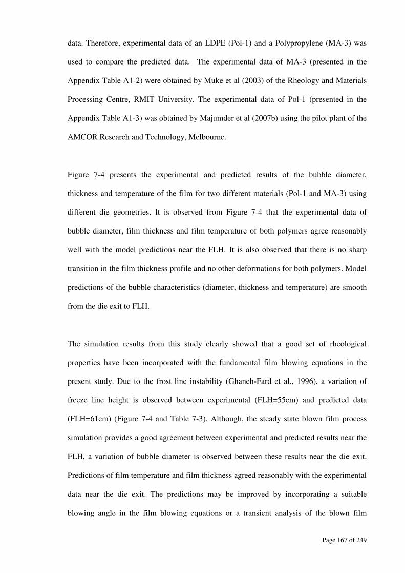
Page 167 of 249
data. Therefore, experimental data of an LDPE (Pol-1) and a Polypropylene (MA-3) was
used to compare the predicted data. The experimental data of MA-3 (presented in the
Appendix Table A1-2) were obtained by Muke et al (2003) of the Rheology and Materials
Processing Centre, RMIT University. The experimental data of Pol-1 (presented in the
Appendix Table A1-3) was obtained by Majumder et al (2007b) using the pilot plant of the
AMCOR Research and Technology, Melbourne.
Figure 7-4 presents the experimental and predicted results of the bubble diameter,
thickness and temperature of the film for two different materials (Pol-1 and MA-3) using
different die geometries. It is observed from Figure 7-4 that the experimental data of
bubble diameter, film thickness and film temperature of both polymers agree reasonably
well with the model predictions near the FLH. It is also observed that there is no sharp
transition in the film thickness profile and no other deformations for both polymers. Model
predictions of the bubble characteristics (diameter, thickness and temperature) are smooth
from the die exit to FLH.
The simulation results from this study clearly showed that a good set of rheological
properties have been incorporated with the fundamental film blowing equations in the
present study. Due to the frost line instability (Ghaneh-Fard et al., 1996), a variation of
freeze line height is observed between experimental (FLH=55cm) and predicted data
(FLH=61cm) (Figure 7-4 and Table 7-3). Although, the steady state blown film process
simulation provides a good agreement between experimental and predicted results near the
FLH, a variation of bubble diameter is observed between these results near the die exit.
Predictions of film temperature and film thickness agreed reasonably with the experimental
data near the die exit. The predictions may be improved by incorporating a suitable
blowing angle in the film blowing equations or a transient analysis of the blown film
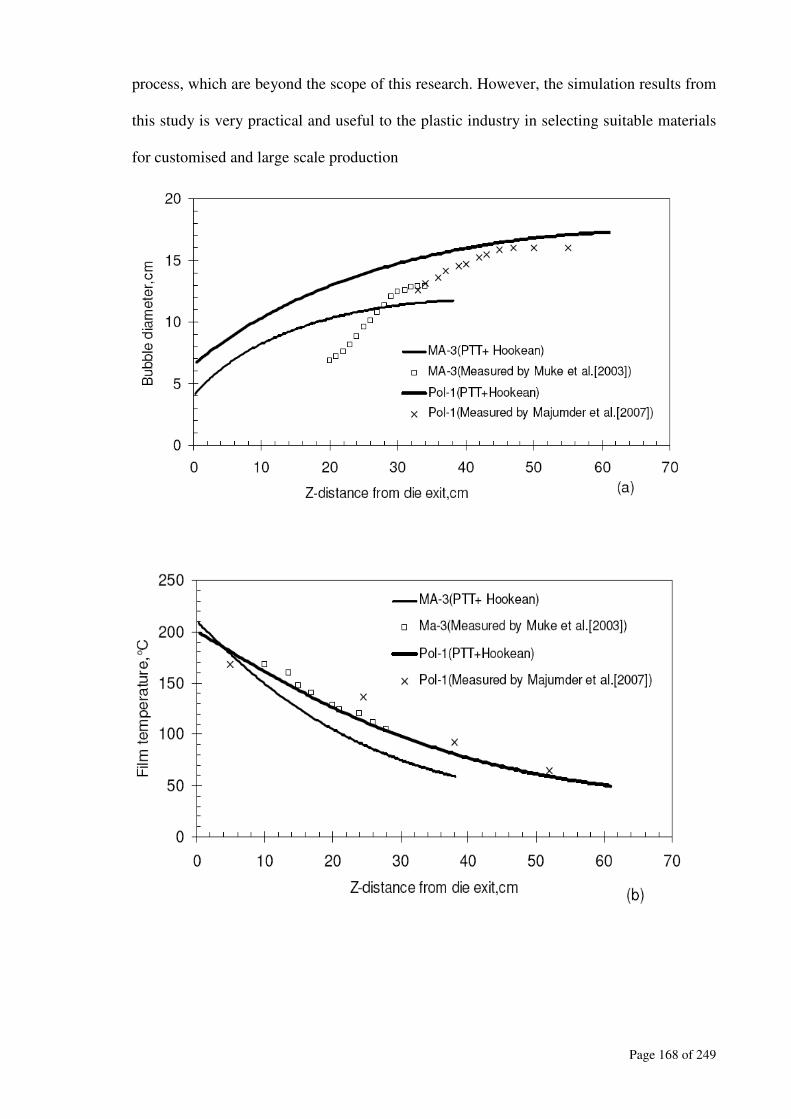
Page 168 of 249
process, which are beyond the scope of this research. However, the simulation results from
this study is very practical and useful to the plastic industry in selecting suitable materials
for customised and large scale production

Page 169 of 249
Figure 7-4: Verification of modelling outputs with the experimental data of Muke et al
(2003) and this study for-(a) bubble diameter; (b) film temperature; (c) film thickness.
Table 7-3: Comparison of the bubble characteristics of the processed film at FLH
(Majumder et al., 2007b)
At FLH Model
Prediction
Pilot plant study at
AMCOR Research
& Technology
Variation of the
experimental and model
predictions (%)
Diameter(cm) 17.3 16.03 8
Thickness(micron) 120 to 143 110 to 120 14
Temperature(°C) 59.1 65.0 9
7.3.2 Model predictions of stress and deformation rate
Figure 7-5 and 7-6 present the stress and strain rate predicted from the PTT-Hookean
model. Higher values of deformation rate and stresses are found in the machine direction in
comparison to that in the transverse direction. These values are realistic predictions in both
directions, since rates of deformation will be higher near the die exit and will diminish near
the FLH although the experimental data of stress and strain rate are not measured in this

Page 170 of 249
study. The stress in the transverse direction increases from die exit and then drops near the
FLH (Figure 7-5). The predicted rate of strain in the transverse direction is higher near the
die exit as shown in Figure 7-6 and then decreases near the FLH. Therefore, it can be
argued that near the FLH, the deformation rate in the transverse direction becomes
negligible. The prediction of the deformation rate in the machine direction (Figure 7-6) is
found to increase from die exit and then drops near the FLH. Therefore, the PTT-Hookean
model can realistically describe stress and deformation properties in the region between the
die exit and FLH. This is why the simulated results of the LDPEs (Pol-1 and MA-3) agreed
well with the experimental results as shown in Figure 7-4.
Figure 7-5: PTT-Hookean model prediction of the stresses in the machine (MD) and
transverse directions (TD) for Pol-1, respectively.

Page 171 of 249
Figure 7-6 : PTT-Hookean model prediction of the strain rate in the machine (MD) and
transverse directions (TD) for Pol-1, respectively.
7.3.3 Justification of the use of the Hookean model with the PTT
model
As discussed in the previous sections, PTT model gives better prediction when the material
is in the melt state and has branching (Hyun et al., 2004) . They found a good agreement
between their predicted and experimental results. However, the degree of long chain
branching has a significant effect on melt rheology (Majumder et al., 2007a), which will
influence the blown film process simulation. In the present study, the predictions for Pol-1
from both the PTT and the PTT-Hookean model agreed very well as shown in Figure
7-7(a) and Figure 7-7(c). However, different predictions were obtained for Pol-2 from the
PTT and the PTT-Hookean model. The extra freeze line height and bubble diameter for
Pol-2 was predicted (Figure 7-7b) from the PTT model. The thickness prediction of Pol-2
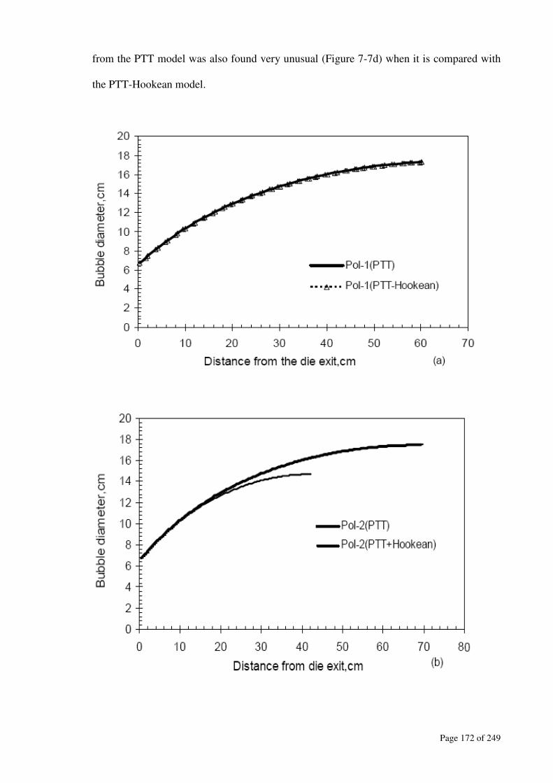
Page 172 of 249
from the PTT model was also found very unusual (Figure 7-7d) when it is compared with
the PTT-Hookean model.
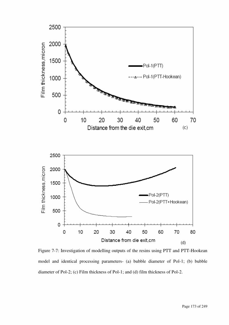
Page 173 of 249
Figure 7-7: Investigation of modelling outputs of the resins using PTT and PTT-Hookean
model and identical processing parameters- (a) bubble diameter of Pol-1; (b) bubble
diameter of Pol-2; (c) Film thickness of Pol-1; and (d) film thickness of Pol-2.
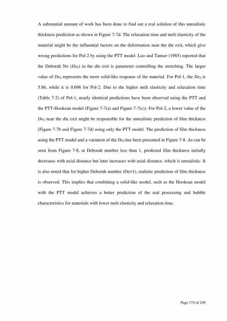
Page 174 of 249
A substantial amount of work has been done to find out a real solution of this unrealistic
thickness prediction as shown in Figure 7-7d. The relaxation time and melt elasticity of the
material might be the influential factors on the deformation near the die exit, which give
wrong predictions for Pol-2 by using the PTT model. Luo and Tanner (1985) reported that
the Deborah No (De0) in the die exit is parameter controlling the stretching. The larger
value of De0 represents the more solid-like response of the material. For Pol-1, the De0 is
5.86, while it is 0.696 for Pol-2. Due to the higher melt elasticity and relaxation time
(Table 7-2) of Pol-1, nearly identical predictions have been observed using the PTT and
the PTT-Hookean model (Figure 7-7(a) and Figure 7-7(c)). For Pol-2, a lower value of the
De0 near the die exit might be responsible for the unrealistic prediction of film thickness
(Figure 7-7b and Figure 7-7d) using only the PTT model. The prediction of film thickness
using the PTT model and a variation of the De0 has been presented in Figure 7-8. As can be
seen from Figure 7-8, at Deborah number less than 1, predicted film thickness initially
decreases with axial distance but later increases with axial distance, which is unrealistic. It
is also noted that for higher Deborah number (De>1), realistic prediction of film thickness
is observed. This implies that combining a solid-like model, such as the Hookean model
with the PTT model achieves a better prediction of the real processing and bubble
characteristics for materials with lower melt elasticity and relaxation time.

Page 175 of 249
Figure 7-8: Effect of Deborah no (De0=λv0/r0) of Pol-2 in the prediction of blown film
thickness using PTT model and present study.
7.4 Comparison study of the Kelvin and the PTT-Hookean model
Both the PTT-Hookean and the Kelvin models describe the viscoelastic properties of the
melt, although stress relaxation behaviour is predicted poorly from the Kelvin model
(Macosko, 1994). Muke et al (2003) used the Kelvin model for the blown film simulation,
which showed improved predictions compared to that using the non-isothermal Newtonian
model. In their work, a numerical integration was carried out using the assumed values of
bubble size, temperature and thickness at the FLH to trace the die exit parameters. In the
present study, die exit parameters were used as the initial conditions to solve the steady
state blown film equations until the FLH parameters are obtained which is more realistic.
Identical inputs and numerical schemes have been considered for simulation using both the
PTT-Hookean and Kelvin model.

Page 176 of 249
Predictions of the bubble diameter and film thickness from these two different models are
presented in Figure 7-9 along with the experimentally measured data (see Appendix). A
long neck of the bubble is predicted near the die exit using the Kelvin model followed by a
rapid expansion near the FLH (Figure 7-9a). This type of predictions are usually observed
for the Newtonian model as reported by Han and Park (1975a) or viscous liquid (Luo and
Tanner, 1985). A lower value of FLH is also approximated by using the Kelvin model.
Compared to the Kelvin model predictions, the bubble diameter and film thickness
predicted by the PTT-Hookean model agreed very well with the experimental data as
shown in Figure 7-9.
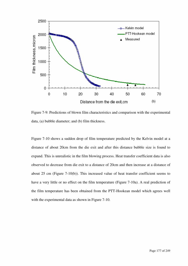
Page 177 of 249
Figure 7-9: Predictions of blown film characteristics and comparison with the experimental
data, (a) bubble diameter; and (b) film thickness.
Figure 7-10 shows a sudden drop of film temperature predicted by the Kelvin model at a
distance of about 20cm from the die exit and after this distance bubble size is found to
expand. This is unrealistic in the film blowing process. Heat transfer coefficient data is also
observed to decrease from die exit to a distance of 20cm and then increase at a distance of
about 25 cm (Figure 7-10(b)). This increased value of heat transfer coefficient seems to
have a very little or no effect on the film temperature (Figure 7-10a). A real prediction of
the film temperature has been obtained from the PTT-Hookean model which agrees well
with the experimental data as shown in Figure 7-10.
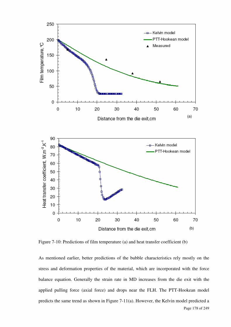
Page 178 of 249
Figure 7-10: Predictions of film temperature (a) and heat transfer coefficient (b)
As mentioned earlier, better predictions of the bubble characteristics rely mostly on the
stress and deformation properties of the material, which are incorporated with the force
balance equation. Generally the strain rate in MD increases from the die exit with the
applied pulling force (axial force) and drops near the FLH. The PTT-Hookean model
predicts the same trend as shown in Figure 7-11(a). However, the Kelvin model predicted a

Page 179 of 249
decreased strain rate in MD from the die exit for a distance of about 15cm and then
increased after that point. A lower value of strain rate is also predicted from the Kelvin
model in both MD and TD in comparison to the PTT-Hookean model.
The long neck in the bubble diameter near the die exit predicted from the Kelvin model
may be due this lower value of deformation rate. The strain rates in both directions may be
nullified also to predict this long neck. This distance (15cm from the die exit) predicted
from the Kelvin model can be termed as the critical distance which is absent in the PTT-
Hookean model.
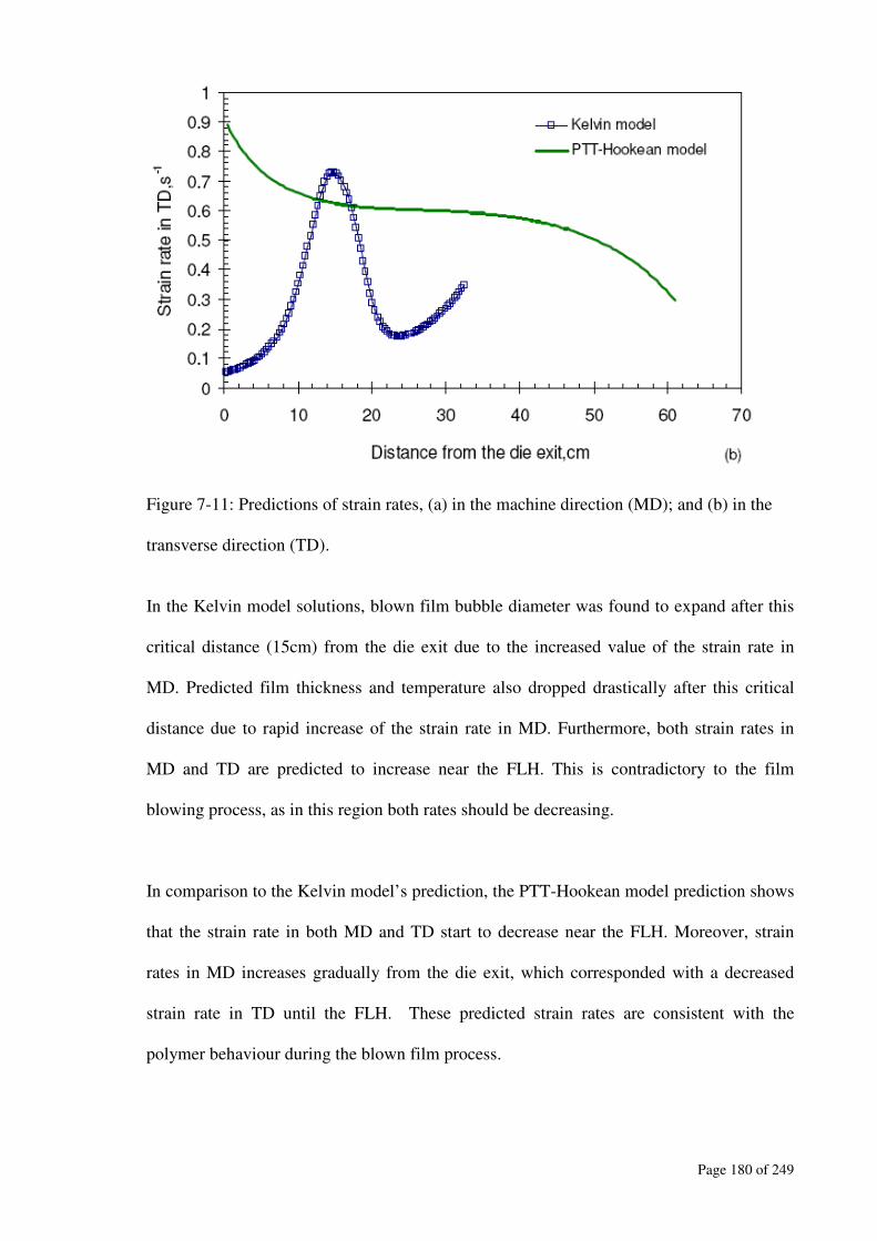
Page 180 of 249
Figure 7-11: Predictions of strain rates, (a) in the machine direction (MD); and (b) in the
transverse direction (TD).
In the Kelvin model solutions, blown film bubble diameter was found to expand after this
critical distance (15cm) from the die exit due to the increased value of the strain rate in
MD. Predicted film thickness and temperature also dropped drastically after this critical
distance due to rapid increase of the strain rate in MD. Furthermore, both strain rates in
MD and TD are predicted to increase near the FLH. This is contradictory to the film
blowing process, as in this region both rates should be decreasing.
In comparison to the Kelvin model’s prediction, the PTT-Hookean model prediction shows
that the strain rate in both MD and TD start to decrease near the FLH. Moreover, strain
rates in MD increases gradually from the die exit, which corresponded with a decreased
strain rate in TD until the FLH. These predicted strain rates are consistent with the
polymer behaviour during the blown film process.
Page 181 of 249
Dynamic or transient solutions are usually more accurate for any dynamic process like
blown film extrusion. However, these techniques are difficult to solve due to the
involvement of a lot of numerical complexity to consider all dynamic instabilities during
processing. Steady state solutions are simple, quick and provide reasonable predictions for
engineering needs. Therefore, this study is focussed to steady state solution of the blown
film process to obtain the process and bubble characteristics with a reasonable accuracy.
7.5 Summary
Based on present and some earlier study, it is revealed that a suitable rheological equation
is important to get better predictions from the blown film modelling. Considering all
viscoelastic models (PTT, PTT-Hookean and Kelvin) presented here, the PTT-Hookean
model provides most reasonable predictions about FLH, bubble diameter, film thickness
and film temperature. The accuracy between the PTT-Hookean model predictions and
experimental data is about 10%, which is reasonable for engineering needs. The PTT-
Hookean model is also more suitable for the materials of lower melt elasticity and
relaxation time. The key findings of this modelling (PTT-Hookean) study are:
Realistic profile of bubble characteristics(diameter, thickness and temperature)
Predictions of freezing line height using the die exit data
Reasonable agreement of the model prediction with the present (using Pol-1) and
earlier study (Muke et al., 2003) using different materials and die geometry
These types of prediction (FLH and bubble characteristics of the blown film) are useful to
the blown film industry when new materials are used. This technique can reduce or avoid
costly trial runs.
Page 182 of 249
CHAPTER : 8
Statistical Analysis of the Film Properties
This chapter presents the statistical analysis of the blown film properties obtained at
different process variables such as die temperature and cooling rate. Mechanical and
optical properties of the blown film have also been discussed with respect to their
molecular structure. For each film property, a summary table has been provided with
respect to the effect of die temperature, cooling rate and combination of both. This
analysis will provide useful information to optimise the film properties of the two LDPEs
used in this study.
8.1 Basis of the statistical analysis
The effect of the process variables on the blown films have been determined statistically
using commercial software (MINITAB-14). Confidence level was set at 95% for all runs.
The interaction plots, which include both the main effects (the effect of a factor on the
dependent variable (response) measured without regard to other factors in the analysis)
and 2-factor interactions, have been presented here for both LDPEs. Pareto charts (a bar
graph used to arrange information in such a way that priorities for process improvement
can be established) were used to compare the relative magnitude and the statistical
significance of both main (temperature and cooling rate) variables. These Pareto charts are
presented in the Appendix (Figures A3-1 to A3-12). MINITAB plots the effects in
decreasing order of the absolute value of the standardized effects and draws a reference
line on the Pareto chart. Any effect that extends past this reference line is significant.
Normal probability analysis was also performed to determine the negative or positive
effects of temperature and cooling rate on the film properties and presented in the
Appendix (Figures A3-13 to A3-17). If the effect of a processing variable like temperature
Page 183 of 249
or cooling rate becomes significant and positive, it means that with the increase of that
processing variable, the particular film properties will be increased and vice versa.
8.2 Mechanical properties
8.2.1 Tensile strength
It is assumed that the undeformed polymer has crystals, which are stacked molecules in a
regular manner. During the tensile testing, the crystals start to crack and chains are pulled
out. At sufficiently high strain the molecules and crystal blocks become aligned parallel to
the stretching direction and a fibrillar structure is formed.
From the rheological information, it is clear that zero shear viscosity of Pol-1 is higher than
Pol-2 (Figure 6-7 and Tables 6-2 and 6-3), which is reflected in tensile strength (Figure 8-1
and 8-2). For Pol-2, chain ends and low molecular weight material in the inter-lamellar
region may be responsible for reducing the number of tie molecules and tensile strength.
No direct relationship between molecular weight and the tensile properties was identified.
However, it is known that the molecular weight affects the crystalline properties (e.g.,
lamellar thickness, spherulite size and degree of crystallinity) and chain entanglements in
the amorphous region (Nielson L.E., 1993).
From the Pareto chart (Appendix Figure A3-1a), it is obvious that the combined effect of
temperature and cooling is higher on the tensile strength of Pol-1 in the machine direction.
For Pol-2 combined effect of both die temperature and cooling rate is significant on the
film tensile strength (Table 8-1). It is also shown for Pol-2 (Appendix Figure A3-2) that
temperature effect is more significant than the cooling effect for tensile strength in the
machine direction. The crystalline properties of the resin also show that the temperature
effect is higher than the cooling effect (Tables 5-7 and 8-2). For the tensile strength in
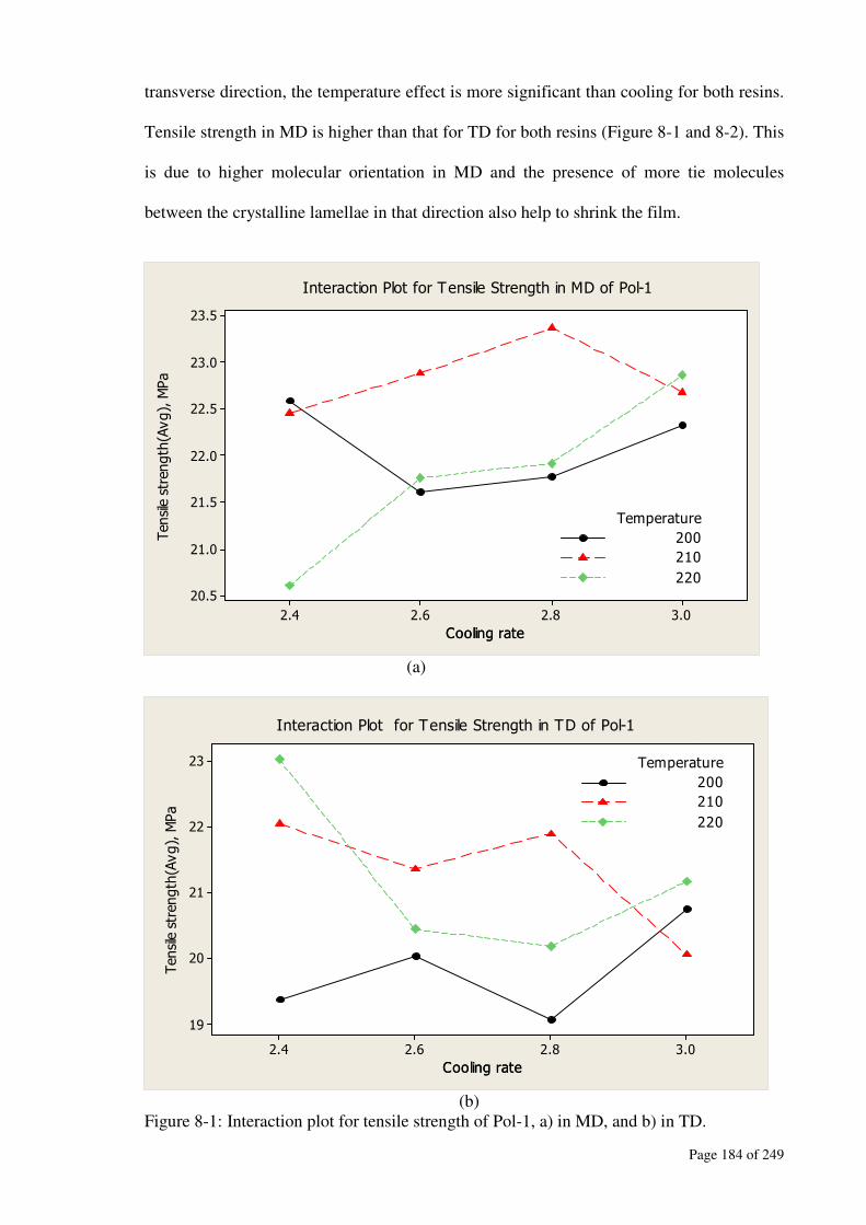
Page 184 of 249
transverse direction, the temperature effect is more significant than cooling for both resins.
Tensile strength in MD is higher than that for TD for both resins (Figure 8-1 and 8-2). This
is due to higher molecular orientation in MD and the presence of more tie molecules
between the crystalline lamellae in that direction also help to shrink the film.
Cooling rateCooling rate
Tensile strength(Avg), MPa
3.02.82.62.4
23.5
23.0
22.5
22.0
21.5
21.0
20.5
Temperature
220
200
210
Interaction Plot for Tensile Strength in MD of Pol-1
(a)
Cooling rateCooling rate
Tensile strength(Avg), MPa
3.02.82.62.4
23
22
21
20
19
Temperature
220
200
210
Interaction Plot for Tensile Strength in TD of Pol-1
(b)
Figure 8-1: Interaction plot for tensile strength of Pol-1, a) in MD, and b) in TD.
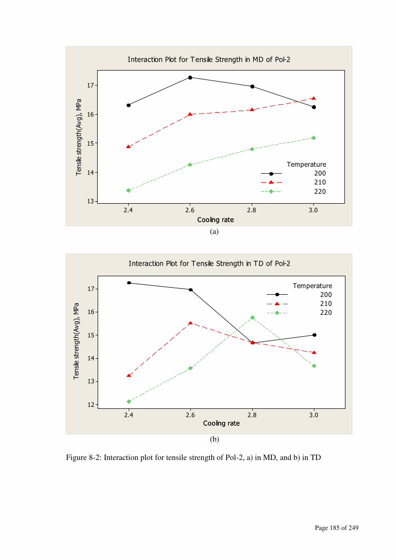
Page 185 of 249
Cooling rateCooling rate
Tensile strength(Avg), MPa
3.02.82.62.4
17
16
15
14
13
Temperature
220
200
210
Interaction Plot for Tensile Strength in MD of Pol-2
(a)
Cooling rateCooling rate
Tensile strength(Avg), MPa
3.02.82.62.4
17
16
15
14
13
12
Temperature
220
200
210
Interaction Plot for Tensile Strength in TD of Pol-2
(b)
Figure 8-2: Interaction plot for tensile strength of Pol-2, a) in MD, and b) in TD

Page 186 of 249
Table 8-1: Effect of temperature and cooling rate on the tensile strength (Appendix Figure
A3-13)
Stretching
direction
Resins Temperature Cooling rate Temperature and
cooling rate
Machine Pol-1 Not significant Not significant Not significant
Machine Pol-2 Significant and
negative
Significant and
positive
Significant and
positive
Transverse Pol-1 Not significant Not significant Not significant
Transverse Pol-2 Significant and
negative
Not significant Significant and
positive
Table 8-2: Crystalline properties of the blown films at 210°C (die temperature)
Blower Setting Heat of Fusion(J/g) % Crystallinity
Pol-1 Pol-2 Pol-1 Pol-2
2.4 113.5 111.9 63.03 62.14
2.6 112.9 107.5 62.73 59.70
2.8 103.8 102.4 57.69 56.87
3.0 100.6 99.88 55.87 55.49
8.2.2 Tear strength
Tear strength determines the energy necessary to propagate a tear in the film. In the tearing
process, the predominant mechanism is the breaking of chains. The surfaces of the tear
cracks are rough on a molecular scale since the tear follows a path of least resistance to
minimize the number of chains that are broken.
The tear strength of Pol-1 (Figure 8-3) gives similar values in both directions (MD and
TD), whereas Pol-2 has a significantly higher value in TD compared to that in MD (Figure
8-4). The variation of tear strength resulted from their variation of zero shear viscosity,
long chain branching and longer relaxation time in Pol-1 (Chapter 6) responsible for highly
oriented fibrillar nuclei to promote the row-nucleated structure over the spherulites (Zhang,
2004). At higher cooling rate (BS=3.0), Pol-1 shows higher tear strength in machine
direction (Figure 8-3) because of its long chain backbone, higher degree of LCB and
longer relaxation time, which supports the lower degree of chain alignment in the direction

Page 187 of 249
of flow and the capacity to form interlamellar links which allows the lamellae to be
separated and hence the films torn easily along TD. Pol-2 with lower degree of LCB is able
to extend in response to the extensional flow during film blowing and thus form tie
molecules more readily, showing high resistance to tearing along TD. Therefore, Pol-2
shows higher tear strength in TD than in MD. However, tear strength of Pol-1 is higher
than Pol-2 in both directions (Figures 8-3 and 8-4) due to its higher zero shear viscosity
which has resulted from higher degree of entanglement. For Pol-1 and Pol-2, tear strength
decreases with the increased temperature, as tearing energy increases with damping factor
(loss modulus(G”)/storage modulus(G’))(Nielson L.E., 1993) .
For the tear strength of Pol-1, die temperature effect is more significant than the cooling
rate in both directions (Appendix Figure A3-3), whereas cooling effect is more significant
for Pol-2 (Appendix Figure A3-4). At higher temperature, molecular orientation is changed
and the chains are extended, so tear strength is less in both directions. For both resins,
higher cooling rate is favourable for better tear strength (Figures 8-3 and 8-4 and Table
8-3).

Page 188 of 249
Cooling rateCooling rate
Tear strength(Avg), m
N
3.02.82.62.4
600
500
400
300
200
Temperature
220
200
210
Interaction Plot for Tear Strength in MD of Pol-1
(a)
Cooling rateCooling rate
Tear strength(Avg), m
N
3.02.82.62.4
440
420
400
380
360
340
320
Temperature
220
200
210
Interaction Plot for Tear Strength in TD of Pol-1
(b)
Figure 8-3: Interaction plot for tear strength of Pol-1, a) in MD, and b) in TD..

Page 189 of 249
Cooling rateCooling rate
Tear Strength(Avg),mN
3.02.82.62.4
240
230
220
210
200
190
180
170
Temperature
220
200
210
Interaction Plot (data means) for Tear strength in MD of Pol-2
(a)
Cooling rateCooling rate
Tear strength(Avg), m
N
3.02.82.62.4
380
370
360
350
340
330
320
310
300
Temperature
220
200
210
Interaction Plot for Tear Strength in TD of Pol-2
(b)
Figure 8-4: Interaction plot for tear strength of Pol-2, a) in MD, and b) in TD.
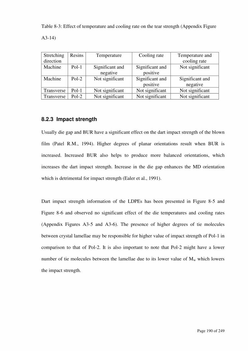
Page 190 of 249
Table 8-3: Effect of temperature and cooling rate on the tear strength (Appendix Figure
A3-14)
Stretching
direction
Resins Temperature Cooling rate Temperature and
cooling rate
Machine Pol-1 Significant and
negative
Significant and
positive
Not significant
Machine Pol-2 Not significant Significant and
positive
Significant and
negative
Transverse Pol-1 Not significant Not significant Not significant
Transverse Pol-2 Not significant Not significant Not significant
8.2.3 Impact strength
Usually die gap and BUR have a significant effect on the dart impact strength of the blown
film (Patel R.M., 1994). Higher degrees of planar orientations result when BUR is
increased. Increased BUR also helps to produce more balanced orientations, which
increases the dart impact strength. Increase in the die gap enhances the MD orientation
which is detrimental for impact strength (Ealer et al., 1991).
Dart impact strength information of the LDPEs has been presented in Figure 8-5 and
Figure 8-6 and observed no significant effect of the die temperatures and cooling rates
(Appendix Figures A3-5 and A3-6). The presence of higher degrees of tie molecules
between crystal lamellae may be responsible for higher value of impact strength of Pol-1 in
comparison to that of Pol-2. It is also important to note that Pol-2 might have a lower
number of tie molecules between the lamellae due to its lower value of Mw which lowers
the impact strength.
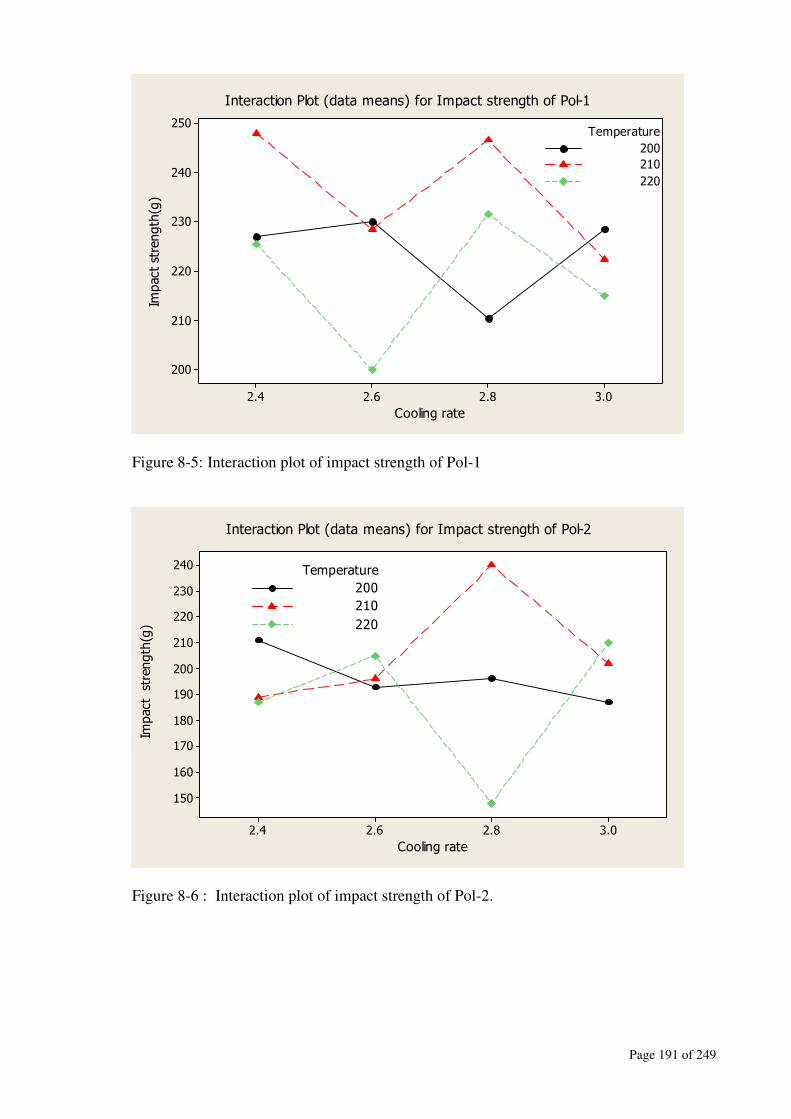
Page 191 of 249
Cooling rate
Impact strength(g)
3.02.82.62.4
250
240
230
220
210
200
Temperature
220
200
210
Interaction Plot (data means) for Impact strength of Pol-1
Figure 8-5: Interaction plot of impact strength of Pol-1
Cooling rate
Impact strength(g)
3.02.82.62.4
240
230
220
210
200
190
180
170
160
150
Temperature
220
200
210
Interaction Plot (data means) for Impact strength of Pol-2
Figure 8-6 : Interaction plot of impact strength of Pol-2.

Page 192 of 249
8.3 Shrinkage properties
Thermal shrinkage is a measure of chain extension in the amorphous phase. This is
considered to happen mainly due to the relaxation of extended and oriented tie chains
locked in by crystallites. The tie chains between crystalline lamellae account for a large
portion of the amorphous material. Therefore, the orientation of crystallites might have a
large effect on the amorphous phase orientation.
From the rheological data, it is found that relaxation time of Pol-1 is higher than Pol-2
(Chapter 6) due to its long chain backbone and higher degree of LCB characteristics for
entanglements. These entanglement properties are behaving as temporary crosslink which
can be extended by stretching in the molten state. Pol-1 with higher degree of LCB
characteristics shows higher shrinkage than Pol-2 (Figure 8-7 and 8-8) due to its higher
amorphous orientation and chain extension frozen into the film by stresses during
deformation. Also due to the narrow molecular weight distribution, Pol-2 may contain
loose loops or chain ends which have relatively low contribution towards shrinkage.
MD shrinkage is always higher than TD shrinkage due to the preferred orientation of the
amorphous chain segments (tie molecules) in that direction. The effect of temperature and
cooling rate on the shrinkage in MD is significant for both resins (Appendix Figures A3-7
and A3-8 and Table 8-4). For the shrinkage properties in MD, temperature effect was
found to be more significant than the cooling effect. Like tear strength, low temperature
and high cooling rate are suitable for greater shrinkage in MD (Figure 8-7a and 8-8 and
Table 8-4) due to the lower degree of crystallinity experienced at this condition.
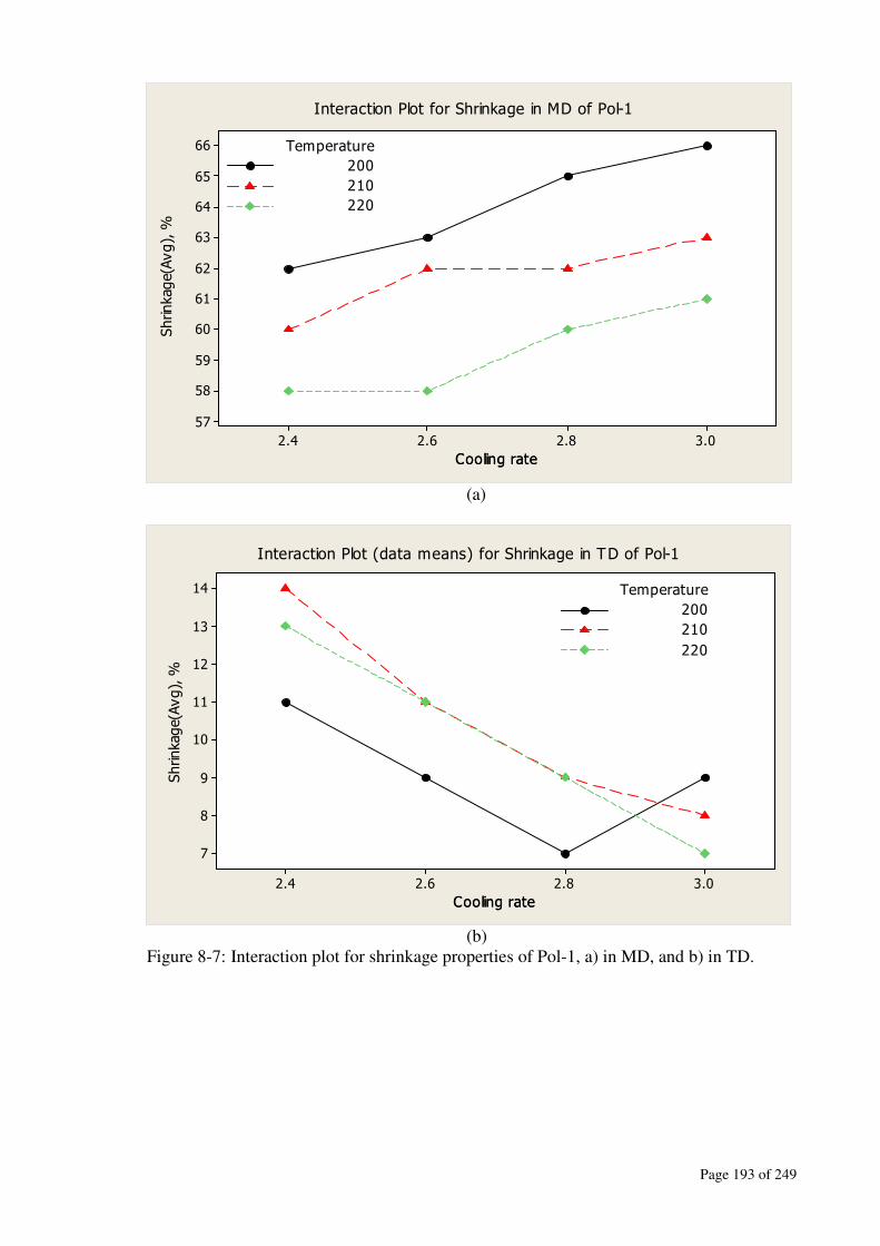
Page 193 of 249
Cooling rateCooling rate
Shrinkage(Avg), %
3.02.82.62.4
66
65
64
63
62
61
60
59
58
57
Temperature
220
200
210
Interaction Plot for Shrinkage in MD of Pol-1
(a)
Cooling rateCooling rate
Shrinkage(Avg), %
3.02.82.62.4
14
13
12
11
10
9
8
7
Temperature
220
200
210
Interaction Plot (data means) for Shrinkage in TD of Pol-1
(b)
Figure 8-7: Interaction plot for shrinkage properties of Pol-1, a) in MD, and b) in TD.
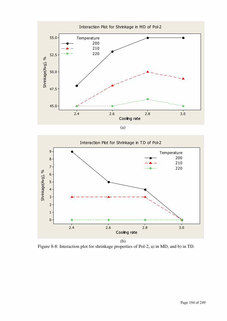
Page 194 of 249
Cooling rateCooling rate
Shrinkage(Avg), %
3.02.82.62.4
55.0
52.5
50.0
47.5
45.0
Temperature
220
200
210
Interaction Plot for Shrinkage in MD of Pol-2
(a)
Cooling rateCooling rate
Shrinkage(Avg), %
3.02.82.62.4
9
8
7
6
5
4
3
2
1
0
Temperature
220
200
210
Interaction Plot for Shrinkage in TD of Pol-2
(b)
Figure 8-8: Interaction plot for shrinkage properties of Pol-2, a) in MD, and b) in TD.
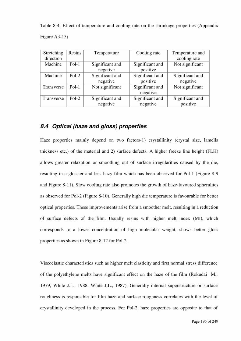
Page 195 of 249
Table 8-4: Effect of temperature and cooling rate on the shrinkage properties (Appendix
Figure A3-15)
Stretching
direction
Resins Temperature Cooling rate Temperature and
cooling rate
Machine Pol-1 Significant and
negative
Significant and
positive
Not significant
Machine Pol-2 Significant and
negative
Significant and
positive
Significant and
negative
Transverse Pol-1 Not significant Significant and
negative
Not significant
Transverse Pol-2 Significant and
negative
Significant and
negative
Significant and
positive
8.4 Optical (haze and gloss) properties
Haze properties mainly depend on two factors-1) crystallinity (crystal size, lamella
thickness etc.) of the material and 2) surface defects. A higher freeze line height (FLH)
allows greater relaxation or smoothing out of surface irregularities caused by the die,
resulting in a glossier and less hazy film which has been observed for Pol-1 (Figure 8-9
and Figure 8-11). Slow cooling rate also promotes the growth of haze-favoured spherulites
as observed for Pol-2 (Figure 8-10). Generally high die temperature is favourable for better
optical properties. These improvements arise from a smoother melt, resulting in a reduction
of surface defects of the film. Usually resins with higher melt index (MI), which
corresponds to a lower concentration of high molecular weight, shows better gloss
properties as shown in Figure 8-12 for Pol-2.
Viscoelastic characteristics such as higher melt elasticity and first normal stress difference
of the polyethylene melts have significant effect on the haze of the film (Rokudai M.,
1979, White J.L., 1988, White J.L., 1987). Generally internal superstructure or surface
roughness is responsible for film haze and surface roughness correlates with the level of
crystallinity developed in the process. For Pol-2, haze properties are opposite to that of
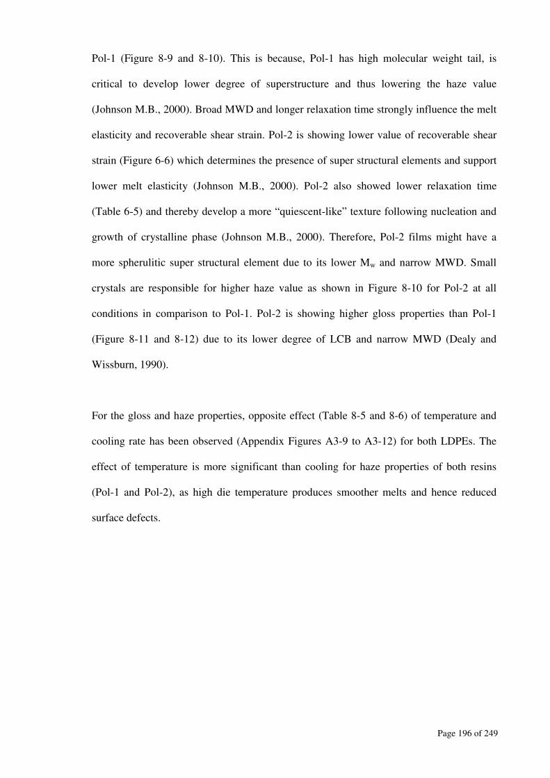
Page 196 of 249
Pol-1 (Figure 8-9 and 8-10). This is because, Pol-1 has high molecular weight tail, is
critical to develop lower degree of superstructure and thus lowering the haze value
(Johnson M.B., 2000). Broad MWD and longer relaxation time strongly influence the melt
elasticity and recoverable shear strain. Pol-2 is showing lower value of recoverable shear
strain (Figure 6-6) which determines the presence of super structural elements and support
lower melt elasticity (Johnson M.B., 2000). Pol-2 also showed lower relaxation time
(Table 6-5) and thereby develop a more “quiescent-like” texture following nucleation and
growth of crystalline phase (Johnson M.B., 2000). Therefore, Pol-2 films might have a
more spherulitic super structural element due to its lower Mw and narrow MWD. Small
crystals are responsible for higher haze value as shown in Figure 8-10 for Pol-2 at all
conditions in comparison to Pol-1. Pol-2 is showing higher gloss properties than Pol-1
(Figure 8-11 and 8-12) due to its lower degree of LCB and narrow MWD (Dealy and
Wissburn, 1990).
For the gloss and haze properties, opposite effect (Table 8-5 and 8-6) of temperature and
cooling rate has been observed (Appendix Figures A3-9 to A3-12) for both LDPEs. The
effect of temperature is more significant than cooling for haze properties of both resins
(Pol-1 and Pol-2), as high die temperature produces smoother melts and hence reduced
surface defects.
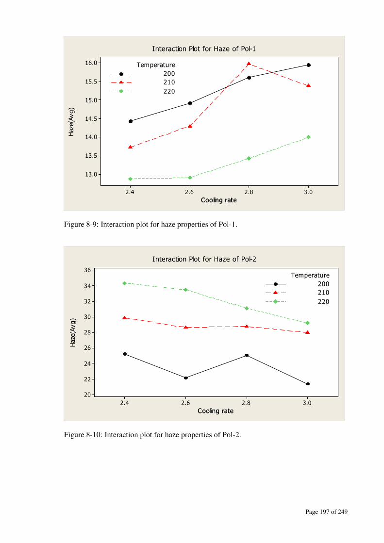
Page 197 of 249
Cooling rateCooling rate
Haze(Avg)
3.02.82.62.4
16.0
15.5
15.0
14.5
14.0
13.5
13.0
Temperature
220
200
210
Interaction Plot for Haze of Pol-1
Figure 8-9: Interaction plot for haze properties of Pol-1.
Cooling rateCooling rate
Haze(Avg)
3.02.82.62.4
36
34
32
30
28
26
24
22
20
Temperature
220
200
210
Interaction Plot for Haze of Pol-2
Figure 8-10: Interaction plot for haze properties of Pol-2.
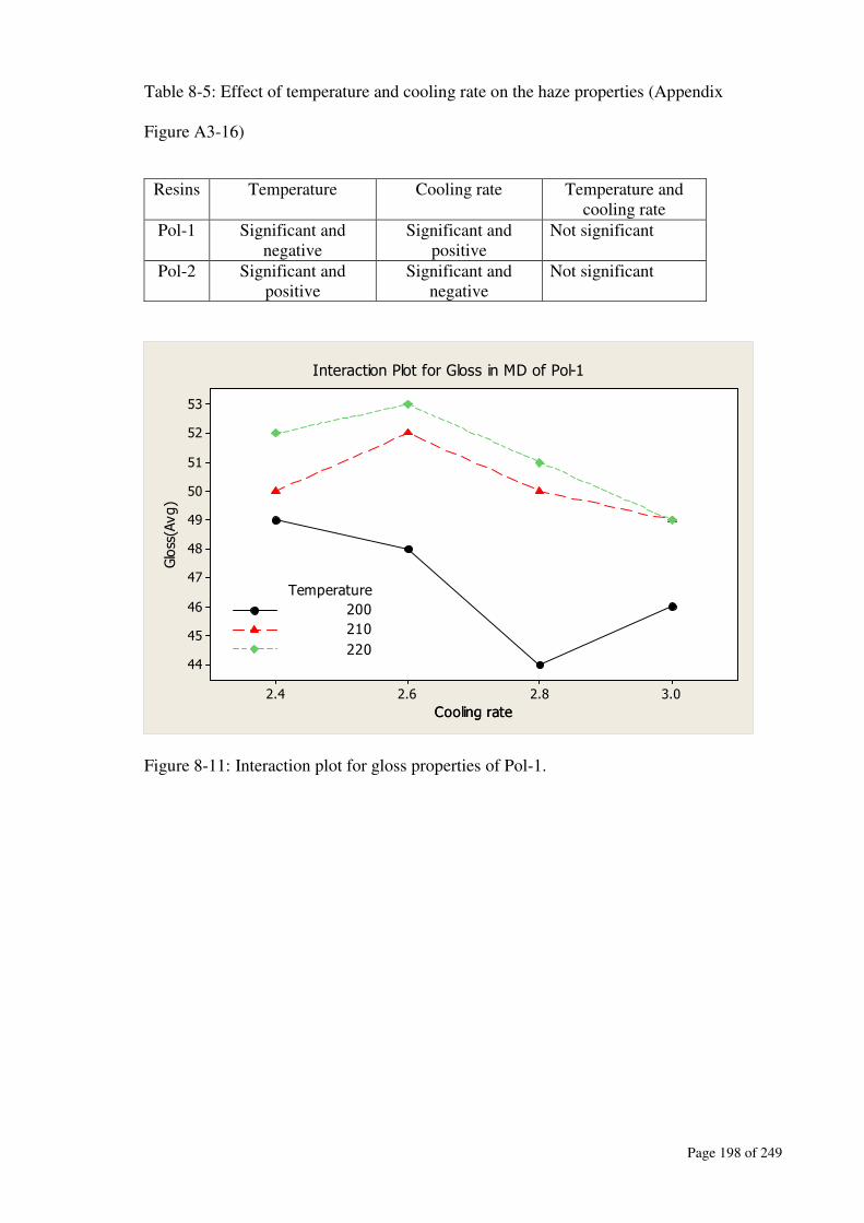
Page 198 of 249
Table 8-5: Effect of temperature and cooling rate on the haze properties (Appendix
Figure A3-16)
Resins Temperature Cooling rate Temperature and
cooling rate
Pol-1 Significant and
negative
Significant and
positive
Not significant
Pol-2 Significant and
positive
Significant and
negative
Not significant
Cooling rateCooling rate
Gloss(Avg)
3.02.82.62.4
53
52
51
50
49
48
47
46
45
44
Temperature
220
200
210
Interaction Plot for Gloss in MD of Pol-1
Figure 8-11: Interaction plot for gloss properties of Pol-1.
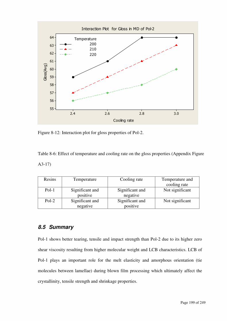
Page 199 of 249
Cooling rate
Gloss(Avg)
3.02.82.62.4
64
63
62
61
60
59
58
57
56
55
Temperature
220
200
210
Interaction Plot for Gloss in MD of Pol-2
Figure 8-12: Interaction plot for gloss properties of Pol-2.
Table 8-6: Effect of temperature and cooling rate on the gloss properties (Appendix Figure
A3-17)
Resins Temperature Cooling rate Temperature and
cooling rate
Pol-1 Significant and
positive
Significant and
negative
Not significant
Pol-2 Significant and
negative
Significant and
positive
Not significant
8.5 Summary
Pol-1 shows better tearing, tensile and impact strength than Pol-2 due to its higher zero
shear viscosity resulting from higher molecular weight and LCB characteristics. LCB of
Pol-1 plays an important role for the melt elasticity and amorphous orientation (tie
molecules between lamellae) during blown film processing which ultimately affect the
crystallinity, tensile strength and shrinkage properties.

Page 200 of 249
Higher haze value of Pol-2 is due to the presence of smaller crystal size and
superstructures, which is the main reason for surface defects. Low haze value of Pol-1 is
due to its high molecular weight tail which inhibits the development of more
superstructures. Higher gloss properties of Pol-2 are due to its narrow MWD. At low
cooling rates, polymer molecules have more opportunity to position themselves closer
together resulting higher crystallinity.
High temperature and low cooling rate are favourable for low haze and high gloss
properties. Pol-1 shows higher shrinkage properties due to its higher relaxation time and
more amorphous orientation originated from long chain branching. For Pol-1 and Pol-2,
gloss and haze properties are just opposite due to their different melt flow behaviour
resulting from their molecular characteristics. For Pol-1 and Pol-2, low temperature and
high cooling rate are suitable for both tear and shrinkage properties because at low
temperature and high cooling rate, chains are entangled with higher amorphous
orientation.
Statistical analysis showed that temperature has more significant effect than the cooling
rate on the finished LDPE film properties because at higher temperature molecular
orientation is changed and the chains are already extended. Cooling rate is important
mainly to control the crystallinity and the bubble stability. Nonlinear film properties have
been obtained due to the non-isothermal melt flow and die swelling which affects the
spacing between the atomic planes in the films observed in WAXD analysis.
Page 201 of 249
CHAPTER : 9
Conclusions and Recommendations
The important conclusions of this research are presented in the following sections:
9.1 Rheological properties
The rheological studies of the LDPEs conclude that:
• Pol-1 provides higher zero shear viscosity (ZSV) and relaxation time in comparison
to Pol-2 due to its higher molecular weight and long chain branching (LCB)
characteristics. Higher ZSV indicates higher mechanical properties of the film.
• Pol-2 shows lower value of melt elasticity, related to short relaxation time, which
will promote more spherulitic-like superstructural element in the film. Film haze
property will increase with the higher values of spherulitic-like superstructure.
Higher die temperature is used to improve optical properties(less hazy) of the blown
film. Lower melt elasticity of Pol-2 also limits its blown film processability at higher
die temperatures due to the lower melt strength leading to bubble instability.
• Pol-1 shows higher degree of shear thinning due to its broad MWD and higher
degree of LCB.
• Pol-1 shows higher extensional viscosity and strain hardening in comparison to that
for Pol-2 due to the higher values of molecular weight and higher degree of LCB.
Based on the measured rheological properties of two LDPEs, it can be argued that Pol-1 is
more suitable in the film blowing process than Pol-2.

Page 202 of 249
9.2 Crystalline properties
Sharp crystalline peaks and narrow crystal size distribution of Pol-2 were obtained from
both WAXD and MDSC studies due to the absence of any high molecular weight chain.
These sharp crystalline peaks and small crystal size are detrimental for film haze properties.
For Pol-1, long branched molecules participated in the crystallization process along with the
main chain, producing more crystallinity than Pol-2. That is why higher crystallinity is
reported for Pol-1 and its films obtained at different cooling rates. Film crystallinity is also
found to increase with the cooling rates for both LDPEs.
9.3 Blown film modelling and simulation
The following conclusions can be drawn from the numerical analysis of the blown film
processing:
• A new rheological constitutive equation is established by combining the Phan-
Thien and Tanner model and the Hookean model. This new constitutive equation is
reported here as the PTT-Hookean model.
• Using the PTT-Hookean model, simulation of a steady state blown film process
gave bubble characteristics and freeze line height with a reasonable accuracy.
• The variation between the PTT-Hookean model predictions and experimental data
is about 10%, which is reasonable for engineering needs.
• The PTT-Hookean model is also more suitable for the materials of lower melt
elasticity and relaxation time.
• The key findings of this modelling (PTT-Hookean) and simulation are-
Realistic profile of bubble characteristics (diameter, thickness and
temperature)
Predictions of freezing line height using the die exit data
Page 203 of 249
Reasonable agreement of the predicted value with the present (using Pol-1)
and previous study (Muke et al., 2003) using different materials and die geometry
These types of predictions (FLH and bubble characteristics of the blown film) are useful to
the polymeric film industry to develop suitable materials for blown film extrusion with
desirable film properties. This simulation is simple and robust in predicting the bubble
characteristics quickly to meet the engineering need.
9.4 Blown film properties
It has been observed from the experimental data of blown film properties that Pol-1 film
has better tear, tensile and impact strength than Pol-2 due to its higher zero shear viscosity
resulting from higher molecular weight chain and LCB characteristics. Higher haze value
of Pol-2 was due to the presence of smaller crystal size and superstructures which is also
the main reason for surface defects. Low haze value of Pol-1 was obtained due to its high
molecular weight tail leading to more superstructures. Higher gloss properties of Pol-2
were obtained for its narrow MWD. At low cooling rates, polymer molecules have more
opportunity to position themselves closer together resulting in higher crystallinity.
High temperature and low cooling rate are favourable for low haze and high gloss
properties. Pol-1 shows higher shrinkage properties due to its higher relaxation time and
more amorphous orientation originated from long chain branching. For Pol-1 and Pol-2
gloss and haze properties are just opposite due to their different melt flow behaviour
resulting from their molecular characteristics. For Pol-1 and Pol-2, low temperature and
high cooling rate are suitable for both tear and shrinkage properties, because at low
temperature and high cooling rate, chains are entangled with higher amorphous orientation.

Page 204 of 249
Nonlinear relationship of the film strength with the cooling rates in blown film process
properties has been obtained due to the non-isothermal melt flow and melt elasticity, which
affect the spacing between the molecules in the films as observed in WAXD analysis.
Based on the rheological, thermal and crystalline properties, it can be argued that LCB plays
an important role in melt rheology and amorphous orientation (tie molecules between
lamellae) during blown film processing, which ultimately affects film crystallinity and film
properties.
9.5 Recommendations for future work
The variation between experimental and predicted data is about 10%. This variation can be
minimised by using the current governing equations for blown film simulation and by
considering the following suggestions:
• A transient solution of the blown film process considering film crystallinity and all
process dynamics such as bubble instability, freeze line height variation etc should
be attempted.
• This study incorporates the effect of temperature difference between the film
surfaces, velocity of the cooling air and radius of the bubble on the heat transfer
coefficient. However, end effect of the cooling air at the lip of the die exit and after
the FLH are also important and needs to be considered for further study in this
area.
• Die swell and gravity effects can also be considered
Page 205 of 249
Bibliography
ABHIRAMAN, A. S. (2003) Shish Kebab and High Performance Morphologies. J.
Applied Polymer Science, 23, 2419.
ALAIE, S. M. & PAPANASTASIOU, T. C. (1993) Modelling of non-Isothermal film
blowing with integarl constitutive equations. Int. Polym. Process, 8, 51-65.
ALEXANDER, L. (1969) X-ray diffraction methods in polymer science, Wiley-
Interscience.
ALLEN, V. & FOX, T. (1964) Viscosity—Molecular Weight Dependence for Short Chain
Polystyrenes. The Journal of Chemical Physics, 41, 344.
BAFNA, A., BEAUCAGE G., MIRABELLA F. & SUKUMARAN S. (2001) Optical
Properties and Orientation in Polyethylene Blown Films. J. Polymer Science, 39,
2923-2936.
BAGLEY, E. & SCHREIBER, H. (1961) Effect of Die Entry Geometry on Polymer Melt
Fracture and Extrudate Distortion. Journal of Rheology, 5, 341.
BAIRD, D. (1999) The role of extensional rheology in polymer processing. Korea-
Australia Rheology Journal, 11, 305-311.
BAKER, A. & WINDLE, A. (2001) Evidence for a partially ordered component in
polyethylene from wide-angle X-ray diffraction. Polymer, 42, 667-680.
BALKE, S. (1984) Quantitative column liquid chromatography, Elsevier New York.
BALLMAN, R. (1965) Extensional flow of polystyrene melt. Rheologica Acta, 4, 137-140.
BARROSO, V., COVAS, J. & MAIA, J. (2002) Sources of error and other difficulties in
extensional rheometry revisited: commenting and complementing a recent paper by
T. Schweizer. Rheologica Acta, 41, 154-161.
BENNETT, J. C. & SHEPHERD, J. J. (2006) Analysis of the non-isothermal Newtonian
model in the blown film process. ANZIAM J., 47, 325-338.
BOOIJ, H. & PALMEN, J. (1982) Some aspects of linear and nonlinear viscoelastic
behaviour of polymer melts in shear. Rheologica Acta, 21, 376-387.
BUSSE, W. & LONGWORTH, R. (1962) Effect of molecular weight distribution and
branching on the viscosity of polyethylene melts. Journal of Polymer Science, 58,
49-69.
CAIN, J. & DENN, M. (1988) Multiplicities and instabilities in film blowing. Polymer
Engineering and Science, 28, 1527-1541.
CAO, B. & CAMPBELL, G. A. (1990) Viscoplastic-Elastic Modeling of Tubular Blown
Film Processing. AICHE Journal, 36, 420-430.
CHAUDHARY, D. (2004) A systematic study into the functionality of rice hull ash as a
polymeric filler. School of Civil,Environmental and Chemical Engineering.
Melbourne, RMIT.
CLAMPITT, B., GERMAN, D. & ANSPON, H. (1969) Techniques for measuring surface
and bulk optical properties of polyethylene films. Analytical Chemistry, 41, 1306-
1309.
CLEGG, P. & HUCK, N. (1961) The Effect of Extrusion Variables on the Fundamental
Properties of Tubular Polyethylene-Part I. Plastics,(April), 114.
COGSWELL, F. (1969) Tensile deformations in molten polymers. Rheologica Acta, 8,
187-194.
COGSWELL, F. (1972) Measuring the Extensional Rheology of Polymer Melts. Journal
of Rheology, 16, 383.
COOKE, D. & TIKUISIS, T. (1989) Addition of Branched Molecules and High Molecular
Weight Molecules To Improve Optical Properties of Lldpe Film. Journal of Plastic
Film and Sheeting, 5, 290.

Page 206 of 249
COOPER, A. (1989) Recent Advances in Molecular Weight Determination. Polym. Eng.
Sci., 29, 2-12.
CSER, F. & BHATTACHARYA, S. (2003) Study of the Orientation and the Degree of
Exfoliation of Nanoparticles in Poly (ethylene-vinyl acetate) Nanocomposites.
Journal of Applied Polymer Science, 90, 3026-3031.
CSER, F., RASOUL, F. & KOSIOR, E. (1997) Modulated differential scanning
calorimetry. The effect of experimental variables. Journal of Thermal Analysis, 50,
727–744.
CULLITY, B. (1978) Answers to Problems: Elements of X-ray Diffraction, Massachusetts,
Addison-Wesley Pub. Co.
DEALY, J. & WISSBURN, K. (1990) Melt Rheology and its Role in Plastics Processing,
New York, Van Nostrand Reinhold.
DORMIER, E., BRADY, J., CHANG, W., SCHREGENBERGER, S. & BARNES (1989)
SPE ANTEC.
EALER, G., LACAVA, K., BATLEMAN, H. & FILOTTE, D. (1991) Flexomer Resins-
Another Class of Polyolefins for Film Extrusion. Journal of Plastic Film and
Sheeting, 7, 10.
FERRY, J.D. (1970) Viscoelastic Properties of Polymers, New York, John Wiley and
Sons.
FERRY J.D. (1980) Viscoelastic Properties of Polymers, New York, John Wiley and Sons.
FIRDAUS, V. & TONG, P. (1992) Sharkskin Melt Fracture: Effect On Lldpe Film
Properties. Journal of Plastic Film and Sheeting, 8, 333.
FOSTER, G., HAMIELEC AE. & MACRURY TB. (1980a) ACS Symposium
Series,No.138,American Chemical Society. Washington D.C.
FOSTER, G. N., HAMIELEC, A. E. & MACRURY, T. B. (1980b) Characterization of
polymers with long chain branching-development of the molecular
weight and branching distribution (MWBD) method. Chromatogr. Sci., 13, 143.
FRUITWALA, H., SHIRODKAR, P., NELSON, P. & SCHREGENBERGER, S. (1995)
Characterization of blown film morphology. Journal of plastic film and sheeting,
11, 298-311.
FUJIKI, T. (1971) Concept of secondary heterogeneous structure of long-chain branched
polyethylene. Journal of Applied Polymer Science, 15, 47-66.
GEDDE, U. (1995) Polymer Physics, London, Chapman & Hall.
GHANEH-FARD, A., CARREAU, P. J. & LAFLEUR, P. G. (1996) Study of Instabilities
in Film Blowing. AICHE Journal, 42, 1388-1396.
GILL, P., SAUERBRUNN, S. & READING, M. (1993) Modulated differential scanning
calorimetry. Journal of Thermal Analysis and Calorimetry, 40, 931-939.
GODSHALL, D., WILKES, G., KRISHNASWAMY, R. & SUKHADIA, A. (2003)
Processing-structure-property investigation of blown HDPE films containing both
machine and transverse direction oriented lamellar stacks. Polymer, 44, 5397-5406.
GORDON, M. (1963) High Polymers, Structure and Physical Properties, London, Plastic
Institute.
GRAESSLEY, W. (1982) Effect of Long Branches on the Temperature Dependence of
Viscoelastic Properties in Polymer Melts. Macromolecules, 15, 1164-1167.
GRAMESPACHER, H. & MEISSNER, J. (1997) Melt elongation and recovery of polymer
blends, morphology, and influence of interfacial tension. Journal of Rheology, 41,
27.
GUPTA R.K., SRIDHAR. T. (1998) Elongational Rheometers in Rheological
Measurements, London, Chapman and Hall.
GUPTA, R. K. & METZNER, A. B. (1982) Modelling of the Non-Isothermal Processes. J.
Rheology, 26, 181-188.
Page 207 of 249
GUPTA, R. K., METZNER, A. B. & WISSBRUN, K. F. (1982) Modeling of Polymer
Film Blowing Processes. J. Polym Eng & Sci, 22, 172-181.
HAGEN, G. (1839) Ueber die Bewegung des Wassers in engen cylindrischen Rohren
[Movement of water in a narrow cylindrical tube]: Annalen Physik u. Chemie
[Leipzig], 46, 423-442.
HALASA, A. F., WATHEN, G. D., HSU, W. L., MATRANA, B. A. & MASSIE, J. M.
(1991) Relationship between interchain spacing of amorphous polymers and blend
miscibility as determined by wide-angle X-ray scattering. Journal of Applied
Polymer Science, 43, 183-190.
HAN, C. & KWACK, T. (1983) Rheology-Processing-Property relationships in tubular
blown film extrusion. J. App Polym Sci., 28, 3399-3418.
HAN, C. D. & PARK, J. Y. (1975a) Studies on Blown Film Extrusion. II. Analysis of the
Deformation and Heat Transfer Processes. J. App. Polym Sci, 19, 3277-3290.
HAN, C. D. & PARK, J. Y. (1975b) Studies on Blown Film Extrusion.I. Experimental
Determination of Elongational Viscosity. J. App. Polym Sci, 19, 3257-3276.
HATZIKIRIAKOS, S. (1994) The Onset of Wall Slip and Sharkskin Melt Fracture in
Capillary Flow. Polym. Eng. Sci., 34, 1441-1449.
HATZIKIRIAKOS, S. G. & DEALY, J. M. (1992) Wall slip of molten high density
polyethylenes. II. Capillary rheometer studies. Journal of Rheology, 36, 703.
HAWARD, R. (1993) Strain hardening of thermoplastics. Macromolecules, 26, 5860-
5869.
HENRICI-OLIVE, G., OLIVE, S. & FRUSHOUR, B. (1986) Shrinkage force and
molecular orientation in polyacrylonitrile fibers. Macromolecule Chem., 187, 1801-
1806.
HUCK, N. & CLEGG, P. (1961) The Effect of Extrusion Variables on the Fundamental
Properties of Tubular Polyethylene Film.
HYUN, J. C., KIM, H., LEE J.S., SONG, H. & JUNG, H. W. (2004) Transient Solutions
of the Dynamics in Film Blowing Process. J.Non-Newtonian Fluid Mech., 121,
157-162.
IVANOV, I., MUKE, S., KAO, N. & BHATTACHARYA, S. (2004) Extensional
Rheology of Polypropylene in Relation to Processing Characteristics. International
Polymer Processing, 19, 40-46.
JOHNSON, M. B., WILKES G., L., SUKHADIA A.M. & ROHLFING D.C. (2000)
Optical Properties of Blown and Cast Polyethylene Films: Surface Versus Bulk
Structural Considerations. J. App Polym Sci., 77, 2845-2864.
KALIKA, D. & DENN, M. (1987) Wall Slip and Extrudate Distortion in Linear Low-
Density Polyethylene. Journal of Rheology, 31, 815.
KANAI, T. & WHITE, J. L. (1984) Kinematics,Dynamics and Stability of the Tubular
Film Extrusion of Various Polyethylene. J. Polym Engg and Sci, 24, 1185-1201.
KATO, T. & YANAGIHARA, N. (1981) Multiple molecular relaxations of hot-drawn and
quenched polymers above their glass transition temperatures. Journal of Applied
Polymer Science, 26, 2139-2145.
KELLER, A. & MACHIN, M. (1967) Macromol Sci Phys,, B1 (1), 41-91.
KHAN, S. A., ROYER,J.R., & RAGHAVAN, S.R. (1997) Rheology: Tools and Methods.
Aviation Tools with Improved Fire Safety.
KHAN, S. A. & LARSON, R. G. (1987) Simple Comparison of constitutive equations for
polymer melts in shear and biaxial and uniaxial extensions. J. Rheol, 31, 207-234.
KHONAKDAR, H. A., MORSHEDIAN, J. & NODEHI, A. O. (2002) Mathematical and
Computational Modeling of Heat Transfer and Deformation in Film Blowing
Process. J. App. Polym Sci, 86, 2115-2123.
KURTZ, S. (1982) Method for reducing melt fracture during extrusion of a molten narrow
molecular weight distribution, linear, ethylene copolymer. Google Patents.
Page 208 of 249
LARSON, R. (1989) Constitutive Equations for Polymer Melts and Solutions. AIChE
Journal, 35, 1915.
LAUN, H. (1978) Description of the non-linear shear behaviour of a low density
polyethylene melt by means of an experimentally determined strain dependent
memory function. Rheologica Acta, 11, 1-15.
LAUN, H. M. & SCHUCH, H. (1989) Transient Elongational Visocosities and Drawability
of Polymer Melts. J. Rheology, 33, 119-175.
LEE, L., REGISTER, R. & DEAN, D. (2005) Tear Anisotropy in Films Blown from
Polyethylenes of Different Macromolecular Architectures. Journal of Polymer
Science, Part B, Polymer Physics, 43, 413-420.
LIN, G., SHIH, H., CHAI, P. & HSU, S. (2002) Influence of side-chain structures on the
viscoelasticity and elongation viscosity of polyethylene melts. Polymer engineering
and science, 42, 2213-2221.
LIU, C., BOGUE, D. & SPRUIELL, J. (1995) Tubular film blowing. Part 1. On-line
experimental studies. Intern. Polym. Proc, 10, 226-229.
LIU, T. & HARRISON, I. (1988) Shrinkage of low-density polyethylene film. Polymer
Engineering and Science, 28, 517-521.
LONG, V., BERRY, G. & HOBBS, L. (1964) Solution and bulk properties of branched
polyvinyl acetates IV--Melt viscosity. Polymer, 5, 517-524.
LU, J. & SUE, H. (2002) Morphology and mechanical properties of blown films of a low-
density polyethylene/linear low-density polyethylene blend. Journal of Polymer
Science Part B Polymer Physics, 40, 507-518.
LU, J., SUE, H. & RIEKER, T. (2000) Morphology and mechanical property relationship
in linear low-density polyethylene blown films. Journal of Materials Science, 35,
5169-5178.
LUO, X.-L. & TANNER, R. I. (1985) A Computer Study of Film Blowing. J. Polym Eng
& Sci, 25, 620-629.
MACKAY, M. (1993) Rheological measurements on small samples. Techniques in
Rheological Measurement, Chapman & Hall, London, 225-258.
MACOSKO, C. (1994) Rheology: Principles, Measurements and Applications, New York,
Wiley-VCH.
MADDAMS, W. & PREEDY, J. (1978) X-Ray Diffraction Orientation Studies on Blown
Polyethylene Films. 111. High-Stress Crystallization Orientation. Journal of
Applied Polymer Science, 22, 2751-2759.
MAJUMDER, K., HOBBS, G. & BHATTACHARYA, S. (2007a) Molecular,Rheological
and Crystalline Properties of Low-Density Polyethylene in Blown Film Extrusion.
Polym Eng Sci, Vol-47 (12),1983-1991.
MAJUMDER, K., KHAN A., BHATTACHARYA SN. & HOBBS G. (2005) Melt
Rheology and Processing Variables on the Film Properties in Blown Film
Extrusion. Proceedings Polymer Processing Society Conference (PPS-21).
Germany.
MAJUMDER, K. K., DING, Y., HOBBS, G. & BHATTACHARYA, S. N. (2007b)
Modelling Predictions and Pilot Plant Study of the Blown Film Process
Characteristics. Proceedings of the Polymer Processing Society(PPS)-23. Salvador,
Brazil.
MCFADDIN, D., KE, R. & WU G. (1993) Characterization of Polyethylenes by X-Ray
Diffraction and l3C-NMR: Temperature Studies and the Nature of the Amorphous
Halo. Journal of Polymer Science: Part B: Polymer Physics, 31, 175-183.
MEISSNER, J. (1972) Development of a Universal Extensional Rheometer for the
Uniaxial Extension of Polymer Melts. Journal of Rheology, 16, 405-420.
MEISSNER, J. (1995) Polymer Melt Elongation. Rheology, 5, 120-129.

Page 209 of 249
MEISSNER, J. & HOSTETTLER, J. (1994) A new elongational rheometer for polymer
melts and other highly viscoelastic liquids. Rheologica Acta, 33, 1-21.
MEISSNER, J., RAIBLE, T. & STEPHENSON, S. (1981) Rotary Clamp in Uniaxial and
Biaxial Extensional Rheometry of Polymer Melts. Journal of Rheology, 25, 1.
MENDELSON, R., BOWLES, W. & FINGER, F. (1970) Effect of molecular structure on
polyethylene melt rheology. I. Low-shear behavior. Journal of Polymer Science
Part A-2 Polymer Physics, 8, 105-126.
MICHAEL, J. D. (2000) On the Effect of Crystallinity on the Elastic Properties of
Semicrystalline Polyethylene. Polymer Engineering and Science, 40, 331.
MICIC, P. & BHATTACHARYA, S. (2000) Rheology of LLDPE, LDPE and
LLDPE/LDPE blends and its relevance to the film blowing process. Polymer
International, 49, 1580-1589.
MICIC, P., BHATTACHARYA S.N. & G., F. (1998) Transient Elongational Viscosity of
LLDPE/LDPE Blends and its Relevance to Bubble stability in the Film Blowing
Process. Polym Eng Sci, 38, 1685-1693.
MINOSHIMA, W. & WHITE, J. (1984) Instability Phenomena in Cast and Tubular Film
Extrusion of Polyethylenes.
MINOSHIMA, W. & WHITE, J. (1986) Instability phenomena in tubular film, and melt
spinning of rheologically characterized high density, low density and linear low
density polyethylenes. Journal of non-newtonian fluid mechanics, 19, 275-302.
MITCHELL, G., LOVELL, R. & WINDLE, A. (1982) Local structure of molten
polyethylene. Polymer, 23, 1273-85.
MOONEY, M. & EWART, R. (1934) The Conicylindrical Viscometer. Physics, D5, 350.
MORGAN, A. & GILMAN, J. (2003) Characterization of polymer-layered silicate(clay)
nanocomposites by transmission electron microscopy and X-ray diffraction: A
comparative study. Journal of Applied Polymer Science, 87, 1329-1338.
MORRISON, F. (2001) Understanding Rheology, Oxford University Press New York.
MOYNIHAN, R., BAIRD, D. & RAMANATHAN, R. (1990) Additional Observations on
the Surface Melt Fracture Behavior of Linear Low-Density Polyethylene. J. Non-
Newton. Fluid Mech., 36, 255-263.
MUKE, S., CONNELL H., SBARSKI I. & BHATTACHARYA S. N. (2003) Numerical
Modelling and Experimental Verification of Blown Film Processing. J. Non-
newtonian Fluid Mech., 116, 113-138.
MUKE, S., IVANOV, I., KAO, N. & BHATTACHARYA, S. (2001) Extensional rheology
of polypropylene melts from the Rheotens test. Journal of Non-Newtonian Fluid
Mechanics, 101, 77-93.
MÜNSTEDT, H., KURZBECK, S. & EGERSDÖRFER, L. (1998) Influence of molecular
structure on rheological properties of polyethylenes. Rheologica Acta, 37, 21-29.
MÜNSTEDT, H. & LAUN, H. (1981) Elongational properties and molecular structure of
polyethylene melts. Rheologica Acta, 20, 211-221.
MUSLET, I. A. & KAMAL, M. R. (2004) Computer Simulation of the Film Blowing
Process Incorporating Crystallization and Viscoelasticity. J. Rheol., 48, 525-550.
NAKAMURA, K., WATANABE, T., KATAYAMA, K. & AMANO, T. (1972) Some
aspects of nonisothermal crystallization of polymers. I. Relationship between
crystallization temperature, crystallinity, and cooling conditions. Journal of Applied
Polymer Science, 16, 1077-1091.
NIELSON, L. & LANDEL, R. (1993) Mechanical properties of polymers and composites,
Marcel Dekker.
PASANOVIC-ZUJO, V., GUPTA, R. & BHATTACHARYA, S. (2004) Effect of vinyl
acetate content and silicate loading on EVA nanocomposites under shear and
extensional flow. Rheologica Acta, 43, 99-108.
Page 210 of 249
PATEL, R., BUTLER, T., WALTON, K. & KNIGHT, G. (1993) Investigation of
Processing-Structure-Properties Relationships in Polyethylene Blown Films.
ANTEC, 93, 465-467.
PATEL R.M., BUTLER, T. I., WALTON K.L., KNIGHT G.W., (1994) Investigation of
processing-structure-properties relationships in polyethylene blown films. Polym
Eng Sci., 34, 1506-1514.
PEARSON, J. R. A. & GUTTERIDGE, P. A. (1978) Stretching Flows for Thin Film
Production.Part-1. Bubble Blowing in the Solid Phase. J. Non-newtonian Fluid
Mech., 4, 57-72.
PEARSON, J. R. A. & PETRIE, C. J. S. (1970a) The Flow of a Tubular Film. Part 2.
Interpretation of the model and discussion of solutions. J. Fluid Mech., 42, 609-
625.
PEARSON, J. R. A. & PETRIE, C. J. S. (1970b) The Flow of a Tubular Film.Part 1.
Formal Mathematical Representation. J. Fluid Mech., 40, 1-19.
PEARSON, J. R. A. & RICHARDSON, S. M. (1983) Computational Analysis of Polymer
Processing, London, Applied Science.
PETRIE, C. J. S. (1975) A comparison of theoritical predictions with published
experimental measurements on the blown film process. Am. Inst. Chem. Eng. J., 21,
275.
PIAU, J., KISSI, N. & TREMBLAY, B. (1990) Influence of Upstream Instabilities and
Wall Slip on Melt Fracture and Sharkskin Phenomena During Silicones Extrusion
Through Orifice Dies. J. Non-Newton. Fluid Mech., 34, 145-180.
PINNOCK, P. & WARD, I. (1964) Mechanical and optical anisotropy in polyethylene
terephthalate fibres. British Journal of Applied Physics, 15, 1559-1568.
PIRKLE, J. C. & BRAATZ, R. D. (2003) Dynamic modeling of blown-film extrusion.
Polymer engineering and science, 43, 398-418.
POWELL R. (1998) Rotational Viscometry in Rheological Measurement, London,
Chapman and Hall.
PRASAD, R. (2004) Melt Strength and Morphology of Ethylene-Vinyl Acetate
Copolymer(EVA)-Layered Silicate Nanocomposite. School of Civil and Chemical
Engineering. Melbourne, RMIT.
PUCCI, M. & SHROFF, R. (1986) Correlation of blown film optical properties with resin
properties. Polymer engineering and science, 26, 569-575.
RAIBLE, T., STEPHENSON, S., MEISSNER, J. & WAGNER, M. (1982) Constant force
elongational flow of a low-density polyethylene melt-experiment and theory. J.
Non-Newtonian Fluid Mech, 11, 239–256.
RAMAMURTHY, A. (1986) Wall Slip in Viscous Fluids and Influence of Materials of
Construction. Journal of Rheology, 30, 337.
RAUWENDAAL, C. (1985) Polymer extrusion, New York, Hanser.
READING, M., ELLIOTT, D. & HILL, V. (1993) A new approach to the calorimetric
investigation of physical and chemical transitions. Journal of Thermal Analysis and
Calorimetry, 40, 949-955.
RODRIGUEZ, F., COHEN C., OBER C. & ARCHER LA. (2003) Principles of Polymer
Systems, New York, Taylor & francis.
ROKUDAI M. (1979) Influence of shearing history on the rheological properties and
Processibility of branched polymers. J. Appl. Polym. Sci., 23, 463-471.
SAMURKAS, T., DEALY, J. & LARSON, R. (1989) Strong Extensional and Shearing
Flows of a Branched Polyethylene. Journal of Rheology, 33, 559.
SCHULZE, J., LODGE, T., MACOSKO, C., HEPPERLE, J., MÜNSTEDT, H.,
BASTIAN, H., FERRI, D., GROVES, D., KIM, Y. & LYON, M. (2001) A
comparison of extensional viscosity measurements from various RME rheometers.
Rheologica Acta, 40, 457-466.
Page 211 of 249
SCHWEIZER, T. (2000) The uniaxial elongational rheometer RME-six years of
experience. Rheologica Acta, 39, 428-443.
SHORE, J., RONIS, D., PICHÉ, L. & GRANT, M. (1996) Model for Melt Fracture
Instabilities in the Capillary Flow of Polymer Melts. Physical Review Letters, 77,
655-658.
SIDIROPOULOS, V. (2000) Ph.D Thesis. Hamilton,Ontario,Canada, McMaster
University.
SIDIROPOULOS, V., TIAN, J. J. & VLACHOPOULOS, J. (1996) Computer simulation
of film blowing. TAPPI J., 79, 113-118.
SRIDHAR, T. & GUPTA, R. (1991) Material properties of viscoelastic liquids in uniaxial
extension. Journal of Rheology, 35, 363.
STEHLING, F., SPEED, C. & WESTERMAN, L. (1981) Causes of haze of low-density
polyethylene blown films. Macromolecules, 14, 698-708.
SUKHADIA, A. (1998) The effects of Molecular structure, Rheology, Morphology and
Orientation on Polyethylene Blown Film Properties. SPE ANTEC.
SUKHADIA, A., ROHLFING, D., JOHNSON, M. & WILKES, G. (2002) A
comprehensive investigation of the origins of surface roughness and haze in
polyethylene blown films. Journal of Applied Polymer Science, 85, 2396-2411.
SUKHADIA, A., ROHLFING, D., WILKES, G. & JOHNSON, M. (2001) Optical Haze
Properties of Polyethylene Blown Films: Part 2- The Origins of Various Surface
Roughness Mechanisms,. Presented at SPE ANTEC.
TAKAHASHI, T., TAKIMOTO, J. & KOYAMA, K. (1999) Uniaxial elongational
viscosity of various molten polymer composites. Polymer Composites, 20, 357-366.
TORDELLA, J. (1957) Capillary Flow of Molten Polyethylene—A Photographic Study of
Melt Fracture. Journal of Rheology, 1, 203.
TUNG, L. (1960) Melt Viscosity of Polyethylene at Zero Shear. Journal of Polymer
Science, 46, 409-422.
UTRACKI, L. (1985) On the methods of measurement of the flow properties of
polyethylenes and their blends. Advances in Polymer Technology, 5, 41-53.
VAIA, R. & LINCOLN, D. (2002) Mesoscopic structures of polymer-Inorganic
Nanocomposites, Washington, Americal Chemical Society.
VAIA, R. & LIU, W. (2002) X-ray powder diffraction of polymer/layered silicate
nanocomposites: Model and practice. Journal of Polymer Science Part B Polymer
Physics, 40, 1590-1600.
VINOGRADOV, G. V., YA MALKIN, A., YANOVSKII, Y. G., BORISENKOVA, E. K.,
YARLYKOV, B. V. & BEREZHNAYA, G. V. (1972) Viscoelastic properties and
flow of narrow distribution polybutadienes and polyisoprenes. Journal of Polymer
Science Part A-2 Polymer Physics, 10, 1061-1084.
VLACHOPOULOS, J. & ALAM, M. (1972) Critcal stress and recoverable shear for
polymer melt fracture. Polymer Engineering and Science, 12, 184-192.
WAGNER, M. (2006) The Rheology of Linear and Long-chain Branched Polymer Melts.
Macromol. Symp. Berlin.
WAGNER, M., BASTIAN, H., HACHMANN, P., MEISSNER, J., KURZBECK, S.,
MÜNSTEDT, H. & LANGOUCHE, F. (2000) The strain-hardening behaviour of
linear and long-chain-branched polyolefin melts in extensional flows. Rheologica
Acta, 39, 97-109.
WAGNER, M. H. (1976) Das folienblasverfahren als rheologisch-thermodynamischer
PozeB. Rheol. Acta, 15, 40-51.
WARD, I. (1984) The role of molecular networks and thermally activated processes in the
deformation behavior of polymers. Polym Engg & Sci, 24. p.724-736.
WHITE J.L., CAKMAK. M. (1988) Orientation, crystallization and haze development in
tubular film extrusion. Adv. Polym Tech, 8.
Page 212 of 249
WHITE J.L., M. Y., KANG H.J., YAMANE H., (1987) A Study of the Mechanisms of
Haze and Surface Roughness in Tubular Film Extrusion. Int. Polym. Process, 1, 83.
WOOD-ADAMS, P., DEALY, J., DE GROOT, A. & REDWINE, O. (2000) Effect of
molecular structure on the linear viscoelastic behavior of polyethylene.
Macromolecules, 33, 7489-7499.
XIE, Y., ZHANG, Q. & FAN, X. (2003) Study of the fine crystalline structure of
polyethylenes via annealing and thermal fractionation. Journal of Applied Polymer
Science, 89, 2686-2691.
YAMAGUCHI, M. & SUZUKI, K. (2002) Enhanced strain hardening in elongational
viscosity for HDPE/crosslinked HDPE blend. II. Processability of thermoforming.
Journal of Applied Polymer Science, 86, 79-83.
ZEICHNER, G. & PATEL, P. (1981) A comprehensive evaluation of polypropylene melt
rheology. Proceedings 2nd World Congress of Chem Eng, Montreal.
ZHANG, X., ELKOUN, S., AJJI, A. & HUNEAULT, M. (2004) Oriented structure and
anisotropy properties of polymer blown films: HDPE, LLDPE and LDPE. Polymer,
45, 217-229.
ZHANG, X. M., ELKOUN, S.,AJJI, A.,HUNEAULT, M. A., (2004) Oriented structure
and anisotropy properties of polymer blown films: HDPE, LLDPE and LDPE.
Polymer, 45, 217-229.
ZIABICKI, A. (1976) Fundamentals of Fibre Formation: The Science of Fibre Spinning
and Drawing, Wiley.

Page 213 of 249
APPENDIX
A1: Pilot plant data
Table A1-1: Extrusion data sheet for film production
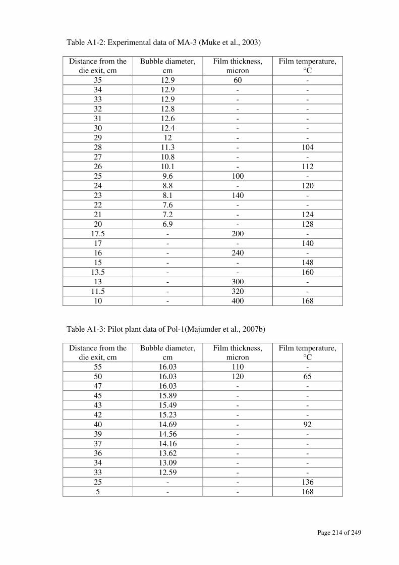
Page 214 of 249
Table A1-2: Experimental data of MA-3 (Muke et al., 2003)
Distance from the
die exit, cm
Bubble diameter,
cm
Film thickness,
micron
Film temperature,
°C
35 12.9 60 -
34 12.9 - -
33 12.9 - -
32 12.8 - -
31 12.6 - -
30 12.4 - -
29 12 - -
28 11.3 - 104
27 10.8 - -
26 10.1 - 112
25 9.6 100 -
24 8.8 - 120
23 8.1 140 -
22 7.6 - -
21 7.2 - 124
20 6.9 - 128
17.5 - 200 -
17 - - 140
16 - 240 -
15 - - 148
13.5 - - 160
13 - 300 -
11.5 - 320 -
10 - 400 168
Table A1-3: Pilot plant data of Pol-1(Majumder et al., 2007b)
Distance from the
die exit, cm
Bubble diameter,
cm
Film thickness,
micron
Film temperature,
°C
55 16.03 110 -
50 16.03 120 65
47 16.03 - -
45 15.89 - -
43 15.49 - -
42 15.23 - -
40 14.69 - 92
39 14.56 - -
37 14.16 - -
36 13.62 - -
34 13.09 - -
33 12.59 - -
25 - - 136
5 - - 168
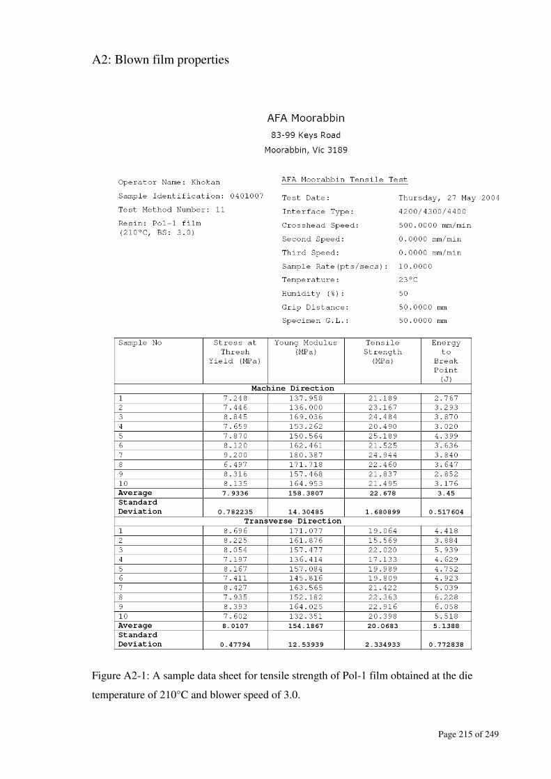
Page 215 of 249
A2: Blown film properties
Figure A2-1: A sample data sheet for tensile strength of Pol-1 film obtained at the die
temperature of 210°C and blower speed of 3.0.

Page 216 of 249
Table A2-1: Tensile strength (Average) of Pol-1 and Pol-2 film
Die
temperature,
°C
Blower
Speed
(BS)
Tensile
Strength of
Pol-1 in MD,
MPa
Tensile
Strength of
Pol-1 in TD,
MPa
Tensile
Strength of
Pol-2 in MD,
MPa
Tensile
Strength of
Pol-2 in TD,
MPa
200 3.0 22.32 20.76 16.26 15.01
200 2.8 21.77 19.07 16.97 14.66
200 2.6 21.61 20.03 17.28 16.96
200 2.4 22.59 19.38 16.31 17.25
210 3.0 22.68 20.07 16.55 14.25
210 2.8 23.37 21.90 16.15 14.68
210 2.6 22.88 21.37 15.99 15.52
210 2.4 22.46 22.05 14.88 13.25
220 3.0 22.86 21.17 15.19 13.67
220 2.8 21.92 20.19 14.80 15.76
220 2.6 21.76 20.45 14.26 13.57
220 2.4 20.61 23.03 13.37 12.14
Table A2-2: Tear strength (Average) of Pol-1 and Pol-2 film
Die
temperature,
°C
Blower
Speed
(BS)
Tear Strength
of Pol-1 in
MD, mN
Tear Strength
of Pol-1 in
TD, mN
Tear Strength
of Pol-2 in
MD, mN
Tear strength
of Pol-2 in
TD, mN
200 3.0 632 415 235 375
200 2.8 600 377 280 359
200 2.6 468 414 181 345
200 2.4 446 415 173 309
210 3.0 467 434 217 325
210 2.8 448 428 197 373
210 2.6 383 383 182 357
210 2.4 311 387 184 308
220 3.0 337 432 195 350
220 2.8 307 353 188 366
220 2.6 313 323 200 328
220 2.4 222 345 213 342
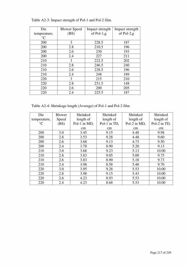
Page 217 of 249
Table A2-3: Impact strength of Pol-1 and Pol-2 film
Die
temperature,
°C
Blower Speed
(BS)
Impact strength
of Pol-1,g
Impact strength
of Pol-2,g
200 3 228.5 187
200 2.8 210.5 196
200 2.6 230 193
200 2.4 227 211
210 3 222.5 202
210 2.8 246.5 240
210 2.6 228.5 196
210 2.4 248 189
220 3 215 210
220 2.8 231.5 148
220 2.6 200 205
220 2.4 225.5 187
Table A2-4: Shrinkage length (Average) of Pol-1 and Pol-2 film
Die
temperature,
°C
Blower
Speed
(BS)
Shrinked
length of
Pol-1 in MD,
cm
Shrinked
length of
Pol-1 in TD,
cm
Shrinked
length of
Pol-2 in MD,
cm
Shrinked
length of
Pol-2 in TD,
cm
200 3.0 3.45 9.15 4.48 9.98
200 2.8 3.53 9.28 4.48 9.60
200 2.6 3.68 9.13 4.73 9.50
200 2.4 3.78 8.90 5.20 9.13
210 3.0 3.68 9.23 5.13 10.00
210 2.8 3.83 9.05 5.00 9.75
210 2.6 3.83 8.90 5.18 9.73
210 2.4 3.98 8.58 5.48 9.70
220 3.0 3.95 9.28 5.53 10.00
220 2.8 3.98 9.15 5.43 10.00
220 2.6 4.23 8.93 5.53 10.00
220 2.4 4.23 8.68 5.53 10.00
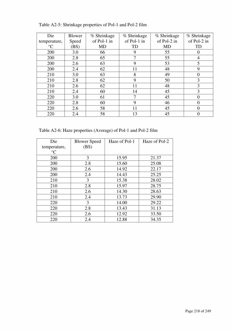
Page 218 of 249
Table A2-5: Shrinkage properties of Pol-1 and Pol-2 film
Die
temperature,
°C
Blower
Speed
(BS)
% Shrinkage
of Pol-1 in
MD
% Shrinkage
of Pol-1 in
TD
% Shrinkage
of Pol-2 in
MD
% Shrinkage
of Pol-2 in
TD
200 3.0 66 9 55 0
200 2.8 65 7 55 4
200 2.6 63 9 53 5
200 2.4 62 11 48 9
210 3.0 63 8 49 0
210 2.8 62 9 50 3
210 2.6 62 11 48 3
210 2.4 60 14 45 3
220 3.0 61 7 45 0
220 2.8 60 9 46 0
220 2.6 58 11 45 0
220 2.4 58 13 45 0
Table A2-6: Haze properties (Average) of Pol-1 and Pol-2 film
Die
temperature,
°C
Blower Speed
(BS)
Haze of Pol-1
Haze of Pol-2
200 3 15.95 21.37
200 2.8 15.60 25.08
200 2.6 14.92 22.17
200 2.4 14.43 25.25
210 3 15.38 28.02
210 2.8 15.97 28.75
210 2.6 14.30 28.63
210 2.4 13.73 29.90
220 3 14.00 29.22
220 2.8 13.43 31.13
220 2.6 12.92 33.50
220 2.4 12.88 34.35
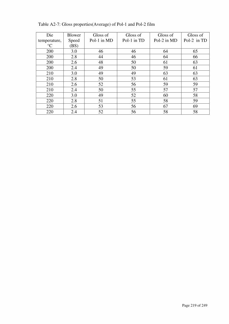
Page 219 of 249
Table A2-7: Gloss properties(Average) of Pol-1 and Pol-2 film
Die
temperature,
°C
Blower
Speed
(BS)
Gloss of
Pol-1 in MD
Gloss of
Pol-1 in TD
Gloss of
Pol-2 in MD
Gloss of
Pol-2 in TD
200 3.0 46 46 64 65
200 2.8 44 46 64 66
200 2.6 48 50 61 63
200 2.4 49 50 59 61
210 3.0 49 49 63 63
210 2.8 50 53 61 63
210 2.6 52 56 59 59
210 2.4 50 55 57 57
220 3.0 49 52 60 58
220 2.8 51 55 58 59
220 2.6 53 56 67 69
220 2.4 52 56 58 58
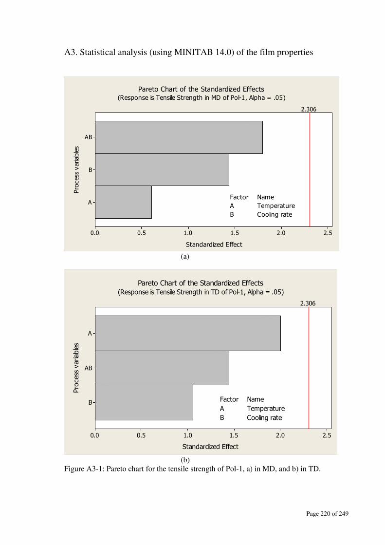
Page 220 of 249
A3. Statistical analysis (using MINITAB 14.0) of the film properties
Process variables
Standardized Effect
A
B
AB
2.52.01.51.00.50.0
2.306
Factor Name
A Temperature
B Cooling rate
Pareto Chart of the Standardized Effects
(Response is Tensile Strength in MD of Pol-1, Alpha = .05)
(a)
Process variables
Standardized Effect
B
AB
A
2.52.01.51.00.50.0
2.306
Factor Name
A Temperature
B Cooling rate
Pareto Chart of the Standardized Effects(Response is Tensile Strength in TD of Pol-1, Alpha = .05)
(b)
Figure A3-1: Pareto chart for the tensile strength of Pol-1, a) in MD, and b) in TD.
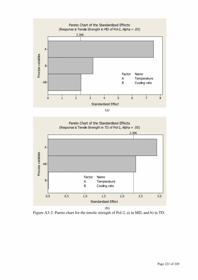
Page 221 of 249
Process variables
Standardized Effect
AB
B
A
876543210
2.306
Factor Name
A Temperature
B Cooling rate
Pareto Chart of the Standardized Effects(Response is Tensile Strength in MD of Pol-2, Alpha = .05)
(a)
Process variables
Standardized Effect
B
AB
A
3.02.52.01.51.00.50.0
2.306
Factor Name
A Temperature
B Cooling rate
Pareto Chart of the Standardized Effects(Response is Tensile Strength in TD of Pol-2, Alpha = .05)
(b)
Figure A3-2: Pareto chart for the tensile strength of Pol-2, a) in MD, and b) in TD.

Page 222 of 249
Process variables
Standardized Effect
AB
B
A
14121086420
2.31
Factor Name
A Temperature
B Cooling rate
Pareto Chart of the Standardized Effects(Response is Tear Strength in MD of Pol-1, Alpha = .05)
(a)
Process variables
Standardized Effect
AB
B
A
2.52.01.51.00.50.0
2.306
Factor Name
A Temperature
B Cooling rate
Pareto Chart of the Standardized Effects
(response is Tear Strength in TD of Pol-1, Alpha = .05)
(b)
Figure A3-3: Pareto chart for the tear strength of Pol-1, a) in MD, and b) in TD

Page 223 of 249
Process variables
Standardized Effect
A
B
AB
6543210
2.306
Factor Name
A Temperature
B Cooling rate
Pareto Chart of the Standardized Effects(Response is Tear strength in MD of Pol-2, Alpha = .05)
(a)
Process variables
Standardized Effect
A
AB
B
2.52.01.51.00.50.0
2.306
Factor Name
A Temperature
B Cooling rate
Pareto Chart of the Standardized Effects(Response is Tear Strength in TD of Pol-2, Alpha = .05)
(b)
Figure A3-4: Pareto chart for the tear strength of Pol-2, a) in MD, and b) in TD.

Page 224 of 249
Process variables
Standardized Effect
AB
A
B
2.52.01.51.00.50.0
2.306
Factor Name
A Temperature
B Cooling rate
Pareto Chart of the Standardized Effects
(Response is Impact strength of Pol-1, Alpha = .05)
Figure A3-5: Pareto chart of impact strength of Pol-1
Process variables
Standardized Effect
B
AB
A
2.52.01.51.00.50.0
2.306
Factor Name
A Temperature
B Cooling rate
Pareto Chart of the Standardized Effects(Response is Impact strength of Pol-2, Alpha = .05)
Figure A3-6: Pareto chart of impact strength of Pol-2

Page 225 of 249
Process variables
Standardized Effect
AB
B
A
14121086420
2.31
Factor Name
A Temperature
B Cooling rate
Pareto Chart of the Standardized Effects(response is Shrinkage in MD of Pol-1, Alpha = .05)
(a)
Process variables
Standardized Effect
A
AB
B
6543210
2.306
Factor Name
A Temperature
B Cooling rate
Pareto Chart of the Standardized Effects
(Response is Shrinkage in TD of Pol-1, Alpha = .05)
(b)
Figure A3-7: Pareto chart for the shrinkage properties of Pol-1, a) in MD, and b) in TD

Page 226 of 249
Process variables
Standardized Effect
AB
B
A
9876543210
2.306
Factor Name
A Temperature
B Cooling rate
Pareto Chart of the Standardized Effects(Response is Shrinkage in MD of Pol-2, Alpha = .05)
(a)
Process variables
Standardized Effect
AB
B
A
876543210
2.306
Factor Name
A Temperature
B Cooling rate
Pareto Chart of the Standardized Effects
(Response is Shrinkage in TD of Pol-2, Alpha = .05)
(b)
Figure A3-8: Pareto chart for the shrinkage properties of Pol-2, a) in MD, and b) in TD
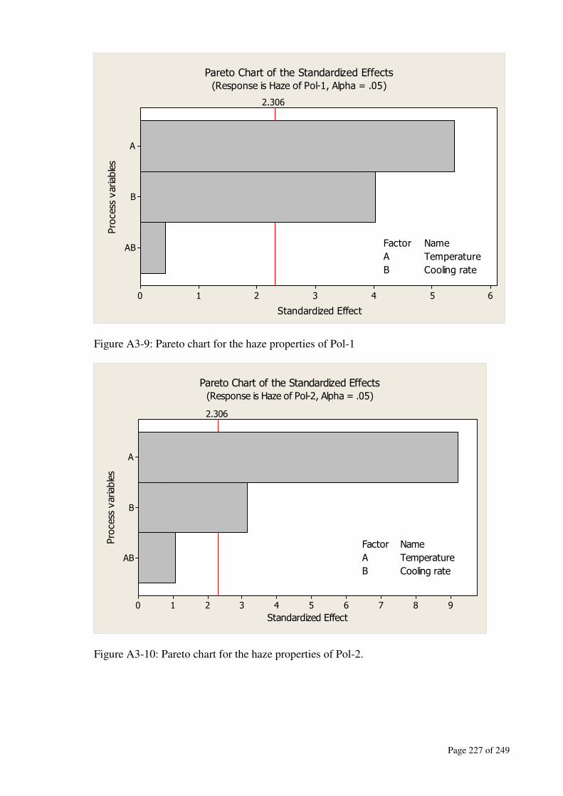
Page 227 of 249
Process variables
Standardized Effect
AB
B
A
6543210
2.306
Factor Name
A Temperature
B Cooling rate
Pareto Chart of the Standardized Effects(Response is Haze of Pol-1, Alpha = .05)
Figure A3-9: Pareto chart for the haze properties of Pol-1
Process variables
Standardized Effect
AB
B
A
9876543210
2.306
Factor Name
A Temperature
B Cooling rate
Pareto Chart of the Standardized Effects(Response is Haze of Pol-2, Alpha = .05)
Figure A3-10: Pareto chart for the haze properties of Pol-2.
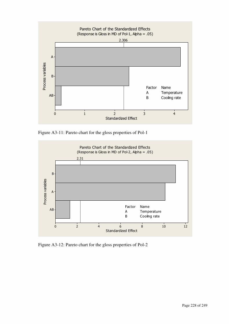
Page 228 of 249
Process variables
Standardized Effect
AB
B
A
43210
2.306
Factor Name
A Temperature
B Cooling rate
Pareto Chart of the Standardized Effects
(Response is Gloss in MD of Pol-1, Alpha = .05)
Figure A3-11: Pareto chart for the gloss properties of Pol-1
Process variables
Standardized Effect
AB
A
B
121086420
2.31
Factor Name
A Temperature
B Cooling rate
Pareto Chart of the Standardized Effects
(Response is Gloss in MD of Pol-2, Alpha = .05)
Figure A3-12: Pareto chart for the gloss properties of Pol-2

Page 229 of 249
(a)
(b)

Page 230 of 249
(c)
(d)
Figure A3-13: Normal probability plot of tensile strength properties: (a) Pol-1 in MD;
(b) Pol-1 in TD; (c) Pol-2 in MD; and (d) Pol-2 in TD
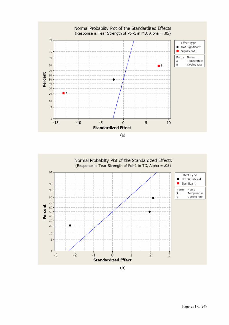
Page 231 of 249
(a)
(b)
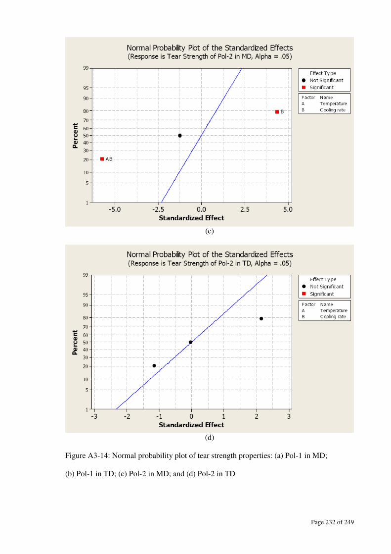
Page 232 of 249
(c)
(d)
Figure A3-14: Normal probability plot of tear strength properties: (a) Pol-1 in MD;
(b) Pol-1 in TD; (c) Pol-2 in MD; and (d) Pol-2 in TD
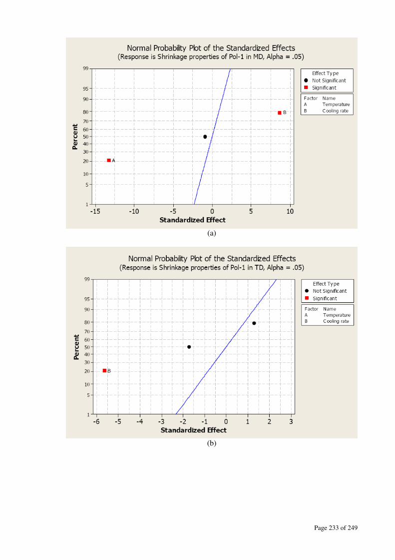
Page 233 of 249
(a)
(b)

Page 234 of 249
(c)
(d)
Figure A3-15: Normal probability plot of shrinkage properties: (a) Pol-1 in MD;
(b) Pol-1 in TD; (c) Pol-2 in MD; and (d) Pol-2 in TD
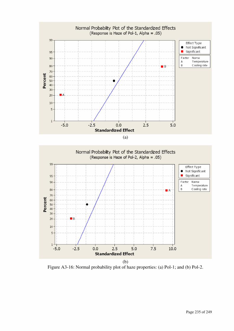
Page 235 of 249
(a)
(b)
Figure A3-16: Normal probability plot of haze properties: (a) Pol-1; and (b) Pol-2.

Page 236 of 249
(a)
(b)
Figure A3-17: Normal probability plot of gloss properties: (a) Pol-1 in MD; and
(b) Pol-2 in MD.
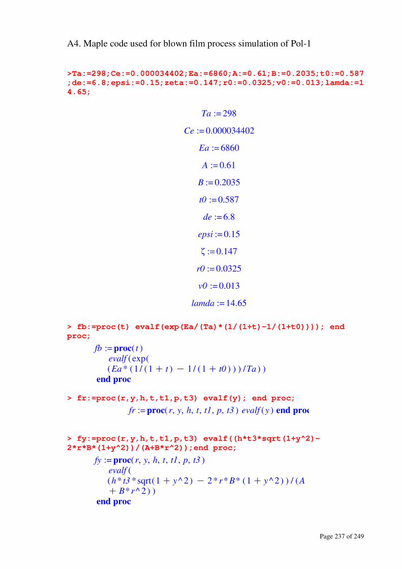
Page 237 of 249
A4. Maple code used for blown film process simulation of Pol-1
>Ta:=298;Ce:=0.000034402;Ea:=6860;A:=0.61;B:=0.2035;t0:=0.587
;de:=6.8;epsi:=0.15;zeta:=0.147;r0:=0.0325;v0:=0.013;lamda:=1
4.65;
Ta := 298
Ce := 0.000034402
Ea := 6860
A := 0.61
B := 0.2035
t0 := 0.587
de := 6.8
epsi := 0.15
z := 0.147
r0 := 0.0325
v0 := 0.013
lamda := 14.65
> fb:=proc(t) evalf(exp(Ea/(Ta)*(1/(1+t)-1/(1+t0)))); end
proc;
fb := proc( t )evalf (exp((Ea * (1 / (1 C t ) K 1 / (1 C t0 ) ) ) /Ta ) )
end proc
> fr:=proc(r,y,h,t,t1,p,t3) evalf(y); end proc;
fr := proc(r, y, h, t, t1, p, t3 ) evalf (y ) end proc
> fy:=proc(r,y,h,t,t1,p,t3) evalf((h*t3*sqrt(1+y^2)-
2*r*B*(1+y^2))/(A+B*r^2));end proc;
fy := proc(r, y, h, t, t1, p, t3 )evalf ((h* t3 *sqrt(1 C y^ 2 ) K 2 * r* B* (1 C y^ 2 ) ) / (A
C B* r^ 2 ) )end proc
Page 238 of 249
> fh:=proc(r,y,h,t,t1,p,t3) evalf((y/r*(t3/t1-1)-(1-
exp(epsi*de*(t1+t3+3*p)/fb(t))/de)+2*(1-
zeta)*r0*(1/(r*h))*y/r*(1+p/t1)/(sqrt(1+y^2))+2*ln(1/r*h^2)/(
(de^2)*t1))*h/(1-2*(1-zeta)*r0*(1/(r*h))/sqrt(1+y^2)-4*(1-
zeta)*1*p*(1/(r*h))/(t1*sqrt(1+y^2))));end proc;
fh := proc(r, y, h, t, t1, p, t3 )evalf
( ( ( (y* ( t3 / t1 K 1 ) ) /r K 1C exp( (epsi* de* ( t1 C t3 C 3 * p ) ) / fb ( t ) ) /de
C
(2* (1 K zeta) * r0* y* (1 C p / t1 ) ) / (r* h * r* sqrt(1C y^ 2 ) ) C (2 * ln(h ^ 2 /r ) ) / (de^ 2 * t1 ) ) * h )/ (1 K (2 * (1 K zeta) * r0 ) / (r* h *sqrt(1 C y^ 2 ) ) K (4* (1 K zeta) * p ) / (r* h * t1 * sqrt(1 C y^ 2 ) ) ) )
end proc
> fp:=proc(r,y,h,t,t1,p,t3) evalf(p/de*(1-
exp(epsi*de/fb(t)*(t1+t3+3*p)))+2(1-
zeta)*p*(1/(r*h))*fh(r,y,h,t,t1,p,t3)/(h*sqrt(1+y^2))-
2*ln(h)/de^2);end proc;
fp := proc(r, y, h, t, t1, p, t3 )evalf ((p* (1 K exp( (epsi* de* ( t1 C t3 C 3 * p ) ) / fb ( t ) ) ) ) /de
C
(2 (1 K zeta) * p* fh (r, y, h, t, t1, p, t3 ) ) / (r*h * h * sqrt(1C y^ 2 ) ) K (2 * ln(h ) ) /de^ 2 )
end proc
> ft11:=proc(r,y,h,t,t1,p,t3) evalf(t1/de*(1-
exp(epsi*de/fb(t)*(t1+t3+3*p)))-2*(1-
zeta)*(t1*(1/(r*h))*(fh(r,y,h,t,t1,p,t3)/h+y/r)/sqrt(1+y^2))-
2*(1-
zeta)*p*((1/(r*h))*(2*fh(r,y,h,t,t1,p,t3)/h+y/r)/sqrt(1+y^2))
-2*ln(1/r*h^2)/de^2);end proc;
ft11 := proc(r, y, h, t, t1, p, t3 )evalf (( t1 * (1 K exp( (epsi* de* ( t1 C t3 C 3 * p ) ) / fb ( t ) ) ) ) /de
K (2* (1 K zeta) * t1 * ( fh (r, y, h, t, t1, p, t3 ) /h
C y /r ) ) / (r* h * sqrt(1 C y^ 2) ) K (2 * (1 K zeta)* p * ( (2 * fh (r, y, h, t, t1, p, t3 ) ) /h C y /r ) ) / (r* h* sqrt(1C y^ 2 ) ) K (2 * ln(h ^ 2 /r ) ) /de^ 2 )
end proc
> ft33:=proc(r,y,h,t,t1,p,t3) evalf(t3/de*(1-
exp(epsi*de/fb(t)*(t1+t3+3*p)))+2*(1-
zeta)*(1/(r*h))/r*t3*y/sqrt(1+y^2)+2*(1-
zeta)*(1/(r*h))*p*(y/r-fh(r,y,h,t,t1,p,t3)/h)/sqrt(1+y^2)-
2*ln(r/h)/de^2);end proc;
Page 239 of 249
ft33 := proc(r, y, h, t, t1, p, t3 )evalf (( t3 * (1 K exp( (epsi* de* ( t1 C t3 C 3 * p ) ) / fb ( t ) ) ) ) /de
C (2 * (1 K zeta) * t3 * y ) / (r* h * r* sqrt(1 C y^ 2 ) )C
(2* (1 K zeta) * p* (y /r K fh (r, y, h, t, t1, p, t3 ) /h ) )/ (r* h *sqrt(1 C y^ 2 ) ) K (2 * ln(r /h ) ) /de^ 2 )
end proc
> fl:=proc(r,y,h,t,t1,p,t3)
evalf((A+B*r^2)*sqrt(1+y^2)/(r*h)); end proc;
fl := proc(r, y, h, t, t1, p, t3 )evalf ( ( (A C B* r^ 2 ) * sqrt(1 C y^ 2 ) ) / (r* h ) )
end proc
> ft:=proc(r,y,h,t,t1,p,t3)
evalf(Ce*(t3*y/r-t1*(fh(r,y,h,t,t1,p,t3)/h-y/r))-
2*22/7*(0.0325^2)*0.084*8.2*(560-780*exp(-1.27*(t*Ta)-
0.035*r))/(1+exp(x))*r*sqrt(1+y^2)*t/(2300*(7.5/3600))); end
proc;
ft := proc(r, y, h, t, t1, p, t3 )evalf (Ce * ( ( t3 * y ) /r
K t1 * ( fh (r, y, h, t, t1, p, t3 ) /h K y /r ) ) K 44 /7 * (0.0325^ 2 * 0.084* 8.2 * (560 K 780* exp(K1.27* t * Ta K 0.035 * r ) ) * r* sqrt(1C y^ 2 ) * t ) / ( (1 C exp(x ) ) * (2300* 7.5 ) /3600) )
end proc
> X:=45;n:=4500;dx:=evalf(X/n);
X := 45
n := 4500
dx := 0.01000000000
> solv:=proc(t0) local
kr1,kr2,kr3,kr4,ky1,ky2,ky3,ky4,kh1,kh2,kh3,kh4,kt1,kt2,kt3,k
t4,kft11,kft12,kft13,kft14,kft31,kft32,kft33,kft34,kp1,kp2,kp
3,kp4,k,hc;global
x,r,r1,y,h,h1,t,t1,t3,e11,e33,dx,n,f,g,fun,ft1,ft3,p,rpoints,
hpoints,tpoints,t1points,t3points,e11points,e33points,hcpoint
s;
Page 240 of 249
x:=0;r:=1; h:=1; y:=2.25; t:=t0;
t1:=1;t3:=0.1;p:=0;
rpoints:=[[x,r]];
hpoints:=[[x,h]];tpoints:=[[x,t]];t1points:=[[x,t1]];t3points
:=[[x,t3]];e11points:=[[x,e11]];e33points:=[[x,e33]];hcpoints
:=[[x,hc]];
for k from 1 to n while y>=0 do
x:=x+dx;
kr1:=fr(r,y,h,t,t1,p,t3);
ky1:=fy(r,y,h,t,t1,p,t3);
kh1:=fh(r,y,h,t,t1,p,t3);
kt1:=ft(r,y,h,t,t1,p,t3);
kft11:=ft11(r,y,h,t,t1,p,t3);
kft31:=ft33(r,y,h,t,t1,p,t3);
kp1:=fp(r,y,h,t,t1,p,t3);
kr2:=fr(r+dx*kr1/2,y+dx*ky1/2,h+dx*kh1/2,t+dx*kt1/2,t1+dx*kft
11/2,p+dx*kp1/2,t3+dx*kft31/2);
ky2:=fy(r+dx*kr1/2,y+dx*ky1/2,h+dx*kh1/2,t+dx*kt1/2,t1+dx*kft
11/2,p+dx*kp1/2,t3+dx*kft31/2);
kh2:=fh(r+dx*kr1/2,y+dx*ky1/2,h+dx*kh1/2,t+dx*kt1/2,t1+dx*kft
11/2,p+dx*kp1/2,t3+dx*kft31/2);
kt2:=ft(r+dx*kr1/2,y+dx*ky1/2,h+dx*kh1/2,t+dx*kt1/2,t1+dx*kft
11/2,p+dx*kp1/2,t3+dx*kft31/2);
kft12:=ft11(r+dx*kr1/2,y+dx*ky1/2,h+dx*kh1/2,t+dx*kt1/2,t1+dx
*kft11/2,p+dx*kp1/2,t3+dx*kft31/2);
kft32:=ft33(r+dx*kr1/2,y+dx*ky1/2,h+dx*kh1/2,t+dx*kt1/2,t1+dx
*kft11/2,p+dx*kp1/2,t3+dx*kft31/2);
kp2:=fp(r+dx*kr1/2,y+dx*ky1/2,h+dx*kh1/2,t+dx*kt1/2,t1+dx*kft
11/2,p+dx*kp1/2,t3+dx*kft31/2);
kr3:=fr(r+dx*kr2/2,y+dx*ky2/2,h+dx*kh2/2,t+dx*kt2/2,t1+dx*kft
12/2,p+dx*kp2/2,t3+dx*kft32/2);
ky3:=fy(r+dx*kr2/2,y+dx*ky2/2,h+dx*kh2/2,t+dx*kt2/2,t1+dx*kft
12/2,p+dx*kp2/2,t3+dx*kft32/2);
kh3:=fh(r+dx*kr2/2,y+dx*ky2/2,h+dx*kh2/2,t+dx*kt2/2,t1+dx*kft
12/2,p+dx*kp2/2,t3+dx*kft32/2);
kt3:=ft(r+dx*kr2/2,y+dx*ky2/2,h+dx*kh2/2,t+dx*kt2/2,t1+dx*kft
12/2,p+dx*kp2/2,t3+dx*kft32/2);
kft13:=ft11(r+dx*kr2/2,y+dx*ky2/2,h+dx*kh2/2,t+dx*kt2/2,t1+dx
*kft12/2,p+dx*kp2/2,t3+dx*kft32/2);
kft33:=ft33(r+dx*kr2/2,y+dx*ky2/2,h+dx*kh2/2,t+dx*kt2/2,t1+dx
*kft12/2,p+dx*kp2/2,t3+dx*kft32/2);
kp3:=fp(r+dx*kr2/2,y+dx*ky2/2,h+dx*kh2/2,t+dx*kt2/2,t1+dx*kft
12/2,p+dx*kp2/2,t3+dx*kft32/2);
kr4:=fr(r+dx*kr3,y+dx*ky3,h+dx*kh3,t+dx*kt3,t1+dx*kft13,p+dx*
kp3,t3+dx*kft33);
ky4:=fy(r+dx*kr3,y+dx*ky3,h+dx*kh3,t+dx*kt3,t1+dx*kft13,p+dx*
kp3,t3+dx*kft33);
kh4:=fh(r+dx*kr3,y+dx*ky3,h+dx*kh3,t+dx*kt3,t1+dx*kft13,p+dx*
kp3,t3+dx*kft33);

Page 241 of 249
kt4:=ft(r+dx*kr3,y+dx*ky3,h+dx*kh3,t+dx*kt3,t1+dx*kft13,p+dx*
kp3,t3+dx*kft33);
kft14:=ft11(r+dx*kr3,y+dx*ky3,h+dx*kh3,t+dx*kt3,t1+dx*kft13,p
+dx*kp3,t3+dx*kft33);
kft34:=ft33(r+dx*kr3,y+dx*ky3,h+dx*kh3,t+dx*kt3,t1+dx*kft13,p
+dx*kp3,t3+dx*kft33);
kp4:=fp(r+dx*kr3,y+dx*ky3,h+dx*kh3,t+dx*kt3,t1+dx*kft13,p+dx*
kp3,t3+dx*kft33);
r:=r+1/6*(kr1+2*kr2+2*kr3+kr4)*dx;
y:=y+1/6*(ky1+2*ky2+2*ky3+ky4)*dx;
h:=h+1/6*(kh1+2*kh2+2*kh3+kh4)*dx;
t:=t+1/6*(kt1+2*kt2+2*kt3+kt4)*dx;
t1:=t1+1/6*(kft11+2*kft12+2*kft13+kft14)*dx;
t3:=t3+1/6*(kft31+2*kft32+2*kft33+kft34)*dx;
p:=p+1/6*(kp1+2*kp2+2*kp3+kp4)*dx;
e11:=1/(r*h)*1/(sqrt(1+y^2))*(-(1/h)*fh(r,y,h,t,t1,p,t3)-
(1/r)*y);
e33:=1/(r*h)*1/(sqrt(1+y^2))*y/r;
hc:=0.084*3.5*(560-780*exp(-1.27*(t*Ta)-0.035*r))/(1+exp(x));
rpoints:=[op(rpoints),[x,r]];
hpoints:=[op(hpoints),[x,h]];
tpoints:=[op(tpoints),[x,t]];
t1points:=[op(t1points),[x,t1]];
t3points:=[op(t3points),[x,t3]];
e11points:=[op(e11points),[x,e11]];
e33points:=[op(e33points),[x,e33]];
hcpoints:=[op(hcpoints),[x,hc]];
od:
end proc;
>solv(0.587);
> plot(rpoints,labels=["distance","diameter"]);

Page 242 of 249
> plot(hpoints,labels=["distance","thickness"]);
> plot(tpoints,labels=["distance","temp"]);
> plot(t1points,labels=["distance","Stress in MD"]);
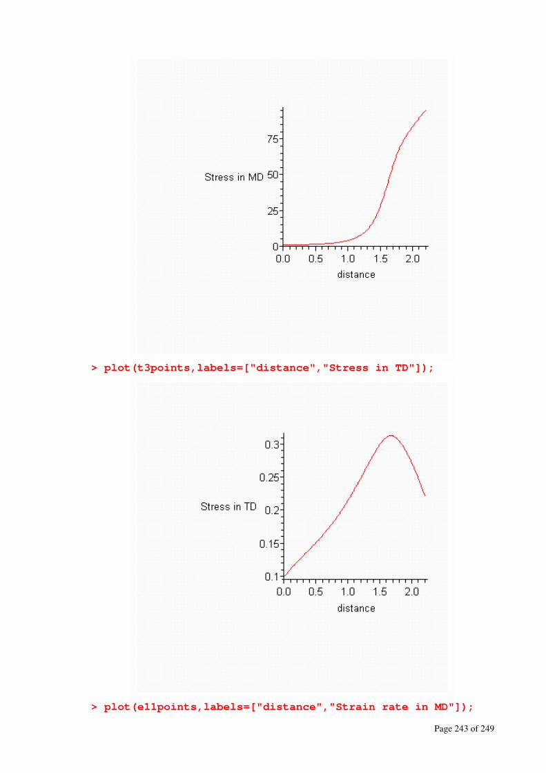
Page 243 of 249
> plot(t3points,labels=["distance","Stress in TD"]);
> plot(e11points,labels=["distance","Strain rate in MD"]);
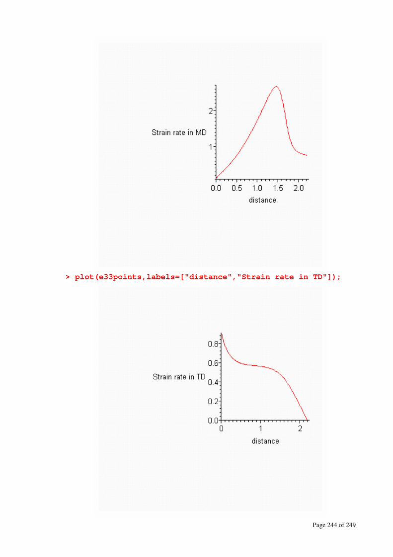
Page 244 of 249
> plot(e33points,labels=["distance","Strain rate in TD"]);

Page 245 of 249
> plot(hcpoints,labels=["distance","HTC,w/m^2/k"]);

Page 246 of 249
List of Symbols used for blown film modelling and simulation
Nomenclatures
aT Shift factor
A Dimensionless tensile force
B Dimensionless bubble pressure
BUR Blow up ratio
C Dimensionless stress in the transverse direction
Ce Dimensionless energy dissipation coefficinet
Ch Dimensionless heat transfer coefficient
Cp Specific heat of the polymer
De Deborah number
Ea Flow activation enrgy
Fz Tensile force at the freeze line
FLH Freeze line height
gi Relaxation modulus of the i-th component
G0 Zero shear elastic modulus
G' Elastic modulus
h Dimensionless film thickness
H Local film thickness
Hc Heat transfer coefficient
L Dimensionless tress in the machine direction
LFW Lay flat width of the film
mɺ Mass flow rate
p Isotropic pressure
∆P Pressure variation
Q Volumetric flow rate
r Dimensionless bubble radius
R Local Bubble radius
R1 Radii of curvature in the machine direction
R3 Radii of curvature in the transverse direction
t Dimensionless temperature
T Temperature
Ta Ambient air temperature
Tc Crystallization temperature of the polymer
V Linear velocity
v Dimensionless velocity
vm Velocity in the machine direction
vt Velocity in the transverse direction
vn Velocity in the normal direction
z Dimensionless distance in the axial direction
ZFL Distance between the die exit and freeze line
Greek Letters
δ Kronecker delta ε Extensional property in the PTT model
ijε Deformation tensor
ijεɺ Deformation rate tensor
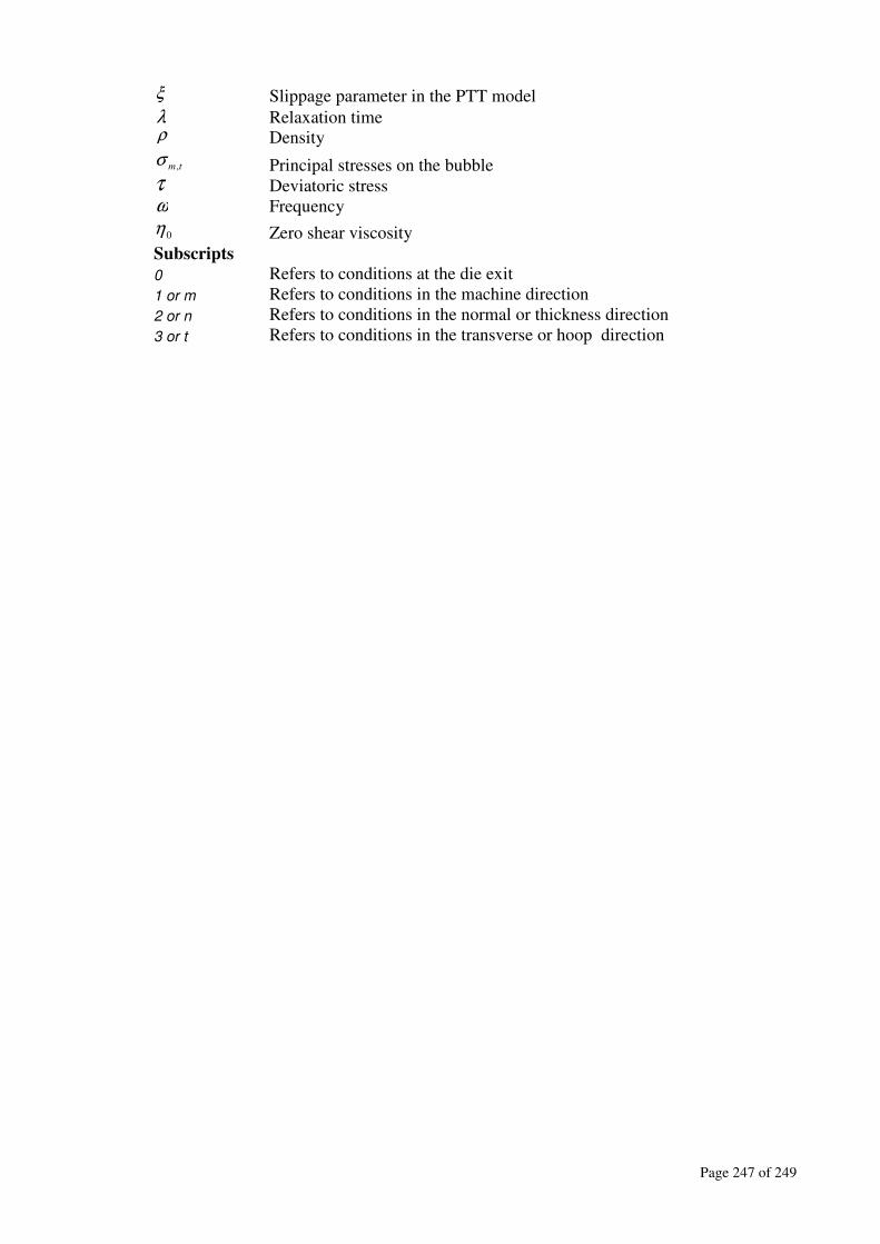
Page 247 of 249
ξ Slippage parameter in the PTT model
λ Relaxation time ρ Density
tm,σ Principal stresses on the bubble τ Deviatoric stress ω Frequency
0η Zero shear viscosity
Subscripts
0 Refers to conditions at the die exit
1 or m Refers to conditions in the machine direction
2 or n Refers to conditions in the normal or thickness direction
3 or t Refers to conditions in the transverse or hoop direction
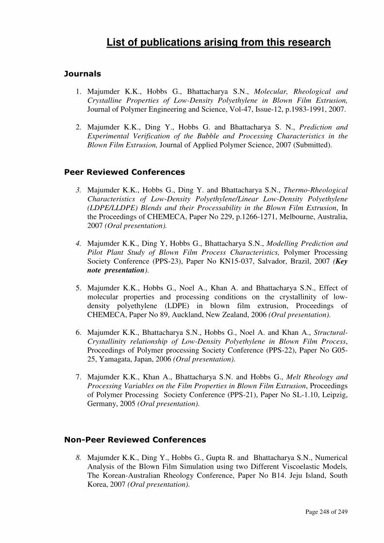
Page 248 of 249
List of publications arising from this research
Journals
1. Majumder K.K., Hobbs G., Bhattacharya S.N., Molecular, Rheological and
Crystalline Properties of Low-Density Polyethylene in Blown Film Extrusion,
Journal of Polymer Engineering and Science, Vol-47, Issue-12, p.1983-1991, 2007.
2. Majumder K.K., Ding Y., Hobbs G. and Bhattacharya S. N., Prediction and
Experimental Verification of the Bubble and Processing Characteristics in the
Blown Film Extrusion, Journal of Applied Polymer Science, 2007 (Submitted).
Peer Reviewed Conferences
3. Majumder K.K., Hobbs G., Ding Y. and Bhattacharya S.N., Thermo-Rheological
Characteristics of Low-Density Polyethylene/Linear Low-Density Polyethylene
(LDPE/LLDPE) Blends and their Processability in the Blown Film Extrusion, In
the Proceedings of CHEMECA, Paper No 229, p.1266-1271, Melbourne, Australia,
2007 (Oral presentation).
4. Majumder K.K., Ding Y, Hobbs G., Bhattacharya S.N., Modelling Prediction and
Pilot Plant Study of Blown Film Process Characteristics, Polymer Processing
Society Conference (PPS-23), Paper No KN15-037, Salvador, Brazil, 2007 (Key
note presentation).
5. Majumder K.K., Hobbs G., Noel A., Khan A. and Bhattacharya S.N., Effect of
molecular properties and processing conditions on the crystallinity of low-
density polyethylene (LDPE) in blown film extrusion, Proceedings of
CHEMECA, Paper No 89, Auckland, New Zealand, 2006 (Oral presentation).
6. Majumder K.K., Bhattacharya S.N., Hobbs G., Noel A. and Khan A., Structural-
Crystallinity relationship of Low-Density Polyethylene in Blown Film Process,
Proceedings of Polymer processing Society Conference (PPS-22), Paper No G05-
25, Yamagata, Japan, 2006 (Oral presentation).
7. Majumder K.K., Khan A., Bhattacharya S.N. and Hobbs G., Melt Rheology and
Processing Variables on the Film Properties in Blown Film Extrusion, Proceedings
of Polymer Processing Society Conference (PPS-21), Paper No SL-1.10, Leipzig,
Germany, 2005 (Oral presentation).
Non-Peer Reviewed Conferences
8. Majumder K.K., Ding Y., Hobbs G., Gupta R. and Bhattacharya S.N., Numerical
Analysis of the Blown Film Simulation using two Different Viscoelastic Models,
The Korean-Australian Rheology Conference, Paper No B14. Jeju Island, South
Korea, 2007 (Oral presentation).

Page 249 of 249
9. Majumder K.K., Bhattacharya S.N., Hobbs G., Khan A., McLean C. and Noel A.,
Effect of the Cooling Rate and the Relaxation Properties of LDPE Melt on the Film
Properties in the Blown Film Extrusion, Proceedings of Australian-
Korean Rheology Conference(AKRC), Paper No F16, Cairns, Australia, 2005
(Oral presentation).
Journal Paper Ready to Submit
10. Majumder K.K., Hobbs G., Ding Y and Bhattacharya S. N, Effect of Long Chain
Branching (LCB) on the melt rheology and blown film properties of Low-Density
Polyethylene (LDPE), Polymer International, 2007.


