
Black Bass Habitat Use and Availability at Multiple Scales in Middle Chattahoochee River
Tributaries
by
Charles Theophilos Katechis
A thesis submitted to the Graduate Faculty of
Auburn University
in partial fulfillment of the
requirements for the Degree of
Fisheries, Master of Science
Auburn, Alabama
December 12, 2015
Keywords: black bass, stream habitat, land use, stream survey,
side-scan sonar, distribution
Copyright 2015 by Charles Theophilos Katechis
Approved by
Terrill R. Hanson, Chair, Professor, School of Fisheries, Aquaculture, and Aquatic Science
Steven Sammons, Research Fellow IV, School of Fisheries, Aquaculture, and Aquatic Science
Jim Stoeckel, Associate Professor, School of Fisheries, Aquaculture, and Aquatic Science

ii
Abstract
The focus of this study was on tributaries of the Middle Chattahoochee River where
Shoal Bass Micropterus cataractae and Chattahoochee Bass Micropterus chattahoochae are
experiencing declines, mainly due to anthropogenic disturbances of streams and introductions of
non-native congeners. This study examined habitat use of black bass and the presence/absence of
Shoal Bass and Chattahoochee Bass at multiple scales. Point and transect surveys, canoe surveys,
side-scan sonar mapping techniques, and available land use data were used to measure habitat
characteristics at each scale. Black bass were sampled by both backpack electrofishing and by
canoe-mounted electrofishing. Results indicated that suitable habitat for Shoal Bass included
rocky boulder habitats with shallow depths and wide stream banks in heavily forested areas of
large watersheds and Chattahoochee Bass were found in highly natural and forested land cover
areas small watersheds in wider sections of the stream in rocky and shallow fast-moving shoal
habitats. Surveys revealed that Shoal Bass populations can persist in smaller watersheds with
enough ideal habitat. Chattahoochee Bass would likely benefit from habitat restoration for Shoal
Bass in streams where they are sympatric. Side-scan sonar surveys were conducted on smaller
streams, smaller than previously attempted, and results indicated that this method was useful to
map habitat in these systems. Conclusions of this study indicated that priority streams for Shoal
Bass and/or Chattahoochee Bass restoration, restocking efforts, and the reduction in non-native
bass populations included the Dog River, Centralhatchee, Hillabahatchee, Wehadkee, Mountain
Oak, and Osanippa creeks.

iii
Acknowledgments
I thank my mother, Angia A. Katechis, and my family for their continued support in
pursuit of my graduate degree. I also thank the Thompson family for the help they provided
during and after my undergraduate years. I thank Dr. Steven M. Sammons for hiring me as a
field technician and then taking me on as a graduate student. He gave me an opportunity to
continue my career in fisheries biology and has helped me throughout my graduate research. I
thank Dr. Terry Hanson for giving me the opportunity to pursue a master's degree and his
commitment, support, and guidance throughout the project. Also Dr. Jim Stoeckel has given me
great insight on what my research objectives should focus on. I am very thankful for the
assistance I have received from Kat Hoenke of the Southeast Aquatic Resource Partnership
(SARP) who provided me with needed land use data.
This study was funded by the Georgia Power Company (GPC), National Fish and
Wildlife Foundation (NFWF), Georgia Department of Natural Resource - Wildlife Resource
Division, Fisheries Management and Non-game Conservation sections (GADNR-WRD). I thank
Joey Slaughter, GPC, for use of an extra backpack electrofisher. I thank Thom Litts, a GIS
specialist for the GADNR-WRD, for use of side-scan sonar equipment, and providing guidance
on the interpretation and acquisition of instream habitat data. I thank Auburn University
personnel including Scott Snyder for their help on many project tasks. Finally, I thank David
Belkoski, a field technician, and the many members of my field crew including undergraduate
and graduate students.

iv
Table of Contents
Abstract ........................................................................................................................................... ii
Acknowledgments.......................................................................................................................... iii
List of Tables ................................................................................................................................. vi
List of Figures ............................................................................................................................... vii
List of Abbreviations .................................................................................................................. viii
Definitions of Note ....................................................................................................................... ix
I. Introduction .................................................................................................................................1
I.1. Black Bass in the Chattahoochee River Basin...............................................................1
I.2. Black Bass Business Plan and Habitat Importance ......................................................3
I.3. Habitat Surveys .............................................................................................................4
I.4. Research Goals .............................................................................................................8
II. Methods ......................................................................................................................................9
II.1. Study Area ...................................................................................................................9
II.2. Field Surveys .............................................................................................................10
II.2.1. Microhabitat Survey ...................................................................................10
II.2.2. Mesohabitat Survey and Side-Scan Sonar Survey ......................................11
II.3. Macrohabitat Survey and Overall Habitat Analyses ..................................................13
III. Results .....................................................................................................................................17
III.1. Microhabitat Scale ....................................................................................................17

v
III.2. Mesohabitat Scale ....................................................................................................20
III.3. Macrohabitat Scale ...................................................................................................22
III.4. Side-Scan Sonar Analysis .........................................................................................25
V. Discussion ................................................................................................................................27
V.1. Connectivity and Stream Habitat Restoration ............................................................28
V.2. Land Use Conclusions ...............................................................................................30
V.3. Congeneric Spotted Bass Invasion .............................................................................32
V.4. Side-Scan Sonar Surveys of Small Streams ...............................................................33
V.5. Future Analyses..........................................................................................................35
VI. Conclusions and Management Implications ............................................................................36
VII. Literature Cited .....................................................................................................................42
VIII. Tables ..................................................................................................................................48
IX. Figures ...................................................................................................................................67
X. Appendices ..............................................................................................................................81
X.1. Side-Scan Sonar Start and End GPS Points ...............................................................82
X.2. Point and Transect Habitat Sampling Form .............................................................83
X.3. Point and Transect Electrofishing Form ....................................................................84
X.4. Handheld Canoe Electrofishing Transect Form .........................................................85
X.5. Land Cover Classifications ........................................................................................86

vi
List of Tables
Table 1. Stream Sampling Locations ...........................................................................................49
Table 2. Modified Wentworth Scale of Substrates .......................................................................50
Table 3. Catch and Effort of Point and Transect Surveys.............................................................51
Table 4. Percent Substrate and Percent Cover of Point and Transect Surveys .............................52
Table 5. Pearson’s R Correlations of Microhabitats .....................................................................53
Table 6. Pearson’s R Correlations of Black Bass to Microhabitats ..............................................54
Table 7. Shoal Bass Microhabitat Predictive Model ....................................................................55
Table 8. Spotted Bass Microhabitat Predictive Model .................................................................56
Table 9. Largemouth Bass Microhabitat Predictive Model ..........................................................57
Table 10. Chattahoochee Bass Microhabitat Predictive Model ....................................................58
Table 11. Catch, Effort, and Mean Mesohabitats of Canoe Handheld Electrofishing Surveys ....59
Table 12. Pearson’s R Correlations of Black Bass to Mesohabitat .............................................60
Table 13. Black Bass Mesohabitat Predictive Model ...................................................................61
Table 14. Middle Chattahoochee River Watershed Land Cover Area Totals ..............................62
Table 15. Shoal Bass and Chattahoochee Bass Watershed Land Cover Area Comparisons ........63
Table 16. Shoal Bass and Chattahoochee Bass Watershed Percent Land Cover Comparisons ...64
Table 17. Side-Scan Sonar Stream Substrate Totals .....................................................................65
Table 18. Side-Scan Sonar Stream Substrate Percentages............................................................66

vii
List of Figures
Figure 1. Map of Middle Chattahoochee River Tributaries ..........................................................68
Figure 2. Example Raw Side-Scan Sonar Image and Sonar Image with Collar Removed ..........69
Figure 3. Example Side-Scan Sonar Image of a Generated Control Point Network, Rectified
Stream Imagery, and Habitat Delineation of Imagery .......................................................70
Figure 4. Percent of Substrate in each Mesohabitat for Point and Transect Surveys ...................71
Figure 5. Shoal Bass and Chattahoochee Bass Presence/Absence Stream Velocity
Comparisons ......................................................................................................................72
Figure 6. Shoal Bass and Chattahoochee Bass Presence/Absence Stream Depth Comparisons ..73
Figure 7. Shoal Bass and Chattahoochee Bass Presence/Absence Stream Width Comparisons ..74
Figure 8. Shoal Bass and Chattahoochee Bass Presence/Absence Mean Substrate
Comparisons ......................................................................................................................75
Figure 9. Shoal Bass and Chattahoochee Bass Presence/Absence Mean Mesohabitat
Comparisons ......................................................................................................................76
Figure 10. Side-Scan Sonar and Point Transect Overall Comparisons of Substrate for Flat Shoals
and Mulberry Creeks..........................................................................................................77
Figure 11. Side-Scan Sonar and Point Transect Overall Comparisons of Substrate for Mountain
Oak and Halawakee Creeks ...............................................................................................78
Figure 12. Side-Scan Sonar and Point Transect Overall Comparisons of Substrate for Osanippa
Creek ..................................................................................................................................79
Figure 13. Side-Scan Sonar and Point Transect Overall Comparisons of Substrate for All
Mapped Streams.................................................................................................................80

viii
List of Abbreviations
ALDWFF Alabama Division of Wildlife and Freshwater Fisheries
BD Bedrock
BR Boulder
COB Cobble
CPE Catch-per-effort
GADNR Georgia Department of Natural Resources
GLM Generalized Linear Model
GPC Georgia Power Company
GR Gravel
MMU Minimum Mapping Unit
MSW Mean stream width
NFWF National Fish and Wildlife Foundation
NLCD National Land Cover Database
NBBI Native Black Bass Keystone Initiative
RRET Representative Reach Extrapolation Technique
SARP Southeast Aquatic Resource Partnership
SD Sand
WRD Wildlife Resources Division
USGS United States Geological Survey

ix
Definitions of Note
Mesohabitat An intermediate scale of habitat in streams defined by laminar or turbulent
flow, depth, and substrate particle size. Examples include: pools, riffles,
runs, and shoals.
Microhabitat A small scale measure of physical conditions in a localized area of a
stream. Examples include: depth, fluid velocity, stream width, and
substrate particle size.
Pool A type of stream mesohabitat defined by slow-moving laminar flow,
moderate to deep depth, and typically consists of sand and silt substrates.
Reach A section of stream defined arbitrarily or based on geology, stream access,
or area of concern that typically consists of multiple stream mesohabitats.
Riffle A type of stream mesohabitat defined by moderate turbulent flows,
shallow depths and typically smaller diameter substrates.
Run A type of stream mesohabitat defined by relatively laminar flow, moderate
to shallow depth, and typically lack rocky substrates.
Shoal A type of stream mesohabitat defined by highly turbulent flow and rapids,
eddie currents, shallow to moderate depth, and rocky substrates.
Side-Scan Sonar Use of a boat-mounted sonar device that emits a pulse towards the stream
bottom and sends back an acoustic image that allows the viewer to
interpret habitat from the stream floor based on shape, intensity, and
pattern of images.

1
I. INTRODUCTION
Types of anthropogenic disturbances affecting native communities of aquatic organisms
include biological introduction of non-native species, river impoundments by dams,
channelization of rivers, bank erosion caused by changes in land use, water withdrawal, and
nutrient point-source pollution caused by farming and urban practices (Webster et al. 1992;
Doyle et al. 2005; Simon and Rinaldi 2006). Shoal Bass Micropterus cataractae are a native
black bass that is experiencing declines through their native range. Once prolific throughout the
Chattahoochee River, Alabama-Georgia, construction of numerous dams resulted in widespread
declines in Shoal Bass populations. Currently, Shoal Bass in the Chattahoochee Basin south of
Atlanta, Georgia, persist in small isolated populations below dams in the main channel and in
tributaries streams (Boschung and Mayden 2004; Stormer and Maceina 2008; Sammons and
Maceina 2009). This study focused on populations of black bass in tributary streams of the
Middle Chattahoochee River and their habitat use and habitat availability.
I.1. Black Bass in the Chattahoochee River Basin
Shoal Bass are endemic to the Apalachicola River drainage, which includes the
Apalachicola, Chattahoochee, and Flint rivers in portions of Alabama, Georgia, and Florida.
Additionally, the species was introduced in the 1970s into the Ocmulgee River, Georgia, a major
river in the Altamaha River Basin (Sammons et al. 2015). The holotype for the Shoal Bass was
collected in the upper Chipola River, Florida, a tributary of the Apalachicola River (Williams
and Burgess 1999). Shoal Bass are considered to be fluvial specialists that prefer rocky riffles,
shoals, and runs, are typically found in small to medium rivers and streams, and are intolerant to
lentic conditions (Williams and Burgess 1999).

2
In 1989 Shoal Bass were assigned a status of Special Concern by the American Fisheries
Society Endangered Species Committee (Williams et. al 1989). In Alabama, Shoal Bass were
historically found in Osanippa, Halawakee, Little Uchee, Wacoochee, and Wehadkee creeks
(Williams and Burgess 1999; Boschung and Mayden 2004), but surveys in the mid-2000s
revealed that Shoal Bass had been nearly extirpated from three of these streams (Stormer and
Maceina 2008). In 2004 the species was assigned a status of High Conservation Concern in
Alabama (Mirarchi et al. 2004), their harvest was consequently prohibited on October 1, 2006,
and in 2007 the Alabama Division of Wildlife and Freshwater Fisheries (ALDWFF) initiated a
restocking program in an attempt to restore populations in these tributaries. However, follow-up
surveys conducted to determine the success of restocking found few stocked Shoal Bass
(Sammons and Maceina 2009). Severe droughts before, during, and after restocking may have
influenced the success of the stocking effort by reducing abundance in prey species and
increasing the potential for competition by native and introduced congeneric species (Stormer
and Maceina 2008).
The Chattahoochee Bass M. chattahoochae is a black bass that was recently described by
Baker et al. (2013) as being endemic to the Chattahoochee River and as member of the Redeye
Bass M. coosae species group. It differs from all other members by having broad margins of
bright orange pigment on posterior dorsal, caudal, and anal fins and by a wider head than other
species within the group. The holotype for Chattahoochee Bass was collected in Centralhatchee
Creek in March 2009, and they have since been collected during this study in Whooping Creek,
Snake Creek, and Dog River within the Middle Chattahoochee River.
The Spotted Bass M. punctulatus was introduced into the Apalachicola River Basin
below the Fall Line in the Flint River sometime prior to 1941, near the present day location of

3
Lake Seminole (Williams and Burgess 1999). A second introduction of Spotted Bass in the
1960s occurred above the Fall Line in the Chattahoochee River upstream of hydropower dams
near Columbus, Georgia. Additional collections of Alabama Bass M. henshalli occurred in the
1970s on the upper Chattahoochee River above Atlanta, Georgia (Williams and Burgess 1999).
The threat of introgressive hybridization is a well-documented, serious concern for the genetic
integrity of native black bass populations that could lead to major shifts in the specialization of
well-adapted endemic fish species (Koppelman 1994; Avise et al.1997; Barwick et al. 2006).
Morizot et al. (1991) documented the loss of genetic integrity of native Guadalupe Bass M.
treculi through multispecies hybridizations with introduced Smallmouth Bass M. dolomieu and
Florida Largemouth Bass M. salmoides floridanus. However, the effects of introduced Spotted
Bass on native Shoal Bass have been little studied. Habitat partitioning occurs naturally between
native Shoal Bass and Largemouth Bass M. salmoides (Wheeler and Allen 2003); but,
Goclowski et al. (2013) found that the introduced Spotted Bass in Flint River, Georgia,
functioned as an intermediate habitat generalist, suggesting that Spotted Bass could serve as a
competitor for resources for either native species. Spotted Bass are highly adaptable, able to
persist equally well in reservoirs and small streams (Churchill and Bettoli 2015); whereas Shoal
Bass populations have been fragmented into relatively discrete populations between reservoirs
because of their intolerance to lentic conditions (Wheeler and Allen 2003; Boschung and
Mayden 2004; Stormer and Maceina 2008).
I.2. Black Bass Business Plan and Habitat Importance
The National Fish and Wildlife Foundation (NFWF) Native Black Bass Keystone
Initiative (NBBI) selected the Middle Chattahoochee River as an area of focus for conserving
native endemic black bass species in the southeastern United States (Birdsong et al. 2010; Figure
4
1). Efforts to protect charismatic species, like Shoal Bass and Chattahoochee Bass, in aquatic
environments may also help in protecting other sympatric species such as other fishes, mussels,
plants, and crayfish. Shoal habitats appear to be important for the persistence of these native
black bass in tributaries of the Middle Chattahoochee River and Shoal Bass were documented
traveling up tributary streams via radio telemetry, presumably to spawn (Sammons and Earley
2015). Georgia Power Company biologists have also collected large numbers of age-0 Shoal
Bass in large shoals within Chattahoochee River tributaries (J. Slaughter, Georgia Power
Company, unpublished data). Larval, juvenile, and adult Shoal Bass have also been shown to
express ontogenetic shifts in the use of distinct microhabitats (boulder substrates at varying
depth) within shoals (Johnston and Kennon 2007), so differing microhabitat availability may be
important for future restoration efforts.
There have been numerous studies documenting the effects of habitat alteration on the
imperilment of freshwater fishes e.g., (Warren et al. 2000; Sullivan et al. 2004; Diana, Allan, and
Infante 2006; Hrodey 2009), and Middle Chattahoochee River tributaries are suffering similar
habitat loss from increased sedimentation (siltation and impacted rocky substrate) and altered
hydrology from changing land use (Walser and Bart 1999). Determining habitat suitability can
assist biologists in finding optimum habitat for fish species, including velocity, depth, substrate,
and cover use (Freeman et al. 1997).
I.2. Habitat Surveys
A widely-used method for measuring habitat is the representative reach extrapolation
technique (RRET), where biologists measure habitat in a particular reach of stream and
extrapolate those metrics to larger scales. Reaches selected in the RRET are assumed to yield
habitat estimates that are representative of the entire stream or watershed, and the location,

5
length, and number of reaches can vary depending on the expected heterogeneity of the stream
habitat (Doloff and Jennings 1997). The RRET assists in identifying discrete hydraulic channel
units, provides quantitative descriptions of each channel unit, and identifies statistical differences
in microhabitat characteristics. Stream reaches are typically sampled by some form of point and
transect surveys which are a standardized method for collecting data specific to a reach that
represents a stream (Simonson 1994; Perkin 2010; Fore et al. 2011). Data collected included
metrics of microhabitat, and black bass species catch data within multiple mesohabitats. Data
collected informs conditions of microhabitat and catch of black bass species within specific
mesohabitats (Sammons and Maceina 2009). Until recently, use of methods like the RRET were
difficult in larger, non-wadeable streams due to the logistics and manpower required to quantify
habitat in these streams. Kaeser and Litts (2010) developed a side-scan sonar technique for
mapping continuous instream habitat across broad aquatic basins. Side-scan sonar is typically
used for mapping larger streams, rivers, and reservoirs but little use of this technique has been
done at smaller stream sizes (Kaesar and Litts 2010).
This research explores the plausibility of mapping small 4th order streams to larger 5th
order streams to estimate habitat characteristics of substrate type, surface area, depth, and
amount of large woody debris within the bank-full channel of each stream. Mapping the entire
navigable section, rather than within single or multiple reaches within a stream can assist in
defining critical habitat associations of imperiled species of fish for future restoration work.
Side-scan sonar surveys are a cost-effective method because the unit, required software, and time
spent in the field are inexpensive when compared to the labor and time that would be required
for manual field measures of the same habitat (Kaesar and Litts 2010).

6
The snapshot method of side-scan sonar mapping uses images of the habitat taken in the
field survey where images are slightly overlapped so they can be stitched together in post-
processing. Images are overlapped to maintain the maximum habitat in an image while having
enough overlap for rectification in post-processing. Time between image captures is determined
by scanning distances of each stream bank relative to canoe position in the center of a stream,
with larger scanning distances having longer time between captures and vice versa. Time
between captures is standardized by the use of an interval timer that repeatedly signals a specific
time interval (Kaesar and Litts 2010). In this method, sonar image processing consists of
extracting the GPS path from the sonar files using Hummingbird software and geo-referencing
each stream path in ArcGIS (Hummingbird 2012; ESRI 2011); then removing the image collar
from the raw imagery that included data such as depth, GPS coordinates, speed, and temperature,
leaving just the imaged portion (Figure 2). Then side-scan sonar software developed for ArcGIS
is used to generate a 30-point control point network that warps, or rectifies, the image to follow
the GPS path generated in the field with different set of points representing one separate captured
images. Images are then georeferenced and stitched together to create a single image of the entire
mapped stream (Figure 2). For both video and snapshot methods, habitat is interpreted and
delineated to quantify the amount of microhabitat and mesohabitats of each stream and to
generate an instream habitat map (Figure 3).
The video recording method of side-scan sonar is a simpler approach, where scanning
width is set similar to what was described above, recording starts, and the canoe is navigated to
the end of the desired stream section. It records the instream imagery similar to a video and can
be viewed as one large image. Sonar TRX (2015) is a relatively inexpensive software developed

7
to take the recorded imagery and georeferenced it to aerial imagery and allow it to be loaded into
ArcGIS. Delineation of habitat is performed in the same manner as above.
Many stream restoration endeavors base their restoration efforts on habitats of
importance at the microhabitat scale and often ignore habitats of importance at larger scales often
leading to failed population recovery because they missed something of greater or equal
importance to a species at a larger watershed scale (Bond and Lake 2003; Petty 2001; Miller et
al. 2009). Studies in the past have often focused on one scale while ignoring parameters that are
important to a community at multiple spatial scales. Restoration work based on a single scale
approach have often failed due to habitat factors not measured at a different, often larger, scale
important to the survival of a species or community (Thomas et al. 2015). The cost of failed
restorations is substantial and includes monetary costs, localized loss of species, and the loss of
public support of restoration efforts (Bond and Lake 2003). A multi-scale approach increases the
efficiency in restoration efforts by understanding what streams are ideal for restoration while
eliminating poor candidate streams that don’t meet criteria necessary to prevent black bass
species extirpation (Cheek et al. 2015). Multi-scale approaches also increases explanatory power
in what might be affecting a species and its habitat at higher or lower spatial scales.
Cheek et al. (2015) found that the finest spatial scale and the intermediate scale had the
greatest explanatory power in the fish assemblage structure and that few studies have measured
habitat using a system-wide approach to capture what was important to the persistence of a black
bass species. Measures taken over subsequent years, or when compared to historical data, can
show losses of quality habitat over time (Petty et al. 2001). For instance, Villarini et al. (2015)
studied land use changes and projected probable future conditions based on historical trends in
land use from past and current satellite imagery. Frick and Beull (1999) studied the main source

8
of nutrient input in the Upper Chattahoochee River and selected tributaries based on predominant
land use practices and found that the main sources of nutrient input came from poultry and
livestock production followed by urbanized development, and found that tributaries with
silviculture management produced the lowest yields of nutrient input. Schleiger (2000) created
an index of biotic integrity based on land use and samples of the entire stream community with
streams ranging from relatively pristine to heavily disturbed. Nonpoint source and point source
runoff negatively influenced the number of fish species of several guilds, and high levels of
suspended solids had a negative influence on the number of sensitive species, fish density,
proportion of lithophilic spawners, and proportion of omnivores.
I.3. Research Goals
The purpose of my research was to determine the habitat use, availability of habitat, and
distribution of black bass, specifically the endemic black bass species found in the Middle
Chattahoochee River, (i.e. Shoal Bass and Chattahoochee Bass) at multiple scales to determine
suitable streams for future restoration of their habitat and native restocking of the population.
Habitat scales included microhabitat, mesohabitat, and macrohabitat that each give specific
information that will be important in determining target streams for future restoration. At the
microhabitat scale I attempted to determine what microhabitats (depth, velocity, stream width,
wood cover, rock cover, and substrate) native endemic black bass were associated, estimate how
much of each microhabitat was available for each stream, and compare microhabitat in streams
where they are absent to streams where they are present. At the mesohabitat scale I attempted to
determine which mesohabitats native endemic black bass were associated with, estimate how
much of each mesohabitat was present in each stream, and compare mesohabitat in streams
where they are absent to streams where they are present. At the macrohabitat or watershed scale

9
the goal was to determine what land use patterns existed in watersheds where native endemic
black bass were present and compare them to land use patterns in watersheds where native
endemic black bass were absent. This information will greatly help to fill critical information
gaps in the habitat use of Shoal Bass and Chattahoochee Bass as part of the NBBI proposed by
NFWF. Some of the specific objectives of the NBBI included a need for better understanding of
native endemic black bass habitat use, land use patterns in watersheds Shoal Bass are found, and
determine the degree of invasion of the non-native Spotted Bass (Birdsong et al. 2010). This
study had four objectives: 1) determine presence and abundance of black bass in selected Middle
Chattahoochee River tributaries, 2) estimate habitat of these streams at three spatial scales, 3)
determine habitat associations of black bass, and 4) determine priority streams for restoration of
Shoal Bass populations and their habitat.
II. Methods
II.1. Study Area
Surveys at each scale were conducted in tributaries of the Middle Chattahoochee River
from Atlanta, Georgia downstream to Walter F. George Reservoir, Alabama-Georgia (Figure 1;
Table 1). All Streams were sampled at each spatial scale for habitat and five streams below West
Point Reservoir were mapped with a side-scan sonar unit for instream habitat (Figure 1; Table 1).
All streams were located in the Piedmont physiographic region with the exception of Uchee
Creek, Alabama, which was in the Upper Coastal Plain. Little Uchee, Mulberry, Wacoochee,
Standing Boy, Mulberry, Halawakee, Mountain Oak, Osanippa, and Flat Shoals creeks enter the
Chattahoochee River in the Fall Line area, which is a transition region approximately 32 km long
boundary that separates the Piedmont from the Upper Coastal Plain physiographic region.

10
Streams in this area are generally characterized by rocky substrates, high gradient, and greater
velocity flows.
II.2. Field Surveys
II.2.1. Microhabitat Survey
Habitat was surveyed in wadeable reaches of Middle Chattahoochee River tributaries
from May-September 2014. Surveys used the point and transect method (Tillman et al. 1998;
Gillette et al. 2006). Mean stream width (MSW) was determined by measuring 5-8 transects
along the reach, and habitat was surveyed along a reach approximately 40 MSW long. Reaches
were chosen to encompass each mesohabitat present (shoal, riffle, run, pool), and habitat
measurements were taken along transects placed every 2 MSW apart perpendicular to flow along
a sampling reach (Simonson et al. 1994). Each transect measured stream width (bank-full and
current [wetted] flow), water depth, velocity, and substrate particle size along five equidistant
points along each transect. Water depth and velocity (measured using a Hach FH950 flow meter
and wading rod) were measured at 60% depth if depth was <0.75m, or at greater depths was
measured at 20% and 80% depth and then averaged (Tillma et al. 1998). Dominant substrate
particle size was classified according to a modified Wentworth scale and habitat estimates were
made by a single observer to maintain consistency (Table 2; Cummins 1962; Roper and
Scarnecchia 1995). The reach was visually divided into mesohabitats (pool, run, shoal, and riffle)
during habitat mapping. Percent rocky substrate and instream woody debris were visually
estimated for each mesohabitat. Data sheets of habitat surveys and backpack electrofishing are
available in the appendix.
Black bass were sampled from each mesohabitat using a Smith-Root backpack
electrofishing unit and seine. Black bass sampling generally took place the same day habitat

11
surveys were conducted, but in a few of the larger streams these samples were conducted on the
following day. All black bass collected were identified, measured (total length [TL]), weighed
(g), and fin clipped for further genetic analysis in an associated study. Catch-per-effort (CPE;
number/h) was calculated for bass species in each sampled mesohabitat within each stream.
Single-pass sampling was used, which has been shown to collect most species present (Paller
1995; Liefferinge et al. 2010). Habitat and catch data were collected in 2008 for Osanippa, Little
Uchee, Halawakee, and Wacoochee creeks. Data collected was used to characterize the habitat
within discrete mesohabitats, which was then associated with the presence of a black bass
species to determine habitat use of those species (Perkin 2010; Fore et al. 2011).
II.2.2. Mesohabitat Survey and Side-Scan Sonar Survey
In summer 2013-2015, all study streams were sampled for black bass using a canoe-
mounted DC-electrofishing unit and handheld anode (Sammons et. al 1999). Sampling was
conducted during periods of navigable flows with >1 m water clarity along 1.40 to 7.64 km
reaches; 2 to 17 fifteen-minute transects were collected from each sample reach, spaced at least
10 m apart. Start and end points were mapped for each transect and percent mesohabitat was
estimated (shoal, run, and pool). All black bass collected were identified, measured (total length
[TL]), weighed (g), and fin clipped. Canoe electrofishing transect datasheets are available in the
appendix.
During the winter months of 2015 when water levels were high, a Hummingbird side-
scan sonar unit, with a boat-mounted transducer (Hummingbird 2012) was employed to map the
instream habitat of selected Middle Chattahoochee River tributaries (Figure 1; Table 1). Images
are then digitized and georeferenced in ESRI ArcGIS 10 to quantify the habitat (ESRI 2011).
Mapping was conducted in accordance with methods described by Kaeser and Litts (2010). Start
12
and end GPS points are listed in the appendices for each stream. For each selected stream the
canoe began at upstream bridge crossings and was navigated downstream with a stern-mounted
boat motor. The scanning distance on either side of the boat was determined by finding the mean
and maximum stream width of measured stream widths from aerial imagery using ArcGIS on the
mapping section scanning distances included several meters of bank habitat so no instream
information was lost (Kaeser and Litts 2010). The unit recorded a GPS path for use in post-
processing and recorded the instream imagery by either the snapshot or the video recording
method. Substrate was classified into six distinct groups based on the percent a given area
included the particular substrate, and the size of the substrate. Kaeser and Litts (2010)
determined a minimum mapping unit (MMU) by extensive manual stream surveys of mapped
habitat and compared it with sonar mapped habitat. A MMU, which was a 3-m radius, was used
to determine when an area was large enough to be delineated as a particular substrate. All
substrates follow the modified Wentworth scale listed in Table 2. Bedrock substrates were
defined by areas of instream habitat where > 75% of an area was bedrock substrate. Boulder,
cobble, and sand/ gravel substrates were defined by mapped habitats where the substrate was
greater than the MMU. Areas where the imagery was distorted and substrate was not classified
were defined as ‘unsure,’ and areas where the sonar beam cast a shadow and masked the
substrate were defined as shadow. Mesohabitats were determined by depth and habitat
characteristics of mapped streams. During the summer months at low water conditions, I
conducted an accuracy assessment of representative mapped substrates (bedrock, boulder,
cobble, and gravel/sand) in Mulberry Creek to assess the dimensional accuracy of transformed
imagery by methods described by Kaeser and Litts (2010). Locations of multiple substrates were

13
recorded to a GPS unit from transformed imagery in ArcGIS and then field measures of substrate
were performed to verify the classification of each substrate.
II.3. Macrohabitat and Overall Habitat Analyses
All statistical data analyses were conducted using Program R statistics software (R Core
Team 2015). Catch of black bass species and habitat features was correlated to measured habitat
features of data at each scale (Layher et al. 1987; Tillma et al. 1998). Streams were separated
based on the presence/absence of Shoal Bass and distributions of microhabitat variables (depth,
velocity, stream width, estimated rock cover, estimated wood cover) were compared using a
Kolmogorov–Smirnov test (K-S test) with significance set at P< 0.05. Mean microhabitat
variables were measured using a Welch Two Sample t-Test (R Core Team 2015). Streams were
separated based on the presence/absence of Shoal Bass and distributions of mean substrate
composition (bedrock, boulder, cobble, gravel, sand) were compared using a Chi-squared test.
Mean substrate composition was compared between streams with and without Shoal Bass using
an analysis of variance (ANOVA) with a Student-Newman-Keuls Test (R Core Team 2015; P<
0.10). Microhabitat variables were compared among streams with and without Chattahoochee
Bass using only streams above West Point Reservoir. The distributions of the species is mostly
known to be upstream of this reservoir (Baker et al. 2013), thus absence of this species from
streams further down in the watershed may not indicate habitat associations. Mean overall catch
of each black bass species was examined by pooling the mean catch of each black bass species
across streams, with associated standard deviations (R Core Team 2015). Mean CPE of each
black bass species was examined for each black bass species, for each stream, and for all
streams; and their sample standard deviations were calculated (R Core Team 2015).

14
Multiple regression analysis examined relationships among stream habitat data at the
microhabitat scale and black bass species catch with a generalized linear model using a Poisson
distribution for count data without overdispersion that converged or negative binomial
distribution for count data with overdispersion when Poisson distributions failed to converge
(O’Neil and Faddy 2002), of the form:
𝑩𝒍𝒂𝒄𝒌 𝑩𝒂𝒔𝒔 𝑪𝒂𝒕𝒄𝒉 = 𝜷𝟎 + 𝜷𝟏(𝑯𝒂𝒃𝟏) + 𝜷𝟐(𝑯𝒂𝒃𝟐 ) … + 𝜷𝒌(𝑯𝒂𝒃𝒌) + 𝜺𝒔𝒕𝒓𝒆𝒂𝒎 + 𝜺𝒓 (1)
where β₀, β₁, β₂, and βk were the regression coefficients for the intercept and slope coefficients,
Hab(1,2,…k ) was a single measure or multiple measures of habitat, εstream was the random effect
of stream (Mary Freeman, USGS, personal communication). Catch data at the microhabitat scale
was offset by the amount of effort used for models using microhabitat scale data due to effort
differing for each mesohabitat within each stream (Todd Steury, Auburn University, personal
communication). Model selection was determined based on Akaike’s Information Criterion
(AIC) for habitat variables fitted by maximum likelihood and models that failed to converge
using the Poisson distribution were fitted with a negative binomial model to incorporate for
overdispersion and model selection was also carried out using AIC and maximum likelihood
(Akaike 1973; Burnham and Anderson 2002; R Core Team 2015). Model predictions were made
by the equation:
𝑩𝒍𝒂𝒄𝒌 𝑩𝒂𝒔𝒔 𝑪𝒂𝒕𝒄𝒉 (ŷ) = 𝒆(𝜷𝟎+𝜷𝟏[𝑯𝒂𝒃𝟏]+𝜷𝟐[𝑯𝒂𝒃𝟐]…+𝜷𝒌[𝑯𝒂𝒃𝒌]) (2)
where β₀, β₁, β₂, and βk are the regression estimates for the intercept and slope, and Hab(1,2,…k )
were values of microhabitat used to predict catch. Regression analysis assessed relationships
among estimates of mesohabitat to black bass species presence/ absence with a binomial
generalized linear model (Vasconcelos et al. 2013):
𝑺𝒑𝒑. 𝑷𝒓𝒆𝒔𝒆𝒏𝒄𝒆 = 𝜷𝟎 + 𝜷𝟏(𝑯𝒂𝒃𝟏) + 𝜷𝟐(𝑯𝒂𝒃𝟐) … + 𝜷𝒌(𝑯𝒂𝒃𝒌) + 𝜺𝒔𝒕𝒓𝒆𝒂𝒎 + 𝜺𝒓 ~𝑩(𝟏, ŷ) (3)

15
where β₀, β₁, β₂, and βk were the regression coefficients for the intercept and slope
coefficients, Hab(1,2,…k ) was a single measure of mesohabitat, εstream was the random effect of
stream, and ~B(1,ŷ ) was the binomial distribution (R Core Team 2015). Model predictions for
black bass species presence are made by the equation:
Black Bass Probability 𝒐𝒇 𝑪𝒂𝒕𝒄𝒉 =𝒆(𝜷𝟎+𝜷𝟏[𝑴𝒆𝒔𝒐𝒉𝒂𝒃𝒊𝒕𝒂𝒕])
[𝟏+𝒆(𝜷𝟎+𝜷𝟏[𝑴𝒆𝒔𝒐𝒉𝒂𝒃𝒊𝒕𝒂𝒕])] (4)
where β₀, β₁, were the regression coefficients for the intercept and slope coefficient, and
Mesohabitat, was the proportion of a given mesohabitat.
Sand and gravel substrate from the point/transect surveys were combined to make
comparisons between point/transect and side-scan sonar surveys, hereafter referred to as sonar
surveys, because it was difficult to separate sand from gravel substrate in sonar surveys (Thom
Litts, GADNR-WRD, personal communication). Mean substrates between point/transect
surveys, and overall sonar surveys of the same streams were measured to determine what
substrates were generally under- or over-represented in the point/transect surveys.
Land use data were acquired by use of the National Land Cover Database (NLCD). The
database contains land use maps from 2011 that were created by a consortium of federal agencies
within the U.S. Department of the Interior (DOI), U.S. Army Corps of Engineers, and National
Aeronautical and Space Administration (NASA). Land use raster imagery was derived from
analysis of decadal Landsat satellite imagery. Anthropogenic disturbance and land use patterns
were measured by analyzing NLCD raster imagery of land use categories of each stream
watershed within ArcGIS. Land cover was separated into area (km2) categories of: watershed,
developed, forested, agriculture, wetland, herbaceous, and shrub with multiple subcategories of
type or intensity (see appendices).

16
Mean land use for each stream was separated into categories of percent developed, forested,
natural, and agricultural. Percent developed land use included open, low, medium, and high
developed land cover areas; percent forested included deciduous, evergreen, and mixed forest
land cover areas; percent natural included forested, herbaceous, shrub, wooded wetland, and
herbaceous wetland land cover areas; and percent agriculture included pasture, and crop land
cover areas. Categories of developed land cover were separated by the percent of impervious
surface compared to percent vegetation, and the degree of anthropogenic construction. Open
development accounted for areas with < 20% impervious surface with little construction
material. Low development accounted for areas with 20%-49% impervious surface with a
mixture of constructed material and vegetation. Medium development accounted for areas with
50%-79% impervious surface with a mixture of constructed material and vegetation. High
development accounted for areas with 80%-100% impervious surface of mostly constructed
surfaces and less vegetation (see appendices). Percent land cover distributions for streams with a
high concentration of Shoal Bass (> 25 fish collected during the study) were compared to
streams with a low concentration of Shoal Bass(< 25 fish collected), and streams where they
were considered absent. Also land cover distributions for streams where Chattahoochee Bass
were found were compared to distributions where they were absent. Although Little Uchee Creek
had greater than 25 Shoal Bass when sampled in 2005-2009 (Sammons and Maceina 2009),
recent samples indicate the population is in decline (Steve Rider, ALDWFF, personal
communication), so it was considered to be a low population. Similarly, although a few Shoal
Bass were collected in Wacoochee Creek in 2008-2009, those fish were all stocked (Sammons
and Maceina 2009), and for my study was considered a stream where Shoal Bass are absent.
Although no Shoal Bass were found during our samples of Whooping Creek, Georgia DNR-

17
WRD biologists recently found Shoal Bass there (P. Lanford, GADNR, unpublished data) so it
was classisfied as a low population of Shoal Bass.
III. RESULTS
III.1. Microhabitat Scale
Streams were sampled from May to September in 2014. A total of 249 Shoal Bass, 92
Spotted Bass, 41 Largemouth Bass, and 22 Chattahoochee Bass were collected during this
survey with a total effort of 45.12 hours (Table 3). Mean overall catch of Shoal Bass was 1.25
fish/hr (N= 106, SD= 4.38), Spotted Bass 1.92 fish/hr (N= 106, SD=5.20), Largemouth Bass
1.77 fish/hr (N= 106, SD= 3.98), and Chattahoochee Bass was 3.39 fish/hr (N= 43, SD= 1.54)
with an overall mean backpack electrofishing effort of 1.85 hours (SD= 1.54; Table 3). Depth,
velocity, and substrate were measured from 106 mesohabitats at 305 transects and MSW
measures (ranging from 12-21 per stream) with 1,515 points (ranging from 60-105 per stream) of
16 Middle Chattahoochee River tributaries sampled. For backpack electrofishing surveys
collected Shoal Bass, Spotted Bass, and Largemouth Bass in eight, ten, and seven of the 16 study
streams. Chattahoochee Bass were found in 4 of 7 streams above West Point Reservoir (Table 3).
Riffles generally had a high percentage of gravel, some bedrock and cobble, and
relatively low sand, boulder, and wood cover (N=166). Shoal habitats had high percentages of
boulder and bedrock, and low percentages of cobble, sand, gravel, and wood cover (N=546).
Run and pool habitats generally had relatively even distributions of substrates and wood cover
with lower gravel and higher sand substrates (N=561, 242; Figure 4; and Table 4). Streams with
high percentages of bedrock generally had relatively low percentages of sand, gravel, and cobble
substrates (Figure 4, and Table 4).

18
Mean velocity varied from 0.05- 0.17 m/s, mean depth varied from 0.1-0.7 m, and mean
width varied from 9-53 m across streams. Stream velocity distribution was significantly faster in
streams where Shoal Bass were present versus where they were absent (D= 0.066; df= 948, 565;
P=0.0465; Figure 5), as was mean velocity (0.120 m/s vs 0.097, t= 2.881, df= 1380.8, P< 0.01).
Stream depth distribution was significantly deeper in streams where Shoal Bass were present
versus where they were absent (D= 0.177; df= 948, 565; P< 0.001; Figure 6), as was mean depth
(0.366 m vs 0.275, t= 6.390, df= 1413.6, P< 0.001). Stream width distribution was significantly
wider in streams where Shoal Bass were present versus where they were absent (D= 0.337; df=
948, 565; P< 0.001; Figure 7), as was mean stream width (22.752 m vs 13.314, t= 14.665, df=
1393.6, P< 0.001).
Stream velocity distribution was significantly faster in streams where Chattahoochee
Bass were present versus where they were absent (D= 0.117; df= 500, 257; P< 0.01; Figure 5),
but mean velocity was similar (0.111 m/s vs 0.124, t= -1.0005, df= 479.06, P= 0.3176). Stream
depth distribution was significantly shallower in streams where Chattahoochee were present
versus where they were absent (D= 0.19728; df= 500, 257; P< 0.001; Figure 6), but mean depth
was similar (0.329 m vs 0.307, t= 1.0568, df= 385.74, P= 0.291). Stream width distribution was
significantly narrower in streams where Chattahoochee Bass were present versus where they
were absent (D= 0.437; df= 500, 257; P< 0.001; Figure 7), as was mean stream width (12.417 m
vs 28.747, t= -10.228, df= 267.24, P< 0.001).
Cobble composed a higher proportion of substrate in streams where Shoal Bass were
present than in those where they were absent (χ²= 63.781, df= 4, P< 0.0001; Figure 8). Mean
substrate in streams where Shoal Bass were found was composed of 31.4% bedrock, 21.2%
boulder, 14.5% cobble, 9.7% gravel, and 23.2% sand substrates; whereas, substrate in streams

19
where they were absent was composed of 34.0% bedrock, 21.1% boulder, 3.0% cobble, 11.5%
gravel, and 30.4% sand (Figure 8). Bedrock and boulder composed a lower proportion of
substrate, and cobble and gravel composed a higher proportion of substrates in streams where
Chattahoochee Bass were present than in those where they were absent (χ²= 224.51, df= 4, P<
0.0001; Figure 8). Mean substrate in streams where Chattahoochee Bass were found was
composed of 10.2% bedrock, 14.4% boulder, 12.0% cobble, 29.0% gravel, and 34.4% sand
substrates; whereas, substrate in streams where they were absent was composed of 36.6%
bedrock, 27.6% boulder, 0.0% cobble, 0.0% gravel, and 35.8% sand (Figure 8).
Habitat variables generally showed weak or no correlations among each other across all
streams (Table 5). Bedrock was correlated with a visual estimate of percent rock cover, current
stream width, and inversely correlated with percent boulder, percent cobble, percent gravel,
percent sand, and a visual estimate of wood cover. Percent boulder was weakly correlated with
depth and inversely correlated with percent cobble, percent gravel, and percent sand.
Mesohabitats with wide stream widths tended to have more bedrock and less cobble, gravel, and
sand substrates. Sand was correlated with wood cover, and depth and inversely correlated with
rock cover, current width, and velocity; meaning fast moving wide shoals tend to have fewer
areas with sand, as expected. Mesohabitats with high rock cover tend to have a smaller amount
of wood cover and vice versa (Table 5).
Pearson’s R correlations of Black bass CPE were weakly correlated to a variety of
microhabitat variables (Table 6). Shoal Bass CPE was correlated with bedrock, rock cover,
current stream width, and velocity and was inversely correlated with gravel and sand substrates.
Spotted Bass CPE was correlated with bedrock and rock cover, and inversely correlated with
proportions of sand substrate, and wood cover. Largemouth Bass CPE was correlated with

20
bedrock and inversely correlated with depth. Chattahoochee Bass CPE was only correlated with
current stream width (Table 6).
The best predictive model for Shoal Bass was Poisson distributed, and showed that catch
was higher in mesohabitats with shallow depths, low proportions of wood cover and cobble
substrate, and high proportions of boulder substrate (Table 7). This model included a non-
significant parameter of current stream width because it significantly improved the AIC and log
likelihood of the model compared to the model without current stream width (Table 7). The best
predictive model for Spotted Bass was also Poisson distributed, and showed that catch was
higher in mesohabitats with higher proportions of boulder, relatively shallow depths with low
stream velocity, current stream width, and proportion of wood cover (Table 8). The best
predictive model for Largemouth Bass was negative binomial distributed, and showed that catch
was higher in mesohabitats with shallow depth, high proportions of bedrock, and low proportions
of wood cover (Table 9). This model included non-significant parameters for proportions of
sand and gravel because it significantly improved the AIC and log likelihood of the model
compared to the model without sand and gravel substrates (Table 9). The best predictive model
for Chattahoochee Bass was Poisson distributed, and showed that catch was higher in
mesohabitats with higher proportions of sand and rock cover and a wider current stream width
(Table 10).
III.2. Mesohabitat Scale
Streams were sampled using a handheld canoe electrofisher in summer 2013-2015. Effort
ranged from 1.5 to 4.75 hours across streams, with a mean of 3.41 hours (SD=1.10; Table 11). A
total of 62 Shoal Bass, 207 Spotted Bass, 97 Largemouth Bass, and 61 Chatttahoochee Bass were
caught with a total effort of 54.5 hours over 218 15-minute transects. Mean CPE of Shoal Bass

21
was 1.14 (N= 218, SD= 3.74), Spotted Bass 3.8 (N= 218, SD=4.77), Largemouth Bass 1.78 (N=
218, SD= 3.52), and Chattahoochee Bass was 3.01(N= 91, SD= 5.19) with mean electrofishing
effort for each stream at 3.41 hours (sd= 1.10; Table 11). Shoal Bass were collected in 6 of 16
streams, Spotted Bass were found in all streams, Largemouth Bass were found in 14 of 16
streams, and Chattahoochee Bass were found in 4 of 7 streams during canoe electrofishing
samples (Table 11). Mean mesohabitat composition across all streams was 50% run (range=
15%-86%, N= 218, SD=0.216), 20% pool (range= 8%-43%, N= 218, SD= 0.135), and 29%
shoal (range= 0%-57%, N= 218, SD= 0.170; Table 11).
Black bass species CPE showed weak or no correlation among percent mesohabitat
(Table 12). There were no significant correlations between Shoal Bass CPE and percent
mesohabitat parameters. Spotted Bass CPE was correlated with percent run mesohabitat and
inversely correlated with percent pool mesohabitat. Largemouth Bass CPE was correlated with
percent pool mesohabitat and inversely correlated with run mesohabitat. Chattahoochee Bass
CPE was correlated with percent shoal mesohabitat and inversely correlated with both percent
run and percent pool mesohabitats (Table 12).
The binomial-distributed predictive model of Shoal Bass at the mesohabitat scale showed
the probability of catching Shoal Bass increased in transects with higher proportions of shoal
mesohabitat and decreased in higher proportions of run mesohabitat (Table 13). The binomial-
distributed predictive model of Largemouth Bass at the mesohabitat scale showed the probability
of catching Largemouth Bass increased in transects with higher proportions of pool mesohabitat
and decreased in transects with higher proportions of run mesohabitat (Table 13). The binomial-
distributed predictive model of Chattahoochee Bass at the mesohabitat scale showed the
probability of catching Chattahoochee Bass increased in transects with higher proportions of

22
shoal mesohabitat, and decreased in transects with higher proportions of pool and run
mesohabitat (Table 13). The probability of catching Spotted Bass was not related to the
proportions of any mesohabitat.
On average, streams where Shoal Bass were found were composed of 49.5% run, 16.4%
pool, and 34.0% shoal mesohabitat (N= 119), whereas, streams where they were absent were
composed of 48.4% run, 22.1% pool, and 29.7% shoal mesohabitat (N= 99); mean difference in
mesohabitat percentage for Shoal Bass was +1.1% run, -5.6% pool, and +4.3% shoal
mesohabitat. Shoal Bass were found in streams with higher proportions of shoal mesohabitat
(χ²=40.51, df= 22, P< 0.01) and lower proportions of pool mesohabitat (χ²=27.30, df= 17, P<
0.10; Figure 9). On average, streams where Chattahoochee Bass were found were composed of
45.8% run, 13.5% pool, and 41.0% shoal mesohabitat (N= 66),whereas, streams where they were
absent were on average composed of 48.6% run, 35.2% pool, and 16.2% shoal mesohabitat (N=
25); mean difference in mesohabitat percentage for Chattahoochee Bass was +2.8% run, -21.7%
pool, and +24.8% shoal mesohabitat. Chattahoochee Bass were found in streams with higher
proportions of shoal mesohabitat (χ²=54.60, df= 20, P< 0.0001), lower proportions of run
mesohabitat (χ²=31.12, df= 15, P< 0.01), and lower proportions of pool mesohabitat (χ²=38.85,
df= 13, P< 0.001; Figure 9).
III.3. Macrohabitat Scale
Agricultural land cover ranged from total areas of 13.2 km² to 125.7 km² among
watersheds where Shoal Bass were absent, with a mean of 50.2 km²; whereas, it ranged from
13.1 km² to 138.7 km² with a mean of 59.9 km² for watersheds with Shoal Bass present (Table
14). Developed land cover ranged from total areas of 5.6 km² to 48.9 km² among watersheds
where Shoal Bass were absent, with a mean of 27.0 km²; whereas, it ranged from 9.6 km² to
23
404.8 km² with a mean of 71.5 km² for watersheds with Shoal Bass present. Forested land cover
ranged from total areas of 73.9 km² to 342.2 km² among watersheds where Shoal Bass were
absent, with a mean of 187.1 km²; whereas, it ranged from 70.0 km² to 464.6 km² with a mean of
281.9 km² for watersheds with Shoal Bass present (Table 14). Natural land cover ranged from
total areas of 99.4 km² to 532.2 km² among watersheds where Shoal Bass were absent, with a
mean of 248.9 km²; whereas, it ranged from 83.7 km² to 700.6 km² with a mean of 367.0 km² for
watersheds with Shoal Bass present. Total watershed area ranges from total areas of 119.5 km² to
715.7 km² among watersheds where Shoal Bass were absent, with a mean of 331.2 km²; whereas,
it ranged from 117.2 km² to 991.1 km² with a mean of 504.2 km² for watersheds with Shoal Bass
present (Table 14).
Agricultural land cover ranged from total areas of 59.8 km² to 87.4 km² among
watersheds where Chattahoochee Bass were absent, with a mean of 74.1 km²; whereas, it ranged
from 20.2 km² to 53.3 km² with a mean of 32.9 km² for watersheds with Chattahoochee Bass
present (Table 14). Developed land cover ranged from total areas of 16.4 km² to 404.8 km²
among watersheds where Chattahoochee Bass were absent, with a mean of 154.1 km²; whereas,
it ranged from 8.8 km² to 48.9 km² with a mean of 18.7 km² for watersheds with Chattahoochee
Bass present. Forested land cover ranged from total areas of 164.8 km² to 400.2 km² among
watersheds where Chattahoochee Bass were absent, with a mean of 297.9 km²; whereas, it
ranged from 70.0 km² to 192.2 km² with a mean of 135.9 km² for watersheds with Chattahoochee
Bass present (Table 14). Natural land cover ranged from total areas of 237.5 km² to 485.7 km²
among watersheds where Chattahoochee Bass were absent, with a mean of 381.0 km²; whereas,
it ranged from 83.7 km² to 255.2 km² with a mean of 167.7 km² for watersheds with
Chattahoochee Bass present. Total watershed area ranges from total areas of 315.6 km² to 991.1

24
km² among watersheds where Chattahoochee Bass were absent, with a mean of 617.2 km²;
whereas, it ranged from 117.2 km² to 298.1 km² with a mean of 222.6 km² for watersheds with
Chattahoochee Bass present (Table 14).
Streams with high Shoal Bass populations included Flat Shoals, Mulberry, and
Sweetwater creeks. Streams with low Shoal Bass populations included Dog River, and
Hillabahatchee, Little Uchee, Mountain Oak, Osanippa, and Whooping creeks. Streams where
Shoal Bass were absent included New River, and Centralhatchee, Halawakee, Standing Boy,
Uchee, Snake, Wacoochee, and Wehadkee creeks (Table 15). Streams where Chattahoochee
Bass were present included Dog River, and Centralhatchee, Hillabahatchee, Snake, and
Whooping creeks. Streams where Chattahoochee Bass were absent included Sweetwater and
Wehadkee creeks, and the New River. Nearly all land-cover categories had greater areas in high
versus absent populations of Shoal Bass with the exception of mixed forests and crop agriculture;
however, streams with high Shoal Bass populations were in larger watersheds (Table 15).
Conversely, land-cover categories in streams with low Shoal Bass populations had similar land
cover areas versus streams where Shoal Bass were absent, with more developed area, less
agricultural area and less natural area. Nearly all land-cover categories had greater areas in high
versus low populations of Shoal Bass with the exception of crop agriculture and mixed forested
areas (Table 15).
The average stream had 9.5% developed land cover, 75.6% natural land cover, 13.8%
agricultural land cover, and 58.4% forested land cover (Table 16). Mean streams with high
populations of Shoal Bass versus streams where Shoal Bass were absent had more developed
land cover and less natural, agricultural, and forested land cover; however the majority of
developed land cover came from the Sweetwater Creek watershed which also had low forested

25
and natural land cover. Mean streams with low populations of Shoal Bass versus streams where
Shoal Bass were absent had less agricultural land cover, and more developed, natural, and
forested land cover. Mean streams with high populations of Shoal Bass versus streams with low
populations had more developed land cover and less natural, agricultural, and forested land cover
(Table 16). Mean streams where Shoal Bass were present versus absent had more developed and
forested land cover, and less natural and agricultural land cover (Table 16). Mean streams where
Chattahoochee Bass were present on average had less developed land cover and more natural,
agricultural, and forested land cover (Table 16).
III.4. Side-Scan Sonar Analysis
The accuracy assessment of multiple samples of each substrate confirmed that all
substrates types in the field conformed to what was determined by analyzing the side-scan sonar
imagery in ArcGIS. Flat Shoals Creek pool and run mesohabitats had more sand/gravel substrate
than other substrates, riffle mesohabitats had more evenly distributed substrates with less
bedrock substrate, and shoal mesohabitats had more bedrock and boulder substrates than other
substrates (Table 17 and 18). Mountain Oak Creek pool and run mesohabitats had more
sand/gravel substrate than other substrates, riffle mesohabitats had more cobble and boulder
substrate than other substrates, and shoal mesohabitats had more bedrock and boulder substrates
than other substrates (Table 17 and 18). Osanippa Creek pool mesohabitats had more sand/gravel
and bedrock substrate than other substrates, run mesohabitats had more sand/gr substrates than
other substrates, riffle mesohabitats had more boulder substrate than other substrates, and shoal
mesohabitats had more bedrock and boulder substrates than other substrates (Table 17 and 18).
Halawakee Creek pool mesohabitats had more sand/gravel and bedrock substrate than other
substrates, run mesohabitats had more sand/gr substrates than other substrates, riffle

26
mesohabitats had more evenly distributed substrates with less bedrock substrate, and shoal
mesohabitats had more bedrock and boulder substrates than other substrates (Table 17 and 18).
Mulberry Creek pool mesohabitats had more sand/gravel and boulder substrate than other
substrates, run mesohabitats had more sand/gr substrates than other substrates, riffle
mesohabitats had more sand/gravel and boulder substrate than other substrates, and shoal
mesohabitats had more bedrock and boulder substrates than other substrates (Table 17 and 18).
Every creek is dominated by sand/gravel, all of which are primarily in the dominant run
mesohabitats. Bedrock and boulder substrates are intermediate to sand and cobble substrate, and
they are found primarily in shoal mesohabitats. There are lower proportions of cobble substrate
in every stream except for Halawakee and Mountain Oak creeks. Cobble is found primarily in
riffle mesohabitats, which occur less often than any other mesohabitat in mapped streams Table
17 and 18).
In Flat Shoals and Mulberry creeks, which both have similar watersheds, point and
transect surveys overestimated the proportion of bedrock and boulder substrate, and
underestimated the proportion of sand/gravel substrate in comparison to sonar survey data
(Figure 10). Mountain Oak Creek point and transect surveys overestimated the proportion of
bedrock and boulder substrate, and underestimated the proportion of sand/gravel substrate in
comparison to sonar survey data. Halawakee Creek point and transect surveys overestimated the
proportion of cobble substrate, and underestimated the proportion of boulder and sand/gravel
substrate in comparison to sonar survey data (Figure 11). Osanippa Creek point and transect
surveys overestimated the proportion of bedrock substrate, and underestimated the proportion of
boulder and sand/gravel substrate in comparison to sonar survey data (Figure 12). For all mapped

27
creeks point and transect surveys on average overestimated boulder and cobble substrates, and
underestimated sand/gravel substrates in comparison to sonar survey data (Figure 13).
V. DISCUSSION
V. 1. General Conclusions for Endemic Black Bass Species
Shoal Bass were associated with faster stream velocity, shallower depths, and wider
streams widths with high proportions of boulder substrate, and low proportions of cobble
substrate and wood cover at the microhabitat scale, and at the mesohabitat scale they were
positively associated with shoals, and negatively associated with run mesohabitats. Further,
available substrate in streams were on average 22.0% boulder and the mesohabitats with the
lowest proportion of boulder substrate were run and riffle mesohabitats. Sonar surveys suggested
that sand substrates were under-represented in point and transect reaches and sand substrates
were generally found at higher proportions in run mesohabitats. Macrohabitat analysis of stream
watersheds indicated that Shoal Bass were present in higher proportions of forested land cover in
larger watersheds. Based on the results at each scale, habitat restoration should focus on the
addition of boulder substrates to run mesohabitats in highly forested larger watersheds. However,
Shoal Bass are abundant in the larger watersheds sampled and some smaller watersheds had
Shoal Bass populations that persist, so habitat restoration should focus on small to medium
watersheds.
Chattahoochee Bass are generally found in higher-gradient areas in narrower streams
above West Point Reservoir. The microhabitat model for Chattahoochee Bass shows that catch
rates increased in wider stream widths, higher proportions of rocky cover, and higher proportions
of sand. These estimates are relative to the width of the mesohabitats within the streams where
they were found, so they were found in significantly wider mesohabitats of those streams and

28
those streams also had higher proportions of sand habitat. The mesohabitat models showed that
the probability of catching Chattahoochee Bass was greatest in shoal mesohabitats, so shoal
habitat should be protected for both Shoal Bass and Chattahoochee Bass persistence. The models
and the presence/absence data also suggest that there is a threshold where the stream size is too
large for what they appear to prefer because streams where they were absent were also in larger
watersheds with wider stream widths. Similar to Shoal Bass, Chattahoochee Bass were
associated with streams with a higher proportion of forested area, however they also associated
with smaller watersheds, so efforts to restore Shoal Bass populations where they are sympatric
with Chattahoochee Bass will benefit both species. Two of the streams where Chattahoochee
Bass were found in this study (Dog River and Snake Creek) have been impounded in what would
have been ideal habitat. Bear Creek, which is directly across the Chattahoochee River from Dog
River, was recently under consideration for impoundment and the impoundment would likely
have a major impact on the presence of both Chattahoochee Bass and Shoal Bass if they were
present, so prior to impoundment of additional streams in the Middle Chattahoochee River
surveys should consider the impact impoundments would have on these endemic black bass.
V.1. Connectivity and Stream Habitat Restoration
Successful restoration of an aquatic community depends on both regional (e.g.,
watershed) and local constraints (Palmer et al. 1997). Examples of regional constraints include
anthropogenic disturbances such as altered stream hydrology and loss of connectivity such as
stream impoundments. Localized constraints include local environmental constraints (e.g.,
temperature, dissolved oxygen, and turbidity), loss of quality micro- and mesohabitat, and
changes in species interactions (e.g., species introductions leading to competition, and loss of
preferred prey due to changes in the environment). Palmer et al. (1997) noted that many

29
restoration efforts in the past have operated under the ‘Field of Dreams’ hypothesis, which refers
to the notion that “if you build it, they will come;” i.e., if you restore the habitat the species will
recolonize. However, the author determined that simply restoring habitat heterogeneity often
fails to solve some of the larger problems associated with the decline of a community of species.
A “Field of Dreams” approach is unlikely to successfully restore endemic black bass
within the Apalachicola-Chattahoochee-Flint River Basin. Little data exists on these species,
although the knowledge base has been steadily increasing since the mid-2000s (Sammons et al.
2015). In particular, little is known about habitat needs of the species, and thus it is difficult to
design appropriate restoration activities or even identify specific reasons for local species
declines. Also, inter-relationships among habitat issues at varying ecological scales may
compromise effectiveness of habitat restoration at the mesohabitat or reach scale (Bond and Lake
2003). For instance, Miller et al. (2009) conducted a meta-analysis studying the response of
macroinvertebrates to instream habitat restoration and found that increasing habitat heterogeneity
increased the richness of macroinvertebrates, but increases in density were negligible, and
watershed-scale and land use conditions showed the strongest and most consistent response.
These considerations are relevant to the stream restoration of Shoal Bass and other
endemic fish species. Sammons and Earley (2015) studied the movement of Shoal Bass for
reproduction (e.g., Potamodromy) and suggested that Shoal Bass were highly migratory in
connected systems, forming spawning aggregates in the spring. Further, the extent of movement
was mediated by locations within the watershed; fish in piedmont areas exhibited lower
movement compared to those further downstream, likely due to close proximity to spawning
shoal complexes. So connectivity within a stream between shoal complexes is important for
reproductive success. Recently, low-head dams were removed from sections of Chattahoochee

30
River in Columbus, Georgia, and more low-head dams are slated for possible removal in the
Middle Chattahoochee River near Flat Shoals Creek. The dams located near Flat Shoals Creek
are immediately above major spawning shoals for Shoal Bass that inhabit the area (Sammons and
Earley 2015). Flat Shoals is in a large watershed with a relatively high density of forested area
and a low proportion of developed area and it unlike other tributaries in this area, remains
connected to the mainstem Chattahoochee River. Radio-tagged Shoal Bass from this area of the
Chattahoochee River were found to swim 10-22 km upstream Flat Shoals Creeks (Sammons and
Earley 2015), but most other streams in the Fall Line area flow into one of the many mainstem
reservoirs. As Shoal Bass appear to be unwilling to move through these reservoirs (Sammons
and Earley 2015), populations in the associated tributaries are now isolated, thus more vulnerable
to extinction (Hanski et al. 1994; Jager et al. 2001). Mulberry Creek has a large watershed in a
highly forested area with a low proportion of developed land cover and its connection with the
Chattahoochee River includes a large high gradient shoal complex (25 m drop in 0.5 km), which
impedes upstream movement. Similarly, Sweetwater Creek also is in a large watershed, but is
located in a highly developed area and the connection with the Chattahoochee River is blocked
by a low-head dam several km prior to reaching the Chattahoochee River.
V.2. Land-use Conclusions
Although my results indicated that Shoal Bass were associated with higher than average
developed land cover, one of the three streams with high populations of Shoal Bass, Sweetwater
Creek, is located near the major city of Atlanta, Georgia. Naturally the watershed of this creek
had higher developed land cover (40.9%), compared to the other two streams with high Shoal
Bass populations (4.8-6.4%). Further, Sweetwater Creek had the lowest percentage of both
forested and natural land cover of all creeks sampled. However, the major shoal complex of

31
Sweetwater Creek is adjacent to a state park, protecting it from becoming further developed and
protecting the littoral zone from further erosion. Thus, the presence of the state park may have
preserved Shoal Bass in this stream, despite the unusually low amount of forested and natural
land cover.
Large watersheds appeared to be a major factor in Shoal Bass persistence. The three
streams with the highest Shoal Bass populations were also those with the largest watersheds.
Large watersheds may have less flashiness in discharge following large rainfall events, leading to
more stable environments (Hirpa, Gebremichael, and Over 2010). Larger streams in my study
often tended to be wider with more extensive shoal habitats, which may constitute important
spawning habitat for Shoal Bass (Sammons et al. 2015). Shoal Bass persisting in small numbers
in streams with smaller watersheds may be due to the amount of forested watershed. Forested
areas slow the velocity of runoff prior to reaching the stream by friction and root absorbance
(Surfleet and Skaugset 2013).
The capacity of a stream to resist drought conditions should also be a considered prior to
restoration. In 2008 tributary streams of the Middle Chattahoochee River in Alabama were
stocked with Shoal Bass fingerlings and relatively few of the stocked Shoal Bass were recaptured
in subsequent surveys (Sammons and Maceina 2009). Stocked Shoal Bass may have experienced
declines due to extreme drought conditions following stocking (Johnston and Maceina 2009).
Low stream flow can be attributed to several conditions including; irrigation and drinking water
withdrawals out of the system and out of the water table, global warming and extreme weather
conditions, increased stream channelization, and increased water velocity over impervious
surfaces in developed watersheds. Watersheds studied in the Middle Chattahoochee River on
average are less than 15% agriculture and less than 10% developed so currently water losses due

32
to urbanization and agriculture use should be minimal, however the population of the
Southeastern United States is increasing rapidly and losses of stream discharge due to urban and
rural development should be monitored prior to making management and restoration decisions
(US Census Bureau, 2011).
V.3. Congeneric Spotted Bass Introduction
Spotted Bass are generally found in every tributary of the Middle Chattahoochee River
with often higher catch rates than Shoal Bass. Spotted Bass are habitat generalist, so habitat
conditions appear to play no major role in their ability to persist in streams with high habitat
heterogeneity. Thus, their introduction at any source in a watershed allows them to disperse into
any connected habitat (Churchill and Bettoli 2015). When habitat becomes degraded for Shoal
Bass and Chattahoochee Bass, Spotted Bass will be able to persist. Thus, any restoration aimed
at promoting endemic black bass habitat will likely have no effect on reducing the persistence of
Spotted Bass, so reductions in Spotted Bass populations will be necessary to promote endemic
black bass survival.
Additionally, Spotted Bass are known to hybridize with other species of black bass and
their introgression can swamp out the remaining genetics of native species of black bass (Avise
et al. 1997). Taylor (2012) found that since introduction into the Chattahoochee River, Spotted
Bass had caused at least 12% of the population of Shoal Bass hybrids in the Lower Flint River
and that Shoal Bass males cross with Spotted Bass females and hybrids backcross with both
Spotted Bass and Shoal Bass. Native stocking of Shoal Bass should be screened prior to stocking
to ensure pure genetic makeup of offspring (Taylor 2012). Steps should be taken to reduce the
overall increases in Spotted Bass populations in target streams before and after a stream is
restored, such as sustained removal of Spotted Bass over the course of several years. Although

33
populations of Spotted Bass are substantial in Middle Chattahoochee tributaries, analyses
indicated no significant differences between mean mesohabitats for transects where Spotted Bass
were present versus absent, so stream restoration targeted at increasing Shoal Bass and
Chattahoochee Bass populations should have no net effect on increasing Spotted Bass
populations. Also, Spotted Bass were associated with lower stream flows and stream widths,
while both Chattahoochee Bass and Shoal Bass were associated with higher stream flows and
there was no difference for stream width for either native species. Restorations should be
targeted in run mesohabitats where predictive models indicated that they were less likely to be
found.
V.4. Side-Scan Sonar Surveys of Small Streams
Sonar surveys of shallow rivers and streams should be done in the winter months when
depths are higher because there needs to be as few breaks as possible in scanning time in order to
minimize the time spent rectifying imagery for a given stream. Surveys are typically conducted
after a rain event when the peak discharge starts to decline or is expected to decline within the
planned survey time (Kaeser and Litts 2010). Surveys are also better conducted after a few rain
events have occurred because the first few rain events often expel leaf litter from the banks and
exposed stream habitat, reducing overall clarity of images (Thom Litts, Georgia DNR-WRD,
personal communication). In general compared to larger rivers, streams tend to have limited
periods of higher mean discharge after rain events that are necessary for conducting sonar
surveys. The shorter time of sustained high discharge is primarily due to less total runoff from
the watershed, which can be exacerbated by high proportions of developed land cover (Hirpa,
Gebremichael and Over 2010). During this study, I found that with a sustained rain event I had
3-4 days maximum of adequate discharge in 5th and large 4th order streams, and 1-2 days in

34
smaller 3rd and 4th order streams. Elevation gradient of a given stream should also be considered
prior to planning sonar surveys. Streams with high elevation gradients and rocky shoal
complexes are often difficult to map continuously because shoal complexes are less likely to be
inundated with water even after large rain events. Streams with high elevation gradients are also
increasingly dangerous to navigate with turbulent shoals and safety should always be consider to
avoid injury or equipment loss. The recommended method for mapping a stream safely is to start
the survey downstream of where you plan to survey, navigate upstream, and then map
downstream (Kaeser and Litts 2010). However, this option is often difficult in smaller streams
because shoal complexes may not be navigable upstream, and the time required to navigate
upstream often limits the amount of downstream sonar survey time allowed in safe daylight
hours. Conducting sonar surveys with little or no prior knowledge of downstream conditions
requires caution and identification of hazardous conditions ahead early enough that the survey
can be safely stopped and the boat be navigated through the hazardous area. Communication
with knowledgeable paddlers or anglers and prior identification of natural and anthropogenic
structures using aerial imagery can help plan safe sonar surveys on these smaller systems.
Breaks in sonar scanning are to be expected in small rocky streams with a high elevation
gradient; often because shoals are not inundated, even in high flow, and downed trees are more
likely to obstruct navigation due to stream banks being closer. Each break in a sonar survey
using the snapshot approach leads to considerably more time spent rectifying imagery in ArcGIS
because each section has to be rectified separately (Kaeser and Litts 2010).
Two methods for conducting sonar surveys were used in this research and both
approaches required the vessel to be moving at a relatively constant speed between 3-10 km-per-
hour in order to maintain accurate image quality. The snapshot approach requires the person

35
recording instream images from the unit to take pictures on the unit at a given interval of time
based on scanning width, which is directly associated with the MSW of the mapped section
(Kaeser and Litts 2010). This snapshot approach was used in all mapped streams with the
exception of the lower section of Mulberry Creek. The smaller the MSW, the more often an
image has to be captured in order to avoid missing data while minimizing the degree of overlap
from one image to the next. Thus, taking the images in this approach becomes increasingly more
difficult as MSW decreases. Time between image captures ranged from 10 seconds in
Halawakee Creek (the smallest mapped stream) to 18 seconds in the largest mapped stream,
Mulberry Creek. The video recording approach records a video of the imagery displayed on the
side-scan sonar unit and only requires the user to start and end recording for each section, which
makes focusing on navigating safely downstream easier.
Streams typically have to be mapped with a canoe using a small motor because boat
ramps are typically not available on small streams, moving upstream and then scanning
downstream is often impossible, and using a paddle makes navigating while recording snapshots
difficult. Scanning in streams using the snapshot method should be limited to a MSW no less
than 10 m wide to limit breaks in the sonar survey caused by unavoidable instream obstacles.
Sonar surveys of small streams should always be conducted with 2 people with the person in the
front of the canoe assisting the person driving the canoe by focusing on possible unseen
obstacles. The transducer must be in the front of the canoe to avoid distortion of imagery, so the
person in the front should also be mindful of submerged obstacles that are likely to damage the
transducer.
Sonar survey breaks in mapped streams ranged from 3-20 for mapped streams, with
fewer breaks on larger streams and more on smaller streams. The lower section of Mulberry

36
Creek was mapped using the recording approach and had 3 breaks. Sharp bends in the stream
channel often occur in streams and can create severely warped imagery that often leads to
problems with the control point network generated in image rectification (Kaeser and Litts
2010). Most of the images that become warped can be corrected, but each correction takes an
extended amount of time to correct. To avoid warped imagery when performing a sonar survey
attempt to navigate sharp bends with as wide of a turn as possible while maintaining instream
bank habitat on the inner bend to avoid losing information. Overall the recording approach is
recommended over the snapshot approach even if there are limited breaks in the sonar survey
because effort processing the imagery is much quicker with the SonarTRX software, and image
clarity is better. The imagery also loads much faster in ArcGIS when compared with the snapshot
approach that must load each image individually after the rectification process ends and the
habitat is being interpreted.
VI. Conclusions and Management Implications
Shoal Bass in the Middle Chattahoochee River are isolated primarily due to
impoundments and distance between shoal habitat patches, so persistence of their populations in
streams will be predicated on whether or not they can remain viable without having access to the
remaining major shoal complexes within the mainstem of the Middle Chattahoochee River. Flat
Shoals, Sweetwater, and Mulberry creeks all have major shoal complexes that appear to sustain a
viable population of Shoal Bass. The Dog River and, Halawakee, Mountain Oak, Osanippa, and
Wehadkee creeks all have large-major shoal complexes, however they all drain into reservoirs
prior to reaching lotic sections of the Chattahoochee River, the most recent of which was the
impoundment of the lower section of the Dog River in 1992. The middle section of Snake Creek
was impounded in 2001 and I found a large population of Chattahoochee Bass directly
downstream of the impoundment, indicating that the area of the impoundment likely heavily

37
impacted the Chattahoochee Bass population. Centralhatchee, Little Uchee, and Hillabahatchee
creeks also have large shoal complexes that are located ~8-40 km from the mainstem of the
Chattahoochee River. Shoal Bass were found recently in Whooping Creek by Georgia DNR-
WRD biologists and the Dog River during canoe electrofishing sampling for this research so
small populations of Shoal Bass do persist in smaller watersheds. Isolated shoal complexes of
other small tributary streams of the Chattahoochee River may also hold small populations of
Shoal Bass, and further investigation into these shoals may increase understanding of Shoal Bass
distribution and populations in smaller streams.
Restocking efforts should focus on the use of sub-adult individuals because initial
stocking efforts in Alabama used advanced fingerlings and Sammons and Maceina (2009)
suggested that sub-adult Shoal Bass would have higher survival. Shoal Bass habitat restoration
should focus on boulder habitats in run mesohabitats of forested streams, especially in wider
reaches. Spotted Bass microhabitat predictive model showed that they were associated with
slower and narrower streams so initial restoration efforts should be directed away from these
streams. Based on my research, the following are candidate streams for future restoration:
1) Centralhatchee, Hillabahatchee, and Snake creeks are located upstream of West
Point Reservoir and flow into a lotic section of the Chattahoochee River. They are in
high-gradient areas of Western Georgia in Heard County. The shoals in all of these
streams are characterized by wide stream widths relative to the rest of the stream and
are generally found in isolated deep valleys of upstream portions of the stream. All
three streams have higher proportions of cobble and gravel riffles in stream sections
near the shoal complex and both are in highly forested areas with low developed
areas.

38
Snake Creek has a large shoal complex near the base of the recent (2001)
impoundment of the creek and it had the highest catch rate of Chattahoochee Bass
among streams sampled. The shoal complex is adjacent to a small suburb, but the
streambanks appear to be well protected due to the elevation surrounding the stream
and from a local park in Whitesburg, Carroll County, Georgia, called Historic
Banning Mills. This area appears to be minimally impacted by anthropogenic sources,
and efforts to promote future protection there are encouraged for the survival of the
Chattahoochee Bass in Snake Creek. Shoal Bass were not sampled from Snake Creek
even though there is a large shoal complex available for them and the stream connects
directly to the Chattahoochee River without being impeded by an impoundment.
Restocking may be an option for restoration in Snake Creek.
Shoals in Centralhatchee and Hillabahatchee creeks are remote and difficult to
access, thus sampling during this research may have failed to detect Shoal Bass in
these streams.However, Shoal Bass were sampled in the Hillabahatchee, and
Centralhatchee creeks during community samples in summer 2015. Chattahoochee
Bass were found in both streams during sampling of the streams in the last few years.
Hillabahatchee Creek has an area adjacent to it with pasture land where livestock
were witnessed using the stream. The area downstream of those locations was a large
shoal complex in a high-gradient area of a deep valley.
2) Wehadkee Creek is located downstream of Centralhatchee Creek in Randolph
County, Alabama, and drains into West Point Reservoir. There is a major shoal
complex that is composed of large amounts of bedrock located ~12 km upstream of
the reservoir. The shoal is approximately 350 m long and remains approximately 41

39
m wide for 200 m before narrowing. At the bottom of the wide section the shoal splits
and there is a section that contains medium boulders prior to becoming run habitat
and then a smaller shoal complex after the run habitat. Upstream of the shoal is a low-
head dam that impedes migration of fish upstream of the complex. Removal of this
dam may increase the amount of shoal habitat for Shoal Bass. However, the dam
apparently functions as a barrier to upstream movement of Spotted Bass, as I
collected none above the dam. There is livestock grazing land downstream of the
shoal complex where livestock were witnessed using the stream, with associated
eroding banks and likely nutrient input into the stream. There is a smaller shoal
complex located just above West Point Reservoir that could support Shoal Bass, and
there is a heavily forested area between the two shoals that may serve as a basis for
future restoration. The stream narrows quickly above the impoundment and no Shoal
Bass were found suggesting that it may be too small for their survival. No
Chattahoochee Bass were sampled in this stream, but I collected bass that appear to
be Tallapoosa Bass Micropterus tallapoosae. Any further restoration efforts for Shoal
Bass will have to include restocking, as the species appears to have been extirpated
from the stream, and West Point Reservoir blocks any upstream migration.
3) Osanippa Creek is located in Chambers County, in Alabama, and has multiple large
shoal complexes that stretch for several hundred meters each followed by shorter run
and pool mesohabitats. The habitat appears to be in good condition for Shoal Bass
survival, however there are a few factors which may be influencing the decline of the
population. There is a large area upstream of the first shoal that has eroding stream
banks and is heavily grazed by livestock. Large rain flood this area multiple times

40
each year likely causing a large nutrient load to flow downstream from these
livestock pastures. Stream bank restoration and fencing livestock out of the stream
will have to precede any Shoal Bass restoration efforts. Similar to Wehadkee Creek,
the stream flows into the Bartlett’s Ferry Reservoir so upstream migrations of Shoal
Bass are unlikely and the population will need to be restocked. Osanippa Creek has
an abundant Spotted Bass population, which may need to be reduced prior to
restocking. Several past efforts to restock Shoal Bass in this stream have failed,
possibly due to land use practices and competition with Spotted Bass. Thus, Spotted
Bass removal and stream bank protections should be implemented prior to any
restocking efforts.
4) Dog River is located upstream of Snake Creek in Carrol and Douglas counties in
Georgia. It also has many long stretches of shoal complexes with equally as much run
mesohabitat and relatively little pool mesohabitat. As mentioned above, there is an
impoundment between the last shoal complex and the Chattahoochee River so
upstream migration of Shoal Bass cannot occur. This stream has few spots with deep
pools that could be used as refuge from drought conditions, thus Shoal Bass and
Chattahoochee Bass may be more vulnerable to impacts from droughts, as found by
Stormer and Maceina (2009) in Little Uchee Creek. In general, shoal habitats appear
to have good-quality habitat, but lower velocity areas and eddies of rocky shoals
appear to be heavily impacted by sedimentation. Few Shoal Bass were found here so
after restoration work is completed Shoal Bass will need to be restocked.
Chattahoochee Bass were found in Dog River in modest numbers so any effort to
restore Shoal Bass habitat should also help Chattahoochee Bass survival.

41
5) Mountain Oak Creek is located in a heavily forested watershed with low developed
areas, and low agricultural land use in Harris County, Georgia. It is located between
both Flat Shoals and Mulberry creeks, which both support high populations of Shoal
Bass. However it drains into the Bartlett’s Ferry reservoir far from any riverine
stretches of the river; whereas, Mulberry connects to the Chattahoochee at the upper
end of Goat Rock Reservoir near the Bartlett’s Ferry dam. Flat Shoals creeks
connects to the Chattahoochee River at a major shoal complex (Sammons and
Maceina 2009). The shoal habitats are found in areas of the stream with wide stream
widths and are in a deep valley with a high stream gradient and are downstream of a
heavily forested area, so land use in this watershed appears to be ideal. Prior to
draining into the reservoir the stream flows through an area with adjacent wetlands,
and the habitat consists primarily of deep runs with submerged cobble and gravel.
The main restoration effort in this stream should be placed on Spotted Bass removal
and subsequent Shoal Bass restocking.

42
VII. LITERATURE CITED
Akaike, H. 1973. Information theory and an extension of the maximum likelihood principle, in
Petrov, B.N.; Csáki, F., 2nd International Symposium on Information Theory,
Tsahkadsor, Armenia, USSR, September 2-8, 1971, Budapest: Akadémiai Kiadó, 267-
281.
Anderson, J. R., E. E. Hardy, and J. T. Roach. 2001. A land use and land cover classification
system for use with remote sensing data. Geological Survey Professional Paper 964. A
revision of the land use classification system as presented in U.S. Geological Survey
Circular 671, 1976. United States Government Printing Office, Washington D.C. 964: 1-
41.
Avise, J. C., and 5 coauthors. 1997 Cytonuclear Introgressive Swamping and Species Turnover
of Bass After an Introduction. Journal of Heredity 88:14-20.
Baker, W. H., R. E. Blanton, and C. E. Johnston. 2013. Diversity within the Redeye Bass,
Micropterus coosae (Perciforms: Centrarchidae) species group, with descriptions of four
new species. Zootaxa 3635 4: 379-401.
Birdsong, T., D. Krause, J. Leitner, J.M. Long, S. Robinson, and S. Sammons. 2010. A business
plan for the conservation of native black bass species in the southeastern U.S. National
Fish and Wildlife Foundation, Washington, D.C.
Bond, N. R., and P. S. Lake. 2003. Local habitat restoration in streams: Constraints on the
effectiveness of restoration for stream biota. Ecological Management and Restoration
4:193-198.
Boschung, H. T., and R. L. Mayden. 2004. Fishes of Alabama. Smithsonian Books,
Washington, D.C.
Burnham, K. P., and D. R. Anderson. 2002. Model selection and multi-model inference, a
practical information-theoretical approach, 2nd edition. Springer Science and Business
Media, LLC, New York, NY.
Churchill, T. N., K. L. P. M. Bettoli. 2015. Spotted Bass Micropterus punctulatus Rafinesque,
1819. Pages 35-41 in M.D. Tringali, J. M. Long, T.W. Birdsong, and M. S. Allen, editors.
Black Bass Diversity: Multidisciplinary Science for Conservation. American Fisheries
Society, Symposium 82, Bethesda, Maryland.
Cummins, K. W. 1962. An evaluation of some techniques for the collection and analysis of
benthic samples with special emphasis on lotic waters. American Midland Naturalist 67:
477-504.

43
Diana, M. J. D. Allan, and D. Infante. 2006. The influence of physical habitat and land use on
stream fish assemblages in Southeastern Michigan. American Fisheries Society.
Symposium 48, Bethesda, Maryland.
Doloff C. A., and H. E. Jennings. 1997. A comparison of basinwide and representative reach
habitat survey techniques in three southern Appalachian watersheds. North American
Journal of Fisheries Management 17: 339-347.
Doyle, M. W., E. H. Stanley, C. H. Orr, A. R. Selle, S. A. Sethi, and J. M. Harbor. 2005. Stream
ecosystem response to small dam removal: lessons from the Heartland. Geomorphology
71: 227-244.
ESRI 2011. ArcGIS Desktop: Release 10. Redlands, CA: Environmental Systems Research
Institute.
Fore, J. D., D. C. Dauwalter, and W. L. Fisher. 2007. Microhabitat use by Smallmouth Bass in an
Ozark stream. Journal of freshewater Ecology. 22: 189-199.
Freeman, M. C., Z. H. Bowen, and J. H. Crance. 1997 Transferability of Habitat Suitability
Criteria for Fishes in Warmwater Streams. North American Journal of Fisheries
Management. 17:1, 20-31.
Frick, E. A., and G. R. Buell. 1999. Relation of land use to nutrient and suspended-sediment
concentrations, loads, and yields in the Upper Chattahoochee River basin, Georgia, 1993-
1998. Proceedings of the 1999 Georgia Water Resources Conference, held March 30-31,
1999, at the University of Georgia, Athens, Georgia, Kathryn J. Hatcher, editor, Institute
of Ecology, The University of Georgia, Athens, Georgia.
Gillette, D. P., J. S. Tiemann, D. R. Edds, and M. L. Wildhaber. 2006. Habitat use by a
midwestern U.S.A. riverine fish assemblage: effects of season, water temperature, and
river discharge. Journal of Fish Biology 68: 1494-1512.
Hanski, I., M. Kuussari, and M. Nieminen. 1994. Metapopulation structure and migration in the
butterfly Melitaea cinxia. Ecology 75: 747-762.
Hirpa, F. A., M. Gebremichael, and T. M. Over. 2010. River flow fluctuation analysis: Effect of
watershed area. Water Resources Research 46: W12529, doi:10.1029/2009WR009000.
Hrodey, P. J., T. M. Sutton, E.A. Frimpong, and T.P. Simon. 2009. Land Use Impacts on
Watershed Health and Integrity in Indiana Warmwater Streams. The American Midland
Naturalist 161(1): 76-95.
‘Hummingbird 2012’. High Definition Side Imaging Sonar 1198c, Series 1100 Operations
Manual. Eufaula, AL: Johnson Outdoor Marine Electronics, Inc.

44
Jager, H. I., J. A. Chandler, K. B. Lepla, and W. Van Winkle. 2001 A theoretical study of river
fragmentation by dams and its effects on White Sturgeon populations. Environmental
Biology of Fishes 60: 347-361.
Johnston, C. E. and R. A. Kennon. 2007. Habitat use of the Shoal Bass, Micropterus cataractae,
in an Alabama stream. Journal of Freshwater Ecology 22: 493-498.
Kaeser, A. J. and T. L. Litts. 2010. A Novel Technique for Mapping Habitat in Navigable
Streams Using Low-cost Side Scan Sonar. Fisheries 35:4, 163-174.
Kara, F., L. Kalin, and E. F. Loewenstein. 2015 Short-term hydrological responses to silviculture
treaments within a stream buffer zone: a case study. Turkish Journal of Agriculture and
Forestry. 39: 764-774.
Koppelman, J. B. 1994. Hybridization between Smallmouth Bass, Micropterus dolomieu, and
Spotted Bass, M.punctulatus, in the Missouri River System, Missouri. Copeia 1994:1,
204-210.
Layher, W. G., O. E. Maughan, and W. D. Warde. 1987. Spotted bass habitat suitability related
to fish occurrence and biomass and measurements of physicochemical variables. North
American Journal of Fisheries Management 7: 238-251.
Miller, S. W., P. Budy, and J. C. Schmidt. 2009. Quantifying macroinvertebrate responses to in-
stream habitat restoration: applications of meta-analysis to river restoration. Restoration
Ecology 18: 8-19.
Mirarchi, R.E., J. T. Garner, M. F. Mettee, and P. E. O’Neil (eds). 2004. Alabama wildlife,
volume two: imperiled aquatic mollusks and fishes. The University of Alabama Press,
Montgomery, AL.
Morizot, D. C., S. W. Calhoun, L. L. Clepper, M. E. Schmidt, J. H. Williamson, and G. J.
Carmichael. 1991. Multispecies Hybridization among Native and Introduced Centrarchid Basses
in Central Texas. Transactions of the American Fisheries Society 120: 283-289.
O’neil, M. F., and M. J. Faddy. 2002. Analysis of recreational fish catches- dealing with highly
skewed distributions with many zeros. Thirld World Recreational Fishing Conference.
Northern Territory, Australia.
Palmer, M. A., R. F. Ambrose, and N. L. Poff. 1997. Ecological Theory and Community
Restoration Ecology. Restoration Ecology 5: 291-300.
Perkin, J. S., Z. R. Shattuck, P. T. Bean, T. H. Bonner, E. Saraeva and T. B. Hardy. 2010.
Movement and microhabitat associations of Guadalupe Bass in two Texas rivers. North
American Journal of Fisheries Management. 30: 33-46.
Petty, J. T., J. Freund, P. Lamothe, and P. Mazik. 2001. Quantifying Instream Habitat in the
Upper Shavers Fork Basin at Multiple Spatial Scales. Proceedings of Annual Conference
of Southeastern Association of Fish and Wildlife Agencies 55:81-94.

45
R Core Team. 2015. R: A Language and Environment for Statistical Computing. R Foundation
for Statistical Computing, Vienna, Austria.
Sammons, S.M. 2011. Habitat use, movement, and behavior of Shoal Bass, Micropterus
cataractae, in the Chattahoochee River near Bartletts Ferry Reservoir. Final Report
submitted to Georgia Power Company, Atlanta, GA.
Sammons, S.M. 2012. Relationships between Shoal Bass and sympatric congeneric black bass
species in Georgia Rivers with emphasis on movement patterns, habitat use, and
recruitment. Final Report submitted to Georgia Department of Natural Resources, Social
Circle, GA.
Sammons, S. M. 2015. First evidence of potadromy and partial migration in black basses: shoal
bass Micropterus cataractae (Actinopterygii,Centrarchidae) in the Upper Flint River,
USA. Hydrobiologia DOI 10.1007/s10750-015-2182-8
Sammons, S.M., L.G. Dorsey, P.W. Bettoli, and F.C. Fiss. 1999. Reproduction of Largemouth
Bass and Spotted Bass in Normandy Reservoir, Tennessee. North American Journal of
Fisheries Management 19:78-88.
Sammons, S.M., and M.J. Maceina. 2009. Conservation status of Shoal Bass in Alabama:
distribution, abundance, stocking efficacy, and possible effects of sympatric congeneric
black bass in selected tributaries of the Chattahoochee River, Alabama. Final Report
submitted to Alabama Division of Wildlife and Freshwater Fisheries, Montgomery.
Sammons, S. M., K. L. Woodside, and C. J. Paxton. 2015. Shoal Bass Micropterus cataractae
Williams and Burgess, 1999. Pages 75-81 in M.D. Tringali, J. M. Long, T.W. Birdsong,
and M. S. Allen, editors. Black Bass Diversity: Multidisciplinary Science for
Conservation. American Fisheries Society, Symposium 82, Bethesda, Maryland.
Simon, A., and M. Rinaldi. 2006. Disturbance, stream incision, and channel evolution: The roles
of excess transport capacity and boundary materials in controlling channel response.
Geomorphology 79: 361-383.
Simonson, T. D., J. Lyons, and P. D. Kanehl. 1994. Quantifying fish habitat in streams: transect
spacing, sample size, and a proposed framework. North American Journal of Fisheries
Management 14: 607-615.
‘SonarTRX’. 2015. Leraand Engineering Inc., Honolulu, Hawaii, USA; Available:
http://www.sonartrx.com. (November 2015)
Stormer, D.G., and M.J. Maceina. 2008. Relative abundance, distribution, and population metrics
of Shoal Bass in Alabama. Journal of Freshwater Ecology 23:4, 651-661.
46
Sullivan B.E., and 6 coauthors. 2004. Habitat influence on fish community assemblage in and
agricultural landscape in four east central Indiana streams. Journal of Freshwater Ecology
19: 141-148.
Sufleet, C. G., and A. E. Skaugset. 2013. The effect of timber harvest on summer low flows,
Hinkle Creek, Oregon. Western Journal of Applied Forestry 28: 13-21.
Taylor, A. T., 2012. Status and assessment of a Shoal Bass population in the lower Flint River,
Georgia. M.S. Thesis. University of Georgia.
Thomas, G., A. W. Lorenz, A. Sundermann, P. Haase, A. Peter, and S. Stoll. Fish community
responses and the temporal dynamics of recovery following river habitat restoration in
Europe. Freshwater Science 34: 975-990.
Tillma, J. S., C. S. Guy, and C. S. Mammoliti. 1998. Relations among habitat and population
characteristics of Spotted Bass in Kansas streams. North American Journal of Fisheries
Management 18: 886-893.
U S Census Bureau / American FactFinder. “B11001 : Household Type (Including Living
Alone).” 2007 – 2011 American Community Survey. U.S. Census Bureau’s American
Community Survey Office, 2011. Available: http://factfinder2.census.gov. (November
2015)
Vasconcelos R. P., O. Le Pape, M. J. Costa, and H. N. Cabral. 2013. Predicting esturatine use
patterns of juvenile fish with Generalized Linear Models. Esturaine, Coastal, and Shelf
Science 120: 64-74.
Villarini, G., E. Scoccimarro, K. D. White, J. R. Arnold, K. E. Schilling, and J. Ghosh. 2015.
Projected changes in discharge in an agricultural watershed in Iowa. Journal of the
American Water Resources Association. 51: 1631-1371.
Walser, C. A., and H. L. Bart. 1999. Influence of agriculture on in-stream habitat and fish
community structure in Piedmont watersheds of the Chattahoochee River System.
Ecology of Freshwater Fish 8: 237-246.
Warren, M. L., and 11 coauthors. 2000. Diversity, distribution, and conservation status of the
native freshwater fishes of the southern United States. Fisheries 25: 7-31.
Webster, J. R., and 5 coauthors. 1992. Catchment disturbance and stream response: an overview
of stream research at Coweeta hydrologic laboratory. Pages 231-253 In P.J. Boom, P.
Calow, and G. E. Pitts. River Conservation and Management. Aquatic Conservation:
Marine and freshwater Ecosystems 2: 210.
Wheeler, A. P., and M. S. Allen. 2003. Habitat and diet partitioning between Shoal Bass and
Largemouth Bass in the Chipola River, Florida. Transactions of the American Fisheries
Society 132: 438-449.

47
Williams, J. D., and G. H. Burgess. 1999. A new species of bass, Micropterus cataractae
(Teleostei: Centrarchidae), from the Apalachicola River Basin in Alabama, Florida, and
Georgia. Bulletin of the Florida Museum of Natural History 42(2): 81-114.
Williams, J. E., and 7 coauthors. 1989. Fishes of North America endangered, threatened, or of
special concern: 1989. Fisheries 14: 2-20.

48
VIII. TABLES

49
Table 1. Sampling locations for black bass and habitat. Streams are listed from north to south
as they entered the mainstem of the Chattahoochee River. *Asterisks denote streams where
instream habitat was mapped using side-scan sonar.
Stream Name Abbreviation Stream Order County State
Sweetwater Creek SWT 5 Douglas GA
Dog Creek DOG 4 Douglas GA
Snake Creek SNK 3 Carroll GA
Whooping Creek WPG 3 Carroll GA
Centralhatchee Creek CTH 3 Heard GA
Hillabahatchee Creek HLB 3 Heard GA
New River NEW 4 Heard/Coweta GA
Wehadkee Creek WHK 3 Randolph AL
Flat Shoals Creek* FSH 5 Harris GA
Osanippa Creek* OSA 4 Chambers/Lee AL
Mountain Oak Creek* MTN 4 Harris GA
Halawakee Creek* HAL 4 Lee AL
Wacoochee Creek WAC 3 Lee AL
Mulberry Creek* MUL 5 Harris GA
Standing Boy Creek STB 4 Harris/Muscogee GA
Uchee Creek UCH 5 Russell/Lee AL
Little Uchee Creek LUC 4 Lee AL

50
Table 2. Modified Wentworth classification of instream microhabitat.
Categories are based on particle size following methods described in
Cummins (1962), with the addition of a bedrock category.
Category Particle Size (mm)
Bedrock N/A
Boulder > 256
Cobble < 256-64
Gravel < 64-4
Sand < 4-0.0625

51
Table 3. Total catch of four black bass species, number of mesohabitat sampled (N), mean
black bass catch (CPE), and total effort using a backpack electrofishing unit in mesohabitats
units of 16 Middle Chattahoochee River tributary streams in summer 2014. Species were
Largemouth Bass (LMB), Spotted Bass (SPB), Shoal Bass (SHB), Chattahoochee Bass (CHB).
Streams outside the range of Chattahoochee Bass are marked with a dash. All streams are
listed alphabetically.
Stream LMB SPB SHB CHB N CPE
(fish/hr)
Effort
(hr)
Centralhatchee 0 0 0 4 8 0.58 1.66
Dog 0 3 0 0 4 0.84 1
Flat Shoals 0 6 99 - 9 2.4 10.55
Halawakee 7 3 2 - 9 2.19 1.74
Hillabahatchee 0 0 0 5 6 1.69 0.81
Little Uchee 19 0 34 - 6 5.65 2.74
Mountain Oak 1 1 1 - 10 0.66 1.56
Mulberry 0 0 8 - 9 0.49 2.49
New River 0 0 0 0 1 0 0.42
Osanippa 3 15 4 - 11 3.33 1.58
Snake 0 9 0 10 4 3 1.4
Standing Boy 3 9 0 - 1 3.37 1.19
Sweetwater 0 43 98 0 6 2.42 12.89
Wacoochee 7 2 3 - 10 2.43 1.38
Wehadkee 1 1 0 0 7 0.07 2.61
Whooping 0 0 0 3 7 0.54 1.11
TOTAL 41 92 249 22 108 . 45.12
MEAN CPE (hr) 1.25 1.92 1.77 3.39 1.85 .
Standard
Deviation 4.38 5.2 3.98 5.21 1.54 .

52
Table 4. Percent of substrate types (defined in Table 2), and percent of rock and wood cover of
each stream sampled using the point and transect method in 16 Middle Chattahoochee River
tributaries in summer 2014. Streams were listed from North to South as they enter the
Chattahoochee River.
Stream Wood
Cover
Rock
Cover
Substrate %
Bedrock Boulder Cobble Gravel Sand
Sweetwater 8 89.8 75 25 0 0 0
Dog River 7 52.3 5 38 0 8 49
Snake 9 62.3 34 12 0 17 37
Whooping 7 54.5 8 14 7 36 35
Centralhatchee 10 75 1 3 17 48 31
Hillabahatchee 8 68.3 3 5 36 36 20
New River 35 0 0 0 0 0 100
Wehadkee 8 71.9 29.2 70.8 0 0 0
Flat Shoals 9 86.8 47 41 1 1 10
Osanippa 4 88.1 70.6 11.8 0 1.2 16.5
Mountain Oak 10 49.5 22 32 17 0 29
Halawakee 5 85.8 9 6 71 6 8
Wacoochee 4 88 93 3 0 0 4
Mulberry 14 36.4 23.8 20 1.9 1.9 52.4
Standing Boy 5 95 45 55 0 0 0
Little Uchee 2 92.5 73.3 15 5 1.7 5
MEAN 9.1 68.5 33.7 22 9.7 9.8 24.8
Standard Deviation 8.1 26.8 31.2 20.7 20.3 12.9 28.2

53
Table 5. Pearson correlation coefficients among microhabitat variables measured in mesohabitat units of 16 Middle Chattahoochee
River tributaries using the point and transect method during the summer of 2014. Coefficients followed by a single asterisk were
significant at P ≤ 0.10, those followed by a double asterisk were significant at P ≤ 0.01. Variables were percent bedrock (%BR),
percent boulder (%BD), percent cobble (%COB), percent gravel (%GR), percent sand (%SD), percent rock cover (% RK), percent
wood cover (%WD), depth (DEP), current stream width (CUR), and stream velocity (VEL).
%
BR
%
BD
%
COB
%
GR
%
SD
%
RK
%
WD
DEP
CUR
VEL
% BR - -0.4** -0.34** -0.31** -0.5** 0.46** -0.29** -0.11 0.44** 0.04
% BD - - -0.2* -0.22* -0.18* 0.03 0.04 0.12* 0.01 0.16
% COB - - - -0.03 -0.1 0.05 -0.07 -0.24* -0.28** -0.11
% GR - - - - 0.01 0 0.06 -0.24* -0.37** 0.17*
% SD - - - - - -0.73** 0.4** 0.4** -0.15* -0.27**
% RK - - - - - - -0.53** -0.42** 0.2* 0.03
% WD - - - - - - - 0.2 -0.12 0.07
DEP - - - - - - - - 0.2* -0.19*
CUR - - - - - - - - - 0.05

54
Table 6. Pearson correlation coefficients among black bass catch rates (fish/hr) and habitat
variables measured in mesohabitat units of 16 River tributaries in summer 2014. Coefficients
followed by a single asterisk were significant at P ≤ 0.10, those followed by a double asterisk
were significant at P ≤ 0.01. Chattahoochee Bass (CHB) only included data for streams within
their known distribution above West Point Reservoir. Variables were percent bedrock (%BR),
percent boulder (%BD), percent cobble (%COB), percent gravel (%GR), percent sand (%SD),
percent rock cover (% RK), percent wood cover (%WD), depth (DEP), current stream width
(CUR), and stream velocity (VEL). Black bass species CPE included Shoal Bass (SHB), Spotted
Bass (SPB), Largemouth Bass (LMB), and Chattahoochee Bass.
%
BR
%
BD
%
COB
%
GR
%
SD
%
RK
%
WD DEP WID VEL
SHB 0.23* 0.07 -0.13 -0.17* -0.19* 0.27** -0.15 -0.15 0.31** 0.23*
SPB 0.22* -0.06 -0.02 -0.10 -0.17* 0.26** -0.21* -0.12 0.07 -0.05
LMB 0.25** -0.1 -0.07 -0.12 -0.10 0.155 -0.14 -0.17* 0.01 0.06
CHB 0.25 -0.19 0.07 -0.17 0.11 0.19 0.16 0.07 0.37* -0.13

55
Table 7. Best microhabitat predictive model of Shoal Bass catch rate (fish/hr) as it relates to
habitat variables measured in mesohabitat units of 16 Middle Chattahoochee River tributaries
in summer 2014. The model used a Poisson distribution with a random effect for stream.
Models are based on model selection with no interactions. Model selection used Akaike’s
Information Criterion (AIC) and -log likelihood to determine the best model. Bayes
Information Criterion (BIC) is another model selection criterion, and deviance is a quality of
fit statistic for a model.
Fixed effects: Estimate Standard Error z value Pr(>|z|)
(Intercept) -1.221 0.927 -1.317 0.188
Depth (m) -1.984 0.852 -2.329 0.020
Stream Width
(m) -0.015 0.015 -0.952 0.341
% Wood Cover -10.046 1.891 -5.312 < 0.001
% Boulder 1.712 0.493 3.475 < 0.001
% Cobble -3.304 1.357 -2.434 < 0.001
AIC
213.8
BIC
232.4
log Likelihood
-99.9
Deviance
199.8
df residual
99

56
Table 8. Best microhabitat predictive model of Spotted Bass catch rates (fish/hr) and habitat
variables measured in mesohabitat units of 16 Middle Chattahoochee River tributaries in
summer 2014. The model used a Poisson distribution with a random effect for stream. Models
are based on model selection with no interactions. Model selection used Akaike’s Information
Criterion (AIC) and -log likelihood to determine the best model. Bayes Information Criterion
(BIC) is another model selection criterion, and deviance is a quality of fit statistic for a model.
Fixed Effects Estimate Standard Error z value Pr(>|z|)
(Intercept) 3.376 1.145 2.948 < 0.01
Depth (m) -5.129 1.210 -4.24 < 0.001
Velocity (m/s) -14.859 2.774 -5.357 < 0.001
Stream width (m) -0.051 0.019 -2.765 < 0.01
% Wood Cover -47.986 5.590 -8.584 < 0.001
% Boulder 3.115 0.670 4.65 < 0.001
AIC BIC log Likelihood Deviance df residual
235.9 254.5 -110.9 221.9 99

57
Table 9. Best microhabitat predictive model of Largemouth Bass catch rate (fish/hr) as it
relates to habitat variables measured in mesohabitat units of 16 Middle Chattahoochee River
tributaries in summer 2014. The model used a negative binomial distribution, due to
overdispersion, with a random effect for stream. Models are based on model selection with no
interactions. Model selection used Akaike’s Information Criterion (AIC) and -log likelihood to
determine the best model. Bayes Information Criterion (BIC) is another model selection
criterion, dispersion is a parameter measuring the spread of a distribution, deviance is a quality
of fit statistic for a model.
Fixed effects: Estimate Std. Error z value Pr(>|z|)
(Intercept) 0.873 1.070 0.82 0.415
% Bedrock 1.604 0.640 2.51 0.0121
% Sand 2.442 2.123 1.15 0.252
% Gravel -22.807 22.930 -0.99 0.324
% Wood Cover -18.907 6.115 -3.09 < 0.01
Depth (m) -5.78 2.447 -2.36 0.018
AIC
121.2
dispersion
403.43
log Likelihood
-51.6217
Deviance
41.9
df residual
99

58
Table 10. Best microhabitat predictive model of Chattahoochee Bass catch rate (fish/hr) as it
relates to habitat variables measured in mesohabitat units of 16 Middle Chattahoochee River
tributaries in summer 2014, based on model selection with no interactions. The model used a
Poisson distribution with a random effect for stream. Model selection used Akaike’s
Information Criterion (AIC) and -log likelihood to determine the best model. Bayes
Information Criterion (BIC) is another model selection criterion, and deviance is a quality of
fit statistic for a model.
Fixed effects: Estimate Std. Error z value Pr(>|z|)
(Intercept) -4.585 1.645 -2.788 < 0.01
% Sand 2.691 0.992 2.713 < 0.01
% Rock 2.843 1.477 1.925 0.054
Stream Width (m) 10.479 6.641 1.578 0.115
AIC BIC -log Likelihood Deviance df residual
76.1 83.9 -33.1 66.1 30

59
Table 11. Total catch of four black bass species, number of transects sampled (N), mean black
bass catch (CPE), mean estimated mesohabitats (Run, Pool, and Shoal), and total effort from
canoe electrofishing (15-minute transects) of 16 Middle Chattahoochee River tributaries in
summer 2013. Species were Largemouth Bass (LMB), Spotted Bass (SPB), Shoal Bass (SHB),
Chattahoochee Bass (CHB). Streams outside the range of Chattahoochee Bass are marked with
a dash. All streams are listed alphabetically.
Stream LMB SPB SHB CHB Run Pool Shoal N Effort
(hr)
Centralhatchee 1 6 0 2 0.4 0.37 0.24 10 2.5
Dog 2 20 3 9 0.48 0.06 0.46 16 4
Flat Shoals 0 12 17 - 0.7 0.04 0.26 20 5
Halawakee 17 10 0 - 0.74 0.09 0.18 10 2.5
Hillabahatchee 0 8 0 - 0.15 0.35 0.5 12 3
Little Uchee 13 3 0 - 0.59 0.17 0.25 13 3.25
Mountain Oak 1 12 0 - 0.73 0.1 0.17 10 2.5
Mulberry 13 26 38 - 0.44 0.34 0.22 19 4.75
New River 4 7 0 0 0.86 0.14 0 6 1.5
Osanippa 4 21 1 - 0.22 0.21 0.57 22 5.5
Snake 7 19 0 29 0.3 0.14 0.57 17 4.25
Standing Boy 9 31 0 - 0.42 0.23 0.35 13 3.25
Sweetwater 4 13 3 0 0.36 0.43 0.22 9 2.25
Uchee 7 8 0 - 0.84 0.08 0.08 18 4.5
Wehadkee 13 2 0 0 0.38 0.41 0.21 10 2.5
Whooping 2 9 0 21 0.47 0.08 0.45 13 3.25
TOTAL 97 207 62 61 . . . 218
54.5
MEAN
CPE(fish/hr) 1.78 3.8 1.14 3.01
. . . . 3.41
Standard Dev. 3.52 4.77 3.74 5.19 . . . . 1.1
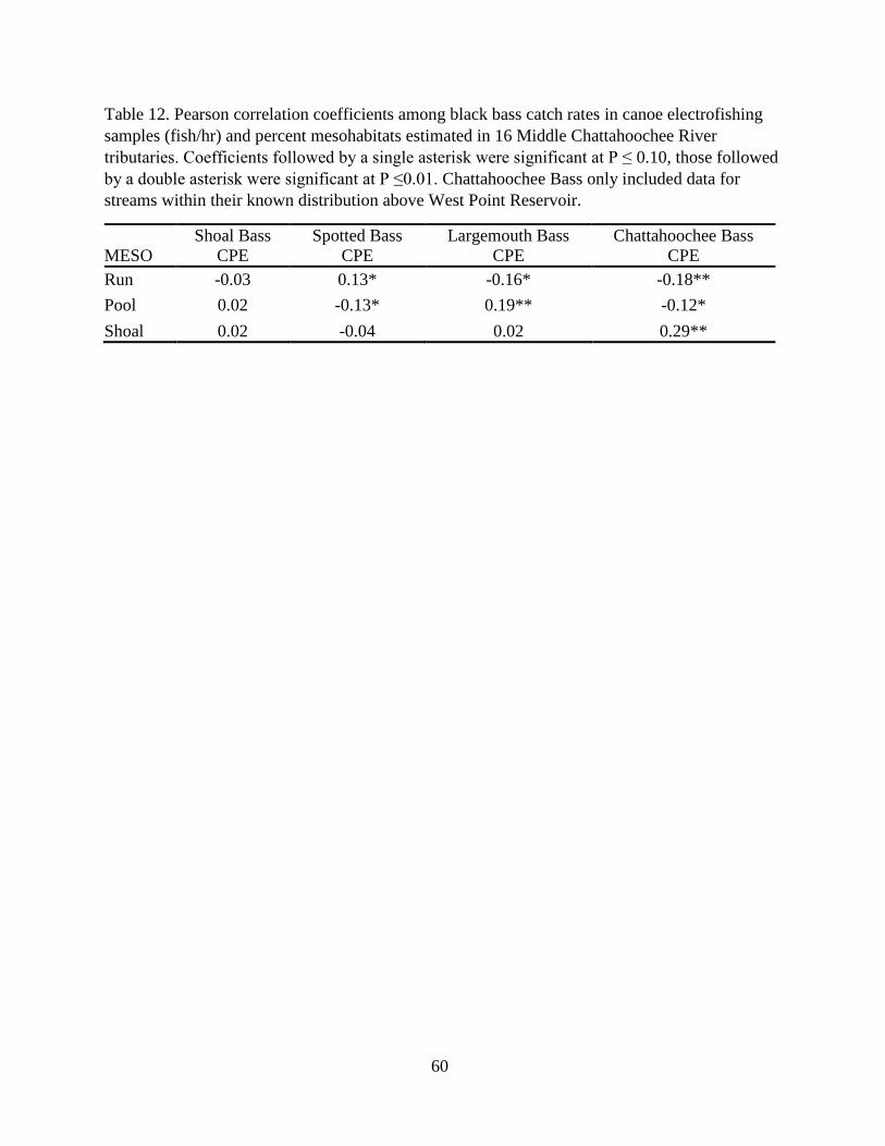
60
Table 12. Pearson correlation coefficients among black bass catch rates in canoe electrofishing
samples (fish/hr) and percent mesohabitats estimated in 16 Middle Chattahoochee River
tributaries. Coefficients followed by a single asterisk were significant at P ≤ 0.10, those followed
by a double asterisk were significant at P ≤0.01. Chattahoochee Bass only included data for
streams within their known distribution above West Point Reservoir.
MESO
Shoal Bass
CPE
Spotted Bass
CPE
Largemouth Bass
CPE
Chattahoochee Bass
CPE
Run -0.03 0.13* -0.16* -0.18**
Pool 0.02 -0.13* 0.19** -0.12*
Shoal 0.02 -0.04 0.02 0.29**

61
Table 13. Black Bass mesohabitat predictive models used to determine the probability of catching a black bass species in each
mesohabitat. Models used black bass presence/absence and estimated mesohabitat data from canoe electrofishing (15-minute
transects) of 16 Middle Chattahoochee River tributaries surveyed in the summer of 2013. Predictive models using a Binomial
distribution of species presence/absence with a random effect of stream. Only significant effects of mesohabitat were shown for each
species. Akaike’s Information Criterion (AIC) is a model selection criterion, corrected Akaike’s Information Criterion (AICc) is a
model selection criterion with a correction for the number of parameters, Bayes Information Criterion (BIC) is another model
selection criterion, and deviance is a quality of fit statistic for a model. No significant models were found for Spotted Bass.
Species Fixed Effects Estimate Std.
Error
z
value Pr(>|z|) AIC AICc BIC -nll deviance df
Shoal Bass
% Shoal 3.397 1.406 2.417 P< 0.05 107.7 107.8 117.9 -50.9 101.7 215
% Run -1.601 0.957 -1.673 P< 0.10 112.7 112.9 122.9 -53.4 106.7 215
Largemouth
Bass
% Run -1.085 0.548 -1.979 P< 0.05 244.8 244.9 254.9 -119.4 238.8 215
% Pool 2.287 0.67 3.412 P< 0.001 236.5 236.7 246.7 -115.3 230.5 215
Chattahoochee
Bass
% Shoal 5.562 1.432 3.885 P< 0.001 72.9 73.3 79.9 -33.5 66.9 92
% Run -4.11 1.348 -3.049 P< 0.01 82.4 82.7 89.3 -38.2 76.4 92
% Pool -9.481 4.484 -2.114 P< 0.05 86 86.4 93 -40 80 92

62
Table 14. Land use areas (km²) for each stream sampled in the Middle Chattahoochee River. Land cover data were collected from
NLCD imagery and analyzed in ArcGIS 10. Areas (km²) of each land cover type are measured for each watershed. Streams were
listed alphabetically and stream abbreviations are listed in Table 1. Forested cover was divided into deciduous (Decid), evergreen
(Everg), and mixed. Wetlands were divided into wooded and herbaceous wetlands (Herba), and herbaceous plants are different
from wetland herbaceous plants.
Developed Forested Agriculture Wetlands
Stream Area Open Low Med High Barren Decid Everg Mixed Shrub Herba Pasture Crop Wooded Herba
CTH 219.9 9.1 2.7 0.7 0.1 0.6 73.3 51.4 0.8 15.2 10.3 53.3 0 1.9 0
DOG 293.5 29.2 15.5 3.1 1.1 1.8 106.7 67.7 0.8 10.7 13.4 36.2 0 2.5 0.1
FSH 811.8 30.3 7.7 0.8 0.3 1.8 207.1 251.2 6.3 74.2 52.6 138.2 0.5 32.4 2.8
HLB 298.1 8.1 1.4 0.1 0 1.1 107 84.3 0.9 33.4 23.8 31 0 5.5 0.3
HWK 284.5 12.6 9.9 2.9 1.5 1 89.9 63 1.9 23.4 20 48.9 0.4 6.7 0.6
LUC 497.9 37.3 18.4 2.3 0.5 1.9 151 91.2 22.9 69.3 15.1 50.2 11.5 19.1 1.5
MTN 253.3 13.9 1.7 0.3 0 0.2 91.7 84.7 1.6 16.5 12.5 13.1 0 12.4 0.2
MUL 836 43.6 8.5 0.9 0.3 1.4 327.6 219 4 66 54.5 72.2 0.1 27.7 1.8
NWR 545 25.4 12 2 1.6 0.8 132.2 192.8 3.8 31 30.5 75.2 0.1 29.3 0.3
OSA 448.1 19.1 5.7 1.2 0.5 1.1 143.8 113.2 4.6 46 27.7 62.1 0.1 19.7 1.1
SNK 184.3 9 4.3 0.4 0.1 0.5 66.1 50.2 0.4 12.8 12.6 20.2 0 2.6 0
STB 256.2 18 9.7 1.5 0.4 2.7 99.9 68 1.7 11.6 14.1 17.4 0.1 6.9 0.2
SWT 991.1 192 158 38.3 16.5 3.1 225.1 171.4 3.7 18.8 29.7 87.4 0 34.8 2.2
UCH 715.7 35.9 10.6 1.2 0.1 0.9 161.2 121.5 59.5 135.5 11.7 86.8 38.9 40.6 2.2
WAC 119.5 3.8 1.7 0.1 0 0.8 35.7 37.7 0.5 10.8 13.3 13.2 0 1.4 0
WHK 315.6 11.2 4.3 0.7 0.2 0.5 99.8 63.2 1.8 36 27.8 59.8 0.1 7.8 1.1
WPG 117.2 5.7 2.7 0.3 0.1 0.1 41 28.4 0.6 6.4 6.2 23.8 0 1 0.1
TOTAL 7187.7 504.2 275 56.8 23.3 20.3 2159.1 1759 115.8 617.6 375.8 889 51.8 252.3 14.5
MEAN 417.2 28.7 15.4 3.2 1.3 1.2 125.7 103.6 6.6 35.8 22.2 51 2.9 14.8 0.8

63
Table 15. Mean land-cover (km²) of streams with a high Shoal Bass population, low Shoal Bass (SHB) population, absent,
comparison of high versus absent, comparison of low versus absent, and comparison of high versus low. Mean land-cover of
streams where Chattahoochee Bass (CHB) are present and absent, and present versus absent. Forested cover was divided into
deciduous (Decid), evergreen (Everg), and mixed. Wetlands were divided into wooded and herbaceous wetlands (Herba), and
herbaceous plants are different from wetland herbaceous areas.
Area
(km²)
Developed
Barren
Forested
Shrub Herba
Agriculture Wetlands
Open Low Med High Decid. Everg Mixed Pasture Crop Wooded Herba
SHB Present 483.2 39.2 23 5 2.1 1.35 149.1 117.4 4.7 36.5 25.6 56.3 1.3 16.2 1.1
SHB Absent 336.6 16.1 6.5 0.9 0.4 1 95.5 83.5 9.8 36.1 17.2 46.6 5.6 12.9 0.5
SHB High 879.6 88.6 58.1 13.3 5.7 2.1 253.3 213.9 4.7 53 45.6 99.3 0.2 31.6 2.3
SHB Low 313.2 18 7.9 1.5 0.5 1 104.4 76.1 4.8 29.4 17 37.9 1.7 9.6 0.6
CHB Present 222.6 12.2 5.3 0.9 0.3 0.8 78.8 56.4 0.7 15.7 13.3 32.9 0 2.7 0.1
CHB Absent 617.2 76.2 58.1 13.7 6.1 1.5 152.4 142.5 3.1 28.6 29.3 74.1 0.1 24 1.2

64
Table 16. Streams were assigned into abundance categories for Shoal Bass (SHB) and
Chattahoochee Bass (CHB) based upon total catch of each species throughout the study.
Streams where > 25 fish were collected were considered high abundance, whereas, those
where <25 fish were collected were considered low abundance. If no fish were collected, the
species was considered absent.
Abundance Classification Land Use Categories
Stream SHB CHB Developed Nat. Ag. Forested
Centralhatchee Absent Present 5.7 69.5 24.2 57.1
Dog Low Present 16.7 68.8 12.3 59.7
Flat Shoals High - 4.8 77.2 17.1 57.2
Hillabahatchee Low Present 3.2 85.6 10.4 64.5
Halawakee Absent - 9.5 72.2 17.3 54.4
Little Uchee Low - 11.7 74.3 12.4 53.2
Mountain Oak Low - 6.3 86.7 5.2 70.3
Mulberry High - 6.4 83.8 8.6 65.9
New River Absent Absent 7.5 77 13.8 60.3
Osanippa Low - 5.9 79.5 13.9 58.4
Snake Absent Present 7.5 78.5 11 63.3
Standing Boy Absent - 11.6 79 6.8 66.2
Sweetwater High Absent 40.9 49 8.8 40.4
Uchee Absent - 6.7 74.4 17.6 47.8
Wacoochee Absent - 4.7 83.2 11 61.8
Wehadkee Absent Absent 5.2 75.3 19 52.2
Whooping Low Present 7.5 71.4 20.3 59.7
MEAN . . 9.5 75.6 13.5 58.4

65
Table 17. Total substrate types (km²) within each mesohabitat of each mapped stream from
side-scan sonar surveys performed during the spring of 2015. Streams are listed from north to
south as they enter the Chattahoochee River.
Stream Substrate Mesohabitat
Pool Riffle Run Shoal Total
Flat Shoals
Creek
Bedrock 0.626 0.074 0.682 3.802 5.184
Boulder 0.398 0.401 1.624 3.764 6.187
Cobble 0.261 0.504 0.494 0.110 1.370
Sand/Gravel 2.945 0.334 36.037 0.064 39.379
Shadow 0.009 0.073 0.521 0.000 0.603
Unsure 0.140 0.000 0.040 0.000 0.179
Mountain Oak
Creek
Bedrock 0.233 0.027 0.280 0.424 0.965
Boulder 0.124 0.068 0.262 0.635 1.088
Cobble 0.153 0.158 0.604 0.099 1.014
Sand/Gravel 0.890 0.015 4.972 0.221 6.098
Shadow 0.008 0.012 0.032 0.003 0.055
Unsure 0.000 0.000 0.000 0.160 0.160
Osanippa Creek
Bedrock 1.298 0.319 2.031 1.491 5.140
Boulder 0.453 0.645 1.899 2.742 5.739
Cobble 0.220 0.257 0.895 0.364 1.736
Sand/Gravel 1.989 0.336 8.240 0.170 10.736
Shadow 0.000 0.000 0.073 0.000 0.073
Unsure 0.000 0.000 0.000 0.000 0.000
Halawakee
Creek
Bedrock 0.647 0.017 0.348 1.127 2.138
Boulder 0.266 1.104 0.796 2.946 5.112
Cobble 0.485 0.907 0.973 0.697 3.063
Sand/Gravel 1.302 0.314 6.057 0.170 7.843
Shadow 0.001 0.129 0.033 0.030 0.194
Unsure 0.000 0.000 0.000 0.053 0.053
Mulberry Creek
Bedrock 1.322 0.093 0.882 4.543 6.839
Boulder 2.330 0.485 2.645 2.459 7.919
Cobble 0.399 0.191 0.805 0.161 1.556
Sand/Gravel 9.239 0.585 39.408 0.977 50.209
Shadow 0.107 0.172 0.468 0.269 1.016
Unsure 0.196 0.102 0.009 0.063 0.370
TOTAL 26.041 7.321 111.112 27.545 172.019

66
Table 18. Percent substrate within each mesohabitat of each mapped stream from side-scan
sonar surveys performed during the spring of 2015. Streams are listed from north to south as
they enter the Chattahoochee River.
Stream Substrate Mesohabitat
Pool Riffle Run Shoal Total
Flat Shoals
Creek
Bedrock 14.3 5.4 1.7 49.1 9.8
Boulder 9.1 28.9 4.1 48.6 11.7
Cobble 6.0 36.4 1.3 1.4 2.6
Sand/Gravel 67.3 24.1 91.5 0.8 74.4
Shadow 0.2 5.2 1.3 0.0 1.1
Unsure 3.2 0.0 0.1 0.0 0.3
Mountain Oak
Creek
Bedrock 16.6 9.8 4.6 27.5 10.3
Boulder 8.8 24.3 4.3 41.1 11.6
Cobble 10.8 56.5 9.8 6.4 10.8
Sand/Gravel 63.2 5.3 80.8 14.4 65.0
Shadow 0.6 4.1 0.5 0.2 0.6
Unsure 0.0 0.0 0.0 10.4 1.7
Osanippa Creek
Bedrock 32.8 20.5 15.5 31.3 21.9
Boulder 11.4 41.4 14.5 57.5 24.5
Cobble 5.6 16.5 6.8 7.6 7.4
Sand/Gravel 50.2 21.6 62.7 3.6 45.8
Shadow 0.0 0.0 0.6 0.0 0.3
Unsure 0.0 0.0 0.0 0.0 0.0
Halawakee
Creek
Bedrock 23.9 0.7 4.2 22.4 11.6
Boulder 9.8 44.7 9.7 58.6 27.8
Cobble 18.0 36.7 11.9 13.9 16.6
Sand/Gravel 48.2 12.7 73.8 3.4 42.6
Shadow 0.0 5.2 0.4 0.6 1.1
Unsure 0.0 0.0 0.0 1.1 0.3
Mulberry Creek
Bedrock 9.7 5.7 2.0 53.6 10.1
Boulder 17.1 29.8 6.0 29.0 11.7
Cobble 2.9 11.7 1.8 1.9 2.3
Sand/Gravel 68.0 35.9 89.1 11.5 73.9
Shadow 0.8 10.6 1.1 3.2 1.5
Unsure 1.4 6.3 0.0 0.7 0.5

67
IX. FIGURES

68
Figure 1. Study area of the Middle Chattahoochee River of Alabama and Georgia. All streams
shown were sampled for habitat at multiple scales and with electrofishing. *Streams where side-
scan sonar surveys were conducted are denoted by an asterisk.

69
---------------------------------------------------------------------------------------------------------------
Figure 2. (TOP) Example image output from side-scan sonar mapping. Picture shows scanning
width at the top left and right in feet, depth in feet, boat speed in miles-per-hour, temperature in
Fahrenheit, latitude and longitude in decimal degrees, time, and date. (BOTTOM) Example
imagery with the ‘collar’ of information removed for later rectification in ArcGIS.

70
Figure 3. (TOP) Image of a control point network for 3 images using side-scan sonar. Points
represent the 30-point networks of 3 images that determine how the images will be warped or
rectified to fit the stream GPS path and connect to adjacent imagery. (MIDDLE) Image of a
control point network with merged images of instream habitats, showing how images are merged
together and follow the stream banks. (BOTTOM) Image of habitat delineation and the final step
in procedure for quantifying instream habitat. Bedrock substrates are black, boulder substrates
are dark grey, cobble substrates are grey, and sand substrates are light grey.

71
Figure 4. Percent of substrate types (defined in Table 2), and percent of rock and wood cover of four mesohabitats sampled using the
point and transect method in 16 Middle Chattahoochee River tributaries in summer 2014. The number of points sampled in each
mesohabitat is defined by N.

72
Figure 5. Stream velocity (m/s) frequency distributions between Shoal Bass and Chattahoochee Bass presence/absence. Distributions
were compared using a K-S test (P< 0.05). Chattahoochee Bass data are from streams within their known range.

73
Figure 6. Stream depth (m) frequency distributions between Shoal Bass and Chattahoochee Bass presence/absence. Distributions were
compared using a K-S test (P< 0.05). Chattahoochee Bass data are from streams within their known range.

74
Figure 7. Stream width (m) frequency distributions between Shoal Bass and Chattahoochee Bass presence/absence. Distributions were
compared using a K-S test (P< 0.05). Chattahoochee Bass data are from streams within their known range.

75
Figure 8. Percent substrate types (defined in Table 2) of Shoal Bass and Chattahoochee Bass presence/absence from backpack
electrofishing surveys of mesohabitats in 16 Middle Chattahoochee River tributaries in summer 2014 (P< 0.10). Chattahoochee Bass
data only from streams within their known range.

76
Figure 9. Percent mesohabitat types (defined in Table 2) of Shoal Bass and Chattahoochee Bass
presence/absence from canoe electrofishing 15-minute transects of stream reaches in 16 Middle
Chattahoochee River tributaries in summer 2013 (P< 0.10). Chattahoochee Bass data only from
streams within their known range.

77
Figure 10. Comparison of mean substrates between point/transect data and side-scan sonar data
from Flat Shoals and Mulberry Creeks, which both have similar-sized watershed areas (811.8-
836 km²). Data were collected for point/transect (PT) surveys in summer 2014 and side-scan
sonar (SSS)surveys in spring 2015.
0.0
0.2
0.4
0.6
0.8p
rop
ort
ion
Flat Shoals Creek
0.0
0.2
0.4
0.6
0.8
Bedrock
SSS
Bedrock
PT
Boulder
SSS
Boulder
PT
Cobble
SSS
Cobble
PT
Sand/Gr
SSS
Sand/Gr
PT
pro
po
rtio
n
Mulberry Creek

78
Figure 11. Comparison of mean substrates between point/transect data and side-scan sonar data
from Mountain Oak and Halawakee Creeks, which both have similar-sized watershed areas
(253.3-284.5 km²). Data were collected for point/transect (PT) surveys in summer 2014 and side-
scan sonar surveys (SSS) in spring 2015.
0.0
0.2
0.4
0.6
0.8p
rop
ort
ion
Mountain Oak Creek
0.0
0.2
0.4
0.6
0.8
Bedrock
SSS
Bedrock
PT
Boulder
SSS
Boulder
PT
Cobble
SSS
Cobble
PT
Sand/Gr
SSS
Sand/Gr
PT
pro
port
ion
Halawakee Creek

79
Figure 12. Comparison of mean substrates between point/transect data and side-scan sonar data
from Osanippa Creek, which has a watershed area that is intermediate to other mapped streams
(448.1 km²). Data were collected for point/transect (PT) surveys in summer 2014 and side-scan
sonar surveys (SSS) in spring 2015.
0.0
0.2
0.4
0.6
0.8
Bedrock
SSS
Bedrock
PT
Boulder
SSS
Boulder
PT
Cobble
SSS
Cobble
PT
Sand/Gr
SSS
Sand/Gr
PT
pro
port
ion
Osanippa Creek

80
Figure 13. Comparison of mean substrates between point/transect data and side-scan sonar data
from mapped streams overall Data were collected for point/transect (PT) surveys in summer
2014 and side-scan sonar surveys (SSS) in spring 2015.
0.0
0.2
0.4
0.6
0.8
Bedrock
SSS
Bedrock
PT
Boulder
SSS
Boulder
PT
Cobble
SSS
Cobble
PT
Sand/Gr
SSS
Sand/Gr
PT
pro
po
rtio
nAll Mapped Streams

81
X. APPENDICES

82
X.1. Side-Scan Sonar Start and End GPS Points.
Appendix 1. Side-scan sonar Middle Chattahoochee River tributary start and end latitude and
longitude in decimal degrees.
Stream Start Lat Start Long End Lat End Long
Flat Shoals 32.881358 -85.077806 32.794239 -85.137466
Mountain Oak 32.741173 -85.068769 32.726271 -85.095011
Osanippa 32.784802 -85.193542 32.831511 -85.147502
Halawakee 32.69751 -85.266742 32.686139 -85.204418
Mulberry 32.695939 -84.913133 32.640596 -85.065272

83
X.2. Point/Transect Sampling Form
SHOAL BASS HABITAT SAMPLING
DATE: STREAM: ___________________
REACH: MSW: MESOHABITAT:_____________
% WOODY COVER: __% ROCK/BOULDER:_________/__________
START : WPT: LAT: __LONG:____________________
STOP : WPT: LAT: LONG:___________________
WIDTH MEASUREMENTS (mm)
TR PT BF CUR DEP VEL SUB 1 2 3 4 5 6 7

84
X.3. Point/Transect Electrofishing Form

85
X.4. Canoe Hand-held Electrofishing Sampling Form

86
X.5. Land Cover Classifications
A Revision of : A Land Use And Land Cover Classification System For Use With Remote Sensor Data (Anderson, et al. 1976)


