BIO4503
Experimental designs – RCTs
• The central them of this session will be the gold-standard in research; the Randomized Clinical Trail (RCT). Here we will cover: description of the general design, characteristics and aims and types and variations.
• We will also introduce the study and analysis of confounders and biases and the most common sampling strategies used for RCTs and other research designs
Dr Carmen [email protected]

LEVELS OF RESEARCH (and THEIR BASIC DESIGNS)
STRUCTURAL FEATURES
EXPERIMENTAL QUASI-EXPERIMENTAL NON-EXPERIMENTAL
Manipulation Variables are actively
manipulated
Variables may be actively manipulated
None
Control High degree with a separate control
group
Restricted, sometimes no-control group
None or minimal
Randomisation Random assignment to level of the manipulated
variable(s)
None None
Examples of designs
Randomized Clinical Trial
(explanatory variables)
- Case-control study- Cohort study- Non-equivalent control group design- Interrupted time-series design- Single system design
- Surveys- Qualitative studies(Exploratory and
descriptive variables)

EXPERIMENTAL DESIGNS. Randomised Clinical TrialsDEFINITIONS OF RCTs
Bowling A: “Classic experiment in sciences. It involves the random allocation of participants between experimental group(s) whose members receive the treatment/intervention to be tested, and control group(s) whose members receive the standard treatment or a placebo (dummy) treatment (…). The outcome of the groups is compared”.
Sim & Wright: “Longitudinal (prospective) design in which an intervention variable is manipulated in order to determine quantitatively its effect on one or more outcome variables, other extraneous variables having been controlled for”

EXPERIMENTAL DESIGNS. Randomised Clinical TrialsBasic operational aspects:
• Entities or variables to examine are quantitative• The conditions to examine such variables are control,
manipulation and randomisation.• The sources of the data we need will be, will be at least
two groups and the comparison of results (outcome variables) between the two groups will be the main finding of the study.
• The time-points for data collection will always be longitudinal prospective
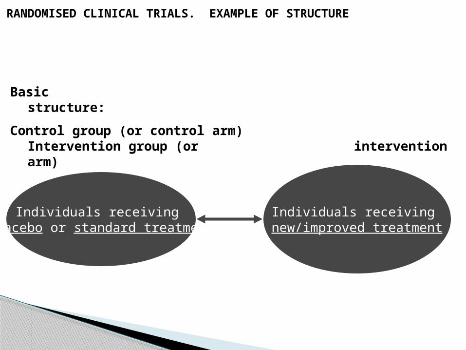
RANDOMISED CLINICAL TRIALS. EXAMPLE OF STRUCTURE
Basic structure:
Individuals receiving placebo or standard treatment
Individuals receiving new/improved treatment
comparison
Control group (or control arm) Intervention group (or intervention arm)

RANDOMISED CLINICAL TRIALS. EXAMPLE OF STRUCTURE
comparison
One more step: E.g.: RCTs comparing the effect of different doses of a given treatment on the outcome variable
G1:30–50 mg/day
methadone
G2:50-80 mg/day
methadone
G3:30–50 mg/day
Methadone + CBT
G4:50-80 mg/day
Methadone +CBT
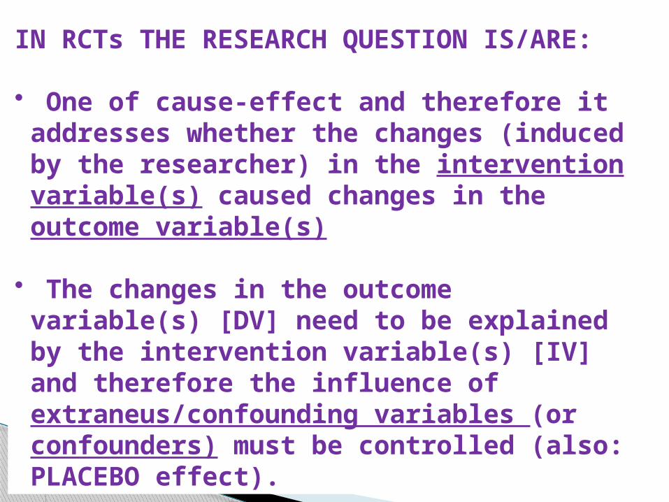
IN RCTs THE RESEARCH QUESTION IS/ARE:
• One of cause-effect and therefore it addresses whether the changes (induced by the researcher) in the intervention variable(s) caused changes in the outcome variable(s)
• The changes in the outcome variable(s) [DV] need to be explained by the intervention variable(s) [IV] and therefore the influence of extraneus/confounding variables (or confounders) must be controlled (also: PLACEBO effect).

Phase I: Tests for effects of new drugs in health volunteers or patients unresponsive to usual therapies.
Subject of study: pharmacokinetics and pharmacodynamics of a new drug in the human body
Phase II: Tests for dose-response curves in small groups of patients with a given disease.
Phase III: Tests for effects in a large population against a placebo or a standard therapy. Considered the landmark study for drugs. Results might gain licence for a drug to be prescribed.
Phase IV: Tests long-term safety and drug interactions in larger groups of patients. Also know as “post-marketing phase”
CLINICAL PHASES OF RCT

MAIN TWO TYPES OF RCTs
a. Explanatory RCT
• Seeks to determine the effect of an specific intervention in absolute terms
• Compare the effect of an intervention with a placebo• It seeks to measure the efficacy of an intervention• Usually includes few measures of effect
b. Pragmatic RCT
• Seeks to determine the effect of an specific intervention in relative terms
• Compare the effect of a new/improved intervention against the standard intervention
• It seeks to measure the effectiveness• Usual analysis will be intention-to-treat• Usually use a wide range of outcome measures

MAIN DESIGNS OF RCT
1. Parallel-group trial design
• One group receiving placebo or standard treatment and another group receiving a new or enhanced treatment
2. Crossover trials
• Subjects are randomised to different sequences of treatments but all patients will eventually get all treatments in a varying order.
• In this case, each patient is his own control.
3. Factorial trials
• Factorial design randomised patients to more than one treatment-comparison group
4. Cluster randomised trials
• Are performed when larger groups of patients (e.g.: Patients of a single hospital) are randomised instead of individual patients.

Given what is at stake in RCTs the study of confounders and biases and how to control and prevent them respectively, is crucial.
WHAT IS A CONFOUNDER?
WHAT IS BIAS?

CONFOUNDERS vs. BIASES
Confounders
• Are variable(s) that affect the outcome variables(s)
• Their effect will be differential between intervention and control groups
• It is because this different effect of the confounding variable on the control and the intervention group, that its effects can be “confounded” with those produced by the intervention variable(s)
• That’s why confounders are threats to the internal validity of a trial
• However values in the outcome variable(s) can be perfectly accurate
• If a confounding variable would affect the control and intervention groups equally:
- There will be no confounding variable and no confounding effect regarding the relative differences between the groups.
- Still the magnitude of the change in the outcome variable(s) could not longer be attributed to the intervention variable(s)

CONFOUNDERS vs BIASES
Biases
• Factors that cause systematic error in the measurement of the outcome variable(s).
• Bias effect prevents from extracting the true value of the outcome variable(s)

CONTROLLING FROM CONFOUNDERS AND BIASES. METHODS
• Simple randomisation
• Stratified randomisation
• Specification
• Minimisation
• Blinding
• Concealment

RANDOMISATION
• It is the main mechanism in RCT to control for the effect of confounders
• It consists in allocating subjects to the groups by a chance mechanism that will give each individual equal chance [equal probability] of been allocated to either group.
• In the simple randomisation the underlying assumption: different characteristics (age, gender, severity of the addiction…) (potential confounders) will be randomly distributed among the groups and therefore their potential influence on the outcome variable(s) will be equalized.
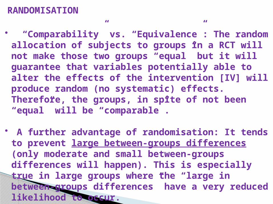
RANDOMISATION
• “Comparability” vs. “Equivalence”: The random allocation of subjects to groups in a RCT will not make those two groups “equal” but it will guarantee that variables potentially able to alter the effects of the intervention [IV] will produce random (no systematic) effects. Therefore, the groups, in spite of not been “equal” will be “comparable”.
• A further advantage of randomisation: It tends to prevent large between-groups differences (only moderate and small between-groups differences will happen). This is especially true in large groups where the “large in between-groups differences” have a very reduced likelihood to occur.

RANDOMISATION• Randomisation won’t diminish the heterogeneity of the
sample as a whole.
• Defining acceptable and desirable levels of heterogeneity should be approached in the sampling strategy.
• Best option to randomise subjects: computer generated random numbers.
• Other methods (e.g.: to allocate patients to the group according to their medical record number) are not random but hapzard methods
• Disclosing the allocation of each individual. Two main methods of treatment allocation: Opaque envelopes & Coordinating centre

STRATIFIED RANDOMISATION
• Simple randomisation does not guarantee equal number of patients (unrestricted randomisation method). To achieve the goal of “equal no. of subjects in each group” we used stratified randomisation.
• Stratification is a restricted method of randomisation (ensures equal number of patients in each group at all times of randomisation).
• Further more [and beyond the goal of “equal no. of subjects per group”, stratified randomization refers to the situation in which strata are constructed based on values of prognostic variables and a randomization scheme is performed separately within each stratum.
• In other words…it consists on dividing the sample, before the randomisation, into strata that will represent the different levels of the potential confounder(s) and then randomise patients from within each group.
STRATIFIED RANDOMISATION
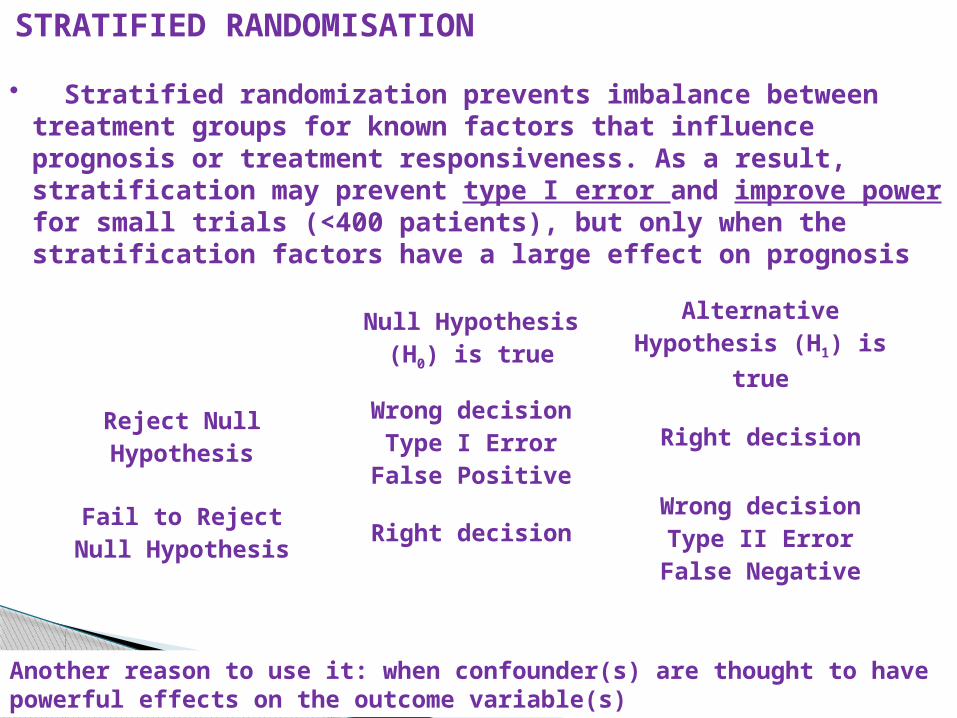
• Stratified randomization prevents imbalance between treatment groups for known factors that influence prognosis or treatment responsiveness. As a result, stratification may prevent type I error and improve power for small trials (<400 patients), but only when the stratification factors have a large effect on prognosis
Null Hypothesis (H0) is true
Alternative Hypothesis (H1) is
true
Reject Null Hypothesis
Wrong decisionType I Error
False PositiveRight decision
Fail to Reject Null Hypothesis Right decision
Wrong decisionType II Error
False Negative
Another reason to use it: when confounder(s) are thought to have powerful effects on the outcome variable(s)
STRATIFIED RANDOMISATION. example
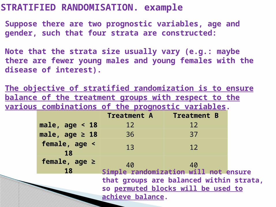
Treatment A Treatment Bmale, age < 18 12 12 male, age ≥ 18 36 37 female, age <
18 13 12
female, age ≥ 18 40 40
Suppose there are two prognostic variables, age and gender, such that four strata are constructed:
Note that the strata size usually vary (e.g.: maybe there are fewer young males and young females with the disease of interest).
The objective of stratified randomization is to ensure balance of the treatment groups with respect to the various combinations of the prognostic variables.
Simple randomization will not ensure that groups are balanced within strata, so permuted blocks will be used to achieve balance.

STRATIFIED RANDOMISATION [cont]Open cohorts and randomisation
• Important feature: use of random blocks which ensures that equal numbers of patients within each stratum are randomised to each intervention.
• In other words, it guarantees that treatments will be balanced after a given block size.
• Example: In the block is size=4, after 4 randomisations we will have 2 patients on treatment A and 2 on treatment B.
• Problem: by the end of the process the allocation is rather predictable.• To overcome the problem:
• Don’t disclose information on the blocks to trialists [blind them].• Use a random permuted blocks protocol: Several block sizes are
used [e.g.: blocks size 4, blocks size 6 and blocks size 8] and a each consecutive block size is chosen at random

Example of randomisation with permuted blocks
Block size = 4 2 Treatments A,B
Possible combinations: AABB, ABBA , ABAB, BBAA, BAAB, BABA
For each block, randomly choose one of the six possible arrangements: AABB, ABAB, BAAB, BABA, BBAA, ABBA
Randomize groups of 4 patients to each block
ABAB BABA ......
Patients 1 2 3 4 5 6 7 8 9 10 11 12
STRATIFIED RANDOMISATION
Close cohorts and randomisation
• Another mechanism to ensure equal distribution of confounders is the match of sets of participants.
• Consists in matching sets of participants on one or more confounding variable and then randomise them.
• It is another form of restricted randomisation
• The number of matched participants will correspond to the number of arms in the trial.
• Can only be done with known confounders
• No feasible with more than three arms RCT
SPECIFICATION
• Another mechanism to deal with confounders.
• Consists in limiting participants to a certain value or range of values of an specific variable previously identified as confounder.
• Suitable for open and close cohorts
• Questions the external validity of the experiment.
MINIMISATION
• Another mechanism to deal with confounders.
• Consists in allocating each participant to the arms of the RCT no randomly but with the aim of reaching between-groups “homogeneity” regarding previously identified confounders.
• Suitable for open cohorts
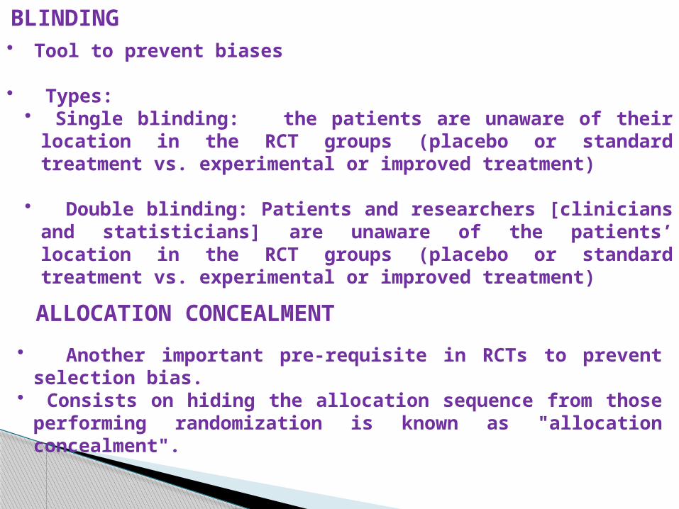
BLINDING• Tool to prevent biases
• Types:• Single blinding: the patients are unaware of their location in the RCT
groups (placebo or standard treatment vs. experimental or improved treatment)
• Double blinding: Patients and researchers [clinicians and statisticians] are unaware of the patients’ location in the RCT groups (placebo or standard treatment vs. experimental or improved treatment)
ALLOCATION CONCEALMENT
• Another important pre-requisite in RCTs to prevent selection bias.• Consists on hiding the allocation sequence from those performing
randomization is known as "allocation concealment".
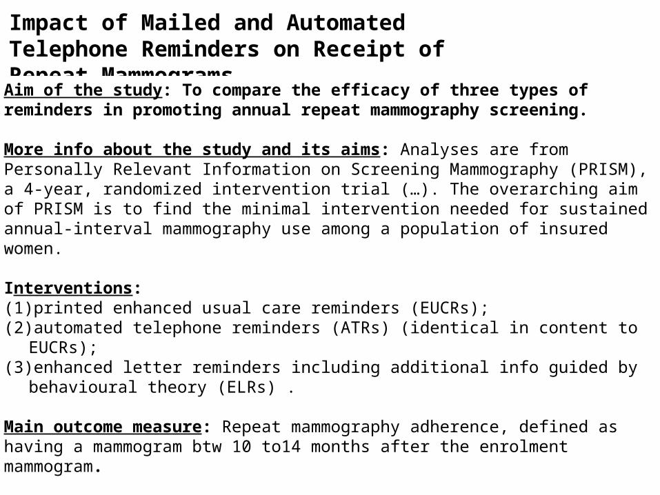
Impact of Mailed and Automated Telephone Reminders on Receipt of Repeat Mammograms
Aim of the study: To compare the efficacy of three types of reminders in promoting annual repeat mammography screening.
More info about the study and its aims: Analyses are from Personally Relevant Information on Screening Mammography (PRISM), a 4-year, randomized intervention trial (…). The overarching aim of PRISM is to find the minimal intervention needed for sustained annual-interval mammography use among a population of insured women.
Interventions: (1) printed enhanced usual care reminders (EUCRs); (2) automated telephone reminders (ATRs) (identical in content to EUCRs);(3) enhanced letter reminders including additional info guided by behavioural theory
(ELRs) .
Main outcome measure: Repeat mammography adherence, defined as having a mammogram btw 10 to14 months after the enrolment mammogram.
Population: Eligible participants had a previous mammogram within a specified window and were due for their next mammogram.
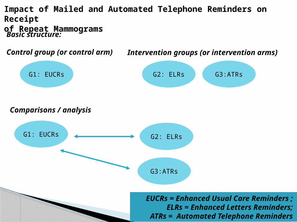
Basic structure:
Control group (or control arm)
G2: ELRs
Impact of Mailed and Automated Telephone Reminders on Receiptof Repeat Mammograms
Intervention groups (or intervention arms)
G1: EUCRs G3:ATRs
Comparisons / analysis
G1: EUCRs G2: ELRs
G3:ATRs
EUCRs = Enhanced Usual Care Reminders ; ELRs = Enhanced Letters Reminders;
ATRs = Automated Telephone Reminders
G3:ATRs

BIO4503.
SAMPLING STRATEGIES AND TECHNIQUES
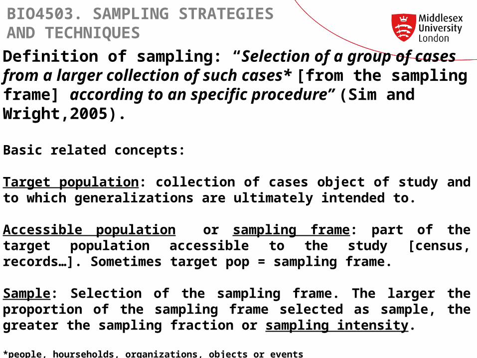
Definition of sampling: “Selection of a group of cases from a larger collection of such cases* [from the sampling frame] according to an specific procedure” (Sim and Wright,2005).
Basic related concepts:
Target population: collection of cases object of study and to which generalizations are ultimately intended to.
Accessible population or sampling frame: part of the target population accessible to the study [census, records…]. Sometimes target pop = sampling frame.
Sample: Selection of the sampling frame. The larger the proportion of the sampling frame selected as sample, the greater the sampling fraction or sampling intensity.
*people, hourseholds, organizations, objects or events
BIO4503. SAMPLING STRATEGIES AND TECHNIQUES
Sampling units = individual cases of the sample
Sample statistic = point estimate of the corresponding population parameter [average age in the sample = sample statistic vs. average age in the population = population parameter
Representativeness: Extend to which characteristics of the accessible population are reflected in the sample at the same level and proportions. If sample is representative it secures external validity.
Basic related concepts [cont]:

Sampling strategies. Types:
A. Empirical representativeness
1. Simple random sampling [Probabilistic]2. Systematic sampling with random start [Probabilistic]3. Cluster sampling [Probabilistic]4. Stratified random sampling [Probabilistic]5. Quota sampling [no-probabilistic]
B. Theoretical representativeness1. Judgmental sampling
2. Convenience sampling
•

SAMPLING STRATEGIES. TYPES
A. Empirical representativeness For descriptive and explanatory RQs
Sampling strategies [Probabilistic* and no-probabilistic**]1. Simple random sampling [Probabilistic]2. Systematic sampling with random start [Probabilistic]3. Cluster sampling [Probabilistic]4. Stratified random sampling [Probabilistic]5. Quota sampling [no-probabilistic]
• * The probability of selection of each case is known and lies [but doesn’t include] between 0 and 1.
** The probability of selection of each case is the researcher’s decision. It might be or no known. If known is always 0 or 1

Sampling strategies. Types:
B. Theoretical representativeness
Used in exploratory RQs [qualitative designs]
Sampling strategies [No-probabilistic**]
1. Judgmental sampling
2. Convenience sampling
**The probability of selection of each case is the researcher’s decision. It might be or no known. If known is always 0 or 1
1. SIMPLE RANDOM SAMPLING
• Sampling frame is known
• Units have an equal, and ≠ 0 or 1, chance of being selected - Draws must be independent [the selection of a unit must not affect the chances of other unit been selected]- The sampling frame must be exhaustive- All units must be individually identified
• In theory, no particular attribute has more chances to be represented in the sample than other.
- But, more frequent attributes will be more represented in the final sample
- However, all attributes have the same chance of been represented in the sample in similar proportions to that found in the population.
- There is not guarantee that the representation of attributes in the sample will match the representation in the population. That will vary from sample to sample [sampling error]

2. SYSTEMATIC SAMPLING WITH RANDOM START [SYSTEMATIC SAMPLING]
• Sampling frame is known• Only the first unit is chosen at random• Subsequent units are chosen at intervals• The interval can be determined by dividing the sampling frame by
sample size:
E.g.: Sample size = 134Sampling frame = 2,300Interval = 2,300/134 = 17.16 = 17Therefore:The first unit [in red] will be randomly selectedThe second unit [in yellow] will be the one following the 1st after 16 units.
1 2 3 4 5 6 7 8 9 10 11 12 13 14 15 16 17 18 19 20 21 22 23 24 25 26
27 28 29 30 31 32 33 34 35 36 37 38 39 40 41 42 43 44 45 46… 134

3. CLUSTER SAMPLING
When:• Sampling frame is unknown• Direct contact with sample units is needed
Mechanics: • A number of clusters of sampling units are selected• Units are sampled within each cluster Variation: multistage cluster sampling• further clusters are drawn from initial clusters • further sampling units are sampled from within
subsequent clusters
Condition: Clusters must be as heterogonous as possibleMembership to each cluster must be mutually exclusive
3. CLUSTER SAMPLING [CONT]
Selection of clusters and units:
Clusters are not randomly selectedUnits are randomly selectedTherefore: final sample is semi-random
Also to consider: Units from different clusters must be fully independent [re the attributes we want to measure]
Advantage: sample size smaller than in simple randomizationDisadvantage: especially in multistage: sample error is added to each stage

4. STRATIFIED RANDOM SAMPLING
Mechanics:• Frame sampling [population] divided into strata [e.g.:
capital city vs. no-capital city]• Randomization applied from within each stratum.
Types:
Proportionate: Sample size within each stratum preserves the representation of certain attributes in the population [e.g.: in stratum “city” there are 80% senior staff vs. 20% “junior staff”. If sample size within stratum requires n=30; 24 = senior staff and 6 = junior staff]
Disproportionate: Sample size within each stratum does not preserve the representation of certain attributes in the population [e.g.: in stratum “city” there are 80% senior staff vs. 20% “junior staff”. We are interested in knowing equally about junior and senior staff. Sample size within stratum requires n=30; 15 = senior and 15 = junior]
4. STRATIFIED RANDOM SAMPLING [CONT]
Advantage:• Usually more representative than random sampling [it
incorporates between-stratum variation]
Conditions:
• Strata should be homogeneous in content [e.g.: in each stratum we have both senior and junior staff] but heterogeneous respect to each other [in each stratum we have different proportions of junior and senior staff]
• Stratification variable(s) must be theoretically relevant [has to do with the main issues investigated in the study: it must be associated with an outcome variable/s]

5. QUOTA SAMPLING
Main concepts:• It is a no-probabilistic* sampling strategy• Still aims to achieve statistical representativeness• Sampling units are not randomized but chosen to fulfill
quota
Defining quota. Mechanics:
• 1st: definition of quota controls: variables on which statistical representativeness is believed to be important.
• 2nd definition of quota specification: number of individuals needed in each quota control
* The probability of selection of each case is the researcher decision. It might be or no known. If known is always 0 or 1

5. QUOTA SAMPLING [CONT]
Selecting sampling units. Mechanics: Direct invitation. Once each quota is filled no more individuals [potential sampling units in that quota] are approached
Advantages: • Don’t need exhaustive sample frame• No a priori selected sampling units [therefore no problem with refusal
to participate in the study]
Disadvantages: • Methodologically weak: sample is representative only in terms of the
quota controls [it might be atypical of the population] • Sampling error cannot be calculated and statistical tests that assume
random selection [parametric] cannot be used• Selection bias always present
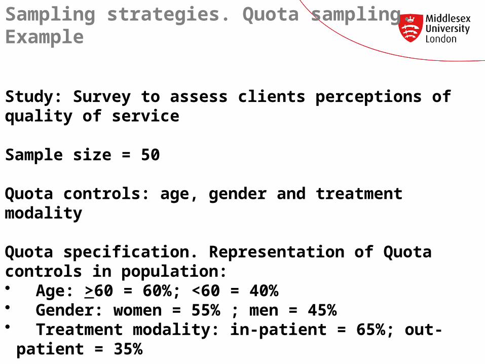
Sampling strategies. Quota sampling. Example
Study: Survey to assess clients perceptions of quality of service
Sample size = 50
Quota controls: age, gender and treatment modality
Quota specification. Representation of Quota controls in population:• Age: >60 = 60%; <60 = 40%• Gender: women = 55% ; men = 45%• Treatment modality: in-patient = 65%; out-patient = 35%

B. SAMPLING STRATEGIES. THEORETICAL REPRESENTATIVENESS
• For exploratory RQs • Sampling strategies: Purposive sampling [No-
probabilistic**]
• Types:
1. Judgmental sampling
2. Convenience sampling
** The probability of selection of each case is the researcher’s decision. It might be or no known. If known is always 0 or 1
1. JUDGMENTAL SAMPLING
• Any method based on the researcher’s judgment on what units are relevant to be sampled.
• Some reasons to include cases [people]:• They have the necessary knowledge• They have the relevant experience• They are part of the social structure or process focus of
the study
• Reasons no to draw a statistically representative sample:• A sampling frame can not be constructed• Cases are very rare [difficult to trace]• The study is too in-depth to handle a large sample.• Doesn’t aim at statistical generalization
1. JUDGMENTAL SAMPLING [CONT.]
• The sample might be recruited in parallel with data collection [e.g.: snowball sampling]
• The rationale for sampling might be parallel to data collection [identification of new “types of cases” as result of interim analysis] [usual in grounded theory studies]
• Cases are part of the social structure or process focus of the study
• Cases might not necessarily be typical [interest in atypical cases or outliers]

2. CONVENIENCE SAMPLING
• Any method where sampling units are draw on the basis of their availability.
• Theoretical and empirical representativeness are both compromised.
• Theoretical representativeness can be achieved if availability is not the only criterion to select cases
• Self-selection bias often introduced.
RECOMMENDED READING
- Sim J & Wright C. (2000) CHAPTER 8
- Bowling A. (2005) CHAPTER 8 [until page 199]
- Burns RB (2000) CHAPTER 12
- Argyrous G (2000) CHAPTER 12 [hardcopy given to you]
RECOMMENDED READING
• Gordis L. (2009) EPIDEMIOLOGY. CHAPTERS 7 and 8 and SECTION II [it includes chapters 9 to 16]
• Jadad A.R. (1998) Randomised controlled trials: a user's guide. London: British Medical Association, 1998.
• Pocock S.J. (1983) Clinical trials: a practical approach. Chichester: Wiley, 1983
• Sim J & Wright C. (2000) CHAPTER 7 and 8• McCancea, DR (2010) Vitamins C and E for prevention of pre-eclampsia in
women with type 1 diabetes (DAPIT): a randomised placebo-controlled trial. Lancet. 2010 July 24; 376(6736): 259–266 [uploaded in UEL+]
• Wang D. Clinical Trials. A practical guide to design, analysis and reporting. (2006) CHAPTERS 1,2,6, 7, 8, 9, 10, 11 AND 15
• CONSORT STATEMENT website: http://www.consort-statement.org/consort-statement/overview/
INTRODUCTION TO STATISTICS FOR HEALTH RESEARCH AND EPIDEMIOLOGY
- DESCRIPTIVE STATISTICS- INFERENTIAL STATISTICS
ANALYSING QUANTITATIVE DATA: STATISTICS
Main two types
a. Descriptive statistics
• Consist of graphical and numerical techniques for summarising data (Burns, 2000).
• Measures for nominal data• Measures of central tendency• Measures of dispersal or variability
b. Inferential statistics
• Consist of procedures for making generalisations about characteristics of a population based on information obtained from a sample taken from a population (Burns, 2000).

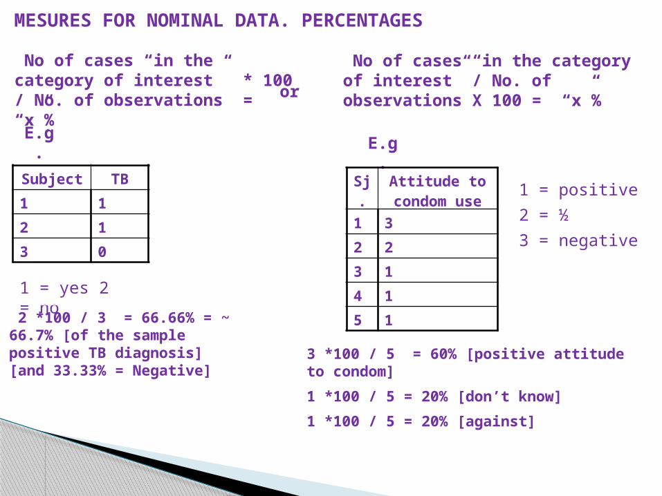
MESURES FOR NOMINAL DATA. PERCENTAGES
• Nominal variables don’t accept arithmetic operations beyond the count.
• Both nominal and categorical variables are discrete (measured as discrete variables)
• Way to deal with large number of numbers (in discrete data): turn it into percentages.
• Continuous variables can also be turned into %s!
MESURES FOR NOMINAL DATA. PERCENTAGES
Subject TB
1 1
2 1
3 0
1 = yes 2 = no
No of cases “in the category of interest” * 100 / No. of observations = “x”%
2 *100 / 3 = 66.66% = ~ 66.7% [of the sample positive TB diagnosis] [and 33.33% = Negative]
No of cases “in the category of interest” / No. of observations X 100 = “x”%or
E.g.E.g.
Sj.
Attitude to condom use
1 3
2 2
3 1
4 1
5 1
1 = positive
2 = ½
3 = negative
3 *100 / 5 = 60% [positive attitude to condom]
1 *100 / 5 = 20% [don’t know]
1 *100 / 5 = 20% [against]

MESURES FOR NOMINAL DATA. PERCENTAGES
PERCENTAGE : No of cases “in the category of interest” *100 / No. of cases = “x”%
VALID PERCENTAGE: No of cases “in the category of interest”*100 / No. of observations = “x”%
COMULATIVE PERCENTAGE: No of cases “in the category of interest” + No of cases in the previous category” x 100 / No. of observations = “x”%
Attitude towards condome use
3 60.0 60.0 60.0
1 20.0 20.0 80.0
1 20.0 20.0 100.0
5 100.0 100.0
positive
don't know
negative
Total
ValidFrequency Percent Valid Percent
CumulativePercent
Attitude towards condome use
3 50.0 60.0 60.0
1 16.7 20.0 80.0
1 16.7 20.0 100.0
5 83.3 100.0
1 16.7
6 100.0
positive
don't know
negative
Total
Valid
999Missing
Total
Frequency Percent Valid PercentCumulative
Percent
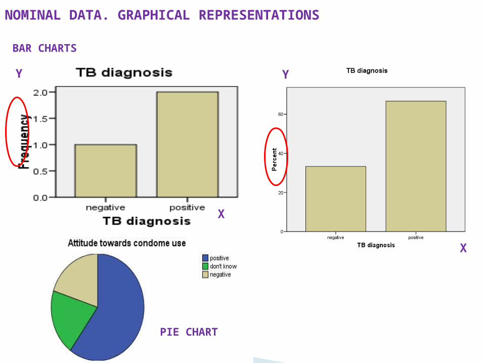
NOMINAL DATA. GRAPHICAL REPRESENTATIONS
X
Y
X
Y
BAR CHARTS
PIE CHART

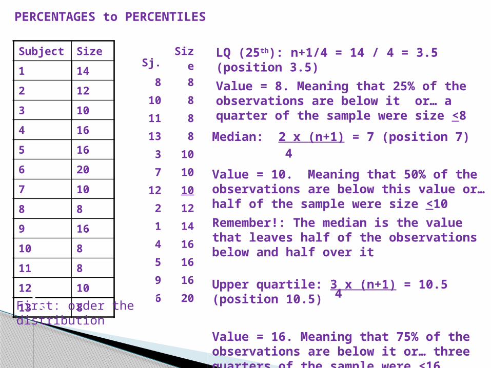
PERCENTAGES to PERCENTILES
PERCENTILES
Def: Value of a variable below which a certain percent of observations fall.
The usual suspects:
Lower quartile: 25th percentile
Median: 50th percentile
Upper quartile: 75th percentile
To locate them: First order the distribution [descendent order]
Lower quartile: n+1
Median: 2 x (n+1) or 50 x (n+1)
Upper quartile: 3 x (n+1) or 75 x (n+1)
4 100
4
1004
Subject Size
1 14
2 12
3 10
4 16
5 16
6 20
7 10
8 8
9 16
10 8
11 8
12 10
13 8
Median: 2 x (n+1) = 7 (position 7)
Value = 10. Meaning that 50% of the observations are below this value or… half of the sample were size <10
Remember!: The median is the value that leaves half of the observations below and half over it
LQ (25th): n+1/4 = 14 / 4 = 3.5 (position 3.5)
Value = 8. Meaning that 25% of the observations are below it or… a quarter of the sample were size <8
Sj. Size
8 8
10 8
11 8
13 8
3 10
7 10
12 10
2 12
1 14
4 16
5 16
9 16
6 20 Upper quartile: 3 x (n+1) = 10.5 (position 10.5)
Value = 16. Meaning that 75% of the observations are below it or… three quarters of the sample were <16
PERCENTAGES to PERCENTILES
First: order the distribution4
4

ANALYSING QUANTITATIVE DATA: STATISTICS
Main two types
a. Descriptive statistics
• Consist of graphical and numerical techniques for summarising data (Burns, 2000).
• Measures for nominal data• Measures of central tendency• Measures of dispersal or variability
b. Inferential statistics
• Consist of procedures for making generalisations about characteristics of a population based on information obtained from a sample taken from a population (Burns, 2000).

DESCRIPTIVE STATISTICS. MESURES OF CENTRAL TENDENCY
First procedures for summarising data. They are: MEAN, MEDIAN and MODE
MEDIAN (or percentile 50)Def: Is the central value of a distribution. The only statistic that disregards extreme valuesE.g.: 23 14 67 45 56E.g.: 22 1 100 15 31 7 [100+15/2 = 57.5]
MODEDef: Is the most frequently occurring value of a distributionE.g.: 23 14 23 45 56 Mo = 23E.g.: 23 1 23 1 31 7 Mo = 1 and 23
MEAN (also known as “average”)
Def: Mean [M or x ] [µ if population instead of a sample] is the sum [Σ] of all scores/observations [X] divided by the number of cases [n]
x= ΣX/NThe only statistic that reflects the influence of all observations in the distribution
E.g.: 23 14 67 45 56 = 205/5 = 41
Subject Size
1 14
2 12
3 10
4 16
5 16
6 20
7 10
8 8
9 16
10 8
11 8
12 10
13 8
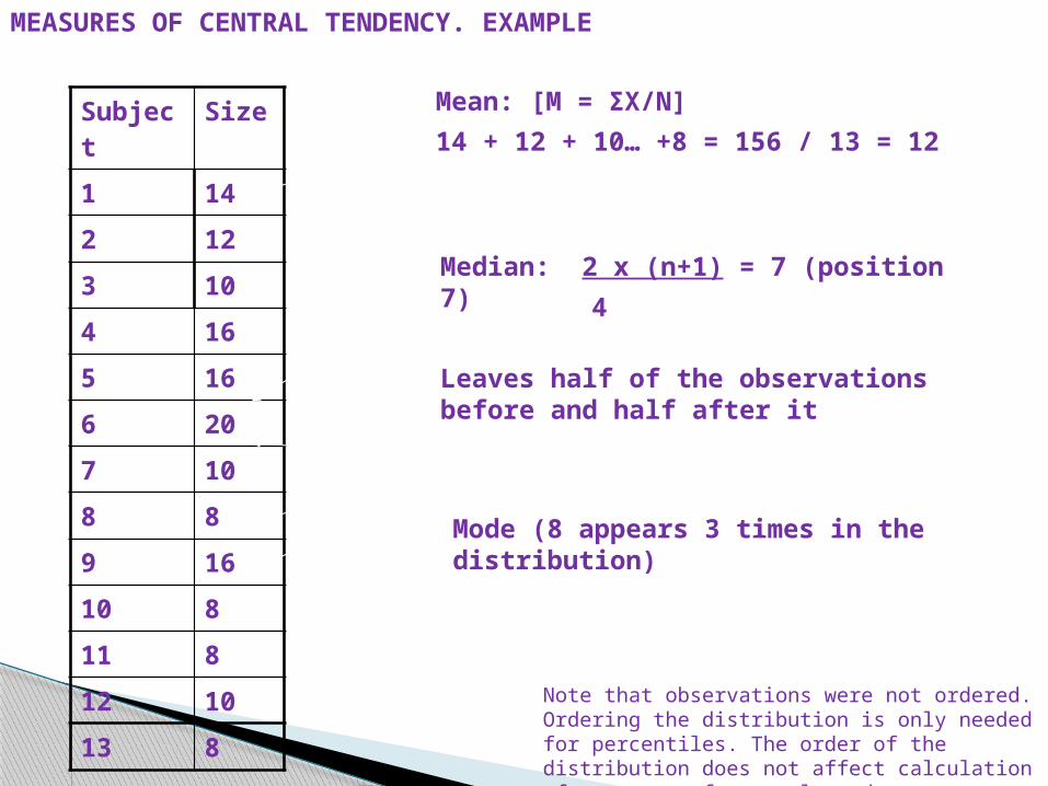
Mean: [M = ΣX/N]
14 + 12 + 10… +8 = 156 / 13 = 12
Mode (8 appears 3 times in the distribution)
Median: 2 x (n+1) = 7 (position 7)
Leaves half of the observations before and half after it
4
Note that observations were not ordered. Ordering the distribution is only needed for percentiles. The order of the distribution does not affect calculation of measures of central tendency
MEASURES OF CENTRAL TENDENCY. EXAMPLE

DESCRIPTIVE STATISTICS. MEASURES OF CENTRAL TENDENCY. GRAPHICAL REPRESENTATIONS
Box plots
Used to present the median and interquartile range of a distribution
0
5
10
15
20
25
1
Q1 (25%)
Min
Median
Max
Q3 (75%)
Statistics
Q1 (25%) 8
Min 8
Median 10
Max 20
Q3 (75%) 16

ANALYSING QUANTITATIVE DATA: STATISTICS
Main two types
a. Descriptive statistics
• Consist of graphical and numerical techniques for summarising data (Burns, 2000).
• Measures for nominal data• Measures of central tendency• Measures of dispersal or variability
b. Inferential statistics
• Consist of procedures for making generalisations about characteristics of a population based on information obtained from a sample taken from a population (Burns, 2000).
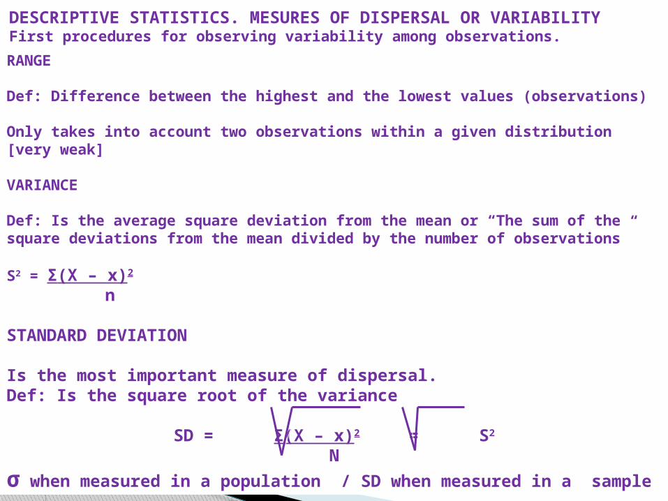
RANGE
Def: Difference between the highest and the lowest values (observations)
Only takes into account two observations within a given distribution [very weak]
VARIANCE
Def: Is the average square deviation from the mean or “The sum of the square deviations from the mean divided by the number of observations”
S2 = Σ(X – x)2
n
STANDARD DEVIATION
Is the most important measure of dispersal.Def: Is the square root of the variance
SD = Σ(X – x)2 = S2
N
σ when measured in a population / SD when measured in a sample
DESCRIPTIVE STATISTICS. MESURES OF DISPERSAL OR VARIABILITYFirst procedures for observing variability among observations.

VARIANCE AND STANDARD DEVIATION. HOMEWORK*
Calculate V and SD of survival to cancer in a sample of seven individuals
Subject Survival [years]
1 6.00
2 5.40
3 3.60
4 7.40
5 10.00
6 1.30
7 0.80
S2 = Σ(X – M)2 N
SD = Σ(X – M)2 = S2
N
* Next session one student will be asked to present his/her calculations and results!
INFERENTIAL STATISTICS (UNIVARIATE, BIVARIATE AND
MULTIVARIATE ANALYSIS)

- We estimate values of parameters (e.g.: mean) from a sample extracted from a population. But how sure are we that the value obtained from the sample (point estimate) is good enough for the whole population?
- To answer such question we use, among other statistics, the CONFIDENCE INTERVAL (CI)
- it can be defined as: “A range that contains the true value of the estimated parameter, if repeated sampling of the population were performed”.
- The 95% confidence interval (CI) is a range that contains the true value of the estimated parameter 95% of the times.
- A narrow range indicates an estimate that is more precise. Small sample sizes lead to less precise estimates and wider CI.
INFERENTIAL STATISTICS. FROM THE SAMPLE TO THE POPULATION: THE “CI”
95% CI = M + 1.96 x SD
nCI of the mean. Formula:
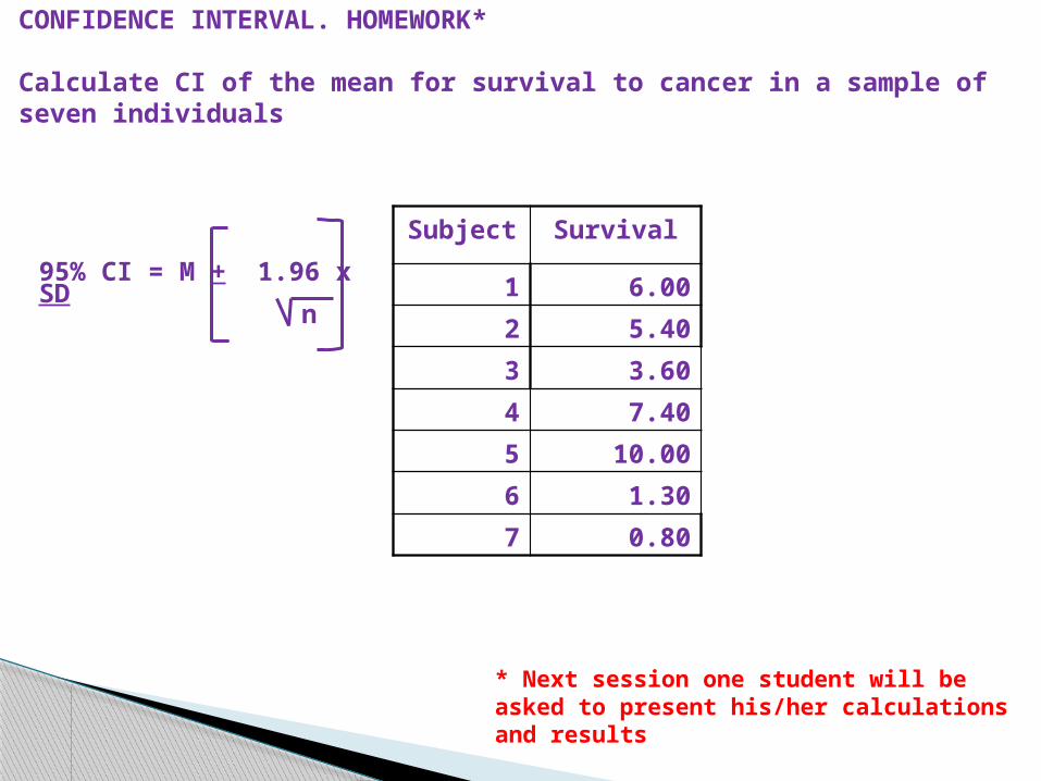
CONFIDENCE INTERVAL. HOMEWORK*
Calculate CI of the mean for survival to cancer in a sample of seven individuals
Subject Survival
1 6.00
2 5.40
3 3.60
4 7.40
5 10.00
6 1.30
7 0.80
n
* Next session one student will be asked to present his/her calculations and results
95% CI = M + 1.96 x SD

Statistical significance
Answers the question: “How sure I’m that my results are not pure chance?”
Commonly used: p = 0.05Interpretation: Up to 5 events (observations) out of 100 could have been produced by chance (and still the value of the estimated parameter - e.g.: effectiveness of a given treatment - would be valid)
Can you work out the interpretation when p is set up at p = 0.001?
INFERENTIAL STATISTICS. STATISTICAL SIGNIFICANCE


![EXPERIMENTAL, QUASI-EXPERIMENTAL, AND …nur.uobasrah.edu.iq/images/pdffolder/Experimental studies 6.pdf · Experimental Design: Experiments (or randomized controlled trials [RCTs])](https://cdn.vdocuments.mx/doc/165x107/5f4c009b337890199f4ada04/experimental-quasi-experimental-and-nur-studies-6pdf-experimental-design.jpg)


