Download - ¯b Cross-Section
Radiation Hard Hybrid Pixel Detectors, and a bb Cross-SectionMeasurement at the CMS Experiment
by
Jennifer A. Sibille
Submitted to the graduate degree program in Physics and the GraduateFaculty of the University of Kansas in partial fulfillment of the
requirements for the degree of Doctor of Philosophy
Committee:
Dr. Alice Bean, Chairperson
Dr. Philip Baringer
Dr. Stephen Sanders
Dr. Kyoungchul Kong
Dr. Cindy Berrie
Dr. Tilman Rohe
Date defended: April 19, 2013
The Dissertation Committee for Jennifer A. Sibille certifies that this is theapproved version of the following dissertation:
Radiation Hard Hybrid Pixel Detectors, and a bb Cross-SectionMeasurement at the CMS Experiment
Committee:
Dr. Alice Bean, Chairperson
Dr. Philip Baringer
Dr. Stephen Sanders
Dr. Kyoungchul Kong
Dr. Cindy Berrie
Dr. Tilman Rohe
Date approved: April 22, 2013
ii
Abstract
Measurements of heavy flavor quark production at hadron colliders provide a
good test of the perturbative quantum chromodynamics (pQCD) theory. It
is also essential to have a good understanding of the heavy quark production
in the search for new physics. Heavy quarks contribute to backgrounds and
signals in measurements of higher mass objects, such as the Higgs boson. A
key component to each of these measurements is good vertex resolution. In
order to ensure reliable operation of the pixel detector, as well as confidence
in the results of analyses utilizing it, it is important to study the effects of
the radiation on the detector.
In the first part of this dissertation, the design of the CMS silicon pixel
detector is described. Emphasis is placed on the effects of the high radi-
ation environment on the detector operation. Measurements of the charge
collection efficiency, interpixel capacitance, and other properties of the pixel
sensors as a function of the radiation damage are presented.
In the second part, a measurement of the inclusive bb production cross section
using the b → µD0X,D0 → Kπ decay chain with data from the CMS experi-
ment at the LHC is presented. The data were recorded with the CMS experi-
ment at the Large Hadron Collider (CERN) in 2010 using unprescaled single
muon triggers corresponding to a total luminosity of 25 pb−1. The differen-
tial cross section is measured for pD0µ
T > 6 GeV/c and |η| < 2.4 correspond-
ing to a total cross section of 4.36±0.54(stat.)+0.28−0.25(sys.)±0.17(B)±0.23(L)
µ b.
iii

Acknowledgements
I can not thank every person who helped me on this journey, but I would like to take this
opportunity to mention a few of those people who were instrumental for this dissertation.
First and foremost I would like to thank Dr. Alice Bean, my advisor, for all of her
help over the years. She has been encouraging and patient through the ups and downs
of my studies, and given me so many opportunities that led me to where I am today. I
would also like to thank Dr. Michael Murray for my first introduction into CERN and
the CMS experiment. In addition I thank Dr. Philip Baringer, Dr. Stephen Sanders,
Dr. K. C. Kong, and Dr. Cindy Berrie for agreeing to serve on my committee.
I am equally grateful to Dr. Tilman Rohe, my supervisor at the Paul Scherrer
Institut (PSI). He spent countless hours with me both in the office and in the lab, and
never tired of answering my questions. My thanks also to Prof. Dr. Roland Horisberger
and the entire CMS Pixel group at PSI, for accepting me into the group as one of their
own.
The work for this PhD was funded by the Marie Curie Initial Training Network
- PArticle Detectors (MC-PAD). I want to thank Dr. Christian Joram and the entire
Marie Curie - Particle Detectors (MC-PAD) Initial Training Network. The opportunites,
connections, and training that I received in this network are what made me into the
scientist I am today. Thank you also to the National Science Foundation, who also
supported this work with the PIRE grant OISE-0730173.
Of course, a huge ”thank you” goes to my family, who have supported me through
all the years of school and hard work that led up to this point, especially my parents,
Mark and Kim Sibille, and my sister, Michelle Sibille, who have never wavered in their
belief in me. A special thanks also goes to my fiance, Thomas Pohlsen, who has been
my sounding board, my cheer leader, and my shoulder to cry on especially in these last
difficult months.
Without all of you, none of this would have been possible.
iv

Contents
1 Introduction 1
2 The LHC and CMS 4
2.1 The Large Hadron Collider . . . . . . . . . . . . . . . . . . . . . . . . . 42.2 The Compact Muon Solenoid Experiment . . . . . . . . . . . . . . . . . 5
2.2.1 The Solenoid . . . . . . . . . . . . . . . . . . . . . . . . . . . . . 62.2.2 The Silicon Tracker . . . . . . . . . . . . . . . . . . . . . . . . . 72.2.3 The Electromagnetic Calorimeter . . . . . . . . . . . . . . . . . . 92.2.4 The Hadronic Calorimeter . . . . . . . . . . . . . . . . . . . . . . 122.2.5 The Muon System . . . . . . . . . . . . . . . . . . . . . . . . . . 142.2.6 The Forward Detectors . . . . . . . . . . . . . . . . . . . . . . . 152.2.7 The Trigger System . . . . . . . . . . . . . . . . . . . . . . . . . 16
3 The CMS Pixel Detector 18
3.1 Detector Layout . . . . . . . . . . . . . . . . . . . . . . . . . . . . . . . 183.2 Read Out and Control System . . . . . . . . . . . . . . . . . . . . . . . 203.3 Modules . . . . . . . . . . . . . . . . . . . . . . . . . . . . . . . . . . . . 21
3.3.1 The Token Bit Manager . . . . . . . . . . . . . . . . . . . . . . . 213.3.2 The Readout Chip . . . . . . . . . . . . . . . . . . . . . . . . . . 233.3.3 The Sensor . . . . . . . . . . . . . . . . . . . . . . . . . . . . . . 29
3.4 Mechanics and Cooling . . . . . . . . . . . . . . . . . . . . . . . . . . . . 303.5 Material Budget . . . . . . . . . . . . . . . . . . . . . . . . . . . . . . . 31
4 Radiation Damage in Silicon Detectors 38
4.1 Basic Properties and Operating Principle of Silicon Sensors . . . . . . . 384.2 Damage Mechanisms . . . . . . . . . . . . . . . . . . . . . . . . . . . . . 40
4.2.1 Surface Damage . . . . . . . . . . . . . . . . . . . . . . . . . . . 404.2.2 Bulk Damage . . . . . . . . . . . . . . . . . . . . . . . . . . . . . 41
4.3 Macroscopic effects . . . . . . . . . . . . . . . . . . . . . . . . . . . . . . 424.3.1 Effective Doping Concentration . . . . . . . . . . . . . . . . . . . 424.3.2 Charge Trapping . . . . . . . . . . . . . . . . . . . . . . . . . . . 444.3.3 Leakage Current . . . . . . . . . . . . . . . . . . . . . . . . . . . 45
4.4 NIEL Scaling . . . . . . . . . . . . . . . . . . . . . . . . . . . . . . . . . 454.5 Annealing . . . . . . . . . . . . . . . . . . . . . . . . . . . . . . . . . . . 464.6 Estimated Requirements for CMS Pixel Detector Sensors . . . . . . . . 47
5 Sensor Measurements 51
5.1 Charge Collection Efficiency . . . . . . . . . . . . . . . . . . . . . . . . . 535.1.1 Testing Setup and Procedure . . . . . . . . . . . . . . . . . . . . 535.1.2 Analysis . . . . . . . . . . . . . . . . . . . . . . . . . . . . . . . . 545.1.3 Results . . . . . . . . . . . . . . . . . . . . . . . . . . . . . . . . 56
5.2 Detection Efficiency . . . . . . . . . . . . . . . . . . . . . . . . . . . . . 655.2.1 Test Beam . . . . . . . . . . . . . . . . . . . . . . . . . . . . . . 655.2.2 Lab Setup . . . . . . . . . . . . . . . . . . . . . . . . . . . . . . . 72
v
5.3 Interpixel Capacitance . . . . . . . . . . . . . . . . . . . . . . . . . . . . 735.3.1 Measurements . . . . . . . . . . . . . . . . . . . . . . . . . . . . 765.3.2 Simulations . . . . . . . . . . . . . . . . . . . . . . . . . . . . . . 83
5.4 High Voltage Tests on Single Sided Sensors . . . . . . . . . . . . . . . . 86
6 b Production 93
6.1 Theory . . . . . . . . . . . . . . . . . . . . . . . . . . . . . . . . . . . . . 936.2 Monte Carlo Event Generators . . . . . . . . . . . . . . . . . . . . . . . 936.3 Other Measurements . . . . . . . . . . . . . . . . . . . . . . . . . . . . . 95
6.3.1 CDF measurement of b hadron production cross section . . . . . 966.3.2 LHCb . . . . . . . . . . . . . . . . . . . . . . . . . . . . . . . . . 976.3.3 ATLAS . . . . . . . . . . . . . . . . . . . . . . . . . . . . . . . . 986.3.4 CMS . . . . . . . . . . . . . . . . . . . . . . . . . . . . . . . . . . 100
6.4 Summary . . . . . . . . . . . . . . . . . . . . . . . . . . . . . . . . . . . 102
7 bb Cross Section Measurement 104
7.1 Introduction . . . . . . . . . . . . . . . . . . . . . . . . . . . . . . . . . . 1047.2 Data and Monte Carlo Samples . . . . . . . . . . . . . . . . . . . . . . . 1047.3 Event Selection . . . . . . . . . . . . . . . . . . . . . . . . . . . . . . . . 105
7.3.1 Acceptance and Quality Cuts . . . . . . . . . . . . . . . . . . . . 1087.3.2 Selection Cut Variables . . . . . . . . . . . . . . . . . . . . . . . 1127.3.3 Cut Optimization . . . . . . . . . . . . . . . . . . . . . . . . . . 115
7.4 Efficiencies . . . . . . . . . . . . . . . . . . . . . . . . . . . . . . . . . . 1247.4.1 Trigger Efficiency . . . . . . . . . . . . . . . . . . . . . . . . . . . 126
7.5 D0 Mass Fits . . . . . . . . . . . . . . . . . . . . . . . . . . . . . . . . . 1387.5.1 Wrong Charge Correlation Distributions . . . . . . . . . . . . . . 146
7.6 Systematic Uncertainties . . . . . . . . . . . . . . . . . . . . . . . . . . . 1487.7 Results . . . . . . . . . . . . . . . . . . . . . . . . . . . . . . . . . . . . . 157
8 Conclusion 164
A Hardness Factors 179
B Single Chip Samples 179
C Single ROC DAC values 182
D Backgrounds 183
D.1 Right Sign Charge Correlation . . . . . . . . . . . . . . . . . . . . . . . 184D.2 Wrong Sign Charge Correlation . . . . . . . . . . . . . . . . . . . . . . . 191
E Alternate Cut Optimization 198
F µ Bins 201
F.1 Reconstruction and Selection Efficiency . . . . . . . . . . . . . . . . . . 201F.2 D0 Candidate Invariant Mass Fits . . . . . . . . . . . . . . . . . . . . . 201F.3 Wrong Charge Correlation Distributions . . . . . . . . . . . . . . . . . . 211
vi

F.4 Systematic Uncertainties . . . . . . . . . . . . . . . . . . . . . . . . . . . 211F.5 Results . . . . . . . . . . . . . . . . . . . . . . . . . . . . . . . . . . . . . 212
vii
List of Tables
1 Single ROC samples used in the charge collection efficiency and detectionefficiency measurements. . . . . . . . . . . . . . . . . . . . . . . . . . . . 52
2 Samples used in the interpixel capacitance measurements and the mea-sured capacitance at a bias voltage of 150 V. Errors are discussed in thetext. . . . . . . . . . . . . . . . . . . . . . . . . . . . . . . . . . . . . . . 80
3 2010 Data samples used for the analysis. . . . . . . . . . . . . . . . . . . 1054 Variables used for acceptance and quality cuts and their cut values. The
Signal Eff and BG MC Eff columns show the efficiencies of the truthmatched signal and background events, respectively, after each cut. . . . 112
5 Selection cut efficiencies in bins of pT(µD0) using Monte Carlo eventswith pT(µ) > 5 GeV and |η(µ)| < 2.4. . . . . . . . . . . . . . . . . . . 122
6 Selection cut efficiencies in bins of pT(µD0) using Monte Carlo eventswith pT(µ) > 15 GeV and |η(µ)| < 2.4. . . . . . . . . . . . . . . . . . . . 123
7 The reconstruction and selection efficiency (εrec · εcut) in each pT (µD0)and |η(µD0)| bin. The Eff5 column is using Monte Carlo events with pT(µ) > 5 GeV, and the Eff15 column is using Monte Carlo events with pT(µ) > 15 GeV. In both cases |η(µ)| < 2.4 is required. . . . . . . . . . . . 126
8 2010 Data samples used for the trigger efficiency calculation. . . . . . . 1279 The number of D0 candidates in each dataset before and after the trigger
efficiency weighting, as well as the ratio of unweighted to weighted data.All datasets have at least pT (µ) > 6 GeV/c, pT(K,π) > 0.5 GeV/c, and|η(µ,K,π)| < 2.4. The uncertainty is the uncertainty from the fit. . . . 139
10 The number of D0 candidates in each bin. For the 2010A and 2010Bcolumns, the numbers are the results from the invariant mass fits in RunA and Run B data, respectively. For the MC columns they are the numberof tagged signal events in the Monte Carlo. All columns have at least pT(µ) > 6 GeV and |η(µ)| < 2.4. The uncertainty is the uncertainty fromthe fit. . . . . . . . . . . . . . . . . . . . . . . . . . . . . . . . . . . . . . 145
11 The number of D0 candidates found by the fit assuming a signal for thewrong charge correlation for pT (µ) > 6 GeV/c and |η(µ)| < 2.4. . . . . 147
12 Systematic uncertainty due to the error on the trigger efficiency in eachpT (µD0) bin. The Run A data uses the HLT Mu5 trigger, and the RunB data uses the HLT Mu15 v1 trigger. . . . . . . . . . . . . . . . . . . . 151
13 Systematic uncertainty due to the error on the trigger efficiency in each|η(µD0)| bin. The Run A data uses the HLT Mu5 trigger, and the RunB data uses the HLT Mu15 v1 trigger. . . . . . . . . . . . . . . . . . . . 152
14 Systematic uncertainty due to the statistical error on the selection effi-ciency for Run A with pT (µ) > 6 GeV/c and |η(µ)| < 2.4. . . . . . . . . 153
15 Systematic uncertainty due to the statistical error on the selection effi-ciency for Run B with pT (µ) > 16 GeV/c and |η(µ)| < 2.4. . . . . . . . 153
16 The number of D0 candidates found when varying the cut on xb by 0.05for Monte Carlo with pT (µ) > 6 GeV/c. The last column, labeled ”Stat.Uncert.”, shows the statistical uncertainty as a comparison. . . . . . . . 154
viii
17 The number of D0 candidates found when varying the cut on xb by 0.05for Monte Carlo with pT (µ) > 16 GeV/c. The last column, labeled”Stat. Uncert.”, shows the statistical uncertainty as a comparison. . . . 155
18 Systematic uncertainties on the cross section. . . . . . . . . . . . . . . . 15619 The cross section in each pT (µD0) bin. . . . . . . . . . . . . . . . . . . 16220 The cross section in each |η(µD0)| bin. . . . . . . . . . . . . . . . . . . . 16321 Hardness factors of irradiation facilities used in this work [1]. . . . . . . 17922 Complete table of single ROC samples used in the charge collection effi-
ciency and detection efficiency measurements. . . . . . . . . . . . . . . . 17923 Commonly used DAC values used for testing CMS barrel pixel sensors. . 18224 Background classifications. . . . . . . . . . . . . . . . . . . . . . . . . . . 18325 Selection cut efficiencies in bins of pT(µ) using the HLT Mu5 trigger. . . 20126 Selection cut efficiencies in bins of pT(µ) using the HLT Mu15 v1 trigger. 20127 The reconstruction and selection efficiency in each pT (µ) and |η(µ)| bin. 20228 Systematic uncertainty due to the error on the trigger efficiency in each
bin. . . . . . . . . . . . . . . . . . . . . . . . . . . . . . . . . . . . . . . 21429 Systematic uncertainty due to the error on the trigger efficiency in each
|η(µ)| bin. . . . . . . . . . . . . . . . . . . . . . . . . . . . . . . . . . . . 21530 Systematic uncertainty due to the error on the selection efficiency for
Run A. . . . . . . . . . . . . . . . . . . . . . . . . . . . . . . . . . . . . 21631 Systematic uncertainty due to the error on the selection efficiency for
Run B. . . . . . . . . . . . . . . . . . . . . . . . . . . . . . . . . . . . . . 21632 The cross section in each pT (µ) bin. . . . . . . . . . . . . . . . . . . . . 21833 The cross section in each |η(µ)| bin. . . . . . . . . . . . . . . . . . . . . 219
ix

List of Figures
1 The LHC accelerator complex, showing the locations of the 4 experi-ments [2]. . . . . . . . . . . . . . . . . . . . . . . . . . . . . . . . . . . . 5
2 The CMS Detector [3]. . . . . . . . . . . . . . . . . . . . . . . . . . . . . 63 Layout of the tracker, showing the pixel detector, TIB, TID, TOB, and
TEC [3]. . . . . . . . . . . . . . . . . . . . . . . . . . . . . . . . . . . . . 84 Number of measurement points in the strip tracker as a function of pseu-
dorapidity . Filled circles show the total number (back-to-back modulescount as one) while open squares show the number of stereo layers [3]. . 9
5 Primary vertex resolution in x (a), y (b), and z (c) as a function of thenumber of tracks [4]. . . . . . . . . . . . . . . . . . . . . . . . . . . . . . 10
6 Track transverse (left) and longitudinal (right) impact parameter resolu-tion as a function of the track pT [4]. . . . . . . . . . . . . . . . . . . . 11
7 Track transverse (left) and longitudinal (right) impact parameter resolu-tion as a function of η of the track for different values of the track pT[4]. . . . . . . . . . . . . . . . . . . . . . . . . . . . . . . . . . . . . . . . 12
8 Layout of the ECAL including the barrel, endcaps, and preshower. . . . 139 Longitudinal view of the CMS detector showing the positions of the
hadron barrel (HB), endcap (HE), outer (HO) and forward (HF) calorime-ters. . . . . . . . . . . . . . . . . . . . . . . . . . . . . . . . . . . . . . . 14
10 Side cutaway view of CASTOR showing the EM and HAD sections. . . 1611 Side cutaway view of the ZDC showing the EM and HAD sections. . . . 1712 The geometrical layout of one quadrant of the CMS pixel detector, show-
ing the locations of the three barrel layers and two forward disks. [3] . . 1913 One half disk of the supporting structure of the FPix, showing the tilted
blades [5]. . . . . . . . . . . . . . . . . . . . . . . . . . . . . . . . . . . . 2014 Diagram of the pixel detector read out chain and control system. More
details can be found in [3]. . . . . . . . . . . . . . . . . . . . . . . . . . . 2115 Picture of a BPix half module (left) and full module (right). The center
shows an exploded view of a module, with the different components labeled. 2216 A read out of a full module with a hit in ROC 0, showing the TBM
header, hit information from ROC 0, headers from the remaining ROCs,and TBM trailer. . . . . . . . . . . . . . . . . . . . . . . . . . . . . . . . 23
17 The read out chip. . . . . . . . . . . . . . . . . . . . . . . . . . . . . . . 2418 Schematic of the pixel unit cell. . . . . . . . . . . . . . . . . . . . . . . . 2619 The pixel address encoding levels. . . . . . . . . . . . . . . . . . . . . . . 2720 A read out of a hit from a ROC. . . . . . . . . . . . . . . . . . . . . . . 2821 Sketch showing a charged particle crossing the silicon sensor. The n+
pixel implants collect the electrons. [6] . . . . . . . . . . . . . . . . . . . 3222 The Lorentz angle for the sensors in a 4 T magnetic field as a function
of bias voltage [7]. . . . . . . . . . . . . . . . . . . . . . . . . . . . . . . 3323 Picture of four pixels in the same double column for the FPix. The pixels
have a pitch of 100 x 150 µm. [3] . . . . . . . . . . . . . . . . . . . . . . 34
x

24 Picture of four pixels in the BPix. The pixels have a pitch of 100 x150 µm. The indium bumps have been deposited but not reflown, andare visible. [3] . . . . . . . . . . . . . . . . . . . . . . . . . . . . . . . . . 35
25 Drawing of one of the supply tubes. [3] . . . . . . . . . . . . . . . . . . . 3626 A sketch of one half cylinder of the barrel pixels. [3] . . . . . . . . . . . 3627 Left: Material budget for the whole CMS tracker, showing the various
subdetector contributions. Right: Material budget for the pixel barreldetector, showing the various categories of material. [8] . . . . . . . . . . 37
28 Formation of the space charge region around the pn-junction. The filledcircles are free electrons, and the open circles are free holes. . . . . . . . 39
29 Simulation of the path of a primary knock-on atom through the silicon.Point defects are shown in red and cluster defects are shown in blue [9]. 42
30 Change in the effective doping concentration as well as the voltage re-quired for full depletion as a function of the fluence [1]. . . . . . . . . . 44
31 Illustration of the double peak effect. The p+-contact is at x = 0, and then+-contact is at x = d. (a) Electric field in an unirradiated detector. (b)Thermally generated current, with the electron (red) and hole (green)currents. (c) Space charge distribution in an irradiated detector. (d)Electric field in an irradiated detector. Figure reproduced from [10]. . . 49
32 Change in effective doping concentration as a function of annealing time,taken from [1]. . . . . . . . . . . . . . . . . . . . . . . . . . . . . . . . . 50
33 Single sensor testing setup. . . . . . . . . . . . . . . . . . . . . . . . . . 5534 Charge distribution for different cluster sizes. . . . . . . . . . . . . . . . 5735 Charge distribution for an unirradiated sample with a bias voltage of -150
V fit by a LanGau function. . . . . . . . . . . . . . . . . . . . . . . . . . 5836 Charge vs bias voltage for an unirradiated sample. . . . . . . . . . . . . 5937 Collected charge vs bias voltage for all tested samples. . . . . . . . . . . 6038 Two dimensional map of hits within the sample irradiated to 5×10¹⁵ neq/cm2.
The distinctive “bulls-eye” pattern of a point source is clearly visible, in-dicating that the signals are produced by actual particles and not noise. 61
39 Cluster size for unirradiated sensors. . . . . . . . . . . . . . . . . . . . . 6240 Cluster size for sensors irradiated to a fluence of 5× 10¹⁵ neq/cm2 . . . . 6341 Collected charge vs fluence for all tested samples. . . . . . . . . . . . . . 6442 Top: Diagram of the pixel telescope used at the testbeam, showing the
location of the device under test. Bottom: Photograph of the pixel tele-scope. . . . . . . . . . . . . . . . . . . . . . . . . . . . . . . . . . . . . . 67
43 Photograph of the trigger board. The sensor is under the foil cap. . . . 6844 An example beam event. The small white spots correspond to the hit
position. The four maps on the left are the telescope sensors, while themap on the right is the device under test. . . . . . . . . . . . . . . . . . 69
45 Correlation plot between the hit column in two telescope sensors. Thecorrelated hits, corresponding to particles passing through the telescope,are seen in the dark line along the diagonal. The scattered off-diagonalpoints correspond to noise hits in one or both of the telescope sensors. . 70
xi

46 Illustration of timewalk. Low amplitude signals cross threshold late andare assigned to the wrong bunch crossing. . . . . . . . . . . . . . . . . . 71
47 Diagram of modified CCE testing setup. The source is placed above thesample, and the scintillator and photomultiplier tube are placed belowthe sample. . . . . . . . . . . . . . . . . . . . . . . . . . . . . . . . . . . 73
48 Photograph of the modified CCE testing setup and trigger electronics. . 7449 Diagram showing how the source position affects the efficiency. Different
source positions provide different paths for the scattered particles. . . . 7550 Picture of part of the readout replacement chip. The basic cell of one
pixel in the center (blue), surrounded by the eight neighboring pixels(red), is highlighted. . . . . . . . . . . . . . . . . . . . . . . . . . . . . . 77
51 The interpixel capacitance measurement setup. . . . . . . . . . . . . . . 7852 Diagram of interpixel capacitance. C0 represents the capacitance between
pixels through the bulk, C1 represents the capacitance between the pixelimplant and the p-spray, and R represents the resistance of the p-spray. 79
53 Interpixel capacitance vs. bias voltage before irradiation. . . . . . . . . . 8254 Results of the interpixel capacitance measurements. . . . . . . . . . . . 8355 The geometry and doping profile of the simulated sensor area. . . . . . . 8456 The current induced in the gate as a function of bias voltage in the
simulation for different gap sizes. . . . . . . . . . . . . . . . . . . . . . . 8657 Diagram of single sided sensor showing the potential for sparking between
the sensor and ROC. . . . . . . . . . . . . . . . . . . . . . . . . . . . . . 8758 Damage to sensor from high voltage sparking. The ground pad of the
ROC is completely destroyed. Damage to the aluminum on the back ofthe sensor is also visible in the bottom of the picture. . . . . . . . . . . 88
59 Damage to neighboring pads on the ROC from high voltage sparking. . 8860 Photograph of sparks between ROC and sensor. . . . . . . . . . . . . . . 8961 Diagram of single sided sensor using glue to fill the edge gap between the
sensor and the ROC. . . . . . . . . . . . . . . . . . . . . . . . . . . . . . 9062 Damage to sensors with glue filled gaps. . . . . . . . . . . . . . . . . . . 9163 Diagram of the proposed solution to protect wire bond pads during Pary-
lene deposition. . . . . . . . . . . . . . . . . . . . . . . . . . . . . . . . . 9264 Examples of the LO and NLO processes for heavy quark production at
hadron colliders. [11] . . . . . . . . . . . . . . . . . . . . . . . . . . . . . 9465 Topology of B hadron event. . . . . . . . . . . . . . . . . . . . . . . . . . 9566 The unfolded b hadron differential cross section in pp collisions for the
CDF measurements at√s = 1.96 TeV of Hb → µD0X and Hb → µD∗X
for pT (Hb) > 9 GeV/c and |y(Hb)| < 0.6 compared with predictions fromFONLL theory [12]. . . . . . . . . . . . . . . . . . . . . . . . . . . . . . 97
xii

67 LHCb measurement of σ(pp → HbX) as a function of η(µD0) [13] forthe microbias (×) and triggered (•) samples, shown displaced from thebin center and the average (+). In both data sets, pT (K,π) > 300 MeVis required. The muon pT is required to be at least 500 MeV for themicrobias dataset and at least 1.3 GeV for the triggered dataset. Thedata are shown as points with error bars, the MCFM prediction as adashed line, and the FONLL prediction as a thick solid line. The thinupper and lower lines indicate the theoretical uncertainties on the FONLLprediction. The systematic uncertainties in the data are not included. . 99
68 ATLAS measurement of σ(pp → HbX) unfolded and as a function ofpT (Hb) (left) and |η(Hb)| (right) for pT (Hb) > 9 GeV/c and |η(Hb)| <2.5, compared with theoretical predictions. The inner error bars are thestatistical uncertainties, and the outer error bars are the statistical plustotal systematic uncertainties [14]. . . . . . . . . . . . . . . . . . . . . . 100
69 CMS measurement of σ(bb → µX) for pT (µ) > 6 GeV/c and |η(µ)| < 2.1,as a function of pT (left) and |η| (right), compared with theoretical predic-tions. The PYTHIA predictions, shown in green, overestimate the crosssection, while the MC@NLO predictions, shown in red, underestimatethe cross section [6]. . . . . . . . . . . . . . . . . . . . . . . . . . . . . . 101
70 Comparison of the bb → µX cross section as a function of muon pT forvarious Monte Carlo event generators with the expected cross section forFONLL. The CMS data are also superimposed [15]. . . . . . . . . . . . 102
71 Example of a B → µD0X decay. The B travels from the primary vertex(PV) shown by the dotted line then decays at the black circle shown. . . 106
72 D0 candidate invariant mass distribution before cuts showing differentsources of background in Monte Carlo. . . . . . . . . . . . . . . . . . . . 107
73 Distributions of pT (left) and η (right) for tracks identified as tight muonsshown after the track quality cuts for Monte Carlo events (filled his-togram) and 2010A data events (points). The Monte Carlo is normalizedto the Run A luminosity. . . . . . . . . . . . . . . . . . . . . . . . . . . . 109
74 Distributions of pT (left) and η (right) for kaon/pion tracks shown af-ter the track quality cuts for Monte Carlo events (filled histogram) and2010A data events (points). The Monte Carlo is normalized to the runA luminosity. . . . . . . . . . . . . . . . . . . . . . . . . . . . . . . . . . 109
75 Distributions of ∆R(µ,K) (left) and ∆R(µ,π) (right) after skim cuts fortagged signal (red) and background (black) Monte Carlo events. Thedistributions are normalized to unit area. . . . . . . . . . . . . . . . . . 110
76 The K−π+ invariant mass distribution for the 2010A dataset (left) and2010B dataset (right) after the acceptance and quality cuts. . . . . . . . 110
77 The K−π+ invariant mass distribution for tagged signal (red) and back-ground (black) Monte Carlo events after the acceptance and quality cuts.The distributions are normalized to unit area. . . . . . . . . . . . . . . . 111
78 The µD0 invariant mass distribution for tagged signal (red) and back-ground (black) Monte Carlo events after the acceptance cuts. The dis-tributions are normalized to unit area. . . . . . . . . . . . . . . . . . . . 111
xiii

79 Definition of the distance of closest approach (doca). . . . . . . . . . . . 11380 Distributions of the D0 (left) and b-hadron (right) candidate doca (right)
after all other selection cuts for tagged signal (red) and background(black) Monte Carlo events. The distributions are normalized to unitarea. . . . . . . . . . . . . . . . . . . . . . . . . . . . . . . . . . . . . . . 114
81 Distribution of 3D flight distance significance for the D0 (left) and b-hadron (right) candidates after the acceptance cuts for tagged signalMonte Carlo events (red) and tagged background MC events (black).The distributions are normalized to unit area. . . . . . . . . . . . . . . . 115
82 Definition of the muon signed transverse impact parameter. . . . . . . . 11683 Distribution of muon signed impact parameter shown after the acceptance
cuts for tagged signal Monte Carlo events (red) and tagged backgroundMC events (black). The distributions are normalized to unit area. . . . 117
84 Distributions of xb after all acceptance cuts for tagged signal Monte Carloevents (red) and background MC events (black). The distributions arenormalized to unit area. . . . . . . . . . . . . . . . . . . . . . . . . . . . 117
85 Distributions of xb for Monte Carlo events (red), Monte Carlo events withpT(µ) > 15 GeV/c (purple), Run A data events (black), and Run B dataevents (blue). The distributions are normalized to unit area. . . . . . . . 118
86 Diagram of the pointing angle. . . . . . . . . . . . . . . . . . . . . . . . 11987 Distributions of the b-hadron (left) and D0 (right) candidate pointing
angle after the acceptance cuts for tagged signal (red) and background(black) Monte Carlo events. The distributions are normalized to unit area.120
88 Distributions of S/√B after the quality cuts. . . . . . . . . . . . . . . . 120
89 Distributions of S/√B after the quality cuts, and xb > 0.7. . . . . . . . 121
90 Distributions of S/√B after the acceptance cuts, xb > 0.7, and B doca
< 0.007. . . . . . . . . . . . . . . . . . . . . . . . . . . . . . . . . . . . . 12191 Distribution of S/
√B for the muon transverse impact parameter after
the acceptance cuts, xb > 0.7, B doca < 0.007, and D0 doca < 0.015. . . 12292 D0 mass distributions in bins of pT (µD0 ) (GeV/c) for Monte Carlo
events with |η(µ,K,π)| < 2.4, pT(µ) > 6 GeV/c, and pT(K,π) > 0.5GeV/c. The distributions are fit with a linear background plus a doubleGaussian signal. . . . . . . . . . . . . . . . . . . . . . . . . . . . . . . . . 128
93 D0 mass distributions in bins of pT (µD0 ) (GeV/c) for Monte Carloevents with pT (µ) > 16 GeV/c, pT(K,π) > 0.5 GeV/c, and |η(µ,K,π)| <2.4. The distributions are fit with a linear background plus a doubleGaussian signal. . . . . . . . . . . . . . . . . . . . . . . . . . . . . . . . . 129
94 D0 mass distributions in bins of |η(µD0)| for Monte Carlo events withpT (µ) > 6 GeV/c and pT(K,π) > 0.5 GeV/c. The distributions are fitwith a linear background plus a double Gaussian signal. . . . . . . . . . 130
95 D0 mass distributions in bins of |η(µD0)| for Monte Carlo events withpT (µ) > 16 GeV/c and pT(K,π) > 0.5 GeV/c. The distributions are fitwith a linear background plus a double Gaussian signal. . . . . . . . . . 131
96 The tracking, reconstruction, and event selection efficiency (εrec · εcut) forRun A (left) and Run B (right) as a function of pT (µD0) with |η(µ)| < 2.4.131
xiv

97 The tracking, reconstruction, and event selection efficiency (εrec · εcut)for Run A (left) and Run B (right) as a function of |η(µD0)| with pT(µD0) > 6 GeV/c for Run A and pT (µD0) > 16 GeV/c for Run B. . . . 132
98 The tracking, reconstruction, and event selection efficiency (εrec · εcut) forRun A (left) and Run B (right) as a function of pT (µD0) with |η(µ)| < 2.4.132
99 The tracking, reconstruction, and event selection efficiency (εrec · εcut) forRun A (left) and Run B (right) as a function of |η(µD0)| with pT (µ) > 6GeV/c. . . . . . . . . . . . . . . . . . . . . . . . . . . . . . . . . . . . . 133
100 HLT Mu5 trigger efficiency in bins of pT (µ) (GeV/c) . . . . . . . . . . 134101 HLT Mu5 trigger efficiency in bins of |η(µ)| . . . . . . . . . . . . . . . . 135102 HLT Mu15 v1 trigger efficiency in bins of pT (µ) (GeV/c) . . . . . . . . 136103 HLT Mu15 v1 trigger efficiency in bins of |η(µ)| . . . . . . . . . . . . . . 137104 The Kπ invariant mass distribution before and after the trigger efficiency
weighting for Run A (left) and Run B (right). . . . . . . . . . . . . . . . 137105 Kπ invariant mass distribution for pT(K,π) > 0.5 GeV/c, and |η(µ,K,π)| <
2.4, pT (µ) > 6 GeV/c for Run A and Monte Carlo (left), and with pT(µ) > 16 GeV/c for Run B and Monte Carlo (right). The data eventsare weighted by the trigger efficiency. The Monte Carlo is scaled to theluminosity of the data. . . . . . . . . . . . . . . . . . . . . . . . . . . . . 138
106 D0 mass distribution for pT (µ) > 6 GeV/c for Run A (left), pT (µ) > 16GeV/c for Run B (right), pT(K,π) > 0.5 GeV/c, and |η(µ,K,π)| < 2.4,before weighting the data events by the trigger efficiency. . . . . . . . . 139
107 D0 mass distribution for pT (µ) > 6 GeV/c for Run A (left), pT (µ) > 16GeV/c for Run B (right), pT(K,π) > 0.5 GeV/c, and |η(µ,K,π)| < 2.4,after weighting the data events by the trigger efficiency. . . . . . . . . . 140
108 D0 mass distributions in bins of pT (GeV/c) for the 2010A datasetwith pT (µ) > 6 GeV/c, pT(K,π) > 0.5 GeV/c and |η(µ,K,π)| < 2.4,weighted by the trigger efficiency. . . . . . . . . . . . . . . . . . . . . . . 141
109 D0 mass distributions in bins of pT (GeV/c) for the 2010B dataset with pT(µ) > 16 GeV/c, pT(K,π) > 0.5 GeV/c and |η(µ,K,π)| < 2.4, weightedby the trigger efficiency. . . . . . . . . . . . . . . . . . . . . . . . . . . . 142
110 D0 mass distributions in bins of |η| for the 2010A dataset with pT (µ) > 6GeV/c and pT(K,π) > 0.5 GeV/c, weighted by the trigger efficiency. . . 143
111 D0 mass distributions in bins of |η| for the 2010B dataset with pT (µ) > 16GeV/c and pT(K,π) > 0.5 GeV/c, weighted by the trigger efficiency. . . 144
112 D0 mass distribution of the wrong charge correlation candidates for pT(µ) > 6 GeV/c, pT(K,π) > 0.5 GeV/c, and |η(µ,K,π)| < 2.4 for the2010A data (top left), 2010B data (top right), and Monte Carlo events(bottom). Fits assume a Gaussian signal plus a linear background. . . . 146
113 D0 mass distribution of the wrong charge correlation candidates for pT(µ) > 6 GeV/c, pT(K,π) > 0.5 GeV/c, and |η(µ,K,π)| < 2.4 for the2010A data (top left), 2010B data (top right), and Monte Carlo events(bottom). Fits assume background only. . . . . . . . . . . . . . . . . . . 147
xv
114 Cross section as a function of pT(µD0) for Run A (black), Run B (blue),and Monte Carlo (red) events with |η(µ)| < 2.4. Error bars show the sta-tistical uncertainty, and the colored bands show the combined statisticaland systematic uncertainty. . . . . . . . . . . . . . . . . . . . . . . . . . 159
115 Cross section as a function of |η|(µD0) for Run A (black) and Monte Carlo(red) events with pT (µ) > 6 GeV/c. Error bars show the statisticaluncertainty, and the colored bands show the combined statistical andsystematic uncertainty. . . . . . . . . . . . . . . . . . . . . . . . . . . . . 160
116 Cross section as a function of |η|(µD0) for Run B (blue) and Monte Carlo(red) events with pT (µ) > 16 GeV/c. Error bars show the statisticaluncertainty, and the colored bands show the combined statistical andsystematic uncertainty. . . . . . . . . . . . . . . . . . . . . . . . . . . . . 161
117 After acceptance cuts only. . . . . . . . . . . . . . . . . . . . . . . . . . 184118 After xb cut. . . . . . . . . . . . . . . . . . . . . . . . . . . . . . . . . . 185119 After D0 pointing angle cut. . . . . . . . . . . . . . . . . . . . . . . . . . 186120 After B pointing angle cut. . . . . . . . . . . . . . . . . . . . . . . . . . 187121 After D0 doca cut. . . . . . . . . . . . . . . . . . . . . . . . . . . . . . . 188122 After B 3D flight sig cut. . . . . . . . . . . . . . . . . . . . . . . . . . . 189123 After B doca cut. (all selection cuts) . . . . . . . . . . . . . . . . . . . . 190124 After acceptance cuts only. . . . . . . . . . . . . . . . . . . . . . . . . . 191125 After xb cut. . . . . . . . . . . . . . . . . . . . . . . . . . . . . . . . . . 192126 After D0 pointing angle cut. . . . . . . . . . . . . . . . . . . . . . . . . . 193127 After B pointing angle cut. . . . . . . . . . . . . . . . . . . . . . . . . . 194128 After D0 doca cut. . . . . . . . . . . . . . . . . . . . . . . . . . . . . . . 195129 After B 3D flight sig cut. . . . . . . . . . . . . . . . . . . . . . . . . . . 196130 After B doca cut. (all selection cuts) . . . . . . . . . . . . . . . . . . . . 197131 Distributions of S/
√B after the quality cuts. . . . . . . . . . . . . . . . 198
132 Distributions of S/√B after the quality cuts, and B doca > 0.007. . . . 199
133 Distributions of S/√B after the acceptance cuts, B > 0.007, and D0
doca < 0.015. . . . . . . . . . . . . . . . . . . . . . . . . . . . . . . . . . 200134 D0 mass distributions in bins of pT (GeV/c) for Monte Carlo events. . . 203135 D0 mass distributions in bins of |η| for Monte Carlo events. . . . . . . . 204136 D0 mass distributions in bins of |η| for Monte Carlo events with pT (µ)
> 15GeV. . . . . . . . . . . . . . . . . . . . . . . . . . . . . . . . . . . . 205137 The tracking, reconstruction and event selection efficiency as a function
of pT (µ). . . . . . . . . . . . . . . . . . . . . . . . . . . . . . . . . . . . 206138 The tracking, reconstruction, and event selection efficiency for Run A
(left) and Run B (right) as a function of |η(µ)|. . . . . . . . . . . . . . . 206139 D0 mass distributions in bins of pT (GeV/c) for the 2010A dataset. . . . 207140 D0 mass distributions in bins of pT (GeV/c) for the 2010B dataset. . . . 208141 D0 mass distributions in bins of |η| for the 2010A dataset. . . . . . . . . 209142 D0 mass distributions in bins of |η| for the 2010B dataset. . . . . . . . . 210143 D0 mass distribution of the wrong charge correlation candidates for the
whole pT and η range for the 2010A data (top left), 2010B data (topright), and Monte Carlo events (bottom). . . . . . . . . . . . . . . . . . 211
xvi
144 D0 mass distribution of the wrong charge correlation candidates for thewhole pT and η range for the 2010A data (top left), 2010B data (topright), and Monte Carlo events (bottom). Fits assume background only. 212
145 Cross section as a function of pT(µ) for Run A (black), Run B (blue), andMonte Carlo (red) events. Error bars show the statistical uncertainty, andthe colored bands show the combined statistical and systematic uncertainty.213
146 Cross section as a function of |η|(µ) for Run A (black) and Monte Carlo(red) events. Error bars show the statistical uncertainty, and the coloredband shows the combined statistical and systematic uncertainty. . . . . 213
147 Cross section as a function of |η|(µ) for Run B (blue) and Monte Carlo(red) events. Error bars show the statistical uncertainty, and the coloredband shows the combined statistical and systematic uncertainty. . . . . 217
xvii
1 Introduction
The Standard Model (SM) of particle physics attempts to describe the structure of
matter and the interactions between the elementary particles and forces which make up
the universe. In 1961, Sheldon Glashow suggested a unification of the electromagnetic
and weak forces [16]. The addition of the Higgs mechanism by Steven Weinberg and
Abdus Salam in the late 1960’s completed the current version of the theory [17, 18].
Since then, the Standard Model has done a remarkably good job of describing a large
number of experimental results, as well as correctly predicting the existence of several
particles before they were experimentally observed (c [19, 20, 21], b [22, 23], t [24, 25, 26],
ντ [27, 28], W/Z bosons, gluon [29]).
In the SM there are 12 spin-12 fermions and 4 spin-1 gauge bosons. The bosons act
as the carriers of the forces. The SM incorporates three of the four fundamental forces:
the electromagnetic, the weak, and the strong force. Gravity, which is only relevant at
macroscopic distances, is not included in the theory.
The 12 fermions are divided into the 6 quarks (u, d, s, c, b, t) and the 6 leptons
(e, µ, τ, νe, νµ, ντ ). They are further divided into 3 generations, and have a wide range
in masses. The lighest quarks (u, d) have a mass on the order of a few MeV, while the t
has a mass of about 172 GeV. Each of the particles also has a charge-conjugate partner,
called its “anti-particle.”
The b quark is one of the third-generation quarks, together with the t (or top) quark.
The b has a bare mass around 4 GeV/c2 and a charge of −13e. It was first predicted in
1972 by Kobayashi and Maskawa to explain CP-violation, and was discovered in 1977
at Fermilab [22, 23]. The b-quark decays via the weak interaction to a u or c quark,
but the decay is suppressed by the CKM matrix. It is the heaviest quark which can
hadronize, with a mean lifetime of approximately 10−12s.
Heavy flavor physics is described theoretically by perturbative Quantum Chromody-
namics (pQCD). The b production cross section at the LHC is very large, which makes
1

it a perfect opportunity to study how well the theory describes the strong interaction.
In addition, b-quarks make up a large background to many other measurements which
will be performed at the LHC. As such, the production mechanisms should be well
understood.
Despite the many successes of the Standard Model, it is still incomplete. The search
for the Higgs boson was one of the main motivations for the Large Hadron Collider
(LHC). Recently, the ATLAS and CMS experiments at the LHC have published the
discovery of a new boson with a mass of approximately 125 GeV, which is so far con-
sistent with the Higgs boson [30, 31]. In addition, the Standard Model offers no expla-
nation for the nature of dark matter, or for the matter-antimatter asymmetry. Many
additional theories, such as Supersymmetry, have been developed in attempts to answer
these questions. Many of these theories predict effects which should manifest at the
LHC.
In hadron collider experiments the collisions produce very dense events. The track-
ing detector is essential in order to reconstruct the interesting events. Strip and pixel
detectors provide the necessary granularity and resolution to reliably reconstruct ver-
tices. Due to the long lifetime of b mesons, they are able to travel distances on the order
of 500 µm before decaying, and these decay vertexes can then be reconstructed using
the information from the tracking detector. This makes the identification of b mesons
relatively easy.
In this work, a measurement of the bb cross section in pp collisions at a center-of-
mass energy√s = 7 TeV using data from the CMS experiment is presented. The data
were collected using unprescaled single muon triggers during 2010. The cross section is
measured using the decay b → µD0X,D0 → Kπ. This analysis takes advantage of the
pixel detector, as it requires reconstructing both secondary and tertiary vertexes.
The collisions also produce a very harsh radiation environment. The radiation dam-
ages the detectors and degrades the performance of the detector. These effects must be
studied and understood, both for the operation of the current experiments and for the
2
development of future detectors.
In order to assess the radiation hardness of the current CMS barrel pixel sensors,
and their viability for use in the upcoming Phase 1 Upgrade of the pixel detector, several
measurements were performed on irradiated samples. The charge collection efficiency,
detection efficiency, and interpixel capacitance are measured and compared to those
same properties in unirradiated sensors. In addition, a possible alternative sensor to
reduce cost is investigated.
A brief overview of the LHC and the Compact Muon Solenoid (CMS) experiment are
given in Chapter 2. The CMS pixel detector is described in more detail in Chapter 3. In
Chapter 4 the main mechanisms and results of radiation damage in silicon are discussed.
The various measurements that were performed in order to assess the effect of radiation
damage on the macroscopic properties of the silicon sensors are presented in Chapter 5.
In Chapter 6 the heavy flavor production mechanisms are discussed, and a few previous
b-quark production cross section measurements are reviewed. In Chapter 7 a bb cross
section measurement at the CMS experiment at the LHC is presented.
3
2 The LHC and CMS
2.1 The Large Hadron Collider
The Large Hadron Collider is located at the European Organization for Nuclear Re-
search (CERN) in Switzerland. It has a circumference of 27 km and is an average of
100 m underground. It is a proton-proton collider, with a design center of mass energy
of 14 TeV. The machine can also run in heavy ion mode, where it can collide lead ions
and protons with lead ions. There are four main experiments at the LHC: ALICE [32],
ATLAS [33], CMS [34, 3], and LHCb [35]. CMS and ATLAS are general purpose de-
tectors, LHCb is designed to study b physics, and ALICE is designed for heavy ion
physics.
The LHC accelerator complex is shown in Figure 1. The protons are obtained by
stripping the electrons from hydrogen atoms. The protons travel through the linear
accelerator LINAC2, the PS Booster, the Proton Synchrotron (PS), and the Super
Proton Synchrotron (SPS) before being injected into the main LHC ring with an energy
of 450 GeV. The LHC is designed to accelerate the protons to an energy of 7 TeV per
beam. For the heavy ion running, lead ions are obtained from a source of vaporized
lead. They pass through the LINAC3 linear accelerator and are collected in the Low
Energy Ion Ring (LEIR) before being injected into the PS, at which point they follow
the same path as the protons to the LHC where they are accelerated to a center of mass
energy of 2.76 TeV per nucleon [36].
During the first running period the energy is limited to 3.5 TeV per beam. This is
as a precaution following the events of September 2008 [37]. During a long shutdown
in 2013 the remaining repairs to the magnets will be performed. The running period
following this shutdown is expected to be at the design energy of 7 TeV per beam.
4
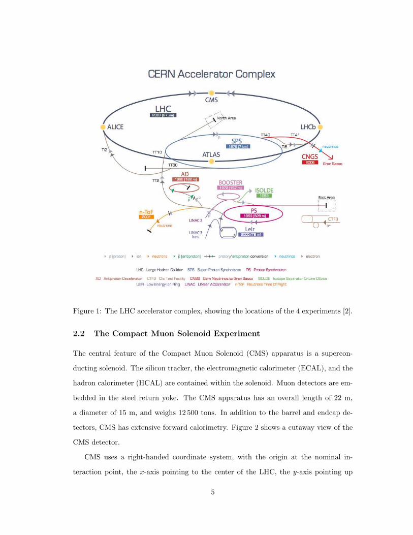
Figure 1: The LHC accelerator complex, showing the locations of the 4 experiments [2].
2.2 The Compact Muon Solenoid Experiment
The central feature of the Compact Muon Solenoid (CMS) apparatus is a supercon-
ducting solenoid. The silicon tracker, the electromagnetic calorimeter (ECAL), and the
hadron calorimeter (HCAL) are contained within the solenoid. Muon detectors are em-
bedded in the steel return yoke. The CMS apparatus has an overall length of 22 m,
a diameter of 15 m, and weighs 12 500 tons. In addition to the barrel and endcap de-
tectors, CMS has extensive forward calorimetry. Figure 2 shows a cutaway view of the
CMS detector.
CMS uses a right-handed coordinate system, with the origin at the nominal in-
teraction point, the x-axis pointing to the center of the LHC, the y-axis pointing up
5

(perpendicular to the LHC plane), and the z-axis along the counterclockwise-beam di-
rection. The polar angle, θ, is measured from the positive z-axis and the azimuthal
angle, φ, is measured in the x-y plane. Pseudorapidity is defined as η = − ln[
tan(
θ2
)]
.
In the following sections the different subdetectors are described. A much more
detailed description of CMS can be found elsewhere [3].
Compact Muon Solenoid
Pixel Detector
Silicon Tracker
Very-forwardCalorimeter
Electromagnetic Calorimeter
HadronicCalorimeter
Preshower
Muon Detectors
Superconducting Solenoid
Figure 2: The CMS Detector [3].
2.2.1 The Solenoid
The superconducting solenoid provides a magnetic field of 3.8 T. This high magnetic
field provides the bending power to accurately measure the momentum of high energy
charged particles. The solenoid has an internal diameter of 6 m, a length of 12.5 m, and
contains the tracking and calorimeter detectors. The solenoid has the capacity to store
2.6 GJ of energy at full current and weighs 220 tons. The flux is returned through an
6
iron return yoke, which consists of 5 wheels and 2 endcaps, composed of 3 disks each,
and weighs 10,000 tons. The muon chambers are integrated within the return yoke.
2.2.2 The Silicon Tracker
The silicon tracker consists of a pixel detector in the center, surrounded by a strip
tracker. The pixel detector consists of 3 barrel layers and 2 endcap disks on each
side, with 65 million channels. The strip tracker is divided into the Tracker Inner Barrel
(TIB), the Tracker Inner Disks (TID), the Tracker Outer Barrel (TOB), and the Tracker
EndCaps (TEC), with a total of 10 million channels. The layout of the tracker is shown
in Figure 3.
The sensors used in the strip tracker are single-sided p-on-n type float zone silicon
microstrip sensors. In the TIB, TID, and the four inner rings of the TECs thin sensors
with a thickness of 320 µm are used. Thicker sensors with a thickness of 500 µm are used
in the TOB and the outer three rings of the TECs. There are “double sided modules”
where two modules are mounted back-to-back with a stereo angle of 100 mrad.
The TIB consists of 4 layers, at radii of 255.0 mm, 339.0 mm, 418.5 mm, and
498.0 mm, respectively from the beam axis. They extend from -700 mm to +700 mm
along the z axis. The two inside layers have double sided modules with an 80 µm strip
pitch, while the two outer layers have single sided modules with a strip pitch of 120 µm.
The TID consists of two sets of three disks, on either end of the TIB. The three disks
range in distance from 800-900 mm in z, and cover a range of radii from 200-500 mm.
The mean strip pitch varies from 100 µm to 141 µm. The two inner rings have double
sided modules, while the outer disk has single sided modules.
The TOB consist of 6 layers, placed at radii of 608, 692, 780, 868, 965, and 1080 mm
from the beam axis. They cover the range from -1090 mm to +1090 mm along the z axis.
The strip pitch of the inner four layers is 183 µm, and 122 µm for the outer two layers.
The inner two layers have double sided modules, while the outer four layers have single
sided modules. Each TEC has nine disks, covering a range of radii from 220-1135 mm
7
and placed between 1240 mm and 2800 mm in z. The modules are arranged in seven
rings around the beam axis. The mean strip pitch varies from 97 µm to 184 µm. The
outer six disks have a slightly larger inner radius than the first three in order to leave
space for the insertion of the pixel detector.
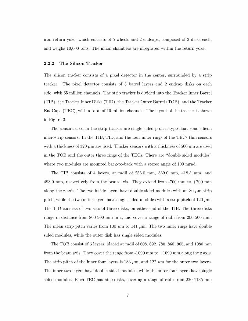
The pixel detector is discussed in much more detail in Chapter 3.
Figure 3: Layout of the tracker, showing the pixel detector, TIB, TID, TOB, andTEC [3].
The main tasks of the silicon detector are tracking and vertexing. The silicon strip
tracker measures charged particles within the |η| < 2.5 pseudorapidity range. The pixel
detector provides 3 space points for each track up to |η| < 2.4. The strip tracker inner
barrel and disks provide up to 4 r − φ measurements, while the outer barrel provides
another 6 r−φ measurements. The strip tracker end caps give up to 9 φ measurements.
This layout ensures at least 9 strip tracker hits for each track, with at least 4 of those
being two dimensional. Figure 4 shows the number of strip tracker hits per track as a
function of |η|.
The tracker provides an impact parameter resolution of ∼ 15 µm and a transverse
momentum (pT) resolution of about 1.5% for 100 GeV/c particles [3].
The vertexing and tracking performance has been studied during the early data
taking period at√s = 7 TeV [4]. The primary vertex resolutions for vertices with more
8

Figure 4: Number of measurement points in the strip tracker as a function of pseudora-pidity . Filled circles show the total number (back-to-back modules count as one) whileopen squares show the number of stereo layers [3].
than 30 tracks are found to be around 25 µm in x and y, and around 20 µm in z.
Figure 5 shows the primary vertex resolutions in x, y, and z as a function of the number
of tracks in the vertex.
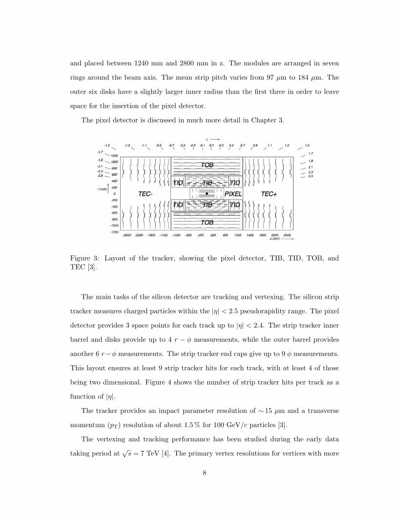
The resolution of the track impact parameter depends on the pT and η of the track.
The impact parameter resolution improves for tracks with higher pT since they are
less affected by multiple scattering. Tracks at higher values of |η| travel through more
material, and so the multiple scattering effects are increased, leading to a degradation
in the impact parameter resolution. The measured impact parameter resolutions as a
function of the track pT are shown in Figure 6, while they are shown as a function of η
in Figure 7. The dip in the longitudinal impact parameter resolution at |η| = 0.5 is due
to the fact that at this angle, the particle deposits its charge in more than one pixel.
The position is then determined by the charge barycenter, improving the resolution.
2.2.3 The Electromagnetic Calorimeter
The electromagnetic calorimeter (ECAL) is made of scintillating lead tungstate (PbW04)
crystals. The signal is read out by avalanche photodiodes in the barrel section (EB)
9

(a) (b)
(c)
Figure 5: Primary vertex resolution in x (a), y (b), and z (c) as a function of the numberof tracks [4].
and vacuum phototriodes in the endcaps (EE). The ECAL provides coverage in pseu-
dorapidity |η| < 1.479 in the EB and 1.479 < |η| < 3.0 in the EE. A preshower detector
consisting of two planes of silicon sensors interleaved with a total of 3X0 of lead is
located in front of the EE, where X0 is the radiation length. The ECAL has an energy
resolution of better than 0.5% for unconverted photons with transverse energies above
100GeV. The layout of the ECAL is shown in Figure 8.
The EB is made up of 61,200 crystals formed into 36 “supermodules”, each con-
taining 1700 crystals, and two endcaps, made up of almost 7,324 crystals each. Each
10

Figure 6: Track transverse (left) and longitudinal (right) impact parameter resolutionas a function of the track pT [4].
crystal is tapered, with an area of 22x22 mm2 at the front face and 26x26 mm2 at the
back face. The crystals are arranged in a semi-projective array, so that the axes make
an angle of approximately 3 with respect to the vector from the center of the detector,
in order to avoid having the cracks aligned with the particle trajectories. The distance
between the centers of the front faces of the crystals and the nominal interaction point
is 1.29 m.
Each endcap contains 7,324 crystals. The crystals are grouped into groups of 5x5
crystals to form supercrystals. The endcaps are divided into two “Dees” each, which
have 3,662 crystals. Each Dee contains 138 supercrystals and 18 partial supercrystals
along the inner and outer edges. The crystal faces are 315.4 cm from the interaction
point, and are pointed toward a spot 1300 mm farther than the interaction point. This
gives angles between 2-8.
The preshower detector is a sampling calorimeter, with two layers covering the range
1.653 < |η| < 2.6. The purposes of the preshower detector are to identify neutral pions
in the endcaps, help identify electrons from minimum ionizing particles, and improve
the position resolution for electrons and photons. It is made of alternating layers of
lead radiators and silicon strip sensors. The lead radiators initiate the shower, while the
11
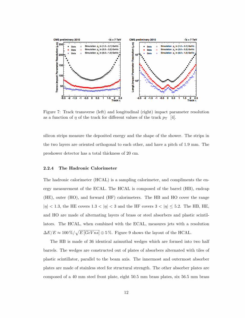
Figure 7: Track transverse (left) and longitudinal (right) impact parameter resolutionas a function of η of the track for different values of the track pT [4].
silicon strips measure the deposited energy and the shape of the shower. The strips in
the two layers are oriented orthogonal to each other, and have a pitch of 1.9 mm. The
preshower detector has a total thickness of 20 cm.
2.2.4 The Hadronic Calorimeter
The hadronic calorimeter (HCAL) is a sampling calorimeter, and compliments the en-
ergy measurement of the ECAL. The HCAL is composed of the barrel (HB), endcap
(HE), outer (HO), and forward (HF) calorimeters. The HB and HO cover the range
|η| < 1.3, the HE covers 1.3 < |η| < 3 and the HF covers 3 < |η| ≤ 5.2. The HB, HE,
and HO are made of alternating layers of brass or steel absorbers and plastic scintil-
lators. The HCAL, when combined with the ECAL, measures jets with a resolution
∆E/E ≈ 100%/√
E [GeV ns]⊕ 5%. Figure 9 shows the layout of the HCAL.
The HB is made of 36 identical azimuthal wedges which are formed into two half
barrels. The wedges are constructed out of plates of absorbers alternated with tiles of
plastic scintillator, parallel to the beam axis. The innermost and outermost absorber
plates are made of stainless steel for structural strength. The other absorber plates are
composed of a 40 mm steel front plate, eight 50.5 mm brass plates, six 56.5 mm brass
12

Figure 8: Layout of the ECAL including the barrel, endcaps, and preshower.
plates, and a 75 mm steel back plate. The light from the scintillators is collected with
wavelength shifting fibers embedded in the scintillators, which are spliced to clear fibers
when they leave the scintillator and are read out by hybrid photodiodes.
The amount of material for the HB is limited by the ECAL and the solenoid, so
the HO is located outside of the solenoid to contain the hadronic shower in the central
psuedorapidity region. The HO is the first sensitive layer in each of the five iron return
yoke rings. In the central ring, there are two layers of scintillator on either side of a
19.5 cm piece of iron. All other rings have a single HO layer.
The HF is located 11.2 m from the interaction point, with the inner radius at 12.5
cm from the beamline. Since the HF is at such high pseudorapidity it is exposed to
large particle fluxes. To account for the harsh environment, quartz fibers were chosen
as the active material. The detector operates by the Cherenkov effect. The calorimeter
is composed of 5 mm steel absorber plates with the fibers inserted into grooves. The
fibers run parallel to the beamline. Half of the fibers run the entire length of the HF,
while the other half begin at 22 cm from the front of the detector. This is to distinguish
13

between electrons and photons, which deposit almost all of their energy in the front of
the detector, from the hadrons, which deposit approximately equal amounts of energy
in the front and back segments.
Figure 9: Longitudinal view of the CMS detector showing the positions of the hadronbarrel (HB), endcap (HE), outer (HO) and forward (HF) calorimeters.
2.2.5 The Muon System
The detection and measurement of muons has always been one of the central goals of
the CMS detector. The muon system covers the pseudorapidity range |η| < 2.4, and is
composed of Drift Tubes (DTs), Cathode Strip Chambers (CSCs), and Resistive Plate
Chambers (RPCs). The muon system has three main purposes: muon identification,
momentum measurement, and triggering. Matching the muons to the tracks measured
in the silicon tracker results in a transverse momentum resolution between 1 and 5%,
for pT values up to 1 TeV/c. The muon detection system has nearly 1 million electronic
channels.
The DTs cover the barrel region, η < 1.2. In this region the magnetic field is uniform
and the rate is low, so standard rectangular drift tube cells are used. They are organized
into 4 stations and are located between the layers of the iron return yoke. The first three
stations each contain 2 groups of 4 chambers that measure the muon position in the
r−φ plane, and another 4 chambers which measure the muon position in the z direction.
14

The fourth station does not have the 4 z-position chambers.
The CSCs are used in the endcap region (0.9 < η < 2.4) because of the high rates
and background, and non-uniform magnetic field. The CSCs are fast, finely segmented,
and radiation resistant. They are multiwire proportional chambers, consisting of 6 lay-
ers of anode wire planes interleaved with 7 cathode strip planes. Each endcap has 4
CSC stations, with the chambers perpendicular to the beamline and located between
the return yoke plates. The cathode strips run radially outward, and provide the mea-
surement in the r − φ plane. The anode wires run approximately perpendicular to the
cathode strips and are also read out to give a measurement in η.
The DTs and CSCs can both easily trigger on the pT of the muon, but due to the
large uncertainty in the background rates and the ability to measure the correct beam-
crossing time a complementary trigger system was designed using RPCs. The RPCs are
parallel plate gas chambers, operated in avalanche mode. They have a very good time
resolution, but a coarser position resolution than the DTs or CSCs. There are 6 layers
of RPCs in the barrel region: 2 in each of the first 2 muon stations and 1 in each of the
last 2 muon stations. In the endcap region there are 3 layers of RPCs, covering up to
η < 1.5.
2.2.6 The Forward Detectors
The very forward angles are covered by the Centauro And Strange Object Research
(CASTOR) detector and the Zero Degree Calorimeter (ZDC). CASTOR covers the
range from (5.3 < |η| < 6.6), while the ZDC covers (|η| > 8.3). Two extra tracking sta-
tions, built by the TOTal Elastic and diffractive cross section Measurement (TOTEM)
experiment, are placed at forward rapidities (3.1 < |η| < 4.7 and 5.5 < |η| < 6.6).
The ZDC and CASTOR calorimeters are Cherenkov sampling calorimeters, each
consisting of electromagnetic (EM) and hadronic (HAD) sections. The calorimeters
are built from tungsten absorber plates, alternated with fused silica quartz plates in
CASTOR and quartz fibers in the ZDC, and read out by photomultiplier tubes. The
15
plates are placed at a 45 angle with respect to the incoming particles’ direction to
maximize the light signal. The CASTOR geometry is shown in Figure 10. CASTOR is
placed 14.38 m from the interaction point. The ZDC is located approximately 140 m
from the interaction point. Figure 11 shows the geometry of the ZDC.
Figure 10: Side cutaway view of CASTOR showing the EM and HAD sections.
2.2.7 The Trigger System
During proton-proton collisions, the LHC is designed to have a beam crossing interval
of 25 ns, which corresponds to a crossing rate of 40 MHz. At the design luminosity of
1034cm−2s−1, there are approximately 20 collisions per bunch crossing. The amount of
data associated with this large number of events is impossible to store, and the rate must
be reduced. In CMS this is accomplished with a two level trigger system, the Level-1
(L1) trigger and the High-Level Trigger (HLT). The combined L1 and HLT system is
designed to be able to reduce the rate by a factor of at least 106.
The L1 trigger is mainly hardware based and has a design output rate limit of 100
16
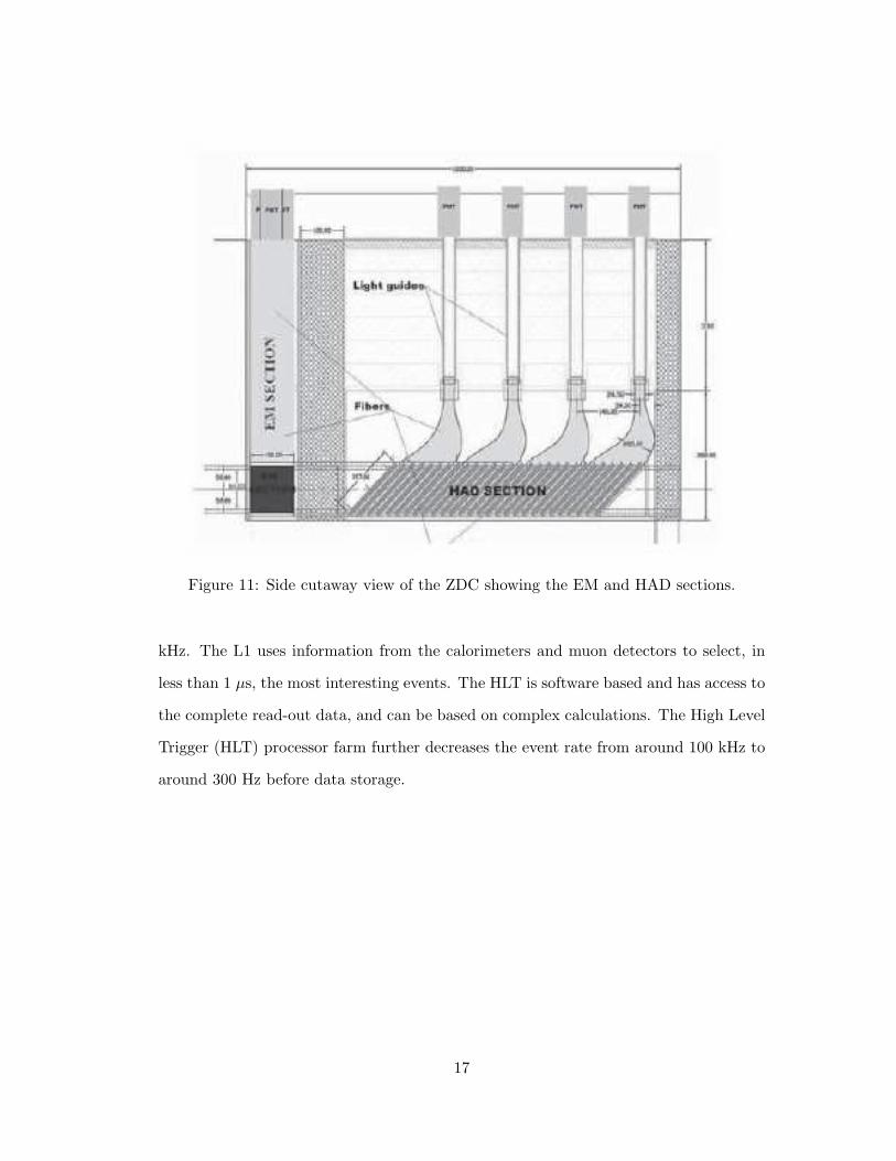
Figure 11: Side cutaway view of the ZDC showing the EM and HAD sections.
kHz. The L1 uses information from the calorimeters and muon detectors to select, in
less than 1 µs, the most interesting events. The HLT is software based and has access to
the complete read-out data, and can be based on complex calculations. The High Level
Trigger (HLT) processor farm further decreases the event rate from around 100 kHz to
around 300 Hz before data storage.
17
3 The CMS Pixel Detector
The silicon pixel detector is the closest subdetector to the interaction point. The main
goal of the pixel detector is to provide very good impact parameter resolution and
vertexing, as well as three spatial points for track reconstruction. The pixels have a size
of 150x100 µm2, with the 100 µm dimension in the r − φ direction in the barrel and
the r direction in the forward disks. The dimensions were chosen to be nearly square
in order to provide similar resolution in both the r − φ and z directions.
The CMS pixel detector is a “hybrid” pixel detector. A hybrid pixel detector consists
of a separate sensor and readout electronics chip, which are designed and manufactured
separately and then bump bonded together. The detector layout, sensors, and readout
electronics are described briefly in the following sections. More details about the design
and construction of the pixel detector can be found elsewhere [38, 3].
3.1 Detector Layout
The pixel detector consists of a barrel section (BPix) with 3 cylindrical layers at radii
of 4.4 cm, 7.3 cm, and 10.2 cm, and two forward disks on each end (FPix), at a distance
of 34.5 cm and 46.5 cm from the center of the CMS detector. The inner radius of the
forward disks is at 6 cm, and the outer radius is at 15 cm. The pixel detector covers the
pseudorapidities −2.5 < η < 2.5, and provides three space tracking points. The layout
is shown in Figure 12.
The BPix has a total of 48 million channels and covers an area of 0.78 m2. There are
about 800 modules in the barrel section. There are 672 full modules, and the remaining
modules are half modules, located where the two halves of the barrel join. A full module
consists of a silicon sensor bump bonded to 16 readout chips (ROCs), while a half module
has only 8 ROCs. Each ROC consists of 52x80 pixels of size 150x100 µm2 [38, 3].
The FPix has a total of 18 million channels and covers an area of 0.28 m2. The
forward disks are divided into plaquettes, which consist of a single sensor bump bonded
18
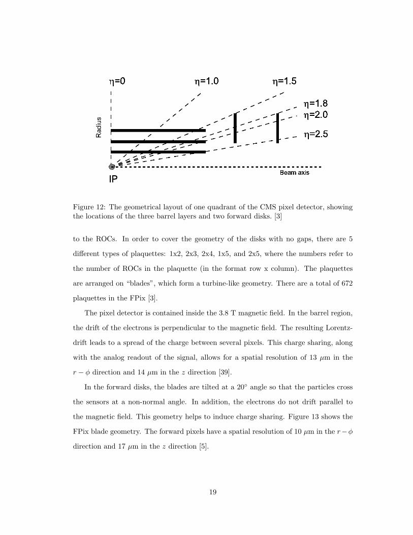
Figure 12: The geometrical layout of one quadrant of the CMS pixel detector, showingthe locations of the three barrel layers and two forward disks. [3]
to the ROCs. In order to cover the geometry of the disks with no gaps, there are 5
different types of plaquettes: 1x2, 2x3, 2x4, 1x5, and 2x5, where the numbers refer to
the number of ROCs in the plaquette (in the format row x column). The plaquettes
are arranged on “blades”, which form a turbine-like geometry. There are a total of 672
plaquettes in the FPix [3].
The pixel detector is contained inside the 3.8 T magnetic field. In the barrel region,
the drift of the electrons is perpendicular to the magnetic field. The resulting Lorentz-
drift leads to a spread of the charge between several pixels. This charge sharing, along
with the analog readout of the signal, allows for a spatial resolution of 13 µm in the
r − φ direction and 14 µm in the z direction [39].
In the forward disks, the blades are tilted at a 20 angle so that the particles cross
the sensors at a non-normal angle. In addition, the electrons do not drift parallel to
the magnetic field. This geometry helps to induce charge sharing. Figure 13 shows the
FPix blade geometry. The forward pixels have a spatial resolution of 10 µm in the r−φ
direction and 17 µm in the z direction [5].
19
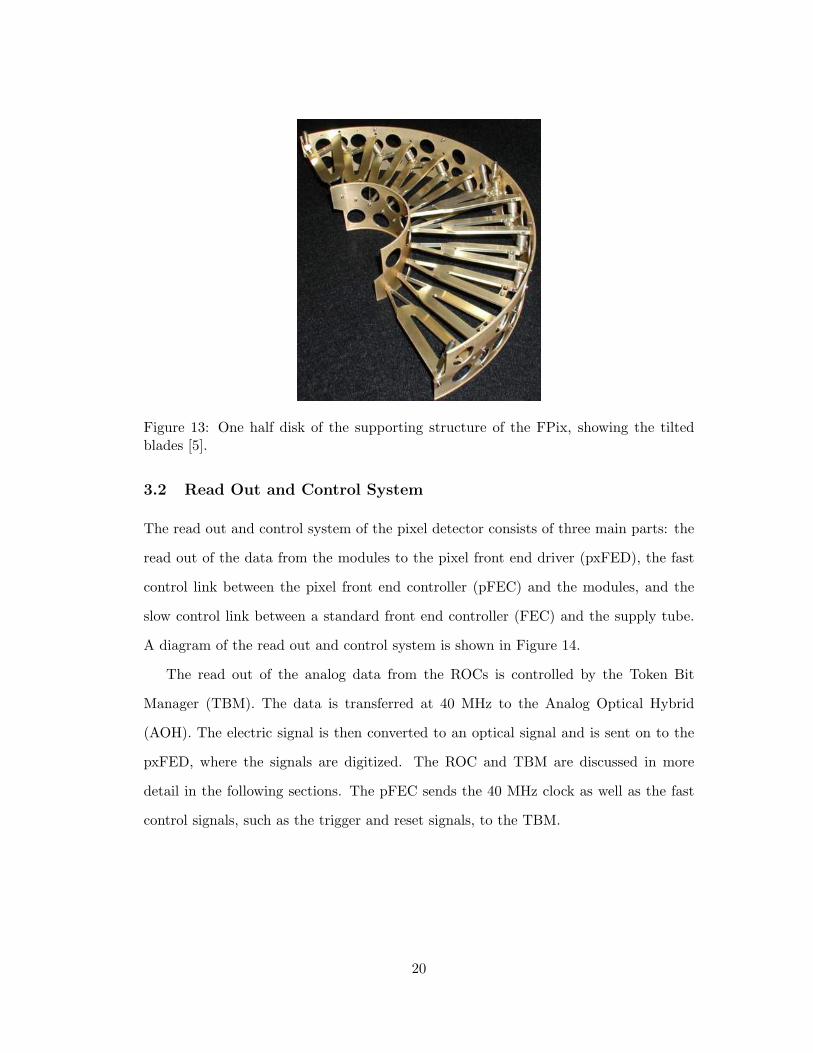
Figure 13: One half disk of the supporting structure of the FPix, showing the tiltedblades [5].
3.2 Read Out and Control System
The read out and control system of the pixel detector consists of three main parts: the
read out of the data from the modules to the pixel front end driver (pxFED), the fast
control link between the pixel front end controller (pFEC) and the modules, and the
slow control link between a standard front end controller (FEC) and the supply tube.
A diagram of the read out and control system is shown in Figure 14.
The read out of the analog data from the ROCs is controlled by the Token Bit
Manager (TBM). The data is transferred at 40 MHz to the Analog Optical Hybrid
(AOH). The electric signal is then converted to an optical signal and is sent on to the
pxFED, where the signals are digitized. The ROC and TBM are discussed in more
detail in the following sections. The pFEC sends the 40 MHz clock as well as the fast
control signals, such as the trigger and reset signals, to the TBM.
20

Figure 14: Diagram of the pixel detector read out chain and control system. Moredetails can be found in [3].
3.3 Modules
Figure 15 shows photographs of a barrel pixel full module and a half module, as well as
a diagram showing all the main components of a module. The module is composed of
the sensor, the ROCs, a high density interconnect (HDI) containing the TBM, a power
cable, a Kapton signal cable, and silicon nitride base strips to attach the module to the
mechanical structure. The main components are described in the following sections.
3.3.1 The Token Bit Manager
The TBM controls a group of ROCs. In the barrel, the TBM is located on the module
and controls either 8 or 16 ROCS, depending on the location and layer. In the forward
21

Figure 15: Picture of a BPix half module (left) and full module (right). The centershows an exploded view of a module, with the different components labeled.
disks, the TBM is located on the blade and controls either 21 or 24 ROCS, depending
on which side of the blade it is on.
The TBM is responsible for sending the clock to the ROCs and initiating the read
out of the module. When the TBM receives a Level 1 trigger, it passes the trigger to
the ROCs, to tell the ROC not to delete the data for the triggered event. After some
time the TBM passes a token to each ROC in series. When the ROC receives the token,
it reports any hits and then passes the token to the next ROC.
The read out of a full module, shown in Figure 16, consists of a TBM header, a
header for each ROC, followed by any hits from that ROC, and a TBM trailer. The
TBM header begins with a very low signal, called “ultra-black”, for 3 clock cycles,
followed by a 1, called “black”, to signify the beginning of the readout. Following this
are four clock cycles containing the 8-bit encoded analog event number [40]. After the
TBM header, each ROC adds a header followed by any hits.
22

Figure 16: A read out of a full module with a hit in ROC 0, showing the TBM header,hit information from ROC 0, headers from the remaining ROCs, and TBM trailer.
3.3.2 The Readout Chip
The readout chip is a custom designed application-specific integrated circuit (ASIC). It
contains 52x80 pixels and is commercially fabricated in a 0.25 µm complementary metal
oxide semiconductor (CMOS) process [3]. The ROC has several purposes. It provides
zero suppression with an individually adjustable threshold in each pixel unit cell. The
ROC also amplifies and buffers the signal from the sensor. It also provides the Level 1
trigger information and discards any hits which do not have a corresponding L1 trigger.
The ROC has three main blocks: the array of pixel unit cells (PUCs), the double
column periphery, and the chip periphery. Figure 17 is a picture of the ROC showing
these three blocks as well as a double column. The chip periphery contains various
control and supply circuits. The double column periphery controls the read out of the
double columns, including transfering the hit information from the pixel to the storage
23

buffers and the trigger verification [41].
Figure 17: The read out chip.
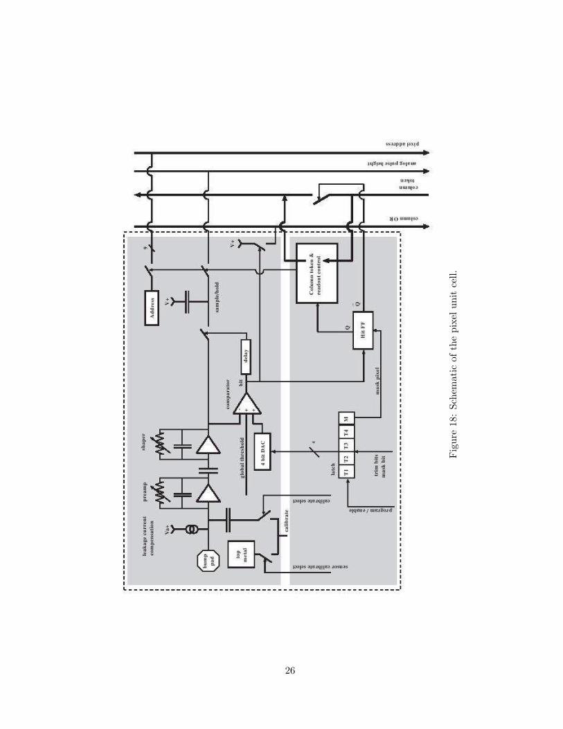
The schematic of a pixel unit cell is shown in Figure 18. The PUC consists of an
analog part (top) and a digital logic part (bottom). The signal enters the PUC from
the sensor through the bump bond. A calibrate signal can also be injected, either by a
4.8 fF capacitor connected directly to the amplifier, or via the sensor through the air
gap between a top metal pad on the ROC and the sensor. The direct signal injection
can be used to adjust the pixel threshold, while the indirect injection can be used to
test the bump bonds.
The signal passes through a two-stage preamplifier and shaper system. The signal
then passes through a comparator, which provides the zero suppression. There is a 4-bit
24

digital to analog converter (DAC) to adjust the pixel’s individual threshold, as well as
a mask bit to disable noisy pixels. Once the signal passes the comparator it is stored
in a sample-and-hold circuit. The double column periphery is notified, and the pixel
waits for the column readout token. A double column can accept up to three hits before
the column readout, and is insensitive to any further hits. When the PUC receives the
column readout token, it sends the analog signal and the pixel row address to the double
column periphery and passes the token.
The ROC handles the complete pixel address encoding for each hit, and sends this
address along with the analog signal pulse height to the TBM. The digital pixel address
is encoded in 6 level analog values, which are shown in Figure 19.
An example of a read out of a ROC with one hit is shown in Figure 20. The ROC
header is three clock cycles and contains an ultra-black, a black, and a signal inversely
proportional to the last addressed DAC value [41]. The pixel address is encoded in the
5 clock cycles following the ROC header. The first two clock cycles are the encoded
double column, and the next three contain the encoded row. Finally, the analog pulse
height is in the last clock cycle. In the case of multiple hits, the address of the next hit
pixel would immediately follow the pulse height of the previous hit.
25
Figure
18:Schem
atic
ofthepixel
unit
cell.
26
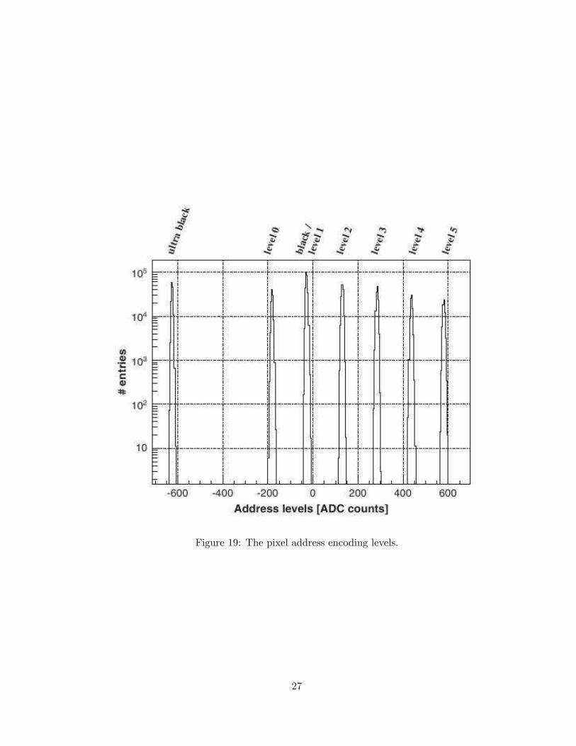
Figure 19: The pixel address encoding levels.
27

Figure 20: A read out of a hit from a ROC.
28

3.3.3 The Sensor
The basic operating principle of silicon sensors is discussed in Chapter 4. The sensor is
made from 285 µm thick diffused oxygen float zone (DOFZ) silicon, as oxygen-enriched
silicon has been shown to have better radiation hardness [1]. The BPix sensors were
produced by CiS, using silicon with the 〈111〉 orientation and a resistivity of 3.7 kΩcm [7].
The sensor has a depletion voltage of 50-60 V. The FPix sensors were produced by
Sintef, and consist of silicon with the 〈100〉 orientation and a resistivity of approximately
5 kΩcm. The depletion voltage is around 50 V [42].
The n+-in-n sensors consist of highly doped n-implants in an n-type substrate, and
the pn-junction on the backside along with a multiple guard ring structure. This design
requires double-sided processing, which increases the cost, but allows the edges of the
sensor to be at ground potential so that the detector can be operated at high bias
voltages (up to 600 V).
When a charged particle crosses the sensor material, it ionizes the silicon and pro-
duces electron-hole pairs. The electrons and holes drift in opposite directions, due to
the internal electric field. This is shown in Figure 21. A minimum ionizing particle
(mip) crossing perpendicularly through the sensor deposits a charge of approximately
22,000 electrons. The n-type pixels were chosen in order to collect electrons, which
have a higher mobility. This reduces the effects of charge trapping, and thereby ensures
a substantial signal even after high hadron fluences. After irradiation, the depletion
region will start from the n+ implants, and will allow operation of the detector with
moderate bias voltages.
The entire pixel detector is located within the magnetic field of the CMS solenoid
magnet, and the charge carriers are deflected by the Lorentz force. The deflection
angle of the charge carriers is called the Lorentz angle. It depends on the mobility of
the charge carriers, which in turn depends on the electric field inside the sensor. The
Lorentz angle was measured in a test beam [7], and the measured angle as a function
of the bias voltage is shown in Figure 22.
29

In the FPIX open ring p-stops were used for the interpixel isolation. The opening
in the p-stop ring provides a high resistance path between pixels after full depletion.
The p-stop ring has a width of 8 µm, and the gap between the implants is 12 µm. A
picture of four FPix pixels is shown in Figure 23. The seven different sensor designs
needed for a blade, to accomodate the different number and arrangements of ROCs, are
all produced on one wafer.
In the BPix, a moderated p-spray isolation is used. This technique combines a uni-
form p-spray implantation with a traditional p-stop, but does not require any additional
mask. The technique is described in more detail in [43]. The gap between the implants
is 20 µm. The BPix also include a “bias dot”, which provides a high resistance punch-
through bias structure. This allows IV measurements on the wafer to assess the sensor
quality during production. A picture of four BPix pixels with the visible structures
labeled is shown in Figure 24.
3.4 Mechanics and Cooling
The pixel barrel system is composed of the modules, their support structure, and the
supply tubes to carry services from outside of the tracker volume to the detector. A
drawing of one of the supply tubes is shown in Figure 25. The barrel has a length of
570 mm and is centered around the interaction region. The length of the total system,
including the supply tubes, is 5.60 m. The barrel is divided vertically into two half
cylinders, in order to be installed around the beam pipe and its supports. The two half
cylinders are electrically separate and operate almost independently. Each half cylinder
can slide into place in CMS on rails around the beam pipe. A schematic of one half
barrel is shown in Figure 26.
The main structure is provided by the aluminum cooling tubes. The cooling tubes
have a wall thickness of 0.3 mm. The tubes have a trapezoidal cross section. The
aluminum cooling tubes are welded to an aluminum container which distributes the
cooling fluid through the detector.
30

The cooling fluid used in the current detector is C6F14. It is foreseen to cool the
detector down to a temperature of -10 C. So far, the detector has been operated at a
temperature of 17 C in 2010 and 2011, and at 7 C in 2012.
Carbon fiber blades with a thickness of 0.24 mm are glued to the top and bottom
of two adjacent tubes. The individual segments are connected on each end to flanges
to provide the half barrel structure. The end flanges are fiberglass frames filled with
foam and covered with carbon fiber blades. The end flanges contain connectors for the
module cables and for supplying power to the modules.
3.5 Material Budget
Any material in the path of the particles traversing the detector can contribute to mul-
tiple scattering, bremsstrahlung, photon conversions, and nuclear interactions. These
effects can reduce the accuracy of the reconstruction of the tracks of the incoming par-
ticles. Therefore it is necessary to keep the amount of material in the tracker as low as
possible.
The amount of material in the path of the particles is called the material budget. It
is usually measured in terms of the fraction of radiation lengths, x/X0. The radiation
length, X0, is defined as the mean distance in which an electron loses all but 1/e of its
energy by bremsstrahlung.
The material budget for the tracker as a whole, as well as the pixel barrel detector,
is shown in Figure 27. The material budget is broken into the different categories of
the material. The main contribution of the pixel barrel to the overall tracker material
budget is at |η| > 1.2. This comes from the end flange and the inner part of the supply
tube [8].
31
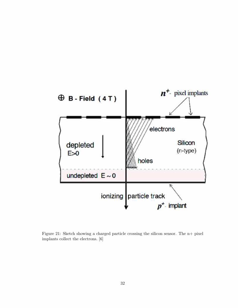
Figure 21: Sketch showing a charged particle crossing the silicon sensor. The n+ pixelimplants collect the electrons. [6]
32
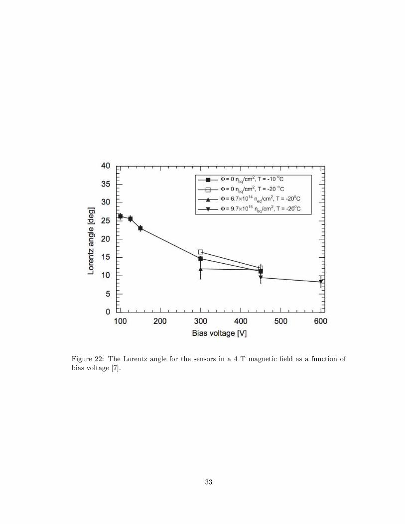
Figure 22: The Lorentz angle for the sensors in a 4 T magnetic field as a function ofbias voltage [7].
33

Figure 23: Picture of four pixels in the same double column for the FPix. The pixelshave a pitch of 100 x 150 µm. [3]
34

Figure 24: Picture of four pixels in the BPix. The pixels have a pitch of 100 x 150 µm.The indium bumps have been deposited but not reflown, and are visible. [3]
35

Figure 25: Drawing of one of the supply tubes. [3]
Figure 26: A sketch of one half cylinder of the barrel pixels. [3]
36

Figure 27: Left: Material budget for the whole CMS tracker, showing the varioussubdetector contributions. Right: Material budget for the pixel barrel detector, showingthe various categories of material. [8]
37

4 Radiation Damage in Silicon Detectors
One of the challenges of tracking at colliders such as the LHC is designing detectors
which can withstand the high radiation environment. Silicon detectors have the capabil-
ity to be highly segmented, which makes them good choices for the innermost trackers,
since a high granularity is important for vertexing and tracking in a dense environment
such as the LHC. As commercial vendors are widely available and there is a lot of indus-
trial experience in manufacturing silicon based devices, they are relatively inexpensive
to produce. In addition, they have been shown to be sufficiently resistant to radiation
damage for all previous applications, but they do degrade during the operation of the
LHC. In order to fulfill the LHC specific requirements for long-term operation, it is
important to study the degradation of the performance of silicon-based detectors due
to the effects of radiation damage and to establish their operational limits [1].
4.1 Basic Properties and Operating Principle of Silicon Sensors
Before discussing the effects of radiation on the silicon sensors, it is necessary to discuss
the basic properties of silicon sensors. Silicon atoms have four valence electrons which
contribute to the bonding between atoms. It is possible to replace some atoms in the
crystal lattice with another element which has either three or five valence electrons.
This process is called doping.
In the case of a dopant atom with five valence electrons, four of the electrons are
involved in the bonding, while the fifth electron can be excited by its thermal energy into
a state shared between many atoms, and can move about the lattice. These atoms are
called “donors”. In silicon doped with donor atoms, there is an excess of free electrons.
This is called n-type silicon. In the case of a dopant atom with only three valence
electrons, one of the four bonding sites is left empty. The dopant atoms are called
“acceptors”. This type of material can be described as having an excess of holes which
are free to move about the lattice. This type of silicon is called p-type.
38
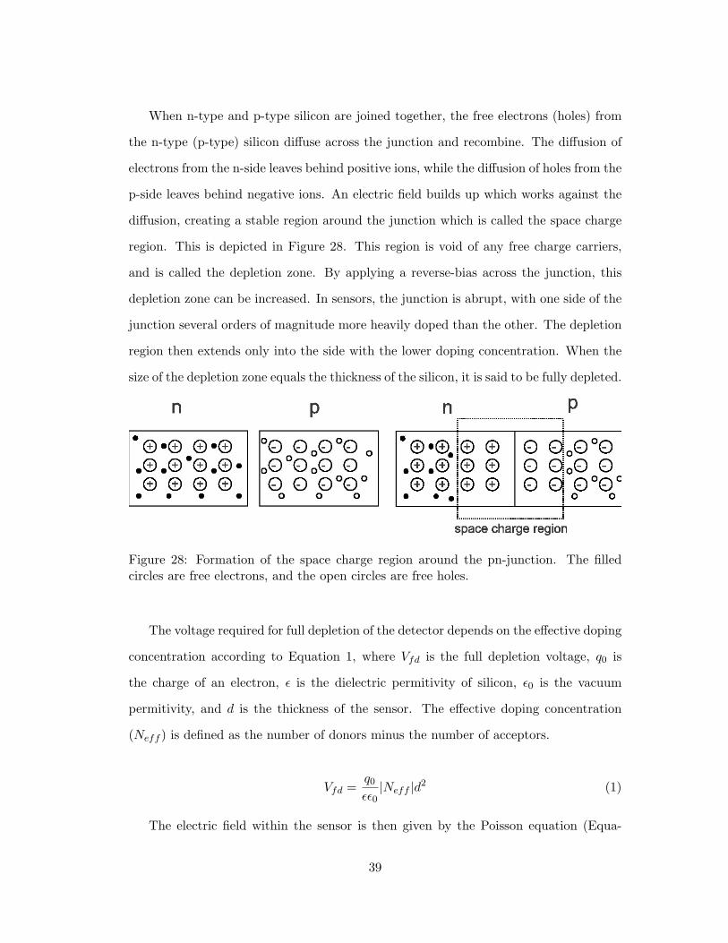
When n-type and p-type silicon are joined together, the free electrons (holes) from
the n-type (p-type) silicon diffuse across the junction and recombine. The diffusion of
electrons from the n-side leaves behind positive ions, while the diffusion of holes from the
p-side leaves behind negative ions. An electric field builds up which works against the
diffusion, creating a stable region around the junction which is called the space charge
region. This is depicted in Figure 28. This region is void of any free charge carriers,
and is called the depletion zone. By applying a reverse-bias across the junction, this
depletion zone can be increased. In sensors, the junction is abrupt, with one side of the
junction several orders of magnitude more heavily doped than the other. The depletion
region then extends only into the side with the lower doping concentration. When the
size of the depletion zone equals the thickness of the silicon, it is said to be fully depleted.
Figure 28: Formation of the space charge region around the pn-junction. The filledcircles are free electrons, and the open circles are free holes.
The voltage required for full depletion of the detector depends on the effective doping
concentration according to Equation 1, where Vfd is the full depletion voltage, q0 is
the charge of an electron, ε is the dielectric permitivity of silicon, ε0 is the vacuum
permitivity, and d is the thickness of the sensor. The effective doping concentration
(Neff ) is defined as the number of donors minus the number of acceptors.
Vfd =q0εε0
|Neff |d2 (1)
The electric field within the sensor is then given by the Poisson equation (Equa-
39

tion 2). It is linear and proportional to Neff .
∇E =−eNeff
εε0(2)
When a charged particle crosses through a depleted sensor, it creates many electron-
hole pairs along its path. These electrons and holes are separated by the electric field
and move towards the n- and p-contacts, respectively. The moving charges induce a
signal on the contact, which is then read out by the readout electronics.
Silicon sensors always have leakage current, caused by the creation of electron-hole
pairs by thermal excitation. Any defects in the silicon lattice act a centers for electron-
hole pairs. The leakage current has an exponential temperature dependence, as shown
in Equation 3. In this equation, Eg is the effective energy gap (1.12 eV), and kb is the
Boltzmann constant [44].
I ∝ T 2e
(
−Eg2kbT
)
(3)
4.2 Damage Mechanisms
The effects of radiation on silicon detectors can be separated into two categories: surface
damage and bulk damage. Surface damage is the result of ionization in the covering lay-
ers of the sensor, and the effects on the overall operation of the CMS pixel detector are
counteracted by the design of the sensors. Bulk damage is the result of non-ionizing en-
ergy loss, i.e. the displacement of nuclei in the silicon lattice, and leads to the observable
degradation in the detector operation and performance.
4.2.1 Surface Damage
Surface damage refers to the defects created in the silicon oxide layer and the interface
between the oxide and the bulk silicon. Surface damage comes mainly from ionization
and the creation of electron-hole pairs in the oxide. As the interface between the oxide
40

and the bulk silicon is already irregular, displacement of single atoms does not signifi-
cantly change the properties of the detector. The main effects of the surface damage are
a build up of positive charge along the interface and an increase in the so-called surface
current. The holes created near the surface are trapped due to their low mobility, while
the electrons are collected. This build up of positive charge is called the “fixed oxide
charge.” This accumulation layer is a few nanometers thick, and change the electric field
distribution in the first few micrometers below the surface. MIPs deposit their energy
evenly throughout the bulk of the sensor, and so surface damage has little impact on
the operation of the detectors for tracking charged particles. The main impact of the
built up surface charge is a change in the electric field close to the surface, which can
cause early breakdown. By creating a layout with small gaps between the pixels, this
effect can be reduced.
4.2.2 Bulk Damage
Bulk damage is caused by particles which interact with the nucleus of an atom in the
silicon lattice. The defects can be described as point and cluster defects, which affect
the silicon in different ways. An incoming particle can knock an atom out of its position
in the lattice. To knock a silicon atom out of its lattice position requires a recoil energy
around 25 eV. For electrons this corresponds to an energy of 260 keV, or an energy of
only 190 eV for protons or neutrons. The space left behind is called a vacancy, while
the atom, which stops between the regular lattice positions, is called an interstitial. The
pair of a vacancy and an interstitial is called a “Frenkel pair” and is a point defect.
This atom can also be called a primary knock on atom (PKA). If the PKA has
enough energy, it can in turn knock out other atoms. At the end of the flight path it
loses a lot of energy in a small volume and creates many defects. Such regions of high
defect density are called cluster defects. A simulation of the path of a PKA through
the silicon lattice is shown in Figure 29, with the point defects shown in red and the
cluster defects shown in blue.
41
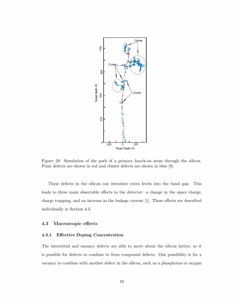
Figure 29: Simulation of the path of a primary knock-on atom through the silicon.Point defects are shown in red and cluster defects are shown in blue [9].
These defects in the silicon can introduce extra levels into the band gap. This
leads to three main observable effects in the detector: a change in the space charge,
charge trapping, and an increase in the leakage current [1]. These effects are described
individually in Section 4.3.
4.3 Macroscopic effects
4.3.1 Effective Doping Concentration
The interstitial and vacancy defects are able to move about the silicon lattice, so it
is possible for defects to combine to form compound defects. One possibility is for a
vacancy to combine with another defect in the silicon, such as a phosphorus or oxygen
42
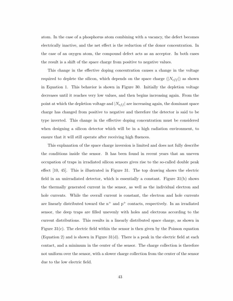
atom. In the case of a phosphorus atom combining with a vacancy, the defect becomes
electrically inactive, and the net effect is the reduction of the donor concentration. In
the case of an oxygen atom, the compound defect acts as an acceptor. In both cases
the result is a shift of the space charge from positive to negative values.
This change in the effective doping concentration causes a change in the voltage
required to deplete the silicon, which depends on the space charge (|Neff |) as shown
in Equation 1. This behavior is shown in Figure 30. Initially the depletion voltage
decreases until it reaches very low values, and then begins increasing again. From the
point at which the depletion voltage and |Neff | are increasing again, the dominant space
charge has changed from positive to negative and therefore the detector is said to be
type inverted. This change in the effective doping concentration must be considered
when designing a silicon detector which will be in a high radiation environment, to
ensure that it will still operate after receiving high fluences.
This explanation of the space charge inversion is limited and does not fully describe
the conditions inside the sensor. It has been found in recent years that an uneven
occupation of traps in irradiated silicon sensors gives rise to the so-called double peak
effect [10, 45]. This is illustrated in Figure 31. The top drawing shows the electric
field in an unirradiated detector, which is essentially a constant. Figure 31(b) shows
the thermally generated current in the sensor, as well as the individual electron and
hole currents. While the overall current is constant, the electron and hole currents
are linearly distributed toward the n+ and p+ contacts, respectively. In an irradiated
sensor, the deep traps are filled unevenly with holes and electrons according to the
current distributions. This results in a linearly distributed space charge, as shown in
Figure 31(c). The electric field within the sensor is then given by the Poisson equation
(Equation 2) and is shown in Figure 31(d). There is a peak in the electric field at each
contact, and a minimum in the center of the sensor. The charge collection is therefore
not uniform over the sensor, with a slower charge collection from the center of the sensor
due to the low electric field.
43
Figure 30: Change in the effective doping concentration as well as the voltage requiredfor full depletion as a function of the fluence [1].
4.3.2 Charge Trapping
The energy levels in the band gap act as traps for charges. Often a charge moving
through the lattice will occupy one of these energy levels for a short time. However, this
time may be longer than the integration time, and so the collected charge is less than
the total deposited charge. This charge-trapping leads to a decreased charge collection
efficiency, and for smaller signals, a decreased detection efficiency [1]. It is essential
to study these changes to determine at what point the sensors are no longer efficient
enough to be used by the experiments.
The different defects induced in the silicon by radiation have been studied on a mi-
croscopic level by several groups [1, 9]. However, these methods are only able to see
shallow traps and so the amount of signal lost by charge trapping can not be predicted
44
well. The charge losses must be measured with macroscopic techniques, such as charge
collection efficiency (CCE) and Transient Current Technique (TCT) measurements. In
this work, the charge losses due to trapping are studied by measuring the charge col-
lection efficiency of sensors which have been irradiated to various fluences. Charge
collection efficiency measurements on irradiated CMS barrel pixel sensors are discussed
in detail in Chapter 5.
4.3.3 Leakage Current
The energy levels created by the defects in the band gap can act as centers for electron-
hole pair generation. This effectively increases the leakage current of the sensor. The
amount of current created (∆I) is proportional to the fluence, according to Equation 4,
where Φeq is the fluence normalized to the damage caused by 1 MeV neutrons (see
Section 4.4) and α is a proportionality constant. The changes in the leakage current are
independent of the initial resistivity and impurity concentration [44].
∆I = αΦeqV (4)
The exponential temperature dependence of the leakage current (Equation 3) still
holds in irradiated sensors. In order to keep the current below acceptable limits and to
avoid thermal runaway, it is necessary to operate irradiated detectors at low tempera-
ture.
4.4 NIEL Scaling
The Non Ionizing Energy Loss (NIEL) hypothesis attempts to allow scaling of the
radiation damage produced by different types of particles and particle energies. The
NIEL hypothesis is based on the assumption that any changes in the material due to
displacement are linearly related to the amount of energy deposited in the collision,
independently of how the defects are distributed or of any annealing which occurs after
45
the initial collision [1]. The non-ionizing energy loss is the amount of energy deposited
in the crystal, excluding the energy that went into ionization, which is reversible. 1 MeV
neutrons are used as the reference particles, and the fluence of any particle is scaled to
the 1 MeV neutron equivalent. Therefore it is common practice to quote fluences in
units of neutron equivalent fluence, neq/cm2.
The scaling can be done by defining a hardness factor κ in order to compare the
amount of damage done by a specific irradiation to the damage which would have oc-
curred from 1 MeV neutrons with the same fluence. The determination of the hardness
factor relies on the fact that the changes in leakage curret are independent of the resis-
tivity and impurity concentration. The 1 MeV neutron equivalent fluence can then be
calculated according to Equation 5.
Φeq = κΦ = κ
∫
φ(E)dE (5)
Here, φ(E) is the energy spectrum of the radiation. The hardness factor is unique to
each radiation source. The hardness factors for the sources used in the measurements
presented in Chapter 5 are listed in Appendix A.
This approach is limited, as neutrons and charged hadrons produce different types
of defects. The main mechanism by which charged hadrons interact with silicon at
low energies is the Coulomb interaction, and they tend to produce mostly point defects.
Neutrons can only interact by elastic scattering with the nucleus and by nuclear reactions
above 1.8 MeV, and they produce more cluster defects [1].
4.5 Annealing
Defects in the silicon lattice are free to move about the lattice due to thermal energy.
The defects can collect at specific locations, such as the surface, or encounter other
defects and combine to form complex defects. Complex defects can also break apart if
they have enough energy to overcome the binding energy holding them together. These
46
processes are called annealing.
During the annealing, the space charge changes. The most successful parametrisa-
tion is the so-called Hamburg model [1]. It describes the change of the space charge by
three components: short term annealing, stable damage, and long term annealing. It
can be described as a function of the fluence and time by Equation 6.
∆Neff (Φeq, t(Ta)) = NA(Φeq, t(Ta)) +NC(Φeq, t(Ta)) +NY (Φeq, t(Ta)) (6)
Here NA is the short term component, NC is the stable damage component, and NY is
the long term component. An example of the change in the effective doping concentra-
tion as a function of the annealing time is shown in Figure 32.
The short term annealing is also often called “beneficial annealing” because it is
associated with a decrease in the absolute value of the space charge. This takes place
over a period of a few days. In long term annealing, the space charge becomes more
negative, and is often called “reverse annealing.” The long term annealing can be frozen
by keeping the detector at low temperatures. Therefore the most important component
for the LHC experiments is the stable damage. The stable damage is not influenced by
the operating temperature of the detector, but it has been shown that it is different for
different types of silicon. In particular, the addition of oxygen to the silicon reduced
the stable damage [1].
The annealing rates are highly dependent on temperature. Therefore, in order to be
sure that samples are at the same state, the annealing history must be understood. In
general, all samples used in this work were subjected to an identical annealing process,
and stored at low temperature to halt any further annealing.
4.6 Estimated Requirements for CMS Pixel Detector Sensors
The radiation environment at the LHC is extremely harsh, so there were dedicated
studies during the design phase of the detector to determine the amount of radiation
47

which the different subdetectors needed to be able to withstand. The pixel detector is
the closest subdetector to the collision point, and so subjected to the highest amount of
radiation. Eventually the pixel detector will need to be replaced, and so was designed
so that it can be removed and replaced relatively easily during a shutdown period.
There are several factors which limit the lifetime of the sensors. The increase in
charge trapping eventually means that the signal is too low to pass the threshold. In-
creasing the bias voltage can help recover the signal, but leads to a decrease in the
charge sharing between pixels. For high voltages the spatial resolution degrades until it
becomes the binary resolution; that is, the resolution given purely by the pixel dimen-
sions, without any charge sharing, which is given by the pitch/√12. In addition, the
available bias voltage is currently limited by the connectors and power supplies which
carry the voltage to the detector to a maximum of 600 V.
At the full LHC design luminosity, it was estimated that the pixel detector would be
subjected to a fluence of 3 x 10¹⁴ neq/cm2 per year in the first layer, and 1.2 x 10¹⁴ and
0.6 x 10¹⁴ neq/cm2 per year in the second and third layers, respectively [7]. The current
pixel detector was designed to withstand a fluence of 6 x 10¹⁴ neq/cm2 , corresponding
to approximately 250 fb−1 of integrated luminosity for the innermost layer. As of the
writing of this dissertation, the most recent schedules plan for the pixel detector to be
replaced during the extended year-end technical stop in 2016-2017, after an integrated
luminosity of approximately 100 fb−1.
48

Figure 31: Illustration of the double peak effect. The p+-contact is at x = 0, and then+-contact is at x = d. (a) Electric field in an unirradiated detector. (b) Thermallygenerated current, with the electron (red) and hole (green) currents. (c) Space chargedistribution in an irradiated detector. (d) Electric field in an irradiated detector. Figurereproduced from [10].
49

Figure 32: Change in effective doping concentration as a function of annealing time,taken from [1].
50
5 Sensor Measurements
In order to make measurements of the properties of the CMS barrel pixel sensors and
how the operational properties change with radiation damage, a number of samples
consisting of a small sensor bump bonded to a single read out chip were prepared.
Some of the samples were irradiated to investigate the effect of the radiation damage.
Several different fluences were used to see how the properties of the sensor change with
increasing fluence. The samples were irradiated after the ROCs were bump-bonded to
the sensors. This means that the ROCs as well as the sensors were irradiated. This
gives a more realistic picture of the damage that will occur to the pixel detector during
LHC operation.
Several different measurements were performed in order to evaluate the effects of
the radiation damage on the sensors. Charge collection efficiency measurements were
done to measure the amount of signal lost as a function of fluence. An attempt was
made to measure the detection efficiency using both a testbeam and a lab setup. The
interpixel capacitance was measured as a function of bias voltage for both irradiated
and unirradiated samples. Finally, the feasibility of cheaper single-sided sensors was
investigated using high voltage tests.
Table 1 lists the different fluences used for the charge collection efficiency and de-
tection efficiency measurements. The different places used for irradiations are the Paul
Scherrer Institute (PSI), CERN, and the Karlsruhe Institute for Technology (KIT). A
full table listing each individual sample can be found in Appendix B.
The irradiations at PSI were done in 2007 using the piE1 beamline [46]. The irradi-
ations at CERN were also done in 2007, at the PS-IRRAD facility [47]. The irradiations
at KIT were done in 2010 at the Karlsruhe Irradiation Facility [48]. After irradiation
the sensors were stored in a commercial freezer at −18C to stop any annealing as much
as possible. It should be noted that the pion irradiated sensors were accidentally stored
at room temperature for a few weeks.
51
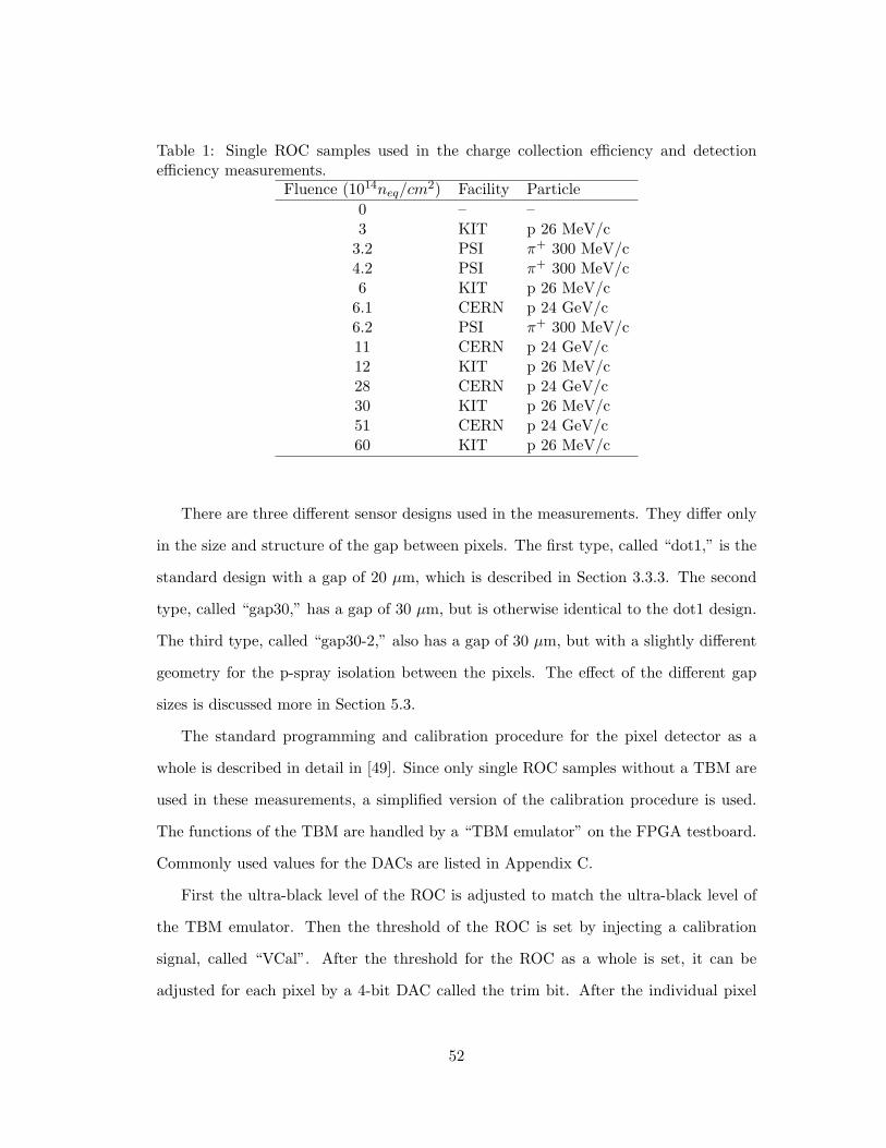
Table 1: Single ROC samples used in the charge collection efficiency and detectionefficiency measurements.
Fluence (1014neq/cm2) Facility Particle0 – –3 KIT p 26 MeV/c3.2 PSI π+ 300 MeV/c4.2 PSI π+ 300 MeV/c6 KIT p 26 MeV/c6.1 CERN p 24 GeV/c6.2 PSI π+ 300 MeV/c11 CERN p 24 GeV/c12 KIT p 26 MeV/c28 CERN p 24 GeV/c30 KIT p 26 MeV/c51 CERN p 24 GeV/c60 KIT p 26 MeV/c
There are three different sensor designs used in the measurements. They differ only
in the size and structure of the gap between pixels. The first type, called “dot1,” is the
standard design with a gap of 20 µm, which is described in Section 3.3.3. The second
type, called “gap30,” has a gap of 30 µm, but is otherwise identical to the dot1 design.
The third type, called “gap30-2,” also has a gap of 30 µm, but with a slightly different
geometry for the p-spray isolation between the pixels. The effect of the different gap
sizes is discussed more in Section 5.3.
The standard programming and calibration procedure for the pixel detector as a
whole is described in detail in [49]. Since only single ROC samples without a TBM are
used in these measurements, a simplified version of the calibration procedure is used.
The functions of the TBM are handled by a “TBM emulator” on the FPGA testboard.
Commonly used values for the DACs are listed in Appendix C.
First the ultra-black level of the ROC is adjusted to match the ultra-black level of
the TBM emulator. Then the threshold of the ROC is set by injecting a calibration
signal, called “VCal”. After the threshold for the ROC as a whole is set, it can be
adjusted for each pixel by a 4-bit DAC called the trim bit. After the individual pixel
52

thresholds have been adjusted, the response of the analog signal is calibrated versus the
VCal signal by injecting several different charge values. Finally, the pixel thresholds and
noise are measured with an “S-curve scan,” where the injected Vcal charge is adjusted
from 0 to the maximum value. The threshold is defined as the VCal value where the
efficiency is 50%, and the noise is the width of the associated Gaussian.
For the highly irradiated samples, some adjustments need to be made in the DAC val-
ues in order for the readout chip to function. For samples irradiated above 1015 neq/cm2
the preamplifier and shaper feedback circuit had to be adjusted, and the ADC sampling
point had to be shifted by a few nanoseconds. Commonly used DAC values for the
highly irradiated ROCs are also listed in Appendix C.
5.1 Charge Collection Efficiency
The charge collection efficiency of an irradiated sensor is defined as the ratio of amount of
charge collected from a MIP in the irradiated sensor compared to the amount of charge
collected from a MIP by an unirradiated detector. As a reference several unirradiated
sensors were tested under the same conditions as the irradiated sensors.
5.1.1 Testing Setup and Procedure
The testing setup consists of an insulated cold box, a sensor and ROC sample, a source,
and the electronics to read out the signal. The testing setup is shown in Figure 33. The
sample is mounted on an aluminum block inside the cold box, which is cooled by a water
cooled Peltier element. The box can be flushed with dry nitrogen to keep the humidity
as low as possible. Particles are provided by a 90Sr β source which is placed on a clear
plastic cap about 10 mm above the sensor. The endpoint energy of the β particles is
about 2.3 MeV, which pass through the sample and approximate a MIP. However there
are many low energy particles which are stopped in the sample and generate a much
larger signal. These low energy signals are reduced in the data analysis.
The ROC is controlled by an FPGA and custom written software. The read out
53

of the signal was triggered by a random trigger. Since the particles arrive randomly
in time, they are not synchronized with the randomly-generated trigger. Therefore the
clock cycle where the hits should arrive was stretched in order to increase the chances
that a particle passes through the sensor within the correct time window. The FPGA
stretches an arbitrary clock cycle to 1000 times the usual length. After a delay, a trigger
is sent to the ROC and the data from this stretched clock cycle is read out. The stretch
factor of 1000 was chosen such that approximately 80% of the triggers had hit pixels [50].
Later the setup was improved to contain a scintillator and photomultiplier tube
beneath the sample. The read out was then triggered by a coincidence of a signal
from the scintillator and the clock from the FPGA. The clock cycle stretching was not
necessary with the new setup, since the coincidence with the scintillator signal ensured
that a particle would pass through the detector during the correct clock cycle.
The sample is placed into the cold box and then cooled down to approximately -20C.
Once the temperature is stable, the standard programming and calibration procedure is
performed. After the working parameters have been optimized, a current-voltage (IV)
curve is taken for each sample to ensure that it is working properly. The bias voltage is
scanned through a range of values, starting from well below the depletion voltage, and
ending well into the depletion plateau. At each bias voltage value, data is collected for
15 seconds using the internal trigger.
5.1.2 Analysis
There are several steps in the analysis of the data. First some initial data quality cuts
are applied. Pixels can be manually excluded, which is usually done in the case of known
noisy pixels and the edge pixels, which are larger. In addition, there are several cuts
that can be used to exclude data from a pixel during the analysis of the data:
• The pixel has 10 times fewer hits than its neighbors.
• The pixel charge is very different compared to the charge of its neighbors.
54

Figure 33: Single sensor testing setup.
55
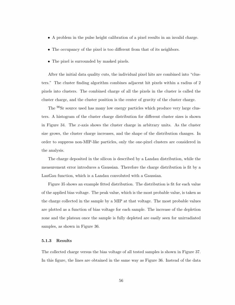
• A problem in the pulse height calibration of a pixel results in an invalid charge.
• The occupancy of the pixel is too different from that of its neighbors.
• The pixel is surrounded by masked pixels.
After the initial data quality cuts, the individual pixel hits are combined into “clus-
ters.” The cluster finding algorithm combines adjacent hit pixels within a radius of 2
pixels into clusters. The combined charge of all the pixels in the cluster is called the
cluster charge, and the cluster position is the center of gravity of the cluster charge.
The 90Sr source used has many low energy particles which produce very large clus-
ters. A histogram of the cluster charge distribution for different cluster sizes is shown
in Figure 34. The x-axis shows the cluster charge in arbitrary units. As the cluster
size grows, the cluster charge increases, and the shape of the distribution changes. In
order to suppress non-MIP-like particles, only the one-pixel clusters are considered in
the analysis.
The charge deposited in the silicon is described by a Landau distribution, while the
measurement error introduces a Gaussian. Therefore the charge distribution is fit by a
LanGau function, which is a Landau convoluted with a Gaussian.
Figure 35 shows an example fitted distribution. The distribution is fit for each value
of the applied bias voltage. The peak value, which is the most probable value, is taken as
the charge collected in the sample by a MIP at that voltage. The most probable values
are plotted as a function of bias voltage for each sample. The increase of the depletion
zone and the plateau once the sample is fully depleted are easily seen for unirradiated
samples, as shown in Figure 36.
5.1.3 Results
The collected charge versus the bias voltage of all tested samples is shown in Figure 37.
In this figure, the lines are obtained in the same way as Figure 36. Instead of the data
56
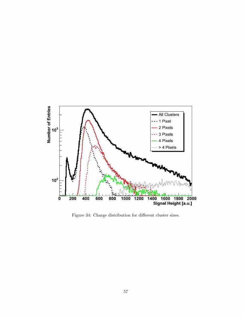
Figure 34: Charge distribution for different cluster sizes.
57
cQ1_923Entries 47758
Mean 381.1
RMS 107.3
/ ndf 2χ 200.3 / 73
Prob 8.526e-14
Width 0.37± 17.67
MP 0.4± 325.1
Area 1242± 2.431e+05
GSigma 0.53± 42.99
/65)-Charge (e0 500 1000 1500 2000
Entri
es
0
200
400
600
800
1000
1200
1400
1600
cQ1_923Entries 47758
Mean 381.1
RMS 107.3
/ ndf 2χ 200.3 / 73
Prob 8.526e-14
Width 0.37± 17.67
MP 0.4± 325.1
Area 1242± 2.431e+05
GSigma 0.53± 42.99
Charge Distribution for Clusters of 1 Pixels Run 923
Figure 35: Charge distribution for an unirradiated sample with a bias voltage of -150V fit by a LanGau function.
58

Figure 36: Charge vs bias voltage for an unirradiated sample.
59
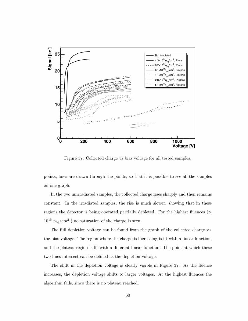
Voltage [V]0 200 400 600 800 1000
]-Si
gnal
[ke
0
5
10
15
20
25 Not irradiated
, Pions2/cmeqn1410×4.3, Pions2/cmeqn1410×6.2, Protons2/cmeqn1410×6.1, Protons2/cmeqn1510×1.1
, Protons2/cmeqn1510×2.8, Protons2/cmeqn1510×5.1
Figure 37: Collected charge vs bias voltage for all tested samples.
points, lines are drawn through the points, so that it is possible to see all the samples
on one graph.
In the two unirradiated samples, the collected charge rises sharply and then remains
constant. In the irradiated samples, the rise is much slower, showing that in these
regions the detector is being operated partially depleted. For the highest fluences (>
1015 neq/cm2 ) no saturation of the charge is seen.
The full depletion voltage can be found from the graph of the collected charge vs.
the bias voltage. The region where the charge is increasing is fit with a linear function,
and the plateau region is fit with a different linear function. The point at which these
two lines intersect can be defined as the depletion voltage.
The shift in the depletion voltage is clearly visible in Figure 37. As the fluence
increases, the depletion voltage shifts to larger voltages. At the highest fluences the
algorithm fails, since there is no plateau reached.
60

Columns0 10 20 30 40 50
Row
s
0
10
20
30
40
50
60
70
80
0
20
40
60
80
100
120
140
Pixel Occupancy
Figure 38: Two dimensional map of hits within the sample irradiated to 5×10¹⁵ neq/cm2.The distinctive “bulls-eye” pattern of a point source is clearly visible, indicating thatthe signals are produced by actual particles and not noise.
Only two samples irradiated to 5×10¹⁵ neq/cm2 were able to be tested. The amount
of charge shown for these samples in Figure 37 is at the nominal threshold level, and
does not seem to change with bias voltage. We believe that the threshold is in the tail
of the Landau distribution, giving a wrong value for the amount of charge collected.
The most probable value of the distribution is then always at the threshold, and does
not depend on the bias voltage.
However, by looking at the two dimensional map of the signals versus position in
the sensor (Figure 38), it is obvious that the signals are produced by real particles from
the 90Sr source crossing the sensor. Particles coming from a point source such as the
90Sr source produce a distinctive “bulls-eye” pattern, while noise produces a uniform
distribution.
61
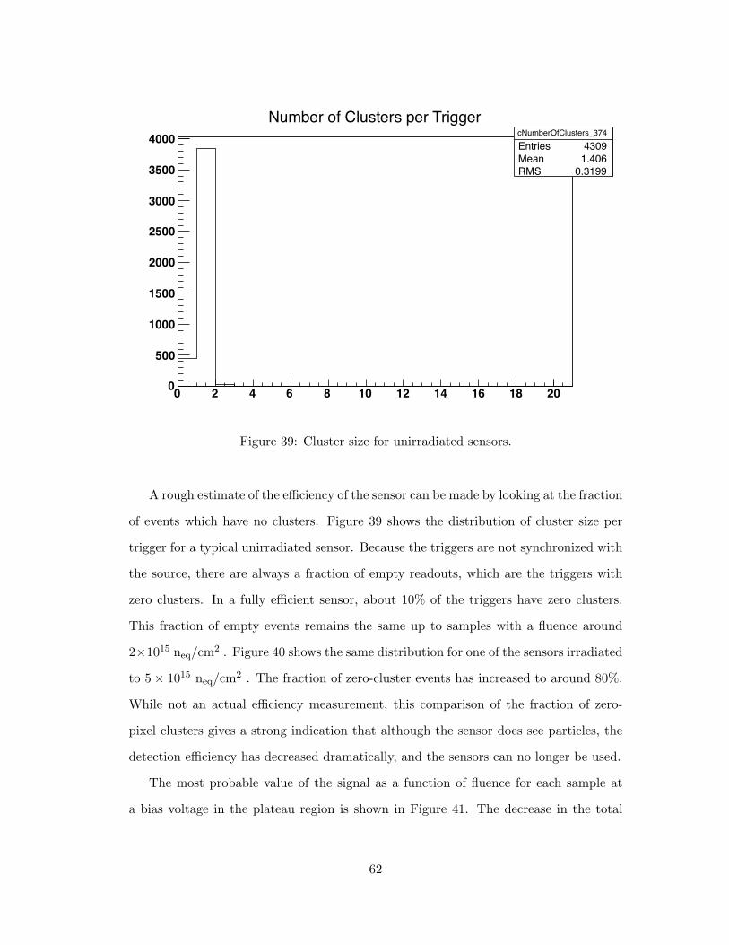
cNumberOfClusters_374Entries 4309Mean 1.406RMS 0.3199
0 2 4 6 8 10 12 14 16 18 200
500
1000
1500
2000
2500
3000
3500
4000 cNumberOfClusters_374Entries 4309Mean 1.406RMS 0.3199
Number of Clusters per Trigger
Figure 39: Cluster size for unirradiated sensors.
A rough estimate of the efficiency of the sensor can be made by looking at the fraction
of events which have no clusters. Figure 39 shows the distribution of cluster size per
trigger for a typical unirradiated sensor. Because the triggers are not synchronized with
the source, there are always a fraction of empty readouts, which are the triggers with
zero clusters. In a fully efficient sensor, about 10% of the triggers have zero clusters.
This fraction of empty events remains the same up to samples with a fluence around
2×10¹⁵ neq/cm2 . Figure 40 shows the same distribution for one of the sensors irradiated
to 5× 10¹⁵ neq/cm2 . The fraction of zero-cluster events has increased to around 80%.
While not an actual efficiency measurement, this comparison of the fraction of zero-
pixel clusters gives a strong indication that although the sensor does see particles, the
detection efficiency has decreased dramatically, and the sensors can no longer be used.
The most probable value of the signal as a function of fluence for each sample at
a bias voltage in the plateau region is shown in Figure 41. The decrease in the total
62
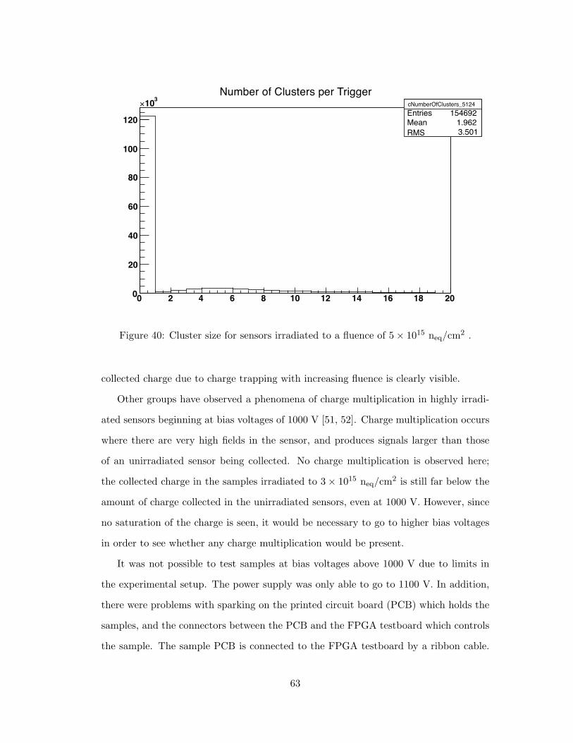
cNumberOfClusters_5124Entries 154692Mean 1.962RMS 3.501
0 2 4 6 8 10 12 14 16 18 200
20
40
60
80
100
120
310× cNumberOfClusters_5124Entries 154692Mean 1.962RMS 3.501
Number of Clusters per Trigger
Figure 40: Cluster size for sensors irradiated to a fluence of 5× 10¹⁵ neq/cm2 .
collected charge due to charge trapping with increasing fluence is clearly visible.
Other groups have observed a phenomena of charge multiplication in highly irradi-
ated sensors beginning at bias voltages of 1000 V [51, 52]. Charge multiplication occurs
where there are very high fields in the sensor, and produces signals larger than those
of an unirradiated sensor being collected. No charge multiplication is observed here;
the collected charge in the samples irradiated to 3× 10¹⁵ neq/cm2 is still far below the
amount of charge collected in the unirradiated sensors, even at 1000 V. However, since
no saturation of the charge is seen, it would be necessary to go to higher bias voltages
in order to see whether any charge multiplication would be present.
It was not possible to test samples at bias voltages above 1000 V due to limits in
the experimental setup. The power supply was only able to go to 1100 V. In addition,
there were problems with sparking on the printed circuit board (PCB) which holds the
samples, and the connectors between the PCB and the FPGA testboard which controls
the sample. The sample PCB is connected to the FPGA testboard by a ribbon cable.
63
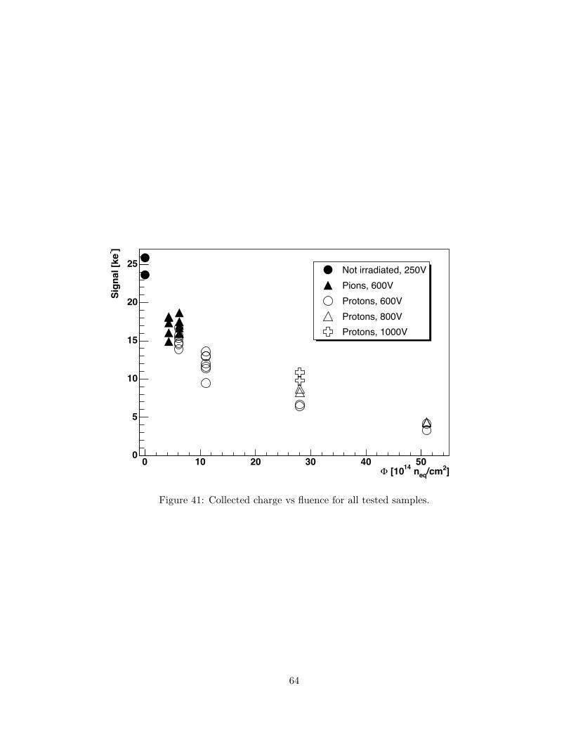
]2/cmeq n14 [10Φ0 10 20 30 40 50
]-Si
gnal
[ke
0
5
10
15
20
25 Not irradiated, 250VPions, 600VProtons, 600VProtons, 800VProtons, 1000V
Figure 41: Collected charge vs fluence for all tested samples.
64
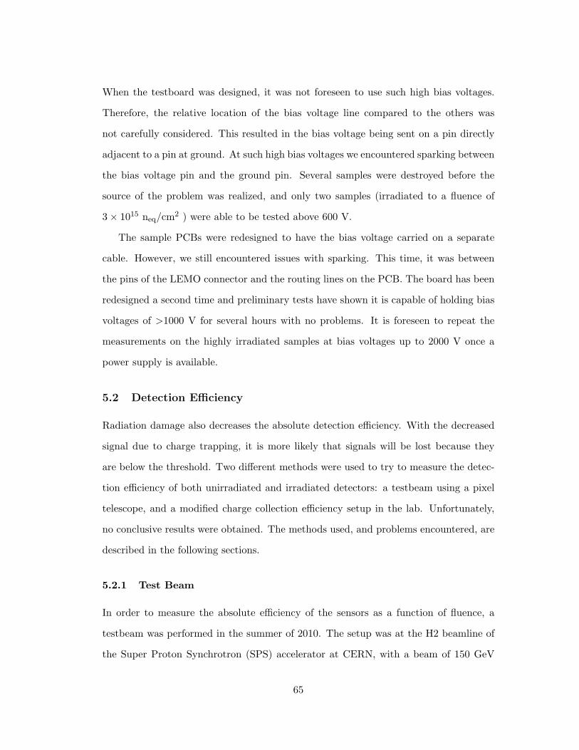
When the testboard was designed, it was not foreseen to use such high bias voltages.
Therefore, the relative location of the bias voltage line compared to the others was
not carefully considered. This resulted in the bias voltage being sent on a pin directly
adjacent to a pin at ground. At such high bias voltages we encountered sparking between
the bias voltage pin and the ground pin. Several samples were destroyed before the
source of the problem was realized, and only two samples (irradiated to a fluence of
3× 10¹⁵ neq/cm2 ) were able to be tested above 600 V.
The sample PCBs were redesigned to have the bias voltage carried on a separate
cable. However, we still encountered issues with sparking. This time, it was between
the pins of the LEMO connector and the routing lines on the PCB. The board has been
redesigned a second time and preliminary tests have shown it is capable of holding bias
voltages of >1000 V for several hours with no problems. It is foreseen to repeat the
measurements on the highly irradiated samples at bias voltages up to 2000 V once a
power supply is available.
5.2 Detection Efficiency
Radiation damage also decreases the absolute detection efficiency. With the decreased
signal due to charge trapping, it is more likely that signals will be lost because they
are below the threshold. Two different methods were used to try to measure the detec-
tion efficiency of both unirradiated and irradiated detectors: a testbeam using a pixel
telescope, and a modified charge collection efficiency setup in the lab. Unfortunately,
no conclusive results were obtained. The methods used, and problems encountered, are
described in the following sections.
5.2.1 Test Beam
In order to measure the absolute efficiency of the sensors as a function of fluence, a
testbeam was performed in the summer of 2010. The setup was at the H2 beamline of
the Super Proton Synchrotron (SPS) accelerator at CERN, with a beam of 150 GeV
65

pions [53]. The setup consisted of a telescope of 4 pixel sensors, an independent trigger
consisting of a silicon diode, and the device under test (DUT) in the center. The
telescope chips were small CMS pixel sensors bump-bonded to a single ROC. They were
identical to the DUT, except that they were not irradiated. A diagram of the telescope
is shown in Figure 42. This setup was placed between a pair of Helmholtz coils which
produced a 3 T magnetic field, in order to also measure the change in the Lorentz angle
as a function of fluence.
The DUT was placed inside an insulated cold box, so that the irradiated sensors
could be tested at a temperature of -10C. The sample was cooled by two Peltier coolers.
The heat was removed from the Peltier coolers by cooling fluid, which passed through
a chiller placed outside the beam area.
The FPGA testboard which controlled the telescope and DUT was placed inside the
magnet below the telescope. All of the other controlling electronics (power supplies,
triggering electronics, data acquisition computers) were placed outside of the beam area
so that they could be easily accessed during the beam operation.
The readout of the telescope required an external trigger. The trigger consisted of a
standard CMS barrel pixel silicon sensor, which was not bump bonded to a ROC. The
charge was read out using a fast commercial amplifier and discriminator wirebonded
to the back side of the sensor. The threshold and width of the signal pulse could be
adjusted by two potentiometers on the trigger board. The trigger was controlled by
standard Nuclear Instrumentation Module (NIM) electronics, located in the control
room. The trigger board is shown in Figure 43.
The telescope and DUT were controlled by a modified version of the software used
in the characterization and testing of modules before they were installed in CMS. The
telescope and DUT are considered a “module” consisting of only 5 ROCs. The telescope
chips and the DUT were programmed and calibrated using the standard calibration
procedure, and data taking followed the same procedure as for the charge collection
efficiency measurements.
66

Figure 42: Top: Diagram of the pixel telescope used at the testbeam, showing thelocation of the device under test. Bottom: Photograph of the pixel telescope.
67

Figure 43: Photograph of the trigger board. The sensor is under the foil cap.
68
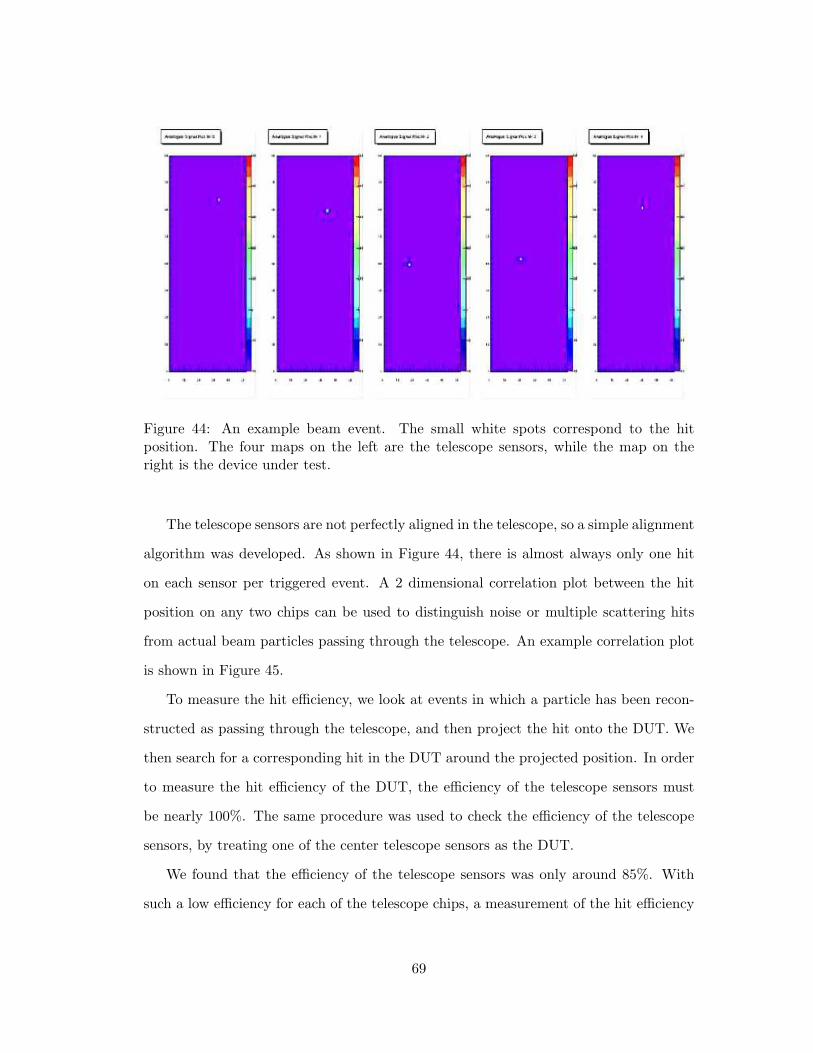
Figure 44: An example beam event. The small white spots correspond to the hitposition. The four maps on the left are the telescope sensors, while the map on theright is the device under test.
The telescope sensors are not perfectly aligned in the telescope, so a simple alignment
algorithm was developed. As shown in Figure 44, there is almost always only one hit
on each sensor per triggered event. A 2 dimensional correlation plot between the hit
position on any two chips can be used to distinguish noise or multiple scattering hits
from actual beam particles passing through the telescope. An example correlation plot
is shown in Figure 45.
To measure the hit efficiency, we look at events in which a particle has been recon-
structed as passing through the telescope, and then project the hit onto the DUT. We
then search for a corresponding hit in the DUT around the projected position. In order
to measure the hit efficiency of the DUT, the efficiency of the telescope sensors must
be nearly 100%. The same procedure was used to check the efficiency of the telescope
sensors, by treating one of the center telescope sensors as the DUT.
We found that the efficiency of the telescope sensors was only around 85%. With
such a low efficiency for each of the telescope chips, a measurement of the hit efficiency
69
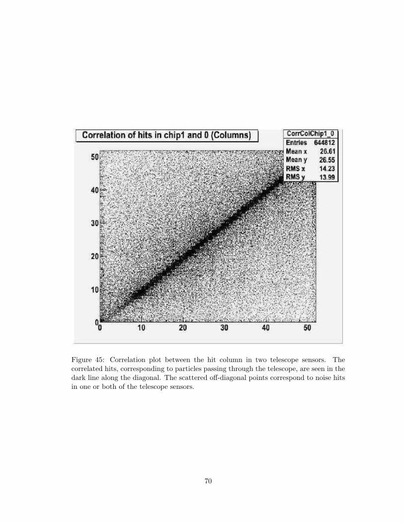
Figure 45: Correlation plot between the hit column in two telescope sensors. Thecorrelated hits, corresponding to particles passing through the telescope, are seen in thedark line along the diagonal. The scattered off-diagonal points correspond to noise hitsin one or both of the telescope sensors.
70

Figure 46: Illustration of timewalk. Low amplitude signals cross threshold late and areassigned to the wrong bunch crossing.
in the DUT is impossible, as the expected effects are on the order of a few percent.
The low efficiency appears to be due to a timing problem. In the LHC, the clock of the
pixel detector is synchronized to the beam. However, at the testbeam the clock is not
synchronized. This leads to two possible timing problems: triggers arriving too late in
the bunch crossing, and timewalk.
The timewalk problem is illustrated in Figure 46. Low amplitude signals reach the
threshold later than high amplitude signals. This leads to the effect that a low amplitude
signal may not cross the threshold in the correct bunch crossing. By using the right
delays, this problem is neglible in events where the clock is synchronized to the beam.
In the case of an unsynchronized beam, the particles may arrive too late in the time
window for low amplitude signals to cross the threshold in time. Then the “in-time
threshold” can be defined as the minimum amplitude a signal would need in order to
cross the absolute threshold within the bunch crossing.
The other timing problem occurs when triggers arrive too late in the bunch crossing,
71
so the signal does not cross the threshold until the next bunch crossing. These particles
are then “lost”. In addition, the timing can be slightly different between the different
chips of the telescope and the DUT. This means that it is impossible to tell whether a
particle which is seen in the telescope but not in the DUT was lost due to this timing
effect or a decrease in the sensor efficiency.
In order to avoid these problems and achieve an acceptable efficiency for the tele-
scope, a very small time window for accepting triggers is necessary. This problem will
be solved in future test beams.
5.2.2 Lab Setup
The testing setup used in the charge collection efficiency measurements was modified to
have an independent trigger by adding a scintillator and photomultiplier tube beneath
the sample. A diagram of the setup is shown in Figure 47. The testboard was triggered
by a coincidence of a signal from the scintillator and the rising edge of the testboard
clock. A photograph of the setup is shown in Figure 48.
The procedure foreseen for the efficiency measurements is the same as for the charge
collection efficiency measurements. The sample is placed into the cold box and cooled
to -20C, the programming and calibration procedure is performed, and an IV curve is
taken to assess the quality of the sample. After that data is taken for 15 seconds at
a bias voltage slightly above the depletion voltage. The detection efficiency is defined
as the number of triggered readouts with hits divided by the total number of triggered
readouts.
To verify the procedure, the measurement was first performed with an unirradiated
sample. The efficiency of the unirradiated sensors has been previously measured, and
found to be greater than 99% [54]. However, when testing the efficiency of the unirra-
diated sensors in the lab setup, the measured efficiency was much lower than expected.
It is thought that this is due to multiple scattering of the β particles inside the box.
In order to mitigate this effect, lead shielding was added to narrow the available path
72
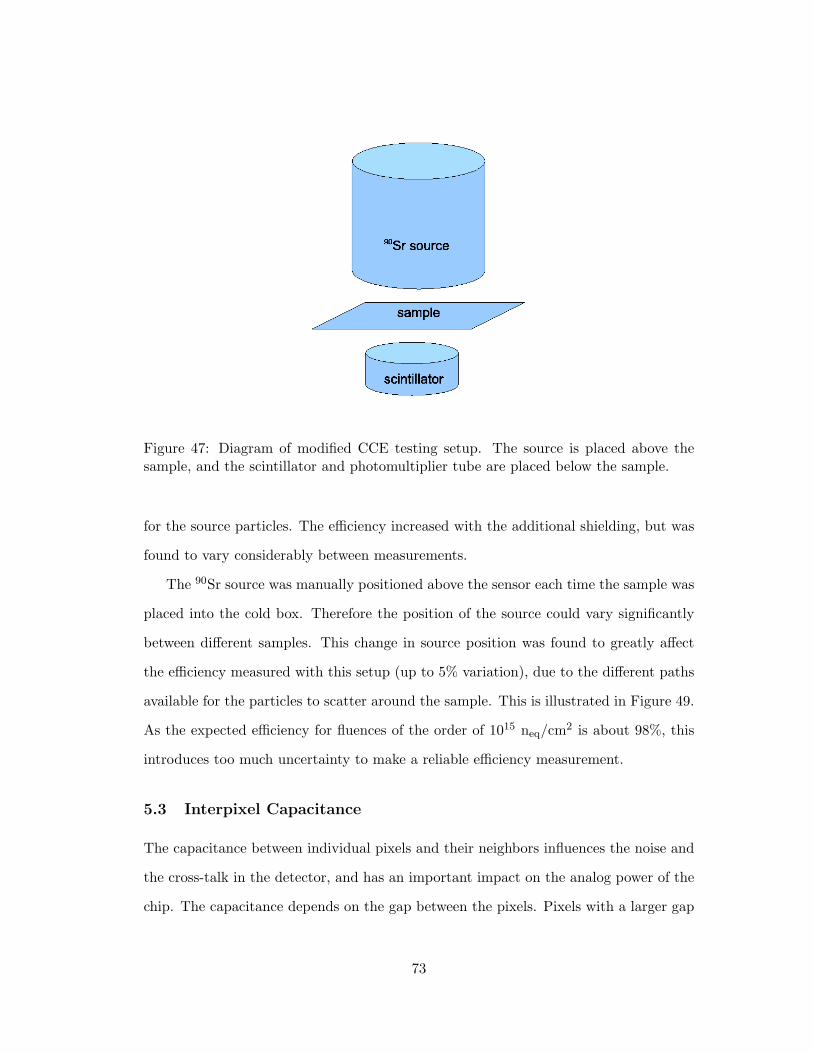
Figure 47: Diagram of modified CCE testing setup. The source is placed above thesample, and the scintillator and photomultiplier tube are placed below the sample.
for the source particles. The efficiency increased with the additional shielding, but was
found to vary considerably between measurements.
The 90Sr source was manually positioned above the sensor each time the sample was
placed into the cold box. Therefore the position of the source could vary significantly
between different samples. This change in source position was found to greatly affect
the efficiency measured with this setup (up to 5% variation), due to the different paths
available for the particles to scatter around the sample. This is illustrated in Figure 49.
As the expected efficiency for fluences of the order of 1015 neq/cm2 is about 98%, this
introduces too much uncertainty to make a reliable efficiency measurement.
5.3 Interpixel Capacitance
The capacitance between individual pixels and their neighbors influences the noise and
the cross-talk in the detector, and has an important impact on the analog power of the
chip. The capacitance depends on the gap between the pixels. Pixels with a larger gap
73
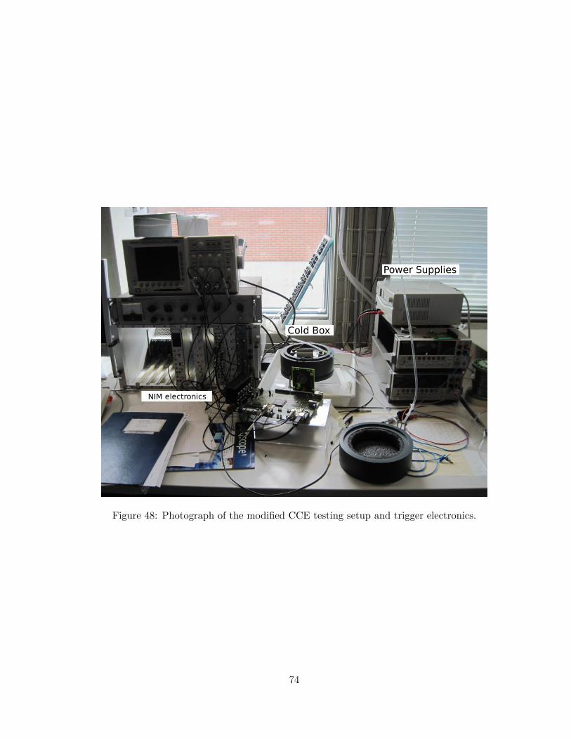
Figure 48: Photograph of the modified CCE testing setup and trigger electronics.
74

Figure 49: Diagram showing how the source position affects the efficiency. Differentsource positions provide different paths for the scattered particles.
75

size have a smaller interpixel capacitance, but the larger gaps produce an inhomogenous
drift field inside the sensor. Therefore it is important to find a balance between the
capacitance and the gap size.
The current CMS barrel pixel sensors have small gaps (20 µm), and accordingly
a relatively high interpixel capacitance. In order to test whether reducing the inter-
pixel capacitance by increasing the gap size would be beneficial, several samples were
produced with a gap size of 30 µm, typically referred to as “gap-30”. The interpixel
capacitance is measured as a function of bias voltage for both the standard and gap-30
samples. The samples are then irradiated with a 60Co source and then measured again.
The measurements are described in Section 5.3.1
A first attempt was made at simulating the interpixel capacitance using a Synopsis
TCAD simulation [55]. The results can be qualitatively compared with the results of
the measurements. The simulation is described in Section 5.3.2.
5.3.1 Measurements
The small value of the capacitance, combined with the small pixel size, makes mea-
suring the interpixel capacitance a challenge. A new method to measure the interpixel
capacitance was developed, where a simple chip is bump bonded onto the sensor instead
of the ROC. This chip is referred to as the “readout replacement chip.”
The concept of the measurement method is to form a basic unit cell of one pixel
surrounded by the eight directly neighboring pixels. The eight neighboring pixels are
connected together. Then the capacitance can be measured between the central pixel
and the eight connected neighbor pixels. A picture of this basic unit cell is shown in
Figure 50. This basic unit is repeated over the entire chip. The central pixel of each cell
is connected together and routed to a pad on the edge of the chip. The eight neighbor
pixels of each cell are also connected together over the whole chip and routed to a second
pad on the edge of the chip. These two pads can be contacted with a needle, and the
capacitance can be measured. The measurement setup is shown in Figure 51.
76
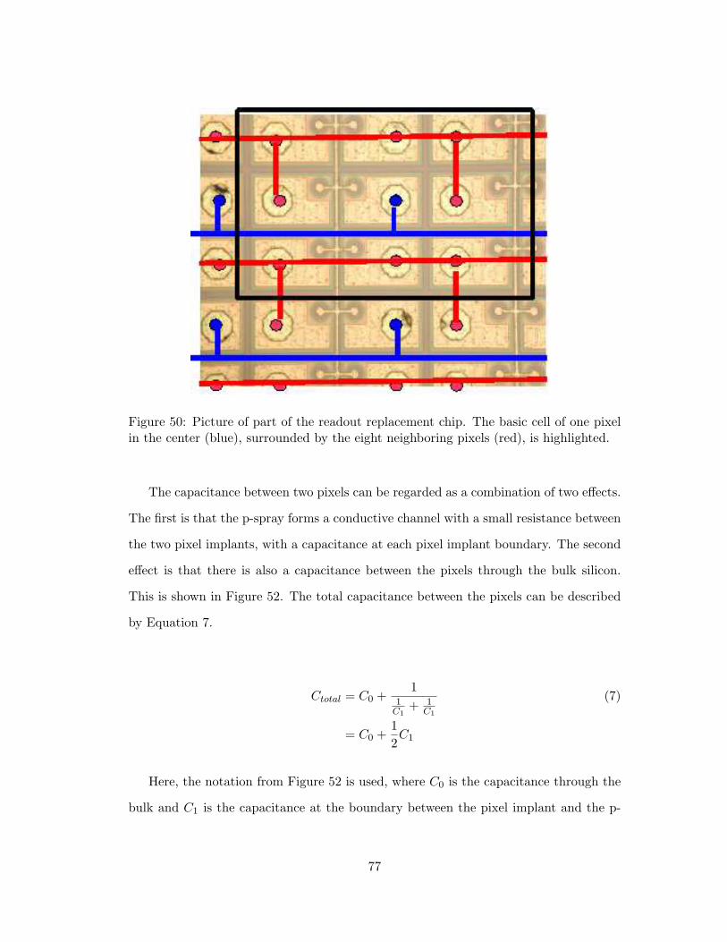
Figure 50: Picture of part of the readout replacement chip. The basic cell of one pixelin the center (blue), surrounded by the eight neighboring pixels (red), is highlighted.
The capacitance between two pixels can be regarded as a combination of two effects.
The first is that the p-spray forms a conductive channel with a small resistance between
the two pixel implants, with a capacitance at each pixel implant boundary. The second
effect is that there is also a capacitance between the pixels through the bulk silicon.
This is shown in Figure 52. The total capacitance between the pixels can be described
by Equation 7.
Ctotal = C0 +1
1C1
+ 1C1
(7)
= C0 +1
2C1
Here, the notation from Figure 52 is used, where C0 is the capacitance through the
bulk and C1 is the capacitance at the boundary between the pixel implant and the p-
77

Figure 51: The interpixel capacitance measurement setup.
78

Figure 52: Diagram of interpixel capacitance. C0 represents the capacitance betweenpixels through the bulk, C1 represents the capacitance between the pixel implant andthe p-spray, and R represents the resistance of the p-spray.
79

spray. As the bias voltage increases, the p-spray begins to be depleted of charge carriers,
the resistance R increases, and the capacitance between the pixel implant and the p-
spray (C1) decreases. Eventually, the contribution of the C1 term to the capacitance
becomes negligible, and the capacitance approaches the value of C0.
Because the interpixel capacitance depends mostly on surface effects, the surface
damage caused by radiation is important, while the bulk damage has little to no effect.
Therefore some of the samples were irradiated at PSI with a 60Co gamma source with
a dose of 20 kGy. At this dose the fixed surface charge should be saturated [56].
The samples are listed in Table 2. One sample of each type was measured before
and after irradiation.
Table 2: Samples used in the interpixel capacitance measurements and the measuredcapacitance at a bias voltage of 150 V. Errors are discussed in the text.
Sample Number Type Gap Size (µm) Capacitance (fF)8609-02-11 Gap20 20 1008609-02-12 Gap20 20 658609-02-10 Gap30 30 208609-02-13 Gap30-2 30 508609-02-14 Gap30-3 30 858609-18-06 Gap20 20 1008609-18-07 Gap20 20 558609-18-05 Gap30 30 658609-18-08 Gap30-2 30 308609-18-09 Gap30-3 30 45271947-18-11 Gap20 20 70271947-18-12 Gap20 20 105271947-18-10 Gap30 30 45271947-18-13 Gap30-2 30 45271947-18-14 Gap30-3 30 45
The main source for errors in these measurements comes from the measurement of
the stray capacitance of the readout replacement chip. To measure this capacitance,
the sample must be removed from the setup, the readout replacement chip must be
forcibly removed from the sensor, and then the readout replacement chip is placed back
into the setup to be measured alone. This process can change something on the chip,
80
for instance smear the bump bonds, or the contact resistances might be changed by
putting the readout replacement chip in a slightly different position. The best way
to estimate the size of the errors introduced here is to compare the measurements of
identical samples.
There are two samples from each wafer of the gap20 type, which are shown in
Table 2. For samples 8609-02-11 and 8609-02-12, the measured capacitances are 100 fF
and 65 fF, respectively, with a difference of 35 fF between the two measurements. For
samples 8609-18-06 and 8609-18-07, the measured capacitances are 100 fF and 55 fF,
respectively, with a difference of 45 fF. For samples 271947-18-11 and 271947-18-12 the
measured capacitances are 70 fF and 105 fF, respectively, with a difference of 35 fF. The
average difference between identical samples is 38 fF, so 40 fF is taken as the uncertainty
on the measurements.
The results of the interpixel capacitance measurements before irradiation are shown
in Figure 53. Before full depletion, the pixels are not isolated from each other. The
relevant part of the curve is the part from the full depletion voltage onwards, which can
easily be seen by the sharp spike around 50 V. After the full depletion, the capacitance
decreases with increasing voltage until a plateau is reached.
The results of the measurements of the irradiated samples are shown in Figure 54.
The solid lines are the measurements of the samples before irradiation, and the dashed
lines are the measurements of the samples after irradiation. The capacitance of the gap-
30 samples is indeed lower than the capacitance of the standard samples. The interpixel
capacitance after irradiation is lower than before irradiation. This is likely due to the
build up of positive charges along the surface after irradiation. This layer of positive
charges begins the depletion of the p-spray earlier than in the unirradiated samples, so
the capacitance decreases faster.
81
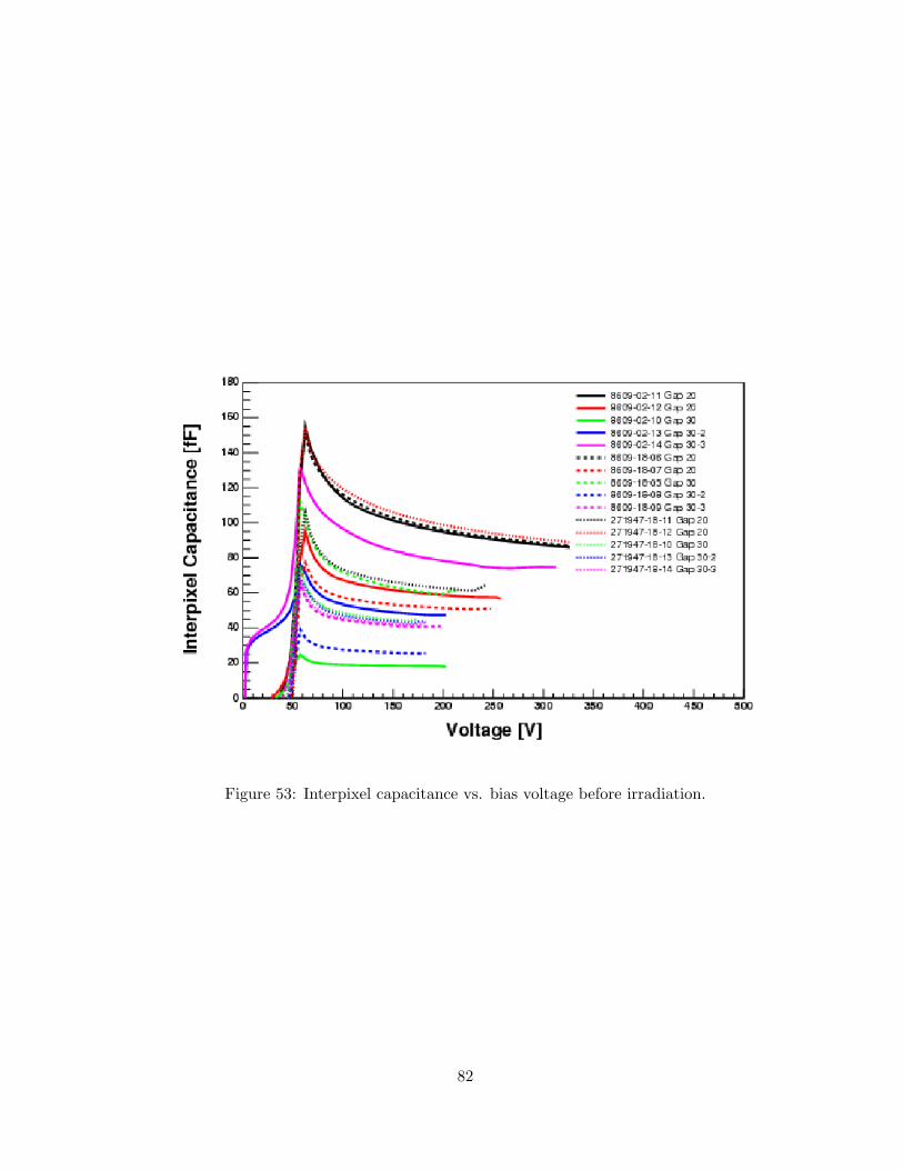
Figure 53: Interpixel capacitance vs. bias voltage before irradiation.
82
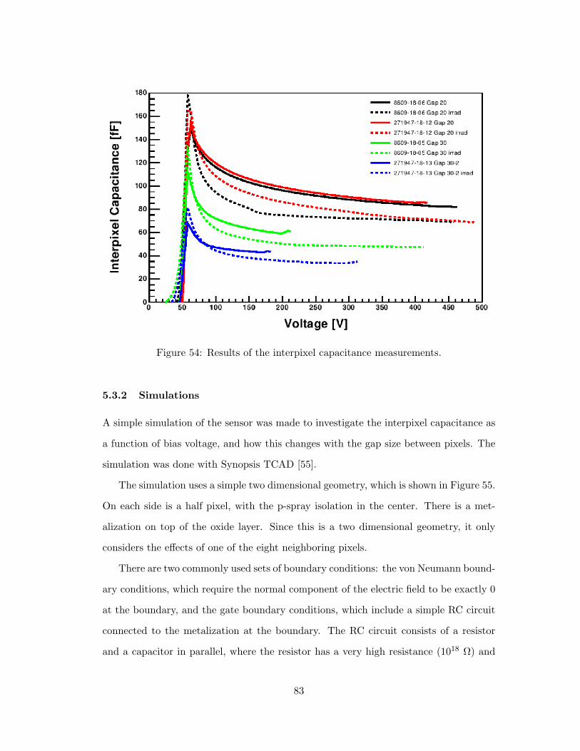
Figure 54: Results of the interpixel capacitance measurements.
5.3.2 Simulations
A simple simulation of the sensor was made to investigate the interpixel capacitance as
a function of bias voltage, and how this changes with the gap size between pixels. The
simulation was done with Synopsis TCAD [55].
The simulation uses a simple two dimensional geometry, which is shown in Figure 55.
On each side is a half pixel, with the p-spray isolation in the center. There is a met-
alization on top of the oxide layer. Since this is a two dimensional geometry, it only
considers the effects of one of the eight neighboring pixels.
There are two commonly used sets of boundary conditions: the von Neumann bound-
ary conditions, which require the normal component of the electric field to be exactly 0
at the boundary, and the gate boundary conditions, which include a simple RC circuit
connected to the metalization at the boundary. The RC circuit consists of a resistor
and a capacitor in parallel, where the resistor has a very high resistance (1018 Ω) and
83

Figure 55: The geometry and doping profile of the simulated sensor area.
84

the capacitor has a very low capacitance (10−18 F). Requiring the potential to be zero
at the boundary represents the situation in vacuum, and creates high fields inside the
sensor. Our measurements are performed in a normal ambient environment, so the gate
boundary conditions represent a more realistic picture of the measurement environment
and fields inside the sensor.
The gate boundary conditions are a better reflection of the environment, since our
measurements are not performed in vacuum, and so the simulations are done with
the gate boundary conditions. The capacitances to be simulated are very small, and
a small signal analysis tends to have convergence problems. The best convergence
with the gate boundary conditions is given by indirectly simulating the capacitance by
injecting a voltage into the pixel and measuring the induced current. The capacitance
is proportional to the induced current, as shown in Equation 8, where Q is the charge,
C is the capacitance, and V is the potential, and dQdt = I is the current.
Q ∝ CV (8)
dQ
dt∝ C
dV
dt
C ∝IdVdt
The simulation is run using three different gap sizes: 20 µm, 30 µm, and an extreme
case of 50 µm. The current for each of these is shown in Figure 56. As expected, the
current decreases with increasing gap size.
This simulation is greatly simplified and can not be compared quantitatively with
the measurements. Many other effects are not considered here, such as the effect of the
corner pixels. However, a qualitative comparison can be made. The general trend of
the measurements is fairly well reproduced, with the current decreasing with increasing
bias voltage, although the simulation underestimates the reduction of the capacitance
with increasing bias voltage.
85

Figure 56: The current induced in the gate as a function of bias voltage in the simulationfor different gap sizes.
5.4 High Voltage Tests on Single Sided Sensors
Single-sided sensors offer a cheaper alternative to double-sided processed sensors. Pre-
vious tests have shown them to have equivalent radiation hardness to double-sided
sensors [57]. However the single side processing does not allow a guard ring structure
on the back side of the sensor. This leaves the edges of the sensor at high voltage, while
the ROC is at ground, as shown in Figure 57. There is nothing between the sensor and
the ROC besides air. Air has a breakdown electric field of ∼3 V/µm. The distance
between the sensor and the ROC depends on the bump bonding process, but is on the
order of 10’s of µm. In the case of the CMS pixels, the distance between the sensor
and the ROC is 20 µm. When a bias voltage of a few hundred Volts is applied to the
sensor there is a non-negligible chance of sparking between the ROC and the sensor. In
order for single sided sensors to be a viable alternative to the more expensive double
sided sensors, there must be an inexpensive and easily scalable solution to the sparking
problem.
86
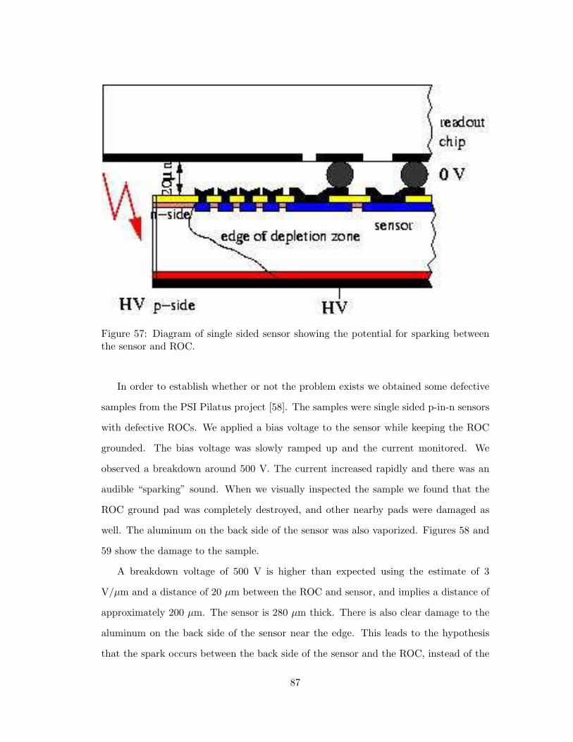
Figure 57: Diagram of single sided sensor showing the potential for sparking betweenthe sensor and ROC.
In order to establish whether or not the problem exists we obtained some defective
samples from the PSI Pilatus project [58]. The samples were single sided p-in-n sensors
with defective ROCs. We applied a bias voltage to the sensor while keeping the ROC
grounded. The bias voltage was slowly ramped up and the current monitored. We
observed a breakdown around 500 V. The current increased rapidly and there was an
audible “sparking” sound. When we visually inspected the sample we found that the
ROC ground pad was completely destroyed, and other nearby pads were damaged as
well. The aluminum on the back side of the sensor was also vaporized. Figures 58 and
59 show the damage to the sample.
A breakdown voltage of 500 V is higher than expected using the estimate of 3
V/µm and a distance of 20 µm between the ROC and sensor, and implies a distance of
approximately 200 µm. The sensor is 280 µm thick. There is also clear damage to the
aluminum on the back side of the sensor near the edge. This leads to the hypothesis
that the spark occurs between the back side of the sensor and the ROC, instead of the
87
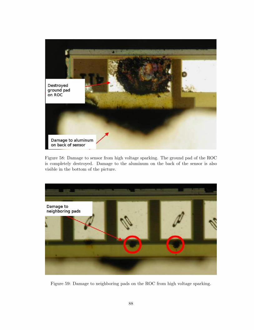
Figure 58: Damage to sensor from high voltage sparking. The ground pad of the ROCis completely destroyed. Damage to the aluminum on the back of the sensor is alsovisible in the bottom of the picture.
Figure 59: Damage to neighboring pads on the ROC from high voltage sparking.
88
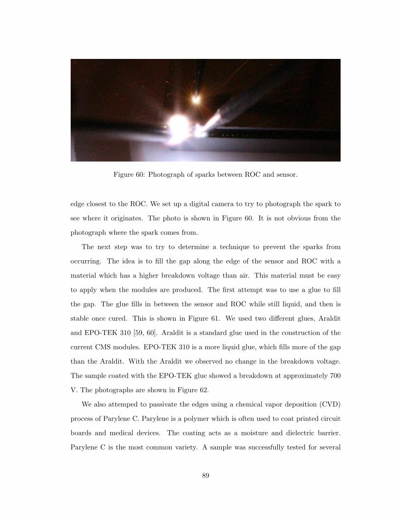
Figure 60: Photograph of sparks between ROC and sensor.
edge closest to the ROC. We set up a digital camera to try to photograph the spark to
see where it originates. The photo is shown in Figure 60. It is not obvious from the
photograph where the spark comes from.
The next step was to try to determine a technique to prevent the sparks from
occurring. The idea is to fill the gap along the edge of the sensor and ROC with a
material which has a higher breakdown voltage than air. This material must be easy
to apply when the modules are produced. The first attempt was to use a glue to fill
the gap. The glue fills in between the sensor and ROC while still liquid, and then is
stable once cured. This is shown in Figure 61. We used two different glues, Araldit
and EPO-TEK 310 [59, 60]. Araldit is a standard glue used in the construction of the
current CMS modules. EPO-TEK 310 is a more liquid glue, which fills more of the gap
than the Araldit. With the Araldit we observed no change in the breakdown voltage.
The sample coated with the EPO-TEK glue showed a breakdown at approximately 700
V. The photographs are shown in Figure 62.
We also attemped to passivate the edges using a chemical vapor deposition (CVD)
process of Parylene C. Parylene is a polymer which is often used to coat printed circuit
boards and medical devices. The coating acts as a moisture and dielectric barrier.
Parylene C is the most common variety. A sample was successfully tested for several
89

Figure 61: Diagram of single sided sensor using glue to fill the edge gap between thesensor and the ROC.
90

Figure 62: Damage to sensors with glue filled gaps.
91
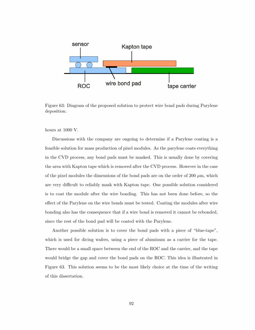
Figure 63: Diagram of the proposed solution to protect wire bond pads during Parylenedeposition.
hours at 1000 V.
Discussions with the company are ongoing to determine if a Parylene coating is a
feasible solution for mass production of pixel modules. As the parylene coats everything
in the CVD process, any bond pads must be masked. This is usually done by covering
the area with Kapton tape which is removed after the CVD process. However in the case
of the pixel modules the dimensions of the bond pads are on the order of 200 µm, which
are very difficult to reliably mask with Kapton tape. One possible solution considered
is to coat the module after the wire bonding. This has not been done before, so the
effect of the Parylene on the wire bonds must be tested. Coating the modules after wire
bonding also has the consequence that if a wire bond is removed it cannot be rebonded,
since the rest of the bond pad will be coated with the Parylene.
Another possible solution is to cover the bond pads with a piece of “blue-tape”,
which is used for dicing wafers, using a piece of aluminum as a carrier for the tape.
There would be a small space between the end of the ROC and the carrier, and the tape
would bridge the gap and cover the bond pads on the ROC. This idea is illustrated in
Figure 63. This solution seems to be the most likely choice at the time of the writing
of this dissertation.
92
6 b Production
6.1 Theory
Measurements of heavy flavor quark production at hadron colliders provide a good test
of quantum chromodynamics (QCD) [61]. The leading order (LO) process for b quark
production at hadron colliders is flavor creation, where a bb pair is produced by quark-
antiquark annihilation or gluon-gluon fusion. Since the final state is a two-body state,
the b quarks are usually produced back-to-back and with balanced pT.
At the LHC next to leading order (NLO) processes become important. In flavor
excitation, a bb pair from the quark sea of one proton is excited into the final state,
after one of the quarks undergoes a hard scattering off a parton from the other proton.
Because only one of the final quarks was involved in the hard scattering process, the b
quarks can be produced with asymmetric pT . In gluon splitting, a gluon in either the
initial or final state splits into a bb pair. Neither quark is involved in the hard scattering,
and the bb pair can be produced with a small angular separation. Figure 64 shows the
Feynmann diagrams for these processes. The small-x effects (x - mb/√s) are relevant
in the low-pT domain [62, 63], while multiple gluon radiation is more imporant at high
pT [64]. Measurements which help to discriminate effects in different pT and η regions
are needed to test the calculations.
6.2 Monte Carlo Event Generators
The measurements are often compared with theoretical predictions. This is generally
done using Monte Carlo event generators, which allow an event-by-event prediction of
the QCD processes. The first step in the event generation is to calculate the matrix
element with pQCD. Next a parton shower algorithm is run to generate the secondary
partons, followed by a hadronization algorithm, which groups the partons into hadrons.
Two common codes for computing these predictions at next-to-leading order are the
Monte Carlo for FeMtobarn processes (MCFM) [65] and the Fixed Order plus Next-to-
93

(a) Flavor creation (b) Flavor excitation
(c) Gluon splitting
Figure 64: Examples of the LO and NLO processes for heavy quark production athadron colliders. [11]
Leading Logarithm (FONLL) [66]. The MCFM code is a NLO calculation, while the
FONLL code is, as the name suggests, a NLO calculation including the resummation of
pT logarithms to next-to-leading order. Other common leading order event generators
are PYTHIA [67] and Herwig [68]. In PYTHIA and Herwig, the matrix elements are
calculated using leading-order pQCD. There are a few ways to extend the LO event
generators to include NLO corrections. MC@NLO is a package which combines the
LO Herwig event generator with NLO calculations of rates of QCD processes [69, 70].
POWHEG is a method for combining any LO parton-shower generators with NLO QCD
calculations [71].
The Monte Carlo sample used in the measurement presented in Chapter 7 was
produced using the PYTHIA6 generator. The matrix elements are computed in LO
pQCD, and the underlying event is simulated with the D6T tune [72]. The parton
shower algorithm uses a leading-logarithmic approximation for QCD radiation and a
string fragmentation model, implemented in JET-SET [73, 74]. The Lund symmetric
fragmentation function [75] is used for light quarks, and the Peterson fragmentation
function [76] for c and b quarks. The hadronic decay chain is also implemented by the
94
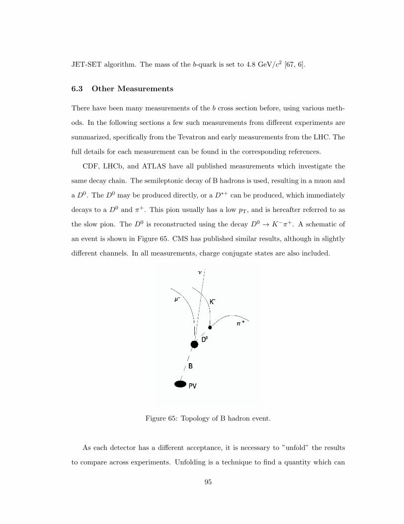
JET-SET algorithm. The mass of the b-quark is set to 4.8 GeV/c2 [67, 6].
6.3 Other Measurements
There have been many measurements of the b cross section before, using various meth-
ods. In the following sections a few such measurements from different experiments are
summarized, specifically from the Tevatron and early measurements from the LHC. The
full details for each measurement can be found in the corresponding references.
CDF, LHCb, and ATLAS have all published measurements which investigate the
same decay chain. The semileptonic decay of B hadrons is used, resulting in a muon and
a D0. The D0 may be produced directly, or a D∗+ can be produced, which immediately
decays to a D0 and π+. This pion usually has a low pT, and is hereafter referred to as
the slow pion. The D0 is reconstructed using the decay D0 → K−π+. A schematic of
an event is shown in Figure 65. CMS has published similar results, although in slightly
different channels. In all measurements, charge conjugate states are also included.
Figure 65: Topology of B hadron event.
As each detector has a different acceptance, it is necessary to ”unfold” the results
to compare across experiments. Unfolding is a technique to find a quantity which can
95

not be directly measured, by measuring a similar quantity. Then by comparing the
two quantities in Monte Carlo simulations, a matrix can be found to transform the
measured quantity into the desired quantity. In the case of these measurements, the
desired quantity is the pT(Hb) distribution, where Hb is the b-hadron, but since the Hb
can not be fully reconstructed due to at least the missing neutrino, only the pT(µD0)
distribution can be measured.
6.3.1 CDF measurement of b hadron production cross section
The Collider Detector at Fermilab (CDF) collaboration at the Fermilab Tevatron made
a measurement of the b hadron (Hb) production cross section in pp collisions at√s =
1.96 TeV [12]. The measurement uses an integrated luminosity of 83 pb−1 of data taken
with the CDF II detector. The detector consists of a charged particle tracker inside a
1.4 T solenoid magnet, calorimeters, and muon detectors.
In the reconstruction of an event, the kaon and pion candidate tracks are required
to originate from a displaced vertex which is consistent with the decay of a D0. To
include the decay D∗ → D0π, D0 → Kπ, the track of the slow pion is also required.
The branching ratios used in the measurement are B(Hb → µ−D0X)×B(D0 → K−π+)
for the µ−D0 mode and B(Hb → µ−D∗+X) × B(D∗+ → D0π+) × B(D0 → K−π+) for
the µ−D∗+ mode. The b hadron cross section is obtained by unfolding the measured
pT(µD0) distribution back to the pT(Hb) distribution. The differential cross section
is shown in Figure 66. The measured total cross section for b hadrons with pT >
9 GeV/c and |η| < 0.6 is shown in Equation 9, where 0.07(B) is the uncertainty from
the branching ratio.
σ(pp → HbX) = 1.30± 0.05(stat)± 0.14(syst)± 0.07(B) µb (9)
96
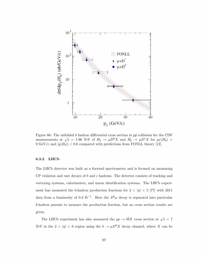
Figure 66: The unfolded b hadron differential cross section in pp collisions for the CDFmeasurements at
√s = 1.96 TeV of Hb → µD0X and Hb → µD∗X for pT (Hb) >
9 GeV/c and |y(Hb)| < 0.6 compared with predictions from FONLL theory [12].
6.3.2 LHCb
The LHCb detector was built as a forward spectrometer and is focused on measuring
CP violation and rare decays of b and c hadrons. The detector consists of tracking and
vertexing systems, calorimeters, and muon identification systems. The LHCb experi-
ment has measured the b-hadron production fractions for 2 < |η| < 5 [77] with 2011
data from a luminosity of 0.3 fb−1. Here the D0µ decay is separated into particular
b-hadron parents to measure the production fraction, but no cross section results are
given.
The LHCb experiment has also measured the pp → bbX cross section at√s = 7
TeV in the 2 < |η| < 6 region using the b → µD0X decay channel, where X can be
97

anything [13]. The measurement uses a branching ratio of B(b → D0Xµ−ν)× B(D0 →
K−π+), where B(b → D0Xµ−ν) = (6.84 ± 0.35)% and B(D0 → K−π+) = (3.89 ±
0.05)%. The collaboration used two independent data sets, collected at different times.
The first is from the earliest period of data taking, when the rate was low enough to
accept all events with at least one reconstructed track. This sample is called “microbias”
and has an integrated luminosity L = 2.9 nb−1. The second sample, called “triggered,”
was collected using a trigger which selects events with at least one muon. The triggered
sample has an integrated luminosity L = 12.2 nb−1. The two samples are analyzed
separately and then the results are combined.
To select signal events the D0 is reconstructed by combining a kaon and pion can-
didate whose tracks are inconsistent with originating at the primary vertex, and are
consistent with coming from a common decay vertex. The D0 candidate is matched
with a muon track to select an event likely belonging to the decay chain of interest.
The cross section as a function of η(µD0) is shown in Figure 67. The comparison with
two theoretical calculations is also shown. Averaging the data from both the microbias
and triggered data sets and summing over η(µD0) in the range 2 < η(µD0) < 6, the
measured cross section is shown in Equation 10. The results are consistent with the the-
oretical calculations within the theoretical uncertainties for both FONLL and MCFM
(not shown in the plot) [13].
σ(pp → bbX) = (75.3± 5.4± 13.0) µb (10)
6.3.3 ATLAS
The ATLAS experiment at the LHC has also published a measurement of the pp → bbX
cross section at√s = 7 TeV [14]. The ATLAS detector is a general purpose high
energy physics collider detector, similar to CMS, with tracking and vertexing detectors,
calorimeters, and muon identification systems covering almost the full solid angle around
98

Figure 67: LHCb measurement of σ(pp → HbX) as a function of η(µD0) [13] for themicrobias (×) and triggered (•) samples, shown displaced from the bin center and theaverage (+). In both data sets, pT (K,π) > 300 MeV is required. The muon pT isrequired to be at least 500 MeV for the microbias dataset and at least 1.3 GeV for thetriggered dataset. The data are shown as points with error bars, the MCFM predictionas a dashed line, and the FONLL prediction as a thick solid line. The thin upperand lower lines indicate the theoretical uncertainties on the FONLL prediction. Thesystematic uncertainties in the data are not included.
the collision point.
The data were taken during 2010 using a single muon trigger with pT > 6 GeV. The
total integrated luminosity of the data is 3.3 pb−1. The measurement uses the decay
b → D∗+µ−X,D∗+ → D0π+, D0 → K−π+. To reconstruct the events, all pairs of
opposite charge tracks are fit together to reconstruct the D0 , assigning each track the
kaon or pion mass. The D0 is then extrapolated back and fit with another track with
charge opposite to the one of the candidate kaon, which is assigned the pion mass, to
reconstruct the D∗. The D∗ candidate is fit with a muon to form the b-hadron vertex.
The number of candidates is found by fitting the distribution of the difference between
the mass of the D∗ candidate and the D0 candidate with a modified Gaussian.
The result is unfolded to get the differential cross section as a function of the pT and
|η| of the b-hadron, shown in Figure 68. An acceptance correction is applied to obtain
the integrated b-hadron cross section for pT (Hb) > 9 GeV and |η(Hb)| < 2.5, shown in
99

Equation 11. Here α denotes the uncertainty due to the acceptance correction, B is the
uncertainty due to the branching ratio, and L is the uncertainty due to the luminosity
measurement.
σ(pp → bbX) = 32.7± 0.8(stat.)± 3.1(syst.)+2.1−5.6(α)± 2.3(B)± 1.1(L) µb (11)
Figure 68: ATLAS measurement of σ(pp → HbX) unfolded and as a function of pT (Hb)(left) and |η(Hb)| (right) for pT (Hb) > 9 GeV/c and |η(Hb)| < 2.5, compared withtheoretical predictions. The inner error bars are the statistical uncertainties, and theouter error bars are the statistical plus total systematic uncertainties [14].
6.3.4 CMS
There have been previous measurements of the bb cross section with the CMS detector.
A measurement of the b-fraction for√s = 7 TeV of a sample of muon events exploiting
the transverse momentum of the muon with respect to the jet axis (prelT ) [6, 78] for
pT (µ) > 6 GeV/c and |η(µ)| < 2.1 showed that this inclusive cross section fell below the
predictions of PYTHIA [67], especially for the lower pT (µ) region, but above those for
MCNLO [69, 70], shown in Figure 69. The error in this analysis was dominated by the
systematic error which included a large contribution from the prelT template uncertainty.
A measurement of the correlated bb cross section measured with di-muons [79] also found
100
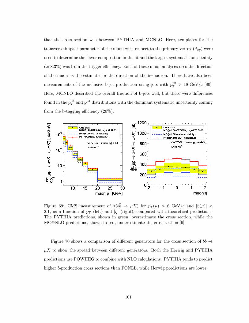
that the cross section was between PYTHIA and MCNLO. Here, templates for the
transverse impact parameter of the muon with respect to the primary vertex (dxy) were
used to determine the flavor composition in the fit and the largest systematic uncertainty
(- 8.3%) was from the trigger efficiency. Each of these muon analyses uses the direction
of the muon as the estimate for the direction of the b−hadron. There have also been
measurements of the inclusive b-jet production using jets with pjetT > 18 GeV/c [80].
Here, MCNLO described the overall fraction of b-jets well, but there were differences
found in the pjetT and yjet distributions with the dominant systematic uncertainty coming
from the b-tagging efficiency (20%).
Figure 69: CMS measurement of σ(bb → µX) for pT (µ) > 6 GeV/c and |η(µ)| <2.1, as a function of pT (left) and |η| (right), compared with theoretical predictions.The PYTHIA predictions, shown in green, overestimate the cross section, while theMC@NLO predictions, shown in red, underestimate the cross section [6].
Figure 70 shows a comparison of different generators for the cross section of bb →
µX to show the spread between different generators. Both the Herwig and PYTHIA
predictions use POWHEG to combine with NLO calculations. PYTHIA tends to predict
higher b-production cross sections than FONLL, while Herwig predictions are lower.
101
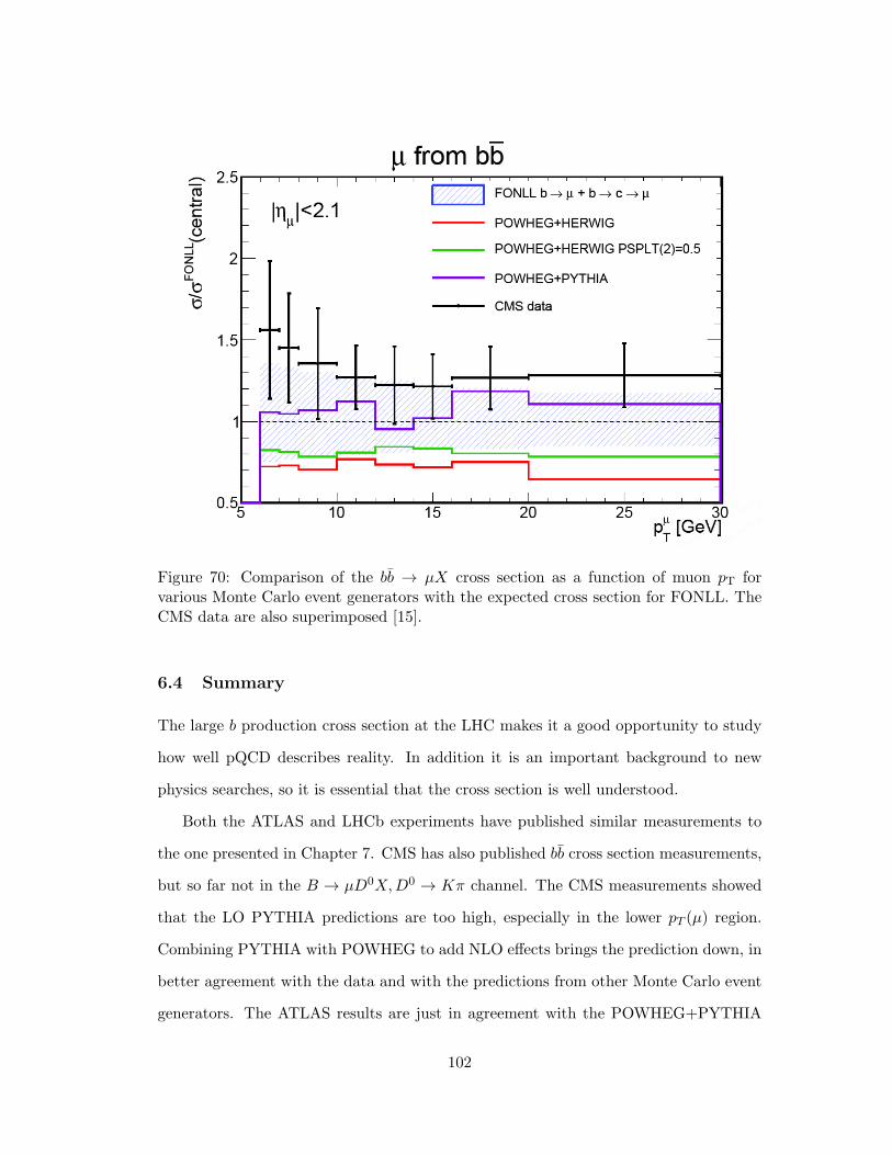
Figure 70: Comparison of the bb → µX cross section as a function of muon pT forvarious Monte Carlo event generators with the expected cross section for FONLL. TheCMS data are also superimposed [15].
6.4 Summary
The large b production cross section at the LHC makes it a good opportunity to study
how well pQCD describes reality. In addition it is an important background to new
physics searches, so it is essential that the cross section is well understood.
Both the ATLAS and LHCb experiments have published similar measurements to
the one presented in Chapter 7. CMS has also published bb cross section measurements,
but so far not in the B → µD0X,D0 → Kπ channel. The CMS measurements showed
that the LO PYTHIA predictions are too high, especially in the lower pT (µ) region.
Combining PYTHIA with POWHEG to add NLO effects brings the prediction down, in
better agreement with the data and with the predictions from other Monte Carlo event
generators. The ATLAS results are just in agreement with the POWHEG+PYTHIA
102
predictions within the errors. The LHCb results are consistent with FONLL predictions.
To compare results between experiments, the cross sections must be unfolded to
account for differences in acceptance. It is however difficult to compare between LHCb
and the two general-purpose experiments, because the overlapping region in η is small,
and ATLAS and CMS suffer from low efficiencies. The goals of this analysis are to
provide a cross section measurement at the LHC at relatively low muon pT , to provide
a complimentary measurement to the LHCb measurement for η < 2, and to provide a
potential direct comparison between CMS and LHCb.
103
7 bb Cross Section Measurement
7.1 Introduction
This chapter presents a measurement of the bb cross section at√s = 7 TeV using the
decay channel b → µ−D0X. Charge conjugate states are included. The differential cross
section is measured for pµD0
T > 6 GeV/c and |ηµD0 | < 2.4. Cross section measurements
from this decay channel provide a complimentary measurement to both the inclusive
muon and b-jet results. The direction of the b-hadron is better measured with the
addition of a D0 compared to those using only the muon direction, although we present
the differential cross section as a function of pT (D0µ) and η(D0µ) and not the b-hadron
direction. The low pT region helps to constrain predictions at small-x compared to the
CMS inclusive b-jet production results. Results from |η| > 2 are presented in order to
compare to those measured by LHCb.
The data were recorded with the CMS experiment at the Large Hadron Collider
(CERN) in 2010 using unprescaled single muon triggers corresponding to a total lumi-
nosity of 24 pb−1. One goal of this analysis is to provide information on the differential
cross section for low pT values (> 6 GeV/c) and η values greater than 2.1.
7.2 Data and Monte Carlo Samples
The data used in this analysis were obtained during the 2010 data taking period using
two single muon triggers, HLT Mu5 (pT (µ) > 5 GeV/c) and HLT Mu15 v1 (pT (µ) > 15
GeV/c). The single muon trigger HLT Mu5 (pT > 5 GeV/c) was prescaled early into
the 2010 data taking, so in addition the HLT Mu15 (pT > 15 GeV/c) trigger is used to
obtain more statistics for the higher pT b-hadron region. Only runs where the trigger was
unprescaled were used. The valid runs were specified using a JSON (JavaScript Object
Notation) file, which is a standard file format used to represent data structures in a
human-readable form. A run is considered good and valid for analysis when all detector
components are working fine and correctly calibrated and used in the reconstruction.
104
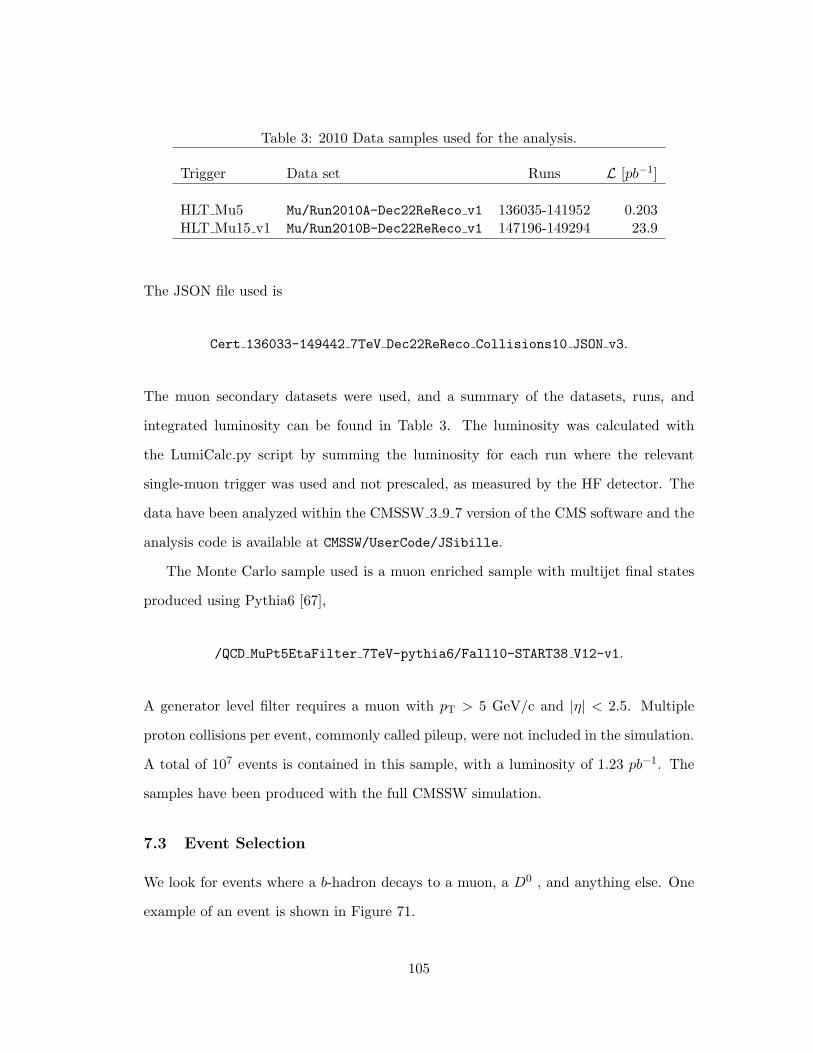
Table 3: 2010 Data samples used for the analysis.
Trigger Data set Runs L [pb−1]
HLT Mu5 Mu/Run2010A-Dec22ReReco v1 136035-141952 0.203HLT Mu15 v1 Mu/Run2010B-Dec22ReReco v1 147196-149294 23.9
The JSON file used is
Cert 136033-149442 7TeV Dec22ReReco Collisions10 JSON v3.
The muon secondary datasets were used, and a summary of the datasets, runs, and
integrated luminosity can be found in Table 3. The luminosity was calculated with
the LumiCalc.py script by summing the luminosity for each run where the relevant
single-muon trigger was used and not prescaled, as measured by the HF detector. The
data have been analyzed within the CMSSW 3 9 7 version of the CMS software and the
analysis code is available at CMSSW/UserCode/JSibille.
The Monte Carlo sample used is a muon enriched sample with multijet final states
produced using Pythia6 [67],
/QCD MuPt5EtaFilter 7TeV-pythia6/Fall10-START38 V12-v1.
A generator level filter requires a muon with pT > 5 GeV/c and |η| < 2.5. Multiple
proton collisions per event, commonly called pileup, were not included in the simulation.
A total of 107 events is contained in this sample, with a luminosity of 1.23 pb−1. The
samples have been produced with the full CMSSW simulation.
7.3 Event Selection
We look for events where a b-hadron decays to a muon, a D0 , and anything else. One
example of an event is shown in Figure 71.
105
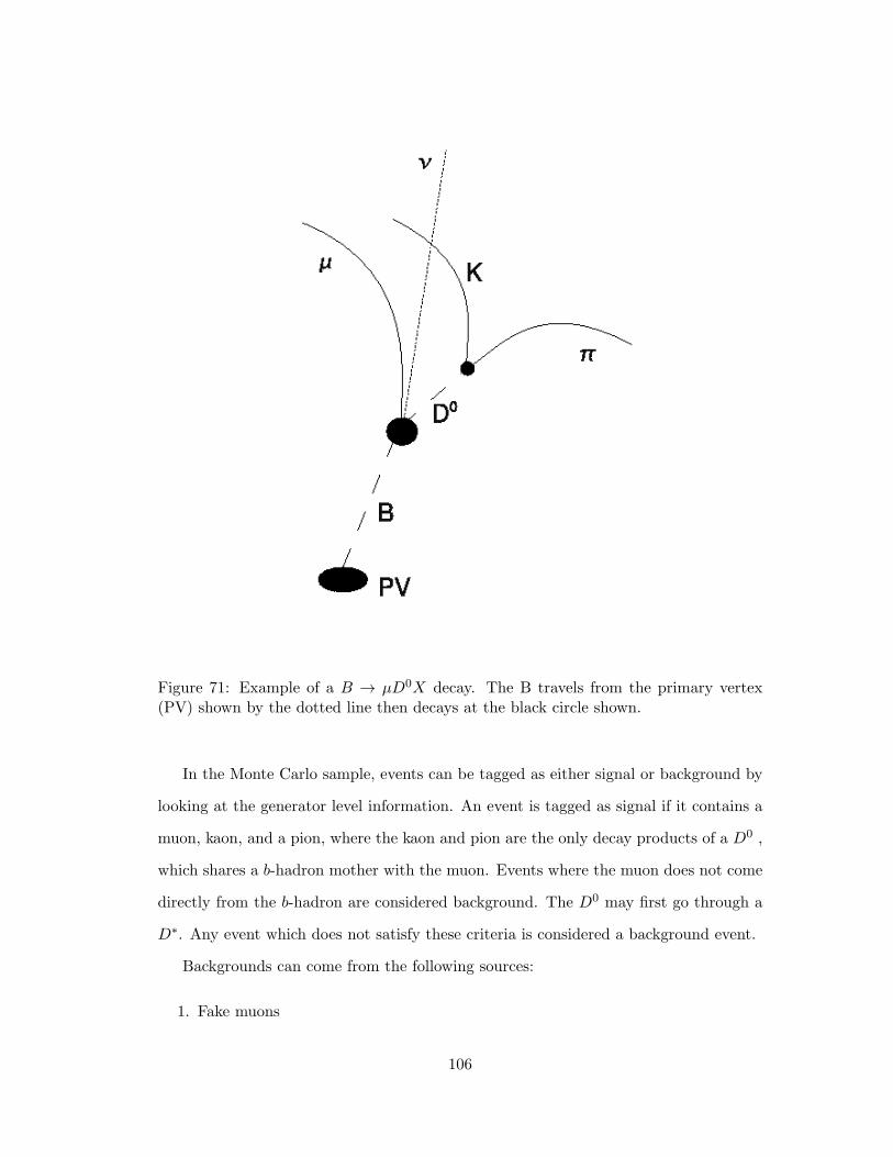
Figure 71: Example of a B → µD0X decay. The B travels from the primary vertex(PV) shown by the dotted line then decays at the black circle shown.
In the Monte Carlo sample, events can be tagged as either signal or background by
looking at the generator level information. An event is tagged as signal if it contains a
muon, kaon, and a pion, where the kaon and pion are the only decay products of a D0 ,
which shares a b-hadron mother with the muon. Events where the muon does not come
directly from the b-hadron are considered background. The D0 may first go through a
D∗. Any event which does not satisfy these criteria is considered a background event.
Backgrounds can come from the following sources:
1. Fake muons
106
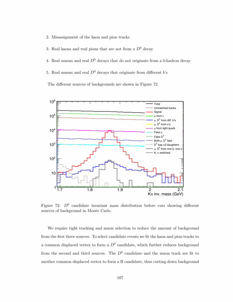
2. Misassignment of the kaon and pion tracks
3. Real kaons and real pions that are not from a D0 decay
4. Real muons and real D0 decays that do not originate from a b-hadron decay
5. Real muons and real D0 decays that originate from different b’s
The different sources of backgrounds are shown in Figure 72.
inv. mass (GeV)πK1.7 1.8 1.9 2 2.11
10
210
310
410
510
610 TotalUnmatched tracksSignal
τ from µ
from diff. b’s0, Dµ
from c’s0, Dµ
from light quarkµ
µFake 0Fake D
fake0, DµBoth has >2 daughters0D
from one b, one c0, Dµ
switchedπK,
Figure 72: D0 candidate invariant mass distribution before cuts showing differentsources of background in Monte Carlo.
We require tight tracking and muon selection to reduce the amount of background
from the first three sources. To select candidate events we fit the kaon and pion tracks to
a common displaced vertex to form a D0 candidate, which further reduces background
from the second and third sources. The D0 candidate and the muon track are fit to
another common displaced vertex to form a B candidate, thus cutting down background
107

from the fourth source. The KinematicParticleVertexFitter [81] is used to create a
kinematic particle from the daughter particles. A skim is run to extract interesting
events before the full analysis (selection) cuts are applied to enhance the b-hadron
signature sensitivity. We separate the events into the correct sign combinations (whhere
the muons and kaons have the same charge) and wrong sign combinations. After the
selection cuts with the correct charge assignments, we find only D0 candidates from the
signal should be present as a resonance in the invariant K−π+ mass spectrum (charge
conjugate states are included), which is fit to extract the signal.
7.3.1 Acceptance and Quality Cuts
A first set of cuts is made in order to assure the quality of the selected events. Events
with no more than 1000 tracks are chosen. For the muon, kaon, and pion tracks
we require hits in at least 2 pixel layers to ensure that only good quality tracks are
used. Additionally, we require at least 10 tracker hits (pixels plus strips) for the muon
track, and at least 5 tracker hits for the kaon and the pion tracks. Muons satisfy the
GlobalMuonPromptTight criteria [82]. The muon, kaon, and pion tracks must have
|η| < 2.4. The muon is required to have pT > 5 GeV/c, while the kaon and pion are
required to have pT > 0.5 GeV/c. Figure 73 shows the pT and η distributions for
the muon candidates in Monte Carlo events and the 2010A data, while Figure 74 shows
these distributions for the kaon/pion track candidates. The kaon candidate and the pion
candidate must have opposite charges, but there are no explicit particle identification
cuts placed on either of them.
Cuts of ∆R(µK) ≤ 1.5 and ∆R(µπ) ≤ 1.5 are made to increase the probability
that the muon, kaon, and pion come from a b-hadron. Here, ∆R =√
∆φ2 +∆η2.
The distributions for ∆R are shown for signal and background Monte Carlo events in
Figure 75. The kaon candidate track and the pion candidate track form a D0 candidate
which is required to have an invariant mass (using the particle data group (PDG)
masses for each of the kaon and pion) within 0.3 GeV/c2 of the mass of the D0 (1.8646
108

) (GeV/c)µ(T
p0 5 10 15 200
0.05
0.1
0.15
0.2
610×
Data
Monte Carlo
)µ(η-2 0 20
20
40
60
80
310×
Data
Monte Carlo
Figure 73: Distributions of pT (left) and η (right) for tracks identified as tight muonsshown after the track quality cuts for Monte Carlo events (filled histogram) and 2010Adata events (points). The Monte Carlo is normalized to the Run A luminosity.
) (GeV/c)π(K,T
p0 2 4 6 8 100
0.1
0.2
0.3
0.4
610×
Data
Monte Carlo
)π(K,η-2 0 20
20
40
60
310×
Data
Monte Carlo
Figure 74: Distributions of pT (left) and η (right) for kaon/pion tracks shown afterthe track quality cuts for Monte Carlo events (filled histogram) and 2010A data events(points). The Monte Carlo is normalized to the run A luminosity.
GeV/c2) [83]. This “D0 ” mass distribution after the skim cuts for both the 2010A and
2010B datasets is shown in Figure 76, and for Monte Carlo events in Figure 77. We also
require that the vertex probability for both the D0 and B candidates is greater than
0.01, to eliminate cases where the vertex fit fails.
The masses of the B± and B0 mesons are 5.28 GeV/c2 [83], so we require that the
invariant mass of the µD0 candidate is less than 5 GeV/c2. Since we do not reconstruct
any other possible daughters of the B meson there is no minimum requirement on
the µD0 invariant mass. The µD0 candidate invariant mass distribution is shown in
109

Figure 75: Distributions of ∆R(µ,K) (left) and ∆R(µ,π) (right) after skim cuts fortagged signal (red) and background (black) Monte Carlo events. The distributions arenormalized to unit area.
)2 inv. mass (GeV/cπK1.7 1.8 1.9 2 2.1
50
60
70
80
310×
)2 inv. mass (GeV/cπK1.7 1.8 1.9 2 2.1
0.1
0.15
0.2
610×
Figure 76: The K−π+ invariant mass distribution for the 2010A dataset (left) and2010B dataset (right) after the acceptance and quality cuts.
Figure 78 for signal and background Monte Carlo events.
In summary, the following cuts are made for acceptance and track quality.
1. The primary vertex must have a longitudinal impact parameter less than 24 cm.
2. All tracks must have |η| < 2.4.
3. The muon and kaon are required to have ∆R(µ,K) ≤ 1.5.
4. The muon and pion are required to have ∆R(µ,π) ≤ 1.5.
5. The muon track must have pT > 5 GeV/c.
110

)2 inv. mass (GeV/cπK1.7 1.8 1.9 2 2.10
0.05
0.1
0.15
0.2
0.25Signal
Background
Figure 77: The K−π+ invariant mass distribution for tagged signal (red) and back-ground (black) Monte Carlo events after the acceptance and quality cuts. The distri-butions are normalized to unit area.
2 4 6 8 100
20
40
60
-310×
hbcTruthBMassEntries 49120Mean 3.859RMS 0.5218
µD0 inv. mass (GeV/c2)
Figure 78: The µD0 invariant mass distribution for tagged signal (red) and background(black) Monte Carlo events after the acceptance cuts. The distributions are normalizedto unit area.
6. The kaon and pion candidate tracks are required to have pT > 0.5 GeV/c.
7. The mass of the D0µ must be less than 5 GeV/c2.
8. The D0 vertex probability must be greater than 0.01.
9. The B vertex probability must be greater than 0.01.
Table 4 shows the cuts which are made for acceptance and track quality cuts. There
are 49K signal candidates and 515M background candidates in the Monte Carlo before
the acceptance cuts.
111

Table 4: Variables used for acceptance and quality cuts and their cut values. TheSignal Eff and BG MC Eff columns show the efficiencies of the truth matched signaland background events, respectively, after each cut.
Variable Cut Value Signal Eff BG MC EffPV long. IP < 24 cm 1 - 1Track quality see text 0.88 0.65pT (µ) ≥ 5 GeV/c 1 1|η(µ)| < 2.4 1 1pT (K,π) ≥ 0.7 GeV/c 0.83 0.32|η(K,π)| < 2.4 0.97 0.97∆R(µK, µπ) < 1.5 0.98 0.46µD0 mass < 5 GeV/c2 0.99 0.29Vertex prob. > 0.01ALL quality cuts 0.70 0.04
7.3.2 Selection Cut Variables
In order to avoid the trigger turn-on region, the cut on the muon pT is raised 1 GeV/c
above the trigger pT value (6 GeV/c for the HLT Mu5-triggered data, and 16 GeV/c
for the HLT Mu15 v1-triggered data). Additional cuts are added at the analysis level
including event cuts, D0 candidate cuts, and b-hadron candidate cuts. We consider
using the following variables, which are described in the following sections, for the event
selection after the quality cuts have been made:
1. D0 doca
2. B doca
3. D0 3D flight distance
4. B 3D flight distance
5. muon signed transverse impact parameter
6. xb
7. D0 pointing angle
112

8. B pointing angle
D0 and B doca From the KinematicVertexParticleFitter, the distance of closest ap-
proach (doca) for each of the D0 and b-hadron candidates can be found. The doca is
defined to be the distance between two tracks at their point of closest approach. Fig-
ure 79 shows how the doca is defined for the D0 vertex. Figure 80 shows the signal and
data distributions of the doca for the D0 and b-hadron candidates.
Figure 79: Definition of the distance of closest approach (doca).
D0 and B 3D Flight Distance Significance The 3D flight distance significance
can also be found for each of the D0 and b-hadron candidates from the KinematicVert-
exParticleFitter. Figure 81 shows the distribution of the 3D flight distance for the D0
and b-hadron candidates.
Muon Signed Transverse Impact Parameter The muon signed transverse impact
parameter can be determined as the distance of closest approach of the muon track to
the primary vertex, with the sign determined by the angle between a line connecting
113

doca (cm)0D0 10 20 30 40 50
-310×0
20
40
60
80
-310×
Signal
Background
B doca (cm)0 5 10 15 20 25 30
-310×0
0.05
0.1
0.15
Signal
Background
Figure 80: Distributions of the D0 (left) and b-hadron (right) candidate doca (right)after all other selection cuts for tagged signal (red) and background (black) Monte Carloevents. The distributions are normalized to unit area.
the primary vertex with the point of closest approach and a reference direction, which
is the direction of the D0 candidate. This is shown in Figure 82. The signed muon
transverse impact distributions found for signal and data are shown in Figure 83. As
one can see, the distribution is symmetric for the background case, and is asymmetric
in the case of the signal. This indicates that the muon came from a long-lived particle,
which is more likely to have a positive signed impact parameter.
xb Variable We make a requirement on the isolation of the µD0 candidate using the
variable xb, which is the pT of the b-hadron candidate divided by the sum of the pT
of all other tracks (with pT > 0.5 GeV/c) within a cone of ∆R less than 1 around the
b-hadron candidate. Mathematically this is defined as
xb =pT(µD0)
∑
∆R(µD0,X)<1 pT(X)(12)
Signal candidates will tend to have larger values in this variable as can be seen by the
distributions shown in Figure 84.
Since the xb variable is a measure of the isolation of the B candidate, it depends
on the fragmentation and on the underlying event. In addition, since the B is not fully
reconstructed, this variable is blurred. The distributions of the xb variable in data and
114
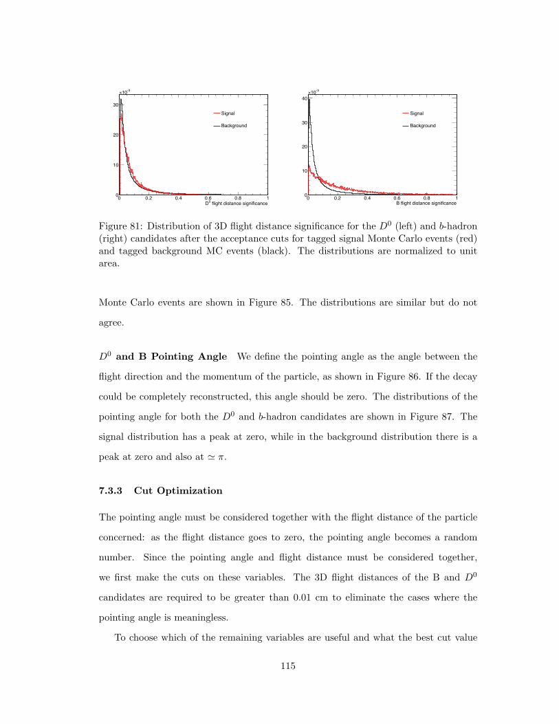
flight distance significance0D0 0.2 0.4 0.6 0.8 10
10
20
30
-310×
Signal
Background
B flight distance significance0 0.2 0.4 0.6 0.8 10
10
20
30
40-310×
Signal
Background
Figure 81: Distribution of 3D flight distance significance for the D0 (left) and b-hadron(right) candidates after the acceptance cuts for tagged signal Monte Carlo events (red)and tagged background MC events (black). The distributions are normalized to unitarea.
Monte Carlo events are shown in Figure 85. The distributions are similar but do not
agree.
D0 and B Pointing Angle We define the pointing angle as the angle between the
flight direction and the momentum of the particle, as shown in Figure 86. If the decay
could be completely reconstructed, this angle should be zero. The distributions of the
pointing angle for both the D0 and b-hadron candidates are shown in Figure 87. The
signal distribution has a peak at zero, while in the background distribution there is a
peak at zero and also at - π.
7.3.3 Cut Optimization
The pointing angle must be considered together with the flight distance of the particle
concerned: as the flight distance goes to zero, the pointing angle becomes a random
number. Since the pointing angle and flight distance must be considered together,
we first make the cuts on these variables. The 3D flight distances of the B and D0
candidates are required to be greater than 0.01 cm to eliminate the cases where the
pointing angle is meaningless.
To choose which of the remaining variables are useful and what the best cut value
115

Figure 82: Definition of the muon signed transverse impact parameter.
is we optimize the significance of each variable. The significance is defined as S/√B,
where S is the number of tagged signal Monte Carlo events passing the cut, and B is
the number of background Monte Carlo events passing the cut. The direction of the
cut is based on looking at the distributions of the signal and background Monte Carlo
events for each variable, and choosing it such that more signal than background events
pass the cut. Specifically, for the µ signed transverse impact parameter, D0 and B
flight distance significance, and xb, the event is defined as passing the cut if the value
is greater than the cut value. For the D0 and B doca and pointing angle, the event is
defined as passing the cut if the value is less than the cut value.
A subset of the Monte Carlo events is used for the cut tuning. We start with a subset
of 1M candidates after the quality cuts, with 1439 of those being true signal. After the
cuts on the distance and pointing angle variables, there were 324028 total candidates
(1105 signal candidates and 322923 background candidates).
116

transverse impact parameter (cm)µ-1 -0.5 0 0.5 1
-710
-610
-510
-410
-310
-210
-110Signal
Background
Figure 83: Distribution of muon signed impact parameter shown after the acceptancecuts for tagged signal Monte Carlo events (red) and tagged background MC events(black). The distributions are normalized to unit area.
bx0 0.2 0.4 0.6 0.8 10
5
10
15
20
25
-310×
Signal
Background
Figure 84: Distributions of xb after all acceptance cuts for tagged signal Monte Carloevents (red) and background MC events (black). The distributions are normalized tounit area.
We use a sequential procedure to tune the cuts. For the first pass, we look at the
significance distribution for each of the variables under consideration. We choose the
variable with the highest significance as the first variable to use as a selection cut.
The value is determined by finding the maximum of the significance distribution. The
distributions for the first pass are shown in Figure 88.
From these distributions we determine that the xb variable has the best significance
after the acceptance cuts, and the significance is maximum at a cut value of 0.7. For
the second pass, we require xb > 0.7 and repeat the procedure for all other variables.
117

bx0 0.2 0.4 0.6 0.8 10
5
10
15
20
25
-310×
Run ARun BMonte CarloMonte Carlo
)>15GeVµ(T
p
Figure 85: Distributions of xb for Monte Carlo events (red), Monte Carlo events withpT(µ) > 15 GeV/c (purple), Run A data events (black), and Run B data events (blue).The distributions are normalized to unit area.
The distributions for the second pass are shown in Figure 89.
After the second pass we determine that the B doca shows the best significance. The
maximum is at a cut value of 0.007. For the third pass, we repeat the procedure, re-
quiring that both xb > 0.7 and the B doca < 0.007. The distributions for the remaining
variables after the third pass are shown in Figure 90.
The D0 doca shows the best discrimination between signal and background after
the third pass. The significance is at its maximum at a cut value of 0.015. For the
fourth pass, we require xb > 0.7, the B doca < 0.007, and the D0 doca < 0.015. The
distribution for the muon transverse impact parameter after the fourth is shown in
Figure 91.
The muon transverse impact parameter does not give any significant discrimination
between signal and background except in the right tail of the distribution. This would
severely reduce the statistics, and so it does not make sense to use a cut on this variable.
Finally, for the event selection we require:
1. xb greater than 0.7
2. B doca less than 0.007
3. D0 doca less than 0.015
118
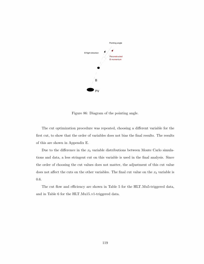
PV
B
B flight direction
Reconstructed
B momentum
Pointing angle
Figure 86: Diagram of the pointing angle.
The cut optimization procedure was repeated, choosing a different variable for the
first cut, to show that the order of variables does not bias the final results. The results
of this are shown in Appendix E.
Due to the difference in the xb variable distributions between Monte Carlo simula-
tions and data, a less stringent cut on this variable is used in the final analysis. Since
the order of choosing the cut values does not matter, the adjustment of this cut value
does not affect the cuts on the other variables. The final cut value on the xb variable is
0.6.
The cut flow and efficiency are shown in Table 5 for the HLT Mu5-triggered data,
and in Table 6 for the HLT Mu15 v1-triggered data.
119
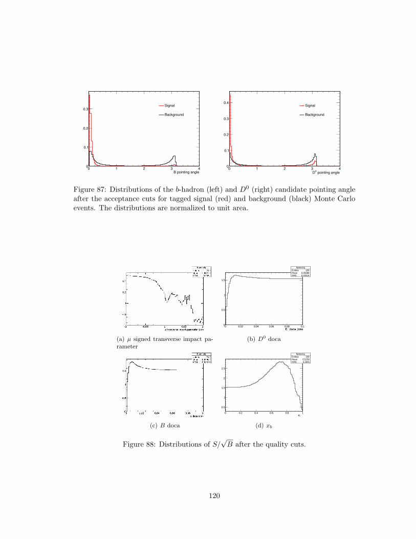
B pointing angle0 1 2 3 40
0.1
0.2
0.3Signal
Background
pointing angle0D0 1 2 3 40
0.1
0.2
0.3
0.4Signal
Background
Figure 87: Distributions of the b-hadron (left) and D0 (right) candidate pointing angleafter the acceptance cuts for tagged signal (red) and background (black) Monte Carloevents. The distributions are normalized to unit area.
(a) µ signed transverse impact pa-rameter
hpasssigEntries 100Mean 0.05088RMS 0.02814
0 0.02 0.04 0.06 0.08 0.10
0.5
1
1.5
hpasssigEntries 100Mean 0.05088RMS 0.02814
(b) D0 doca
(c) B doca
hpasssigEntries 100Mean 0.5239RMS 0.2641
0 0.2 0.4 0.6 0.8 1
0.5
1
1.5
2
2.5
hpasssigEntries 100Mean 0.5239RMS 0.2641
(d) xb
Figure 88: Distributions of S/√B after the quality cuts.
120
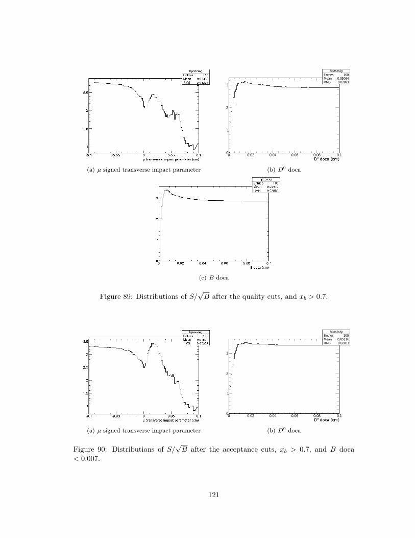
(a) µ signed transverse impact parameter
hpasssigEntries 100Mean 0.05064RMS 0.02821
0 0.02 0.04 0.06 0.08 0.10
1
2
3
hpasssigEntries 100Mean 0.05064RMS 0.02821
(b) D0 doca
(c) B doca
Figure 89: Distributions of S/√B after the quality cuts, and xb > 0.7.
(a) µ signed transverse impact parameter
hpasssigEntries 100Mean 0.05116RMS 0.02811
0 0.02 0.04 0.06 0.08 0.10
1
2
3
hpasssigEntries 100Mean 0.05116RMS 0.02811
(b) D0 doca
Figure 90: Distributions of S/√B after the acceptance cuts, xb > 0.7, and B doca
< 0.007.
121
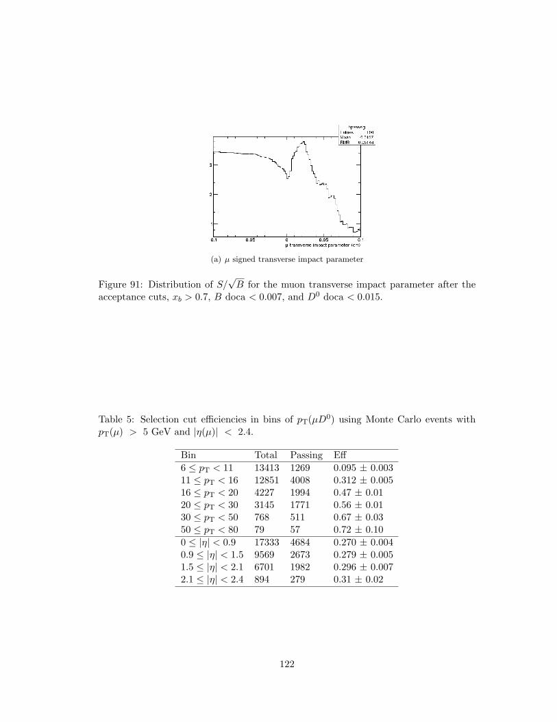
(a) µ signed transverse impact parameter
Figure 91: Distribution of S/√B for the muon transverse impact parameter after the
acceptance cuts, xb > 0.7, B doca < 0.007, and D0 doca < 0.015.
Table 5: Selection cut efficiencies in bins of pT(µD0) using Monte Carlo events withpT(µ) > 5 GeV and |η(µ)| < 2.4.
Bin Total Passing Eff6 ≤ pT < 11 13413 1269 0.095 ± 0.00311 ≤ pT < 16 12851 4008 0.312 ± 0.00516 ≤ pT < 20 4227 1994 0.47 ± 0.0120 ≤ pT < 30 3145 1771 0.56 ± 0.0130 ≤ pT < 50 768 511 0.67 ± 0.0350 ≤ pT < 80 79 57 0.72 ± 0.100 ≤ |η| < 0.9 17333 4684 0.270 ± 0.0040.9 ≤ |η| < 1.5 9569 2673 0.279 ± 0.0051.5 ≤ |η| < 2.1 6701 1982 0.296 ± 0.0072.1 ≤ |η| < 2.4 894 279 0.31 ± 0.02
122

Table 6: Selection cut efficiencies in bins of pT(µD0) using Monte Carlo events withpT(µ) > 15 GeV and |η(µ)| < 2.4.
Bin Total Passing Eff16 ≤ pT < 20 35 0 020 ≤ pT < 30 646 231 0.36 ± 0.0230 ≤ pT < 50 442 262 0.59 ± 0.0450 ≤ pT < 80 58 39 0.67 ± 0.110 ≤ |η| < 0.9 637 275 0.43 ± 0.030.9 ≤ |η| < 1.5 281 129 0.46 ± 0.041.5 ≤ |η| < 2.1 229 113 0.49 ± 0.052.1 ≤ |η| < 2.4 42 23 0.55 ± 0.11
123

7.4 Efficiencies
The efficiency can be broken into three parts: the tracking and reconstruction efficiency
(εrec), the trigger efficiency (εtrig), and the cut efficiency (εcut). The formula is given in
Equation 13. Each of these parts is described separately in the following sections. The
efficiency is calculated in bins of the pT and η of the µD0.
ε = εrec · εcut · εtrig (13)
The tracking and reconstruction efficiency and the cut efficiency can be found using
Monte Carlo. One method is to apply the full analysis procedure to the Monte Carlo
and fit the Kπ invariant mass distributions to find the number of µD0 candidates. The
fits are shown in Figures 92 and 93, and Figures 94 and 95 for bins of pT (µ) and |η(µ)|,
respectively.
The distributions are fit with a double Gaussian function plus a linear background,
shown in Equation 14. The Gaussians are required to have the same center, described
by parameter p2. Parameters p0 and p1 describe the linear background, parameters p3
and p4 describe the amplitudes of the Gaussians, and parameters p5 and p6 describe
the widths of the Gaussians. The fits are done using binned likelihood fits, in order to
sensibly model the background in low statistics bins. The minimization is done with
the MINUIT package [84] in ROOT [85]. For variables with a Gaussian distribution,
the likelihood is related to the χ2, as shown in Equation 15. The likelihood fits provide
a χ2 value which can be used as an approximate goodness-of-fit estimate.
y = p0 + p1 · x+ p3e−1
2
(
x−p2p5
)2
+ p4e−1
2
(
x−p2p6
)2
(14)
χ2 ∝ −2 lnL (15)
The number of D0 candidates can be calculated from the fit parameters according
124

to Equation 16, where p3 and p4 are the amplitudes of the double Gaussian, p5 and p6
are the standard deviations of the double Gaussian, and ∆m is the bin size of the Kπ
invariant mass distribution.
N(D0) =
√2π
∆m(p3p5 + p4p6) (16)
The efficiency is defined as the number of D0 candidates from the fit divided by the
number of signal events generated in the acceptance. The efficiency for the tracking,
reconstruction, and event selection is shown in Figures 96 and 97.
Due to the low statistics, the efficiencies have very large errors in some bins. This
contributes a large systematic uncertainty to the final result. Another method to find
the efficiencies is to use the tagged Monte Carlo. A potential problem with this method
would be if there was a significant fraction of signal events which are not in the mass
peak, or if there is a peak in the background in the peak region. In addition, the
tagging in Monte Carlo is not 100% efficient. Sometimes the reconstructed tracks can
not be matched to the generator level particles. In the event that these effects would
be significant, it would be necessary to use the fit method. These are not expected to
be significant effects, so the tagged Monte Carlo efficiencies are used in this analysis.
For more details, and plots of the different backgrounds at each step of the selection
procedure, separated into categories, see Appendix D.
The efficiency found from the tagged Monte Carlo compared with the efficiency found
from the Monte Carlo fits is shown in Figure 98 as a function of pT , and in Figure 99 as
a function of |η|. The efficiencies are completely consistent with each other. Therefore
the efficiencies from the tagged Monte Carlo are used, since they contribute much less
to the systematic uncertainty. The total reconstruction and selection efficiencies are
shown in Table 7.
125

Table 7: The reconstruction and selection efficiency (εrec · εcut) in each pT (µD0) and|η(µD0)| bin. The Eff5 column is using Monte Carlo events with pT (µ) > 5 GeV, andthe Eff15 column is using Monte Carlo events with pT (µ) > 15 GeV. In both cases|η(µ)| < 2.4 is required.
Bin Eff5 Eff156 ≤ pT < 11 0.042 ± 0.001 –11 ≤ pT < 16 0.21 ± 0.003 –16 ≤ pT < 20 0.35 ± 0.008 –20 ≤ pT < 30 0.43 ± 0.01 0.27 ± 0.0230 ≤ pT < 50 0.51 ± 0.02 0.47 ± 0.0350 ≤ pT < 80 0.48 ± 0.06 0.44 ± 0.070 ≤ |η| < 0.9 0.17 ± 0.002 0.33 ± 0.020.9 ≤ |η| < 1.5 0.16 ± 0.003 0.30 ± 0.031.5 ≤ |η| < 2.1 0.14 ± 0.003 0.32 ± 0.032.1 ≤ |η| < 2.4 0.07 ± 0.004 0.21 ± 0.04
7.4.1 Trigger Efficiency
The muon trigger which is used to select the data is not 100% efficient, so in order to
determine how many events were produced, the observed events must be corrected for
the trigger efficiency. Since it is a muon trigger, the trigger efficiency depends on the
pT and η of the muon. The Monte Carlo does not require a trigger to select the events,
so no correction for the trigger efficiency is required.
The trigger efficiencies are calculated using independently triggered data sets: an
electron-triggered data set for the HLT Mu5 trigger, and a jet-triggered data set for the
HLT Mu15 v1 trigger. The data sets used are listed in Table 8. The method is described
in detail in [86]. The efficiency is calculated by looking at muons which are reconstructed
offline, and then matching them to the HLT muons. The muons are matched to the
HLT muons by searching within a cone of ∆R < 0.5. The muons are required to satisfy
the GlobalMuonPromptTight criteria. In order to reduce the possibility of mismatching,
the events are required to have only one reconstructed muon.
In order to further reduce background from pion and kaon decays, as well as from
punch-through hadrons, the muons are chosen to come from semileptonic heavy flavor
126

Table 8: 2010 Data samples used for the trigger efficiency calculation.
Trigger Data set
HLT Mu5 EG/Run2010A-Nov4ReReco v1/AOD
HLT Mu15 v1 /Jet/Run2010B-Dec22ReReco v1/AOD
decays by selecting muons in b-tagged jets. The trigger efficiencies for muons in b-tagged
jets are generally lower than for isolated muons due to the density of tracks. As this
analysis uses muons coming from semileptonic b decays, this method is particularly
appropriate.
The efficiencies, in bins of pT (µ) and |η(µ)|, are shown in Figures 100 and 101 for
the HLT Mu5 trigger, and in Figures 102 and 103 for the HLT Mu15 v1 trigger.
Since we ultimately want to measure the cross section as a function of the pT and η
of the µD0 candidate, the trigger efficiency can not be simply multiplied with the other
efficiencies. In addition, the two data sets use different triggers, so we must correct
for the trigger efficiencies in order to compare results between the two data sets. We
therefore apply a weighting of 1εtrig
to the data in the Kπ invariant mass distribution
before fitting. The Monte Carlo does not need to be corrected for trigger efficiency. The
effect of the trigger efficiency weighting can be seen in Figure 104.
127

(GeV)πKm1.75 1.8 1.85 1.9 1.95 2
entri
es
0
100
200
300
400
hacD0MassRightQ_pt5Entries 4501Mean 1.862RMS 0.04335
/ ndf 2χ 29.83 / 21Prob 0.0955p0 26.8± 240.7 p1 14.0± -114.8 p2 0.000± 1.865 p3 26.1± 133 p4 13.4± 241.2 p5 0.0000± 0.0065 p6 0.000± 0.017
(a) 6 ≤ pT < 11
(GeV)πKm1.75 1.8 1.85 1.9 1.95 2
entri
es
0
0.2
0.4
0.6
0.8
1
1.2
310×
hacD0MassRightQ_pt10Entries 12287Mean 1.861RMS 0.04119
/ ndf 2χ 79.49 / 21Prob 9.812e-09p0 42.5± 727 p1 22.1± -352.1 p2 0.000± 1.865 p3 45.7± 504.7 p4 23.0± 735.3 p5 0.0000± 0.0065 p6 0.000± 0.017
(b) 11 ≤ pT < 16
(GeV)πKm1.75 1.8 1.85 1.9 1.95 2
entri
es
0
200
400
600
hacD0MassRightQ_pt15Entries 6368Mean 1.862RMS 0.04247
/ ndf 2χ 26.07 / 21Prob 0.2038p0 10.4± 331.6 p1 5.4± -157.2 p2 0.000± 1.865 p3 32.3± 258.8 p4 16.3± 364.2 p5 0.0000± 0.0065 p6 0.000± 0.017
(c) 16 ≤ pT < 20
(GeV)πKm1.75 1.8 1.85 1.9 1.95 2
entri
es
0
200
400
600
hacD0MassRightQ_pt20Entries 6049Mean 1.862RMS 0.04518
/ ndf 2χ 28.04 / 21Prob 0.1391p0 34.8± 399.2 p1 18.2± -190.9 p2 0.000± 1.865 p3 31.0± 229.5 p4 15.7± 323.5 p5 0.0000± 0.0065 p6 0.000± 0.017
(d) 20 ≤ pT < 30
(GeV)πKm1.75 1.8 1.85 1.9 1.95 2
entri
es
0
50
100
150
hacD0MassRightQ_pt30Entries 1749Mean 1.863RMS 0.04583
/ ndf 2χ 8.971 / 21Prob 0.9894p0 19.52± 87.05 p1 10.25± -39.52 p2 0.000± 1.865 p3 16.94± 62.42 p4 8.9± 99.2 p5 0.0000± 0.0065 p6 0.000± 0.017
(e) 30 ≤ pT < 50
Figure 92: D0 mass distributions in bins of pT (µD0 ) (GeV/c) for Monte Carlo eventswith |η(µ,K,π)| < 2.4, pT(µ) > 6 GeV/c, and pT(K,π) > 0.5 GeV/c. The distributionsare fit with a linear background plus a double Gaussian signal.
128
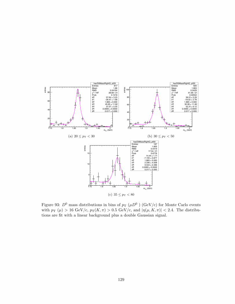
(GeV)πKm1.75 1.8 1.85 1.9 1.95 2
entri
es
0
20
40
60
80
hacD0MassRightQ_pt20Entries 817Mean 1.86RMS 0.04164
/ ndf 2χ 28.69 / 21Prob 0.1216p0 3.23± 57.64 p1 1.68± -28.47 p2 0.000± 1.865 p3 11.82± 45.65 p4 5.55± 37.07 p5 0.0000± 0.0065 p6 0.000± 0.017
(a) 20 ≤ pT < 30
(GeV)πKm1.75 1.8 1.85 1.9 1.95 2
entri
es0
20
40
60
80
100
hacD0MassRightQ_pt30Entries 925Mean 1.863RMS 0.0429
/ ndf 2χ 41.06 / 21Prob 0.00552p0 5.29± 39.51 p1 2.78± -18.02 p2 0.000± 1.865 p3 11.60± 30.08 p4 6.12± 52.31 p5 0.0000± 0.0065 p6 0.000± 0.017
(b) 30 ≤ pT < 50
(GeV)πKm1.75 1.8 1.85 1.9 1.95 2
entri
es
0
5
10
15
hacD0MassRightQ_pt50Entries 167Mean 1.855RMS 0.0419
/ ndf 2χ 17.54 / 21Prob 0.6776p0 1.71± 14.44 p1 0.877± -7.155 p2 0.000± 1.865 p3 4.508± 2.336 p4 2.496± 9.544 p5 0.0000± 0.0065 p6 0.000± 0.017
(c) 35 ≤ pT < 80
Figure 93: D0 mass distributions in bins of pT (µD0 ) (GeV/c) for Monte Carlo eventswith pT (µ) > 16 GeV/c, pT(K,π) > 0.5 GeV/c, and |η(µ,K,π)| < 2.4. The distribu-tions are fit with a linear background plus a double Gaussian signal.
129

(GeV)πKm1.75 1.8 1.85 1.9 1.95 2
entri
es
0
0.5
1
1.5
2310×
hacD0MassRightQ_abseta1Entries 14939Mean 1.861RMS 0.04015
/ ndf 2χ 91.69 / 20Prob 3.745e-11p0 44.6± 772.5 p1 23.3± -371.1 p2 0.000± 1.865 p3 124.9± 323.7 p4 100.7± 1473 p5 0.0000± 0.0065 p6 0.00030± 0.01179
(a) 0 ≤ |η| < 0.9
(GeV)πKm1.75 1.8 1.85 1.9 1.95 2en
tries
0
200
400
600
hacD0MassRightQ_abseta2Entries 9053Mean 1.861RMS 0.04517
/ ndf 2χ 42.3 / 20Prob 0.002526p0 41.3± 566.6 p1 21.5± -271 p2 0.000± 1.865 p3 45.2± 143.3 p4 30.1± 522.3 p5 0.0000± 0.0065 p6 0.00059± 0.01795
(b) 0.9 ≤ |η| < 1.5
(GeV)πKm1.75 1.8 1.85 1.9 1.95 2
entri
es
0
100
200
300
400
hacD0MassRightQ_abseta3Entries 6325Mean 1.861RMS 0.04476
/ ndf 2χ 14.78 / 20Prob 0.7887p0 36.5± 397.9 p1 18.9± -191.2 p2 0.000± 1.865 p3 29.98± 38.55 p4 17.7± 332.5 p5 0.0000± 0.0065 p6 0.00080± 0.02206
(c) 1.5 ≤ |η| < 2.1
(GeV)πKm1.75 1.8 1.85 1.9 1.95 2
entri
es
0
10
20
30
40
50
hacD0MassRightQ_abseta4Entries 910Mean 1.863RMS 0.04871
/ ndf 2χ 56.33 / 20Prob 2.593e-05p0 13.21± 48.14 p1 6.94± -22.08 p2 0.000± 1.865 p3 9.825± 4.377 p4 5.39± 38.45 p5 0.0000± 0.0065 p6 0.00271± 0.02595
(d) 2.1 ≤ |η| < 2.4
Figure 94: D0 mass distributions in bins of |η(µD0)| for Monte Carlo events with pT(µ) > 6 GeV/c and pT(K,π) > 0.5 GeV/c. The distributions are fit with a linearbackground plus a double Gaussian signal.
130

(GeV)πKm1.75 1.8 1.85 1.9 1.95 2
entri
es
0
20
40
60
80
100
120
140
hacD0MassRightQ_abseta1Entries 1000Mean 1.862RMS 0.04209
/ ndf 2χ 19.84 / 20Prob 0.4679p0 12.04± 48.07 p1 6.30± -22.75 p2 0.000± 1.865 p3 29.42± 44.96 p4 23.18± 75.71 p5 0.0000± 0.0065 p6 0.00134± 0.01193
(a) 0 ≤ |η| < 0.9
(GeV)πKm1.75 1.8 1.85 1.9 1.95 2
entri
es
0
10
20
30
40
50hacD0MassRightQ_abseta2
Entries 525Mean 1.856RMS 0.04262
/ ndf 2χ 18.91 / 20Prob 0.5279p0 11.7± 44.3 p1 5.94± -22.04 p2 0.000± 1.865 p3 8.66± 24.47 p4 4.12± 15.72 p5 0.0000± 0.0065 p6 0.00603± 0.02634
(b) 0.9 ≤ |η| < 1.5
(GeV)πKm1.75 1.8 1.85 1.9 1.95 2
entri
es
0
10
20
30hacD0MassRightQ_abseta3
Entries 368Mean 1.864RMS 0.04402
/ ndf 2χ 25.33 / 20Prob 0.1891p0 3.13± 11.12 p1 1.640± -5.046 p2 0.000± 1.865 p3 2.367e+00± 5.296e-10 p4 2.51± 20.68 p5 0.0000± 0.0065 p6 0.00202± 0.02308
(c) 1.5 ≤ |η| < 2.1
(GeV)πKm1.75 1.8 1.85 1.9 1.95 2
entri
es
0
2
4
6
8
hacD0MassRightQ_abseta4Entries 54Mean 1.864RMS 0.03147
/ ndf 2χ 10.12 / 20Prob 0.9659p0 0.014± -2.605 p1 0.008± 1.386 p2 0.000± 1.865 p3 3.734e+00± 3.477e-07 p4 0.739± 4.028 p5 0.0000± 0.0065 p6 0.00046± 0.02633
(d) 2.1 ≤ |η| < 2.4
Figure 95: D0 mass distributions in bins of |η(µD0)| for Monte Carlo events with pT(µ) > 16 GeV/c and pT(K,π) > 0.5 GeV/c. The distributions are fit with a linearbackground plus a double Gaussian signal.
(GeV)T
p20 40 60 80
Effic
ienc
y
0.1
0.2
0.3
0.4
0.5
(GeV)T
p20 40 60 80
Effic
ienc
y
0
0.1
0.2
0.3
0.4
0.5
Figure 96: The tracking, reconstruction, and event selection efficiency (εrec · εcut) forRun A (left) and Run B (right) as a function of pT (µD0) with |η(µ)| < 2.4.
131

|η|0 0.5 1 1.5 2
Effic
ienc
y
0.08
0.1
0.12
0.14
0.16
|η|0 0.5 1 1.5 2
Effic
ienc
y
0.1
0.2
0.3
0.4
Figure 97: The tracking, reconstruction, and event selection efficiency (εrec · εcut) forRun A (left) and Run B (right) as a function of |η(µD0)| with pT (µD0) > 6 GeV/c forRun A and pT (µD0) > 16 GeV/c for Run B.
(GeV)T
p20 40 60 80
Effic
ienc
y
0
0.2
0.4
0.6
0.8MC Fits
Tagged MC
(GeV)T
p20 40 60 80
Effic
ienc
y
0
0.2
0.4
0.6 MC Fits
Tagged MC
Figure 98: The tracking, reconstruction, and event selection efficiency (εrec · εcut) forRun A (left) and Run B (right) as a function of pT (µD0) with |η(µ)| < 2.4.
132
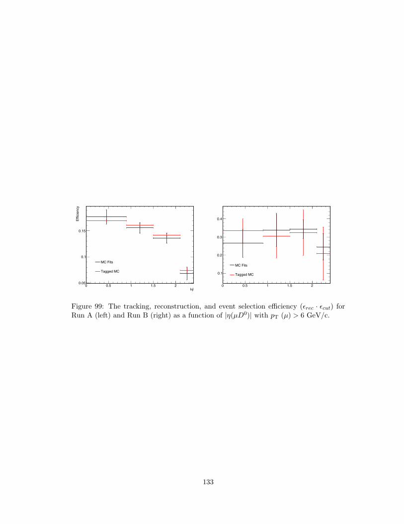
|η|0 0.5 1 1.5 2
Effic
ienc
y
0.05
0.1
0.15
MC Fits
Tagged MC
0 0.5 1 1.5 2
0.1
0.2
0.3
0.4
MC Fits
Tagged MC
Figure 99: The tracking, reconstruction, and event selection efficiency (εrec · εcut) forRun A (left) and Run B (right) as a function of |η(µD0)| with pT (µ) > 6 GeV/c.
133
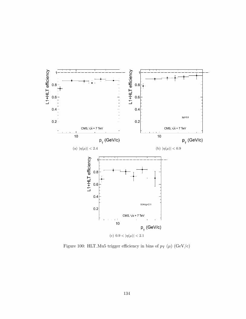
(a) |η(µ)| < 2.4 (b) |η(µ)| < 0.9
(c) 0.9 < |η(µ)| < 2.1
Figure 100: HLT Mu5 trigger efficiency in bins of pT (µ) (GeV/c)
134
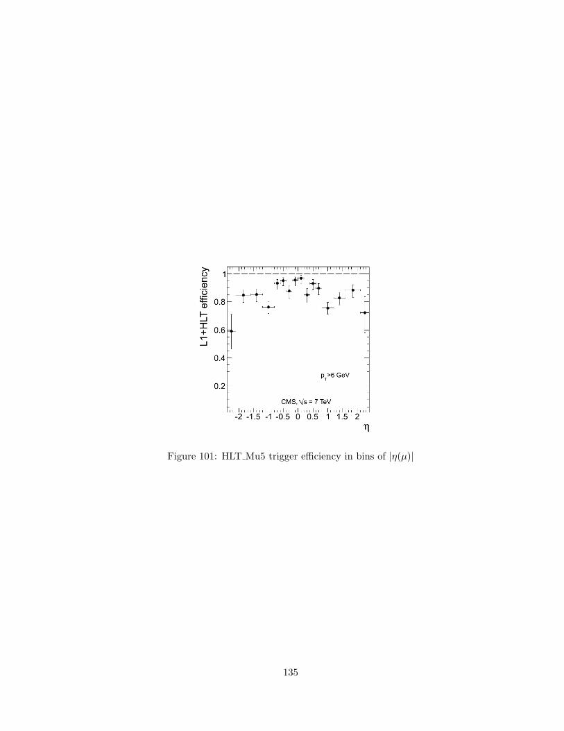
Figure 101: HLT Mu5 trigger efficiency in bins of |η(µ)|
135

(a) |η(µ)| < 2.4 (b) |η(µ)| < 0.9
(c) 0.9 < |η(µ)| < 2.1
Figure 102: HLT Mu15 v1 trigger efficiency in bins of pT (µ) (GeV/c)
136
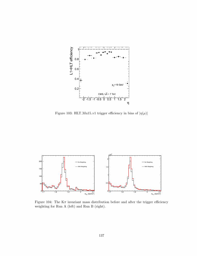
Figure 103: HLT Mu15 v1 trigger efficiency in bins of |η(µ)|
)2 (GeV/cπKm1.7 1.8 1.9 2 2.10
50
100
150
200 No Weighting
With Weighting
)2 (GeV/cπKm1.7 1.8 1.9 2 2.10
0.5
1
1.5
2
310×
No Weighting
With Weighting
Figure 104: The Kπ invariant mass distribution before and after the trigger efficiencyweighting for Run A (left) and Run B (right).
137

7.5 D0 Mass Fits
Similarly to what was already described for the Monte Carlo, the number of µD0 candi-
dates in data is found by fitting the Kπ invariant mass distribution. The distribution is
fit with the double Gaussian function plus a linear background, shown in Equation 14,
and the number of D0 candidates is found from Equation 16. As before, binned likeli-
hood fits are used, and the related χ2 value is shown to have an idea of the goodness-
of-fit. In the Run A dataset, the higher pT bins, which overlap with the Run B dataset,
have low statistics. In these bins the widths, peak position, and ratio of amplitudes are
fixed to those from the equivalent bin in the Run B dataset.
Figure 105 shows the Dπ invariant mass distribution in the data compared to the
Monte Carlo, and shows that the means and the widths of the distributions agree be-
tween data and Monte Carlo. The fits are tuned on the Monte Carlo mass distributions
in order to fix the Gaussian widths. The mass distributions for the data are fit, with the
widths fixed to the values from the Monte Carlo fits. The distribution for pT (µ) > 6
GeV/c and |η(µ)| < 2.4 with the correct charge correlation is shown in Figure 106 before
applying the trigger efficiency weighting to the data, and in Figure 107 after the trigger
efficiency weighting of the data.
(GeV)πKm1.7 1.8 1.9 2 2.10
0.02
0.04
0.06
0.08
0.1
Run A data
MonteCarlo
(GeV)πKm1.7 1.8 1.9 2 2.10
0.02
0.04
0.06
0.08
0.1
Run B data
MonteCarlo
Figure 105: Kπ invariant mass distribution for pT(K,π) > 0.5 GeV/c, and|η(µ,K,π)| < 2.4, pT (µ) > 6 GeV/c for Run A and Monte Carlo (left), and withpT (µ) > 16 GeV/c for Run B and Monte Carlo (right). The data events are weightedby the trigger efficiency. The Monte Carlo is scaled to the luminosity of the data.
138
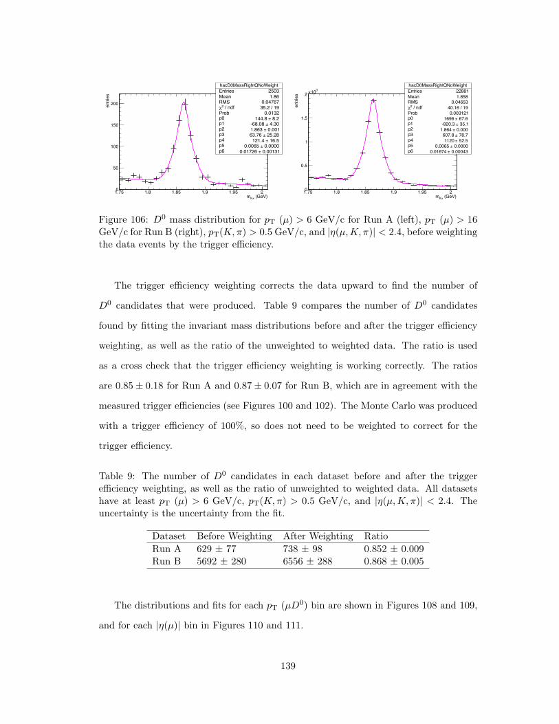
(GeV)πKm1.75 1.8 1.85 1.9 1.95 2
entri
es
0
50
100
150
200
hacD0MassRightQNoWeightEntries 2503Mean 1.86RMS 0.04767
/ ndf 2χ 35.2 / 19Prob 0.0132p0 8.2± 144.8 p1 4.30± -68.08 p2 0.001± 1.863 p3 25.28± 63.76 p4 16.5± 121.4 p5 0.0000± 0.0065 p6 0.00131± 0.01726
(GeV)πKm1.75 1.8 1.85 1.9 1.95 2
entri
es
0
0.5
1
1.5
2310×
hacD0MassRightQNoWeightEntries 22881Mean 1.858RMS 0.04653
/ ndf 2χ 40.16 / 19Prob 0.003121p0 67.6± 1696 p1 35.1± -820.3 p2 0.000± 1.864 p3 78.7± 607.8 p4 52.5± 1120 p5 0.0000± 0.0065 p6 0.00043± 0.01674
Figure 106: D0 mass distribution for pT (µ) > 6 GeV/c for Run A (left), pT (µ) > 16GeV/c for Run B (right), pT(K,π) > 0.5 GeV/c, and |η(µ,K,π)| < 2.4, before weightingthe data events by the trigger efficiency.
The trigger efficiency weighting corrects the data upward to find the number of
D0 candidates that were produced. Table 9 compares the number of D0 candidates
found by fitting the invariant mass distributions before and after the trigger efficiency
weighting, as well as the ratio of the unweighted to weighted data. The ratio is used
as a cross check that the trigger efficiency weighting is working correctly. The ratios
are 0.85± 0.18 for Run A and 0.87± 0.07 for Run B, which are in agreement with the
measured trigger efficiencies (see Figures 100 and 102). The Monte Carlo was produced
with a trigger efficiency of 100%, so does not need to be weighted to correct for the
trigger efficiency.
Table 9: The number of D0 candidates in each dataset before and after the triggerefficiency weighting, as well as the ratio of unweighted to weighted data. All datasetshave at least pT (µ) > 6 GeV/c, pT(K,π) > 0.5 GeV/c, and |η(µ,K,π)| < 2.4. Theuncertainty is the uncertainty from the fit.
Dataset Before Weighting After Weighting RatioRun A 629 ± 77 738 ± 98 0.852 ± 0.009Run B 5692 ± 280 6556 ± 288 0.868 ± 0.005
The distributions and fits for each pT (µD0) bin are shown in Figures 108 and 109,
and for each |η(µ)| bin in Figures 110 and 111.
139

(GeV)πKm1.75 1.8 1.85 1.9 1.95 2
entri
es
0
50
100
150
200
250 / ndf 2χ 35.69 / 19
p0 25.1± 169.5 p1 13.09± -79.64 p2 0.001± 1.863 p3 26.81± 73.31 p4 17.3± 141 p6 0.0012± 0.0175
= 7 TeV sCMS, ) > 6 GeV/cµ(Tp
)| < 2.4µ(η|
97±) = 738 0N(D
(GeV)πKm1.75 1.8 1.85 1.9 1.95 2
entri
es
00.20.40.60.8
11.21.41.61.8
22.2
310× / ndf 2χ 36.82 / 19p0 70.1± 2011 p1 36.4± -972.9 p2 0.000± 1.864 p3 82.1± 684.1 p4 52.1± 1271 p6 0.00039± 0.01708
= 7 TeV sCMS, ) > 16 GeV/cµ(Tp
)| < 2.4µ(η|
288±) = 6555 0N(D
Figure 107: D0 mass distribution for pT (µ) > 6 GeV/c for Run A (left), pT (µ) > 16GeV/c for Run B (right), pT(K,π) > 0.5 GeV/c, and |η(µ,K,π)| < 2.4, after weightingthe data events by the trigger efficiency.
The number of D0 candidates for data and Monte Carlo in each bin are listed in
Table 10.
140

(GeV)πKm1.75 1.8 1.85 1.9 1.95 2
entri
es
0
10
20
30
hacD0MassRightQ_pt5Entries 341Mean 1.86RMS 0.05416
/ ndf 2χ 35.74 / 21Prob 0.02341p0 8.51± 20.79 p1 4.448± -9.631 p2 0.000± 1.865 p3 6.049± 5.942 p4 3.41± 14.38 p5 0.0000± 0.0065 p6 0.000± 0.017
(a) 6 ≤ pT < 11
(GeV)πKm1.75 1.8 1.85 1.9 1.95 2
entri
es0
20
40
60
80
100
hacD0MassRightQ_pt10Entries 944Mean 1.859RMS 0.04273
/ ndf 2χ 25.88 / 21Prob 0.2111p0 14.46± 75.56 p1 7.53± -36.47 p2 0.000± 1.865 p3 12.81± 38.98 p4 6.68± 56.48 p5 0.0000± 0.0065 p6 0.000± 0.017
(b) 11 ≤ pT < 16
(GeV)πKm1.75 1.8 1.85 1.9 1.95 2
entri
es
0
10
20
30
40
50
hacD0MassRightQ_pt15Entries 543Mean 1.862RMS 0.04635
/ ndf 2χ 40.23 / 21Prob 0.00697p0 11.38± 31.98 p1 6.0± -14.9 p2 0.000± 1.865 p3 28.189± 0.761 p4 5.32± 37.97 p5 0.0000± 0.0065 p6 0.000± 0.017
(c) 16 ≤ pT < 20
(GeV)πKm1.75 1.8 1.85 1.9 1.95 2
entri
es
0
10
20
30
40
50
hacD0MassRightQ_pt20Entries 484Mean 1.86RMS 0.05365
/ ndf 2χ 29.25 / 21Prob 0.1082p0 10.75± 42.14 p1 5.61± -20.06 p2 0.000± 1.865 p3 8.82± 16.44 p4 4.23± 23.29 p5 0.0000± 0.0065 p6 0.000± 0.017
(d) 20 ≤ pT < 30
Figure 108: D0 mass distributions in bins of pT (GeV/c) for the 2010A dataset with pT(µ) > 6 GeV/c, pT(K,π) > 0.5 GeV/c and |η(µ,K,π)| < 2.4, weighted by the triggerefficiency.
141
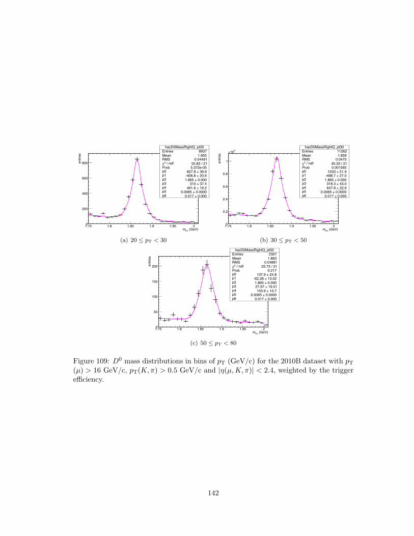
(GeV)πKm1.75 1.8 1.85 1.9 1.95 2
entri
es
0
200
400
600
800
hacD0MassRightQ_pt20Entries 8937Mean 1.855RMS 0.04491
/ ndf 2χ 55.82 / 21Prob 5.372e-05p0 39.9± 827.8 p1 20.6± -406.8 p2 0.000± 1.865 p3 37.4± 310 p4 19.2± 461.6 p5 0.0000± 0.0065 p6 0.000± 0.017
(a) 20 ≤ pT < 30
(GeV)πKm1.75 1.8 1.85 1.9 1.95 2
entri
es0
0.2
0.4
0.6
0.8
1
310×
hacD0MassRightQ_pt30Entries 11262Mean 1.859RMS 0.0475
/ ndf 2χ 45.33 / 21Prob 0.001565p0 51.9± 1033 p1 27.0± -498.7 p2 0.000± 1.865 p3 43.0± 318.3 p4 22.9± 647.8 p5 0.0000± 0.0065 p6 0.000± 0.017
(b) 30 ≤ pT < 50
(GeV)πKm1.75 1.8 1.85 1.9 1.95 2
entri
es
0
50
100
150
200
hacD0MassRightQ_pt50Entries 2307Mean 1.863RMS 0.04881
/ ndf 2χ 25.73 / 21Prob 0.217p0 24.8± 137.9 p1 13.02± -62.28 p2 0.000± 1.865 p3 19.01± 27.97 p4 10.7± 153.9 p5 0.0000± 0.0065 p6 0.000± 0.017
(c) 50 ≤ pT < 80
Figure 109: D0 mass distributions in bins of pT (GeV/c) for the 2010B dataset with pT(µ) > 16 GeV/c, pT(K,π) > 0.5 GeV/c and |η(µ,K,π)| < 2.4, weighted by the triggerefficiency.
142
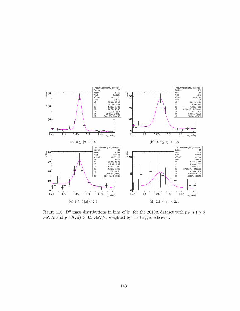
(GeV)πKm1.75 1.8 1.85 1.9 1.95 2
entri
es
0
50
100
150
hacD0MassRightQ_abseta1Entries 1225Mean 1.859RMS 0.04381
/ ndf 2χ 24.65 / 20Prob 0.2153p0 15.05± 83.83 p1 7.85± -40.24 p2 0.000± 1.865 p3 40.33± 24.51 p4 33.7± 103.9 p5 0.0000± 0.0065 p6 0.00155± 0.01182
(a) 0 ≤ |η| < 0.9
(GeV)πKm1.75 1.8 1.85 1.9 1.95 2
entri
es
0
20
40
60
hacD0MassRightQ_abseta2Entries 708Mean 1.86RMS 0.048
/ ndf 2χ 22.83 / 20Prob 0.297p0 13.09± 53.99 p1 6.81± -25.59 p2 0.000± 1.865 p3 1.079e+01± 4.746e-10 p4 4.71± 50.11 p5 0.0000± 0.0065 p6 0.00138± 0.01808
(b) 0.9 ≤ |η| < 1.5
(GeV)πKm1.75 1.8 1.85 1.9 1.95 2
entri
es
0
10
20
30
40hacD0MassRightQ_abseta3
Entries 489Mean 1.862RMS 0.05346
/ ndf 2χ 32.08 / 20Prob 0.0425p0 13.02± 37.83 p1 6.82± -17.39 p2 0.000± 1.865 p3 8.243± 4.664 p4 4.91± 21.61 p5 0.0000± 0.0065 p6 0.00285± 0.02115
(c) 1.5 ≤ |η| < 2.1
(GeV)πKm1.75 1.8 1.85 1.9 1.95 2
entri
es
0
5
10
hacD0MassRightQ_abseta4Entries 81Mean 1.866RMS 0.05636
/ ndf 2χ 19.7 / 20Prob 0.4765p0 5.819± 5.995 p1 3.037± -2.643 p2 0.000± 1.865 p3 1.615e+00± 2.792e-11 p4 1.168± 4.298 p5 0.0000± 0.0065 p6 0.00612± 0.02827
(d) 2.1 ≤ |η| < 2.4
Figure 110: D0 mass distributions in bins of |η| for the 2010A dataset with pT (µ) > 6GeV/c and pT(K,π) > 0.5 GeV/c, weighted by the trigger efficiency.
143
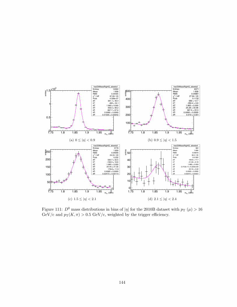
(GeV)πKm1.75 1.8 1.85 1.9 1.95 2
entri
es
0
0.5
1
1.5310×
hacD0MassRightQ_abseta1Entries 12350Mean 1.858RMS 0.04405
/ ndf 2χ 67.69 / 20Prob 4.328e-07p0 46.4± 951.1 p1 24.1± -463 p2 0.000± 1.865 p3 89.2± 406.5 p4 67.9± 897.7 p5 0.0000± 0.0065 p6 0.00042± 0.01305
(a) 0 ≤ |η| < 0.9
(GeV)πKm1.75 1.8 1.85 1.9 1.95 2
entri
es
0
100
200
300
400
500hacD0MassRightQ_abseta2
Entries 6371Mean 1.858RMS 0.04881
/ ndf 2χ 27.84 / 20Prob 0.1132p0 12.7± 589 p1 6.6± -284.4 p2 0.000± 1.865 p3 33.96± 25.28 p4 22.3± 367.5 p5 0.0000± 0.0065 p6 0.001± 0.019
(b) 0.9 ≤ |η| < 1.5
(GeV)πKm1.75 1.8 1.85 1.9 1.95 2
entri
es
0
50
100
150
200
250
hacD0MassRightQ_abseta3Entries 3776Mean 1.859RMS 0.04956
/ ndf 2χ 24.24 / 20Prob 0.232p0 32.5± 330.7 p1 16.8± -158.3 p2 0.000± 1.865 p3 21.35± 24.44 p4 11.9± 178.8 p5 0.0000± 0.0065 p6 0.00114± 0.02473
(c) 1.5 ≤ |η| < 2.1
(GeV)πKm1.75 1.8 1.85 1.9 1.95 2
entri
es
0
10
20
30
40
50
hacD0MassRightQ_abseta4Entries 384Mean 1.856RMS 0.05616
/ ndf 2χ 36.4 / 20Prob 0.01381p0 17.7± 106.8 p1 9.18± -51.94 p2 0.000± 1.865 p3 6.223e+00± 2.412e-11 p4 3.22± 23.19 p5 0.0000± 0.0065 p6 0.00321± 0.02372
(d) 2.1 ≤ |η| < 2.4
Figure 111: D0 mass distributions in bins of |η| for the 2010B dataset with pT (µ) > 16GeV/c and pT(K,π) > 0.5 GeV/c, weighted by the trigger efficiency.
144

Table 10: The number of D0 candidates in each bin. For the 2010A and 2010B columns,the numbers are the results from the invariant mass fits in Run A and Run B data,respectively. For the MC columns they are the number of tagged signal events in theMonte Carlo. All columns have at least pT (µ) > 6 GeV and |η(µ)| < 2.4. Theuncertainty is the uncertainty from the fit.
Bin 2010A 2010B MC MCpT (µ) > 6 GeV pT (µ) > 16 GeV
6 ≤ pT < 11 71 ± 17 – 1245 ± 71 –11 ≤ pT < 16 305 ± 35 – 3955 ± 122 –16 ≤ pT < 20 164 ± 37 0 ± 0 1974 ± 87 0 ± 020 ≤ pT < 30 127 ± 24 2480 ± 101 1755 ± 84 234 ± 3030 ≤ pT < 50 8 ± 0 3281 ± 120 525 ± 46 272 ± 3250 ≤ pT < 80 – 702 ± 55 66 ± 47 45 ± 130 ≤ |η| < 0.9 348 ± 126 3599 ± 282 4880 ± 377 300 ± 880.9 ≤ |η| < 1.5 227 ± 33 1792 ± 135 2584 ± 172 144 ± 391.5 ≤ |η| < 2.1 122 ± 33 1148 ± 96 1901 ± 128 120 ± 182.1 ≤ |η| < 2.4 30 ± 11 138 ± 29 257 ± 47 27 ± 8
145
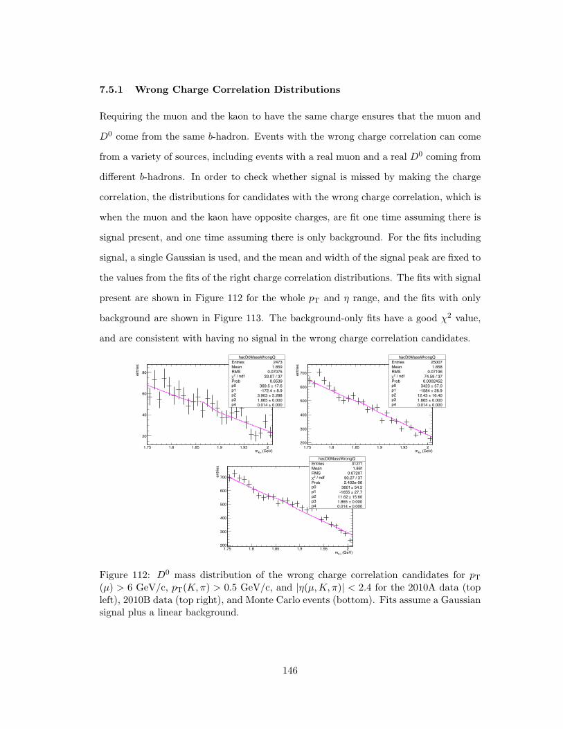
7.5.1 Wrong Charge Correlation Distributions
Requiring the muon and the kaon to have the same charge ensures that the muon and
D0 come from the same b-hadron. Events with the wrong charge correlation can come
from a variety of sources, including events with a real muon and a real D0 coming from
different b-hadrons. In order to check whether signal is missed by making the charge
correlation, the distributions for candidates with the wrong charge correlation, which is
when the muon and the kaon have opposite charges, are fit one time assuming there is
signal present, and one time assuming there is only background. For the fits including
signal, a single Gaussian is used, and the mean and width of the signal peak are fixed to
the values from the fits of the right charge correlation distributions. The fits with signal
present are shown in Figure 112 for the whole pT and η range, and the fits with only
background are shown in Figure 113. The background-only fits have a good χ2 value,
and are consistent with having no signal in the wrong charge correlation candidates.
(GeV)πKm1.75 1.8 1.85 1.9 1.95 2
entri
es
20
40
60
80
hacD0MassWrongQEntries 2473Mean 1.859RMS 0.07075
/ ndf 2χ 33.07 / 37Prob 0.6539p0 17.6± 369.5 p1 8.9± -172.4 p2 5.288± 3.903 p3 0.000± 1.865 p4 0.000± 0.014
(GeV)πKm1.75 1.8 1.85 1.9 1.95 2
entri
es
200
300
400
500
600
700
hacD0MassWrongQEntries 25007Mean 1.858RMS 0.07196
/ ndf 2χ 74.59 / 37Prob 0.0002452p0 57.0± 3423 p1 28.9± -1584 p2 16.40± 12.43 p3 0.000± 1.865 p4 0.000± 0.014
(GeV)πKm1.75 1.8 1.85 1.9 1.95 2
entri
es
200
300
400
500
600
700
hacD0MassWrongQEntries 31271Mean 1.861RMS 0.07207
/ ndf 2χ 90.27 / 37Prob 2.402e-06p0 54.5± 3601 p1 27.7± -1655 p2 15.60± 11.62 p3 0.000± 1.865 p4 0.000± 0.014
Figure 112: D0 mass distribution of the wrong charge correlation candidates for pT(µ) > 6 GeV/c, pT(K,π) > 0.5 GeV/c, and |η(µ,K,π)| < 2.4 for the 2010A data (topleft), 2010B data (top right), and Monte Carlo events (bottom). Fits assume a Gaussiansignal plus a linear background.
146

Table 11 shows the number of D0 candidates for each dataset from fits assuming
a signal in the wrong charge correlation. They are all consistent with having zero D0
candidates.
Table 11: The number of D0 candidates found by the fit assuming a signal for the wrongcharge correlation for pT (µ) > 6 GeV/c and |η(µ)| < 2.4.
Dataset Number of D0 candidatesRun A 14 ± 19Run B 44 ± 58MC 41 ± 55
(GeV)πKm1.75 1.8 1.85 1.9 1.95 2
entri
es
20
40
60
80
hacD0MassWrongQEntries 2473Mean 1.859RMS 0.07075
/ ndf 2χ 23.46 / 20Prob 0.2669p0 1.4± 398.5 p1 0.7± -187.6 p2 0.4± 0 p3 1.4± 0 p4 1.4± 0
(GeV)πKm1.75 1.8 1.85 1.9 1.95 2
entri
es
200
300
400
500
600
700
hacD0MassWrongQEntries 25007Mean 1.858RMS 0.07196
/ ndf 2χ 36.62 / 20Prob 0.013p0 4.5± 3692 p1 2.4± -1726 p2 0.4± 0 p3 1.4± 0 p4 1.4± 0
(GeV)πKm1.75 1.8 1.85 1.9 1.95 2
entri
es
200
300
400
500
600
700
hacD0MassWrongQEntries 31271Mean 1.861RMS 0.07207
/ ndf 2χ 35.88 / 20Prob 0.01588p0 4.4± 3611 p1 2.3± -1654 p2 0.4± 0 p3 1.4± 0 p4 1.4± 0
Figure 113: D0 mass distribution of the wrong charge correlation candidates for pT(µ) > 6 GeV/c, pT(K,π) > 0.5 GeV/c, and |η(µ,K,π)| < 2.4 for the 2010A data (topleft), 2010B data (top right), and Monte Carlo events (bottom). Fits assume backgroundonly.
147

7.6 Systematic Uncertainties
There are several sources of systematic uncertainty in the analysis. They are due to
the uncertainties on other quantities which go into the final result, such as efficiencies.
Some of these uncertainties are bin-dependent, while others are overall uncertainties.
The muon reconstruction and tracking efficiency, hadron tracking efficiency, luminosity,
cut efficiency and trigger efficiency all contribute systematic uncertainties to the cross
section.
There are bin-dependent systematic uncertainties due to the trigger efficiencies and
the statistical error on the selection efficiency. Since the trigger efficiency is applied by
weighting the data events in the invariant mass distribution, the systematic uncertainty
due to the trigger efficiency is found by varying the trigger efficiency up and down by
the statistical errors, and checking the effect on the final cross section in each bin. The
uncertainty for each bin resulting from the error on the trigger efficiency is shown in
Tables 12 and 13.
There is a systematic uncertainty due to the statistical error on the selection ef-
ficiency. The uncertainties are symmetric. This is the dominant uncertainty in this
analysis, due to the low statistics in the Monte Carlo. The uncertainty for each bin
resulting from the error on the selection efficiency is shown in Tables 14 and 15.
There are also systematic uncertainties which are bin-independent, which are due to
the muon reconstruction efficiency, the hadron tracking efficiency, and the luminosity
measurement. The muon and hadron reconstruction and tracking efficiencies are found
from Monte Carlo, which may incorrectly model the efficiencies. The agreement between
the efficiency in Monte Carlo versus data has been studied by other groups in CMS.
The systematic uncertainty due to the muon reconstruction efficiency is 3% [87].
It is evaluated using the tag-and-probe method. The tag-and-probe method exploits
dimuon resonances, such as the J/Ψ. The resonance is reconstructed by putting very
strict requirements on one muon, called the tag, and loose requirements on the second,
called the probe. The usual reconstruction requirements are then placed on the probe
148
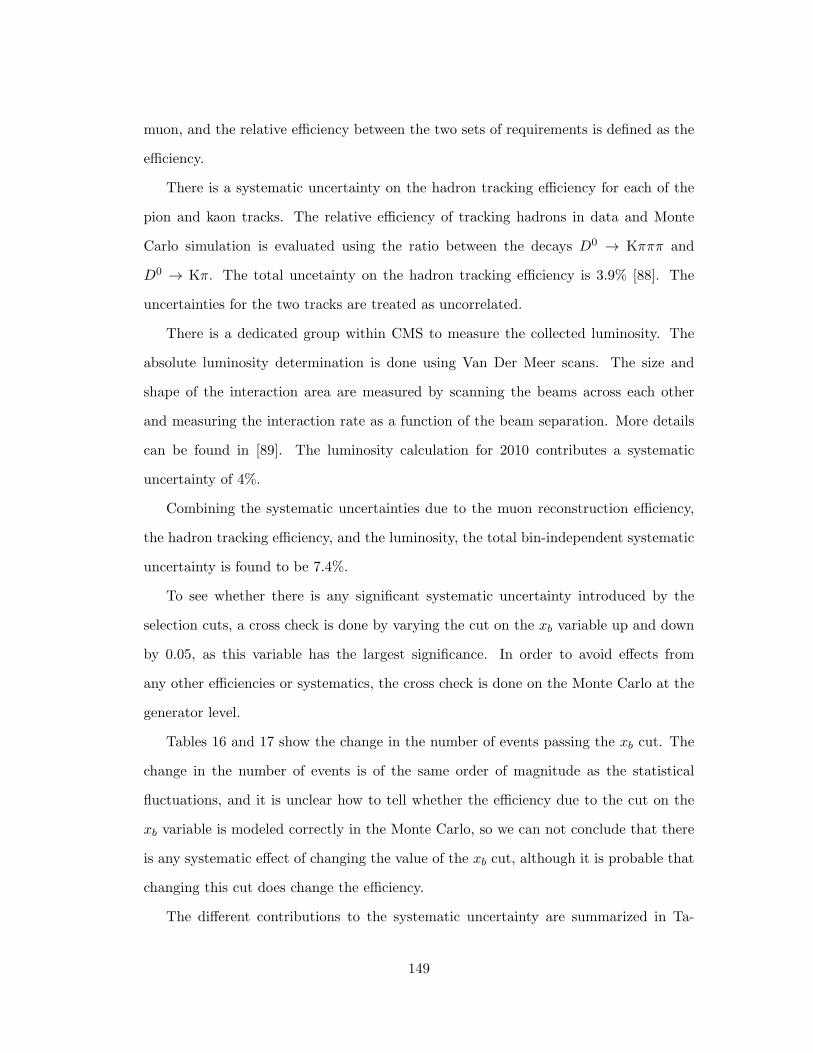
muon, and the relative efficiency between the two sets of requirements is defined as the
efficiency.
There is a systematic uncertainty on the hadron tracking efficiency for each of the
pion and kaon tracks. The relative efficiency of tracking hadrons in data and Monte
Carlo simulation is evaluated using the ratio between the decays D0 → Kπππ and
D0 → Kπ. The total uncetainty on the hadron tracking efficiency is 3.9% [88]. The
uncertainties for the two tracks are treated as uncorrelated.
There is a dedicated group within CMS to measure the collected luminosity. The
absolute luminosity determination is done using Van Der Meer scans. The size and
shape of the interaction area are measured by scanning the beams across each other
and measuring the interaction rate as a function of the beam separation. More details
can be found in [89]. The luminosity calculation for 2010 contributes a systematic
uncertainty of 4%.
Combining the systematic uncertainties due to the muon reconstruction efficiency,
the hadron tracking efficiency, and the luminosity, the total bin-independent systematic
uncertainty is found to be 7.4%.
To see whether there is any significant systematic uncertainty introduced by the
selection cuts, a cross check is done by varying the cut on the xb variable up and down
by 0.05, as this variable has the largest significance. In order to avoid effects from
any other efficiencies or systematics, the cross check is done on the Monte Carlo at the
generator level.
Tables 16 and 17 show the change in the number of events passing the xb cut. The
change in the number of events is of the same order of magnitude as the statistical
fluctuations, and it is unclear how to tell whether the efficiency due to the cut on the
xb variable is modeled correctly in the Monte Carlo, so we can not conclude that there
is any systematic effect of changing the value of the xb cut, although it is probable that
changing this cut does change the efficiency.
The different contributions to the systematic uncertainty are summarized in Ta-
149

ble 18. The uncertainties are combined by adding them in quadrature.
150
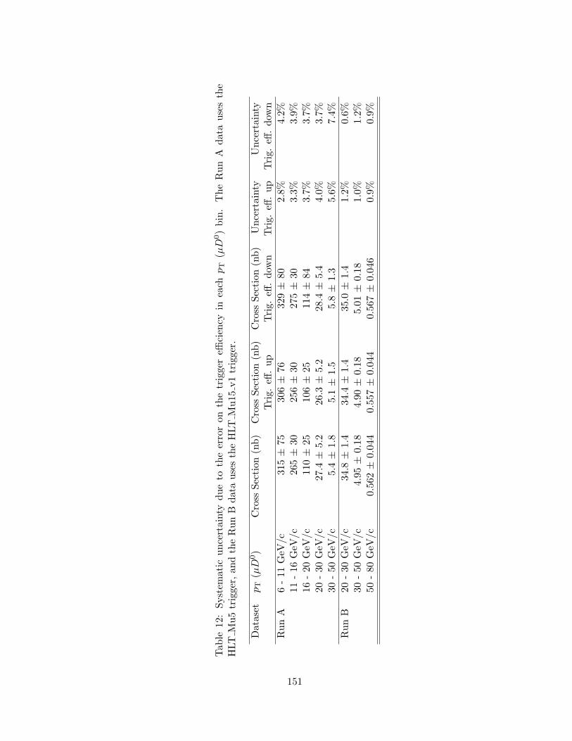
Tab
le12:Systematic
uncertaintydueto
theerroron
thetriggereffi
ciency
ineach
p T(µD
0)bin.TheRunA
datausesthe
HLT
Mu5trigger,
andtheRunB
datausestheHLT
Mu15
v1trigger.
Dataset
p T(µD
0)
Cross
Section
(nb)
Cross
Section
(nb)
Cross
Section
(nb)
Uncertainty
Uncertainty
Trig.
eff.up
Trig.
eff.dow
nTrig.
eff.up
Trig.
eff.dow
nRunA
6-11
GeV
/c31
5±
7530
6±
7632
9±
802.8%
4.2%
11-16
GeV
/c26
5±
3025
6±
3027
5±
303.3%
3.9%
16-20
GeV
/c11
0±
2510
6±
2511
4±
843.7%
3.7%
20-30
GeV
/c27
.4±
5.2
26.3
±5.2
28.4
±5.4
4.0%
3.7%
30-50
GeV
/c5.4±
1.8
5.1±
1.5
5.8±
1.3
5.6%
7.4%
RunB
20-30
GeV
/c34
.8±
1.4
34.4
±1.4
35.0
±1.4
1.2%
0.6%
30-50
GeV
/c4.95
±0.18
4.90
±0.18
5.01
±0.18
1.0%
1.2%
50-80
GeV
/c0.562±
0.044
0.557±
0.044
0.56
7±
0.04
60.9%
0.9%
151
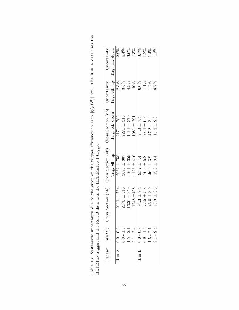
Tab
le13:Systematic
uncertaintydueto
theerroron
thetriggereffi
ciency
ineach
|η(µD
0)|
bin.
TheRunA
datausesthe
HLT
Mu5trigger,
andtheRunB
datausestheHLT
Mu15
v1trigger.
Dataset
|η(µD
0)|
Cross
Section
(nb)
Cross
Section
(nb)
Cross
Section
(nb)
Uncertainty
Uncertainty
Trig.
eff.up
Trig.
eff.dow
nTrig.
eff.up
Trig.
eff.dow
nRunA
0.0-0.9
2111
±76
420
62±
758
2171
±78
22.3%
2.9%
0.9-1.5
2175
±31
620
98±
307
2271
±31
63.5%
4.4%
1.5-2.1
1326
±35
912
61±
359
1414
±37
04.9%
6.6%
2.1-2.4
1248
±45
811
23±
416
1081
±29
110
%13
%RunB
0.0-0.9
94.3
±7.4
93.7
±7.4
95.0
±7.4
0.6%
0.7%
0.9-1.5
77.5
±5.8
76.6
±5.8
78.4
±6.3
1.1%
1.2%
1.5-2.1
46.5
±3.9
46.0
±3.9
47.2
±3.9
1.2%
1.4%
2.1-2.4
17.3
±3.6
15.8
±3.4
15.4
±2.0
8.7%
11%
152

Table 14: Systematic uncertainty due to the statistical error on the selection efficiencyfor Run A with pT (µ) > 6 GeV/c and |η(µ)| < 2.4.
Bin Generated Tagged Efficiency Syst. UncertaintypT (µD0) 6 - 11 GeV/c 30422 1269 (4.2 ± 0.1)% 2.5%
11 - 16 GeV/c 18775 4008 (21 ± 0.3)% 1.4%16 - 20 GeV/c 5760 1994 (35 ± 0.8)% 2.3%20 - 30 GeV/c 4119 1771 (43 ± 1)% 2.3%30 - 50 GeV/c 1005 511 (51 ± 2)% 3.9%30 - 50 GeV/c 119 57 (48 ± 6)% 12.5%
|η(µD0)| 0.0 - 0.9 27610 4684 (17 ± 0.2)% 1.2%0.9 - 1.5 16592 2673 (16 ± 0.3)% 1.9%1.5 - 2.1 13961 1982 (14 ± 0.3)% 2.1%2.1 - 2.4 3759 279 (7 ± 0.4)% 5.7%
Table 15: Systematic uncertainty due to the statistical error on the selection efficiencyfor Run B with pT (µ) > 16 GeV/c and |η(µ)| < 2.4.
Bin Generated Fit Efficiency Syst. UncertaintypT (µD0) 16 - 20 GeV/c 879 231 (27 ± 2)% 7.4%
20 - 30 GeV/c 559 262 (47 ± 3)% 6.4%30 - 50 GeV/c 89 39 (44 ± 7)% 15.9%
|η(µD0)| 0.0 - 0.9 824 275 (33 ± 2)% 6.7%0.9 - 1.5 425 129 (30 ± 3)% 9.4%1.5 - 2.1 349 113 (32 ± 3)% 14.3%2.1 - 2.4 110 23 (21 ± 4)% 19.0%
153
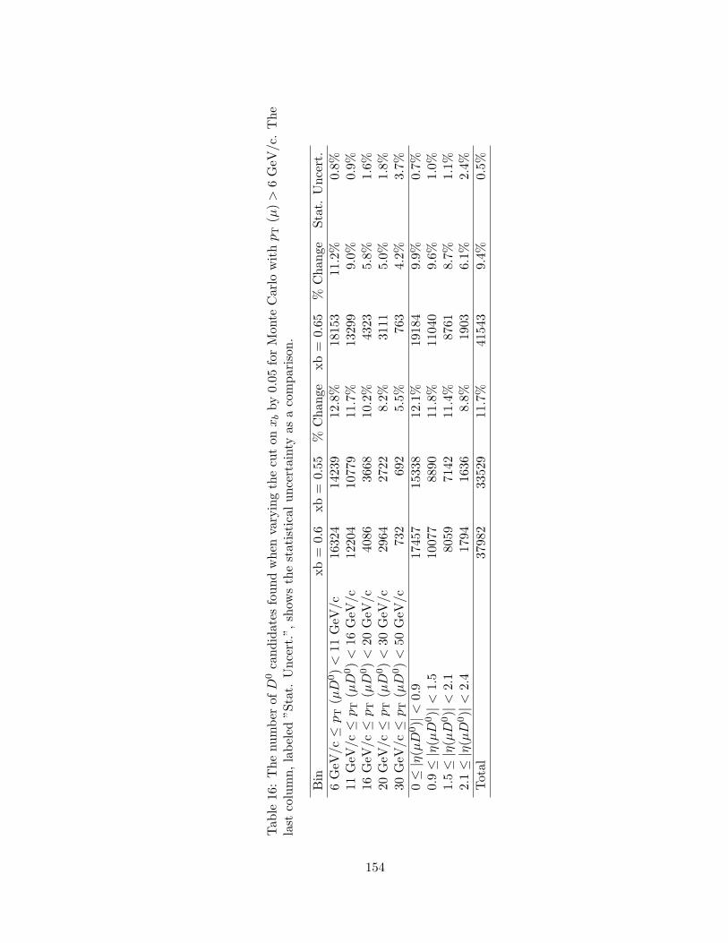
Tab
le16:Thenu
mber
ofD
0candidates
foundwhen
varyingthecuton
xbby
0.05
forMon
teCarlo
withp T
(µ)>
6GeV
/c.The
last
column,labeled
”Stat.
Uncert.”,show
sthestatisticaluncertaintyas
acomparison
.
Bin
xb=
0.6
xb=
0.55
%Chan
gexb
=0.65
%Chan
geStat.
Uncert.
6GeV
/c≤
p T(µD
0)<
11GeV
/c16
324
14239
12.8%
1815
311
.2%
0.8%
11GeV
/c≤
p T(µD
0)<
16GeV
/c12
204
10779
11.7%
1329
99.0%
0.9%
16GeV
/c≤
p T(µD
0)<
20GeV
/c40
8636
6810
.2%
4323
5.8%
1.6%
20GeV
/c≤
p T(µD
0)<
30GeV
/c29
6427
228.2%
3111
5.0%
1.8%
30GeV
/c≤
p T(µD
0)<
50GeV
/c73
269
25.5%
763
4.2%
3.7%
0≤
|η(µD
0)|<
0.9
17457
15338
12.1%
1918
49.9%
0.7%
0.9≤
|η(µD
0)|<
1.5
10077
8890
11.8%
1104
09.6%
1.0%
1.5≤
|η(µD
0)|<
2.1
8059
7142
11.4%
8761
8.7%
1.1%
2.1≤
|η(µD
0)|<
2.4
1794
1636
8.8%
1903
6.1%
2.4%
Total
37982
33529
11.7%
4154
39.4%
0.5%
154

Tab
le17:Thenu
mber
ofD
0candidates
foundwhen
varyingthecuton
xbby
0.05
forMon
teCarlo
withp T
(µ)>
16GeV
/c.
Thelast
column,labeled
”Stat.
Uncert.”,show
sthestatisticaluncertaintyas
acomparison
.
Bin
xb=
0.6
xb=
0.55
%Chan
gexb
=0.65
%Chan
geStat.
Uncert.
20GeV
/c≤
p T(µD
0)<
30GeV
/c62
558
46.56
%65
75.12
%4.0%
30GeV
/c≤
p T(µD
0)<
50GeV
/c41
339
34.84
%43
04.12
%4.9%
50GeV
/c≤
p T(µD
0)<
80GeV
/c57
545.26
%59
3.51
%13
.3%
0≤
|η(µD
0)|<
0.9
606
569
6.1%
633
4.5%
4.0%
0.9≤
|η(µD
0)|<
1.5
294
280
4.76
%31
15.78
%5.8%
1.5≤
|η(µD
0)|<
2.1
248
230
7.26
%26
15.24
%6.3%
2.1≤
|η(µD
0)|<
2.4
6360
4.76
%66
4.76
%12
.6%
Total
1225
1152
5.96
%12
864.98
%2.9%
155

Table 18: Systematic uncertainties on the cross section.
Source Cross section uncertaintyTrigger efficiency 1% - 13%Selection efficiency 1% - 19%Muon reconstruction efficiency 3%Hadron tracking efficiency (x2) 3.9%All Efficiencies 6.8% - 24.4%Luminosity 4%Branching Ratio 5.3%
156
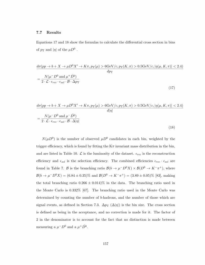
7.7 Results
Equations 17 and 18 show the formulas to calculate the differential cross section in bins
of pT and |η| of the µD0 .
dσ(pp → b+X → µD0X ′ → Kπ, pT(µ) > 6GeV/c, pT(K,π) > 0.5GeV/c, |η(µ,K,π)| < 2.4)
dpT
=N(µ−D0 and µ+D0)
2 · L · εrec · εsel · B ·∆pT
(17)
dσ(pp → b+X → µD0X ′ → Kπ, pT(µ) > 6GeV/c, pT(K,π) > 0.5GeV/c, |η(µ,K,π)| < 2.4)
d|η|
=N(µ−D0 and µ−D0)
2 · L · εrec · εsel · B ·∆|η|
(18)
N(µD0) is the number of observed µD0 candidates in each bin, weighted by the
trigger efficiency, which is found by fitting the Kπ invariant mass distribution in the bin,
and are listed in Table 10. L is the luminosity of the dataset. εrec is the reconstruction
efficiency and εsel is the selection efficiency. The combined efficiencies εrec · εsel are
found in Table 7. B is the branching ratio B(b → µ−D0X) × B(D0 → K−π+), where
B(b → µ−D0X) = (6.84 ± 0.35)% and B(D0 → K−π+) = (3.89 ± 0.05)% [83], making
the total branching ratio 0.266 ± 0.014)% in the data. The branching ratio used in
the Monte Carlo is 0.332% [67]. The branching ratio used in the Monte Carlo was
determined by counting the number of b-hadrons, and the number of those which are
signal events, as defined in Section 7.3. ∆pT (∆|η|) is the bin size. The cross section
is defined as being in the acceptance, and no correction is made for it. The factor of
2 in the denominator is to account for the fact that no distinction is made between
measuring a µ−D0 and a µ+D0.
157

Ideally the differential cross section should be presented as a function of the pT and
|η| of the b-hadron, but the b-hadron can not be fully reconstructed, due to at least
the missing neutrino. This would also allow a more direct comparison to measurements
from other experiments. Since the Monte Carlo sample has the requirement for a muon
with at least pT > 5 GeV/c, it is not possible to do the unfolding. A Monte Carlo
sample without any cuts on the pT and |η| of the particles would be required to unfold
to the full region. New Monte Carlo samples could not be generated since the data was
processed in an old CMSSW version, which is no longer available.
As an example and cross check, here I follow one bin through the entire analysis
sequence in the Monte Carlo. For this purpose I use the bin with pT (µ) from 16-
20 GeV/c. First, using the generator information, I follow the number of true signal
events through each step in the analysis. At the end I compare the true number of
tagged signal events remaining with the number found from fitting the Kπ invariant
mass distribution.
Before any event selection, there are 6531 generated signal events. 5760 of these
events are in the acceptance (see Table 14), which means that the µ, K and π have
|η| < 2.4. After all of the selection cuts, there are 1994 tagged Monte Carlo signal
events remaining. From the fit of the Kπ invariant mass distribution, there are 1974 ±
87 D0 candidates, which is consistent with the true value of 1994 tagged Monte Carlo
signal events.
To calculate the differential cross section for the Monte Carlo, N(µD0) is the
number of generated signal events in the acceptance of pT(µ) > 6GeV/c, pT(K,π) >
0.5GeV/c, and|η(µ,K,π)| < 2.4 and in the particular bin. In Equation 17, the efficiency
ε is equal to 1 by definition. The luminosity of the Monte Carlo sample is 1.23 pb−1.
The cross section in Monte Carlo for the bin 16 GeV/c ≤ pT(µD0) < 20 GeV/c is shown
below, and is also shown in Table 19. The branching ratio of b → µD0X → Kπ in the
Monte Carlo is 0.00332, as described above, and the pT bin width ∆pT is 4 GeV/c.
158
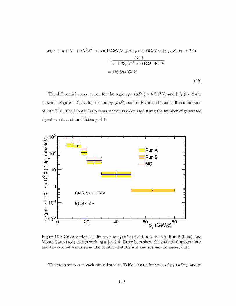
σ(pp → b+X → µD0X ′ → Kπ,16GeV/c ≤ pT(µ) < 20GeV/c, |η(µ,K,π)| < 2.4)
=5760
2 · 1.23pb−1 · 0.00332 · 4GeV
= 176.3nb/GeV
(19)
The differential cross section for the region pT (µD0) > 6 GeV/c and |η(µ)| < 2.4 is
shown in Figure 114 as a function of pT (µD0), and in Figures 115 and 116 as a function
of |η(µD0)|. The Monte Carlo cross section is calculated using the number of generated
signal events and an efficiency of 1.
(GeV/c) T
p0 20 40 60 80
(nb/
GeV
)T
X’)
/ dp
0 Dµ
→ b
+X
→(p
p σd -210
-110
1
10
210
310
Run ARun BMC
Run ARun BMC
= 7 TeV sCMS,
)| < 2.4µ(η|
Figure 114: Cross section as a function of pT(µD0) for Run A (black), Run B (blue), andMonte Carlo (red) events with |η(µ)| < 2.4. Error bars show the statistical uncertainty,and the colored bands show the combined statistical and systematic uncertainty.
The cross section in each bin is listed in Table 19 as a function of pT (µD0), and in
159
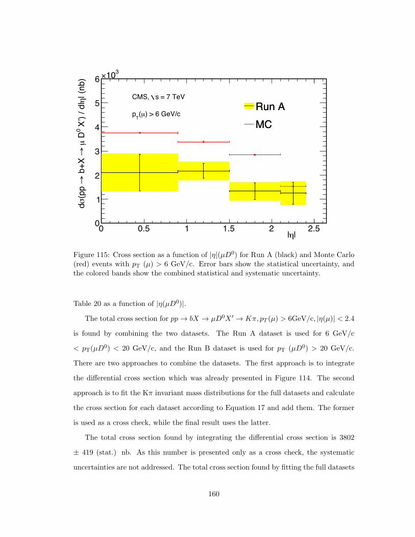
| η|0 0.5 1 1.5 2 2.5
| (nb
)η
X’)
/ d|
0 Dµ
→ b
+X
→(p
p σd
0
1
2
3
4
5
6310×
Run AMCRun AMC
= 7 TeV sCMS,
) > 6 GeV/cµ(Tp
Figure 115: Cross section as a function of |η|(µD0) for Run A (black) and Monte Carlo(red) events with pT (µ) > 6 GeV/c. Error bars show the statistical uncertainty, andthe colored bands show the combined statistical and systematic uncertainty.
Table 20 as a function of |η(µD0)|.
The total cross section for pp → bX → µD0X ′ → Kπ, pT (µ) > 6GeV/c, |η(µ)| < 2.4
is found by combining the two datasets. The Run A dataset is used for 6 GeV/c
< pT(µD0) < 20 GeV/c, and the Run B dataset is used for pT (µD0) > 20 GeV/c.
There are two approaches to combine the datasets. The first approach is to integrate
the differential cross section which was already presented in Figure 114. The second
approach is to fit the Kπ invariant mass distributions for the full datasets and calculate
the cross section for each dataset according to Equation 17 and add them. The former
is used as a cross check, while the final result uses the latter.
The total cross section found by integrating the differential cross section is 3802
± 419 (stat.) nb. As this number is presented only as a cross check, the systematic
uncertainties are not addressed. The total cross section found by fitting the full datasets
160
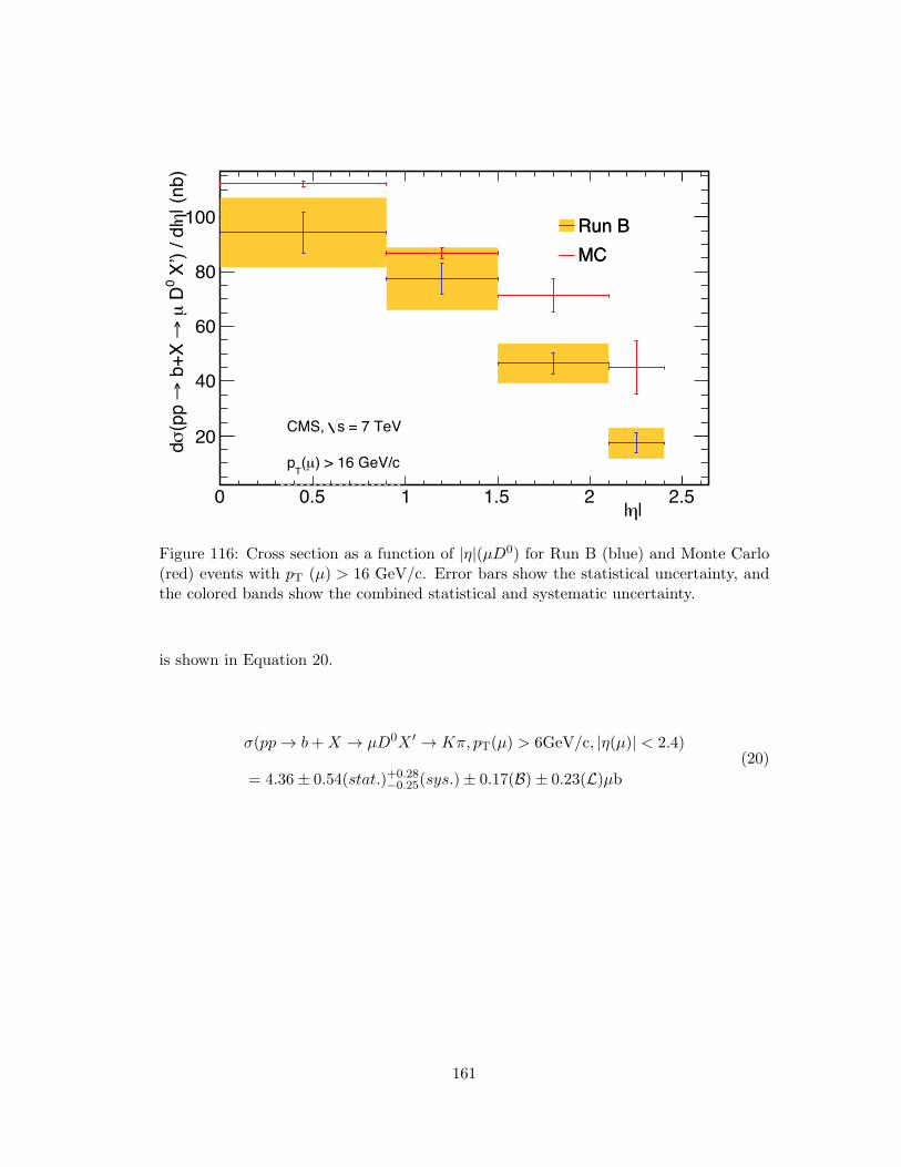
| η|0 0.5 1 1.5 2 2.5
| (nb
)η
X’)
/ d|
0 Dµ
→ b
+X
→(p
p σd 20
40
60
80
100 Run BMCRun BMC
= 7 TeV sCMS,
) > 16 GeV/cµ(Tp
Figure 116: Cross section as a function of |η|(µD0) for Run B (blue) and Monte Carlo(red) events with pT (µ) > 16 GeV/c. Error bars show the statistical uncertainty, andthe colored bands show the combined statistical and systematic uncertainty.
is shown in Equation 20.
σ(pp → b+X → µD0X ′ → Kπ, pT(µ) > 6GeV/c, |η(µ)| < 2.4)
= 4.36± 0.54(stat.)+0.28−0.25(sys.)± 0.17(B)± 0.23(L)µb
(20)
161

Tab
le19
:Thecrosssectionin
each
p T(µD
0)bin.
Bin
2010
A20
10B
Mon
teCarlo
MC15
6≤
p T<
11315.3±
75.5
(stat.)±
31.4
(sys.)
–74
5.0±
4.3(stat.)
–11
≤p T
<16
264.6±
30.4
(stat.)±
26.0
(sys.)
–46
0.0±
3.4(stat.)
–16
≤p T
<20
109.7±
24.7
(stat.)±
10.8
(sys.)
–17
6.3±
2.3(stat.)
176.3±
17.0
(stat.)
20≤
p T<
3027.4
±5.2(stat.)±
2.8(sys.)
34.8
±1.4(stat.)±
3.9(sys.)
50.4
±0.8(stat.)
50.4
±1.7(stat.)
30≤
p T<
505.4±
1.8(stat.)±
0.6(sys.)
5.0±
0.2(stat.)±
0.6(sys.)
6.2±
0.2(stat.)
6.2±
0.3(stat.)
50≤
p T<
80–
0.56
±0.04
(stat.)±
0.11
(sys.)
0.49
±0.04
(stat.)
0.49
±0.05
(stat.)
162
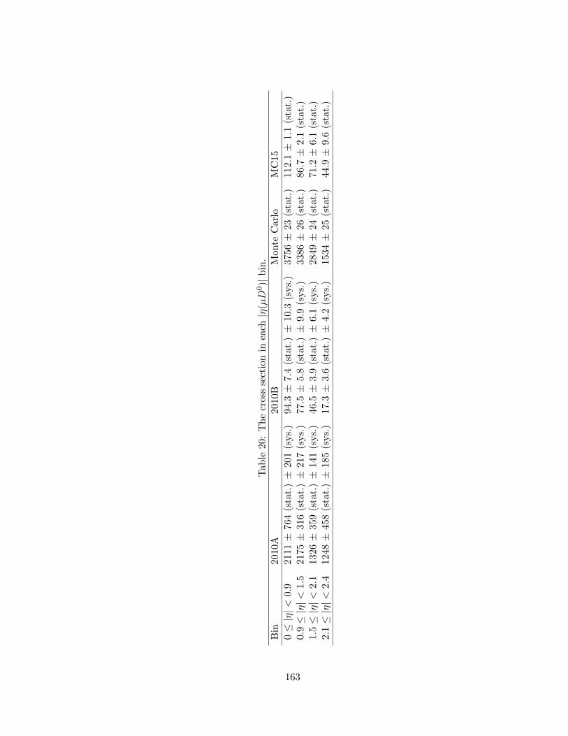
Tab
le20
:Thecrosssectionin
each
|η(µD
0)|bin.
Bin
2010
A20
10B
Mon
teCarlo
MC15
0≤
|η|<
0.9
2111
±76
4(stat.)±
201(sys.)
94.3
±7.4(stat.)±
10.3
(sys.)
3756
±23
(stat.)
112.1±
1.1(stat.)
0.9≤
|η|<
1.5
2175
±31
6(stat.)±
217(sys.)
77.5
±5.8(stat.)±
9.9(sys.)
3386
±26
(stat.)
86.7
±2.1(stat.)
1.5≤
|η|<
2.1
1326
±35
9(stat.)±
141(sys.)
46.5
±3.9(stat.)±
6.1(sys.)
2849
±24
(stat.)
71.2
±6.1(stat.)
2.1≤
|η|<
2.4
1248
±45
8(stat.)±
185(sys.)
17.3
±3.6(stat.)±
4.2(sys.)
1534
±25
(stat.)
44.9
±9.6(stat.)
163
8 Conclusion
Measuring the b production cross section provides a good test of pQCD. Since b-quarks
constitute a significant source of background for many future studies it is important to
have a good understanding of their production. Because of the reliance of this analysis
on the reconstruction of secondary vertices, it is essential to have a reliable tracking
detector with good resolution. The detector is exposed to considerable amounts of
radiation, and the effects of the radiation must be understood.
Several measurements of the current CMS barrel pixel sensors were performed in
order to evaluate their performance in the harsh radiation environment of the LHC.
These measurements were charge collection efficiency measurements to measure the
amount of signal lost, detection efficiency measurements, and interpixel capacitance
measurements. The goals of the measurements were to determine the operational limits
of the sensors, and their suitability for use in the CMS Phase 1 Upgrade pixel detector.
In addition, high voltage tests were performed on single-sided sensors, which are cheaper
to produce, to investigate their feasibility for future upgrades.
The different measurements performed on the current CMS barrel pixel sensors show
that they work remarkably well even at high fluences. In particular, the charge collection
efficiency measurements show that a significant amount of charge can be collected even
after fluences of more than 1015 neq/cm2 , provided that a high bias voltage can be
applied. This confirms that the sensors will survive past the design requirement of
250 fb−1 of integrated luminosity. The measurements in this dissertation led in part
to the decision to maintain the same sensor material and design for the CMS Phase I
Upgrade pixel detector.
The main concern prompting the Phase I Upgrade pixel detector is the performance
the readout chip with increased luminosity, where the main problems will be filling the
buffers on the chip. The amount of signal collected will gradually decline with the
radiation damage, with the limiting factors in the bias voltage being the cables and
164

connectors to supply the voltage to the sensors. The measurements also show that the
lifetime of the sensors is not limited by the amount of charge collected, but by the
reduction in the spatial resolution due to the increasing bias voltage needed.
In addition to the measurements on the silicon pixel sensors, a measurement of
the bb cross section at a center-of-mass energy of√s = 7 TeV using the decay chain
b → µD0X, D0 → Kπ has been presented. The measurement is based on an integrated
luminosity of ∼25 pb−1 taken during 2010. The total cross section in the acceptance is
σ(pp → b +X → µD0X ′, pT(µ) > 6GeV/c, pT(K,π) > 0.5GeV/c, |η(µ,K,π)| < 2.4) =
4.36± 0.54(stat.)+0.28−0.25(sys.)± 0.17(B)± 0.23(L)µb.
Comparison with the LO PYTHIA Monte Carlo QCD sample shows that it over-
estimates the cross section by approximately a factor of 2. This is consistent with
observations from other analyses [6]. The measurement is limited by the systematic
uncertainty from the selection efficiencies, which is very large due to the limited statis-
tics in the Monte Carlo sample. A similar analysis in CMS showed that the difference
between the data and theoretical predictions are much smaller once NLO effects are
included [15]. This reflects the fact that NLO processes such as flavor excitation and
gluon splittings are important at the LHC.
ATLAS and LHCb have also made measurements of the inclusive bb cross section.
The ATLAS measurement uses the final state µD∗X, with the D∗ reconstructed with
the decay chain D∗ → πD0, D0 → Kπ. The ATLAS results are compared to theoretical
predictions from POWHEG+PYTHIA, POWHEG+Herwig, and MC@NLO. In all cases
the data is higher than the theoretical predictions, although barely consistent within
the errors. In LHCb, the same final states as in this dissertation, namely, B → µD0X,
D0 → Kπ, are used. The LHCb measurements are presented only as a function of η,
but are consistent with the theoretical predictions from FONLL. Until now there has
been no equivalent measurement published by CMS.
The measurement presented in this dissertation can not be directly compared to
those of the other LHC experiments without first unfolding to the b-hadron and extrap-
165

olating to the full phase space. This would require a significant effort to produce new
Monte Carlo samples, which was not possible in the time frame for this dissertation.
A very general comparison can be made between this measurement and the ones
from ATLAS and LHCb by looking at the relative agreement between each measure-
ment and the Monte Carlo predictions, and the differences between the Monte Carlo
generators. As seen in Figure 68, ATLAS finds the POWHEG+PYTHIA underesti-
mates the cross section by approximately a factor of 2. The CMS measurement using
the prelT also finds that the POWHEG+PYTHIA underestimates the cross section by
about a factor of 1.5 (see Figure 70), and that PYTHIA overestimates the cross section
by approximately a factor of 2 (see Figure 69). LHCb compares their measurement
with the FONLL predictions and finds the predictions to be consistent with the data,
as shown in Figure 67. The CMS prelT measurement also finds the FONLL predictions
to be consistent with the data. In conclusion, it appears that the measurement pre-
sented in this dissertation is consistent with the measurements from ATLAS and LHCb,
although it should be stressed that this is a very indirect comparison.
An interesting continuation of this analysis would be to compare with the cross
section measured by the LHCb experiment, using the same final states. LHCb measures
in the forward region (|η| > 2), where CMS suffers from low efficiencies, making this a
challenging task which was not possible to cover in the scope of this dissertation.
166

References
[1] Michael Moll. Radiation damage in silicon particle detectors – microscopic defects
and macroscopic properties. PhD thesis, Universitat Hamburg, 1999.
[2] CERN. http://home.web.cern.ch/.
[3] The CMS Collaboration. The CMS experiment at the CERN LHC. Journal of
Instrumentation, 3(8):S08004, 2008.
[4] The CMS Collaboration. Tracking and primary vertex results in first 7 tev colli-
sions. CMS PAS TRK-10-005, 2010.
[5] O. Koybasi, K. Arndt, G. Bolla, D. Bortoletto, P. Merkel, and I. Shipsey. Assembly
and qualification procedures of cms forward pixel detector modules. Nucl. Instrum.
Meth. A, 638:55–62, 2011.
[6] Lea Caminada. Study of the Inclusive Beauty Production at CMS and Construc-
tion and Commissioning of the CMS Pixel Barrel Detector. PhD thesis, Eid-
genossische Technische Hochschule Zurich, 2010.
[7] Y. Allkofer, C. Amsler, D. Bortoletto, V. Chiochia, L. Cremaldi, S. Cucciarelli,
A. Dorokhov, C. Hormann, R. Horisberger, D. Kim, M. Konecki, D. Kotlin-
ski, K. Prokofiev, C. Regenfus, T. Rohe, D.A. Sanders, S. Son, M. Swartz, and
T. Speer. Design and performance of the silicon sensors for the CMS barrel pixel
detector. Nuclear Instruments and Methods in Physics Research Section A: Ac-
celerators, Spectrometers, Detectors and Associated Equipment, 584(1):25 – 41,
2008.
[8] C Amsler, K Bosiger, V Chiochia, W Erdmann, K Gabathuler, R Horisberger,
S Konig, D Kotlinski, R Maier, B Meier, Hp Meyer, A Rizzi, P Robmann, S Scherr,
A Schmidt, S Steiner, and S Streuli. Mechanical design and material budget of
the cms barrel pixel detector. Journal of Instrumentation, 4(05):P05003, 2009.
167

[9] Alexandra Junkes. Influence of radiation induced defect clusters on silicon particle
detectors. PhD thesis, Universitat Hamburg, 2011.
[10] V Eremin, E Verbitskaya, and Z Li. The origin of double peak electric field distri-
bution in heavily irradiated silicon detectors. Nuclear Instruments and Methods
in Physics Research Section A: Accelerators, Spectrometers, Detectors and Asso-
ciated Equipment, 476(3):556 – 564, 2002.
[11] CDF Collaboration. Measurements of bottom anti-bottom azimuthal produc-
tion correlations in proton-antiproton collisions at√s = 1.8 TeV. Phys. Rev. D,
71(9):092001, May 2005.
[12] CDF Collaboration. Measurement of the b-hadron production cross section using
decays to µ−D0x final states in pp collisions at√s = 1.96 TeV. Phys. Rev. D,
79(9):092003, 2009.
[13] The LHCb Collaboration. Measurement of σ(pp → bbX) at√s = 7 TeV in the
forward region. Physics Letters B, 694:209–216, 2010.
[14] The ATLAS Collaboration. Measurement of the b-hadron production cross section
using decays to final states in pp collisions at with the atlas detector. Nuclear
Physics B, 864(3):341 – 381, 2012.
[15] L. Caminada, W. Erdmann, U. Langenegger, V. Zhukov, D. Troendle, S. Wayand,
A. Bean, and G. Tinti. Inclusive b → µX cross section measurement at 7 TeV.
CMS AN-10-346, 2010.
[16] S. Glashow. Partial-symmetries of weak interactions. Nuclear Physics, 22(4):579
– 588, 1961.
[17] S. Weinberg. A model of leptons. Phys. Rev. Lett., 19:1264–1266, Nov 1967.
168

[18] Abdus Salam. Weak and electromagnetic interactions. Originally printed in
*Svartholm: Elementary Particle Theory, Proceedings Of The Nobel Symposium
Held 1968 At Lerum, Sweden*, Stockholm 1968, 367-377.
[19] S. L. Glashow, J. Iliopoulos, and L. Maiani. Weak interactions with lepton-hadron
symmetry. Phys. Rev. D, 2:1285–1292, Oct 1970.
[20] J. J. Aubert, U. Becker, P. J. Biggs, J. Burger, M. Chen, G. Everhart, P. Gold-
hagen, J. Leong, T. McCorriston, T. G. Rhoades, M. Rohde, Samuel C. C. Ting,
Sau Lan Wu, and Y. Y. Lee. Experimental observation of a heavy particle j.
Phys. Rev. Lett., 33:1404–1406, Dec 1974.
[21] J. E. Augustin, A. M. Boyarski, M. Breidenbach, F. Bulos, J. T. Dakin, G. J.
Feldman, G. E. Fischer, D. Fryberger, G. Hanson, B. Jean-Marie, R. R. Larsen,
V. Luth, H. L. Lynch, D. Lyon, C. C. Morehouse, J. M. Paterson, M. L. Perl,
B. Richter, P. Rapidis, R. F. Schwitters, W. M. Tanenbaum, F. Vannucci, G. S.
Abrams, D. Briggs, W. Chinowsky, C. E. Friedberg, G. Goldhaber, R. J. Holle-
beek, J. A. Kadyk, B. Lulu, F. Pierre, G. H. Trilling, J. S. Whitaker, J. Wiss, and
J. E. Zipse. Discovery of a narrow resonance in e+e− annihilation. Phys. Rev.
Lett., 33:1406–1408, Dec 1974.
[22] Makoto Kobayashi and Toshihide Maskawa. cp-violation in the renormalizable
theory of weak interaction. Progress of Theoretical Physics, 49(2):652–657, 1973.
[23] S. W. Herb, D. C. Hom, L. M. Lederman, J. C. Sens, H. D. Snyder, J. K. Yoh,
J. A. Appel, B. C. Brown, C. N. Brown, W. R. Innes, K. Ueno, T. Yamanouchi,
A. S. Ito, H. Jostlein, D. M. Kaplan, and R. D. Kephart. Observation of a dimuon
resonance at 9.5 gev in 400-gev proton-nucleus collisions. Phys. Rev. Lett., 39:252–
255, Aug 1977.
[24] Makoto Kobayashi and Toshihide Maskawa. cp-violation in the renormalizable
theory of weak interaction. Progress of Theoretical Physics, 49(2):652–657, 1973.
169
[25] CDF Collaboration. Observation of top quark production in pp collisions with
the collider detector at fermilab. Phys. Rev. Lett., 74:2626–2631, Apr 1995.
[26] D0 Collaboration. Search for high mass top quark production in pp collisions at√s = 1.8 tev. Phys. Rev. Lett., 74:2422–2426, Mar 1995.
[27] M. L. Perl, G. S. Abrams, A. M. Boyarski, M. Breidenbach, D. D. Briggs, F. Bu-
los, W. Chinowsky, J. T. Dakin, G. J. Feldman, C. E. Friedberg, D. Fryberger,
G. Goldhaber, G. Hanson, F. B. Heile, B. Jean-Marie, J. A. Kadyk, R. R. Larsen,
A. M. Litke, D. Luke, B. A. Lulu, V. Luth, D. Lyon, C. C. Morehouse, J. M.
Paterson, F. M. Pierre, T. P. Pun, P. A. Rapidis, B. Richter, B. Sadoulet, R. F.
Schwitters, W. Tanenbaum, G. H. Trilling, F. Vannucci, J. S. Whitaker, F. C.
Winkelmann, and J. E. Wiss. Evidence for anomalous lepton production in e+−e−
annihilation. Phys. Rev. Lett., 35:1489–1492, Dec 1975.
[28] K. Kodama, N. Ushida, C. Andreopoulos, N. Saoulidou, G. Tzanakos, P. Yager,
B. Baller, D. Boehnlein, W. Freeman, B. Lundberg, J. Morfin, R. Rameika, J.C.
Yun, J.S. Song, C.S. Yoon, S.H. Chung, P. Berghaus, M. Kubantsev, N.W. Reay,
R. Sidwell, N. Stanton, S. Yoshida, S. Aoki, T. Hara, J.T. Rhee, D. Ciampa, C. Er-
ickson, M. Graham, K. Heller, R. Rusack, R. Schwienhorst, J. Sielaff, J. Tram-
mell, J. Wilcox, K. Hoshino, H. Jiko, M. Miyanishi, M. Komatsu, M. Nakamura,
T. Nakano, K. Niwa, N. Nonaka, K. Okada, O. Sato, T. Akdogan, V. Paolone,
C. Rosenfeld, A. Kulik, T. Kafka, W. Oliver, T. Patzak, and J. Schneps. Obser-
vation of tau neutrino interactions. Physics Letters B, 504(3):218 – 224, 2001.
[29] Ch. Berger, W. Lackas, F. Raupach, W. Wagner, G. Alexander, L. Criegee, H.C.
Dehne, K. Derikum, R. Devenish, G. Flgge, G. Franke, Ch. Gerke, E. Hack-
mack, P. Harms, G. Horlitz, Th. Kahl, G. Knies, E. Lehmann, B. Neumann, R.L.
Thompson, U. Timm, P. Waloschek, G.G. Winter, S. Wolff, W. Zimmermann,
O. Achterberg, V. Blobel, L. Boesten, H. Daumann, A.F. Garfinkel, H. Kapitza,
B. Koppitz, W. Lhrsen, R. Maschuw, H. Spitzer, R. Van Staa, G. Wetjen, A. Bcker,
170

S. Brandt, J. Brger, C. Grupen, H.J. Meyer, G. Zech, H.J. Daum, H. Meyer,
O. Meyer, M. Rssler, and K. Wacker. Jet analysis of the (9.46) decay into charged
hadrons. Physics Letters B, 82(34):449 – 455, 1979.
[30] The ATLAS Collaboration. Observation of a new particle in the search for the
standard model higgs boson with the atlas detector at the lhc. Physics Letters B,
716(1):1 – 29, 2012.
[31] The CMS Collaboration. Observation of a new boson at a mass of 125 gev with
the cms experiment at the lhc. Physics Letters B, 716(1):30 – 61, 2012.
[32] ALICE: Technical proposal for a Large Ion collider Experiment at the CERN LHC.
LHC Tech. Proposal. CERN, Geneva, 1995.
[33] ATLAS detector and physics performance: Technical Design Report. Technical
Design Report ATLAS. CERN, Geneva, 1999. Electronic version not available.
[34] Technical proposal. LHC Tech. Proposal. CERN, Geneva, 1994. Cover title : CMS,
the Compact Muon Solenoid : technical proposal.
[35] S. Amato et al. LHCb technical proposal. 1998. CERN-LHCC-98-04.
[36] The CMS Collaboration. Dependence on pseudorapidity and on centrality of
charged hadron production in PbPb collisions at√sNN = 2.76 TeV. Journal of
High Energy Physics, 2011:1–34, 2011. 10.1007/JHEP08(2011)141.
[37] Summary of the analysis of the 19 September 2008 incident at the LHC. Technical
report, CERN, Geneva, Oct 2008.
[38] S. Konig et al. Building CMS pixel barrel detector modules. Nucl. Instrum. Meth.
A, 582:776–780, 2007.
[39] Urs Langenegger. Offline calibrations and performance of the cms pixel detector.
Nuclear Instruments and Methods in Physics Research Section A: Accelerators,
Spectrometers, Detectors and Associated Equipment, 650(1):25 – 29, 2011.
171
[40] E. Bartz. The token bit manager chip for the CMS pixel readout. In Proceedings of
the 11th Workshop on Electronics for LHC and Future Experiments, Heidelberg,
Germany, 2005.
[41] H. C. Kastli, W. Bertl, W. Erdmann, K. Gabathuler, C. Hormann, R. Horisberger,
S. Konig, D. Kotlinski, B. Meier, P. Robmann, T. Rohe, and S. Streuli. CMS barrel
pixel detector overview. Nuclear Instruments and Methods in Physics Research
A, 582:724–727, 2007, arXiv:physics/0702182.
[42] G.B. Cerati, M.E. Dinardo, A. Florez, S. Kwan, A. Lopez, S. Magni, S. Malvezzi,
D. Menasce, L. Moroni, C.R. Newsom, D. Pedrini, M. Rovere, S. Sala, P. Tan,
S. Taroni, M. Turqueti, and L. Uplegger. Radiation tolerance of the cms forward
pixel detector. Nuclear Instruments and Methods in Physics Research Section A:
Accelerators, Spectrometers, Detectors and Associated Equipment, 600(2):408 –
416, 2009.
[43] G. Pellegrini, C. Fleta, F. Campabadal, M. Minano, M. Lozano, J.M. Rafı, and
M. Ullan. Technology of p-type microstrip detectors with radiation hard p-spray,
p-stop and moderated p-spray insulations. Nuclear Instruments and Methods in
Physics Research Section A: Accelerators, Spectrometers, Detectors and Associ-
ated Equipment, 579(2):599 – 603, 2007.
[44] M. Moll, E. Fretwurst, and G. Lindstrom. Leakage current of hadron irradiated
silicon detectors material dependence. Nucl. Instrum. Meth. A, 426(1):87 – 93,
1999.
[45] V. Eremin, Z. Li, S. Roe, G. Ruggiero, and E. Verbitskaya. Double peak electric
field distortion in heavily irradiated silicon strip detectors. Nuclear Instruments
and Methods in Physics Research Section A: Accelerators, Spectrometers, Detec-
tors and Associated Equipment, 535(3):622 – 631, 2004.
[46] PSI piE1 beamline. http://aea.web.psi.ch/beam2lines/beam_pie1.html.
172

[47] CERN Irradiation Facilities. https://irradiation.web.cern.ch/irradiation.
[48] Karlsruhe Irradiation Facility. http://www-ekp.physik.uni-karlsruhe.de/
index.php?option=com_content&view=article&id=93&Itemid=12&lang=de.
[49] D. Kotlinski. Status of the cms pixel detector. Journal of Instrumentation,
4(4):P03019, 2009.
[50] T. Rohe, J. Acosta, A. Bean, S. Dambach, W. Erdmann, et al. Signal height
in silicon pixel detectors irradiated with pions and protons. Nucl.Instrum.Meth.,
A612:493–496, 2010, 0901.3422.
[51] Gianluigi Casse, A. Affolder, P.P. Allport, H. Brown, and M. Wormald. Enhanced
efficiency of segmented silicon detectors of different thicknesses after proton ir-
radiations up to 1x10¹⁶ neq/cm2. Nuclear Instruments and Methods in Physics
Research Section A: Accelerators, Spectrometers, Detectors and Associated Equip-
ment, 624(2):401 – 404, 2010.
[52] Igor Mandi, Vladimir Cindro, Andrej Goriek, Gregor Kramberger, Marko Miku,
and Marko Zavrtanik. Observation of full charge collection efficiency in heavily
irradiated n+p strip detectors irradiated up to 3x10¹⁵ neq/cm2. Nuclear Instru-
ments and Methods in Physics Research Section A: Accelerators, Spectrometers,
Detectors and Associated Equipment, 612(3):474 – 477, 2010.
[53] CERN H2 Beamline. http://sba.web.cern.ch/sba/BeamsAndAreas/
resultbeam.asp?beamline=H2.
[54] T. Rohe, D. Bortoletto, V. Chiochia, L.M. Cremaldi, S. Cucciarelli, A. Dorokhov,
C. Hormann, D. Kim, M. Konecki, D. Kotlinski, K. Prokofiev, C. Regenfus, D.A.
Sanders, S. Son, T. Speer, and M. Swartz. Fluence dependence of charge col-
lection of irradiated pixel sensors. Nuclear Instruments and Methods in Physics
Research Section A: Accelerators, Spectrometers, Detectors and Associated Equip-
ment, 552(12):232 – 238, 2005.
173
[55] Synopsis TCAD. http://www.synopsys.com/tools/tcad/Pages/default.
aspx.
[56] Jens Wustenfeld. Characterisation of ionisation induced surface effects for the
optimisation of silicon detectors for particle physics applications. PhD thesis,
Technische Universitat Dortmund, 2001.
[57] L Andricek, T Gebhart, D Hauff, E Koffeman, G Lutz, R.H Richter, and T Rohe.
Single-sided p+n and double-sided silicon strip detectors exposed to fluences up
to 2x10¹⁴/cm2 24 gev protons. Nuclear Instruments and Methods in Physics Re-
search Section A: Accelerators, Spectrometers, Detectors and Associated Equip-
ment, 409(13):184 – 193, 1998.
[58] Ch. Broennimann, E. F. Eikenberry, B. Henrich, R. Horisberger, G. Huelsen,
E. Pohl, B. Schmitt, C. Schulze-Briese, M. Suzuki, T. Tomizaki, H. Toyokawa,
and A. Wagner. The pilatus 1m detector. Journal of Synchrotron Radiation,
13(2):120–130, Mar 2006.
[59] Huntsman Advanced Materials. http://www.huntsman.com/advanced_
materials/index.cfm?PageID=5865.
[60] Epoxy Technology. http://epotek.com/.
[61] S. Frixione, M.L. Mangano, P. Nason, and G. Ridolfi. Heavy-quark production.
Adv. Ser. Direct. High Energy Phys., pages 609–706, 1998.
[62] J.C. Collins and R. Ellis. Heavy quark production in very high-energy hadron
collisions. Nuclear Physics, B360:3, 1991.
[63] S. Catani, M. Ciafaloni, and F. Hautmann. High-energy factorization and small-x
heavy flavor production. Nuclear Physics, B366:135, 1991.
[64] M. Cacciari and M. Greco. Large pt hadroproduction of heavy quarks. Nuclear
Physics, B421:530, 1994.
174
[65] John Campbell, Keith Ellis, and Ciaran Williams. MCFM - Monte Carlo for
FeMtobarn processes. http://aea.web.psi.ch/beam2lines/beam_pie1.html.
[66] Matteo Cacciari, Stefano Frixione, and Paolo Nason. The pT spectrum in heavy-
flavour photoproduction. Journal of High Energy Physics, 03:006, 2001.
[67] T. Sjostrand, S. Mrenna, and P.Z. Skands. PYTHIA 6.4 Physics and Manual.
Journal of High Energy Physics, 05:026, 2006.
[68] G. Gorcella et al. Herwig 6.5: an event generator for hadron emmission reactions
with interfering gluons (including supersymmetric processes). Journal of High
Energy Physics, 1:10, 2001.
[69] S. Frixione and B.R. Webber. Matching nlo wcd computations and parton shower
simulations. Journal of High Energy Physics, 6:29, 2002.
[70] S. Frixione, P. Nason, and B.R. Webber. Matching nlo qcd and parton showers
in heavy flavour production. Journal of High Energy Physics, 8:007, 2003.
[71] Stefano Frixione, Paolo Nason, and Giovanni Ridolfi. The powheg-hvq manual
version 1.0. 2007.
[72] P. Bartalini and L. Fano. Multiple parton interactions at the lhc. DESY-PROC-
2009-06, 2009.
[73] Torbjorn Sjostrand. The lund monte carlo for jet fragmentation and e+e- physics
- jetset version 6.2. Computer Physics Communications, 39(3):347 – 407, 1986.
[74] Torbjorn Sjostrand and Mats Bengtsson. The lund monte carlo for jet fragmen-
tation and e+ e- physics - jetset version 6.3 - an update. Computer Physics
Communications, 43(3):367 – 379, 1987.
[75] B. Andersson, G. Gustafson, and B. Soderberg. A general model for jet fragmen-
tation. Zeitschrift fur Physik C Particles and Fields, 20(4):317–329, 1983.
175

[76] C. Peterson, D. Schlatter, I. Schmitt, and P. M. Zerwas. Scaling violations in
inclusive e+e− annihilation spectra. Phys. Rev. D, 27:105–111, Jan 1983.
[77] The LHCb Collaboration. Measurement of b-hadron production fractions in√s =
7 TeV centre-of-mass energy pp collisions. LHCb-CONF-2011-028, 2011.
[78] The CMS Collaboration. Inclusive b-hadron production cross section with muons
in pp collisions at√s = 7 TeV. Journal of High Energy Physics, 03:90, 2011.
[79] The CMS Collaboration. Correlated bb cross section with dimuons. CMS PAS
BPH-10-015, 2010.
[80] The CMS Collaboration. Inclusive b-jet production in pp collisions at sqrt(s)=7
TeV. CMS PAS BPH-10-009, 2010.
[81] Th. Speer K.Prokoev. A kinematic t and a decay chain reconstruction library.
CMS IN-2004/020, 2004.
[82] M. Mulders, I. Bloch, E. James, A. Everett, D. Barge, C. Campagnari, P. Kalavase,
V. Krutelyov, D. Kovalskyi, J. Ribnik, and N. Amapane. Muon Identification in
CMS. CMS AN-2008/098, 2008.
[83] K. Nakamura et al. (Particle Data Group). J. Phys. G, 37:075021, 2010.
[84] F. James and M. Roos. Minuit: A system for function minimization and analysis
of the parameter errors and correlations. Comput.Phys.Commun., 10:343–367,
1975.
[85] Rene Brun and Fons Rademakers. Root - an object oriented data analysis frame-
work. In Proceedings AIHENP’96 Workshop, pages 81–86, Lausanne, Sep. 1996.
Nucl. Inst. & Meth. in Phys. Res. A. See also http://root.cern.ch/.
[86] The CMS Collaboration. Performance of cms muon reconstruction in pp collisions
at√s = 7 TeV. CMS PAS MUO-10-004, 2010.
176

[87] The CMS Collaboration. Performance of muon identification in pp collisions at√s = 7 TeV. CMS PAS MUO-10-002, 2010.
[88] The CMS Collaboration. Measurement of tracking efficiency. CMS PAS TRK-10-
002, 2010.
[89] The CMS Collaboration. Measurement of cms luminosity. CMS PAS EWK-10-
004, 2010.
[90] L. Rossi, P. Fischer, T. Rohe, and N. Wermes. Pixel Detectors: From Fundamen-
tals to Applications. Springer, 2006.
[91] S. Frixione, G. Ridolfi, and P. Nason. A positive-weight next-to-leading-order
monte carlo for heavy flavour hadroproduction. Journal of High Energy Physics,
page 126, 2007.
[92] Lukas Bani. Measurement of the B → µD0X production cross section at the CMS
experiment at√s = 7 TeV. Master’s thesis, Eidgenossische Technische Hochschule
Zurich, 2010.
[93] V. Radicci. CMS pixel detector upgrade. Journal of Instrumentation, 4:03022,
2009.
[94] The CMS Collaboration. Inclusive open-beauty production cross section with
muons and jets in pp collisions at sqrt(s) = 7 TeV. CMS PAS BPH-10-008, 2011.
[95] The CMS Collaboration. Measurements of inclusive w and z cross sections in pp
collisions at sqrt(s) = 7 TeV. CMS PAS EWK-10-002, 2010.
[96] ATLAS, CMS, and TOTEM Collaboration. Multiple parton interactions, underly-
ing event and forward physics at LHC. Proceedings of Multiple Parton Interactions
at the LHC, 2008.
[97] N. Adam, J. Berryhill, V. Halyo, A. Hunt, and K. Mishra. Generic Tag and Probe
Tool for Measuring Efficiency at CMS with Early Data. CMS AN-2009/111, 2009.
177

[98] T. Rohe, A. Bean, W. Erdmann, H.-C. Kastli, S. Khalatyan, et al. Radiation
hardness of CMS pixel barrel modules. Nucl.Instrum.Meth., A624:414–418, 2010,
1001.0666.
[99] The CMS Collaboration. The tracker project technical design report. 1998.
[100] M Atac, E Bartz, G Bolla, D Bortoletto, C.Y Chien, L Cremaldi, J Doroshenko,
K Giolo, B Gobbi, P Gomez, G Grim, T Koeth, Y Kozhevnikov, R Lander, S Ma-
lik, D Pellett, L Perera, M Pernicka, C Rott, A Roy, D Sanders, S Schnetzer,
H Steininger, R Stone, M Swartz, R Tilden, and X Xie. Beam test results of
the us-cms forward pixel detector. Nuclear Instruments and Methods in Physics
Research Section A: Accelerators, Spectrometers, Detectors and Associated Equip-
ment, 488:271 – 281, 2002.
178
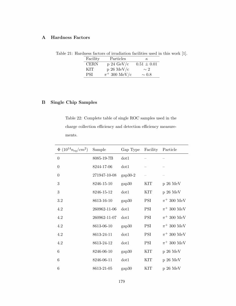
A Hardness Factors
Table 21: Hardness factors of irradiation facilities used in this work [1].Facility Particles κCERN p 24 GeV/c 0.51 ± 0.01KIT p 26 MeV/c ∼ 2PSI π+ 300 MeV/c ∼ 0.8
B Single Chip Samples
Table 22: Complete table of single ROC samples used in the
charge collection efficiency and detection efficiency measure-
ments.
Φ (1014neq/cm2) Sample Gap Type Facility Particle
0 8085-19-7B dot1 – –
0 8244-17-06 dot1 – –
0 271947-10-08 gap30-2 – –
3 8246-15-10 gap30 KIT p 26 MeV
3 8246-15-12 dot1 KIT p 26 MeV
3.2 8613-16-10 gap30 PSI π+ 300 MeV
4.2 260962-11-06 dot1 PSI π+ 300 MeV
4.2 260962-11-07 dot1 PSI π+ 300 MeV
4.2 8613-06-10 gap30 PSI π+ 300 MeV
4.2 8613-24-11 dot1 PSI π+ 300 MeV
4.2 8613-24-12 dot1 PSI π+ 300 MeV
6 8246-06-10 gap30 KIT p 26 MeV
6 8246-06-11 dot1 KIT p 26 MeV
6 8613-21-05 gap30 KIT p 26 MeV
179
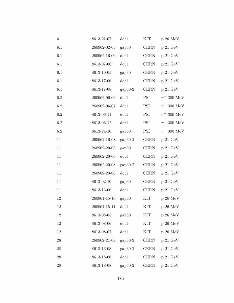
6 8613-21-07 dot1 KIT p 26 MeV
6.1 260962-02-05 gap30 CERN p 21 GeV
6.1 260962-16-06 dot1 CERN p 21 GeV
6.1 8613-07-06 dot1 CERN p 21 GeV
6.1 8613-10-05 gap30 CERN p 21 GeV
6.1 8613-17-06 dot1 CERN p 21 GeV
6.1 8613-17-08 gap30-2 CERN p 21 GeV
6.2 260962-06-06 dot1 PSI π+ 300 MeV
6.2 260962-06-07 dot1 PSI π+ 300 MeV
6.2 8613-06-11 dot1 PSI π+ 300 MeV
6.2 8613-06-12 dot1 PSI π+ 300 MeV
6.2 8613-24-10 gap30 PSI π+ 300 MeV
11 260962-16-08 gap30-2 CERN p 21 GeV
11 260962-20-05 gap30 CERN p 21 GeV
11 260962-20-06 dot1 CERN p 21 GeV
11 260962-20-08 gap30-2 CERN p 21 GeV
11 260962-23-06 dot1 CERN p 21 GeV
11 8613-02-10 gap30 CERN p 21 GeV
11 8613-13-06 dot1 CERN p 21 GeV
12 260961-15-10 gap30 KIT p 26 MeV
12 260961-15-11 dot1 KIT p 26 MeV
12 8613-08-05 gap30 KIT p 26 MeV
12 8613-08-06 dot1 KIT p 26 MeV
12 8613-08-07 dot1 KIT p 26 MeV
28 260962-21-08 gap30-2 CERN p 21 GeV
28 8613-13-08 gap30-2 CERN p 21 GeV
28 8613-18-06 dot1 CERN p 21 GeV
28 8613-18-08 gap30-2 CERN p 21 GeV
180
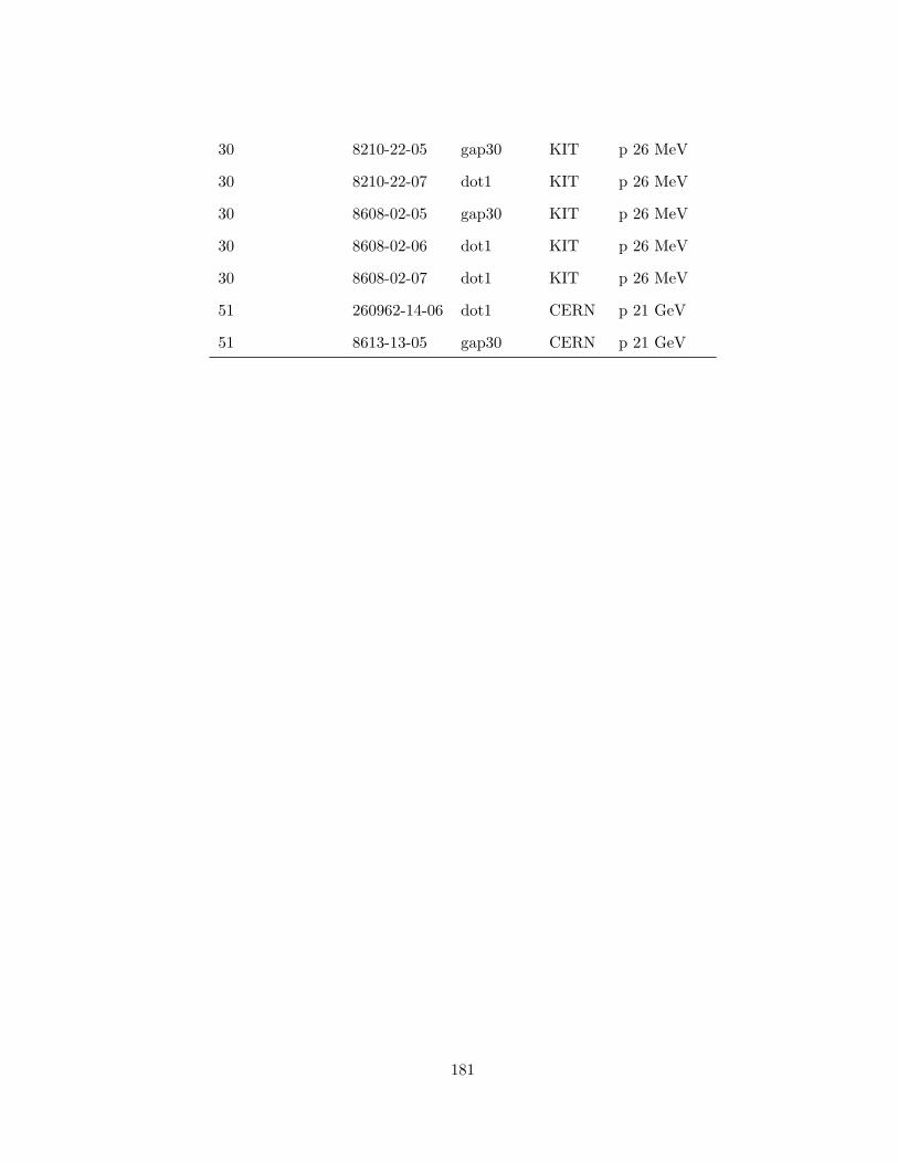
30 8210-22-05 gap30 KIT p 26 MeV
30 8210-22-07 dot1 KIT p 26 MeV
30 8608-02-05 gap30 KIT p 26 MeV
30 8608-02-06 dot1 KIT p 26 MeV
30 8608-02-07 dot1 KIT p 26 MeV
51 260962-14-06 dot1 CERN p 21 GeV
51 8613-13-05 gap30 CERN p 21 GeV
181
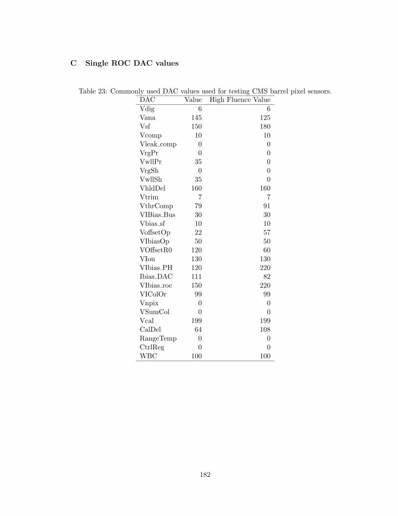
C Single ROC DAC values
Table 23: Commonly used DAC values used for testing CMS barrel pixel sensors.DAC Value High Fluence ValueVdig 6 6Vana 145 125Vsf 150 180Vcomp 10 10Vleak comp 0 0VrgPr 0 0VwllPr 35 0VrgSh 0 0VwllSh 35 0VhldDel 160 160Vtrim 7 7VthrComp 79 91VIBias Bus 30 30Vbias sf 10 10VoffsetOp 22 57VIbiasOp 50 50VOffsetR0 120 60VIon 130 130VIbias PH 120 220Ibias DAC 111 82VIbias roc 150 220VIColOr 99 99Vnpix 0 0VSumCol 0 0Vcal 199 199CalDel 64 108RangeTemp 0 0CtrlReg 0 0WBC 100 100
182

D Backgrounds
D0 invariant mass distribution after each selection cut, showing the signals and the
backgrounds. Classification of backgrounds is shown in Table 24.
Table 24: Background classifications.
Sig Number BG Source-1 Tagging failed1 True signal2 B → τ(τ → µ)D0X3 µ, D0 from different b’s4 µ, D0 from c’s5 µ from light quark6 fake µ7 fake D0
8 both µ, D0 fake9 D0 has more than 2 daughters10 µ, D0 from one b, one c11 K, π switched
183
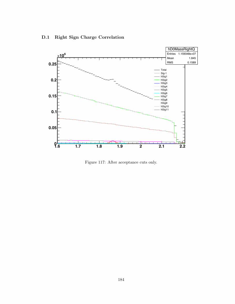
D.1 Right Sign Charge Correlation
hD0MassRightQEntries 1.159348e+07Mean 1.845RMS 0.1589
1.6 1.7 1.8 1.9 2 2.1 2.20
0.05
0.1
0.15
0.2
0.25
610×
hD0MassRightQEntries 1.159348e+07Mean 1.845RMS 0.1589
TotalSig-1hSig1hSig2hSig3hSig4hSig5hSig6hSig7hSig8hSig9hSig10hSig11
Figure 117: After acceptance cuts only.
184
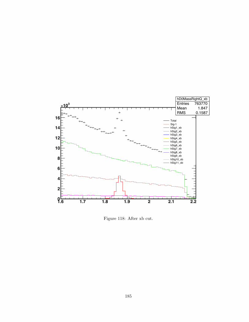
hD0MassRightQ_xbEntries 763770Mean 1.847RMS 0.1587
1.6 1.7 1.8 1.9 2 2.1 2.20
2
4
6
8
10
12
14
16
310×
hD0MassRightQ_xbEntries 763770Mean 1.847RMS 0.1587
TotalSig-1hSig1_xbhSig2_xbhSig3_xbhSig4_xbhSig5_xbhSig6_xbhSig7_xbhSig8_xbhSig9_xbhSig10_xbhSig11_xb
Figure 118: After xb cut.
185

hD0MassRightQ_d0paEntries 146333Mean 1.838RMS 0.1557
1.6 1.7 1.8 1.9 2 2.1 2.20
1
2
3
4
5
310×
hD0MassRightQ_d0paEntries 146333Mean 1.838RMS 0.1557
TotalSig-1hSig1_d0pahSig2_d0pahSig3_d0pahSig4_d0pahSig5_d0pahSig6_d0pahSig7_d0pahSig8_d0pahSig9_d0pahSig10_d0pahSig11_d0pa
Figure 119: After D0 pointing angle cut.
186

hD0MassRightQ_bpaEntries 37078Mean 1.794RMS 0.1315
1.6 1.7 1.8 1.9 2 2.1 2.20
0.5
1
1.5
2
2.5
3
310×
hD0MassRightQ_bpaEntries 37078Mean 1.794RMS 0.1315
TotalSig-1hSig1_bpahSig2_bpahSig3_bpahSig4_bpahSig5_bpahSig6_bpahSig7_bpahSig8_bpahSig9_bpahSig10_bpahSig11_bpa
Figure 120: After B pointing angle cut.
187
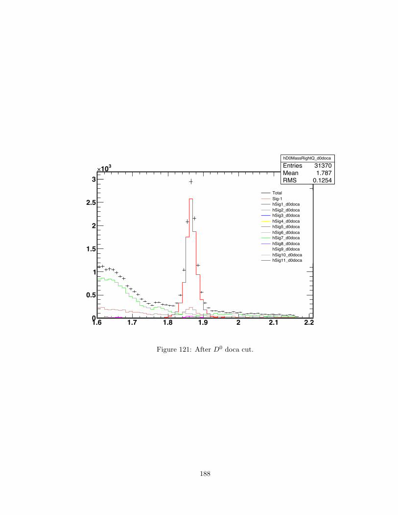
hD0MassRightQ_d0doca
Entries 31370Mean 1.787RMS 0.1254
1.6 1.7 1.8 1.9 2 2.1 2.20
0.5
1
1.5
2
2.5
3
310×
hD0MassRightQ_d0doca
Entries 31370Mean 1.787RMS 0.1254
TotalSig-1hSig1_d0docahSig2_d0docahSig3_d0docahSig4_d0docahSig5_d0docahSig6_d0docahSig7_d0docahSig8_d0docahSig9_d0docahSig10_d0docahSig11_d0doca
Figure 121: After D0 doca cut.
188
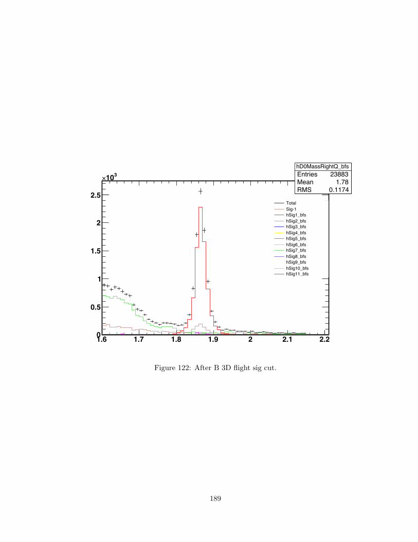
hD0MassRightQ_bfsEntries 23883Mean 1.78RMS 0.1174
1.6 1.7 1.8 1.9 2 2.1 2.20
0.5
1
1.5
2
2.5
310×
hD0MassRightQ_bfsEntries 23883Mean 1.78RMS 0.1174
TotalSig-1hSig1_bfshSig2_bfshSig3_bfshSig4_bfshSig5_bfshSig6_bfshSig7_bfshSig8_bfshSig9_bfshSig10_bfshSig11_bfs
Figure 122: After B 3D flight sig cut.
189

hD0MassRightQ_bdocaEntries 23350Mean 1.779RMS 0.1168
1.6 1.7 1.8 1.9 2 2.1 2.20
0.5
1
1.5
2
2.5
310×
hD0MassRightQ_bdocaEntries 23350Mean 1.779RMS 0.1168
TotalSig-1hSig1_bdocahSig2_bdocahSig3_bdocahSig4_bdocahSig5_bdocahSig6_bdocahSig7_bdocahSig8_bdocahSig9_bdocahSig10_bdocahSig11_bdoca
Figure 123: After B doca cut. (all selection cuts)
190
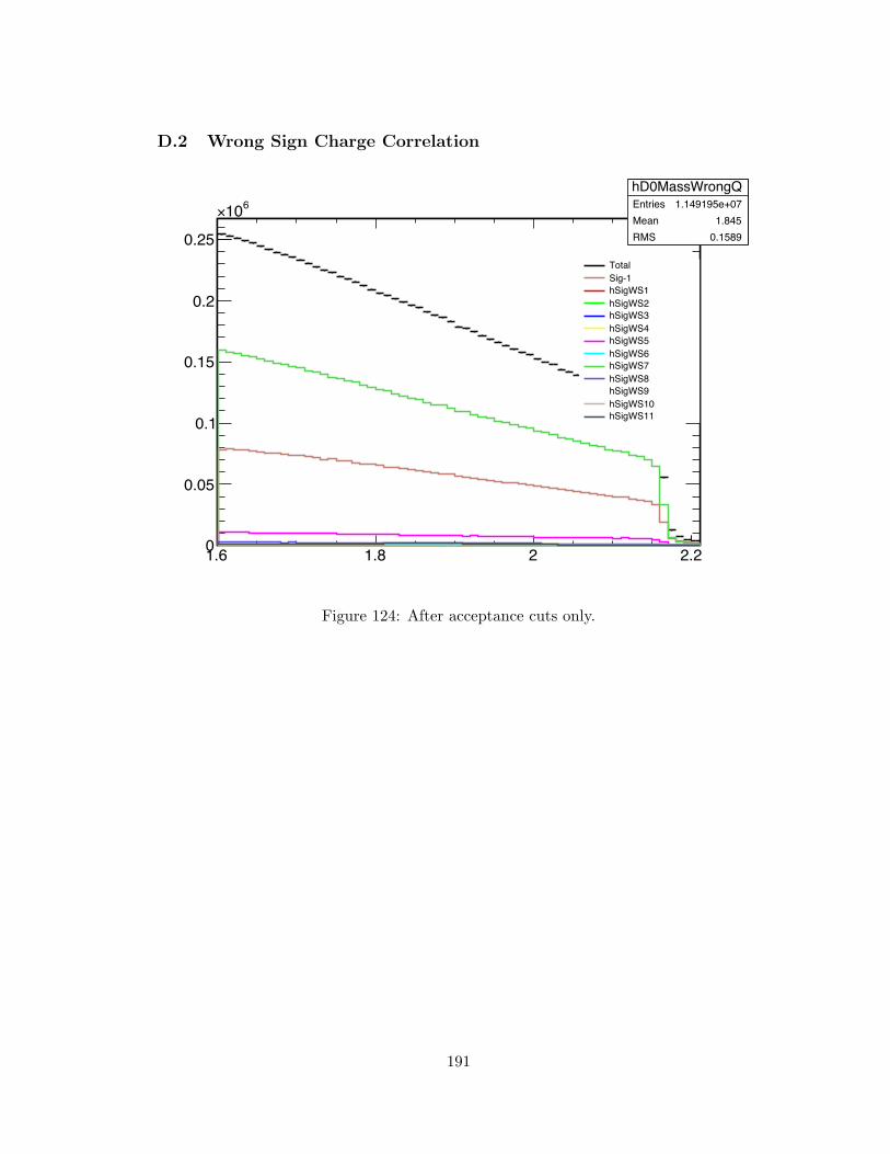
D.2 Wrong Sign Charge Correlation
hD0MassWrongQEntries 1.149195e+07Mean 1.845RMS 0.1589
1.6 1.8 2 2.20
0.05
0.1
0.15
0.2
0.25
610×
hD0MassWrongQEntries 1.149195e+07Mean 1.845RMS 0.1589
TotalSig-1hSigWS1hSigWS2hSigWS3hSigWS4hSigWS5hSigWS6hSigWS7hSigWS8hSigWS9hSigWS10hSigWS11
Figure 124: After acceptance cuts only.
191
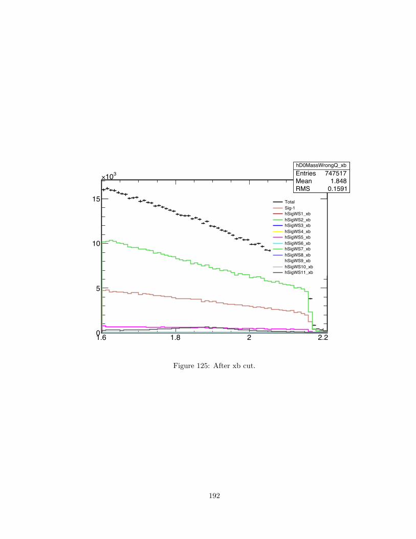
hD0MassWrongQ_xbEntries 747517Mean 1.848RMS 0.1591
1.6 1.8 2 2.20
5
10
15
310×
hD0MassWrongQ_xbEntries 747517Mean 1.848RMS 0.1591
TotalSig-1hSigWS1_xbhSigWS2_xbhSigWS3_xbhSigWS4_xbhSigWS5_xbhSigWS6_xbhSigWS7_xbhSigWS8_xbhSigWS9_xbhSigWS10_xbhSigWS11_xb
Figure 125: After xb cut.
192
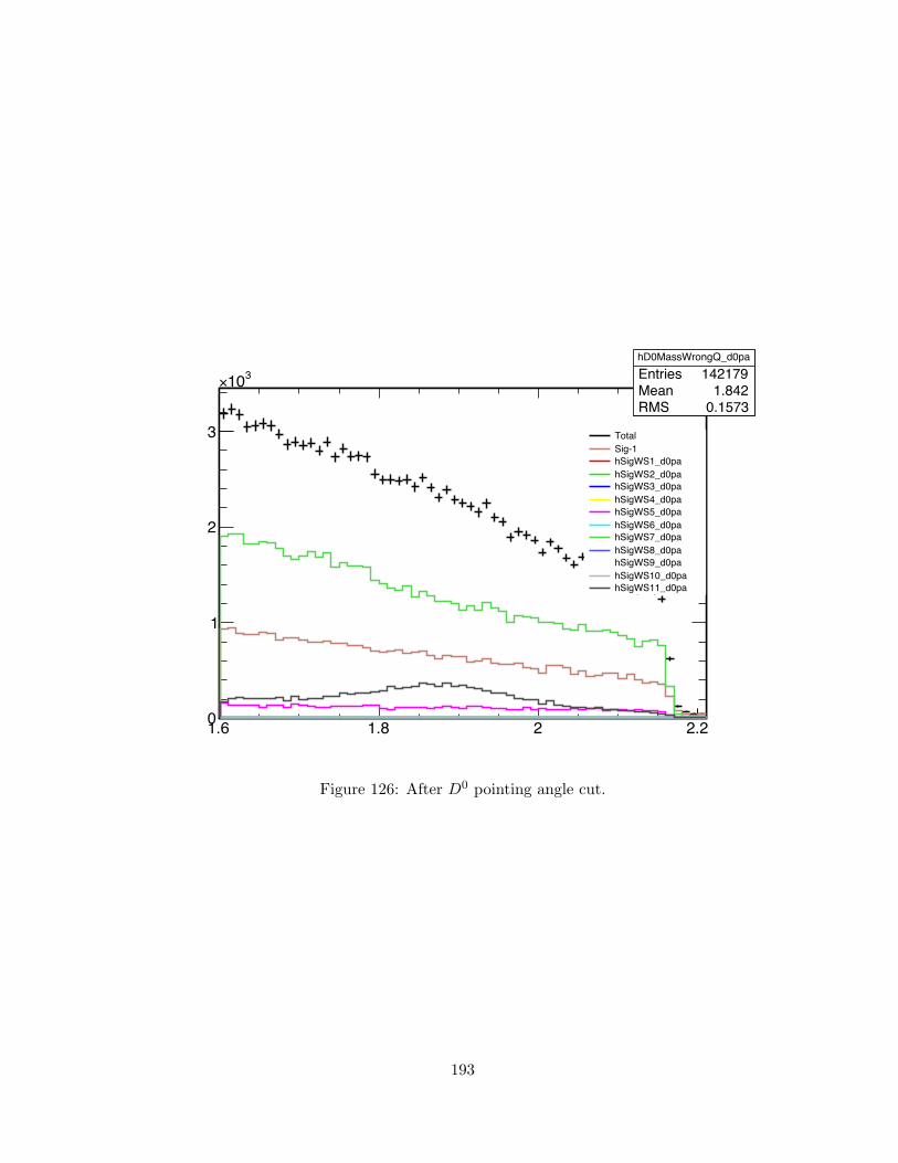
hD0MassWrongQ_d0paEntries 142179Mean 1.842RMS 0.1573
1.6 1.8 2 2.20
1
2
3
310×
hD0MassWrongQ_d0paEntries 142179Mean 1.842RMS 0.1573
TotalSig-1hSigWS1_d0pahSigWS2_d0pahSigWS3_d0pahSigWS4_d0pahSigWS5_d0pahSigWS6_d0pahSigWS7_d0pahSigWS8_d0pahSigWS9_d0pahSigWS10_d0pahSigWS11_d0pa
Figure 126: After D0 pointing angle cut.
193

hD0MassWrongQ_bpaEntries 35147Mean 1.808RMS 0.1434
1.6 1.8 2 2.20
0.2
0.4
0.6
0.8
1
310×
hD0MassWrongQ_bpaEntries 35147Mean 1.808RMS 0.1434
TotalSig-1hSigWS1_bpahSigWS2_bpahSigWS3_bpahSigWS4_bpahSigWS5_bpahSigWS6_bpahSigWS7_bpahSigWS8_bpahSigWS9_bpahSigWS10_bpahSigWS11_bpa
Figure 127: After B pointing angle cut.
194
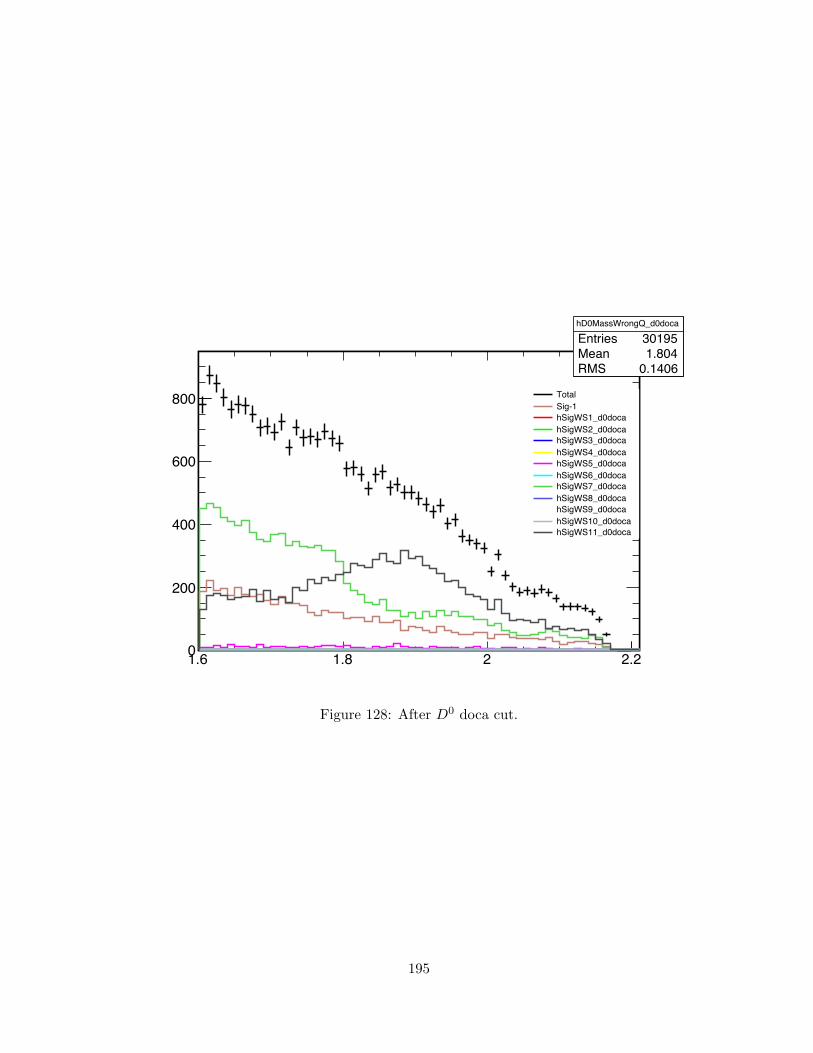
hD0MassWrongQ_d0doca
Entries 30195Mean 1.804RMS 0.1406
1.6 1.8 2 2.20
200
400
600
800
hD0MassWrongQ_d0doca
Entries 30195Mean 1.804RMS 0.1406
TotalSig-1hSigWS1_d0docahSigWS2_d0docahSigWS3_d0docahSigWS4_d0docahSigWS5_d0docahSigWS6_d0docahSigWS7_d0docahSigWS8_d0docahSigWS9_d0docahSigWS10_d0docahSigWS11_d0doca
Figure 128: After D0 doca cut.
195

hD0MassWrongQ_bfsEntries 23434Mean 1.801RMS 0.1379
1.6 1.8 2 2.20
200
400
600
hD0MassWrongQ_bfsEntries 23434Mean 1.801RMS 0.1379
TotalSig-1hSigWS1_bfshSigWS2_bfshSigWS3_bfshSigWS4_bfshSigWS5_bfshSigWS6_bfshSigWS7_bfshSigWS8_bfshSigWS9_bfshSigWS10_bfshSigWS11_bfs
Figure 129: After B 3D flight sig cut.
196
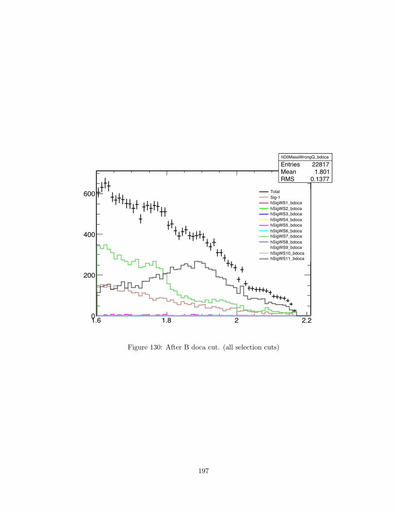
hD0MassWrongQ_bdoca
Entries 22817Mean 1.801RMS 0.1377
1.6 1.8 2 2.20
200
400
600
hD0MassWrongQ_bdoca
Entries 22817Mean 1.801RMS 0.1377
TotalSig-1hSigWS1_bdocahSigWS2_bdocahSigWS3_bdocahSigWS4_bdocahSigWS5_bdocahSigWS6_bdocahSigWS7_bdocahSigWS8_bdocahSigWS9_bdocahSigWS10_bdocahSigWS11_bdoca
Figure 130: After B doca cut. (all selection cuts)
197

E Alternate Cut Optimization
In order to show that the order chosen for the cut variables does not change the end re-
sult, the cut optimization was redone. The variable with the second highest significance
was chosen as the first variable in the procedure. The xb variable is deliberately chosen
last to ensure that it does not influence the choice of cut value on the other variables.
The distributions for the first pass are shown again in Figure 131.
(a) µ signed transverse impact pa-rameter
hpasssigEntries 100Mean 0.05088RMS 0.02814
0 0.02 0.04 0.06 0.08 0.10
0.5
1
1.5
hpasssigEntries 100Mean 0.05088RMS 0.02814
D0 doca (cm)
(b) D0 doca
(c) B doca
hpasssigEntries 100Mean 0.5239RMS 0.2641
0 0.2 0.4 0.6 0.8 1
0.5
1
1.5
2
2.5
hpasssigEntries 100Mean 0.5239RMS 0.2641
xb
(d) xb
Figure 131: Distributions of S/√B after the quality cuts.
From these distributions we see that the B doca variable has the second best sig-
nificance after the acceptance and quality cuts, and the significance is maximum at a
cut value of 0.007. For the second pass, we require B doca < 0.007 and repeat the
procedure for all other variables. The distributions for the second pass are shown in
Figure 132.
After the second pass we determine that the D0 doca shows the best significance
aside from the xb variable. The maximum is at a cut value of 0.015. For the third
pass, we repeat the procedure, requiring that both B doca > 0.007 and the D0 doca
198

(a) µ signed transverse impact pa-rameter
hpasssigEntries 100Mean 0.05122RMS 0.02807
0 0.02 0.04 0.06 0.08 0.10
0.5
1
1.5
2
hpasssigEntries 100Mean 0.05122RMS 0.02807
(b) D0 doca
hpasssigEntries 100Mean 0.5229RMS 0.264
0 0.2 0.4 0.6 0. 1
1
2
3
hpasssigEntries 100Mean 0.5229RMS 0.264
(c) sb
Figure 132: Distributions of S/√B after the quality cuts, and B doca > 0.007.
< 0.015. The distributions for the remaining variables after the third pass are shown in
Figure 133.
Because the muon transverse impact parameter does not show any significant dis-
crimination between signal and background except in the right tail of the distribution,
this variable is not used. The maximum value of the significance of the xb variable is at
0.7. Finally, for the event selection we require:
1. The B doca is less than 0.007.
2. The D0 doca is less than 0.015.
3. xb is greater than 0.7.
Changing the order of the variable selection resulted in the same final cut selection.
Therefore the cuts are considered to be stable and unbiased.
199

(a) µ signed transverse impact parameter
hpasssigEntries 100Mean 0.525RMS 0.2648
0 0.2 0.4 0.6 0.8 1
1
2
3
hpasssigEntries 100Mean 0.525RMS 0.2648
(b) xb
Figure 133: Distributions of S/√B after the acceptance cuts, B > 0.007, and D0 doca
< 0.015.
200
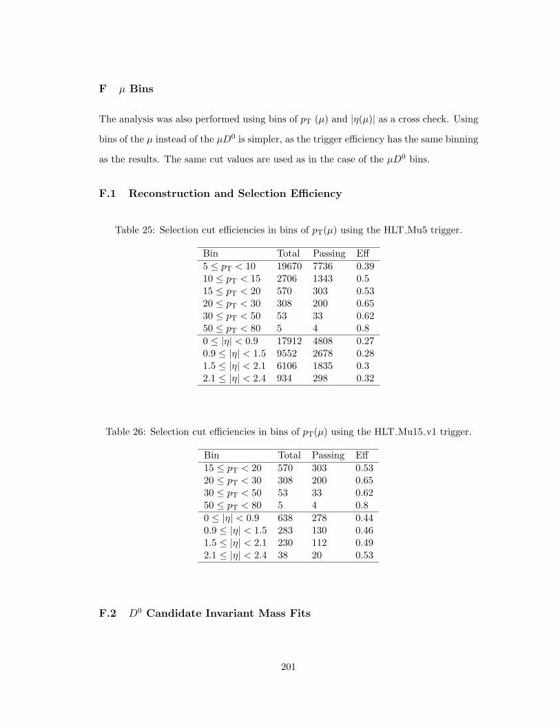
F µ Bins
The analysis was also performed using bins of pT (µ) and |η(µ)| as a cross check. Using
bins of the µ instead of the µD0 is simpler, as the trigger efficiency has the same binning
as the results. The same cut values are used as in the case of the µD0 bins.
F.1 Reconstruction and Selection Efficiency
Table 25: Selection cut efficiencies in bins of pT(µ) using the HLT Mu5 trigger.
Bin Total Passing Eff5 ≤ pT < 10 19670 7736 0.3910 ≤ pT < 15 2706 1343 0.515 ≤ pT < 20 570 303 0.5320 ≤ pT < 30 308 200 0.6530 ≤ pT < 50 53 33 0.6250 ≤ pT < 80 5 4 0.80 ≤ |η| < 0.9 17912 4808 0.270.9 ≤ |η| < 1.5 9552 2678 0.281.5 ≤ |η| < 2.1 6106 1835 0.32.1 ≤ |η| < 2.4 934 298 0.32
Table 26: Selection cut efficiencies in bins of pT(µ) using the HLT Mu15 v1 trigger.
Bin Total Passing Eff15 ≤ pT < 20 570 303 0.5320 ≤ pT < 30 308 200 0.6530 ≤ pT < 50 53 33 0.6250 ≤ pT < 80 5 4 0.80 ≤ |η| < 0.9 638 278 0.440.9 ≤ |η| < 1.5 283 130 0.461.5 ≤ |η| < 2.1 230 112 0.492.1 ≤ |η| < 2.4 38 20 0.53
F.2 D0 Candidate Invariant Mass Fits
201
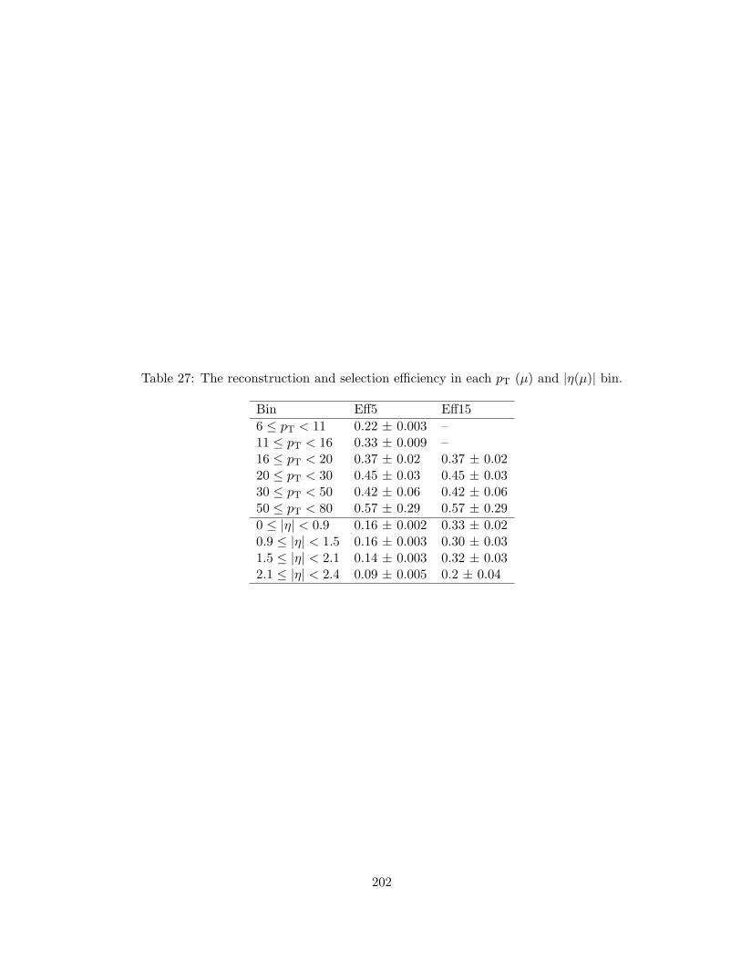
Table 27: The reconstruction and selection efficiency in each pT (µ) and |η(µ)| bin.
Bin Eff5 Eff156 ≤ pT < 11 0.22 ± 0.003 –11 ≤ pT < 16 0.33 ± 0.009 –16 ≤ pT < 20 0.37 ± 0.02 0.37 ± 0.0220 ≤ pT < 30 0.45 ± 0.03 0.45 ± 0.0330 ≤ pT < 50 0.42 ± 0.06 0.42 ± 0.0650 ≤ pT < 80 0.57 ± 0.29 0.57 ± 0.290 ≤ |η| < 0.9 0.16 ± 0.002 0.33 ± 0.020.9 ≤ |η| < 1.5 0.16 ± 0.003 0.30 ± 0.031.5 ≤ |η| < 2.1 0.14 ± 0.003 0.32 ± 0.032.1 ≤ |η| < 2.4 0.09 ± 0.005 0.2 ± 0.04
202

(GeV)πKm1.75 1.8 1.85 1.9 1.95 2
entri
es
0
0.5
1
1.5
2
2.5
310×
hacD0MassRightQ_pt5Entries 24689Mean 1.861RMS 0.04284
/ ndf 2χ 33.74 / 19Prob 0.01972p0 66.0± 1543 p1 34.3± -742.7 p2 0.000± 1.866 p3 98.0± 713.5 p4 67.8± 1623 p5 0.0000± 0.0065 p6 0.00033± 0.01564
(a) 5 ≤ pT < 10
(GeV)πKm1.75 1.8 1.85 1.9 1.95 2
entri
es
0
100
200
300
400
hacD0MassRightQ_pt10Entries 4592Mean 1.862RMS 0.04316
/ ndf 2χ 38 / 19Prob 0.005943p0 26.9± 224.3 p1 14.0± -106.1 p2 0.000± 1.865 p3 43.8± 68.8 p4 32.6± 320.4 p5 0.0000± 0.0065 p6 0.00074± 0.01491
(b) 10 ≤ pT < 15
(GeV)πKm1.75 1.8 1.85 1.9 1.95 2
entri
es
0
20
40
60
80
100
hacD0MassRightQ_pt15Entries 1068Mean 1.861RMS 0.04173
/ ndf 2χ 19.57 / 18Prob 0.3576p0 13.74± 59.94 p1 7.19± -28.96 p2 0.001± 1.864 p3 24.31± 23.71 p4 18.71± 71.65 p5 0.0000± 0.0065 p6 0.00192± 0.01469
(c) 15 ≤ pT < 20
(GeV)πKm1.75 1.8 1.85 1.9 1.95 2
entri
es
0
20
40
60
80
hacD0MassRightQ_pt20Entries 728Mean 1.863RMS 0.04422
/ ndf 2χ 24.61 / 19Prob 0.1739p0 9.80± 15.37 p1 5.136± -6.568 p2 0.001± 1.866 p3 11.54± 43.91 p4 5.84± 28.26 p5 0.0000± 0.0065 p6 0.00245± 0.02097
(d) 20 ≤ pT < 30
(GeV)πKm1.75 1.8 1.85 1.9 1.95 2
entri
es
0
5
10
15
hacD0MassRightQ_pt30Entries 135Mean 1.851RMS 0.03634
/ ndf 2χ 4.617 / 8Prob 0.7976p0 14.95± 13.38 p1 8.094± -6.453 p2 0.003± 1.864 p3 7.920e+00± 3.933e-10 p4 2.6± 10.2 p5 0.0000± 0.0065 p6 0.00231± 0.01131
(e) 30 ≤ pT < 50
Figure 134: D0 mass distributions in bins of pT (GeV/c) for Monte Carlo events.
203

(GeV)πKm1.75 1.8 1.85 1.9 1.95 2
entri
es
0
200
400
600
hacD0MassRightQ_abseta0Entries 4937Mean 1.861RMS 0.0403
/ ndf 2χ 51.34 / 20Prob 0.000142p0 27.2± 250.5 p1 14.2± -121.3 p2 0.000± 1.865 p3 98.01± 68.61 p4 84.7± 590.3 p5 0.0000± 0.0065 p6 0.0005± 0.0104
(a) 0.0 ≤ |η| < 0.3
(GeV)πKm1.75 1.8 1.85 1.9 1.95 2
entri
es
0
0.2
0.4
0.6
0.8
1
1.2
310×hacD0MassRightQ_abseta1
Entries 10440Mean 1.862RMS 0.04037
/ ndf 2χ 50.04 / 20Prob 0.0002185p0 39.4± 523.6 p1 20.6± -250.9 p2 0.000± 1.865 p3 86.4± 269.7 p4 67.0± 889.3 p5 0.0000± 0.0065 p6 0.00041± 0.01297
(b) 0.3 ≤ |η| < 0.9
(GeV)πKm1.75 1.8 1.85 1.9 1.95 2
entri
es
0
200
400
600
hacD0MassRightQ_abseta2Entries 9023Mean 1.861RMS 0.04495
/ ndf 2χ 34.53 / 20Prob 0.02275p0 42.0± 596.4 p1 21.8± -287.6 p2 0.000± 1.865 p3 47.7± 116.9 p4 32.2± 544.5 p5 0.0000± 0.0065 p6 0.00058± 0.01753
(c) 0.9 ≤ |η| < 1.5
(GeV)πKm1.75 1.8 1.85 1.9 1.95 2
entri
es
0
100
200
300
400
hacD0MassRightQ_abseta3Entries 5920Mean 1.861RMS 0.04527
/ ndf 2χ 13.3 / 20Prob 0.8643p0 34.8± 370.5 p1 18.0± -177.9 p2 0.000± 1.865 p3 29.58± 67.61 p4 17.3± 292.7 p5 0.0000± 0.0065 p6 0.00086± 0.02239
(d) 1.5 ≤ |η| < 2.1
(GeV)πKm1.75 1.8 1.85 1.9 1.95 2
entri
es
0
20
40
60
hacD0MassRightQ_abseta4Entries 908Mean 1.865RMS 0.04659
/ ndf 2χ 43.04 / 20Prob 0.00202p0 12.91± 46.54 p1 6.69± -22.18 p2 0.000± 1.865 p3 8.070e+00± 8.244e-09 p4 4.38± 48.36 p5 0.0000± 0.0065 p6 0.00176± 0.02162
(e) 2.1 ≤ |η| < 2.4
Figure 135: D0 mass distributions in bins of |η| for Monte Carlo events.
204

(GeV)πKm1.75 1.8 1.85 1.9 1.95 2
entri
es
0
10
20
30
40
50
hacD0MassRightQ_abseta0Entries 324Mean 1.86RMS 0.04528
/ ndf 2χ 17.67 / 20Prob 0.6091p0 7.17± 20.54 p1 3.745± -9.766 p2 0.000± 1.865 p3 5.253e+01± 5.584e-09 p4 5.50± 42.35 p5 0.0000± 0.0065 p6 0.000853± 0.009554
(a) 0.0 ≤ |η| < 0.3
(GeV)πKm1.75 1.8 1.85 1.9 1.95 2
entri
es
0
20
40
60
80
100
120
140hacD0MassRightQ_abseta1
Entries 1014Mean 1.862RMS 0.04232
/ ndf 2χ 21.78 / 20Prob 0.3528p0 12.32± 48.57 p1 6.45± -22.94 p2 0.000± 1.865 p3 28.9± 41.8 p4 22.7± 77.2 p5 0.0000± 0.0065 p6 0.00132± 0.01203
(b) 0.3 ≤ |η| < 0.9
(GeV)πKm1.75 1.8 1.85 1.9 1.95 2
entri
es
0
10
20
30
40
50
hacD0MassRightQ_abseta2Entries 524Mean 1.856RMS 0.04205
/ ndf 2χ 17.15 / 20Prob 0.6433p0 11.89± 42.51 p1 6.02± -21.16 p2 0.000± 1.865 p3 8.61± 28.71 p4 3.90± 14.59 p5 0.0000± 0.0065 p6 0.00672± 0.02743
(c) 0.9 ≤ |η| < 1.5
(GeV)πKm1.75 1.8 1.85 1.9 1.95 2
entri
es
0
5
10
15
20
25
hacD0MassRightQ_abseta3Entries 356Mean 1.863RMS 0.04416
/ ndf 2χ 24.79 / 20Prob 0.2097p0 7.12± 12.35 p1 3.717± -5.733 p2 0.000± 1.865 p3 2.304e+00± 1.409e-11 p4 2.45± 19.82 p5 0.0000± 0.0065 p6 0.00210± 0.02355
(d) 1.5 ≤ |η| < 2.1
(GeV)πKm1.75 1.8 1.85 1.9 1.95 2
entri
es
0
2
4
6
8
hacD0MassRightQ_abseta4Entries 53Mean 1.869RMS 0.03091
/ ndf 2χ 17.26 / 20Prob 0.6361p0 2.679± -5.441 p1 1.368± 2.833 p2 0.000± 1.865 p3 8.876e-01± 4.926e-07 p4 0.953± 4.084 p5 0.0000± 0.0065 p6 0.0047± 0.0267
(e) 2.1 ≤ |η| < 2.4
Figure 136: D0 mass distributions in bins of |η| for Monte Carlo events with pT (µ) >15GeV.
205
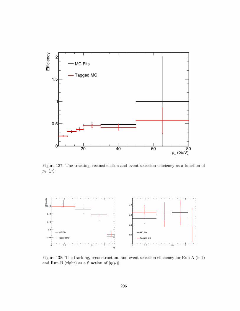
(GeV)T
p20 40 60 80
Effic
ienc
y
0
0.5
1
1.5
2MC Fits
Tagged MC
Figure 137: The tracking, reconstruction and event selection efficiency as a function ofpT (µ).
|η|0 0.5 1 1.5 2
Effic
ienc
y
0.08
0.1
0.12
0.14
0.16
MC Fits
Tagged MC
0 0.5 1 1.5 2
0.1
0.2
0.3
0.4
MC Fits
Tagged MC
Figure 138: The tracking, reconstruction, and event selection efficiency for Run A (left)and Run B (right) as a function of |η(µ)|.
206

(GeV)πKm1.75 1.8 1.85 1.9 1.95 2
entri
es
0
50
100
150
200
hacD0MassRightQ_pt5Entries 1932Mean 1.859RMS 0.04768
/ ndf 2χ 33.92 / 19Prob 0.01881p0 23.0± 146.3 p1 11.93± -70.96 p2 0.001± 1.863 p3 24.80± 72.28 p4 15.64± 99.45 p5 0.0000± 0.0065 p6 0.00169± 0.01849
(a) 5 ≤ pT < 10
(GeV)πKm1.75 1.8 1.85 1.9 1.95 2
entri
es
0
10
20
30
40
hacD0MassRightQ_pt10Entries 411Mean 1.864RMS 0.04976
/ ndf 2χ 20.41 / 20Prob 0.4324p0 9.11± 10.14 p1 4.8± -3.9 p2 3.35± 28.69 p3 0.000± 1.865 p4 0.000± 0.015
(b) 10 ≤ pT < 15
(GeV)πKm1.75 1.8 1.85 1.9 1.95 2
entri
es
0
5
10
15
hacD0MassRightQ_pt15Entries 90Mean 1.863RMS 0.04936
/ ndf 2χ 9.49 / 11Prob 0.5768p0 10.593± 5.493 p1 5.634± -2.105 p2 0.00± 1.86 p3 1.235e+01± 1.073e-10 p4 2.484± 7.391 p5 0.0000± 0.0065 p6 0.00286± 0.01096
(c) 15 ≤ pT < 20
(GeV)πKm1.75 1.8 1.85 1.9 1.95 2
entri
es
0
2
4
6
8
10
hacD0MassRightQ_pt20Entries 56Mean 1.858RMS 0.03993
/ ndf 2χ 5.332 / 8Prob 0.7216p0 0.544± 1.074 p1 0.2935± 0.2326 p2 0.012± 1.855 p3 7.77± 2.93 p4 57.968± 2.852 p5 0.0000± 0.0065 p6 0.345± 0.001
(d) 20 ≤ pT < 30
Figure 139: D0 mass distributions in bins of pT (GeV/c) for the 2010A dataset.
207
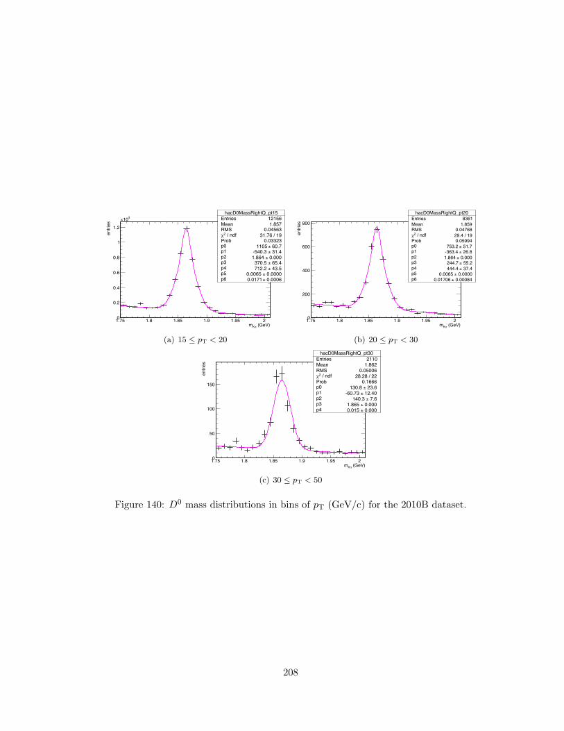
(GeV)πKm1.75 1.8 1.85 1.9 1.95 2
entri
es
0
0.2
0.4
0.6
0.8
1
1.2
310×
hacD0MassRightQ_pt15Entries 12156Mean 1.857RMS 0.04563
/ ndf 2χ 31.76 / 19Prob 0.03323p0 60.7± 1105 p1 31.4± -540.3 p2 0.000± 1.864 p3 65.4± 370.5 p4 43.5± 712.2 p5 0.0000± 0.0065 p6 0.0006± 0.0171
(a) 15 ≤ pT < 20
(GeV)πKm1.75 1.8 1.85 1.9 1.95 2
entri
es
0
200
400
600
800
hacD0MassRightQ_pt20Entries 8361Mean 1.859RMS 0.04768
/ ndf 2χ 29.4 / 19Prob 0.05994p0 51.7± 753.2 p1 26.8± -363.4 p2 0.000± 1.864 p3 55.2± 244.7 p4 37.4± 444.4 p5 0.0000± 0.0065 p6 0.00084± 0.01706
(b) 20 ≤ pT < 30
(GeV)πKm1.75 1.8 1.85 1.9 1.95 2
entri
es
0
50
100
150
hacD0MassRightQ_pt30Entries 2110Mean 1.862RMS 0.05006
/ ndf 2χ 28.28 / 22Prob 0.1666p0 23.6± 130.8 p1 12.40± -60.73 p2 7.6± 140.3 p3 0.000± 1.865 p4 0.000± 0.015
(c) 30 ≤ pT < 50
Figure 140: D0 mass distributions in bins of pT (GeV/c) for the 2010B dataset.
208
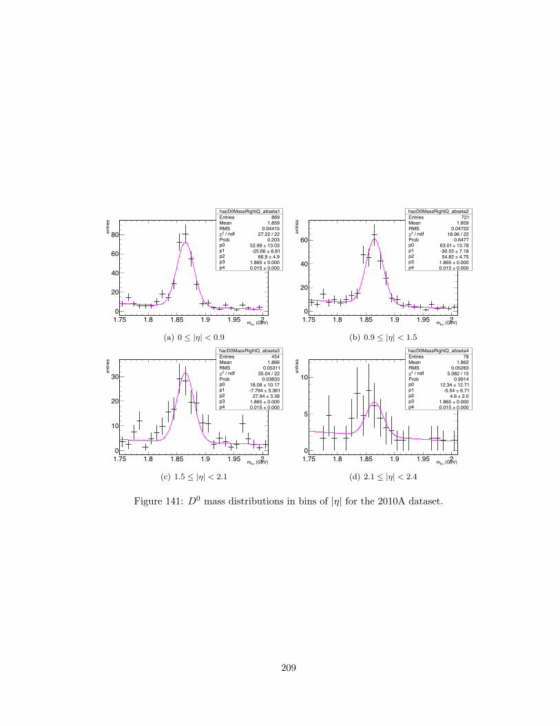
(GeV)πKm1.75 1.8 1.85 1.9 1.95 2
entri
es
0
20
40
60
80
hacD0MassRightQ_abseta1Entries 869Mean 1.859RMS 0.04415
/ ndf 2χ 27.22 / 22Prob 0.203p0 13.03± 52.99 p1 6.81± -25.66 p2 4.9± 66.9 p3 0.000± 1.865 p4 0.000± 0.015
(a) 0 ≤ |η| < 0.9
(GeV)πKm1.75 1.8 1.85 1.9 1.95 2
entri
es
0
20
40
60
hacD0MassRightQ_abseta2Entries 721Mean 1.859RMS 0.04722
/ ndf 2χ 18.96 / 22Prob 0.6477p0 13.78± 63.01 p1 7.18± -30.55 p2 4.75± 54.82 p3 0.000± 1.865 p4 0.000± 0.015
(b) 0.9 ≤ |η| < 1.5
(GeV)πKm1.75 1.8 1.85 1.9 1.95 2
entri
es
0
10
20
30
hacD0MassRightQ_abseta3Entries 454Mean 1.866RMS 0.05311
/ ndf 2χ 35.04 / 22Prob 0.03833p0 10.17± 18.08 p1 5.361± -7.794 p2 3.39± 27.94 p3 0.000± 1.865 p4 0.000± 0.015
(c) 1.5 ≤ |η| < 2.1
(GeV)πKm1.75 1.8 1.85 1.9 1.95 2
entri
es
0
5
10
hacD0MassRightQ_abseta4Entries 78Mean 1.862RMS 0.05283
/ ndf 2χ 5.082 / 15Prob 0.9914p0 12.71± 12.34 p1 6.71± -5.54 p2 2.0± 4.6 p3 0.000± 1.865 p4 0.000± 0.015
(d) 2.1 ≤ |η| < 2.4
Figure 141: D0 mass distributions in bins of |η| for the 2010A dataset.
209
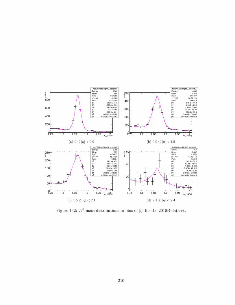
(GeV)πKm1.75 1.8 1.85 1.9 1.95 2
entri
es
0
200
400
600
800
hacD0MassRightQ_abseta1Entries 8362Mean 1.858RMS 0.04356
/ ndf 2χ 44 / 20Prob 0.001505p0 41.3± 662.6 p1 21.4± -325.5 p2 0.000± 1.865 p3 69.5± 237 p4 51.4± 607.9 p5 0.0000± 0.0065 p6 0.00052± 0.01382
(a) 0 ≤ |η| < 0.9
(GeV)πKm1.75 1.8 1.85 1.9 1.95 2
entri
es
0
100
200
300
400
500hacD0MassRightQ_abseta2
Entries 6330Mean 1.859RMS 0.04877
/ ndf 2χ 30.32 / 20Prob 0.06478p0 44.4± 516.3 p1 23.1± -246.8 p2 0.000± 1.865 p3 38.24± 39.56 p4 24.3± 356.3 p5 0.0000± 0.0065 p6 0.00078± 0.01932
(b) 0.9 ≤ |η| < 1.5
(GeV)πKm1.75 1.8 1.85 1.9 1.95 2
entri
es
0
50
100
150
200
250
hacD0MassRightQ_abseta3Entries 3786Mean 1.859RMS 0.04937
/ ndf 2χ 16.5 / 20Prob 0.6854p0 37.2± 346.9 p1 19.2± -167.4 p2 0.000± 1.865 p3 23.57± 21.34 p4 13.5± 178.9 p5 0.0000± 0.0065 p6 0.00133± 0.02464
(c) 1.5 ≤ |η| < 2.1
(GeV)πKm1.75 1.8 1.85 1.9 1.95 2
entri
es
0
20
40
60hacD0MassRightQ_abseta4
Entries 347Mean 1.852RMS 0.0571
/ ndf 2χ 17.42 / 19Prob 0.5618p0 30.2± 102.2 p1 15.60± -49.83 p2 0.000± 1.865 p3 12.513± 6.979 p4 6.84± 16.75 p5 0.0000± 0.0065 p6 0.00813± 0.02594
(d) 2.1 ≤ |η| < 2.4
Figure 142: D0 mass distributions in bins of |η| for the 2010B dataset.
210

F.3 Wrong Charge Correlation Distributions
(GeV)πKm1.75 1.8 1.85 1.9 1.95 2
entri
es
20
40
60
80
hacD0MassWrongQEntries 2473Mean 1.859RMS 0.07064
/ ndf 2χ 27.24 / 27Prob 0.4509p0 15.0± 207.6 p1 6.6± -185.3 p2 15.0± 189 p3 0.000e+00± 0 p4 0.0± inf
(GeV)πKm1.75 1.8 1.85 1.9 1.95 2
entri
es
200
300
400
500
600
700
hacD0MassWrongQEntries 25007Mean 1.858RMS 0.07198
/ ndf 2χ 46.38 / 27Prob 0.01156p0 33.7± 1330 p1 40.4± -1551 p2 47.0± 2030 p3 0.000e+00± 0 p4 0.0± inf
(GeV)πKm1.75 1.8 1.85 1.9 1.95 2
entri
es
200
300
400
500
600
700
hacD0MassWrongQEntries 31271Mean 1.861RMS 0.07207
/ ndf 2χ 68.74 / 27Prob 1.693e-05p0 46.2± 1411 p1 20.4± -1686 p2 46.3± 2253 p3 0.000e+00± 0 p4 0.0± inf
Figure 143: D0 mass distribution of the wrong charge correlation candidates for thewhole pT and η range for the 2010A data (top left), 2010B data (top right), and MonteCarlo events (bottom).
F.4 Systematic Uncertainties
The systematic uncertainty due to the trigger efficiency is found by varying the trigger
efficiency up and down, and checking the effect on the final cross section in each bin.
The uncertainty for each bin resulting from the error on the trigger efficiency is shown
in Tables 28.
The systematic uncertainty due to the selection efficiency is found by varying the
selection efficiency by the error on the efficiency. This is the dominant uncertainty in
this analysis, due to the low statistics in the Monte Carlo. The uncertainty for each bin
resulting from the error on the selection efficiency is shown in Tables 30 and 31.
As in the case of using bins of the µD0, the total bin-independent systematic uncer-
211
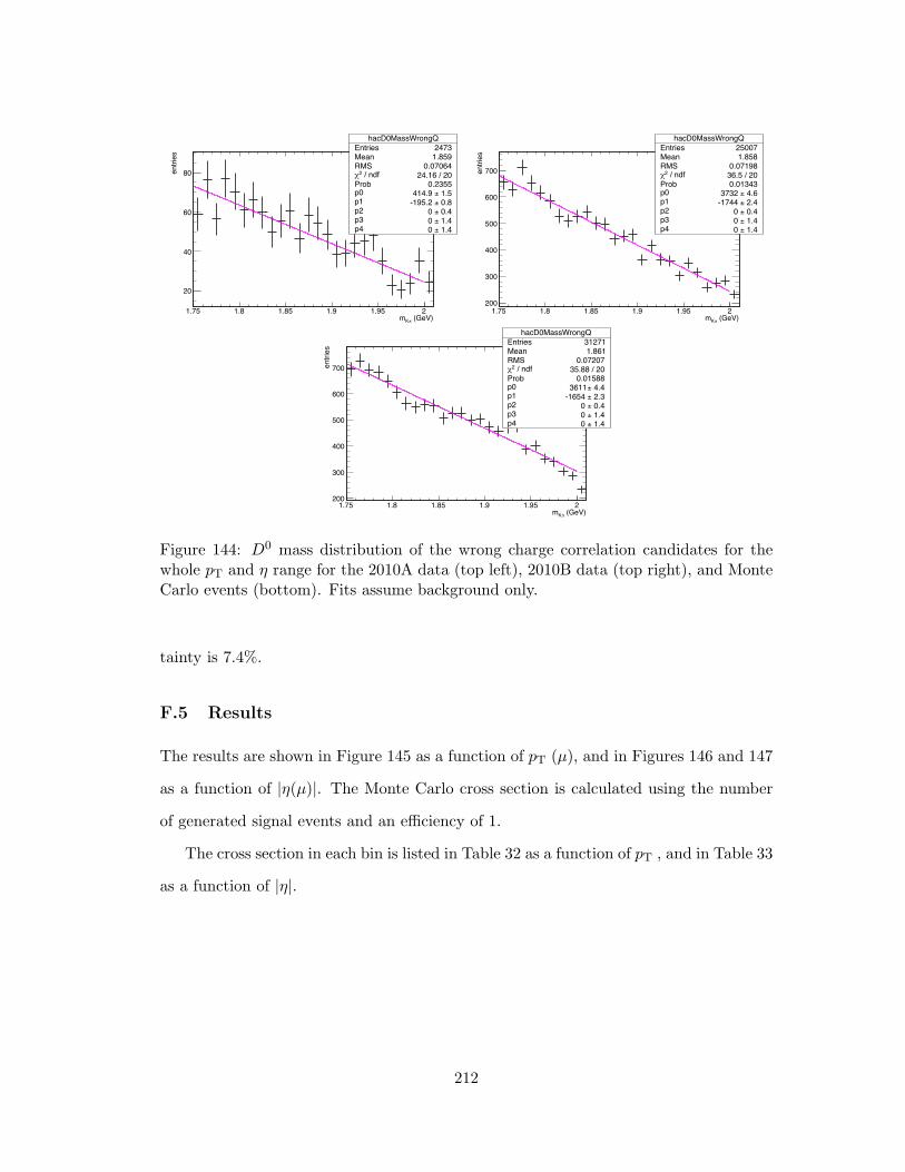
(GeV)πKm1.75 1.8 1.85 1.9 1.95 2
entri
es
20
40
60
80
hacD0MassWrongQEntries 2473Mean 1.859RMS 0.07064
/ ndf 2χ 24.16 / 20Prob 0.2355p0 1.5± 414.9 p1 0.8± -195.2 p2 0.4± 0 p3 1.4± 0 p4 1.4± 0
(GeV)πKm1.75 1.8 1.85 1.9 1.95 2
entri
es
200
300
400
500
600
700
hacD0MassWrongQEntries 25007Mean 1.858RMS 0.07198
/ ndf 2χ 36.5 / 20Prob 0.01343p0 4.6± 3732 p1 2.4± -1744 p2 0.4± 0 p3 1.4± 0 p4 1.4± 0
(GeV)πKm1.75 1.8 1.85 1.9 1.95 2
entri
es
200
300
400
500
600
700
hacD0MassWrongQEntries 31271Mean 1.861RMS 0.07207
/ ndf 2χ 35.88 / 20Prob 0.01588p0 4.4± 3611 p1 2.3± -1654 p2 0.4± 0 p3 1.4± 0 p4 1.4± 0
Figure 144: D0 mass distribution of the wrong charge correlation candidates for thewhole pT and η range for the 2010A data (top left), 2010B data (top right), and MonteCarlo events (bottom). Fits assume background only.
tainty is 7.4%.
F.5 Results
The results are shown in Figure 145 as a function of pT (µ), and in Figures 146 and 147
as a function of |η(µ)|. The Monte Carlo cross section is calculated using the number
of generated signal events and an efficiency of 1.
The cross section in each bin is listed in Table 32 as a function of pT , and in Table 33
as a function of |η|.
212

(GeV/c) T
p0 10 20 30 40 50
(nb/
GeV
)T
X’)
/ dp
0 Dµ
→ b
+X
→(p
p σd -210
-110
1
10
210
310
Run ARun BMC
Run ARun BMC
= 7 TeV sCMS,
)| < 2.4µ(η|
Figure 145: Cross section as a function of pT(µ) for Run A (black), Run B (blue), andMonte Carlo (red) events. Error bars show the statistical uncertainty, and the coloredbands show the combined statistical and systematic uncertainty.
| η|0 0.5 1 1.5 2 2.5
| (nb
)η
X’)
/ d|
0 Dµ
→ b
+X
→(p
p σd
0
1
2
3
4
5
6310×
Run AMCRun AMC
= 7 TeV sCMS,
) > 6 GeV/cµ(Tp
Figure 146: Cross section as a function of |η|(µ) for Run A (black) and Monte Carlo(red) events. Error bars show the statistical uncertainty, and the colored band showsthe combined statistical and systematic uncertainty.
213
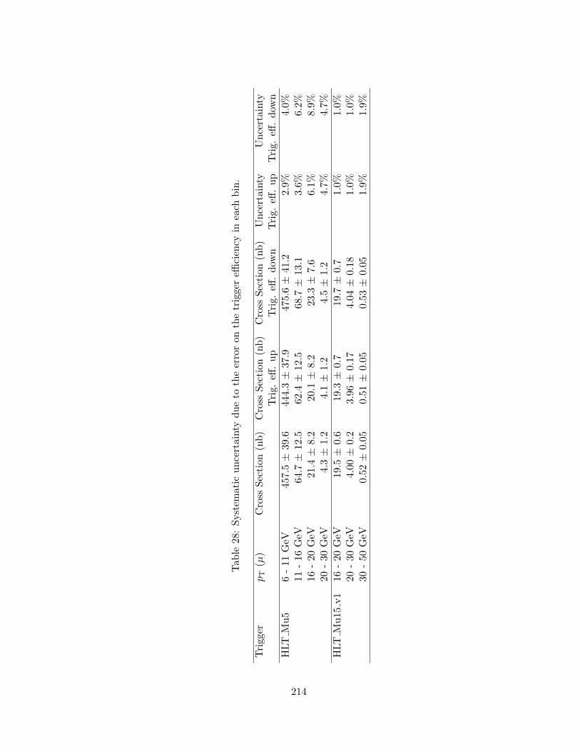
Tab
le28
:Systematic
uncertaintydueto
theerroron
thetriggereffi
ciency
ineach
bin.
Trigg
erp T
(µ)
Cross
Section
(nb)
Cross
Section
(nb)
Cross
Section
(nb)
Uncertainty
Uncertainty
Trig.
eff.up
Trig.
eff.dow
nTrig.
eff.up
Trig.
eff.dow
nHLT
Mu5
6-11
GeV
457.5±
39.6
444.3±
37.9
475.6±
41.2
2.9%
4.0%
11-16
GeV
64.7
±12
.562
.4±
12.5
68.7
±13
.13.6%
6.2%
16-20
GeV
21.4
±8.2
20.1
±8.2
23.3
±7.6
6.1%
8.9%
20-30
GeV
4.3±
1.2
4.1±
1.2
4.5±
1.2
4.7%
4.7%
HLT
Mu15
v116
-20
GeV
19.5
±0.6
19.3
±0.7
19.7
±0.7
1.0%
1.0%
20-30
GeV
4.00
±0.2
3.96
±0.17
4.04
±0.18
1.0%
1.0%
30-50
GeV
0.52
±0.05
0.51
±0.05
0.53
±0.05
1.9%
1.9%
214
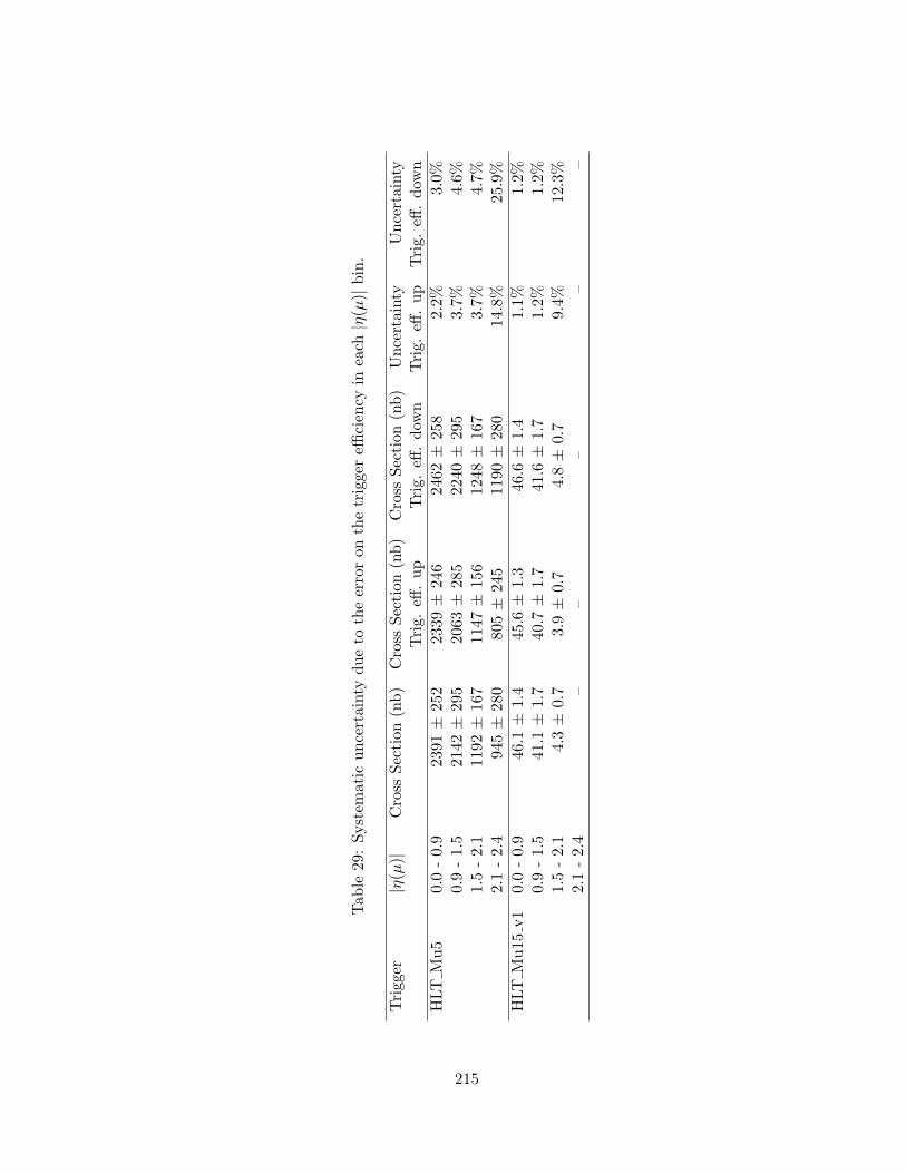
Tab
le29
:Systematic
uncertaintydueto
theerroron
thetriggereffi
ciency
ineach
|η(µ)|
bin.
Trigg
er|η(µ)|
Cross
Section
(nb)
Cross
Section
(nb)
Cross
Section
(nb)
Uncertainty
Uncertainty
Trig.
eff.up
Trig.
eff.dow
nTrig.
eff.up
Trig.
eff.dow
nHLT
Mu5
0.0-0.9
2391
±25
223
39±
246
2462
±25
82.2%
3.0%
0.9-1.5
2142
±29
520
63±
285
2240
±29
53.7%
4.6%
1.5-2.1
1192
±16
711
47±
156
1248
±16
73.7%
4.7%
2.1-2.4
945±
280
805±
245
1190
±28
014
.8%
25.9%
HLT
Mu15
v10.0-0.9
46.1
±1.4
45.6
±1.3
46.6
±1.4
1.1%
1.2%
0.9-1.5
41.1
±1.7
40.7
±1.7
41.6
±1.7
1.2%
1.2%
1.5-2.1
4.3±
0.7
3.9±
0.7
4.8±
0.7
9.4%
12.3%
2.1-2.4
––
––
–
215
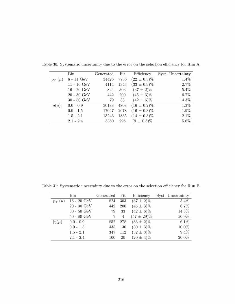
Table 30: Systematic uncertainty due to the error on the selection efficiency for Run A.
Bin Generated Fit Efficiency Syst. UncertaintypT (µ) 6 - 11 GeV 34426 7736 (22 ± 0.3)% 1.4%
11 - 16 GeV 4114 1343 (33 ± 0.9)% 2.7%16 - 20 GeV 824 303 (37 ± 2)% 5.4%20 - 30 GeV 442 200 (45 ± 3)% 6.7%30 - 50 GeV 79 33 (42 ± 6)% 14.3%
|η(µ)| 0.0 - 0.9 30188 4808 (16 ± 0.2)% 1.3%0.9 - 1.5 17047 2678 (16 ± 0.3)% 1.9%1.5 - 2.1 13243 1835 (14 ± 0.3)% 2.1%2.1 - 2.4 3380 298 (9 ± 0.5)% 5.6%
Table 31: Systematic uncertainty due to the error on the selection efficiency for Run B.
Bin Generated Fit Efficiency Syst. UncertaintypT (µ) 16 - 20 GeV 824 303 (37 ± 2)% 5.4%
20 - 30 GeV 442 200 (45 ± 3)% 6.7%30 - 50 GeV 79 33 (42 ± 6)% 14.3%50 - 80 GeV 7 4 (57 ± 29)% 50.9%
|η(µ)| 0.0 - 0.9 852 278 (33 ± 2)% 6.1%0.9 - 1.5 435 130 (30 ± 3)% 10.0%1.5 - 2.1 347 112 (32 ± 3)% 9.4%2.1 - 2.4 100 20 (20 ± 4)% 20.0%
216

| η|0 0.5 1 1.5 2 2.5
| (nb
)η
X’)
/ d|
0 Dµ
→ b
+X
→(p
p σd
0
50
100
150
Run BMCRun BMC
= 7 TeV sCMS,
) > 16 GeV/cµ(Tp
Figure 147: Cross section as a function of |η|(µ) for Run B (blue) and Monte Carlo(red) events. Error bars show the statistical uncertainty, and the colored band showsthe combined statistical and systematic uncertainty.
217
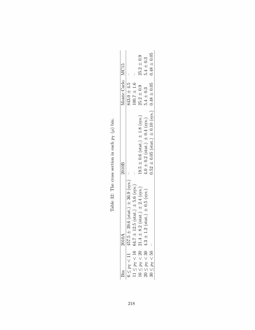
Tab
le32
:Thecrosssectionin
each
p T(µ)bin.
Bin
2010A
2010B
Mon
teCarlo
MC15
6≤
p T<
1145
7.5±
39.6
(stat.)±
36.9
(sys.)
–84
3.0±
4.5
–11
≤p T
<16
64.7
±12
.5(stat.)±
5.6(sys.)
–10
0.7±
1.6
–16
≤p T
<20
21.4
±8.2(stat.)±
2.4(sys.)
19.5
±0.6(stat.)±
1.8(sys.)
25.2
±0.9
25.2
±0.9
20≤
p T<
304.3±
1.2(stat.)±
0.5(sys.)
4.0±
0.2(stat.)±
0.4(sys.)
5.4±
0.3
5.4±
0.3
30≤
p T<
50–
0.52
±0.05
(stat.)±
0.10
(sys.)
0.48
±0.05
0.48
±0.05
218

Tab
le33
:Thecrosssectionin
each
|η(µ)|
bin.
Bin
2010
A20
10B
Mon
teCarlo
MC15
0≤
|η|<
0.9
1595
.9±
607.3(stat.)±
125.1(sys.)
1699.1
±13
3.9(stat.)±
162.8(sys.)
4106
.9±
23.6
4106
.9±
94.6
0.9≤
|η|<
1.5
2161
.6±
510.9(stat.)±
183.6(sys.)
1966.4
±16
5.2(stat.)±
292.1(sys.)
3478
.8±
26.6
3478
.8±
229.6
1.5≤
|η|<
2.1
1347
.9±
356.5(stat.)±
114.2(sys.)
200.1±
138.1(stat.)±
24.2
(sys.)
2702
.5±
23.5
2702
.5±
163.7
2.1≤
|η|<
2.4
1225
.5±
770.3(stat.)±
239.3(sys.)
–13
79.5
±23
.713
79.5
±12
2.6
219


