Application of Copulas to Estimation of Joint Crop Yield Distributions
Dmitry Vedenov
Department of Agricultural Economics
Texas A&M University 2124 TAMU
College Station, TX 77843‐2124 E‐mail: [email protected]
Tel: 979‐845‐8491 Selected Paper prepared for presentation at the American Agricultural Economics
Association Annual Meeting, Orlando, FL, July 2729, 2008. This paper reports results of research in progress. Updated versions of the paper
may be available in the future. Contact the author before quoting. © Copyright 2008 by Dmitry Vedenov. All rights reserved. Readers may make verbatim copies of this document for noncommercial purposes by any means, provided that this copyright notice appears on all such copies.

2
Introduction
Correct estimation of crop yield distribution is commonly acknowledged to be of
paramount importance in analysis of issues in crop insurance and risk management (Ker
and Coble, 2003). Estimation of single yield distributions has received considerable
attention in recent years. Sherrick, et al. (2004) compare performance of alternative
parametric distributions in modeling farm level yields for Illinois farms. Ramirez, Misra and
Field (2003) suggest a family of parametric distributions that allows for nonnormality of
yields. Goodwin and Ker (1998) and Ker and Goodwin (2000) discuss (nonparametric)
kernel density approach to yield modeling, which allows for more flexibility than
parametric distributions. Ker and Coble (2003) introduce a semi‐parametric estimator that
combines benefits of both parametric and non‐parametric estimators. All authors, however,
acknow s. ledge a common problem of short data series, especially for the farm‐level yield
While a single yield distribution suffices in many applications (e.g. determining
premiums and optimal coverage levels for yield insurance), many applied problems call for
joint distributions of various yields. For example, if a producer grows corn and soybeans on
the same farm, the full‐farm risk management problem requires knowledge of a joint yield
distribution of the two crops. Similarly, a joint distribution of farm‐level and county‐level
yields is necessary in order to find an optimal coverage level for an area‐yield contract (e.g.
Group Risk Plan) under general assumptions on producer’s risk preferences.
Unfortunately, modeling of joint yield distributions based on historical data is
affected by shortness of data series even more severely than in a univariate case. Indeed,
the same limited number of observations has to provide information both on the
distributions of individual yields and the dependence structure between them. To a large
3
procedures involve transform
extent, the existing literature tries to circumvent the problem rather than tackling it
directly. Commonly used approaches include using mean‐variance criterion or assuming
regressibility of the random variables modeled.
The mean‐variance criterion does not require the knowledge of the full distribution
and only depends on its first two moments easily estimated from historical data. However,
the ranking of random alternatives based on this criterion is known to be consistent with
the expected utility maximization only when the underlying distributions satisfy location
and scale condition (Meyer, 1987), which is rarely the case with yield distributions.
Regressibility assumption essentially states that, in case of two1 random variables,
one variable can be completely described as a linear function of the other plus an
uncorrelated random shock (see, for example, Hau, 1999). The linear coefficient is typically
known as beta (e.g. Miranda, 1991) and is proportional to the correlation between the
variables. Thus the regressibility assumption essentially states that the dependence
between the random variables of interest is completely captured by the linear correlation.
However, the latter is known to be a poor measure of dependence, as is commonly
illustrated by the example of a standard normal variable and its square. Furthermore, if the
uncorrelated random shocks are assumed normal, regressibility amounts to joint
multivariate normality — an assumption crop yields typically violate (Ramirez, Misra and
Field, 2003; Sherrick, et al., 2004).
Many papers recognize the limitations of the above approaches and employ various
ad hoc procedures to model the dependence between the yields. Most of the time, these
ations of multivariate normal distribution with the
1 The following arguments can be extended to a multivariate case as well.

4
parameters estimated from data (Ramirez, 1997; Coble, Heifner and Zuniga, 2000). While
this approach allows greater flexibility in modeling joint distributions, it still implicitly
relies on the assumption that the correlation matrix contains all necessary information
about the dependence structure.
A multivariate empirical distribution is probably the closest to preserving the
information contained in the data without imposing distributional assumptions (Deng,
Barnett and Vedenov, 2007). However, the empirical distributions are limited to the
observed realizations and results in discontinuous density functions, which is particularly
problematic in evaluating expected losses and payoffs of insurance contracts.
Copulas provide an alternative way to model joint distributions of random variables
with greater flexibility both in terms of marginal distributions and the dependence
structure. Copulas have been used in financial literature for quite sometime (see, for
example, Cherubini, Luciano and Vecchiato, 2004; Chen and Huang, 2007; Fernandez,
2008), but have not made their way yet to the agricultural economics literature. The
purpose of the present paper is to demonstrate the application of copulas to modeling of
joint yield distributions, analyze relative performance of different modeling assumptions,
and illustrate the effect of different modeling methodology on a typical risk management
problem of selecting optimal coverage for an area‐yield insurance contract.
The rest of the paper is organized as follows. The next section presents a brief
theory behind the copulas and outlines the procedure of modeling joint distributions using
copulas. The following section illustrates the methodology by estimating the joint
distribution of farm‐ and county‐yield for Iowa corn and evaluates its performance relative
to alternative modeling approaches. The last section presents concluding remarks.

Copulas and Joint Distributions
Overvie
5
)0,(
w of Copulas
A two‐dimensional copula is defined as a function),( vuC 2 ]1,0[]1,0[: 2 →C with the
following properties:
0),0( == vuC C all , for ]1,0[∈vu
nd
auuC =)1,( vvC =),1( for al l ]1, 0[, ∈vu
0),(),(),(),( 11211222 ≥+−− vuCvuCvuCvuC for all 2121 , vvuu ≤≤ .
Copulas are related to joint bivariate distributions by virtu of Sklar’s Theorem (Nelsen,
2006, p. 15), which states that any distribution function
e
),( yxH with margins ) and (xF
)( yG can be represented as
))(),((),( yGxFCyxH = , (1)
where ),( ⋅⋅C is a uniquely d termined copula function. The theorem also states that any two
distribution functions )(xF and )(
e
yG combined with an arbitrary copula C according to (1)
result in a joint distribution function ( y with the margins F and G. ),xHC
If the distribution functions and the copula in (1) are continuous, Sklar’s theorem
can be restated in terms of the probability densities as
)()())(),((),( ygxfyGxFcyxh ⋅⋅= , (1’)
where yx
h∂∂
, , yxHyx
∂=
),(),(2
)(')( xFxf = )(')( yGyg = , and vu
c∂∂
is the copula
d to as the canonical representation essentially decomposes
vuCvu =
),(),(2
density. Eq. (1’) often referre
∂
2 The following is a brief summary of theory behind the copulas limited to two‐dimensional copulas for brevity sake. A more formal and thorough presentation on the topic can be found in Nelsen, 2006.
the joint distribution of two variables into a product of marginal densities and the
dependence structure captured by the copula density (Cherubini, Luciano and Vecchiato,
2004).
From the practical standpoint, (1’) allows both derivation of copulas from a known
distribution and construction of a joint distribution given marginal distributions and the
copula. For example, if h is a bivariate standard normal distribution with the correlation ρ
and the standard normal margins, then (1’) implies the Gaussian copula density
6
⎟⎟⎠⎝ −− )1(221 2 ρρ
where Φ(·) is the cumulative density function of the standard normal distribution. The
Gaussian copula is parameterized by a single parameter, which can be estimated from the
historic
⎞⎜⎜⎛ ΦΦ−ΦΦ
+ΦΦ
=−−−−− ))(())(()()(2))(())((exp1),( 2
2121112121 vuvuvuvuc , (2) −+ −ρ
al data in a straightforward fashion.
The real advantage of copulas, however, comes from the fact that once the copula is
derived or estimated, it can be applied to any pair of marginal distributions, not necessarily
those implied by the original joint distribution. For instance, the Gaussian density (2) can
be combined in (1’) with a beta distribution f and a Student distribution g to result in a joint
density function h, which is neither bivariate normal, nor beta, nor Student. This property
is particularly useful in modeling yield distributions, as it allows one to estimate marginal
yield densities either parametrically or nonparametrically (e.g. by one of the methods
mentioned in the Introduction) and then combine them into a joint distribution using a
selected copula function.
For all its flexibility, the copula approach has one serious shortcoming. Generally
speaking, there are an infinite number of copula functions and any one can be used in (1’)
to combine margins into a joint distribution. In a sense, this means substituting one
arbitrary choice (that of a parametric distributional form) by another (that of a copula
function). Several parametric copulas have been frequently used in financial literature
including the Gaussian copula in (2) as well as Student, Frank, and Gumbel copulas
(Cherubini, Luciano and Vecchiato, 2004). Relative performance of different copulas can be
measured against each other, but there is no constructive way to determine the “optimal”
copula function (Kole, Koedijk and Verbeek, 2007).
An alternative approach is to use a nonparametric copula estimated from the
available data. This is similar to using nonparametric techniques such as empirical
distribution and kernel density estimation in a univariate case. In particular, a kernel
copula can be estimated based on a multivariate analog of kernel density estimator as
outlined below.
7
n
Kernel Copula
A kernel copula can be constructed from (1’) by setting h equal to the kernel density
estimate of the joint distribution, and f and g to the kernel density estimates of the
corresponding marginals. A general form kernel density estimator of a univariate
probability density function f can be writte as
∑ ⎟=
⎞⎜⎛ −
=n
iXxKxf ),(ˆ τ
⎠⎝in 1 ττ
where niiX 1}{ = are observations (i.i.d. draws from the distribution being estimated), K(∙) is a
kernel function, and τ is a smoothing parameter called bandwidth.
1 , (3)
3
3 The theory behind the kernel density estimator and the choice of the kernel function and bandwidth is beyond the scope of the present paper. A more detailed exposition can be found in (Wand and Jones, 1995).

A bivariate analog of (3) can be written as
8
∑ ⎟⎟=
⎞⎜⎜⎛ −−
=n
ii YyXxKyxh 21 ,),,,(ˆ ττ
o
⎠⎝in 1 2121 ττττ
where all the notation corresponds to (3), except that the kernel function now has two
arguments and different smoothing parameters can be used along each dimension. There
are several options for choosing the bivariate kernel function, but the most straightforward
way is to use the product of two univariate (although not necessarily the same) kernels
(Wand
1 , (4)
and Jones, 1995).
Based on (1’), (3), and (4), the verall procedure for estimating the kernel copula
from a series o 4f historical data iii YX 1},{ = can be outlined as follows.
Step 1. Construct the kernel density estimates of marginal distributions f and g
accordin
n
g to (3) using appropriate kernels Kj and bandwidths τj.
Step 2. Calculate the cumulative density functions corresponding to f and g (e.g. by
numerical integration)
∫∑∞
⎟⎟⎞
⎜⎜⎛ −
=n
i dX
KxF 1)(ˆ ξξ
− = ⎠⎝in 1 11 ττ
x1 and ∫∑∞ =
⎟⎟⎞
⎜⎜⎛ −
=y n
i dY
Ky 21)(ˆ η
η
− ⎠⎝in 1 22 ττ
Step 3. Construct kernel density estimate of the joint density h according to (4)
using the product kernel and the same bandwidths as in Step 1.
G (5)
Step 4. Estimate the copula density at any given point (u,v) based on (1’), namely
))(ˆ(ˆ))(ˆ(ˆ))(ˆ),(ˆ(ˆ),(ˆ
11
11
vGguFf
vGuFhvuc
−−
−−
⋅= , (6)
4 Note that in the rest of the section the dependence of the estimated kernel density functions on the bandwidth is suppressed for brevity sake.
where )(ˆ 1 uF − and )(ˆ 1 vG − are inverse functions to the cumulative densities
estimated in (5), which can be obtained by solving numerically the root‐finding
problems uxF =)( and vyG =)( for given u and v, respectively.
Just as in the case of Gaussian copula mentioned above, once estimated, the kernel copula
can be combined with any estimates of the marginal distributions of f and g, either
parametric or nonparametric.
ˆ ˆ
MonteCarlo Simulations
Many problems in crop insurance and risk management require calculating a
criterion defined as a function of random variables. For example, the expected utility
framework calls for maximization of the expected utility of a revenue or profit function,
which is expressed in terms of realizations of one or more random variables. While the
expectation can be computed using the joint density function estimated according to (1’),
the process involves numerical integration and thus requires calculation of the estimated
copula
9
draw from a copula C, then
and margins at a large number of integration nodes.5
Monte‐Carlo method is often more computationally efficient in solving these
problems, in particular when the number of random variables is large (Miranda and
Fackler, 2002). Sklar’s Theorem (1) provides a constructive way to generate Monte‐Carlo
draws from the joint distribution implied by a copula C and margins F and G. The method is
based on the fact that any copula function by itself is a joint distribution of random
variables with uniform margins on [0,1] (Nelsen, 2006). In particular, if },{ vu is a random
is a random draw from the joint )}(),({},{ 11 vGuFyx −−=
5 The direct integration approach suffers from so‐called curse of dimensionality in the sense that the number of integration nodes increases exponentially in the number of random variables.

distribution ))(),((),( yGxFCyxH = . In turn, random draws from a given copulas can be
generated by using the conditional sampling method (see, for example, Cherubini, Luciano
and Vecchiato, 2004, p. 182).
In the two‐dimensional case, the overall algorithm of generating Monte‐Carlo draws
from the joint . distribution of variables of interest can be outlined as follows
Step 1. Select or estimate a copula function C and marginal densities F and G.
Step 2. Generate a necessary number of draws from two independent
uniform
Nj 1},{ =ηξ
distributions on [0,1].
Step 3. Use the first series as is, i.e. set jju ζ= for all j = 1,...,N, and calculate the
distributions of v conditional on realization of uj as
10
juuu =∂
Step 4. Transform each draw j
jj
CuvC =)|( . ∂
η using the corresponding inverse conditional
distribution function (conditional copula) to obtain the second series of draws, i.e.
set )| for all j = 1,..., N. ( jjj
Step 5. Transform the generated pairs using the inverse margins, i.e. set
)}),{ −=
1j uCv η−=
Njjj vu 1},{ =
((},{ jjjj vGuFyx
For parametric copulas, the conditional copulas can be usually calculated analytically either
from the copula function itself or from the copula density. In case of the kernel copula, a
numerical integration of copula density in (6) can be used.
11 − for all j = 1,...,N.

11
Application
Data
The application of copula methodology is illustrated by modeling a joint distribution
of county‐ and farm‐level yields. Such distributions are of interest, for example, when
evaluating risk‐reducing effectiveness of area‐yield contracts such as GRP. A common
problem with estimating farm‐level yield distributions is that the available data series are
typically very short (6‐10 years). Therefore, any estimation of a joint distribution or a
dependence structure between county‐level yields and individual farm yields are
extremely unreliable. A representative farmer approach is typically used instead, where all
available farm‐level data within a given county are pooled together and treated as draws
from a distribution of farm yields within the county (Schnitkey, Sherrick and Irwin, 2003;
Deng, Barnett and Vedenov, 2007). For the purposes of this analysis, a farm‐level data for
corn yields in Kossuth County, IA, are used. 6 The data set includes observations for 90
farms over the period between 1980 and 1994, with at least 12 years worth of yields
available for each farm.
County‐level yield series are typically much longer and are available from the
National Agricultural Statistical Service (USDA/NASS, 2008). County yield series from 1967
to 2007 were detrended using a simple log‐linear trend and adjusted to their 2007
equivalents (Vedenov and Barnett, 2004). Given shortness of farm‐level yield series, the
estimated county trend was used to detrend those as well. The detrended farm‐level yields
for each year were also adjusted to ensure that their average is equal to the detrended
6 Results for other crops and/or regions may be available in the future.

12
county yield for that year.7
The sample statistics of detrended farm‐ and county‐level yields are presented in
Table 1. Both farm and county yields are skewed to the left and leptokurtic, suggesting
nonnormality. As expected, farm‐level yields exhibit greater variability and range than the
county‐level yields.
[Table 1 about here]
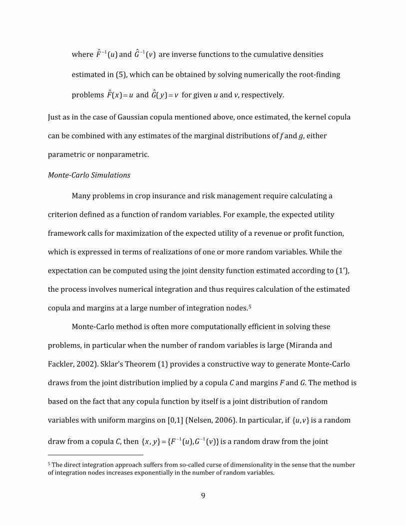
The scatter‐plot of detrended farm‐level yields versus the corresponding county
yields is shown in Figure 1. One conclusion that can be made from the figure is that the
farm‐level yields exhibit different variability for different realizations of county yields,
suggesting that assuming joint normality, or regressing farm yields on county yields may
produce misleading results. Therefore, modeling the full joint distribution is of particular
importance in this situation.
[Figure 1 about here]
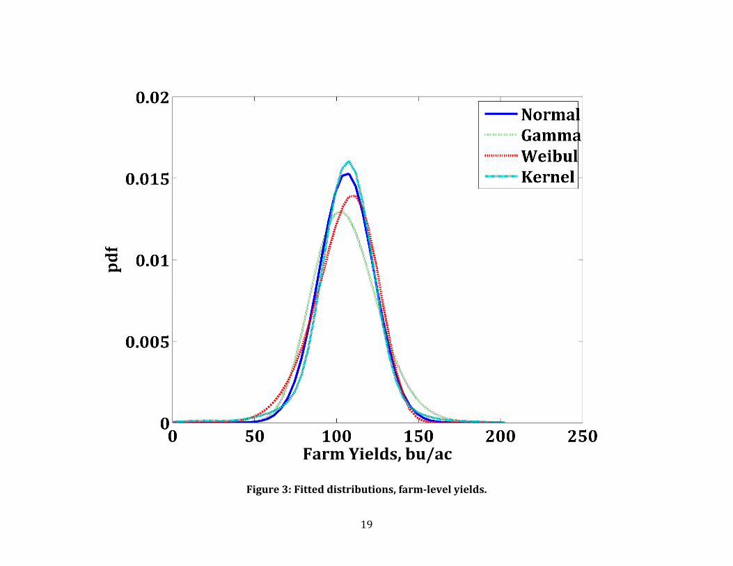
Gaussian copula (2) and kernel copula (6) were used to model the dependence
structure between the county and farm yields. The dataset included 1,137 pairs of
county/farm yield observation, which were used to estimate the parameters of Gaussian
copula and the density of kernel copula. In order to illustrate the flexibility of copula
approach, four distributions frequently used in the literature — normal, gamma, Weibul,
and nonparametric kernel density — were fitted to the data to model marginal
distributions of county and farm level yields.
7 This adjustment is necessary to reflect the fact that the farms included in the sample may not necessarily represent all possible yields in the county.
13
In particular, county yield margins were estimated using the entire series from 1967
to 2007, while all available 1,137 farm yield observations were used to fit the farm‐level
yield densities. The fitted marginal n in Figures 2 and 3. distributions are show
[Figure 2 about here]
[Figure 3 about here]
The joint distributions of county and farm‐level yields were then estimated using the Sklar
theorem. The combination of four marginal distributions and two copulas resulted in eight
joint distributions.8 The contours of the estimated distributions superimposed on the
scatter‐plots of original data are shown in Figure 4 for Gaussian copula and in Figure 5 for
kernel copula.
[Figure 4 about here]
[Figure 5 about here]
Note that the normal margins combined with Gaussian copula result in a bivariate
normal distribution, while kernel copula combined with kernel density margins result in a
bivariate kernel density estimate of the joint distribution. However, one of the advantages
of copula approach is that the copula and the margins do not have to be estimated from the
same samples. This property is particularly useful in the example presented here, since the
farm‐level yields only match to a small portion of county‐yield series. While matching
observations are used to estimate the copula, longer county yield series are used to
estimate their marginal distribution.
8 The same types of marginal distributions were used for both farm and county yields in each case. However copula approach can easily accommodate margins of different type.
14
In order to evaluate how well the estimated joint distributions reflect the historical
data, the log‐likelihood criterion was calculated in each case. The results are summarized in
Table 2.
[Table 2 about here]
The results in figures 4 and 5 illustrate the importance of selecting both the correct copula
and the marginal distributions. Gaussian copula tends to generate elliptic distributions
regardless of the margins, which may lead to underestimating the dependence away from
the mean. Given that analysis of risk management and insurance typically concerns with
tail events, Gaussian copula may not be the best choice. In terms of goodness‐of‐fit as
measured by the log‐likelihood of the estimated joint distributions, a combination of
Gaussian copula and kernel density margins provides the best fit of the data followed by
Weibul and normal margins. All parametric margins seem to have problems with fitting the
outlying series of observations corresponding to the Midwest flood of 1993.
Distributions based on kernel copula seem to do much better job reflecting the
shape of the original data than those based on Gaussian copula. However, the failure of
parametric margins to capture the very same set of outlying observation resulted in log‐
likelihood criterion equal to negative infinity for joint distributions based on these margins.
On the other hand, kernel copula combined with kernel density margins outperformed all
four joint distributions based on Gaussian copula in terms of log‐likelihood criterion.
Conclusion
This paper presents a copula‐based methodology for modeling joint yield
distributions. Copulas have been used extensively in financial literature, but have not been
widely used in agricultural economics and particularly risk management. The copula

15
approach provides a powerful and flexible method to model multivariate distributions and
thus go beyond joint normality, regressibility, and mean‐variance criterion. Accurate
estimation of joint distributions may help to improve the results in the area of risk
management and insurance obtained under more limiting assumptions.
An Achilles’ heel of copula approach is the arbitrariness of the copula selection.
However, this shortcoming can be mitigated by using nonparametric (e.g. kernel) copulas.
Nonparametric copulas do not require any assumptions and are primarily data driven thus
minimizing the subjectivity introduced by the researcher.
Further research in this area needs to look at relative importance copulas and
margins, as well as evaluate copula approach in practical risk management problems such
as crop insurance rating and optimal coverage selection.

Table 1. Descriptive Statistics of Detrended Farm and County Yield Data, Kossuth
County, Iowa.
Farm d Yiel Cou nty Yield
Mean 1 65.71 1 68.72Standard D
s eviation 26.01
‐22.28 ‐ Skewnes
is 0.89 1.76
Kurtos 6.64 2
5.17 1 Range 82.47 23.16
Minimum um
5.33 2
79.50 20 5 Maxim 87.80 2.6
Count 1137 41
Notes: All yields are in bu/ac. Farm‐level yields are observations from 90 farms over a
eriod from 1980 to 1994. County level yields are from 1967 to 2007. p
Table 2: LogLikelihood of Yield Observations under Estimated Joint Distributions
Margins Copula
Normal Gamma Weibull Kernel sity Den
Gaussian –1 9 1,06 –1 3 1,43 –1 8 0,97 –10,696 Kernel –Inf –Inf –Inf –10,589
Figure 1: Scatterplot of detrended farm and county yields, Kossuth County, IA, 19841990.

18
Figure 2: Fitted distributions, county yields.
19
Figure 3: Fitted distributions, farmlevel yields.

20
Figure 4: Contours of estimated joint distribution densities, Gaussian copula.

21
Figure 5: Contours of estimated joint distribution densities, kernel copula.
References
Chen, S.X., and Huang, T.‐M. "Nonparametric Estimation of Copula Functions for
n Journal of Statistics, 35, 2(2007): 265‐282. Dependence Modelling." The Canadia
Cherubini, U., Luciano, E., and Vecchiato, W. Copula Methods in Finance. Wiley Finance
Series. Hoboken, NJ: John Wiley & Sons, 2004.
Coble, K.H., Heifner, R.G., and Zuniga, M. "Implications of Crop Yield and Revenue Insurance
for Producer Hedging." Journal of Agricultural and Resource Economics, 25, 2(2000):
432‐52.
Deng, X., Barnett, B.J., and Vedenov, D.V. "Is There a Viable Market for Area‐Based Crop
Insurance?" American Journal of Agricultural Economics, 89, 2(2007): 508‐19.
Fernandez, V. "Multi‐Period Hedge Ratios for a Multi‐Asset Portfolio When Accounting for
Returns Co‐Movement." Journal of Futures Markets, 28, 2(2008): 182‐207.
Goodwin, B.K., and Ker, A.P. "Nonparametric Estimation of Crop Yield Distributions:
Implications for Rating Group‐Risk Crop Insurance Contracts." American Journal of
Agricultural Economics, 80, 1(1998): 139‐53.
Hau, A. "A Note on Insurance Coverage in Incomplete Markets." Southern Economic Journal,
66, 2(1999): 433‐441.
Ker, A.P., and Coble, K. "Modeling Conditional Yield Densities." American Journal of
Agricultural Economics, 85, 2(2003): 291‐304.
Ker, A.P., and Goodwin, B.K. "Nonparametric Estimation of Crop Insurance Rates Revisited."
American Journal of Agricultural Economics, 82, 2(2000): 463‐78.
Kole, E., Koedijk, K., and Verbeek, M. "Selecting Copulas for Risk Management." Journal of
Banking and Finance, 31, 8(2007): 2405‐23.
23
Meyer, J. "Two‐Moment Decision Models and Expected Utility Maximization." American
Economic Review, 77, 3(1987): 421‐430.
Miranda, M.J. "Area‐Yield Crop Insurance Reconsidered." American Journal of Agricultural
233‐42. Economics, 73, 2(1991):
Miranda, M.J., and Fackler, P.L. Applied Computational Economics and Finance. Cambridge,
: MIT Press, 2002. Mass.
Nelsen, R.B. An Introduction to Copulas. 2nd Edition. Springer Series in Statistics. New York:
Springer, 2006.
Ramirez, O.A. "Estimation and Use of a Multivariate Parametric Model for Simulating
Heteroskedastic, Correlated, Nonnormal Random Variables: The Case of Corn Belt
Corn, Soybean, and Wheat Yields." American Journal of Agricultural Economics, 79,
1(1997): 191‐205.
Ramirez, O.A., Misra, S., and Field, J. "Crop‐Yield Distributions Revisited." American Journal
of Agricultural Economics, 85, 1(2003): 108‐20.
Schnitkey, G.D., Sherrick, B.J., and Irwin, S.H. "Evaluation of Risk Reductions Associated
with Multi‐Peril Crop Insurance Products." Agricultural Finance Review, 63,
1(2003): 1‐21.
Sherrick, B.J., et al. "Crop Insurance Valuation under Alternative Yield Distributions."
n Journal of Agricultural EconAmerica omics, 86, 2(2004): 406‐19.
USDA/NASS. "Quickstats, U.S. & States, Prices." National Agricultural Statistical Service,
(2008). Available online at
http://www.nass.usda.gov/Data_and_Statistics/Quick_Stats/index.asp. Accessed
03/15/2008.
24
Vedenov, D.V., and Barnett, B.J. "Efficiency of Weather Derivatives as Primary Crop
Insurance Instruments." Journal of Agricultural and Resource Economics, 29,
3(2004): 387‐403.
Wand, M.P., and Jones, M.C. Kernel Smoothing. Monographs on Statistics and Applied
Probability 60. London, New York: Chapman & Hall, 1995.


![Improving Site-Specific Maize Yield Estimation by Integrating Satellite Multispectral Data into a Crop … 2020/Joshi et al... · models for site-specific crop yield estimation [17,28–30]](https://cdn.vdocuments.mx/doc/165x107/5f770ca40a8f434f4b322e59/improving-site-specific-maize-yield-estimation-by-integrating-satellite-multispectral.jpg)


