
Anshu Dubey and Mark Adams
Some slides provided by Ann Almgren and
Brian Van Straalen
Block Structured AMR Libraries and Their Interoperability with Other Math
Libraries
FASTMath SciDAC Institute
LLNL-PRES-501654

Refined regions are organized into logically-rectangular patches.Refinement is performed in time as well as in space.
Block-Structured Local Refinement (Berger and Oliger, 1984)
• Think of AMR as a compression technique for the discretized mesh
• Apply higher resolution in the domain only where it is needed
• When should you use AMR:• When you have a multi-scale problem• When a uniformly spaced grid is going to use more memory than
you have available to achieve the resolution you need
• You cannot always use AMR even when the above conditions are met• When should you not use AMR:
• When the overhead costs start to exceed gains from compression• When fine-coarse boundaries compromise the solution accuracy
beyond acceptability
Why use AMR and When ?
Much as using any tool in scientific computing, you should know what arethe benefits and limits of the technologies you are planning to use
• Machinery needed for computations :• Interpolation, coarsening, flux corrections and other needed
resolutions at fine-coarse boundaries
• Machinery needed for house keeping :• The relationships between entities at the same resolution levels• The relationships between entities at different resolution levels
• Machinery needed for parallelization :• Domain decomposition and distribution among processors
• Sometimes conflicting goals of maintaining proximity and load balance
• Redistribution of computational entities when the grid changes due to refinement
• Gets more complicated when the solution method moves away from explicit solves
The Flip Side - Complexity
55
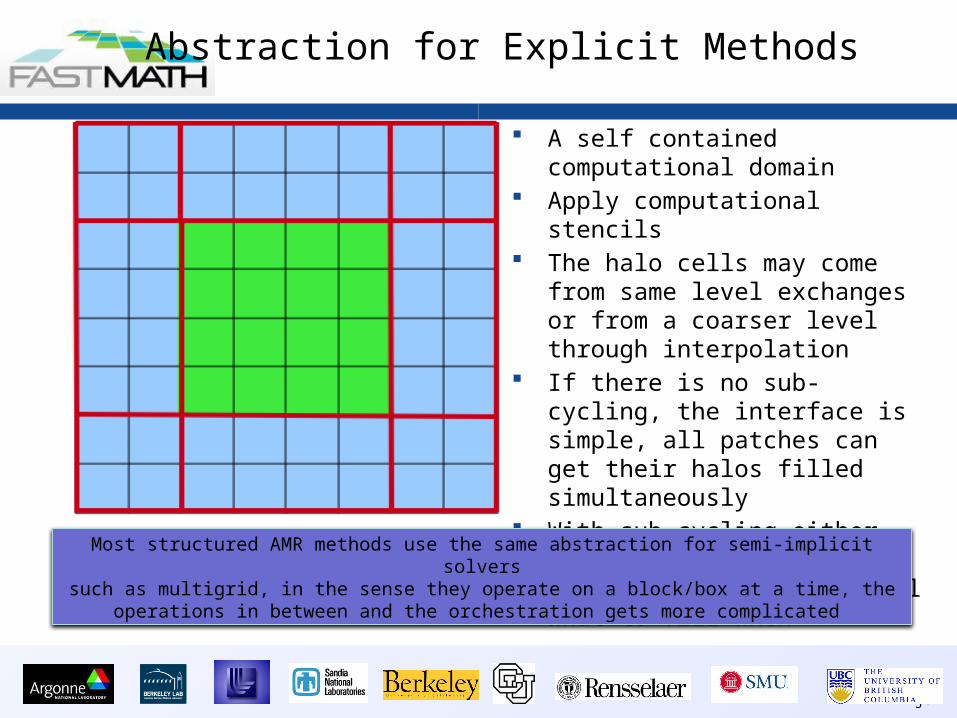
A self contained computational domain
Apply computational stencils The halo cells may come from same
level exchanges or from a coarser level through interpolation
If there is no sub-cycling, the interface is simple, all patches can get their halos filled simultaneously
With sub-cycling either the application or the infrastructure can control what to fill when
Most structured AMR methods use the same abstraction for semi-implicit solverssuch as multigrid, in the sense they operate on a block/box at a time, the
operations in between and the orchestration gets more complicated
Abstraction for Explicit Methods

• Locally refine patches where needed to improve the solution.• Each patch is a logically rectangular structured grid.
o Better efficiency of data access.o Can amortize overhead of irregular operations over large number of
regular operations.• Refined grids are dynamically created and destroyed.
Approach

• Fill data at level 0 • Estimate where refinement is
needed• Group cells into patches
according to constraints (refinement levels, grid efficiency etc)
• Repeat for the next level• Maintain proper nesting
Building the Initial Hierarchy
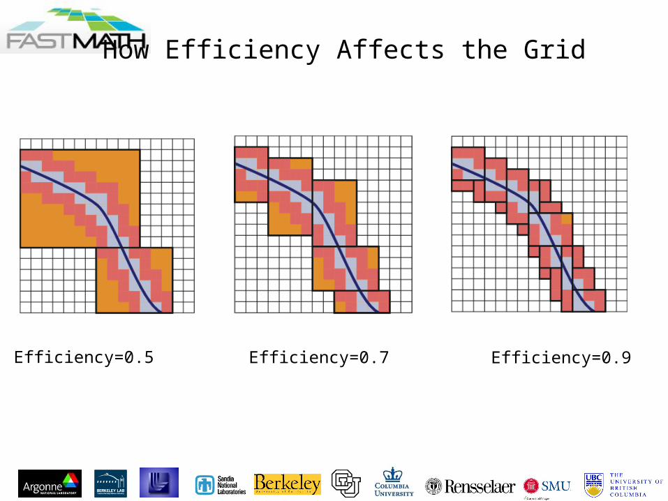
How Efficiency Affects the Grid
Efficiency=0.5 Efficiency=0.7 Efficiency=0.9

• Consider two levels, coarse and fine with refinement ratio r
• Advance • Advance fine grids r times• Synchronize fine and coarse data• Apply recursively to all refinement levels
Adaptive in Time
• Mixed-language model: C++ for higher-level data structures, Fortran for regular single-grid calculations.
• Reuseable components. Component design based on mapping of mathematical abstractions to classes.
• Build on public-domain standards: MPI.Chombo also uses HDF5
• Interoperability with other tools: VisIt, PETSc,hypre.
• The lowest levels are very similar – they had the same origin
• Examples from Chombo
The Two Packages: Boxlib and Chombo
Distributed Data on Unions of Rectangles
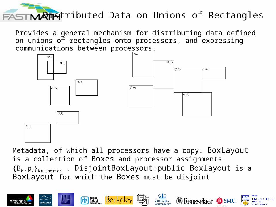
Provides a general mechanism for distributing data defined on unions of rectangles onto processors, and expressing communications between processors.
Metadata, of which all processors have a copy. BoxLayout is a collection of Boxes and processor assignments: {Bk,pk}k=1,ngrids . DisjointBoxLayout:public Boxlayout is a BoxLayout for which the Boxes must be disjoint

Data on Unions of boxes
Distributed data associated with a DisjointBoxLayout. Can have ghost cells around each box to handle intra-level, inter-level, and domain boundary conditions. Templated (LevelData) in Chombo.
Interpolation from coarse to fine
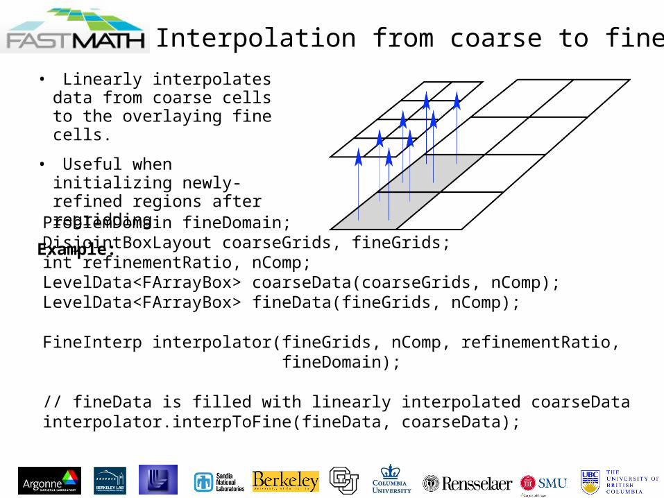
• Linearly interpolates data from coarse cells to the overlaying fine cells.
• Useful when initializing newly-refined regions after regridding.
Example:ProblemDomain fineDomain;DisjointBoxLayout coarseGrids, fineGrids;int refinementRatio, nComp;LevelData<FArrayBox> coarseData(coarseGrids, nComp);LevelData<FArrayBox> fineData(fineGrids, nComp);
FineInterp interpolator(fineGrids, nComp, refinementRatio, fineDomain);
// fineData is filled with linearly interpolated coarseDatainterpolator.interpToFine(fineData, coarseData);

CoarseAverage Class• Averages data from finer
levels to covered regions in the next coarser level.
• Used for bringing coarse levels into sync with refined grids covering them.
Example:
DisjointBoxLayout fineGrids;DisjointBoxLayout crseGrids;int nComp, refRatio;
LevelData<FArrayBox> fineData(fineGrids, nComp);LevelData<FArrayBox> crseData(crseGrids, nComp);
CoarseAverage averager(fineGrids, crseGrids, nComp, refRatio);
averager.averageToCoarse(crseData, fineData);

Coarse-Fine Interactions (AMRTools)
The operations that couple different levels of refinement are among the most difficult to implement, as they typically involve a combination of interprocessor communication and irregular computation.
• Interpolation between levels (FineInterp).
• Averaging down to coarser grids (CoarseAverage).
• Interpolation of boundary conditions (PiecewiseLinearFillpatch, QuadCFInterp, higher-order extensions).
• Managing conservation at refinement boundaries (LevelFluxRegister).

PiecewiseLinearFillPatch Class
Linear interpolation of coarse-level data (in time and space) into fine-level ghost cells.
Example:
ProblemDomain crseDomain;DisjointBoxLayout crseGrids, fineGrids;int nComp, refRatio, nGhost;Real oldCrseTime, newCrseTime, fineTime;
LevelData<FArrayBox> fineData(fineGrids, nComp, nGhost*IntVect::Unit);LevelData<FArrayBox> oldCrseData(crseGrids, nComp);LevelData<FArrayBox> newCrseData(crseGrids, nComp);
PiecewiseLinearFillPatch filler(fineGrids, coarseGrids, nComp, crseDomain, refRatio, nGhost); Real alpha = (fineTime-oldCrseTime)/(newCrseTime-oldCrseTime); filler.fillInterp(fineData, oldCrseData, newCrseData, alpha, 0, 0, nComp);

LevelFluxRegister Class
The coarse and fine fluxes are computed at different points in the program, and on different processors. We rewrite the process in the following steps.
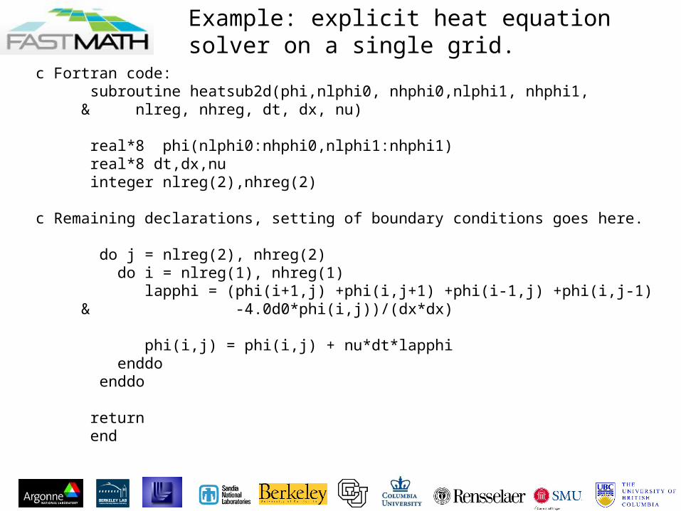
Example: explicit heat equation solver on a single grid.
c Fortran code: subroutine heatsub2d(phi,nlphi0, nhphi0,nlphi1, nhphi1, & nlreg, nhreg, dt, dx, nu)
real*8 phi(nlphi0:nhphi0,nlphi1:nhphi1) real*8 dt,dx,nu integer nlreg(2),nhreg(2)
c Remaining declarations, setting of boundary conditions goes here.
do j = nlreg(2), nhreg(2) do i = nlreg(1), nhreg(1) lapphi = (phi(i+1,j) +phi(i,j+1) +phi(i-1,j) +phi(i,j-1) & -4.0d0*phi(i,j))/(dx*dx)
phi(i,j) = phi(i,j) + nu*dt*lapphi enddo enddo
return end

Example: explicit heat equation solver on a single grid.
// C++ code:
Box domain(IntVect:Zero,(nx-1)*IntVect:Unit); FArrayBox soln(grow(domain,1), 1); soln.setVal(1.0);
for (int nstep = 0;nstep < 100; nstep++) { heatsub2d_(soln.dataPtr(0), &(soln.loVect()[0]), &(soln.hiVect()[0]), &(soln.loVect()[1]), &(soln.hiVect()[1]), domain.loVect(), domain.hiVect(), &dt, &dx, &nu) }
ChomboFortran
ChomboFortran is a set of macros used by Chombo for:
• Managing the C++ / Fortran Interface.
• Writing dimension-independent Fortran code.
Advantages to ChomboFortran:
• Enables fast (2D) prototyping, and nearly immediate extension to 3D.
• Simplifies code maintenance and duplication by reducing the replication of dimension-specific code.
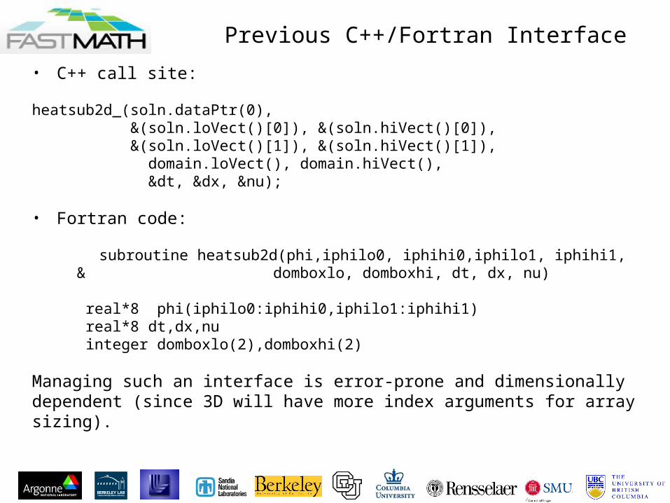
Previous C++/Fortran Interface
• C++ call site:
heatsub2d_(soln.dataPtr(0), &(soln.loVect()[0]), &(soln.hiVect()[0]), &(soln.loVect()[1]), &(soln.hiVect()[1]), domain.loVect(), domain.hiVect(), &dt, &dx, &nu);
• Fortran code:
subroutine heatsub2d(phi,iphilo0, iphihi0,iphilo1, iphihi1, & domboxlo, domboxhi, dt, dx, nu)
real*8 phi(iphilo0:iphihi0,iphilo1:iphihi1) real*8 dt,dx,nu integer domboxlo(2),domboxhi(2)
Managing such an interface is error-prone and dimensionally dependent (since 3D will have more index arguments for array sizing).
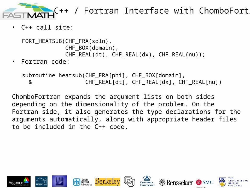
C++ / Fortran Interface with ChomboFortran
• C++ call site:
FORT_HEATSUB(CHF_FRA(soln), CHF_BOX(domain), CHF_REAL(dt), CHF_REAL(dx), CHF_REAL(nu));• Fortran code:
subroutine heatsub(CHF_FRA[phi], CHF_BOX[domain], & CHF_REAL[dt], CHF_REAL[dx], CHF_REAL[nu])
ChomboFortran expands the argument lists on both sides depending on the dimensionality of the problem. On the Fortran side, it also generates the type declarations for the arguments automatically, along with appropriate header files to be included in the C++ code.

Dimension-independence with ChomboFortran
• Looping macros: CHF_MULTIDO• Array indexing: CHF_IX
Replace do j = nlreg(2), nhreg(2) do i = nlreg(1), nhreg(1) phi(i,j) = phi(i,j) + nu*dt*lphi(i,j) enddo enddo
with
CHF_MULTIDO[dombox; i;j;k] phi(CHF_IX[i;j;k]) = phi(CHF_IX[i;j;k]) & + nu*dt*lphi(CHF_IX[i;j;k]) CHF_ENDDO
Prior to compilation, ChomboFortran replaces the indexing and looping macros with code appropriate to the dimensionality of the problem.

Elliptic Solver Example: LinearSolver virtual base class
class LinearSolver<T>
{
// define solver
virtual void define(LinearOp<T>* a_operator, bool a_homogeneous) = 0;
// Solve L(phi) = rhs
virtual void solve(T& a_phi, const T& a_rhs) = 0;
...
}
LinearOp<T> defines what it means to evaluate the operator (for example, a Poisson Operator) and other functions associated with that operator. T can be an FArrayBox (single grid), LevelData<FArrayBox> (single-level), Vector<LevelData<FArrayBox>*> (AMR hierarchy).

• We have seen how construct AMR operator in Chombo as series of sub-operations• Coarse interpolation, fine interpolation, boundary conditions, etc.
• Matrix-free operators• Low memory: good for performance and memory complexity• Can use same technology to construct matrix-free equation solvers
• Operator inverse• Use geometric multigrid (GMG)• Inherently somewhat isotropic
• Some applications have complex geometry and/or anisotropy• GMG looses efficacy• Solution: algebraic multigrid (AMG)
• Need explicit matrix representation of operator• Somewhat complex bookkeeping task but pretty mechanical• Recently developed infrastructure in Chombo support matrix construction• Apply series of transformations to matrix or stencil
• Similar to operator but operating matrix/stencil instead of field data• Stencil: list of <Real weight, <cell, level>>
• Stencil + map <cell, level> to global equation number: row of matrix• Start with A0 : initial operator matrix
• Eg, 1D 3-point stencil: {<-1.0, <i-1,lev>, <2.0, <i,lev>, <-1.0, <i+1,lev>}
Matrix representation of operators
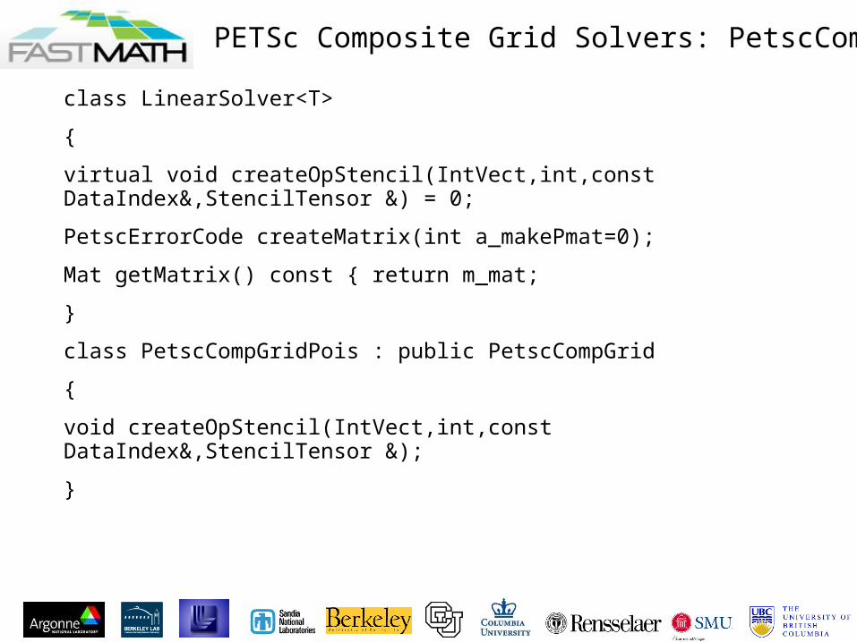
PETSc Composite Grid Solvers: PetscCompGrid
class LinearSolver<T>
{
virtual void createOpStencil(IntVect,int,const DataIndex&,StencilTensor &) = 0;
PetscErrorCode createMatrix(int a_makePmat=0);
Mat getMatrix() const { return m_mat;
}
class PetscCompGridPois : public PetscCompGrid
{
void createOpStencil(IntVect,int,const DataIndex&,StencilTensor &);
}

PETSc Composite Grid Example: PetscCompGridPois
void
PetscCompGridPois::createOpStencil( IntVect a_iv, int a_ilev,const DataIndex &a_di_dummy, StencilTensor &a_sten)
{
Real dx=m_dxs[a_ilev][0],idx2=1./(dx*dx);
StencilTensorValue &v0 = a_sten[IndexML(a_iv,a_ilev)];
v0.define(1);
v0.setValue(0,0,m_alpha - m_beta*2.*SpaceDim*idx2);
for (int dir=0; dir<CH_SPACEDIM; ++dir) {
for (SideIterator sit; sit.ok(); ++sit) {
int isign = sign(sit());
IntVect jiv(a_iv); jiv.shift(dir,isign);
StencilTensorValue &v1 = a_sten[IndexML(jiv,a_ilev)];
v1.define(1);
v1.setValue(0,0,m_beta*idx2);
}}}
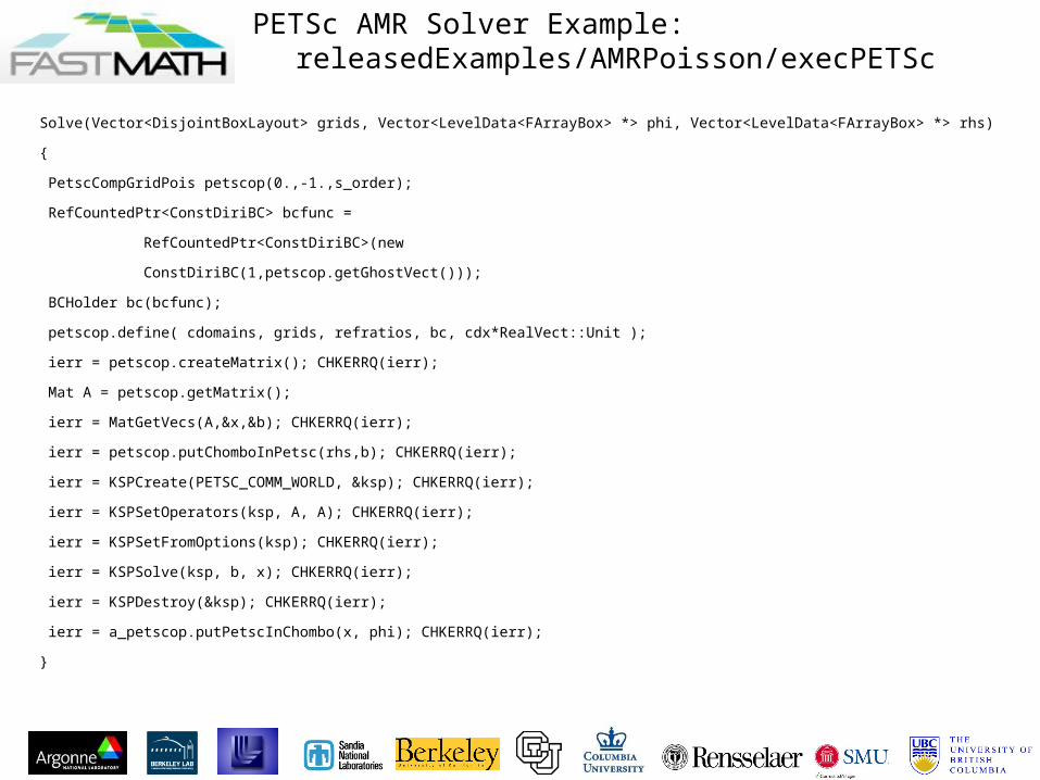
PETSc AMR Solver Example:releasedExamples/AMRPoisson/execPETSc
Solve(Vector<DisjointBoxLayout> grids, Vector<LevelData<FArrayBox> *> phi, Vector<LevelData<FArrayBox> *> rhs)
{
PetscCompGridPois petscop(0.,-1.,s_order);
RefCountedPtr<ConstDiriBC> bcfunc =
RefCountedPtr<ConstDiriBC>(new
ConstDiriBC(1,petscop.getGhostVect()));
BCHolder bc(bcfunc);
petscop.define( cdomains, grids, refratios, bc, cdx*RealVect::Unit );
ierr = petscop.createMatrix(); CHKERRQ(ierr);
Mat A = petscop.getMatrix();
ierr = MatGetVecs(A,&x,&b); CHKERRQ(ierr);
ierr = petscop.putChomboInPetsc(rhs,b); CHKERRQ(ierr);
ierr = KSPCreate(PETSC_COMM_WORLD, &ksp); CHKERRQ(ierr);
ierr = KSPSetOperators(ksp, A, A); CHKERRQ(ierr);
ierr = KSPSetFromOptions(ksp); CHKERRQ(ierr);
ierr = KSPSolve(ksp, b, x); CHKERRQ(ierr);
ierr = KSPDestroy(&ksp); CHKERRQ(ierr);
ierr = a_petscop.putPetscInChombo(x, phi); CHKERRQ(ierr);
}
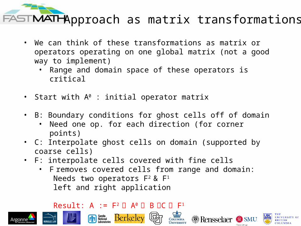
• We can think of these transformations as matrix or operators operating on one global matrix (not a good way to implement)• Range and domain space of these operators is critical
• Start with A0 : initial operator matrix
• B: Boundary conditions for ghost cells off of domain• Need one op. for each direction (for corner points)
• C: Interpolate ghost cells on domain (supported by coarse cells)• F: interpolate cells covered with fine cells
• F removes covered cells from range and domain:Needs two operators F2 & F1
left and right application
Result: A := F2 A0 B C F1
Approach as matrix transformations

• Start with raw op stencil A0, 5-point stencil
• 4 types of cells:• Valid (V)
• Real degree of freedom cell in matrix• Boundary (B)
• Ghost cell off of domain - BC• Coarse (C)
• Ghost cell in domain• Fine (F)
• Coarse cell covered by fine
• “raw” operator stencil A0 composed of all 4 types• Transform stencil to have only valid cells
• B, C & F operator have• domain space with all types (ie, B, C, F)• range space w/o its corresponding cell type
• That is, each operator filters its type• Thus after applying B, C & F only valid cells
remain• Note, F removes F cells from range and
domain:• Needs two operators F2 & F1
• left and right application
Approach from Stencil view
A0 A0B
A0BC F2A0BCF1
Cartoon of stencil for cell as it is transformed
6161
0 1
3 4
211 12
9 10
7 8
5 6
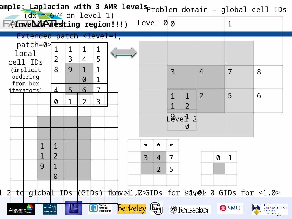
Problem domain – global cell IDs
12 13 14 15
8 9 10 11
4 5 6 7
0 1 2 3
Extended patch <level=1, patch=0>
Level 0
Level 2
Example: Laplacian with 3 AMR levels(dx = 61/2 on level 1)
(Invalid nesting region!!!)
local cell IDs
(implicit ordering from box iterators)
11 12
9 10
level 2 to global IDs (GIDs) for <1,0>
* * *
3 4 7
2 5
Level 1 GIDs for <1,0>
0 1
Level 0 GIDs for <1,0>

6262
-1 -4 -1 -4 20 -4 -1 -4 -1
-1 -4 -1 -4 20 -4 -1 -4 -1
-1 -4 -1 -4 20 -4 -1 -4 -1
-1 -4 -1 -4 20 -4 -1 -4 -1
5
6
9
10
0 1 2 3 4 5 6 7 8 9 10 11 12 13 14 15Initial FABMatrix A0
Local IDs on level 1.Simplify notation:
eg, 5 == <5,1>
I 3x3
I 3x3
I 3x3
*
*
*
5 6 7 9 10
11
13
14
15
FABMatrix B * = -1 for Dirichlet
* = 1 for Neumann.Use higher order
in practice.Split operator into
SpaceDim parts (x & y here).
*
I 3x3
*
*
*
I 3x3
*
I 3x3
*
I 3x3
0
1
2
3
4
5
6
7
891011
12
131415
5 6 7 9 10
11 13
14 15
1 2 3
5
6
7
9
10
11
13
14
15
1
2
3
Bx By

Polytropic Gas Example
• Demonstrates integration of conservative laws (e.g., the Euler equations of gas dynamics) on an AMR grid hierarchy.
• Uses unsplit, second-order Godunov method.• One of the released examples in Chombo distribution• Look under $CHOBO_HOME/releasedExamples/AMRGodonov/execPolytropic• Source code:
• AMRLevel specialized for this set of problems in ../srcPolytropic• Main in ./amrGodunov.cpp• The executable name includes options used in the build
amrGodunov2d.Linux.64.g++.gfortran.OPTHIGH.ex• Compiled using g++ and gfortran• High optimization• For Linux• No MPI
• We use ramp.inputs to provide runtime parameters

Parameters
Length of the run• godunov.max_step = 200• godunov.max_time = 0.064
Shape of the patch• # godunov.num_cells = 32 8 4• godunov.num_cells = 64 16 8
Grid refinement parameters• godunov.max_level = 2# For 2D• godunov.ref_ratio = 4 4 4 4 4# For 3D• # godunov.ref_ratio = 2 2 2 2 2
Regridding parameters• godunov.regrid_interval = 2 2 2 2 2 2• godunov.tag_buffer_size = 3• godunov.refine_thresh = 0.015
Grid generation parameters• godunov.block_factor = 4• godunov.max_grid_size = 32• godunov.fill_ratio = 0.75

Experimenting with Parameters
Default Change ref_ratio to 2
Variations in output with change in refinement parameters


