Download - ANNALEN DER PHYSIK - LSUjdowling/publications/Dowling91.pdf · ANNALEN DER PHYSIK 7. Folge. Band 48. 1991. Heft 7, S. 423-502 Interference in Phase Space ... In the semiclassical

A N N A L E N D E R P H Y S I K 7. Folge. Band 48. 1991. Heft 7, S. 423-502

Interference in Phase Space

J. P. DOWLWG, W. P. SCHLEICH Max-Planck-Institut fur Quantenoptik, Garching bei Miinchen

J. A. WHEELER Department of Physics, Princeton University, Princeton, USA

Abstract . A central problem in quantum mechanics is the calculation of the overlap, that is, the scalar product between two quantum states. In the semiclassical limit (Bohr’s correspondence principle) we visualize this quantity as the area of overlap between two bands in p h s e space. In the case of more than one overlap the contributing amplitudes have to be combined with a phase difference again determined by an area in phase space. In this s e w the familiar double-slit interference experiment is generalized to an interference in phase space. We derive this concept by the WKB approximation, illustrate it by the example of Franck-Condon transitions in diatomic molecules, and compare it with and contrast it to Wigner’s concept of pseudo-probabilities in phase space.

Interfcrenz im Phnsenrsum

Inhaltsubersicht. Ein zentrales Problem der Quantenmechanik ist die Berechnung des Skalar- produktes zweier Quantenzustiinde. Daa Bolusche Korrespondenzprinzip erlaubt eine Darstellung der beiden Zustinde ale Bander im Phasenraum. Die den beiden Biindern gemeinsame Flache ist ein Ma13 fur das Skalarprodukt. Die Quadratwunel aus dieser, geeignet normierten, Fliche represen- tiert den Absolutbetrag der korrespondierenden Wahracheinlichkeitsamplitude. Im Falle mehrerer Durchschnittszonen interferieren diem, wobei deren jeweilige Phasendifferenzen ebenfslls durch Phasenraumgebiete gegeben sind. Dies verallgemeinert das Youngsche Doppelspaltexperiment zu Znterferenz im Phasenraum. Wir leiten dieses Konzept mittels der WKB NiSherung ab, erlautern es am Beispiel von Franck-Condon tfbergiingen in diatomischen Molekiilen und vergleichen es mit der Methode der Wignerschen Phasenraumfunktion.

1. From SchrGdinger’s Wave Function via Hramcrs Phase Space Orbits to Plsnck-Bohr-Sommerleld Bands and Wignor Crests

To look anew at some of the path-breaking papers on quantum theory that appeared in Annulen der Physik in its early days (Fig. 1) is to be reminded of how much these papers taught us. Coming to understand what it is that fixes energy levels was a despe- rate business; this we realize when we look at Planck’s courageous but ill-fated attempt [l] to find a rule to fix the energy levels of a system with many degrees of freedom. To e-uplain the electronic, vibrational, or rotational spectrum of a molecule [2] represented an impossibility until the advent of Schrodinger’s Undulationsmechanik [3], giving birth to the Born-Oppenheimer approximation [4]. Ehrenfest’s paper [5] on adiabatic inva-

424 Ann. Physik Leipzig 48 (l!J91) 7

Fig. 1. Some seminal articles on the structure of phase space and early quantum mechanics that have appeared in Annulen der Physik.

riants RY quantized quantities - expanding his sudden flash of insight a t the first Solvay Congress - shows us an inspiring glimpse into what quantization is all about. Not one of these problems could be treated with the full confidence of obtaining complete accu- racy, with the methods of the ingenious Bohr-Sommerfeld Atommechanik [6--81 alone - exemplified here by the first page of Sommerfeld’s original Annulen der Physik article [O]. A fuller understanding of these problems awaited the advent of the approximation method known most briefly as “WKB”, a stage of development of ideas traced back

J. P. DOWLINQ et al., Interference in Phase Space 425

to Legenclre, Rayleigh and Jeffreys, through Wentzel, Kramers and Brillouin (from which it derives) to Pierce, Klauder and Berry in our own day. They have given this field the name asymptotology [lo].

Asymptotology [ll-201 applies to every field of physics, from atomic and molecular effects [21j, through nuclear phenomena [22], to modern-day quantum optics with its squeezed state technology [23, 241. Asymptotology normally demands smoothness in the potential or an analogous condition of motion - in brief, it capitalizes on problems where rrature does not jump: “natura non facit sa1tum”l) [25]. Therefore nothing might seen1 more paradoxical than using asymptotology to evaluate the quantum mechanical probability of a jump in a sudden transition [26]. To do so however is exactly the purpose of this paper. Asymptotology allows us to understand jump probability associated with the Framk-Condon effect, that is, with a sudden radiative transition of a molecule from one vibronic state to another [2, 27-30]. In nuclear physics [22] i t illuminates the coupling between individual particle motion and collective degrees of freedom. In quantum optics it predicts the now eagerly sought oscillations in the photon count probability distribution of a squeezed state of the electromagnetic field [31, 321. Out of these three representative areaa of physics we choose here the Franck Condon effect as the most suited to illustrate how jump probability operates: by interference in phase space [all.

1.1. Franck-Condon Transitions in a Diatomic Molecule

Ever since the pioneering work2) carried out by James Franck 1271 and Edward Condon [28, 291 (Fig. 2) it has been known that certain vibrational levels are preferentially excited in the radiative transition of a diatomic molecule from one electronic state. Why? The reason for - and the requirement of - high transition probability is the

I ) The Homebook of Quotations by B. Stevenson (Sew York: Dodd and Mead 1934) attributes this quotation - translated there as “Nature does not proceed by leaps” - to Carl Linnaeus ( 1 i O i bis 1778), who made this statement in Sec. 77 of his book, Philosophia botanica. Linnaeus or van Linnh was a Swedish botanist who held a chair in Uppsala as a professor of medicine. More about his life can be found in: Dictionmy of 8cientific Biography (edited by C. C. Gillispie). New York: Scribner 1980.

1) To unravel the occupation probability of electronic, vibrational, or rotational states in a diatomic molecule - on first sight an insurmountable problem - simplifies considerably when me recall the Born-Oppenheimer approximation [4]: The nuclei, due to their large mass move slowly compared to the electrons. Hence the nuclei remain a t their instantaneous position and keep their momenta during an electronic transition, that is, the intermolecular potential changes suddenly. J. Franck, anticipating this yet to be discovered Born-Oppenheimer approximation, and solely based on this notion of a sudden transition, explained [27] the radiative dissociation of a diatomic molecule as a sudden change of the binding potential from attractive to repulsive - in today’s language, a trsn- sition from the vibrational ground state to the continuum. E. Condon recognized [28, 291 that this explanation appliea to more than the ground state. He argued that the jump from a highly excited vibrational state is equally likely for any phase of the vibratory motion of the nucleus. Since the nucleus spends more time a t the turning points of its oscillatory motions) - because there the momentum is zero - the transition will happen preferentially at the turning points. R. Mulliken [30] extended this principle to the case of jumps taking place at positions different from the turning points. H e postulated that the transition occurs at positions where the kinetic energy of the final orbit is identical to that of the initial one. His dqjeerencc potential, illustrated in Fig. 11, allows one to find these positions. This requirement of conservation of kinetic energy is identical to the crossing condition, Eq. (2.7), of the two Kramers orbita.

426 Ann. Physik Leipzig 48 (1991) 7

Fig. 2. James Franck (left) and Max Born (right) in Gottingen in the twenties (left figure). Edward Condon (left) with H. P. Robertson (right) in Princeton in the thirties. (Courtesy of American Institute of Physics, Niels Bohr Center)

identity of the classical turning points [2, 28, 291 for the vibratory niotions in the initial antl final states, as indicated in Fig. 3 a by the vertical, broken line^.^)

Transition probabilities are not zero for vibrational states such as the states m antl n that fail to meet this demand for identity of the turning points. On the contrary, the probability curve is similar [33--381 to a catenary curve - the same curve a rope follows when it is suspended from both ends. This catenary is, however, modulated by a high frequency variation from one quantum state to the next, as shown in Fig. 3b. Nowhere more than in looking at such a striking pattern of intensity variation are we reminded once again of the interference pattern obtained in the familiar Young double-slit experiment 139-411. Interference? Yes! But interference where ? What and where are the two slits in the Franck-Condon problem ?

Is the standard formalism of quantum mechanics [26] of any immediate help in answering these questions ? This formalism restates [2] the probability for a transition to occur from the nth vibrational state of a diatomic molecule in one electronic state to the mtli vibrational level of a different electronic state, as

wm,n = I%,nla 9 (1.la)

3) We recall here the familiar parable of the turning point. The four-year old unexpectedly sweeps the aim of the lawn hose to the right - raking the jet of water over the circle of unwary admirers - then again to the left, before he drops it. The turning point of the sweeping motion sepa- rates the wettest victim from her dry neighbor. “What a mess”. Wetness in this incident models position probability for a particle reflected at a turning point.

J. P. DOWLING e t al., Interference in Phase Space 4 2 i

t ha t is, as the square of the Franck-Condon factors

Wm.,, = y dxu,(x) V J X ) . -0J

Thus Wrn.,, is governed by the overlap of, that is, t

2, 27-30]

( l . l h )

,e quantum niechanical scalar product between, the two vibrational wave functions urn and v, in position (or x) space.4) No indication of the two slits! They are hidden behind this “mist” of formalism.

1.2. Jump Probability via WKB, Area of Overlap or Wigner Functions ?

The answers [el] to these questions are founcl in Fig. 4, which summarizes the approach of asymptotology. Everything in this paper leads up to and springs forth from this fignre. The formal verification of these statements will come in the later sections, but at the present stage we want to point out all of the beauty, all of the surprises, and all of the connections between these asymptotological answers and other points of view. In particular we focus on a , on first sight, estremely troubling point, the resolution of which illustrates in a striking way the different approaches to evaluate jump probabilities and the quantum mechanical scalar product via asymptotology.

What i s the range of x values that determines the overlap integral, Ey. ( l . lb) , between the two vibrational wave functions urn and v,? (1) The total x axis, (2) a well- defined interval of x values, or (3) a single point 2,: three seemingly contradictory answers to the same question, and nevertheless all three replies are correct. How can we possibly resolve such a paradox ? We resolve it by recognizing that the three different answers represent three different levels of appioxinintion to wm,,.

The definition of IL ;~ , , , Eq. (L lb ) , asks us to perform the integration of the product of the two wave functions along the complete x axis, that is, from minus infinity to plus infinity. For large quantum numbers m and n the two waves u, and v,, are rapidly varying and their product u, . v, is highly oscillatory, as indicated in Fig. 4a that incor- porates the esaniple of two harmonic oscillators of identical (unit) frequency that are displaced by an amount x,, = 12, as depicted in Fig. 5a. These rapid oscillations might seem to totally compensate, giving us a zero result for wrn,,. However, the esact calculation [42, 431 predicts a nonvanishing value. How to distill out of this “roller- coaster” product urn. v, the nonzero contributing part - that is the first problem w e face. Represent the two energy eigenfunctions by two WKB cosine waves of rapidly varying phases, that is the approach which immediately allows insight into this “mist”. The product of these two waves is the sum of two waves whose phases are the sum and the difference of the individual phases. The term containing the sum of phases oscillates rapidly and gives approximately zero when integrated over x, whereas the difference- phase term, shown in Fig. 5c, when evaluated with the help of the method of stationary phase, [44] yields a nonzero contribution, if any. The contribution to this integral, Eq. ( l . lb ) , from the 2 values of the highly oscillatory regime averages out. Only the domain Ax(=*) around xc, given in Sec. 2 and in Table 1, counts as important determiner of the value of w,,,. This point x, is the position coordinate of the crossing point,

4 ) Throughout this work we use the dimensionless coordinate x E ( , ~ w / E ) ~ l ~ q and momentum p = (ptlw)- ‘I2 5 insteadof the variables q and 5 whichdescribe a particle of nmss p moving in a potential 5 = &). The frequency w is some typical frequency. I n these dimensionless variables, the ener-

gy E =2/ (2y) + 6(q) reads = -pa + U(x), where the dimensionless energy is defined as 7 = l / ( f w ) E, and the potential V(s) = l / ( fo) 6{[n/(po)]’ l2 2).

1 2

428 Ann. Physik Leipzig 45 (1991) i

I I J 6 9 12

- (b)

5

t I P

- S

Fig. 3

Fig. 4

J. P. DOWLIXG e t al., Interference in Phase Space 429

shown in Fig. 4b, between the two Kramers phase space trajectories5)

(1.2a)

(1.2 b)

5) We describe the semiclassical motion corresponding to the mth level of potential U ( l ) by the momentum p$ = p , and analogously of the nth level of U(’) by p:) = p,. To keep the notation simple we have suppressed the index 1 or 3; in the remainder of the article pm always refers to potential t?(’) and p,, to potential U(2).

Fig. 3. Franck-Condon transitions from the nth vibrational level of the upper electronic state, with intermolecular potential U(2) , to vibrational states m in the lower electronic state, with potential U(I) . The two final vibrational levels of the lower electronic state (shown by solid lines) have the turning points 5, nnd x,, in common with the nth vibrational motion of the upper electronic state and are, according to the Franck-Condon principle, prefered final states. (We can see this by noting the maxima a t m = rnn,in and m = malnpx in (b).) For levels m between these two Frunck-Condon maxima, the catenary curve of jump probability is modulated (see Refs. 34-38).

Fig. 4. Four methods to evaluate jump probability W,,,,, in a diatomic molecule compared and contrasted. The exact expression for w ~ , ~ , Eq. (l.lb), we obtain from integrating the product of the two vibrational wave functions u, and vn, depicted in (a), over all positim space, that is, along the entire x axis. The method of stationary phase, when applied to the product uhmB)(x) . vPmB)(x) of WKB-approximated waves, shows that the main contribution to the integral w,”,, arises from the crossing points of the corresponding Kramers trajectories Ip I = p,,, and ( p I = pn, Eqs. (1.2). Hence the integral stems from wave behavior a t two well-defined phase spacepoints, and in particular, a t the single x value xc, as shown in (b). However, the magnitudes of the probability amplitudes corresponding to these crossings - governed by the angle between the two Kramers orbits, Eq. (2.12) - are only obtained after integrating the Taylor-expanded phase, Eq. (2.9a), over all position space. The area of overlap apprmh, indicated in (c), relates the jump probability to the two, diamond-shaped, phase space m a of cross-over between the two Planck-Bohr-Sommerfeld bands - bands which are the phase space representatives of the two states. In contrast to the methods of (a) and (b), here only the small interval of x valuea within the diamonds provides the WKB value of the overlap integral w,,,,, Eq. (Llb). Similar to the concept of area of overlap, the W i p e r function technique of (d) determines the jump probability via well-localized, finite donlains in the neighborhood of the phase points (xc, f pm(xc)). Here, however the range of x values and p values giving rise to the WKB probability amplitude w,,, is quite different from the range in the other three techniques, and in particular, significantly larger than in (c). The fact that the phase space weight factor is smaller here than it is in (c) compensates for the larger phase space domains; thus the resul- tant probabilities turn out t . ~ be identical. For definiteness we have chosen in these examples the energy wave func t ions~ , ,~~ and V , , ~ ~ ( X ) = U , - ~ ~ ( X - x,,) of two identical harmonic oscillators of unit frequency, Eq. (A2), which are displaced by an amount z,, = 12.

430 Ann. Physik Leipzig 48 (1991)

, 1

0 --x- 5 10 x o

Fig. 5. Extraction of the minimally oscillating component of the product of two wave functions. The probability for a sudden transition from the 1c = 18th level of a harmonic oscillator of unit frequency to the m = 58th state of an identical oscillator displaced by an amount z,, = 12 (a) is governed by the overlap between the two corresponding wave functions u,,+~*(z) and = un=ls (2- xo) depicted in (b). The product of these highly oscillatory functions, shown by the lowest curve in (b) varies rapidly in the domain caught between the turning points of the corresponding classical motions. Only when we decompose each wave into two counter-propagating waves and combine the right-going component of urn with the left-going wave of vll and add its counterparts. do we distill out of the noisy product urn * v,, its most quiescent component, that is, the slowest varying part - shown in the top curve of (c). In the neighborhood of xc = 9.33 this contribution is least noisy. The method of stationary phase identifies this point as the position coordinate of the crossing point of the two, circular, Kramen p+ space orbits corresponding to the two levels of intemt. These two orbits, depicted in (d), are given by 2(m + 1/2) = 117 = pe + x2 and 2(n + 1/2) = 37 = pz + (x - 12)s. Away from the point x, rapid oscillations of the integrand of the overlap integral, Eq. (l.lb), make contributions that approximately cancel each other. Hence the decisive part of the integral arises from the neighborhood of z,. This is the rationale for approximating the product urn@) - v,,(z) by the quadratically Taylor-expanded, oscillatory function Eq. (A15) - the curve in the middle of (c). The integral over this function, depicted by the lowest curve in (c), oscillates as a function of the position variable x while it approaches the steady state limit given by Eqs. (2.11) and (2.15). This limit is obtained by integrating along the total z axis.

Tab

le 1

. R

oute

to

jum

p pr

obab

ility

via

pro

babi

lity

ampl

itude

s in

po

sitio

n sp

ace,

or

inte

rsec

ting

Plan

ck-B

ohr-

Som

mer

feld

ban

ds

and

Wig

ner

cres

ts,

repr

esen

ting

dire

ctly

the

cor

resp

ondi

ng p

roba

bilit

ies.

(The

mom

enta

pm

and

p,,

and

thei

r der

ivat

ives

wit,

h re

spec

t. to

pos

ition

, de

note

d by

pr

imes

, are

eva

luat

ed a

t the

cro

ssin

g po

int z

c of

the

two

Kra

mer

s tr

ajec

tori

es. T

he p

erio

ds of

th

e tw

o en

ergy

eig

enst

ates

are

T,,,

and

T,, r

espe

cti-

ve

ly.)

appr

oach

Po

sitio

n Space:

Phas

e Sp

ace:

Ph

ase Space:

rout

e to

W

KB

ar

ea o

f ov

erla

p W

igne

r fun

ctio

n ju

mp

prob

abili

ty

(pro

babi

lity

ampl

itude

) (c

ross

-ove

r of

band

s)

(tor

oid

appr

oxim

atio

n)

area

in

phas

e sp

ace

wA

xA

p

-

3

a r

6'

432 ilnn. Physik Leipzig 48 (1991) i

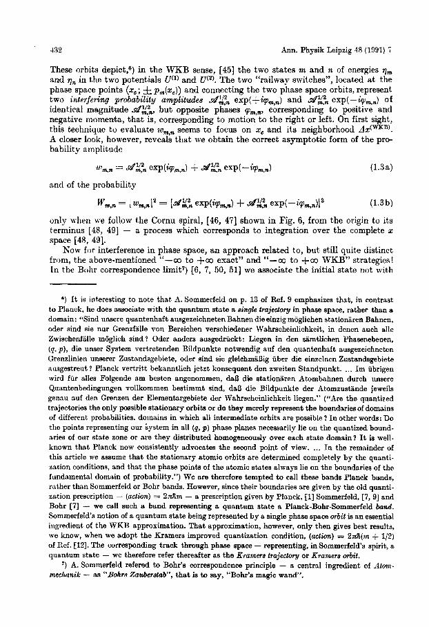
These orbits depict,”) in the WKB sense, [45] the two states m and n of energies qm and vn in the two potentials Uc1) and U(2). The two “railway switches”, located at the phase space points (2, ; -J= p,,Jx,)) and connecting the two phase space orbits, represent two interfering probability amplitudes dz.“, exp(+iFrn,+) and dz ; exp(-iqJ,,,! of identical magnitude at$,:, but opposite phases vrn,n, corresponding to positive and negative momenta, that is, corresponding to motion to the right or left. On first sight, this techniquc to evaluate w,,~ seems to focus on x, and its neighborhood Ax(WKB’. A closer look, however, reveals that we obtain the correct asymptotic form of the probability amplitude

and of the probability

(1.3a)

(1.3b)

only when we follow the Cornu spiral, [46, 471 shown in Fig. 6, from the origin to its terminus [48, 491 - a process which corresponds to integration over the complete x space [48, 491.

Now for interference in phase space, an approach related to, but still quite distinct from, the above-mentioned “-00 to +co exact” and “-00 to fa WKB” strategies! In the Botir correspondence limit’) [6, 7, 50, 511 we associate the initial state not with

6 , It is interesting to note that A. Sommerfeld on p. 13 of Ref. 9 emphasizes that, in contrast to Planck, he does associate with the quantum state a single trajectory in phase space, rather than a domain: “Sind unsere quantenhaft ausgezeichneten Bahnen die einzig mijglichen stationaren Bahnen, oder clind sie nur Grenzfalle von Bereichen verschiedener Wahrscheinlichkeit, in denen anch alle Zwischenfille moglich sind ? Oder anders ausgedriickt : Liegen in den siimtlichen Phasenebenen, (4. p), die unser System vertretenden Bildpunkte notwendig anf den quantenhaft ausgezeichnctcn Grenzlinien unserer Zustandsgebiete, oder sind sie gleichmll3ig iiber die einzelnen Zustandsgebiete ausgestreiit ? Planck vertritt bekanntlich jetzt konsequent den zweiten Standpunkt. .. . Im ubrigen wird fur alles Folgende am besten angenommen, daB die stationiiren Atombahnen durch iinsere Quantenbedingungen vollkommen bestimmt sind, daB die Bildpunkte der Atomzustlnde jeweils genau auf den Grenzen der Elementargebiete der Wahrscheinlichkeit liegen.” (“Are the quantized trajectories the only possible stationary orbits or do they merely represent the boundaries of domains of different probabilities, domains in which all intermediate orbits are possible? I n other words: Do the points representing our iystem in all (p, p) phase planes necessarily lie on the quantized boundaries of our state zone or are they distributed homogeneously over each state domain? It is well- known that Planck now consistently advocates the second point of view. ... I n the remainder of this article we assume that the stationary atomic orbits are determined completely by the quantization conditions, and that the phase points of the atomic states always lie on the boundaries of the fundamental domain of probability.”) We are therefore tempted to call these bands Plenck bands, rather than Sommerfeld or Bohr bands. However, since their boundaries are given by the old quantization prescription - (action) = 2nZm - a prescription given by Planck, [l] Sommerfeld, [7, 91 and Rohr [7] - we call such a band representing a quantum state a Planck-Bohr-Sommerfeld band. Sommerfeld‘s notion of a quantum state being represented by a single phase space urbit is an essential ingredient of the WKB approximation. That approximation, however, only then gives best results, we know, when we adopt the Kramers improved quantization condition, (&ion) = 2nfi(m + 1/2) of Ref. [El. The corresponding track through phase space - representing, in Sommerfeld’s spirit, a quantum state - we therefore refer thereafter as the Rramers trajectory or Kramers urbit.

’) A. Sommerfeld refered to Bohr’e correspondence principle - a central ingredient of dtom- mechanik - as “Bohrs Zauberstab”, that is to say, “Bohr’s magic wand”.

J. P. Dow~xxa et al., Interference in Phase Space 433

- 0.5 c

0.5 -E ly ) - I

Fig. 6. The Cornu spiral - prameterized by its path length y and obtained in Cartesian coordinatcs from the Fresnel integrals

U U(y) = j. dt cos(nl~/B)

0 and

U ~ ( y ) =I 1 dt sin(nt”2)

n allows us to discuss geometrically the influence of the neighborhood 6% of zc on the value of each of the probability amplitudes contributing to w,,,,. These amplitudes have a magnitude R(y) and a phase ,8(y), which correspond respectively to the distance between a point at y = a 6% on the spiral and the origin, and this point’s angular position relative to the asis. The quantity a is closely related to the angle at which the two Kramers orbits cross each other. When we increase Sx, that is, when we increase the parameter y, the quantities R and /3 oscillata and converge, in the limit of y = a 62 - 00, towards steady-state values. I n this case R ( w ) and P(m) are the polar coordinates of the center of the spiral with respect to the origin. These limiting coordinates are, for the magnitude, R =

[(1/’2)2 + (1/2)2J1’2 = l /f2 and, for the angle, /3(m) = 4 4 . The convergence towards these values - one loop after another, one Fresnel zone after another - is slow - “convergence without convergence.” This slowness is a happy feature of the “method of interference in phase space.” It tells 11s

that it matters little for the final transition probability exactly how the latter loops spiral inward, it matters little how the wave functiona vary - if they vary slowly - outside of the zone of constructive interference, that is, of the caustics of the bands in phase space.

-

a single phase space orbit, but rather with a band6) [ l , 21, 24, 31, 32, 521 in phase space of area 2n (in units of Dirac’s constant ti). Likewise, we represent the final state by its own domain, as show-n in Fig. 7. We evaluate the area of overlap of the two domains

divide by 2n, and take its square root. The result governs the amplitude of transition from the initial to the final state. When there is more than one intersection, then there is more than one such amplitude, more than one “reaction channel”. Then the amplitudes - now regarded as complex numbers - must be added with due regard of phase to get the total amplitude for the transition. No absolute phase needs to be defined for any channel contribution individually. Only phase differences count. The phase difference between the contributions for two channels is governed [21] by the area in phase space caught between the initial and final orbit, shown in Fig. 8.


0 XO -X-- I Fig. 7. A sudden transition: Tools for figuring the transition probability - illustrating the ties between classical theory and quantum theory. Below: The curves for potential energy as a function of the position coordinate x before the transition (above) and after the transition (slightly lower). The horizontal lines indicate allowable energy levels in these potentials before and after this transition. The wave functions u, and v,, shown here belong to the initial and final states between which we wish to evaluate the transition probability via an integral of the form

J urn@) x (slowly varying function of x) x v&) dx.

Top: Bands in phase space (shaded) associated with initial and final state, and the area of overlap between them (blackened). This area of overlap is a tool for determining - in the semiclassical approximation - the transition probability.

This very idea of area in p h s e $pace as a determiner of transition amplitudes, together with the concept of interference in phase space as a generalization of the familiar double- slit experiment8) - the topic of See. 3 as summarized in Fig. 8 and the box - suggests that only a well-defined regime of x values Ax(PBS), discussed in See. 3 and represented in Table 1, determines the overlap integral w ~ , ~ . This is in strong contrast to the exact

8 ) The double-slit experiment summarizes most clearly the central lesson of quantum mechanics: Probabilities a t the microscopic level are governed by interfering probability amplitudes rather than by additive probabilitiea. The importance of probability amplitudes rather than probabilities is em- phasized in the path integral formulation of quantum mechanics [40,41] and in the concept of interference in phase space [%, 24, 31, 321.

J. P. DOWLING et al., Interference in Phase Space 435

Fig. 8. The area-of-overlap concept. I n the semiclassical approximation (Bohr’s correspondence principle) the quantum mechanical scalar product w , , ~ between two stationary states urn and vn can be visualized as the overlap between the two states depicted in z -p oscillator phase space as occupied bands traversed in a clockwise direction. I n the case of more than one such overlap (in the present example, two) the two, diamond-shaped, dark areas differ in their “momentum”: I n one dark zone both oscillators move to the “right”, whereas in the other to the “left”. Thus the total probability amplitude wm,, is the sum of contributions afi; exp( -++,,,) from the two zones. Here the phase v, ,~ is fixed by the shaded area caught between the center lines of the two states. No simpler illu- stration presents itself for interference in phase space.

calculation and the WKB approximation. In the case of the two displaced harmonic oscillators, this interval of x values is distinctly smaller than the width Ax(-) of the dominant maximum of the oscillations around xc as indicated in Fig. 4c.

Box I: Transition Probability b y Method of Interference in Phase Space

Wm,n = 4 - (areal) x cos2(area2)

W,,, = probability of transition between states of quantum numbers m and n;

area1 = one area of intersection between the two Planck-Bohr-Sommerfeld bands expressed

areaz = area embraced by the two center lines of the two bands expressed in unita of ti =

in units of h = 2&;

h / ( W ;

Interfering areas of overlap in phase space as a measure of interfering transition probability amplitudes: this concept brings to mind Wigner’s phase space function, [53-561 the subject of Sec. 4. This framework, however, does not deal with interfering probability amplitudes giving rise to wm,, but provides directly the probability Wm,n = I w,,,I2, Eq. (1.la). The overlap between the Wigner functions Pkm and F’$$W - pseudo-phase- space probabilities for the two states of interest - when integrated over the total phase space, yields the probability W,,,, Eq. ( l . l a ) , that is, [56-581

Q) m

Wm,n = 2~ J J d p P P ( x , PI PP’)(x, PI * (1.4) -a3 -m

436 Ann. Physik Leipzig 4’3 (1991) 7

Fig. 9. Product of two Wigner functions P~W=)&z, p) and P i T 1 8 ( z , p ) , as tools to determine the probability Wm158,n318 for a sudden transition (Fig. 5a) from the n = 18 t h state of harmonic oscillations about 2, = 12 to the m = 58 t h state of oscillations about the origin. Two peaks, or Wigner crests, identified by arrows and located near xc = 9.33 and +p,(z,) = & 5.5 dominate the landscape of the product function. The integrated volume under these peaks yields the “classical” jump probability @Cl) m,n - - peak) m,n = 2dm,,, Eq. (4.15). analogously to the two diamond-shaped zones of band overlap of the area-of-overlap approach. The ‘‘wavy sea” between the two peaks, with all its wave crests and troughs where this product of pseudo-probabilities assumes negative as well as positive values, contains the interference between these two peaks. We integrate the volume under this ‘sea’ to find WLT) = 2dm,n cos(2pm,,).

Figure 9 illustrates the ’CTiigner function approach for the, by now, familiar example of two harmonic oscillators. We recognize two dominant maxima, located in the neighborhood of the crossing of the two circular Kraniers phase space orbits, from Fig. 4b. These peaks are the counterparts of the skewed “slioeboses”, or “skewboxes”, of the area of overlap approach of Fig. 4c. We note that, in contrast to the methods underlying Figs. 4a and 4b, here the probability W(,Peik) caught underneath these peaks, shown in Fig. 4d, without the “wavy sea” of Fig. 9, is determined by well-defined, weighted areas in phase space. Hence only a limited interval of z values and also of p values contributes to the probability 2W$,%k) = corresponding to the two peaks. How-

ever, the base or “ground base” of those peaks, -A&?, is broader than that of the

area of overlap approach, TA$zs), as compared in Table 1. Identical jump probabi-

lities 2 d m , , result because the two weight functions are different: the height of the Wigner peak is smaller than that of the Planck-Bohr-Sommerfeld band.

The Wigner function approach deals in terms of (pseudo-) probabilities. Interference effects must therefore originate from phase space domains where the Wigner function product PLw. PnW assumes negative values. The phase space area below the wavy sea, caught between the two positive-valued peaks (shown in Fig. 9), yields the pseudo- probability Wg$, which follows from Eq. (1.4) when we recall that

l 2

1

wm,n = 2 W Z t k ) + WLT) = wm,n + we:)

J. P. DOWLIXG e t al., Interference in Phase Space 437

and Eq. (1.3b), which yields

(1.5)

Nowhere clearer do we see once again the similarities and differences between the approach of interference in phase space and the Wigner function technique than in Eqs. (1.3 b) and (1.5): interfering areas in phase space representing probability amplitudes versus positive- or negative-valued areas in phase space expressing probabilities, that is a one sentence summary of this section.

In order to keep the article self-contained, we include all relevant calculations - but banish the lengthy ones to the appendices. Moreover, me introduce boxes at the beginning of each section which summarize the key ideas with clarity.

2. Jumps a la WKB

2.1. Quantum Mechanical Transition Amplitude Translated into the Languagc of Cornu's Spiral

A quantum mechanical system esposed to a sudden change of contlitions undergues a jump from state n to state m with a probability amplitude

The same factor governs [2, 36,371 the probability amplitude for the radiative tramition of a molecule from one vibronic state to another when the dipole moment's variation with internuclear separation, x , is small over the range of x values that contribiite importantly to the matrix element. We do not ask here how to derive this well known standard result, but how to discover whether w, , ,~ is big or small, and what makes it

No obstacle to such an insight looms larger than the mix of contributions hidden in Eq. (2.1). Each of the two wave functions we picture as itself the conibination of two waves, one marching to the left, the other to the right. Never by scrambling them all together - as a numerical esample illustrates (Fig. 5.) - can we capture the essence of the action. Take, however, the right-traveling wave of urn, multiply it by the left- traveling wave of v,, and add the converse combination of waves - then plot this all up in Fig. 5 c. There stands out in this curve the essence of the jump-governing amplitude. The thrust of the probability amplitude concentrates itself in a limited domain of the coordinate x. (No such domain of quiescent phase appears when we multiply the right- traveling wave of urn and the right-traveling wave of v,,, or multiply the two corresponding left-traveling waves - and therefore from them we do not get a significant probability for the transition.) Surrounding this region to the left and right are domains where the contributions alternate in sign so rapidly that they cancel out. This behavior is familiar from physical optics [47,59]. In propagation of light, the amplitude of the electric field at the place of observation takes the place of the probability amplitude of Eq. (2.1). Transverse distance along the contributory wave front is the appropriate interpretation for the coordinate x. The addition of contributions from all along the wave front expresses itself in the integration over x . Contributions from the center of the wave

so.

-


front combine in constructive interference; they dominate. The total range of x, to be sure, is infinite. However, the contributions from outside the range of constructive interference cancel out, as illustrated so beautifully in the familiar Cornu spiral shown in Fig. 6. It is decisive for this cancellation that phase varies quadratically, or nearly so, with departure from the center of the wave. That’s why the contributions from the outlying regions slowly wind up to the center of the Cornu “snail” - this is an example of “convergence without convergence”. The situation is similar here, expect that the details of wind-up at the center of the snail deviate in unimportant ways from the exact Cornu prescriptioir.

-

2.2. WKB Illuminates Probability Amplitude tor Jump

Approximate the wave functions urn and v,, by their WIG3 expressions and then evaluate the integral, Eq. (2.1), with the help of stationary phase; that is the approach suggested in Sec. 2.1 and by Landau many years ago in the context of energy transfer in collisions [60], pursued successfully in many different physical problems [Gl- 641 and reviewed in this section with the emphasis on an interpretation in phase space [38, 461.

In t.he semiclassical limit, 111-181 that is, for large quantum numbers m the wave functions urn can be approximatedg) [12, 14, 16,171 in the region between the two classical turning points 1 9 ~ and Ern, (t?,,, < &,,, see Fig. 10) by the WKB wave functions

(2.2a) u~-’(x) = Nrnp,‘*(z) COS[&(Z) - n/4]

where

Prn(s) {2[qrn - U(’)(Z)])+ (2.2b)

and

(2.2c)

The energy q, of the mth eigenstate of the potential U ( l ) = U(’)(X), shown in Fig. 10a, is determined by the Kramers quantization condition [12] of a half quantum of area in phase space,

Jrn=$cZxprn(x)=2z m + - . (2.2d)

9) This simple procedure breaks down for quantum states m which cut the elliptical n-band of Fig. 1Oc tangentially. This situation corresponds to Franck-Condon transitions around m,,,, and mmax of Fig. 3, at the turning points of the classical motion. Here the WKB waves, Eqs. (2.2) and (2.3), turn singular and a uniform asymptotic expansion [66] of urn and u, is necessary. Such a treatment can be found in Ref. [SZ]. Since the goal of the present article is to bring out the conceptual points of the phase space interpretation of semiclassical techniques, such as the area of overlap approach of Sec. 3 or the concept of the Wigner function, summarized in Sec. 4, we restrict ourselves to quantum dcates m which lie between mmin and mmax of Fig. 3, that is, to m bands which cut two symmetrically located diamonds out of the n band. For these m values, this approach yields good agreement with the exact treatment, as exemplified in Appendix A for the case of two displaced harmonic oscillators. For the more sophisticated treatment based on a WKB wave function, valid along the complete x axis, we refer to Ref. [SZ].

( 3

J. P. DOWLIWG et el., Interference in Phase Space

I

I

439

Fig. 10.

440 Am. Physik Leipzig 48 (1991) 7

The normalization constants N,,, follow from Eq. (2.2a) as C

1 = N: j- dxp;lco$ . *m

1 C 1 1 = - M i $ dZp,’(x) = - 2 2 T,,

*m

that is,

N, = 2Ti* .

Here

C T, = 2 1 dzpk l (x ) = p d t

am

(2.2e)

(2.2f)

is the period of the mth orbit. Analogously we approximate [12, 14, 16, 171 the wave functions v,, = v,(x) for 2

values appropriately between the classical turning points gn and xn (qn < xn, see Fig. 10a) by

(2.3a)

(2.3b)

(2 .3~)

Fig. 10. Area-of-overlap method to evaluate jump probability, briefly recapitulated. (a) Potential of the force under which a system oscillates, depicted as a function of coordinate 2, before (U(2) , with minimum at zo) and after (U(’), with minimum a t x = 0) the sudden change in the conditions of motion (capital example: vibration of a diatomic molecule as affected by an electronic transition). Also shown in (a) are the energy level and wave function for the original vibration state n and for a sample one m of the many f m l statea that compete for attention. (b) Phase space trajectories m and n of candidate final state m and given initial state n, as determined from the Kramers quantization rule: The area enclosed (in units of W ) is equal to 2n(m + 1/2) and 2n(n + 1/2), respectively. (c) Initial state and candidate final state depicted as Planck-Bohr-Sommerfeld bands of area 2n (in units E ) . The two symmetrically located diamond-shaped zones of intersection between bands n and m serve as the two “slits” of the “phase space-double-slit experiment,” the outcome of which governs the transition probability Wm,n. The sum of transition probabilities from n to all final states m, when accurately calculated, adds exactly to 1, as expected from the unit area (in units of h = 2xfi) of the nth initial-band. When the band for the candidate final state makes a tangential intersection with the band for the given initial state, as happens in the neighborhood of the turning points z = c,, and z = x,,, i t has an unusually large overlap with the initial-state band (shaded areas) and, according to the area-of-overlap-concept, yield a large transition probability in agreement with the Franck-Condon principle (see Fig. 3).

J. P. D O ~ L I N G et al., Interference in Phase Space 441

The energy q,,, corresponding to motion in the pot'ential U(') = U(')(X), follows from the Kramers quantization condition

(2.3d)

The normalization constants N , are given by

N,, = 2T;* (2.3e)

where Xn

Tn = 2 J ~ x P ; ' ( x ) (2.3f) {n

is the period of the nth orbit in U(2).

into Eq. (2.1) we arrive at When me substitute Eqs. (2.2a) and (2.3a) together with Eqs. (2.2e) and (2.3e)

P r n %,n = (TmT,)-* j- W P m ( 4 P&)I--*

En

x (ex~[iSm,n(z)I + exp[-iSrn,n(z)l) (2.4) whese

Ern X n

Srn,n(~I= &ns(z) - s n ( x ) = J dzprn(z) - J ~ x P ~ ( z ) . (2.5) z I

Here we have made use of Eqs. (2 .2~) and (2.3~). Moreover, we have neglected the. rapidly oscillating contributions exp{&i[S,,,(x) + Sn(x)]). The integration is confined to the region common to both wave functions.

The envelope [pm(x) p , , ( ~ ) ] - ' / ~ is slow-ly varying on the scale of the oscillations resulting from exp[iS,,,,,]. We therefore employg) the method of stationary phase, [44, 651 that is, we expand Elrn,,, into a Taylor series

around the stationary point x,, given by

5 = 0. dx Iz=z,

From Eq. (2.5) we find the condition

Therefore, the main contribution to the integral (2.4) arises from those points xc at which the momenta p , and p,, are equal, that is, from the points of crossing of the two phase space orbits

as shown in Figs. 10b and 11. The number of such crossings xc depends on the shape of the potentials U(l) and U('). In the remainder of the article, however, we limit ourselves to potentials giving rise to a single crossing point value xc only.

442 AM. Physik Leipzig 48 (1991) 7

x , o x, -x- -c

+ t P

1

Fig. 11. The hlulliken principle [SO] postulates the conservation of the kinetic energypa2of thenuclei during a Franck-Condon transition from the nth vibrational level of intermolecular potential Uc2) to the mth state of the potential U"), that is, pz(s,)/2 = pz ( z , ) /2 . This equality of kinetic energiea of the two orbits, corresponding to the two energy eigenstates, is only possible a t very special positions 5,. But how to find these locations xc where the Franck-Condon transitions occur? Two approaches offer themselves: Mulliken determines x, by recognizing that the conservation of kinetic energy allows one to combine the total energies q,,, = p:(zc)/2 + U(l)(s , ) and 7% =pz(xc)/2 + U(2)(z , ) to the x,-determining condition qm = qn - U(')(z,) + U(l)(z,). He then solves this equation graphically by introducing the difference potential, defined by

in potential U(') kinetic energy of nth

7 q x ) = q* - U'2)(2) + U(T(')(X) =

and shown in (a) by the dashed curve. The crossing of the mth energy level a t qm with V ( z ) provides x,. For the potentials chosen here, we find two such crossings. The number of crossings depends on the particular shape of the potentials and U(2) . The WKB calculation of Sec. 2.2 makes the Mulliken principle understandable. In brief, identity of Mulliken's energy (a) derives from identity of momenta (b), p,(x,) = p,(z,) at the cross-over z = z, of the two Kramers orbits in phase space.


The phase difference Lgrn,+, Eq. (2.5), expressed by the Taylor series, Ey. (2.6), thus reads

When we substitute this relation into Eq. (2.4) and evaluate t,he slowly varying term

at x,, we arrive at

(2.9a)

where, according to Eq. (2.5), Ern X n

Srn,n(xc) E J dXPrn(5) - J d x ~ ~ n ( r ) * (2.9b)

Here we have not specified the limits of integration yet, In Eq. (2.1) this integration has been restricted to the region common to both wave functions, that is, G~ < x < 6,. According to Eqs. (2.7) and (2.9), however, the main contribution to the integral arises from the neighborhood 6x of xc, that is, from the vicinity of the crossing of the two Kra- niers phase space orbits, Eq. (2.8). But how large a neighborhood ~ x ( - ~ ) T

To answer this question, and in particular to study the influence of the limits of integration, we cast Eq. (2.9a) into the form

=C ZC

where

We introduce the dimensionless quantity

(2.10)

(2.11)

(2.12)

as a useful measure of the difference in slope of the two Kramers orbits in phase space, Eq. (2.8). With a big angle of crossing the waves quickly get out of step, leading to a short region of constructive interference. The converse is true for a small angle of crossing. Therefore the magnitude of the probability amplitude d$:n is governed by this angle, as has been recognized in Refs. 18 and 45. This is one factor ruling wm,% but is it the only one? No! The other important quantity determining wrn,n is the neighborhood 6s of xG, which provides different values for the remaining integral in Eq. (2.10). We gain more insight when we represent this integral in Cartesian coordinates, that is, in the real part

(2.13 a)

and in the imaginary part

(2.13 b)


leading, as in physical optics [59] to the familiar Cornu spiral [46, 471 shown in Fig. 6. The path length along the spiral curve is parameterized by the upper limit of the integration, y. With the help of these two expressions, Eq. (2.13), the probability amplitride w,,,, Eq. (2.10), reads

(2.14a) Here

(2.14b)

wm,n(dx) = &/% Iz~(a 6x1 exp{i[Sm,,,(xc) + ~ ( a 62)1) + C. C-

R(y) = [a2(?./) + 92(Y)1”2

(2.14 c) denote the separation of the point on the spiral corresponding to the path length y from the origin, and its angle relative to the real axis, as indicated in Fig. 6. This picture suggests that an increase in size of the neighborhood of xc, that is, an increase of dx results in oscillations in R and b. Equation (2.14a) transforms this into an oscillatory behavior of w,,~. In the limit of dx + 00, w,,~ reaches a steady state value determined by the limiting values

1 R ( y 4 m) = - IS and

7c P(y+Co) =- 4

which we can read off of Fig. 6. In this case the probability amplitude, Eq. (2.14a), assumes the simple form

(2.15a) wm,n(a 6 s + 03) E d2.i exp(+m,n) + d2.i exp(-+m,n) is given by Eq. (2.11) and where

(2.16 b)

We emphasize that, strictly speaking, Eq. (2.15) is only valid in the limit of a 6 x - t 03

However, from Fig. 6, we note that for a 82 > uddWHB) = fi, the radial separation R and the phase fl have ceased to fluctuate greatly. Therefore we can claim that although in truth the total x axis contributes to Eq. (2.15), the main contribution is from a neighborhood

r 2n

as summarized in Table 1 Three conclusions stand out from this analysis:

1; The quantum mechanical scalar product, Eq. (2.1), between two semiclassical states described by WKB wave functions uL-) and vim) (Eqs. (2.2) and (2.3)) is the sum of (in this case) two complex-valued probability amplitudes of magnitude &2,2,, given by Eq. (2.11) and having 8 phase difference 2plrn,+ governed by Eq. (2.15b).

2. These probability amplitudes are the result of the crossing of the Icramen traject,o- ries, Eq. (2.8), corresponding to the two quantum states.

3. The magnitude of each amplitude is decisively affected by the angle of the railway switch.

J. P. DOWLINQ et ol., Interference in Phase Space 445

~ , 1 in Fig. 8.

Here the phase Y,,,~ of the contribution of the upper domain of intersection is governed by the area in phase space embraced between the horizontal axis and the Kramers center lines of the two bands of interest, and similarly for the lower domain, as illustrated

3. Jump Probability Via Arca of Intersection in Phase Space

3.1. From Kramers Trajectories to Plsnck-Bohr-Sommerfcld Bands; Thcir Area of Overlap and the Transition Probability

The Kramers trajectorys) for the mth candidate final state encompasses the area (m + 1/2) 272 in phase spme, expressed in units of ti. It runs midway through the Planck- Bohr-Sommerfeld band: phase space area 2nm on its inner boundary, 2n(m + 1 ) on its outer boundary. The candidate band itself contains area 2n. The totality of all con- ceivable final states, that is, the entire collection of Planck-Bohr-Sommerfeld bands, fills out the totality of the phase space. Through this all-encompassing collection of “racetracks”, shown in Figs. 7 and 10, cuts the band of quite different lineage for the initial state of quantum number n. It too has area 2n. Under sudden change of the conditions of motion, what is the probability that the system, initially in state n, will transit to this, that, or the other final state m ? In answering this question, already in the absence of a closer examination, a simple consideration serves as a guide. We expect the probability for a transition to any final state m to be related to the area or areas of intersection between it and the band for the initial state. No overlap - no transition! Moreover, the areas cut out of the initial-state band n by all candidate final-state bands add up to the total area 2n of that initial band. Furthermore, the probabilities for transition from the inital-state n to all final-states m add up to unity. Therefore, it is temp- ting to identify transition probability with ll(2n) times the area of overlap. It would be hard to imagine a simpler algorithm to calculate transition probabilities, nor one that would in a more obvious fashion uphold the sum rule. Stated so, however, this path to thk reckoning of transition probability is too simplistic to be right, and for a simple reason: The area of overlap typically consists not of one piece but of two pieces, and occasionally more, usually disposed (except in the presence of a magnetic field) symmetrically above and below the coordinate axis. With each of these areas of intersection, quantum mechanics associates not merely a probability but a probability amplitude. Young’s double-slit experiment [39-411 provides the relevant guide : Probabilities do not add - probability amplitudes do. We have no escape but to conclude that we deal here with interference i n p k s e space [ 2 1 , 2 4 ] . In other words, we do not figure probability of transition by adding the reduced area of intersection, d$!,/2n, above the coordinate axis, to the identical reduced area of intersection, d$!J2n, below the axis. Instead, we add a probability amplitude ( J d $ ) J 2 7 ~ ) ~ ! ~ exp(itp,,,n) for the one domain of intersection to a probability amplitude ( d $ ) 2 7 ~ ) ~ / ~ exp(-ipl,,,) associated with the other domain and square the sum to obtain the jump probability,

3.2. Area of Intersection via Bohr’s Correspondence Principle

Illustrate, illuminate, and mathematically justify the foregoing interpretation of jump probability in terms of area of intersection of Planck-Bohr-Sommerfeld bands and interference in phase space, that is the quest pursued in the present section.


According to Sommerfelds) [9] and Eq. (2.8), we can associate with the mth energy eigenstate in potential U(I) a single phase space orbit

(3.1) 1 2 qrn = - p i + U")(z).

as shown in Fig. lob. A version better suited for the present purpose, however, associates with the mth

energy eigenstate not a single trajectory but a whole band in phase space [al, 24, 31, 321. According to Planck, [l, 521 each state takes up an area 2n in phase space (in units R ) . The simplest definition of the inner edge of this band is thus given by the phase space orbit

[ p g q 2 + U(I)(z) (3.2a) 1 2

rlgP, = - where the energy qg) is defined by

$ dx p?) = 2nm. (3.2 b) The outer edge is thus determined by the orbit

with vFt) given by

$ dz ppt) = 2n(m + 1). (3.3b)

The Kramers trajectory, Eq. (3.1), "runs" in the middle of the mth band of area 2n, defined by Eqs. (3.2) and (3.3).

When we associate with the m state of Fig. 10a such a band and likewise with the nth state of U(2), the two bands intersect each other in the neighborhood of the crossing point (xc, f pm(zc)) in phase space, forming two diamond-shaped zones of tobal area

(see Fig. 1Oc). No better algorithm for evaluating the overlap integral w , , ~ Eq. (2.1), of the two wave functions urn and v,, in position space offers itself than the area of overlap in phase space of the corresponding Plancli-Bohr-Sommerfeld bands, Eqs. (3.2) and Eq. (3.3).

between the m and ~t band in the Bohr correspondence principle limit. [6, 14-17, 50, 511. According to Fig. 12, the quantity

Thus motivated we now evaluate this area of overlap

can be expressed in terms of the double differences

Ag:S) = a(m + 1, n + 1) - a(m, n + 1) - [a(m + 1, n) - a(m, n)] (3.4) of the area

a = a(f('), Y'Q)

(3.5) I 2 , ( 8 ( ' ) , ( 1 ( 2 ) ) a(/(')) dzp(z ; 9@)) + d x p (2; 9(l))

= 2 ( 5 ( / ( 2 ) ) s zc('f(1);X(Z))

of Fig. 13 embraced by the two phase space orbits

1 2 (3.6) q(qy (0 ) = - p y x ; #I ) ) + utn(,)

Y(n = (2n)4 $ dx p ( z ; &n).

( j = 1, 2), corresponding to the two reduced actions

(3.7)


m +1

3: m + l m + l

Fig. 12. The total area of overlap, -4$Zs), between the initial Planck-Bohr-Sommerfeld band ?i

and the candidate final one m, that is, the sum of the t w o symmetrically located diamond-shaped zones, can be expressed as the double differences of the shaded areas embraced by the corresponditig phase space trajectories.

Fig. 13. Area a = a(f"), f ( 2 ) ) in phase space, embraced by the two orbits mrraeponding to the reduced octiona and #').


The point of intersection x, of the two orbits, Eq. (3.6), determined by the condition

depends on 9(l) and 9(2) The classical turning points g = ~(9")) and 5 = [(9(')) follow from the Condition

p ( z , ; #(I)) = p ( s c ; P))

p ( s = 5 ; Y(1)) = p ( s = g; P)) = 0.

(3.8)

(3.9) In the limit of large quantum numben m and n we can replace the differences by partial differentials (Bohr's correspondence principle [6, 14- 17, 50, 51]),

and similarly for the other action variable. Equation (3.4) thus reduces to

(3.10)

Therefore, in this limit the area of overlap between the states m and n can be calculated by partially differentiating the area a = a(9( ' ) ; 9c2)) of Eq. (3.5) with respect to the reduced actions $13. This calculation we perform in Appendix B, and find

We approximate, therefore, the area of each of the two, black, diamond-shaped, zones of crossover in Fig. 12 by a rectangle of height

(3.12b) - n + 1/2

as shown in Fig. 14. Of course neither AdpBs) nor Ap(PBS) individually describes the true extensions of the diamond in position or momentum: The quantity AdpBs) under- estimates the length of the diamond, whereas Ap(PBS) overestimates its height. These dimensions yield a rectangle whose area in phase space is identical to that of the shaded diamond in Fig. 14.

When we perform the differentiation of p and x, with respect t o .%(I) and 9(2) we find, after a minor calculation shown in Appendix B,

dp(PBS' = 2n[Tmpm(sJ]-l (3.13a)

(3.13 b)


n

Big. 14. The area of the diamond-shaped zone of cross-over between the mth and the nth Planck- Bohr-Sommerfeld band is identical to the area of the rectangle depicted here. Its height Ap(PBS) is the difference in nwmenta at the edges of the m band at the position xo of the crossing Kramers orbits, which are given by the reduced actions m + 1/2 and n + 1/2. The edges of the band correspond to the action values m and m + 1. The width dz(PBS) of the rectangle is the difference in the position coordinate of the crossing point between the edges of the n band and the central line of the m band. The quantities AdpBs) and Ap(pBS) do not represent the true extensions of the diamond in these directions, but are constructed so as to provide its area. In this sense, this rectangle is another striking example of the trouble resolved in Fig. 4: Quite distinct areas of phase space provide identical jump probabilities.

When we compare this result to the magnitude of one of the contributing probability amplitudes, Eq. (2.11), we arrive a t

(3.14)

Thus we can associate the magnitude of the probability amplitude, .at’$!, with the square root of the area of one of the two symmetrically located diamond-shaped zones divided by 2n. The weight factor 2n stems from the fact that the probabilities have to add up to unity, whereas the area of the Planck-Bohr-Sommerfeld bands is given by 2n, as is summarized in the second column of Table 1.

The magnitude of the probability amplitude, determined by the area of overlap between two Planck-Bohr-Sommerfeld bands? Yes! But why! On the one hand, the mathematics shown above proves it! But on the other hand, can we present a more intuitive argument in favor of this? Yes1 Represent the nth energy ejgenstate of U(’) of Figs. 3a and 10a - the initially occupied quantum state - by the nth elliptical Planck-Bohr-Sommerfeld band of Fig. 1Oc. Go a step further and visualize this band as consisting of a constant flow of particles bounded by the edges of the band, all moving along their respective phase space trajectory [66] - in a fashion similar to that of trains running along their tracks. In Fig. 1Oc we also depict the initially empty energy bands of the potential U(I). Now induce a Frank-Condon transition from the nth vibratory level of the potential U(’) to any of the levels of U(l) by suddenly changing U(’) to U(l) . This alteration of the potential causes the m bands to intersect the nth elliptical band and provides the railway switch to redirect the particles from their course on the ‘In h e y ’ to the corresponding I‘m line”. But how many particles can we find on any particular


m line ? Obvioiisly all particles of the n band, caught at the instant of the potential change between the edges of the m band, will be re-routed into the new course given by the trajectories representing that particular band. Hence the number of particles in the mth band is determined by the black, diamond-shaped area of overlap of the two domains. Since in this case we find two such diamonds, the number of particles in that band is the sum of particles in each diamond, that is, we have to add the two areas of overlap.

Nowhere clearer than at this point do we recognize the difference between classical and quantum physics. The story of orbiting particles uses the language of classical probabilities which we add. In contrast, quantum mechanics deals in terms of probability amplitudes ; hence the black diamonds represent interfering probability amplitudes, and their phase difference is governed by Eq. (2.9b). This quantity also allows a simple geometrical interpretation in phase space. According to Eqs. (2.9b) ancl (2.15b)

and apart, from the sign shift of sgn - - - - it is the area in phase space

caught between the two Kramers trajectories Eq. (2.8), shown in Fig. 8. We conclude this section by comparing and contrasting the physics of the overlap

algorithm, as just examined ancl summarized in Fig. 7, with the familiar double-slit experiment.8) In both cases there are two interfering contributions to tlie total probability of detecting a specified outcome. In one case, the two contributions come from the two slits. In the other case, they result from the two distinct areas of overlap in phase space, Eq. (3.11). The phase difference in the double-slit experiment is nieasured by the difference in optical path length from the centers of the two slits to the point of detection. Likewise, the probability amplitudes for the two contributions in Eq. (2.15a) have a phase difference. It is governed by the area in oscillator phase space caught between initial and final orbits expressed by Eqs. (2.9b) and (2.15b). In this sense Young’s famous interference experiment is generalized to interference in phase space [21, 241.

[dP$C) dPrn(4 7c ‘ . dx 1 4 ) (

4. Jump Probability via Wigner Waves

4.1. Jump Probability via Wigner Distribution of Pseudo-Probability ~~~~~~~ ~ ~ ~~

Wigner’s pseudo-probability Pr) dx dp [53-561 is not even a positive-definite quantity and does not give the probability for the system to be discovered in the domain of phase space dx dp when i t has been prepared in the mth energy eigenstate of the potential U(l) . A function which accomplishes such a feat would lack all sense, contradict complementarity, and defy experimental definition. Instead the Wigner function provides a tool for calculating averages of quantum mechanical quantities in a way reminiscent of classical statistical mechanics. In particular, the jump probability Wm,n between the two vibrational states m and n follows from a simple rule [56-581: Inte- grate over all of phase space the product of the Wigner functions corresponding to the two states.

4.2. “Probabilityyy and Not “Probability Amplitude” In contrast to the methods of Secs. 2 and 3, the Wigner function treatment can not

itself directly evaluate the probability amplitude w ~ , ~ , but does give at once the jump wobabilitu

(4.la)

J. P. DOWLING et al., Interference in Phase Space 4-31

as an integral of the two Wigner functions of the two states in question 0 0 8

Wm,n = 2~ $ dx $ d p p',",~, PI PLm (x, p). -w -8

Here the one Wigner function is

and the other is

(4.lb)

(4.2a)

(4.2b)

The initial eigenstate vn describes the state of motion in the old potential U ( 2 ) ( s ) and u, describes the mth candidate state of motion in U ( l ) ( s ) .

The jump probability W,,,, according to Eq. (4.lb), is the weighted overlap in phase space between the Wigner functions representing the two quantum states. But are these contributing overlaps identical to the diamond-shaped zones of cross-over of the Planck-Bohr-Sommerfeld bands ? The answer to this question lies in the behavior of the Wigner functions pi") and Piw), Eq. (4.2) - the topic of the nest section.

4.3. Wigrier Crests and Waves

How do we evaluate the Wigner function PhW), Eq. (4.2a), for an arbitrary potential U('), when even the wave function u, (except in a few special cases) is not known ? Why not again resort to the approxiniate WKB wave function uLWKB), Eq. (2.2), to evaluate the Wigner integrals Eq. (4.2) ? This is precisely the approach which has been pursued successfully in many instances, [67-691 as sunimarjzed in Ref. [69]. For the intended comparison with the concept of area of overlap described in Sec. 3, however, it is niore convenient to derive expressions for Pmm and P*W, that are slightly different from the ones given in the literature [67-691. We perform this derivation in Appen- dis C.

The essential features of P',") come to light in the example of the mth energy eigenstate of a harmonic oscillator, for which [55, 56,701 the Wigner pseudo-probability is

Here L, denotes the mth Laguerre polynomial [71]. Figure 15 illustrates this Wigner function for m = 10. In this case Pr) consists of m circular wave fronts in phase space - crests and troughs - centered on the origin. Last is always a crest, located in the neighborhood of the circular Kramers orbit

2(m + 1/2) = x2 + pz.

This crest is the sophisticated version of the mth Planck-Bohr-Sommerfeld band. How- ever, the edges of the Wigner crest and its height are quite different from its analogue in the area of overlap approach, as illustrated in Fig. 16a, Table 2, and Appendix C. Moreover, in the troughs of this wave the Wigner function assumes negative values, a feature which shows the danger of interpreting Pmm as a probability distribution. Why not disregard the whole phase space domain in which these unwanted features make their appearance, and replace PmW by only the last positive valued Wigner crest located a t

452 dnn. Physik Leipzig 48 (1991) i

Fig. 15. The Wigner function P$T)l),o of a harmonic oscillator in its 10th state of excitation consista of m + 1 = 11 circular wave fronts centered on the point of equilibrium, much as water waves originate from a stone thrown into a pond. Neighboring fronts have a phase difference of n, that is, the Wigner function alternates m timea between positive and negative values. The outermost wave crest, located in the neighborhood of the Kramers phase space trajectory x2 f pa = 2(m + 1/2), is the sophisticated version of the circular Planck-Rohr-Sornmerfeld band.

the Kramers trajectory - which forms the top half of a toroicl ? Would we miss out on an essential ingredient of quantum mechanics by making this simplification ? Yes. We lose the standard feature of orthogonality [26] between adjacent energy eigenstntes nb and m + 1 of the same oscillator; in the language of wave functions

oi)

J rzz %I(") %+I(") = 0 . -m

Table 2. Planck-Bohr-Sommerfeld band compared with and contrasted to Wigner crest for a simple harmonic oscillator. (Units me normalized as indicated in Footnote 4.)

Planck-Bohr-Sommerfeld band Wigner crest (toroid approximation)

~ ~~ ~

outer radius T $ " ~ ) r?(m + 1)If + Wlf inner radius r$" (2Nf center line T$)

width of band AT,,, in the large m limit height hm in the large m limit phase space volume 1 2 m g ) A r,h,

[2(m + 1/2)1* - [2(m + 1/2)]4 [2(m + 1/2)l+ - 1/2[2(m + 1/2)]-&

(2n)-"2(m + 1 / 2 p r+z 0

[2(m + 1/2)lb [2(m + 1/2)]--* rs 0

(2n)-' (independent of m)

[2(m + @)I-* ;r 0

1 - 3[2@ + 1 / 2 ) p 3 r+z 1

J. P. Dow~ma et el., Interference in Phase Space 453

I 0.1

" P W 5 I

0 L

I

Fig. 16. The weighted Planck-Bob-Sommerfeld band (white) as opposed to the Wigner crest (shaded). (a) Probability in oscillator phase space for the n = 10th excited state of a simple harmonic oscillator of unit frequency. (b) State n = 11 (dashed curve) compared to state n = 10 (solid line). With the greater spread of the Wigner crest - from the last zero to the point of inflection - there is associated a smaller peak height compared to that of the band. Moreover, bends of adjacent quantum numbers do not show any overlap, in contrast to the corresponding Wigner crests.

or in the language of Wigner functions, [c.f. Eq; (4.lb)l 00

j d P p m ~ ( x , p ) ~ ~ i ( z , p ) = 0; -w -m

In contrast to two adjacent Planck-Bohr-Sommerfeld bands, the corresponding Wigner crests overlap considerably, as indicated in Fig. 16 b, and hence are not orthogonal. The orthogonality property - lost in the "toroid approximation" - can only be restored when we include the inner wave crests and troughs circumnavigated by the Wigner crest. This example illustrates the crucial importance of these negative parts of the Wig- ner function. Moreover, without them - we show in the present section - we w-ould not recover the interference of probability amplitudes in quantum mechanics. The characteristic features of the Wigner function now displayed for the harmonic oscillator carry over to any highly excited energy eigenstate of any slowly varying potential P), which we shall now show.

According to Appendix C, we can approximate the Wigner function Pkm at points (2, p) in phase space, located in the neighborhood of the Kramers orbit

(4.3) and appropriately away from the turning points @,,, and t,,, by the Wigner crest

vm = +pi(%) + U(')(X) 5


Here,

(4.5)

denotes the Airy function, [72] whose characteristic properties provide immediate ill- sight into the details of this crest. The turning point of Ai(y) lies at y = 0. Hence Ey. (4.4) tells us that P!!w has a turning point along the Kramers orbit

defining the outer edge of P'z), as shown in Fig. 17 by a dashed line. Its inner edge (inner dashed curve in Fig. 17) is given by the first zero of the Airy function, [72] located a t y

I P I = Pm (4.6)

-2, that is, Ai(-2) 0. This inner edge is then given by

Herice thc crest displays a width in momentum, following from Eqs. ( 4 ~ 6 ) and (4.7) of

t b P

Pig. 17. The outermost hill or Wigner crest dominates the landscape of the Wigner function, which does not represent probability but pseudo-probability. The function is not positive definite but it does give positive definite probabilities when integrated over z for a fixed range of p: likewise when integrated over momentum for the range of coordinate value of z and z + dz as shown here. More precisely we can associate the classical probability Wg!L = 2[T,,,p,(z)]-' of finding a particle a t the position 2, with the two shaded areas of overlap between the phase space highway a t z and the Wigner crest, located in the neighborhood of the Kramers orbit Ip I = p,(z). This cut through the crest, parallel to the momentum axis (depicted in the insert) reveals the crest's structure. Its extension over phase space, represented here by dashed lines, is delimited by the Kramers orbit turning point and the largest zero of the Wigner function approximation PAw(z, p). This zero is given by I p F ) ( z ) I = p,(z) - Ipz(z ) p3, Eq. (4.7). Caught between these edges and located at I p p ) ( z ) I = p,(r) - 3 I p i ( z ) 11'3, Eq. (4.9), the crest has its maximum of height hLW) = (Tmpm)-1\pzl-1/3, Eq. (4.10), which is always positive. We can crudely represent this crest by a rectangular toroid of a width, in momentum, of ApLW = p , - 1 p F ) l = Eq. (4.8) and a height of h$w. The area LI&W * h(,W) = (!Z',,,p,,,)-l underneath one cut of the crest a t the position z is then half of the classical probability W$!i.

J. P. DOWLING et al., Interference in Phase Space 45.5

The center of the crest, shown in Fig. 17 by a solid trajectory, runs along the maximum of the Siry function Ai(y), [72] that is, along y r -1. Equation (4.4) translates this into

The height of PLW along this phase space orbit follows, with Ai ( - l )g 1/2, from Eq. (4.4), as

(4.10)

We conclude this section by noting that when we integrate the Wigner crest,’Eq. (4.4), over the momentum - which is indicated in Fig. 17 by the phase space “highway” - we arrive at

2 J dr, E 3 x , P ) = Wigner TmPm(x) -m

crest

From Eq. (4.5) we recall the property

(4.11)

and hence

t h a t is, the classical probability of finding the particle a t the position x . Where is the rapid modulation of this probability predicted by quuntum physics ? [2G] From Eq. (2.2) we would have expected the quantum mechanical probability as

wm,z= u$(x) = wg;2 cos2 S,(X) - - [ 3 as deduced from interference of the two dark zones of overlap in Fig. 17, that is, by the interference of the counter-propagating waves exp[i(S,(x) - n/4)] and exp[ -i(S,(z) - n/4)], Eq. (2.2). Obviously this modulation is missing from the classical expression - but why ? Because the negative troughs of the Wigner waves, which we have neglected so far, contain these interference-simulating terms. In this article, however, we refrain from presenting an explicit representation of the Wigner function for these inner waves [67-691. Instead we correct for this fact by a different strategy, pursued in Sec. 4.4.

4.4. Intersecting Wigner Crests and a Wavy Sea

We now return to the calculation of the jump probability W,,,, Eq. (4.1), via Wigner distributions. Equation (4.lb) relates W,,,, to the area of overlap between the corresponding distribution functions PmW and PLW). The wave fronts of PAW, emerging from the origin of phase space and propagating towards the right, interfere with the left-going waves sent out from the center of pnw), and conversely as illustrated in Fig. 9 for the particular case of the two displaced harmonic oscillators which are shown in

456 Bnn. Physik Leipzig 18 (1991) 7

Fig. 5a. For the present discussion it is convenient to parameterize the Wigner functions Pkw and Piw by the energies

(4.12a) 1 2 q(') = - P%) + U(I) (4

and 1

q(*) = - 2 p2(s) + U'2) (2) , (4.12 b)

of the classical phase space trajectories passing through the point (z, p ) . According to Appendix C, the expression for fimwJ given by Eq. (4.4), then reads

(4.13 a)

Hence the distribution P',") = p,")(x, p ) decays rapidly to zero for points in phase space beyond the Kramers orbit, Eq. (4.3), that is, for phase space points which have too much energy in a sense q(l) = p2/2 + U(l) > qm. Similarly, the Wigner function

(4.13 b)

decays for phase space points which lie beyond the Kramers orbit,

that is, which satisfy r](') > q,,. Thus the product of the two Wigner functions PLw). Pnw) only makes a significant contribution in the domain of phase space common to both distributions, that is, in the area caught between the two Wigner crests, as shown in Fig. 9. Note that this is analogous to the x integration of the product of the two corresponding wave functions ukWXB) v(,WKB), an integration which is only extended over the regime common to both wave functions, as aiscussed in Sec. 2.

Moreover, these two wave crests intersect each other in two symnietrically located peaks of positive value. Since the crests ''live'' in the neighborhood of the Kramers orbits, Eqs. (4.3) and (4.14) - which form the outer edges of the crests, in contrast to the central lines of the Planck-Bohr-Sommerfeld bands - these peaks reside close to, but not precisely at, the crossing points (zc; f pm(ze)) , Eq. (2.7), of the Kramers orbits. The two peaks are thus analogous to the two diamond-shaped areas of cross-over between the mth and the nth occupied Planck-Bohr-Sommerfelcl bands. This fact stands out most clearly when we decompose [32] the integration in Eq. (4.1 b) into these different domains of phase space, that is,

W e k ) = 2n // dx dp PmW(x, p ) Pnw(x, p ) aesk

denotes the weighted area underneath one of thew peaks, and

W&T)== 2n / j dx dp P(z)(x, p ) Pnm(z, p ) wavy eea

(4.15a)

(4.15b)

(4.15 c)

J. P. DOWLLYC et al., Interference in Phase Space 457

is the area of phase space occupied by the interfering wave fronts froni the two oscillators.

We begin the discussion by evaluating Wg,?"), Eq. (4.15b). In the neighborhood of the crossing point x,, we can approximate flmw and pnw), Eq. (4.13), by

and

Here we have evaluated the momenta p , and p n and their second derivatives with respect to position, denoted by primes, a t the x coordinate of the crossing of the Kramers trajectories, xc. When we substitute t,hese expressions into Eq. (4,15b) we find

(4.16)

We perform the remaining integral by introducing q(l) and q('), Eq.(4.12), as new integration variables. With the help of Appendix D, we transform the phase space cliffer- ential area element dx dp in the neighborhood of x, into that of the variables q(') and q(?), that is,

dq"' dq"'

PmPnlPk - P; I ' d x d p =

In these variables, the two integrations in Eq. (4.16) separate and yield

ca 00

dm,, j- dz/(') Ai (g(')) . Ai(y@)). --oo -00

In the last step we have identified the prefactor of the integrals with dm,* g' iven in Eq. (2.11). When we introduce the new integration variables

y(') 2(q(') - q m )

Pm and

the remaining integrals yield unity, see Eq. (4.11), and hence

(4.17)

4% AM. Physik Leipzig 48 (1991) 7

Therefore the weighted area underneath one Wigner hill is identical to the square vf the magnitude of one of the two contributing probability amplitudes. Although this jump probability is identical to the one calculated from the area-of-overlap approach, the contributing domains in phase space are quite different : The approximate esteii- sions of the base of the hill are, in the momentum direction,

and along the position axis,

(4.18 h)

which are quite different from the corresponding expressions, Eq. (3.13)) of the arca- of-overlap approach of Sec. 3, as summarized by the third column of Table 1. This difference in the base is compensated by the height of the Wigner hill, consisting of the product of the heights of the two individual Wigner crests. In other yortls, we see that from Eq. (4.10), the height

(4.18c)

is quite different from the height (272)-' of the Plimck-Rohr-Sommerfeld skewbox. When we recall that, according to Eq. (4.15a), the Wigner function product p',"' p:") is niultiplietl by 272 to give the jump probability, we arrive a t

W(Peak) m,n N - 272. d Z ( W ) . @W). hgv . h p = &fm,n,

in agreement with Eq. (4.17). We conclude this section by discussing the area in phase space, W g i ) , given by

IGi. (4 .15~) and occupied by the wavy sea created by the interfering inner wave frents of the two Wigner distributions, illustrated in Fig. 0 by the example of two Wigner functions for a harmonic oscillator, one before displacement, one after. This area depends sensitively on the "phase" between the m and n wave, that is, on the phase relation between the crests and troughs of the m wave and the corresponding crests and troughs of the n wave - the origin of the oscillatory behavior of Wm,n. I n order to calculate explicitly the contribution WE:) we need the asymptotic representations of P',") and Pnw), valid in the domain of phase space circumnavigated by the Kramers orbits. For the purpose of the present article - a comparison between the different techniques for evaluating the jump probability - we obtain We:) by substituting W$,zk) = ~4,,,~ of Eq. (4.17) into E(l. (4.15a) and comparing it to the result of Sec. 2, giving

Wm,f is 2 4 n . n + W g i ) = 2J4m.n + 2J4m,n C O S ( ~ ~ P , , ~ ) (4.19)

which yields Wg;) = 2 d m , , c0s(2qm,,).

The conceptional difference between the area of overlap approach and the Wigner function technique stands out most clearly in the comparison between Eqs. (2.15) and Eq. (4.19). In the concept of interference in phase space we evaluate the total probability Wm,n by adding the probability amplitudes with the appropriate phases, whereas in the Wigner function approach we deal with the probabilities themselves - some positive and some negative. I n particular, interference effects such as the oscillations in W,,,m are caused by the interference between the inner wave fronts, [32] and especially by the wave troughs where the Wigner function takes on negative values.

J. P. DOWLKNO et nl., Interference in Phase Space 450

5. Summary 3nd Conclusion

Motion of an electron around a nucleus or, in its most elementary version, vibratory motion of a harmonic oscillator, each viewed in Planck-Bohr-Sommerfeld quantized phase space ; and matchup of the discrete, microscopic world with the continuous, macros- copic world via Bohr’s correspondence principle, [6-9, 511 : these were the essential ingredients of Atommechanik. [6] Combined with the concept of interference - expressed in the familiar clouble-slit experiment [39- 411 - these central ideas of early quantum mechanics provide in the present article the basis for the understanding of the quantum mechanical scalar product : 1. as a WKB result of intersecting Kramers orbits, 2. as areas of cross-over, between Planck-Bohr-Sommerfeld bands modulated by inter-

ference in phase space, 3. as intersecting Wigner crests embracing a wavy Wigner sea.

Three different interpretations stemming from three different approaches we have introduced and elaborated upon to illuminate from various perspectives the behavior of t h e jump probability in Franck-Condon transitions.

What two numbers when multiplied together yield a quarter 2 Tn-o halfs multiplied by each other yield a quarter, while 1/16 and 4 fulfill the same task. A similar situation we have faced in this article when we wanted to give some geometrical meaning to the magnitude of one of the contributing probability amplitudes Ccg:;. This quantity - a number smaller than unity and completely determined by an asymptotic evaluation of the product of the two WKB wave functions - can be interpreted as the overlap of either two Planck-Bohr-Sommerfeld bands, summarized in Figs. 7 and 8, or of two Wigner crests, shown in Fig. 9, The different sizes of the phase space areas of the foun- dations, that is, of the base of t h e Pli~nck-Bohr-Somnierfeld skewed shoe bos of Fig. -2c and that of the Wigner “hill” is compensated for by their different heights, yielding identical values for .s!’~,~. These two methods obviously do not exhaust the reservoir of ways to evaluate jump probabilities. There seem to be many other geometrical interpretations, as suggested by the number of ways to factor a quarter, and by the fact that there exist essentially infinitely many ways to formulate these phase space distributions [73]. In particular, the &-function amplitude technique, [74, 761 based on the Husimi- Bopp distribution [54, 5GJ and constructed out of the scalar product between a coherent state and the state under study, is of particular interest in quantum mechanics.

Hence i t is not surprising that also the phase difference Q,,, between the two interfering probability amplitudes, differs in these two approaches. The WKB formalism of Sec. 2 provides an expression for vm,n which allows an immediate interpretation as the area enclosed between the two central lines of the states. This notion is carried over to the concept of area of overlap and interference in phase space as to represent both the magnitude JTZ~,?~ and the phases +p,,,, of the probability amplitude, as features descriptive of domains in phase space. Hence this approach is a supplemented version of WKB. It is amusing to note that in the Planck-Sommerfeld dialogue6) the question was discussed: Is a quantum state a phase space band or a single phase space orbit? Planck as well as Sommerfeld were correct: The notion of bands provides the magnitude of the probability amplitude, while the concept of a single phase space trajectory is crucial in determining the phase of the amplitude.

Whereas the above techniques deal in terms of probability amplitudes, the Wigner function concept relies on the notion of (pseudo-)probabilities. Hence in this framework there does not exist a phase space interpretation for g ~ ~ , ~ directly. Only the quantity Wm,n COS(~~JI,,,) is represented by the volume under the wavy sea of Fig. 9, caught between the two Wigner hills. It is the negative parts of the two Wigner functions which give rise to this trough-filled sea, and to this interference-containing contribution.

4G0 Ann. Physik Leipzig 48 [ 1991) 7

The formalism that we have described is not limited to molecular, that is, mechanical oscillators, but is immediately applicable to questions dealing with quantized modes of the radiation field. I n this case we replace the x-p oscillator phase space by a space consisting of the electric and magnetic field variables. The potentials U(') and U(2) then take the simple form of two displaced harmonic oscillators of appropriate steepness. In this way one can interpret the photon statistics of a coherent state [31], a squeezed state [21, 24, 32, 761, or an appropriately displaced, squeezed number state [77] in terms of interfering areas in phase space. This concept can even be generalized to interference in fourdimensional phase space, providing deeper insight into the photon statistics uf a two-mode squeezed state [78]. The distribution in phase of a quantum state [79] found without knowledge of an underlying Hermitian phase operator ? Is this an inipossibility t' No ! The techniques introduced in this article offer an immediate answer even to this question, and represent another impressive application of this formalism. We may expect in the future to see many more examples [SO] which will show asyniptotology a t work.

Acknowledgements . The authors thank C. S . Cha, L. Cohen, J. P. Dahl, IC. Dod- son, M. Fink, J. A. C. Gallas, K. Kraus, M. Kruskal, R. F. O'Connell, H. Schmoranzer, H. Walther, and J. Wanner for useful and stimulating discussions. We are most grateful to A. Sizmann for helping us with the figures. Preparation of this article was assisted by NSF Grant No. PHY 8503890.

Appondix A. Transition Probabilities between Energy Eigenstates oP Two Displaced Harmonic Oscillators

In this appendis we derive the quantum mechanical scalar product

wm,* = 7 ax um(x) vs(x) -do

and the Franck-Condon factor

Wm,n E wk,; (A 1b) between the mth and the nth energy level of two identical harmonic oscillators of unit frequency and unit mass, displaced by an amount xo [42, 431. Moreover we make con- tact with the corresponcling WKB result [38].

The oscillator wave functions [26]

um(x) = n-'/4(2mm!)-1/2 H,(x) exp[-(1/2) 221

vn(z) = un(z - zo) = n-'/4(2nn!)-1/2 Hn(x - xo) exp[-(1/2) (z - xo)a] ,

(A 2a)

(A 2b)

and

where H , denotes the mth Hermite polynomial, [34, 711 reduce Eq. (A l a ) to

With the help of the integral relation [Sl]


where Lp) denotes the generalized Laguerre polynomial [71] and m 5 n, we arrive a t

shown in Fig. 18 by the clashed curve for an initial state n = 4 and xo = 2.5.

in the integral Eq. (A la) , by the expression, We now approximate the product um(x) vn(x) of the esact, energy wave fnnctions,

resulting from the WKR approximations of urn and v,, and the Taylor expansion of the phase Sm,n around the crossing point of the Kramers trajectories, xc.

The period, Eq. (2.2f), c

T m r 2 s dxp;'(x) ern

of the mt,h Kramers orbit

0.2 3

Fig. 18. Comparison between the exact jump probabilities Wm,a, Eq. (A 4), (points on dashed curve a t integral values of m) and the WKB-approximated ones, Eq. (A 16), (points on solid line) for a harmonic oscillator. Initially it was vibrating in a quantum state n = 4. A sudden jerk at time t = 0 displaced the equilibrium point from x = z,, = 2.5 (normalized units, unit frequency, unit mass) to x = 0. For candidate final states of quantum number m beyond m > 14 - not shown here - the continuation of the exact (daehed) curve decays to zero, whereas the WKB-calculated probabilities (solid curve) become singular.


follows from Eq. (A 6) as

that is, T,,, = Zn.

This result is in accord with Tm = 2n/w = 2n for an oscillator of unit frequency. Obviously the period Tn of the nth orbit

2 (12 + f ) = P 3 4 + (x - %I2 (A 9)

of the identical oscillator with equilibrium point a t zo is identical to T, and hence T, = T, = 2x. (A 10)

The point of intersection, z,, of the two phase space trajectories, Eqs. (A 7) and (A 9), is determined by the identity of the momenta, that is

Pm(xc) = Z>n(xe)

2m + 1 - x," = 2n + 1 - (x, - x ~ ) ~ which yields

and hence m - n xo

+T- x,(m, n) = - XO

(A 12)

When we differentiate Eqs. (A 7) and (A 9) with respect to x we find

P ~ P ; + 2 = pap: + (5 - ~ 0 ) *

We evaluate this expression at the crossing point x, with the help of the momenta condition Eq. (A 11). We hence arrive a t

Moreover, the phase S,,Jxc) defined via Eq. (2.9b) reads, with the help of Eqs. (A 7) and (A 9),

v2-1 2. + )'2n+l

S,,,,~(X,) = J dx 1/2m + 1 - x2 - J dx 12n + 1 - (z - zo)2 20 ZC

When we make use of the integral relation 1 -

j a y ) / 1 - y 2 = T [ y ) / 1 - y 2 +arcsinyl

and the crossing condition (A 11) we arrive a t

J. P. DO~LING et al., Interference in Phase Space 463

We substitute Eqs. (A 7), (A lo) , and (A 13) into Eq. (A 5) and find for the product of the two energy wave functions

(A 15)

where xc, p,,,(xc), and S,,,(x,) are given by Eqs. (A 1 2 ) , (A 7), and (A 14), respectively. We conclude by noting that for m values located between the two points of suspen-

sion of the catenary curve shown in Fig. 18 the probability amplitude w,,~ , Eq. (A 4) enjoys the simple approximate expression, Eq. ( 2 . 1 5 )

wm,n d 2 , " n exp(iqm,n) + &2,2n exp(-+m,n) (A 16a)

where

d m , n f 2 n [ T m T n ~ $ ( ~ e ) I - l I ~ k ( ~ c ) - ~L(ze)l-' (A 16b)

and

(A 1Gc)

When we substitute Eqs. (A 10) and (A 13) into Eq. (A 1Gb) we find for dm,, the two equivalent expressions

qm,n s m , n ( x c ) + sgn[~i(xc:,) - ~6(xc)I n /4*

resulting from the crossing condition Eq. (A 11). Moreover Eq. (A 13) simplifies Eq. (A 16c) to

n Vm,n- S m , n ( x c ) + 7

where 8m,a(xc) is given by Eq. (A 14). In Fig. 18 we display this approximate expression for W,,, = lwm,,Js by the solid curve and find excellent agreement with the exact result, Eq. (A 4).

We get an approximate but simple check of the reasonableness of the result, Eq. (A 16), by testing whether the resulting probabilities Wm,fl E I wm,, 12, Eq. (A l b ) , add to unity

C Wm,n E 4 J dm d m ; n Cos2Vm,n E 2 J d n ~ d m , n m

Here we have made use of the fact that c o ~ ~ ( y , , , ~ ) is a rapidly varying function whose

average is equal to -. Moreover, because of the integration over m, i t is more convenient

to use the expression pn(x,) rather than pm(x,) in the formula (A 17) for dm,n.

1 2

From Eq. (A 12) we deduce the relation dx, = dm/xo and thus

1 T C Wm,fl = m

$ dX,p,'(x,) = 2n = 1:

In the last step we have used Eq. (A 10).

464 AM. Physik Leipzig 48 ( 1991) 7

Appendix B. Differentiation oT a = u(&l); gCz))

In this appendix we perform the differentiation of a = .(#I); 9(2)) with respect

From Eq. (3.5) we find to the reduced act,ions 9 ( i ) ( j = 1, 2).

Equatiotls (3.8) and (3.9) reduce this result to

and Eq. (3. LO) reads

E(111ation ( B 1) can be simplified by the relation

where we have made use of Eq. (3.6). From the definit,ion of the reduced action, Eq. (3.7), we deduce

and thus

Therefore, (B 1) now reads

(B 3) A(PBS) = -4n- - T m P m afi(')8(1)..m+f

B(2)==n ++ m + 1 /2 ) [see where we have set T, = T($') = m + 1/2) and pm(x) E p ( ~ ; g(1) =

Eqs. (2.2b), (2.2d) and (2.2f)l. We calculate the quantity - from the definition

of x,, Eq. (3.6) and Eq. (3.8),

m,n ""I a . w

by differentiating this equation with respect to 9@)

Wiierr we make use of Eq. (3.6)

J. P. Dow~raG et al., Interference in Phase Space

and of Eq. (3.8) and Eq. (B 2), Eq. (B 4) reads

and thus

where Tn SE T(9(?) = n + 1/2) and pn(xc) = p ( z = xc, ,9(2) = 'n + 1/2) (see Eqs. (2.3 b), (2.3d) and (2.3f)) and prime denotes differentiation with respect to x. With the help of this result (B 3) reads

A g S ) = 2 ( W z [T,Pm(zc) TJ4a(zc)l-1 [ P X Z C ) - P&xc)l-l = 2 ' 2ndm,,.

Appcndir C. Semiclassical Limit of thc Wigiier Fuiiction

In this appendix we investigate the Wigner function

PL")(x, p ) = - 7 dY %(X + Y) u,(z - Y) exP(2iPY) (C 1) n - w

of the mth energy eigenstate in the large m limit, that is, using the WKB-approximated waves, Eq. (2.2). In Ref. GB the work on this topic has been summarized. However, in this appendix we derive expressions for PAw) which are slightly different from the ones of Refs. [tii-M], but niore suitable for the comparison with the area of overlap approach of Sec. 3.

C.l. Stationary Phasc Points

We evaluate the integral Eq. (C 1) with the help of the WKB wave functions, Eq. (2.2), and the method of stationary phase [44]. When we substitute Eq. (2.2) into Eq. (C l), we arrive a t

(C 2c) 2-y.

Since the WKB wave functions uAWKB) are only valid for variable y is limited to the regime given by the conditions 6, < x f y < tm.

< x < trn, the integration

466 h. Physik Leipzig 48 (1991) 7

We now perform the integral Eq. (C 2) using a uniform, asymptotic expansion [65]. The points of stationary phase, y8, according to Eqs. (C 2b) and (C 2c), are given by the conditions

and

We start with the discussion of Eq. (C 3a) and the transcendental equ a t’ ion

(C 3 b)

determining the points of stationary phase, yI. Note that if y8 is a stationary phase point for @A+), then -ye is one for @h-). For p = 0 a possible solution is yd = 0. Hence we are led to the conclusion that Eq. (C 4) governs the Wigner function in the neighborhood of the x axis. But what is the range of momenta p where this transcendental equation still allows solutions? Since p,,, > 0 the largest possible niomentuni p for a given position z occurs for

p,(z + y8) = 0, bhat is, z + ya = Em or z + y8 = 6m (C 5a) or for

p,(x - y,) = 0, that is, z - ys = E,,, or z - ys = 6,. (C 5b) When we substitute Eqs. (C ,5) into Eq. (C 4) we arrive at the phase space trajectories

These curves, depicted in Fig. 19, have vanishing momentum p when x = 8,,,, Em, 1 1 1 2 2 2 or (19, + t , ) / 2 , and a niasinium value of - pm(,,o for = -Em or z = -Om. Here

we have assunietl that the minimum of the potential function U(I) is located at x = 0, as shown in Fig. 3. For phase space points (x,p) inside of these curves, Eq. (C 4) displays a solution y, which can be derived geometrically, as shown in Fig. 19a.

We now turn to the discussion of points of stationary phase governed by Eq. (C 3b), that is,

(C 7) 1

T P = 7j- I Pm(X + + P,(X - Y A l . We note t,hat if yI is a solution of the above transcendental equation, then -yI is also a solution. Moreover, independent of the value of y8, the momentum p , defined via Eq. (2.2 b) is posit,ive. Hence, for p > 0 only q&-) exhibits the points of stationary phase, &yS. For p < 0 only &+) enjoys a solution - idehtical to the case of p > 0. Where are the phase space points (2, p) located that allow yL*) to even have solutions ? We can answer this question most easily by first considering a phase point on the Kramers phase space trajectory

( P I =Pm(z)* (C 8)

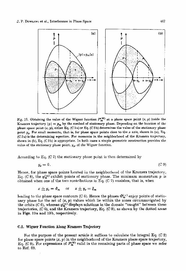
J. P. DOWLINC e t al., Interference in Phase Space 467

’ t P ’ t P

Fig. 19. Obtaining the value of the Wigner function Pkw at D phase space point (z, p) inside the Kramers trajectory Jpl = p, by the method of stationary phase. Depending on the location of the phase space point (z, p ) , either Eq. (C 3a) or Eq. (C 3 b) determines the value of the stationary phase point yr For small momenta, that is, for phase space points close to the x axis, shown in (a), Eq. (C 38) is the determining equation. For momenta in the neighborhood of the Kramers trajectory, shown in (b), Eq. (C3b) is appropriate. I n both cases a simple geometric construction provides the value of the stationary phase point, y8, of the Wigner function.

According to Eq. (C 7) the stationary phase point is then determined by

y s = 0. (C 9)

Hence, for phase space points located in the neighborhood of the Kramers trajectory, Eq. (C 8), the &*I exhibit points of stationary phase. The minimum momentum p is obtained when one of the two contributions in Eq. (C 7) vanishes, that is, when

x&yy,=.9., or x f ~ s = t m

leading to the phase space contours (C 6). Hence the phases @h+) enjoy points of stationary phase for the set of ( x , p ) values which lie within the zones circumnavigated by the orbits (C 6), whereas &=*) displays solutions in the domain “caught” between these trajectories, (C 6), and the Kramers trajectory, Eq. (C 8), as shown by the dotted areas in Figs. 19a and 19b, respectively.

C.2. Wigner Function Along Kramers Trajectory

For the purpose of the present article it suffices to calculate the integral Eq. (C 2) for phase space points (2, p ) in the neighborhood of the Kramers phase space trajectory, Eq. (C 8). For expressions of P’,W valid in the remaining parts of phase space we refer to Ref. 69.


According to Eq. (C 9) the stationary phase point is determined by yI = 0. A straight- forward way to find Pkw) consists of expanding g&*) around y = 0, that is

From Eq. (C 3b) we find

and

(C l l a )

(C 11 b)

With the help of Eqs. (C 2c), (C 3b), and (C 11), we arrive a t

which reduces Eq. (C 10) to

~ ~ * ’ ( z ; Y ) = 2 ( P , r t ~ ) 2 / + ~ ~ 1 / + 1 d2P, 3 .... (C 1 2 )

The quantity denotes the curvature of the Kramers phase space trnject,ory Eq.

(2.2 b ) in the upper half plane ( p > 0) of phase space. When we awun~e R potential U(I) = U(’)(z) with a single minimum at the origin, the Kramers phase space trajectory, Eq. (2.2b), has negative curvature, that is,

d X 2

and Eq. (C 12) reads

p:$)(x; y ) = 2(p , f p ) y -+ The Wigner function, Eq. (C 2 a) then simplifies to

Here we have made use of the definition of the normalizat,ion constant Mm, given by Eq. (2.2e), as well as the Heaviside step function 8 = 8(p) . Moreover, we have evaluated the slowly varying contribution

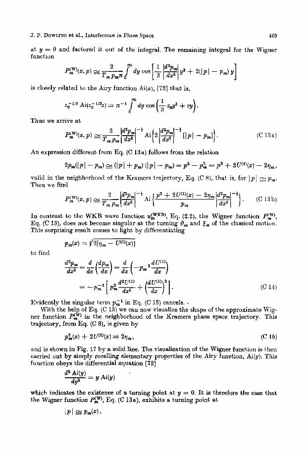
J. P. DOWLIXQ et al., Interference in Phase Space

at y = 0 and factored it out of the integral. The remaining integral for function

is closely related to the Airy function Ai(x), [72] that is,

Thus we arrive at

469

the Wigner

(C 13a)

An expression different from Eq. (C 13a) follows from t h e relation

2Pm(lPl - p m ) E ( ( P I + P m ) ( I P J - Pm) = p a - = pa + ~ u " ) ( x ) - 2 v m ,

valid in the neighborhood of the Kramers trajectory, Eq. (C 8), that is, for Ipl z p m . Then we find

In contrast to the WKB wave €unction uLwKB), Eq. ( 2 . 2 ) , the Wigner function PLw), Eq. (C 13), does not become singular a t the turning tIlm and Em of the clnssicnl motiun. This surprising result conies to light by differentiating

Pm(x) = I'2[qm - u(~)(x)I to find

(C 14)

Evidently the singular term p;' in Eq. (C 13) cancels. . With the help of Eq. (C 13) we can now visualize the shape of the approximate Wig-

ner function Frnw in the neighborhood of the Kramers phase space trajectory. This trajectory, from Eq. (C S), is given by

p $ ( x ) + 2U(')(S) = 2qm, (C 15)

and is shown in Fig. 17 by a solid line. The visualization of the Wigner function is then carried out by simply recalling elementary properties of the Airy function, Ai(y). This function obeys the differential equation [ 7 2 ]

which indicates the existence of a turning point a t y = 0. It is therefore the case that the Wigner function pmm, Eq. (C 13a), exhibits a turning point a t

IP I E P m k ) 2


that is, along the Kraniers orbit, Eqs. (C 8) and (C 16). For positive arguments the Airy function decays [72]; as a result the phase space distribution PAW decays for lpl > pm, that is, for phase space points that lie outside of the Kramers trajectory, as indicated in Fig. 17. Moreover, Eq. (C 13b) suggests that P!z) enjoys a maximum of positive value along the phase space contour line following from Eq. (C 13a), in terms of momenta, as

and from Eq. (C 13b) in terms of energies, as

(C 16a)

(C 16b)

Here we have approximated [72] the location of the first maximum of the Airy function Ai = Ai(y) by y = - 1. These expressions are identical in the limit of lp I p,, that is, for phase space points close to the Kramers orbit, Eqs. (C 8) or (C 15).

The approximations, Eq. (C 13), bring also to light the central argument for rejecting a true probability interpretation of the Wigner phase space density : The Airy function and hence, via Kq. (C 13), P&w can assume negative values. The first zero of Ai = Ai(y) occurs [78] around y = -2, that is, along the phase space contour line following either

or from Eq. (C 13 b)

(C 17a)

(C 17 b)

For phase space points (2, p ) that lie inside the Kramers-circumnavigated phase space domain, PAw) can alternate between positive and negative values. Hence, PAw) consists o f phase space waves with wave crests and troughs, as exemplified in Fig. 36 for the harmonic oscillator. Only the last M‘igner crest, located at the Kramers orbit, has d- ways positive values.

I n the most elementary version, we can replace this Wigner crest by a “moclrup” Wigner toroid of an approsimate height given by the maximum of Pk‘, along the phase space trajectory Eq. (C 16), that is,

1 2

Here we have introduced the approximation 1721 Ai(-1) G - . The Wigner toroid

intersects the x-p oscillator phase space plane and provides the two phase space curves given by the Kramers orbit of energy rim, Eq. (C 15), and the first zero of the Wigner function, Eq. (C 17), corresponding to the energy yip). This band - the base or “foun- dation” of the toroid - is analogous to the mth Planck-Bohr-Sommerfeld band of Sec. 3. It has a width in momentum, given by Eq. (C 17a)

The weighted area of phase space taken up by this Wigner toroid reads then

JJ base of Wiener toroid

dx d p I @ ) ( X ) = 2 J d x ApLW(x) hkm(~)

= T,‘ 2 J dxlp i ’ (2) = TG1 9 dt = 1 (C 20)

J. P. DOWLIXU et al., Interference in Phase Space 471

t h a t is, it approximately covers a phase space domain equal to unity. Here we have made use of Eqs. (C 18) and (C 19) and the definition of the period of the mth orbit, Eq.

We gain deeper insight into the physical content of this Wigner crest by investiga- (2.2f).

ting to what extent the remarkable property 00

.24 = J (12, p',")(., P) 2

- W

valid fur any Wigner function, holcls true for the approximate Wigner function, Eq. (C 13). When we restrict the integration over the momentum p only to the neighborhood of the two thin slices cut out of the Wigner toroid, shown in Fig. 17, we find

Hence the classical probability Wg!; of finding a particle at position x is related to the toroid given by Eqs. (C 18) and (C 19), or in its more precise form, to the Wigner crest of Eq. (C t3). The rapid oscillations of the probability u i , reflecting the interference of the counter propagating waves, are however missing in this picture. They are contained in the wave crests and troughs in the phase space domain surrounded by the Wigner crest, alluded to already by the oscillations of the Airy functions. The precise form of these oscillations, however, we can only derive by making use of the stationary phase points of @$), given by Eq. (C 3a). For a detailed discussion of this point see Ref. 69. We are therefore led to the most elementary approximation of P:'), valid in the absence of interference phenomena [82]: A deltn function located along the Kramers orbit.

We conclude this section by noting that when we integrate Eq. (C 21) over position we arrive a t Eq. (C 20). Moreover, we emphasize that the classical probability Wg!',, Eq. (C 21), is singular a t the turning points 8m and tm, whereas the Wigner function approximation, Eq. (C 13), is not.

C.3. Wignor Crest of Harmonic Oscillator Versus Planck-Bohr-Sommcrleld Band

We conclude this appendix by applying the results of Appendix C. 2. to the example of a harmonic oscillator potential U(')(X) = 2212. I n this case the exact Wigner function for the mth energy eigenstate reads [55 , 56, 701

where L, denotes the mth Laguerre polynomial. The two phase space orbits Eq. (C 6) separating the domains where ~ 2 ) or @g) enjoy stationary phase points, simplify to

that is, to two circles located at x = f5,/2. The radius of each circle is half of that of the Kramers phase space trajectory

p2 + (z & 5m/2)' = ( tm/2) ' ,

We now derive the toroid approximation, Eq. (C 13), for a harmonic oscillator potential. With the help of Eq. (C 14), that is,

(C 23) d2pm - - 2qm - - 2(m. + 1/2)

P i 3 ax2 P m


and the relation Tm = 2n, we find for Eq. (C 13a),

(C 24a)

and for Eq. (C 13 b), PAW(., p ) 7r1[2(m + 1/2)]-* Ai{[2(m + 1/2)]-* [22 + p 2 - 2(m + 1/2)]). (C 24b)

The radii of the circular contour lines of the maximum and of the largest zero of the Wigner wave crest, that is, the radius of the center line rg), and that of the inner edge of the toroid rF), follow immediately from Eqs. (C 16a), (C 17a), and (C 23) ‘when we set x = 0,

(C 25a) 1 rg)= I p(mmax)(x = 0) I = [2(m + 1/2)]* - [2(m + 1/2)]-*

and

r 2 ) = I p y ) ( x = 0) ) = [2(m + 1/2)]1 - [2(m + 1/2)]-*. (C 25b) We emphasize that this is quite different from the corresponding expressions [2(m + 1/2)]1’2 and (2m)’I2 for the Planck-Bohr-Sommerfeld band, following from Nqs. (3.1) and (3.2a). The radial width of the Wigner toroid, Arkw), and its height hkm follow then from Eqs. (C 18), (C 22), (C 23), (C 24), and (C 25b), and read

(C 26a) drc,W,zz r, - re) = [2(m + 1/2)]-i and

hkW = (2n)-l [2(m + 1/2)]-*. (C 26b) When we compare and contrast these expressions to the corresponding ones of the nit h Planck-Bohr-Somnierfefeld band

ArEBS’ = [2(nt + l)]’ - (2rn)t 2 [2(m + 1 / 2 ) ] 4 (C 27a)

h p s ) = (274-1 (C 27b) we find the Wigner toroid to be broader than the band, as indicated in Fig. 16. Its peak- height is correspondingly smaller as to normalize the phase space area. For the Wigner crest we find from Eqs. (C 25a) and Eq. (C 26)

and

and for the corresponding expressions of the Planck-Bohr-Sommerfeld band

2n r,,, . drgBs) - h g B S ) = [2(m + 1/2)]112 [2(m + 1/2)]-’’~ = 1,

following from Eq. (C 27), and as summarized in Table 2.

Bppendix D. Band Overlap versus Crest Intersection

In this appendix we parameterize the x-p oscillator phase space in the neighborhood of the railway switch between the mth and the nth Kramers phase space orbits, shown in Fig. lob, defined by

PA%) = P&J (D 1)

J. P. DOWIJNG et al., Interference in Phase Space li3

via the energies

and

corresponding to the classical niotions in the two potentials U(I) and V2). This allows us to rederive the area of crossover between the two Planck-Bohr-Sommerfelcl bands

which in Appendix B we have calculated with the help of Bohr's correspondence principle. Moreover, it enables us to evaluate t h e phase space overlap ALW; between two Airy-function-type Wigner crests determining the classical jump probability.

The phase space element, of area, d x dp , is then related to the area element dr)(') d7f2) via t,he relation [83]

d x dP = 1/911922 - 912 2 d 17 (1) d 7 p (D 3) where the metric coefficients gii are defined by the Jacobian matrix elements

ax ax ap a p 912 = 921 = arlc',ar1(2) f al.lcl,a77(2).

For the evaluation of the matrix coefficients gii, Eq. (D 4), i t is necessary to express the original phase space variables x and p in terms of the new variables and q(?). For arbitrary potentials U ( l ) and U(2) this cannot be performed in closed forni. In the neighborhood of xc, however, we may expand the potential U(') around L, and subtract

and add, in Eq. (D 2 a), the kinetic energy of the mth orbit a t the crossing point p i ( x c ) . When this is clone we arrive at

1 2

1 1 2 a Pi(.,, + 77m + -&- (z - 5 e ) - (D 5) u(i)lz-zc +1) g - p2 - -

Here

(D 6) 1 2 q m = - P i @ ) + U(l)(X)

denotes the total energy of the mth orbit. Differentiation of Eq. (D 6) with respect to x leads to the relation

which when substituted into Eq. (D 5) yields


In the remainder of this appendix the momenta pm and pn and their derivatives are presumed to be evaluated at 2,. The same procedure as used above, but starting instead from E(1. (D 2b), establishes the relation

where

denotes the total energy on the nth orbit in potential U(2) . When we subtract Eq. (D 7b) from (D 7a) and make use of the equality of momenta a t the crossing point, Eq. (D l), we arrive (after some algebra) a t

Addition of Eqs. (D 7a) and (D 7b) provides

7") + q(2) = P' - P: + rlm + rln - P ~ ( P L + P;) (z - zc)

p2 - P: = (P + Pn) (P - Pn)

(D 9) where we have again made use of Eq. (D 1). In the neighborhood of the orbit crossing, the properly

2pn * (P - Pn) holds true, which together with Eq. (D 8) reduces Eq. (D 9) to

When we substitute t'hese expressions int'o Eqs. (D 4a), (D 4b), and (D 4c), we find

and

and finally

Here we have repeatedly made use of Eq. (D l), that is, of the equality of momenta a t the crossing point implicitly defined by pm(xc) = p,,(x,). With the help of these expressions the phase space area element, Eq. (D 3), reads

To test this result, we now rederive the area of cross-over, AKF), between the mth and the nth Plancli-Bohr-Sommerfeld band, found in Appendix B. Moreover, we calculate the area in phase space, A$$, taken up by the crossing of the two corresponding Wigner crests. In both cases [k (PBS, W ) ] this crossover consists of the two symmetrically located zones, as show in Fig. 4, yielding the total area


According to Fig. 12 in Sec. 3, the edges of the mth and nth Plaiick-Bohr-Sommerfeld bands are given in terms of the reduced actions fl) and f 2 ) , that is, by m and m + 1 or n and n + 1, respectively. Hence, for the evaluation of AEZs) i t is more convenient to introduce as integration variables y(') and f 2 ) , rather than the energies 77''' and r f ) , giving

m + l n f l a p a p Bgy = 2 [ p mpn I PA - PA I I-' J d f ' ) j d f " v) v) *

-- - (2n)-1$ dzp-l(x; f " ) ) = (2n)-l T ( f ( j ) ) ,

m n

When we recall Eq. (B 2), a$ (7)

a,,") we can perform the integrals by evaluating the periods at the average actions $(I) =

m + - and f z ) = n + T , that is, 1 1 2

T l / ( i ) = m + * T m and T~Y(ZL,,++ = Tn which yields

AKZS) = 2(2n12 [Tmpm(zc) Tnpn(~c)I-' l ~ A ( z c ) - ~L(xc)l-',

in agreement with Appendix B. I n the case of the Wigner crests, we keep q(l) and qt2) as the integrat,ion variables.

According to Appendix C, each crest is built out of phase space trajectories corresponding to energies @). These energies range approximately from q p ) to qm, where according to Eq. (C 17b)

(D 13a)

determines the largest zero of Pkw, and qm is the energy of the Kramers orbit. Similarly, the energy rf2) for the crest of Phm varies between

(D 13 b)

,,fzp) = mm - pm(xc) l ~ k ( ~ c ) I*

@d = qn - ~ n ( z c ) l~A'(zc) I* and qn. With these limits of integration, Eq. (D 12) reduces to

(zero)] A(w, = 2 [ ~ n , - 7L"'I [qs - qn Pm(sc) Pn(sc) l ~ k ( ~ c ) - A ( % c ) I m.n

and with the help of Eq. (D 13) we find p(rc) d2Pn(z.))* -q?! = 2 IPk(4 - P;(%)I-l -- dx2 d 3 .

References

[l] PLANCK, M.: Ann. Phys. (Leipzig) 60 (1916) 385. [2] HERZBERO, G.: Molecular Spectra and Molecular Structure, Vol. I, Spectra of Diatomic Mole-

[3] SCHBODINGEH, E.: Ann. Phys. (Leipzig) 79 (1926) 361; 79 (1926) 489. [4] BORN, M.; OPPENEEIMER, R.: Ann. Phys. (Leipzig) 84 (1927) 457. [5] EBBENFEST, P. : Ann. Phys. (Leipzig) 61 (1916) 327. [6] BORN, M.: Atommechanik, In: "Struktur der Materie in Einzeldarstellungen" (M. Born and

[7] BOER, N.: Collected Works (L. Rosenfeld, ed.). Amsterdam: North-Holland 1976; SOMMERFELD,

[8] SCHOPS, H. G.: Ann. Phys. (Leipzig) 45 (1988) 696.

cules. Princeton: von Nostrand 1965.

J. Franck, eds.). Berlin: Springer 1925.

A.: Sitzungsber. der kgl. Bayr. Akad. d. Wiss. (1915) 425; ibid. (1915) 459.

47G Ann. Physik Leipzig 48 (1991) 7

[9] SOMMERFELD, A.: Ann. Phys. (Leipzig) 61 (1916) 1. [lo] KRUSKAL, M.: In: “Conference on Mathematical Models in the Physical Sciences” (S. Drobot

[ l l ] WESTZEL, G.: Z. Phys. 38 (1926) 518. [12] KRAXERS, H. A.: Z. Phys. 30 (1926) 829. [13] BRIILOUIN, L.: C. R. Acad. Sci. (Paris) 183 (19%) 24. [11] DEBYE, P.: Phys. Z. 58 (199) 170. [15] DARWKX. C. G.: Proc. R. SOC. London, Ser. 117 A (1927) 258. [16] PAUL[. W. : Die allgemeinen Prinzipien der Wellenmechanik, In: “Handbuch der Physik”.

Eli] KRAXERS, H. A., Quantentheorie des Elektrons und der Strahlung, Vol. 2: In: “Hand- und

[18] BERRY, M. V.; MOUNT, K. E.: Rep. Prog. Phys. 35 (1972) 315. [I91 LIBOFF, R. L.: Int. J. Theor. Phys. 18 (1979) 185; Phys. Today 37 (Feb., 1981) 50. [20] WHEELER, J. A.: In: “Studies in Mathematical Physics” (E. H. Lieb, B. Simon, and .LS. Wight-

[21] WHEELER, J. A.: Lett. Math. Phys. 10 (1985) 201. [22] HLLL, D. L.; WHEELER, J. A,: Phys. Rev. 89 (1953) 1102. [23] WALLS, D. F.: Nature (London) 306 (1983) 141; ibid. 324 (1986) 210. [24] SCIILEICH, W. P.; WHEELER, J. A.: Nature (London) 306 (1987) 574; J. Opt. SOC. Am. B4

(1987) 1715. [25] SCHEXZLE. A.; BREWER, R. G.: Phys. Rev. A (1986) 3127; and in: “Lecture Notes in Physics”,

Vol. 28s (F. Ehlotzky, 4.). Berlin: Springer-Verlag 1987. [26] BOH~I, D. : Quantum Theory. Englewood: Prentice-Hall 1951. 1271 FRANCK, J.: Trans. Faraday SOC. 31 (1925) 536. [B] CONDON, E. U.: Phys. Rev. 58 (1926) 1182; ibid. 35 (1928) 858; Am. J. Phys. 15 (194i) 3 6 . [29] CONDON, E. U.: In: “Handbook of Physics” (E. U. Condon and H. Odishaw eds.). New York:

[30] MULLIKEN, R. S.: J. Chem. Phys. 56 (1951) 309. [31] SCHLEICH, W. P.; WALTHER, H.; WHEELER, J. A.: Found. Phys. 18 (1988) 953. [32] SCHLEICH, W. P. ; WALLS, D. F. ; WHEELER, J. A.: Phys. Rev. A 38 (1988) 1177. [33] CLYNE, M. A. A.; M c D m m , I. S.: J. Chem. SOC. Faraday Trans. II,78 (1976) 2242. [34] BROWN, W. G.: Z. Phys. 89 (1933) 768. [Xi] DEXTBODER, W.: Laser Spectroscopy. Berlin: Springer 1981; SLANOEE, T. G.; JUSINSKI. L. E.;

BLACK. G. ; GADD, G. E. : Science 241 (1988) 945. [36] TRAUTMANN, M. : Dynamik selektierter Quantenzustiinde an zwei Beispielen, (LudwigMaxi-

milians-Universitlt Miinchen, Doktorarbeit 1984) ; published as Max-Planck-Institut f i i r Quan- tenoptik Report MPQ 90 (1984).

and P. A. Viebrock, eds.). Prentice Hall: Englewood Cliffs 1963.

Vol. 24 (H. Geiger and K. Scheel, eds.). Berlin: Springer 1933.

Jahrbuch der Chemischen Physik”. Leipzig: Eucken-Wolf 1938.

mm, eds.). Princeton: Princeton University h e s s 197G.

McGraw-Hill 1967.

[37] TRAUTMANN, M.; WANNER, J. ; ZHOU, S. K.; VIDAL, C. R.: J. Chem. Phys. S2 (1985) 693. [38] CHILD, M. S.: Molecular Collision Theory. London: Academic Preess 1974; also in: “Semiclassical

Methods in Molecular Scattering and Spectroscopy” (M. S. Child, ed.). Dordrecht: D. Reidel 1979.

[39] WHEELER, J. A; ZUREK, W. H.: Quantum Theory and Jfeasurement. Princeton: Princeton University Press, 1983.

[40] FEYNXAX, R. P.; HIBBS, A. R.: Quantum Mechanics and Path Integrals. New York: McGraw- Hi11 1965.

[41] SCHULMAN, L. S.: Techniques and Applications of Path Integration. New York: J. Wiley 1981. [42] BUTCHISSON, E.: Phys. Rev. 36 (1930) 410. [43] BERGMIANN, E. E. : Nuovo Cimento 22 (1974) 249. [14] FRIEDMANIT, B. : Lectures on Applications-Oriented Mathematics. Son Francisco : Holden Day

[15] NELLER, E. J.: J. Chem. Phys. 67 (1977) 3339. 1969.

J. P. D o w ~ r i a et al., Interference in Phase Space 477

[46] JAHNKE, E.; EMDE, F.: Tables of Functions. New York: Dover 1945. [47] HECHT, E.; ZAJAC, A.: Optics. Reading: Addison-Wesley 1980. [48] FEYNMAN, R. P. ; WHEELER, J. A. : (unpublished). [49] WIIEELER, J. A.: Phys. Today 42 (February 1989) 24. [50] WHEELER, J. A.: J. Opt. SOC. Am. 87 (1947) 813. [5l] SLATER, J. C.: Quantum Theory of Atomic Structure. New York: McGraw-Hill 1960. [XI PLANCK, M.: Vorlesungen iiber die Theorie der Wiirmestrahlung. Leipzig: J. A. Barth 19OG. [53] WIGNER, E. P.: Phys. Rev. 40 (1932) 749. [54] STENHOLM, S.: Euro. J. Phys. 1 (1980) 244. [.is] TATARSKII, V. I.: Usp. Fiz. Nauk. 139 (1983) 587 [Sov. Phys. Usp. 26 (1983) 311; BALAZS, N. L.;

[56] HILLERY, M.; O’CONNELL, R. F.; S o m y , M. 0.; WIGNER, E. P.: Phys. Rev. 106 (1984) 121. [57] O’CONNELL, R. F.; WIQNER, E. P.: Phys. Lett. 83 A (1981) 145; O’CONNELL, R. F.; RAJA-

QOPAL, A. K.: Phys. Rev. Lett. 48 (1982) 525; O’CONXELL, R. F.; WALLS, D. F.: Nature (Lon- don) 312 (1984) 257; WODKIEWCZ, K.: Phys. Rev. Lett. 52 (1984) 1046.

[58] HELLER, E. J.: J. Chem. Phys. 68 (1978) 2066; LEE, H.-W.; SCULLY, M. 0.: J. Chem. Phys. 77 (1982) 4604.

[59] WOOD, R. W.: Physical Optics. New York: Macmillan, 1st ed. 1911, and 3rd ed. 1931, reprinted in Woodbury: Optical Society of America 1990.

[GO] LANDAU, L. D.: Z. Sowjet. 1 (1932) 88; reprinted in TER HAAR, D.: Collected Papers of L. D. Landau. Oxford: Pergamon 1965; LANDAU, L. D.; LIFSHITZ, E. M.: Quantum Mechanics - Nonrelativistic Theory. Oxford: Pergamon 1958.

[61] JABLONSKI, A.: Phys. Rev. 68 (1945) 78. [62] ROJAS, D. H.; KRVGER, H.: J. Phys. B 19 (1986) 1553. [63] TELLINGHUISEN, J.: Phys. Rev. Lett. 34 (1975) 1137; also in: “Advances in Chemical Physics”,

[64] HEW, T. A. ; TRAUTMANN, D.; BAUR, G.: J. Phys. B 29 (1989) 727. [65] CHESTER, C.; FRIEDMANN, B.; URSELL, F.: Proc. Cambridge Philos. SOC. 53 (1957) 599; BLEI-

STEIN, N. ; HANDELSMANN, R. A. : Asymptotic Expansions of Integrals. New York: Holt, Rine- hart, and Winston 1975.

JENNINGS, B. K.: Phys. Rev. 104 (1984) 347.

Vol. LX (I. Prigogine and S. A. Rice, eds.). Chichester: Wiley 1985.

[66] FRANK, P.; GLASER, W.: Z. Phys. 61 (1930) 640; GLASW, W.: Z. Phys. 61 (1930) 644. [67] BALAZS, N. L.; ZIPPEL, G. G.: Ann. Phys. (NY) 77 (1973) 139. [68] BERRY, M. V.; BALAZS, N. L.: J. Phys. A 12 (1979) 625. [69] BERRY, M. V.: Phil. Trans. R. SOC. London, Ser. 28’7 A (1977) 237; Proc. R. SOC. London, Ser.

[70] KLAUDER, J. R.: Bell Syst. Tech. J. 39 (1960) 809. [71] SZEQO, G.: Orthogonal Polynomials. New York: American Mathematical Society 1939. [72] ABRAMOWITZ, M.; STEQUN, I. E.: Handbook of Mathematical Functions. Washington: National

[73] COHEB, L.: In: “Frontiers of Nonequilibrium Statistical Physics” (G. Moore and M. 0. Scully,

[74] MILBURN, G. J.; WALLS, D. F.: Phys. Rev. A 38 (1988) 1087; MILBURN, G. J.: In: “Nonclassical

[75] VOGEL, K.; SCHLEICH, W. P. : in: “Fundamental Systems in Quantum Optics” (J. Daliberd,

[76] SANDERS, B.: Phys. Rev. A 39 (1989) 4284. [77] Krar, M. S.; DE OLIVEIRA, F. A. M.; KNIGHT, P. L.: Phys. Rev. A 40 (1989) 2494; DE OLIVEIRA,

F. A. M.; Kw, M. S.; KNIGHT, P. L.; B ~ E K , V.: Phys. Rev. A41 (1990) 2645; OLIVEII~A, F. A, M.; KNIGHT, P. L.; PALDU, G. M.; EKEBT, A.: in: “Noise and Chaos in Nonlinear Dyna- mica1 Systems,” (F. Moss, L. Lugiato, and W. Schleich, eds.). Cambridge: Cambridge Press 1990.

423 A (1989) 219; ibid 424 (1989) 279.

Bureau of Standards 1957.

eds.). New York: Plenum Press 1986; Proc. IEEE 77 (1989) 941.

and Squeezed Light” (P. Tombesi and R. Pike, eds.). New York: Plenum Press 1988.

J. M. Raimond, J. Zinn Justin, eds.). Amsterdam: Elsevier 1991.


[78] CAVES, C. M.; ZHU, C. ; NILBURN, G. J. ; SCHLEICH, W. P. : Phys. Rev. A 43 (1991) 3864. [ is] SCIILEICH, W. P.; HOROWCZ, R. J.; VARRO, S.: Phys. Rev. A 40 (1989) 7405; see also In:

“Quantum Optics, Vol. V” (D. F. Walls and J. Harvey, eds.). Heidelberg: Springer 1989; SCHLEICH, W. P.; DOWWNG, J. P.; HOROWICZ, R. J.; VARRO, S.: In: “New Frontiers in Qnun- turn Electrodynamics and Quantum Optics” (A. 0. Barut, ed.). New York: Plenum Press 1990.

[SO] FLEISCKHAUER, M.; SCHLEICH, W. P.: Phys. Rev. A (submitted for publication). [81] GRADSTEYN, I. S.; RYZHIK, I. M.: Table of Integrals, Series and Products. New York: Aca-

demic Press 1980. [82] D a m , J. P.: In: “Energy Storage and Redistribution in Molecules” (J. Hinze, ed.). Kew York:

Plenum Press 1983; and in: “Semiclassical Descriptions of Atomic and Nuclear Collisions” (J. Bang and J. de Boer, eds.) Amsterdam: Elsevier 1985.

[83] TEICEMANN, H. : Physikalische Anwendungen der Vektor- und Tensorrechnung. Mannheirn : Bibliographisches Institut: 1973.

Bei der Redaktion eingegangen am 1. Februar 1991.

Anschr. d. Verf.: Dr. J. P. DOWLIXI US Army Missile Command

Redstone Arsenal, AL 3.398, USA

Prof. W. P. SCHLEICH Abteilung fur Theoretische Physik I11 Universitiit Ulm Oberer Eselsberg W - 7900 Ulm, Deutschland and Center for Advanced Studies, Department of Physics and Astronomy, University of New Mexico, Albuquerque, NM 87131, USA

Prof. J. A. WHEELER Department of Physics, Princeton University, usual location, Princeton, N J 08544, USA and Department of Physics, University of Texas at Austin, Austin, TX 78712, USA

AiiSMI-RD-WS

Download - ANNALEN DER PHYSIK - LSUjdowling/publications/Dowling91.pdf · ANNALEN DER PHYSIK 7. Folge. Band 48. 1991. Heft 7, S. 423-502 Interference in Phase Space ... In the semiclassical

Top Related