Download - Analytic Geometry - Gordon Fuller
ANALYTIC GEOMETRY
(10RDOX FULLER
Professor of Mathematics
Texas Technological College
1954
ADDISON-WESLEY PUBLISHING COMPANY, INC.
CAMBRIDGE 42, MASS.

Copi/right 1954
ADDISON-WESLEY PUBLISHING COMPANY, Inc.
Printed in the United States of America
ALL RIGHTS RESERVED. THIS BOOK, OR PARTS THERE-
OF, MAY NOT BE REPRODUCED IN ANY FORM WITHOUT
WRITTEN PERMISSION OF THE PUBLISHERS.
Library of Congress Catalog No. 54-5724
ANALYTIC GEOMETRY
ADDISON-WESLEY MATHEMATICS SERIES
ERIC REISSNER, Consulting Editor
Bardell and Spitzbart COLLEGE ALGEBRA
Dadourian PLANE TRIGONOMETRY
Davis MODERN COLLEGE GEOMETRY*
Davis THE TEACHING OF MATHEMATICS
Fuller ANALYTIC GEOMETRY
Gnedenko and Kolmogorov LIMIT DISTRIBUTIONS FOR SUMS OF INDEPENDENT
RANDOM VARIABLES
Kaplan ADVANCED CALCULUS
Kaplan A FIRST COURSE IN FUNCTJJONS OF A COMPLEX VARIABLE
Mesewe FUNDAMENTAL CONCEPTS OF ALGEBRA
Munroe- INTRODUCTION TO MEASURE AND INTEGRATION
Perlis THEORY OF MATRICES
Stabler AN INTRODUCTION TO MATHEMATICAL THOUGHT
Struik DIFFERENTIAL GEOMETRY
Struik ELEMENTARY ANALYTIC AND PROTECTIVE GEOMETRY
Thomas CALCULUS
Thomas CALCULUS AND ANALYTIC GEOMETRY
Wade THE ALGEBRA OF VECTORS AND MATRICES
Wilkes, Wheeler, and Gill THE PREPARATION OF PROGRAMS FOR AN ELECTRONIC
DIGITAL COMPUTER
PREFACE
In recent years there has been a marked tendency in college mathe-
matics programs toward an earlier and more intensive use of the methods
of calculus. This change is made in response to the fact that college
students are faced with more and more applications of mathematics in
engineering, physics, chemistry, and other fields. There is a pressing need
for a working knowledge of calculus as early as possible. Consequently
many teachers are making a close scrutiny of the traditional topics of
freshman mathematics. This is done in an effort to determine the ma-
terial and emphasis which will lay the best foundation for the study of
calculus.
In the light of present needs, this analytic geometry is planned primarily
as a preparation for calculus. With this end in mind, a few of the usual
topics are not included and certain others are treated with brevity. Theomitted material, consisting of an appreciable amount of the geometry of
circles and a number of minor items, is not essential to the study of calculus.
The time saved by cutting traditional material provides opportunity for
emphasizing the necessary basic principles and for introducing new con-
cepts which point more directly toward the calculus.
Students come to analytic geometry with a rather limited experience in
graphing. Principally they have dealt with the graphs of linear and cer-
tain quadratic equations. Hence it seenis well to let this be the starting
point. Accordingly, the first chapter deals with functions and graphs.
In order that this part shall go beyond a review of old material, the ideas
of intercepts, symmetry, excluded values, and asymptotes are considered.
Most students in algebra are told (without proof) that the graph of a
linear equation in two variables is a straight line. Taking cognizance of
this situation, it appears logical to prove directly from the equation that
the graph of A x + By + C = is a straight line. Having established this
fact, the equation can be altered in a straightforward procedure to yield
various special forms. The normal form, however, receives only incidental
mention.
The transformation of coordinates concept is introduced preceding a
systematic study of conies. Taken early or late in the course, this is a
difficult idea for the students. By its early use, however, the students
may see that a general second degree equation can be reduced to a simple
form. Thus there is established a logical basis for investigating conies bymeans of the simple equations.
Although employing simple forms, the second degree equation is intro-
duced at variance with the traditional procedure. As with the linear

VI PREFACE
equation, it seems logical to build on the previous instruction given to the
students. In algebra they have drawn graphs of conies. The words
circle, parabola, ellipse, and hyperbola are familiar to many of them. In
fact, some students can classify the type of conic if the equation has no xyterm. Tying in with this state of preparation, the conic may jiaturally
and logically be defined analytically rather than as the locus of a moving
point. The equations then lend themselves to the establishment of various
geometric properties.
In harmony with the idea of laying a foundation for calculus, a chapter
is given to the use of the derivatives of polynomials and of negative integral
powers of a variable. Applications are made in constructing graphs, and
some maxima and minima problems of a practical nature are considered.
The chapter on curve fitting applies the method of least squares in
fitting a straight line to empirical data.
Many students come to calculus with little understanding of polar coor-
dinates, therefore polar coordinates are discussed quite fully, and there is
an abundance of problems.
The elements of solid analytic geometry are treated in two concluding
chapters. The first of these takes up quadric surfaces and the second deals
with planes and lines. This order is chosen because a class which takes
only one of the two chapters should preferably study the space illustrations
of second degree equations. Vectors are introduced and applied in the
study of planes and lines. This study is facilitated, of course, by the use
of vectors, and a further advantage is gained by giving the students a
brief encounter with this valuable concept.
The six numerical tables provided in the Appendix, though brief, are
fully adequate to meet the needs which arise in the problems.
Answers to odd-numbered problems are bound in the book. All of the
answers are available in pamphlet form to teachers.
The book is written for a course of three semester hours. While an
exceptionally well prepared group of students will be able to cover the
entire book in a course of this length, there will be excess material for
many classes. It is suggested that omissions may be made from Chapters7 and 8, Sections 6-7, 9-8, 12-7, and 12-8.
The author is indebted to Professor B. H. Gere, Hamilton College,
Professor Morris Kline, New York University, and Professor Eric Reissner,
Massachusetts Institute of Technology. Each of these men read the
manuscript at various stages of its development and made numerous
helpful suggestions for improvement.
G. F.
January, 1954
CONTENTS
CHAPTER 1. FUNCTIONS AND GRAPHS 1
1-1 Introduction 1
1-2 Rectangular coordinates 1
1-3 Variables and functions 3
1-4 Useful notation for functions 4
1-5 Graph of an equation 5
1-6 Aids in graphing 6
/'TT/The graph of an equation in factored form 10
^1-8 Intersections of graphs 11
1-9 Asymptotes 13
CHAPTER 2. FUNDAMENTAL CONCEPTS AND FORMULAS 17
2-1 Directed lines and segments 17
2-2 The distance between two points 18
2-3 Inclination and slope of a line 21
2-4 Angle between two lines 24
2-5 The mid-point of a line segment 27
2-6 Analytic proofs of geometric theorems 28
CHAPTER 3. THE STRAIGHT LINE 31
3-1 Introduction 31
3-2 The locus of a first degree equation 31
3-3 Special forms of the first degree equation 32
3-4 The distance from a line to a point 37
<<35>Families of lines 40
3-6 Family of lines through the intersection of two lines 41
CHAPTER 4. TRANSFORMATION OF COORDINATES 45
4-1 Introduction 45
4-2 Translation of axes 45
4-j$ Rotation of axes 49
vj^? Simplification of second degree equations ...-- 51
CHAPTER 5. THE SECOND DEGREE EQUATION. . ^/C 56
5-1 Introduction 56
5-2 The simplified equations of conies 57
5-3 The parabola 58
5-4 The focus-directrix property of a parabola 59
5-5 The ellipse 64
5-6 The foci of an ellipse 65
5-7 The eccentricity of an ellipse 68
5-8 The hyperbola 70
5-9 The asymptotes of a hyperbola 71
5-10 Applications of conies 74
5-11 Standard forms of second degree equations 75
(tt$ The addition of ordinates 78
5-13 Identification of a conic 79
vii
Vlll CONTENTS
CHAPTER 6. THE SLOPE OF A CURVE 83
6-1 An example 83
6-2 Limits 856-3 The derivative 85
6-4 Derivative formulas 86
6-5 The use of the derivative in graphing 89
6-6 Maximum and minimum points 92
6-7 Applications 94
CHAPTER 7. TRANSCENDENTAL FUNCTIONS 98
7-1 Introduction 98
7-2 The trigonometric curves 98
7-3 The inverse trigonometric functions 101
7-4 The exponential curves 103
7-5 Logarithmic curves 104
7-6 The graph of the sum of two functions 105
CHAPTER 8. EQUATIONS OF CURVES AND CURVE FITTING 107
8-1 Equation of a given curve 107
8-2 Equation corresponding to empirical data 109
8-3 The method of least squares 110
8-4 Nonlinear fits 113
8-5 The power formula 114
8-6 The exponential and logarithmic formulas 117
CHAPTER 9. POLAR COORDINATES 120
9-1 Introduction 120
9-2 The polar coordinate system 120
9-3 Relations between rectangular and polar coordinates 121
9-4 Graphs of polar coordinate equations 124
9-5 Equations of lines and conies in polar coordinate forms 126
9-6 Aids in graphing polar coordinate equations 130
9-7 Special types of equations 133
9-8 Intersections of polar coordinate curves 138
CHAPTER 10. PARAMETRIC EQUATIONS 141
10-1 Introduction 141
10-2 Parametric equations of the circle and ellipse 142
10-3 The graph of parametric equations 143
10-4 The path of a projectile 146
10-5 The cycloid 147
CHAPTER 11. SPACE COORDINATES AND SURFACES 151
11-1 Space coordinates 151
11-2 The locus of an equation 152
11-3 Cylindrical surfaces 153
11-4 The general linear equation 15511-5 Second degree equations 15611-6 Quadric surfaces 157

CONTENTS IX
CHAPTER 12. VECTORS AND PLANES AND LINES 167
12-1 Vectors 167
12-2 Operations on vectors 168
12-3 Vectors in a rectangular coordinate plane 169
12-4 Vectors in space 172
12-5 The scalar product of two vectors 174
12-6 The equation of a plane 178
12-7 The equations of a line 181
12-8 Direction angles and direction cosines 184
APPENDIX 187
ANSWERS TO PROBLEMS 195
INDEX 202

CHAPTER 1
FUNCTIONS AND GRAPHS
1-1 Introduction. Previous to the seventeenth century, algebra and
geometry were largely distinct mathematical sciences, each having been
developed independently of the other. In 1637, however, a French mathe-
matician and philosopher, Ren6 Descartes, published his La Gtomttrie,
which introduced a device for unifying these two branches of mathematics.
The basic feature of this new process, now called analytic geometry, is the
use of a coordinate system. By means of coordinate systems algebraic
methods can be applied powerfully in the study of geometry, and perhapsof still greater importance is the advantage gained by algebra through the
pictorial representation of algebraic equations. Since the time of Descartes
analytic geometry has had a tremendous impact on the development of
mathematical knowledge. And today analytic methods enter vitally
into the diverse theoretical and practical applications of mathematics.
1-2 Rectangular coordinates. We shall describe the rectangular co-
ordinate system which the student has previously met in elementary
algebra and trigonometry. This is the most common coordinate systemand is sometimes called the rectangular Cartesian system in honor of
Descartes.
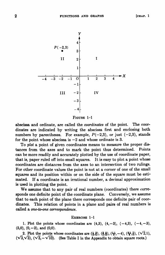
Draw two perpendicular lines meeting at (Fig. 1-1). The point
is called the origin and the lines are called the axes, OX the x-axis and OYthe ?/-axis. The x-axis is usually drawn horizontally and is frequently
referred to as the horizontal axis, and the //-axis is called the vertical axis.
The axes divide their plane into four parts called quadrants. The quad-rants are numbered I, II, III, and IV, as in Fig. 1-1. Next select anyconvenient unit of length and lay off distances from the origin along the
axes. The distances to the right along the x-axis are defined as positive
and those to the left are taken as negative. Similarly, distances upward
along the y-axis are defined as positive and those downward are called
negative.
The position of any point P in the plane may be definitely indicated by
giving its distances from the axes. The distance from the y-axis to P is
called the abscissa of the point, and the distance from the x-axis is called
the ordinate of the point. The abscissa is positive if the point is to the
right of the */-axis, and negative if the point is to the left of the g/-axis.
The ordinate is positive if the point is above the x-axis, and negative if the
point is below the x-axis. The abscissa of a point on the y-axis is zero
and the ordinate of a point on the x-axis is zero. The two distances,1
FUNCTIONS AND GRAPHS [CHAP. 1
FlGURE 1-1
abscissa and ordinate, are called the coordinates of the point. The coor-
dinates are indicated by writing the abscissa first and enclosing both
numbers by parentheses. For example, P( 2,3), or just (2,3), stands
for the point whose abscissa is 2 and whose ordinate is 3.
To plot a point of given coordinates means to measure the proper dis-
tances from the axes and to mark the point thus determined. Points
can be more readily and accurately plotted by the use of coordinate paper,
that is, paper ruled off into small squares. It is easy to plot a point whose
coordinates are distances from the axes to an intersection of two rulings.
For other coordinate values the point is not at a corner of one of the small
squares and its position within or on the side of the square must be esti-
mated. If a coordinate is an irrational number, a decimal approximationis used in plotting the point.
We assume that to any pair of real numbers (coordinates) there corre-
sponds one definite point of the coordinate plane. Conversely, we assume
that to each point of the plane there corresponds one definite pair of coor-
dinates. This relation of points in a plane and pairs of real numbers is
called a one-to-one correspondence.
EXERCISE 1-1
1. Plot the points whose coordinates are (4,3), (4, 3), (4,3), (4, 3),
(5,0), (0, -2), and (0,0).
2. Plot the points whose coordinates are (J,), (if), (V,-*), ftS), (^2,1),
(\/3,V3), (V5,-\/I6). (See Table I in the Appendix to obtain square roots.)
1-3] VARIABLES AND FUNCTIONS 3
3. Draw the triangles whose vertices are (a) (2,-l), (0,4), (5,1); (b) (2, -3),
(4,4), (-2,3).
4. In which quadrant does a point lie if (a) both coordinates are positive,
(b) both are negative?
5. Where may a point lie if (a) its ordinate is zero, (b) its abscissa is zero?
6. What points have their abscissas equal to 2? For what points are the
ordinates equal to 2?
7. Where may a point be if (a) its abscissa is equal to its ordinate, (b) its
abscissa is equal to the negative of its ordinate?
8. Draw the right triangle and find the lengths of the sides and hypotenuseif the coordinates of the vertices are (a) (-1,1), (3,1), (3,-2); (b) (-5,3), (7,3),
(7,-2).
9. Two vertices of an equilateral triangle are (3,0) and (3,0). Find the
coordinates of the third vertex and the area of the triangle.
10. The points 4(0,0), B(5,l), and C(l,3) are vertices of a parallelogram. Find
the coordinates of the fourth vertex (a) if EC is a diagonal, (b) if AB is a diagonal,
(c) if AC is a diagonal.
1-3 Variables and functions. Xumbers, and letters standing for num-
bers, are used in mathematics. The numbers, of course, are fixed in
value. A letter may stand for a fixed number which is unknown or un-
specified. The numbers and letters standing for fixed quantities are
called constants. Letters are also used as symbols which may assume
different numerical values. When employed for this purpose, the letter
is said to be a variable.
For example, we may use the formula c = 2wr to find the circumference
of any circle of known radius. The letters c and r are variables; they
play a different role from the fixed numbers 2 and IT. A quadratic expres-
sion in the variable x may be represented by
ax2 + bx + c,
where we regard a, 6, and c as unspecified constants which assume fixed
values in a particular problem or situation.
Variable quantities are often related in such a way that one variable
depends on another for its values. The relationship of variables is a
basic concept in mathematics, and we shall be concerned with this idea
throughout the book.
DEFINITION. // a definite value or set of values of a variable y is deter-
mined when a variable x takes any one of its values, then y is said to be a
function of x.
Frequently the relation between two variables is expressed by an
equation. The equation c = 2irr expresses the relation between the cir-
cumference and radius of a circle. When any positive value is assigned
4 FUNCTIONS AND GRAPHS [CHAP. 1
to r, the value of c is determined. Hence c is a function of r. The radius
is also a function of the circumference, since r is determined when c is
given a value.
Usually we assign values to one variable and find the correspondingvalues of the other. The variable to which we assign values is called the
independent variable, and the other, the dependent variable.
The equation x2 -y + 2 - expresses a relation between the variables
x and y. Either may be regarded as the independent variable. Solvingfor y, the equation becomes y x2 + 2. In this form we consider x the
independent variable. When expressed in the form x = Vy 2, weconsider y the independent variable. We notice from the equation
y = y? + 2 that y takes only one value for each value given to x. Thevariable y therefore is said to be a single-valued function of x. On the
other hand, taking y as the independent variable, we see that for each
value given to y there are two corresponding values of x. Hence x is a
double-valued function of y.
Restrictions are usually placed on the values which a variable maytake. We shall consider variables which have only real values. This
requirement means that the independent variable can be assigned onlythose real values for which the corresponding values of the dependentvariable are also real. The totality of values which a variable may take
is called the range of the variable. In the equation c 2*r, giving the
circumference of a circle as a function of the radius, r and c take only
positive values. Hence the range for each variable consists of all positive
numbers. The equation
z-2
expresses y as a function of x. The permissible values of x are those
from 3 to 3 with the exception of 2. The value 2 would make the
denominator zero, and must be excluded because division by zero is not
defined. This range of x may be written symbolically as
-3 < x < 2, 2 < x < 3.
1-4 Useful notation for functions. Suppose that y - x2 - 3x + 5. Toindicate that y is a function of x, we write the symbol y(x). Using this
notation, the equation is written as
y(x) = s2 - 3z + 5.
The symbol y(x) is read y function of x, or, more simply, y of x. In a
problem where there are different functions of x we could designate them
by different letters such as f(x), g(x), and h(x). Letters other than x, of
course, could stand for the independent variable.
1-5] GRAPH OF AN EQUATION
If y(x) stands for a function of x, then y(2) means the value of the
function, or t/, when x is given the value of 2. Thus if
theny(x) z2 - 3x + 5,
y(2) - 22 -3(2) + 5
(-l)-(-l)i-3(-l)y(s)
= s2 - 3s + 5.
3,
EXERCISE 1-2
1. (Jive the range of x, if x and i/ are to have only real values:
(a)(x-2)(x
(b)x -4
Solve the equations in problems 2 and 3 for each variable in terms of the other.
Give the range of each variable and tell if each is a single-valued or double-valued
function of the other.
2. (a) x' + 2/2 = 9; (b) x1 + 2y* = 2; (c) y = x3
.
3. (a) y2 = 4x; (b) xy =
5; (c) x2 -tf= 9.
4. If/(x) - x' - 3, find/(2),/(-3),and/(a).
5. If g(x) = x8 x2 + 1, find 0(0), 0( 1), and 0(s).
6. If /(x)= x3 - 1 and g(x)
= x - 1, find/(x)
7. If h(s) = 2s + 3, find fc(20, h(t + 1), and t
8. If i/(x)= 2x2 - 3x -f 1, find y(x
-1).
x
g(x).
9. If F(x) =^-r^^ find F(2x), F(x - 3), and F (-)x ~f~ 1 \x/
10. If /(x) = 3x4 + 2x2 -10, show that/(-x) =
/(x).
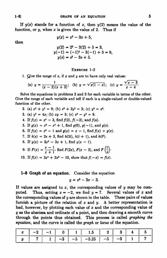
1-5 Graph of an equation. Consider the equation
y _ x2 - 3X ~ 3.
If values are assigned to x, the corresponding values of y may be com-
puted. Thus, setting x = -2, we find y = 7. Several values of x and
the corresponding values of y are shown in the table. These pairs of values
furnish a picture of the relation of x and y. A better representation is
had, however, by plotting each value of x and the corresponding value of
y as the abscissa and ordinate of a point, and then drawing a smooth curve
through the points thus obtained. This process is called graphing the
equation, and the curve is called the graph or locus of the equation.
FUNCTIONS AND GRAPHS
Y
[CHAP. 1
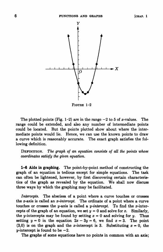
FIGURE 1-2
The plotted points (Fig. 1-2) are in the range -2 to 5 of z-values. The
range could be extended, and also any number of intermediate points
could be located. But the points plotted show about where the inter-
mediate points would lie. Hence, we can use the known points to draw
a curve which is reasonably accurate. The exact graph satisfies the fol-
lowing definition.
DEFINITION. The graph of an equation consists of all the points whose
coordinates satisfy the given equation.
1-6 Aids in graphing. The point-by-point method of constructing the
graph of an equation is tedious except for simple equations. The task
can often be lightened, however, by first discovering certain characteris-
tics of the graph as revealed by the equation. We shall now discuss
three ways by which the graphing may be facilitated.
Intercepts. The abscissa of a point where a curve touches or crosses
the x-axis is called an x-intercept. The ordinate of a point where a curve
touches or crosses the i/-axis is called a y-intercept. To find the x-inter-
cepts of the graph of an equation, we set y = and solve for x. Similarly,
the ^-intercepts may be found by setting x = and solving for y. Thus
setting y = in the equation 2x 3y =6, we find x = 3. The point
(3,0) is on the graph and the z-intercept is 3. Substituting x = 0, the
2/-intercept is found to be 2.
The graphs of some equations have no points in common with an axis;
1-6] AIDS IN GRAPHING
Y
FIGURE 1-3
for other equations there may be few or many intercepts. The intercepts
are often easily determined, and are of special significance in many prob-lems.
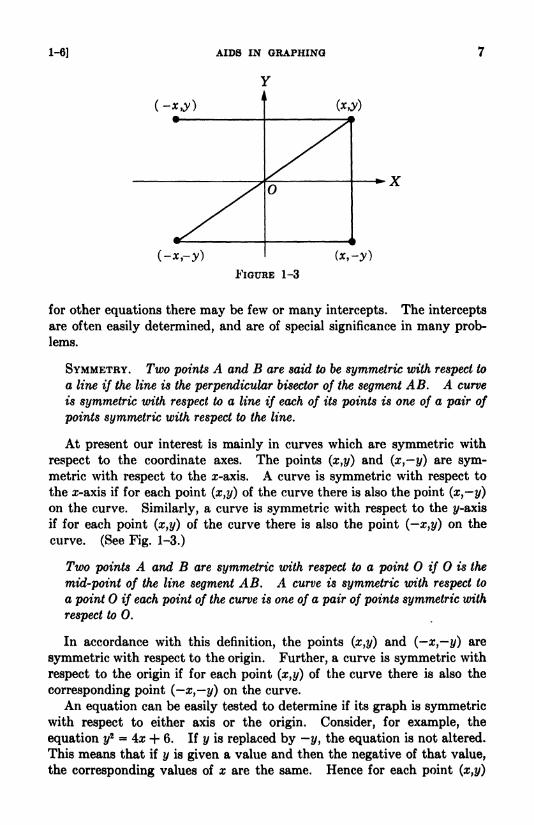
SYMMETRY. Two points A and B are said to be symmetric with respect to
a line if the line is the perpendicular bisector of the segment AB. A curve
is symmetric with respect to a line if each of its points is one of a pair of
points symmetric with respect to the line.
At present our interest is mainly in curves which are symmetric with
respect to the coordinate axes. The points (x,y) and (x, y) are sym-metric with respect to the x-axis. A curve is symmetric with respect to
the x-axis if for each point (x,y) of the curve there is also the point (x,y)on the curve. Similarly, a curve is symmetric with respect to the y-axis
if for each point (x,y) of the curve there is also the point ( x,y) on the
curve. (See Fig. 1-3.)
Two points A and B are symmetric with respect to a point if is the
mid-point of the line segment AB. A curve is symmetric with respect to
a point if each point of the curve is one of a pair of points symmetric with
respect to 0.
In accordance with this definition, the points (x,y) and ( x, y) are
symmetric with respect to the origin. Further, a curve is symmetric with
respect to the origin if for each point (x,y) of the curve there is also the
corresponding point (x,-y) on the curve.
An equation can be easily tested to determine if its graph is symmetricwith respect to either axis or the origin. Consider, for example, the
equation y2 = 4x + 6. If y is replaced by t/, the equation is not altered.
This means that if y is given a value and then the negative of that value,
the corresponding values of x are the same. Hence for each point (x,y)

8 FUNCTIONS AND GRAPHS [CHAP. 1
of the graph there is also the point (z,-i/) on the graph. The graph there-
fore is symmetric with respect to the z-axis. On the other hand, the
assigning of numerically equal values of opposite signs to x leads to dif-
ferent corresponding values for y. Hence the graph is not symmetric with
respect to the y-axis. Similarly, it may be observed that the graph is not
symmetric with respect to the origin.
From the definitions of symmetry we have the following tests.
1. If an equation is unchanged when y is replaced by y, then the graph
of the equation is symmetric with respect to the x-axis.
2. // an equation is unchanged when x is replaced by x, then the graph of
the equation is symmetric with respect to the y-axis.
3. // an equation is unchanged when x is replaced by -x and y by -y, then
the graph of the equation is symmetric with respect to the origin.
These types of symmetry are illustrated by the equations
y4 _
2y*_ x o, x2 -
4i/ + 3 -0, y = x*.
The graphs of these equations are respectively symmetric with respect to
the z-axis, the i/-axis, and the origin. Replacing x by -x and y by -y in
the third equation gives y = a:3,which may be reduced to y = x3
.
Extent of a graph. Only real values of x and y are used in graphing an
equation. Hence no value may be assigned to either which would makethe corresponding value of the other imaginary. Some equations mayhave any real value assigned to either variable. On the other hand, an
equation by its nature may place restrictions on the values of the variables.
Where there are certain excluded values, the graph of the equation is
correspondingly restricted in its extent. Frequently the admissible, and
therefore the excluded, values are readily determined by solving the equa-tion for each variable in terms of the other.
FIGURE 1-4

1-6] AIDS IN GRAPHING 9
EXAMPLE 1. Using the ideas of intercepts, symmetry, and extent, discuss the
equation 4x2 + 9t/2 =
36, and draw its graph.
Solution. Setting y = 0, we find x = 3. Hence the z-intercepts are 3
and 3. By setting x =0, the y-intercepts are seen to be 2 and 2.
The equation is not changed when x is replaced by x; neither is it changedwhen y is replaced by y. The graph therefore is symmetric with respect to both
axes and the origin.
Solving the equation for each variable in terms of the other, we obtain
y and
If 9 x2is negative, y is imaginary. Hence x cannot have a value numerically
greater than 3. In other words, x takes values from 3 to 3, which is expressed
symbolically by 3 < x < 3. Similarly, values of y numerically greater than 2
must be excluded. Hence the admissible values for y are 2 < y < 2.
A brief table of values, coupled with the preceding information, is sufficient
for constructing the graph. The part of the graph in the first quadrant (Fig. 1-4)
comes from the table;the other is drawn in accordance with the known symmetry.
EXAMPLE 2. Graph the equation x2 + 4y 12 = 0.
Solution. Setting ?/= and then x =
0, we find the ^-intercepts= 2\/3
and the ^-intercept = 3.
If x is replaced by z, the equation is unchanged. A new equation results
when y is replaced by y. Hence the graph is symmetric with respect to the
y-axis, but not with respect to the z-axis or the origin.
i i i\ i i i i Xo
FIGURE 1-5
10 FUNCTIONS AND GRAPHS [CHAP. 1
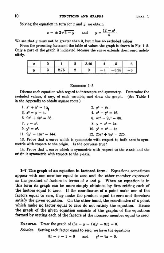
Solving the equation in turn for x and y, we obtain
and y12 -
We see that y must not be greater than 3, but x has no excluded values.
From the preceding facts and the table of values the graph is drawn in Fig. 1-5.
Only a part of the graph is indicated because the curve extends downward indefi-
nitely.
EXERCISE 1-3
Discuss each equation with regard to intercepts and symmetry,excluded values, if any, of each variable, and draw the graph,in the Appendix to obtain square roots.)
1. z2 + i/2 -
16^3. z2 = y
- 4.
5. 9z2 + 4t/2 = 36.
7. y - *3.
9. y2 = z3
.
Determine the
(See Table 1
2. i/2 = 9z.
4. z2 -*/2 = 16.
6. 4z2 -9*/
2 = 36.
8. y = x3 - 4z.
10. 1/2= x3 - 4z.
11. 9z/2 - 16z2 = 144. 12. 25z2 + 9y
2 = 225.
13. Prove that a curve which is symmetric with respect to both axes is sym-metric with respect to the origin. Is the converse true?
14. Prove that a curve which is symmetric with respect to the it-axis and the
origin is symmetric with respect to the y-axis.
1-7 The graph of an equation in factored form. Equations sometimes
appear with one member equal to zero and the other member expressedas the product of factors in terms of x and y. When an equation is in
this form its graph can be more simply obtained by first setting each of
the factors equal to zero. If the coordinates of a point make one of the
factors equal to zero, they make the product equal to zero and therefore
satisfy the given equation. On the other hand, the coordinates of a pointwhich make no factor equal to zero do not satisfy the equation. Hencethe graph of the given equation consists of the graphs of the equationsformed by setting each of the factors of the nonzero member equal to zero.
EXAMPLE. Draw the graph of (3z-
y-
l)(y*-
9z) = 0.
Solution. Setting each factor equal to zero, we have the equations
3z - y - 1 = and y2 - 9z = 0.
1-8] INTERSECTIONS OF GRAPHS 11
FIGURE 1-6
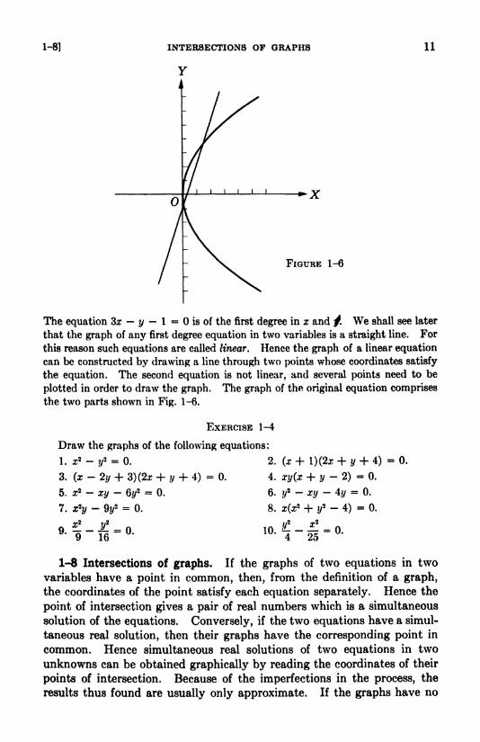
The equation 3x y 1 = is of the first degree in x and / We shall see later
that the graph of any first degree equation in two variables is a straight line. For
this reason such equations are called linear. Hence the graph of a linear equation
can be constructed by drawing a line through two points whose coordinates satisfy
the equation. The second equation is not linear, and several points need to be
plotted in order to draw the graph. The graph of the original equation comprises
the two parts shown in Fig. 1-6.
EXERCISE 1-4
Draw the graphs of the following equations:
1. x2 -if= 0.
3. (x- 2y + 3) (2* + y + 4) = 0.
5. z2 - xy - 6*/2 = 0.
7. x*y-
9t/2 - 0.
2. (x + l)(2x + y + 4)
4. xy(x + y-
2)- 0.
6. y2 - xy - 4y = 0.
8. x(x* + if-
4)= 0.
,0.^-1-0.
0.
1-8 Intersections of graphs. If the graphs of two equations in two
variables have a point in common, then, from the definition of a graph,
the coordinates of the point satisfy each equation separately. Hence the
point of intersection gives a pair of real numbers which is a simultaneous
solution of the equations. Conversely, if the two equations have a simul-
taneous real solution, then their graphs have the corresponding point in
common. Hence simultaneous real solutions of two equations in two
unknowns can be obtained graphically by reading the coordinates of their
points of intersection. Because of the imperfections in the process, the
results thus found are usually only approximate. If the graphs have no

12 FUNCTIONS AND GRAPHS [CHAP. 1
point of intersection, there is no real solution. In simple cases the solu-
tions, both real and imaginary, can be found exactly by algebraic processes.
EXAMPLE 1. Draw the graphs of the equations
y2 - 9x =
0,
3x - y- 1 = 0,
and estimate the coordinates of the points of intersection. Solve the system alge-
braically and compare results.
Solution. These are the equations whose graphs are shown in Fig. 1-6. Refer-
ring to this figure, we estimate the coordinates of the intersection points to be
(.l,-.8) and (1.6, 3.8).
To obtain the solutions algebraically, we solve the linear equation for x and
substitute in the other equation. Thus
whence
.
-3y
- 3 * 0, and3=fc \/2f
By substituting these values in the linear equation, the corresponding values for
x are found to be (5 rfc V2l)/6. Hence the exact coordinates of the intersection
points are _ _3 _I +
V21) 6 2
These coordinates to two decimal places are (1.60,3.79) and (.07, .79).
EXAMPLE 2. Find the points of intersection of the graphs of
y = x3, y = 2 - x.
\
\
FIGURE 1-7

1-9] ASYMPTOTES 13
Solution. The graphs (Fig. 1-7) intersect in one point whose coordinates
are (1,1).
Eliminating y between the equations yields
a* + x - 2 = 0, or (x-
l)(z2 + x + 2) = 0,
whence
The corresponding values of y are obtained from the linear equation. The solu-
tions, real and imaginary, are
^7 5- V^7\ -\ - V^7 5
2 2 2 2
The graphical method gives only the real solution.
EXERCISE 1-5
Graph each pair of equations and estimate the coordinates of any points of
intersection. Check by obtaining the solutions algebraically.
1. x + 2y =7, 2. 2x - y = 3,
3x - 2y = 5. 5* + 3y = 8.
3. X2 + y2=
13> 4< X2 _ 4^ = 0,
3z - 2//= 0. j/
2 = 6x.
5. x2 + 2z/2 =
9, 6. x2 + i/2 =
16,
2x - y = 0. y2 = 6x.
7. ?/= x3
,8. z/
= x2,
y = 4x. x + y- 1 = 0.
9. x2 -y2 =
9, 10. ?/= x3
4x,
r2 + j/
2 = 16. ?/= x + 4.
11. z/2 =
8j, 12. x2 + 4?/2 = 25,
2.r'- y = 4. 4x2 -lip = 8.
1-9 Asymptotes. If the distance of a point from a straight line ap-
proaches zero as the point moves indefinitely far from the origin along a
curve, then the line is called an asymptote of the curve. (See Figs. 1-8,
1-9.) In drawing the graph of an equation it is well to determine the
asymptotes, if any. The asymptotes, usually easily found, furnish an
additional aid in graphing. At this stage we shall deal with curves whose
asymptotes are either horizontal or vertical. The following examples
illustrate the procedure.
EXAMPLE 1. Determine the asymptotes and draw the graph of the equation
xy = 1.
Solution. The graph is symmetric with respect to the origin. We next notice
that if either variable is set equal to zero, there is no corresponding value of the

14 FUNCTIONS AND GRAPHS [CHAP. 1
other variable which satisfies the equation. This means that there is no intercept
on either axis, and also that zero is an excluded value for both variables. There
are no other excluded values, however.
Solving for y, the equation takes the form
Suppose we give to x successively the values 1, J, J, i, iV and so on. The cor-
responding values of y are 1, 2, 4, 8, 16, and so on. We see that as x is assigned
values nearer and nearer zero, y becomes larger and larger. In fact, by taking x
small enough, the corresponding value of y can be made to exceed any chosen
number. This relation is described by saying that as x approaches zero, y increases
without limit. Hence the curve extends upward indefinitely as the distances from
points on the curve to the 2/-axis approach zero. The y-axis is therefore an asymp-tote of the curve.
Similarly, if we assign values to x which get large without limit, then y, being
the reciprocal of x, approaches zero. Hence the curve extends indefinitely to the
right, getting nearer and nearer to the z-axis, yet never touching it. The x-axis
is an asymptote of the curve. Since there is symmetry with respect to the origin,
the graph consists of the two parts drawn in Fig. 1-8.
FIGURE 1-8
1-9] ASYMPTOTES 15
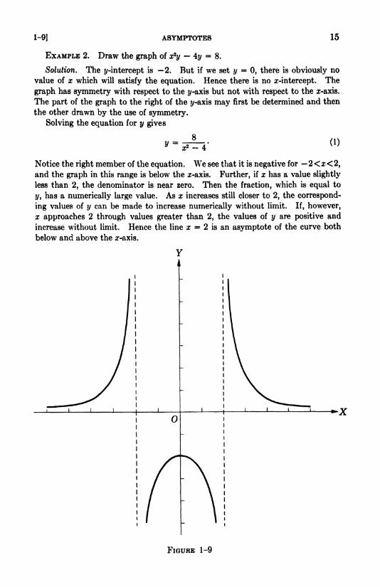
EXAMPLE 2. Draw the graph of x*y 4y = 8.
Solution. The i/-intercept is 2. But if we set y =0, there is obviously no
value of x which will satisfy the equation. Hence there is no z-intercept. The
graph has symmetry with respect to the y-axis but not with respect to the x-axis.
The part of the graph to the right of the y-axis may first be determined and then
the other drawn by the use of symmetry.
Solving the equation for y gives
y8
(1)
Notice the right member of the equation. We see that it is negative for 2 <x <2,and the graph in this range is below the z-axis. Further, if x has a value slightly
less than 2, the denominator is near zero. Then the fraction, which is equal to
y, has a numerically large value. As x increases still closer to 2, the correspond-
ing values of y can be made to increase numerically without limit. If, however,
x approaches 2 through values greater than 2, the values of y are positive and
increase without limit. Hence the line x = 2 is an asymptote of the curve both
below and above the or-axis.
_J I I L
FIGURE 1-9
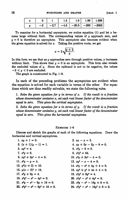
16 FUNCTIONS AND GRAPHS [CHAP. 1
To examine for a horizontal asymptote, we notice equation (1) and let x be-
come large without limit. The corresponding values of y approach zero, and
y = is therefore an asymptote. This asymptote also becomes evident when
the given equation is solved for x. Taking the positive roots, we get
X =
In this form we see that as y approaches zero through positive values, x increases
without limit. This shows that y = is an asymptote. This form also reveals
the excluded values of y. Since the radicand is not to be negative, the values
2 < y < are excluded.
The graph is constructed in Fig. 1-9.
In each of the preceding problems the asymptotes are evident whenthe equation is solved for each variable in terms of the other. For equa-
tions which are thus readily solvable, we state the following rules.
1. Solve the given equation for y in terms of x. If the result is a fraction
whose denominator contains x, set each real linear factor of the denominator
equal to zero. This gives the vertical asymptotes.
2. Solve the given equation for x in terms of y. If the result is a fraction
whose denominator contains y, set each real linear factor of the denominator
equal to zero. This gives the horizontal asymptotes.
EXERCISE 1-6
Discuss and sketch the graphs of each of the following equations. Draw the
horizontal and vertical asymptotes.
1. xy + 1 - 0.
3. (x + 1)(2/-
1)- 1.
5. xy* - 4.
7. x*y - 8.
9. sj/2 + 3t/
2 - 4 = 0.
11. 2t/ y *= 4.
13. y*(x + 8) - 10.
15. 2/(s-
2)2 = 16.
17. x*y + 9y = 4.
19 x*u* ~*~ x* " 4?v2 *~'
21. x2y - x2 - 9y + 16 - 0.
23. xY - x* - 9i/2 + 16 - 0.
2. xy - x = 3.
4. xy + 3x - 2y - 8 =
6. x*y- 9 - 0.
8. x*y* 64.
10. x2?/ + 3x2 - 4 = 0.
12. xy*- x - 4 = 0.
0.
14. x*y- x
16. xy* +18. xY +20. xY -
22. x*y-
0.
0.
+ y + 4
+ 4x + 4
y2 - 4.
* + 4y* - 0.
-16y + 9 - 0.
24. - x* - 16y2 + 9 = 0.

CHAPTER 2
FUNDAMENTAL CONCEPTS AND FORMULAS
2-1 Directed lines and segments. A line on which one direction is
defined as positive and the opposite direction as negative is called a
directed line. In analytic geometry important use is made of directed
lines. Either direction along a given line may be chosen as positive. Thex-axis and lines parallel to it are positive to the right. Vertical lines have
their positive direction chosen upward. A line not parallel to a coordinate
axis, when regarded as directed, may have either direction taken as
positive.
The part of a line between two of its points is called a segment. In
plane geometry the lengths of line segments are considered, but directions
are not assigned to the segments. In analytic geometry, however, line
segments are often considered as having directions as well as lengths.
Thus in Fig. 2-1, AB means the segment from A to B, and BA stands for
the segment from B to A. The segment AB is positive, since the direc-
tion from A to B agrees with the assigned positive direction of the line as
indicated by the arrowhead. The segment BA, on the other hand, is
negative. If there are 3 units of length between A and B, for example,then AB +3 and BA = 3. Hence, in referring to directed segments,
AB B -BA.
If A, B, and C are three points of a directed line, then the directed
segments determined by these points satisfy the equations
AB + BC = AC, AC + CB = AB, BA + AC = BC.
If B is between A and C, the segments AB, BC, and AC have the same
direction, and AC is obviously equal to the sum of the other two. Thesecond and third equations can be found readily from the first. To ob-
tain the second, we transpose BC and use the fact that BC = CB. Thus
B
A B
FIGURE 2-1 FIGURE 2-2
17

18 FUNDAMENTAL CONCEPTS AND FORMULAS
Y
[CHAP. 2
o
FIGURE 2-3
2-2 The distance between two points. In many problems the distance
between two points of the coordinate plane is required. The distance
between any two points, or the length of the line segment connecting
them, can be determined from the coordinates of the points. We shall
classify a line segment as horizontal, vertical, or slant,and derive appropriate
formulas for the lengths of these kinds of segments. In making the deriva-
tions we shall use the idea of directed segments.Let P\(xi,y) and P2(z2 ,2/) be two points on a horizontal line, and let A
be the point where the line cuts the y-axis (Fig. 2-3). We have
APZ- AP1
Similarly, for the vertical segment QiQ2 ,
QiQ2- QiB- BQ, - BQl
=2/2-
2/i.
Hence the directed distance from a first point to a second point on a hori-
zontal line is equal to the abscissa of the second point minus the abscissa
of the first point. The distance is positive or negative according as the
second point is to the right or left of the first point. A similar statementcan be made relative to a vertical segment.
Inasmuch as the lengths of segments, without regard to direction, are
often desired, we state a rule which gives results as positive quantities.
RULE. The length of a horizontal segment joining two points is the abscissa
of the point on the right minus the abscissa of the point on the left.
The length of a vertical segment joining two points is the ordinate of the
upper point minus the ordinate of the lower point.
2-2] THE DISTANCE BETWEEN TWO POINTS
Y
19
C( -2,4) 0(6,4)
Afl,0) B(5,0)
H(3,-2)
G(3,-5)
FIGURE 2-4
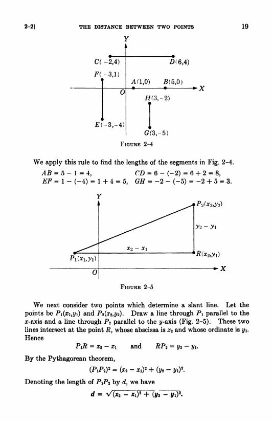
We apply this rule to find the lengths of the segments in Fig. 2-4.
,45 = 5-1=4, CD = 6 - (-2) = 6 + 2 = 8,
EF - 1 - (-4) = 1+4 =5, GH = -2 -
(-5) = -2 + 5 = 3.
o
FIGURE 2-5
We next consider two points which determine a slant line. Let the
points be PI (1,2/1) and P2Or2 ,*/2). Draw a line through P\ parallel to the
x-axis and a line through P2 parallel to the y-axis (Fig. 2-5). These two
lines intersect at the point R, whose abscissa is x2 and whose ordinate is y\.
Hence
PiR = x2-
x\ and JBP2=
t/2-
y\.
By the Pythagorean theorem,
Denoting the length of PiP by d, we have
d =

20 FUNDAMENTAL CONCEPTS AND FORMULAS [CHAP. 2
The positive square root is chosen because we shall usually be interested
only in the magnitude of the segment. We state this distance formula in
words.
THEOREM. To find the distance between two points, add the square of the
difference of the abscissas to the square of the difference of the ordinates and
take the positive square root of the sum.
In employing the distance formula either point may be designated by
(1,3/1) and the other by (0:2,2/2). This results from the fact that the two
differences involved are squared. The square of the difference of two
numbers is unchanged when the order of the subtraction is reversed.
C(-2,5)
.5(5,1)
FIGURE 2-6
EXAMPLE. Find the lengths of the sides of the triangle with the vertices
A(-2,-3), 5(5,1), and C(-2,5).
Solution. The abscissas of A and C are the same, and therefore side AC is
vertical. The other sides are slant segments. The length of the vertical side is
the difference of the ordinates. The distance formula yields the lengths of the
other sides. Thus we get
AC = 5 - (-3) = 5 + 3 =8,
AB - V(5 + 2)2 + (1 + 3)
2 - V65,
EC - V(5 + 2)2 + (1
-5)
2 = V65.
The lengths show that the triangle is isosceles.
EXERCISE 2-1
1. Plot the points A(l,0), (3,0), and C(7,0). Then find the following directed
segments: AB, AC, EC, BA, CA, and CB.
2. Given the points A (2, -3), 5(2,1), and C(2,5), find the directed distances
AB, BA, AC, CA, BC, and CB.

2-3] INCLINATION AND SLOPE OF A LINE 21
3. Plot the points 4(-l,0), B(2,0), and C(5,0), and verify the following
equations by numerical substitutions: AB + BC = AC] AC + CB = 4B;BA + AC = BC.
Find the distance between the pairs of points in problems 4 through 9:
4. (1,3), (4,7). 5. (-3,4),(2,-8).
6. (-2,-3), ri,0). 7. (5, -12), (0,0).
8. (0,-4), (3,0). 9. (2,7), (-1,4).
In each problem 10-13 draw the triangle with the given vertices and find the
lengths of the sides:
10. 4(1, -1), B(4,-l), C(4,3). 11. 4(-l,l), B(2,3), C(0,4).
12. 4(0,0), B(2,-3), C(-2,5). 13. 4(0,-3), B(3,0), C(0,-4).
Draw the triangles in problems 14-17 and show that each is isosceles:
14. 4(-2,l), B(2,-4), C(6,l). 15. 4(-l,3), B(3,0), C(6,4).
16. 4(8,3), B(l,-l), C(l,7). 17. 4(-4,4), B(-3,-3), C(3,3).
Show that the triangles 18-21 are right triangles:
18. 4(1,3), B(10,5), C(2,l). 19. 4(-3,l), B(4,-2), C(2,3).
20. 4(0,3), B(-3,-4), C(2,-2). 21. 4(4,-3), B(3,4), C(0,0).
22. Show that 4(- v/3,1), B(2\/3, -2), and C(2\/3,4) are vertices of an equi-
lateral triangle.
23. Given the points 4(1,1), B(5,4), C(2,8), and D(-2,5), show that the quad-rilateral ABCD has all its sides equal.
Determine if the points in each problem 24-27 lie on a straight line:
24. (3,0), (0,-2), (9,4). 25. (2,1), (-1,2), (5,0).
26. (-4,0), (0,2), (9,7). 27. (-!,-!), (6,-4), (-11,8).
28. If the point (x,3) is equidistant from (3, -2) and (7,4), find x.
29. Find the point on the */-axis which is equidistant from ( 5, 2) and (3,2).
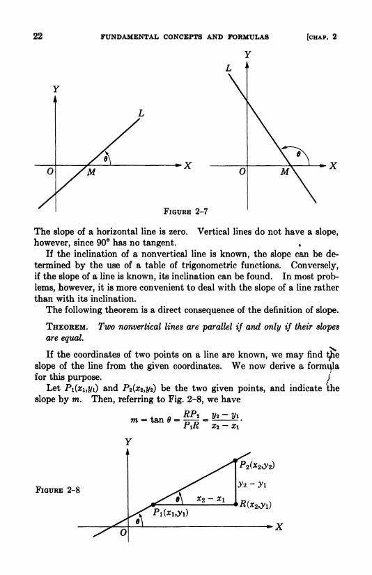
2-3 Inclination and slope of a line. If a line intersects the x-axis, the
inclination of the line is defined as the angle whose initial side extends to
the right along the x-axis and whose terminal side is upward along the line.*
In Fig. 2-7 the angle is the inclination of the line, MX is the initial side,
and ML is the terminal side. The inclination of a line parallel to the
x-axis is 0. The inclination of a slant line is a positive angle less than 180.
The slope of a line is defined as the tangent of its angle of inclination.
A line which leans to the right has a positive slope because the inclination
is an acute angle. The slopes of lines which lean to the left are negative.
* When an angle is measured from the first side to the second side, the first
side is called the initial side and the second side is called the terminal side. Fur-
ther, the angle is positive or negative according as it is measured in a counter-
clockwise or a clockwise direction.
22 FUNDAMENTAL CONCEPTS AND FORMULAS
Y
(CHAP. 2
YI
M
FIGURE 2-7
The slope of a horizontal line is zero. Vertical lines do not have a slope,
however, since 90 has no tangent. %
If the inclination of a nonvertical line is known, the slope can be de-
termined by the use of a table of trigonometric functions. Conversely,if the slope of a line is known, its inclination can be found. In most prob-
lems, however, it is more convenient to deal with the slope of a line rather
than with its inclination.
The following theorem is a direct consequence of the definition of slope.
THEOREM.are equal.
Two nonvertical lines are parallel if and only if their slopes
If the coordinates of two points on a line are known, we may findtjhe
slope of the line from the given coordinates. We now derive a formulafor this purpose. J
Let Pi(#i,2/i) and ^2(^2,2/2) be the two given points, and indicate the
slope by m. Then, referring to Fig. 2-8, we have
m = tan & =PiR
FIGURE 2-8
2-3] INCLINATION AND SLOPE OP A LINE
Y
23
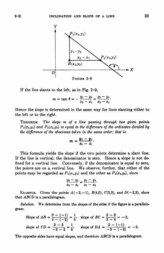
FIGURE 2-9
x
If the line slants to the left, as in Fig. 2-9,
m = tanfl= _^LJ/? = ^lU.Xz -"
X\ 2 X\
Hence the slope is determined in the same way for lines slanting either to
the left or to the right.
THEOREM. The slope m of a line passing through two given points
P\(xi,yi) and PZ(XZ,UZ) is equal to the difference of the ordinates divided by
the difference of the abscissas taken in the same order; that is
mtThis formula yields the slope if the two points determine a slant line.
If the line is vertical, the denominator is zero. Hence a slope is not de-
fined for a vertical line. Conversely, if the denominator is equal to zero,
the points are on a vertical line. We observe, further, that either of the
points may be regarded as Pi(x\,y\) and the other as Pi(xi }y^ ysince
3/2- -
1/2
EXAMPLE. Given the points A(-2,-l), (4,0), C(3,3), and Z>(-3,2), show
that ABCD is a parallelogram.
Solution. We determine from the slopes of the sides if the figure is a parallelo-
gram.
Slope of AB
slope of CD
-,
, slope of DA - __ = -3.
The opposite sides have equal slopes, and therefore ABCD is a parallelogram.
24 FUNDAMENTAL CONCEPTS AND FORMULAS [CHAP. 2
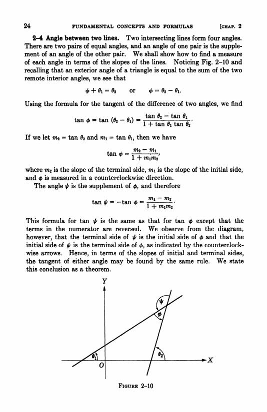
2-4 Angle between two lines. Two intersecting lines form four angles.
There are two pairs of equal angles, and an angle of one pair is the supple-
ment of an angle of the other pair. We shall show how to find a measure
of each angle in terms of the slopes of the lines. Noticing Fig. 2-10 and
recalling that an exterior angle of a triangle is equal to the sum of the two
remote interior angles, we see that
<t> + 0i - 02 or <t>= 62
-0i.
Using the formula for the tangent of the difference of two angles, we find
tan 2- tan 0i
tan <t>
- tan (02-
0i)1 + tan 0i tan 2
If we let mi - tan 2 and m\ = tan 0i, then we have
tan <(>-
where m2 is the slope of the terminal side, m\ is the slope of the initial side,
and <t> is measured in a counterclockwise direction.
The angle \l/is the supplement of
<t>,and therefore
7?l2tan ^ = -tan <t>
This formula for tan ^ is the same as that for tan < except that the
terms in the numerator are reversed. We observe from the diagram,
however, that the terminal side of ^ is the initial side of<t> and that the
initial side of ^ is the terminal side of</>,
as indicated by the counterclock-
wise arrows. Hence, in terms of the slopes of initial and terminal sides,
the tangent of either angle may be found by the same rule. We state
this conclusion as a theorem.
FIGURE 2-10

2-4] ANGLE BETWEEN TWO LINES 25
THEOREM. // <t> is an angle, measured counterclockwise, between two
lines, then
where w2 is the slope of the terminal side and m\ is the slope of the initial
side.
This formula will not apply if either of the lines is vertical, since a slope
is not defined for a vertical line. For this case, the problem would be that
of finding the angle, or function of the angle, which a line of known slope
makes with the vertical. Hence no new formula is necessary.
For any two slant lines which are not perpendicular formula (1) will
yield a definite number as the value of tan <t>. Conversely, if the formula
yields a definite number, the lines are not perpendicular. Hence we con-
clude that the lines are perpendicular when, and only when, the denomi-
nator of the formula is equal to zero. The relation 1 + m\m* = may be
written in the form
7^2 = >
mi
which expresses one slope as the negative reciprocal of the other slope.
THEOREM. Two slant lines are perpendicular if, and only if, the slope
of one is the negative reciprocal of the slope of the other.
EXAMPLE. Find the tangents of the angles of the triangle whose vertices are
4 (-2,3), #(8, -5), and C(5,4). Find each angle to the nearest degree. (See
Table II of the Appendix.)
Solution. The slopes of the sides are indicated in Fig. 2-11. Substituting in
formula (1), we get
A( -2,3) C(5,4)
5(8, -5)
FIGURE 2-11
26 FUNDAMENTAL CONCEPTS AND FORMULAS [CHAP. 2
B=33-
C - 100'.
EXERCISE 2-2
1. Give the slopes for the inclinations (a) 45; (b) 0; (c) 60; (d) 120; (e) 135.
Find the slope of the line passing through the two points in each problem 2-7 :
2. (2,3), (3,7). 3. (6, -13), (0,5).
4. (-4,8), (7,-3). 5. (5,4), (-3,-2).
6. (0,-9), (20,3). 7. (4,12), (-8,-!).
8. Show that each of the following sets of four points are vertices of a parallelo-
gram ABCD:
(a) A(2,l), B(6,l), C(4,4), D(0,4).
(b) A(-3,2), B(5,0), C(4,-3), D(-4,-l).(c) A(0,-3), fl(4,-7), (7(12, -2), D(8,2).
(d) A(-2,0), B(4,2), (7(7,7), 0(1,5).
9. Verify that each triangle with the given points as vertices is a right triangle
by showing that the slope of one of the sides is the negative reciprocal of the slope
of another side :
(a) (5,-4), (5,4), (1,0). (b) (-1,1), (3,-7), (3,3).
(c) (8,1), (l,-2), (6,-4). (d) (-1.-5), (8,-7), (3,9).
(e) (0,0), (3,-2), (2,3). (f) (0,0), (17,0), (1,4).
10. In each of the following sets, show that the four points are vertices of a
rectangle :
(a) (-6,3), (-2,-2), (3,2), (-1,7). (b) (1,2), (6,-3), (9,0), (4,5).
(c) (0,0), (2,6), (-1,7), (-3,1). (d) (5,-2), (7,5), (0,7), (-2,0).
(e) (3,2), (2,9), (-5,8), (-4,1). (f) (5,6), (1,0), (4, -2), (8,4).
11. Using slopes, determine which of the following sets of three points lie on a
straight line:
(a) (3,0), (0,-2), (9,4). (b) (2,1), (-1,2), (5,0).
(c) (-4,0), (0,2), (9,7). (d) (-1.-1), (6,-4), (-11,8).
Find the tangents of the angles of the triangle ABC in each problem 12-15.
Find the angles to the nearest degrees.
12. A(-3,-l),B(3,3),C(-l,l).13. A(-l,l),S(2,3),C(7,-7).
14. A(-3,l), 5(4,2), C(2,3).
15. A(0,3),B(-3,-4),C(2,-2).
16. The line through the points (4,3) and (-6,0) intersects the line through(0,0) and (1,5). Find the intersection angles.

2-5] THE MID-POINT OP A LINE SEGMENT 27
17. Two lines passing through (2,3) make an angle of 45. If the slope of one
of the lines is 2, find the slope of the other. Two solutions.
18. What angle does a line of slope make with a vertical line?
2-5 The mid-point of a line segment. Problems in geometry makemuch use of the mid-points of line segments. We shall derive formulas
which give the coordinates of the point midway between two points of
given coordinates.
Let PI(ZI,?/I) and P^(x^y^ be the extremities of a line segment, and let
P(x,z/) be the mid-point of PiP2. From similar triangles (Fig. 2-12), wehave
PiP PJf MP
Hence
PlN X2-
Z]
Solving for x and y gives
and
-4-
MP = y-yiNP2 2/2
-y\
_ y^ +y2"2
THEOREM. The abscissa of the mid-point of a line segment is half the sum
of the abscissas of the end points; the ordinate is half the sum of the ordinates.
This theorem may be generalized by letting P(x,y) be any division
point of the segment PiP2. Thus if
PiP = r.
then
x -
2*2- and
N(x2 ,yi)
o
FIGURE 2-12
28 FUNDAMENTAL CONCEPTS AND FORMULAS [CHAP. 2
These equations give
x = Xi + r(x2-
Xi) and y = yi + r(y2 - tfi).
If P is between PI and P2 ,as in Fig. 2-12, the segments PLP and PiP2
have the same direction, and the value of their ratio r is positive and less
than 1. If P is on PiP2 extended through P2 ,then r is greater than 1.
If P is on the segment extended through Pi, the value of r is negative.
The converse of each of these statements is true.
EXAMPLE. Find the mid-point and the trisection point nearer P2 of the segmentdetermined by Pi(-3,6) and P2(5,l).
Solution.
+ x2 _ -3 + 5 _ -_X
2 22For the trisection point we use r = .
x = xi + r(x2-
xi)= -3 + (5 + 3)
= } f
y = yi + r(y2 -2/0=6 + f(l-
6) = f .
2-6 Analytic proofs of geometric theorems. By the use of a coordinate
system many of the theorems of elementary geometry can be proved with
surprising simplicity and directness. We illustrate the procedure in the
following example.
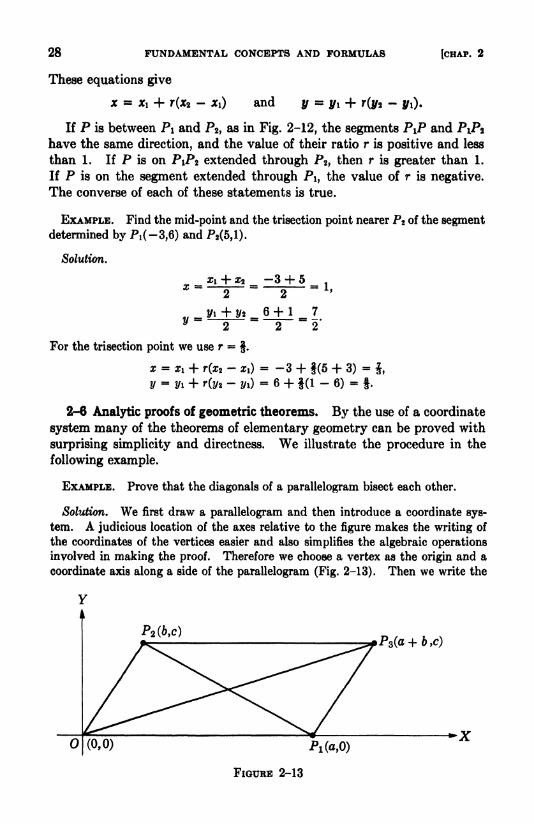
EXAMPLE. Prove that the diagonals of a parallelogram bisect each other.
Solution. We first draw a parallelogram and then introduce a coordinate sys-
tem. A judicious location of the axes relative to the figure makes the writing of
the coordinates of the vertices easier and also simplifies the algebraic operations
involved in making the proof. Therefore we choose a vertex as the origin and a
coordinate axis along a side of the parallelogram (Fig. 2-13). Then we write the
(0,0) pl(flfO)
FIGURE 2-13

2-6] ANALYTIC PROOFS OP GEOMETRIC THEOREMS 29
coordinates of the vertices as 0(0,0), Pi(a,0), P2(6,c), and P3(a + 6,c). It is
essential that the coordinates of P2 and P3 express the fact that P2P3 is equal and
parallel to OPi. This is achieved by making the ordinates of P2 and Pa the same
and making the abscissa of P3 exceed the abscissa of P2 by a.
To show that OP3 and PiP2 bisect each other, we find the coordinates of the
mid-point of each diagonal.
Mid-point of OP3 : x = ^ y = =
Mid-point of PiP,: x =
Since the mid-point of each diagonal is (a
~ '
|)'tne theorem is proved.
Note. In making a proof by this method it is essential that a general figure be
used. For example, neither a rectangle nor a rhombus (a parallelogram with all
sides equal) should be used for a parallelogram. A proof of a theorem based on a
special case would not constitute a general proof.
EXERCISE 2-3
1. Find the mid-point of AB in each of the following:
(a) X(-2,5), 5(4,-7); (b) X(7,-3), #(-3,9);
(c) A(-7 f 12), 5(11,0); (d) A(0,-7), 5(3,10).
2. The vertices of a triangle are 4(7,1), 5(-l,6), and C(3,0). Find the
coordinates of the mid-points of the sides.
3. The points A(-l,-4), 5(7,2), C(5,6), and D(-5,8) are vertices of the
quadrilateral ABCD. Find the coordinates of the mid-point of each line segment
connecting the mid-points of opposite sides.
Find the trisection points of the segment AB:
4. A(-9,-6), 5(9,6). 5. A(-5,6), 5(7,0).
6. A(-4,3), 5(8,-3). 7. A(-l,0), 5(4,6).
8. The points 4(2,2), 5(6,0), and (7(10,8) are vertices of a triangle. Deter-
mine if the medians are concurrent by finding the point on each median which
js J of the way from the vertex to the other extremity. (A median of a triangle
is a line segment joining a vertex and the mid-point of the opposite side.)
9. The points 4(2,1), 5(6, -3), and C(4,5) are vertices of a triangle. Find
the trisection point on each median which is nearer the opposite side.
10. The line segment joining A (-3,2) and 5(5, -3) is extended through each
end by a length equal to its original length. Find the coordinates of the new
ends.
11. The line segment joining A( 4, 1) and 5(3,6) is doubled in length by
having half its length added at each end. Find the coordinates of the new ends.
The points PI, P2 ,and P are on a straight line in each problem 12-15. Find
r, the ratio of PiP to PiP2 .
30 FUNDAMENTAL CONCEPTS AND FORMULAS [CHAP. 2
12. Pi(-l,-3), P2(5,l), P(2,-l). 13. PA1), P2(6,3), P(9,5).
14. PAlXPA-l), P(-l,3). 15. P l(-4 l2) fP1(l l -2) f P(ll f -10).
Give analytic proofs of the following theorems:
16. The diagonals of the rectangle are equal. [Suggestion: Choose the axes so
that the vertices of the rectangle are (0,0), (a,0), (0,6), and (a,6).]
17. The mid-point of the hypotenuse of a right triangle is equidistant from the
three vertices.
18. The line segment joining the mid-points of two sides of a triangle is parallel
to the third side and equal to half of it.
19. The diagonals of an isosceles trapezoid are equal. [Hint: Notice that the
axes may be placed so that the coordinates of the vertices are (0,0), (a,0), (6,c),
and (a 6,c).]
20. The segment joining the mid-points of the nonparallel sides of a trapezoid
is parallel to and equal to half the sum of the parallel sides.
21. The segments which join the mid-points of the sides of any quadrilateral,
if taken in order, form a parallelogram.
22. The line segments which join the mid-points of the opposite sides of a
quadrilateral bisect each other.
23. The diagonals of a rhombus are perpendicular and bisect each other.
24. The sum of the squares of the sides of a parallelogram is equal to the sum
of the squares of the diagonals.
25. The lines drawn from a vertex of a parallelogram to the mid-points of the
opposite sides trisect a diagonal.
26. The medians of a triangle meet in a point which lies two-thirds of the wayfrom each vertex to the mid-point of the opposite side.
CHAPTER 3
THE STRAIGHT LINE
3-1 Introduction. The straight line is the simplest geometric curve.
Despite its simplicity, the line is a vital concept of mathematics and enters
into our daily experiences in numerous interesting and useful ways. In
Section 1 -7 we stated that the graph of a first degree equation in x and y
is a straight line; we shall now establish that statement. Furthermore,we shall write linear equations in different forms such that each reveals
useful information concerning the location of the line which it represents.
3-2 The locus of a first degree equation. The equation
Ax + By + C = 0, (1)
where A, /?, and C are constants with A and B not both zero, is a general
equation of the first degree. We shall prove that the locus, or graph, of
this equation is a straight line by showing that all points of the locus lie
on a line and that the coordinates of all points of the line satisfy the equa-tion.
Let PI(XI,T/I) and P2 (^2,2/2) be any two points of the graph; that is,
Axl + Byi + C -0, (a)
Ax2 + By* + C - 0. (b)
By subtraction, these equations yield
and if B 7* 0,
y\-
y* = _ Ax\- xi B
The last equation shows that the slope of a line passing through two points
of the graph is -(A/B). Therefore if Ps(xi,2/i) is any other point of the
locus, the slope of the segment PiP3 is also -(A/B). From the equality
of these slopes we conclude that Pi, P2 ,and P3 ,
and hence all points of the
locus, lie on a line. To determine if the graph consists of all points of this
line, we need to show that the coordinates of any other point of the line
satisfy the given equation (1). Denoting a point of the line by P4(x4> 2/4),
we have
2/4 -y\ _ _ Az4-
x\ B31
32 THE STRAIGHT LINE [CHAP. 3
By clearing of fractions and transposing terms, this equation takes the
form
Ax* + By* - Axi - Byi - 0.
From equation (a), -Axi By\ - C, and hence
Ax* + By* + C = 0.
The point (4,1/4) satisfies the given equation. This completes the proof
except for the case in which 5 = 0. For this value of B equation (1)
reduces to
Cf _ .__ _ ,X ~ A
The coordinates of all points, and only those points, having the abscissa
(C/A) satisfy this equation. Hence the locus is a line parallel to the
2/-axis and located (C/A) units from the axis.
THEOREM. The locus of the equation Ax + By + C =0, where A, B,
and C are constants with A and B not both zero, is a straight line. If
B =0, the line is vertical; otherwise the slope is (A/B).
3-3 Special forms of the first degree equation. We shall now convert
equation (1) to other forms and interpret the coefficients geometrically.
Solving for y gives, where B 7* 0,
A C
The coefficient of x, as we have seen, is the slope of the line. By setting
x 0, we notice that the constant term is the ^-intercept. Substituting
m for the slope and b for the ^-intercept, we obtain the simpler form
y SB mx + b. (2)
This is called the slope-intercept form of the equation of a line. An equa-tion in this form makes evident the slope and the y-intercept of the line
which it represents. Conversely, the equation of a line of given slope and
2/-intercept may be written at once by substituting the proper values for
m and 6.
Illustration. The equation of the line of slope -2 and passing through
(0,5) is y = -2x + 5.
We next express equation (1) in a form which gives prominence to the
x-intercept and the y-intercept. We have
Ax + By - -C,
^ +^-1 or*
.y Cl
-C + -C"
lj or-C/A
+-C/B
X *

3-3] SPECIAL FORMS OP THE FIRST DEGREE EQUATION 33
The denominator of x in the last equation is the z-intercept and the
denominator of y is the ^-intercept. If we let a and b stand for the inter-
cepts, we have the equation
i + f-I. (3,
This is called the intercept form of the equation of a straight line. It maybe used when the intercepts are different from zero.
Equation (2) represents a line passing through (0,6). The equation
may be altered slightly to focus attention on any other point of the line.
If the line passes through (21,1/1), we have
y\= mxi + 6, and 6 = y\ mx\.
Substituting for b gives
y = mx + yi-
mx\,
and hence
y -yi = m(x -
x,). (4)
Equation (4) is called the point-slope form of the equation of a line.
If the line of equation (4) passes through the point (#2,1/2), then
and we have
y -yi =
^-E"7J(*
-*>) ^
It can readily be seen that the graph of this equation passes through the
points (xiii/i) and (0*2,1/2). This form is called the two-point form of the
equation of a straight line.
The equations (2)-(5) do not apply when the line is vertical. In this
case m is not defined, and neither could we substitute properly for the
intercepts in the forms (2) and (3). The equation of a vertical line can
be written immediately, however, if any point of the line is known. Thus
a vertical line through (xi,yi) has the abscissa x\ for all points of the line.
Hence the equation is
X = X\.
A horizontal line through (x\,yi) has m =0, and equation (4) applies.
Of course, the ordinates are all the same on a horizontal line, and we could
write the equation directly as
y ==yi*
34 THE STRAIGHT LINE [CHAP. 3
Illustrations. If a line cuts the coordinate axes so that the x-intercept
is 3 and the ^-intercept is -5, its equation by formula (3) is
1+^=1, or 5* -3s/ = 15.
The equation of the line through (1,4) with slope 3 is, by the point-
slope form,
y - 4 = 3(x + 1), .or 3x - y + 7 = 0.
To obtain the equation of the line through (3,5) and (4,1), we substi-
tute in formula (5), and have
Whence, simplifying,
1y_ 35 = - 4X - 12, or 4x + 7y = 23.
The illustrations show that formulas (2)-(5) can be employed to write,
quickly and simply, equations of lines which pass through two given points
or through one known point with a given slope. The inverse problem,that of drawing the graph of a linear equation in x and y, is likewise simple.
Since the locus is a straight line, two points are sufficient for constructingthe graph. For this purpose the intercepts on the axes are usually the
most convenient. For example, we find the intercepts of the equation3x - 4i/
= 12 to be a = 4 and b = -3. Hence the graph is the line drawn
through (4,0) and (0,-3), The intercepts are not sufficient for drawing a
line which passes through the origin. For this case the intercepts a and b
are both zero. Hence a point other than the origin is necessary.We have seen that the slope of the line corresponding to the equation
Ax + By + C = Q is -(A/B). That is, the slope is obtained from the
equation by dividing the coefficient of x by the coefficient of y and revers-
ing the sign of the result. Hence we can readily determine if the lines
represented by two equations are parallel, perpendicular, or if they inter-
sect obliquely. Lines are parallel if their slopes are equal, and we recall
that two lines are perpendicular if the slope of one is the negative of the
reciprocal of the slope of the other.
EXAMPLE 1. Find the equation of the line which passes through (-1,3) andis parallel to 4x + 3y = 2.
Solution. We shall show two ways for finding the required equation. First,
from the given equation, the slope is seen to be ($). Substituting this slopevalue and the coordinates of the given point in the point-slope formula, we have
V - 3 - -|(a + 1),
or
4x + 3y = 5.
3-3] SPECIAL FORMS OP THE FIRST DEGREE EQUATION 35
Alternatively, we notice that 4x + 3y = D is parallel to the given line for anyreal value of D. To determine D so that the line shall pass through ( 1,3), wesubstitute these coordinates for x and y and obtain
4(-l) + 3(3) =/>, or D = 5.
By using 5 for D, we have again the equation 4x + 3z/= 5.
EXAMPLE 2. A point moves so that it is equally distant from the two points
A (3,2) and (5,6). Find the equation of its locus.
Solution. From plane geometry we know that the locus is the line perpendicular
to the segment AB and passing through its mid-point. The slope of AB is 2, and
the coordinates of the mid-point are (4,4). The required slope is . Hence wewrite x + 2y = D. This equation has the proper slope, and we need to determine
D so that the line shall pass through (4,4). Substituting, we get
x + 2y = 4 + 2(4) = 12.
The required equation, therefore, is x + 2y = 12. We could also obtain this
equation by using the point-slope form (4).
EXERCISE 3-1
By solving for //, write each equation 1-12 in the slope-intercept form. In each
case give the value of the slope m and the value of the y-intercept b. Draw the
lines.
1. 3x + y = 6. 2. 3x - y- 3 = 0. 3. 4x - 2y = 3.
4. 6z + 3y = 5. 5. x + 2y + 4 = 0. 6. x - by = 10.
7. 4x - 3//= 0. 8. 2x + 7y = 0. 9. 5x + 3y = 7.
10. x - 8//= 4. 11. 7x - lly = 9. 12. x + y = 6.
By inspection, give the slope and intercepts of each line represented by equa-
tions 13-24.
13. 4x - y = 12. 14. x - y = 7. 15. x + y + 4 = 0.
16. 4x + 9y - 36. 17. 3* - 4y = 12. 18. 6* - 3y - 10 = 0.
19. x + 7y = 11. 20. 2x + 3y = 14. 21. 7x + 3z/ + 6 = 0.
22. 3x - 8/y= 5. 23. Sx + 3/y
= 4. 24. 3* + 3y = 1.
In each problem 25-36, write the equation of the line determined by the slope
m and the ^-intercept 6.
25. m = 3; b = -4. 26. m =2; 6 = 3.
27. m = -4; b = 5. 28. m = -1;6 = 1.
29. m =;6 - -2. 30. m = $ ;
6 = -6.
31. m = 0; 6 = -6. 32. m -5; 6 = 0.
33. m = -J; 6 = -8. 34. m = 0; b = -2.
35. m = 0; b = 0. 36. m = -;6 = 0.
36 THE STRAIGHT LINE [CHAP. 3
Write the equation of the line which has the ^-intercept a and the ^-intercept 6
in each problem 37-48.
37. a = 3, b - 2. 38. a = 5, 6 - 1.
39. o = 4, 6 = -3. 40. a = 7, b = -5.
41. a - -2, b = -2. 42. a = -1, 6 - -1.
43. a =,6 = i 44. o $; 6 = 1.
45. a = -y- b = f 46. a -,6 = -2.
47. a - -, 6 = -y. 48. a = f, 6 = f .
In each equation 49-60, write the equation of the line which passes throughthe point A with the slope m. Draw the lines.
49. 4(3,1); m = 2, 50. 4(-3,-5); ro = 1.
51. 4(-2,0); m =. 52. 4(0, -3); m - -4.
53. 4(-3,-6); m = -f 54. 4(5, -2); m = -f.
55. 4(0,3); m = 0. 56. 4(3,0); m = 0.
57. A(0,0); m = -f 58. 4(0,0); m = f59. 4(-5,-7); m = -6. 60. 4(9,1); m - -f
Find the equation of the line determined by the points 4 and B in each prob-lem 61-72. Check the answers by substitutions.
61. 4(3,-l); B(-4,5). 62. 4(1,5); B(4,l).
63. 4(0,2); B(4,-6). 64. 4(-2,-4); B(3,3).
65. 4(3,-2);B(3,7). 66. 4(0,0); J3(3,- 4).
67. 4(5,-); B(i-2). 68. 4(*,5); B(-2,5).
69. 4(0,1) ;B(0,0). 70. 4(3,0); (4,0).
71. 4(-l,-l); (-2,-3). 72. 4(^,1); B(-l,f).
73. Show that Ax + By = DI and Bx Ay = Z)2 are equations of perpen-dicular lines.
74. Show that the graphs of the equations
Ax + By = D!,
Ax + By = D2
are (a) the same if D\ = D2 ; (b) parallel lines if Z) A ^ D2 .
In each problem 75-84 find the equations of two lines through 4, one parallel
and the other perpendicular to the line corresponding to the given equation.Draw the lines.
75. 4(4,1); 2x - Zy + 5 = 0. 76. 4(-l,2); 2x - y = 0.
77. 4(3,4) ;Ix + 5y + 4 - 0. 78. 4(0,0) ;
x - y = 3.
79. 4(2,-3); Sx - y = 0. 80. 4(0,6); 2x - 2y 1.
81. 4(-l,l); y = 1. 82. 4(3,5); x - 0.
83. 4(7,0) ;9z + y
- 3 = 0. 84. 4(-4,0) ;4z + 3y = 3.

3-4] THE DISTANCE PROM A LINE TO A POINT 37
85. The vertices of a triangle are A(l,0), 5(9,2), and C(3,6). Find the follow-
ing:
(a) the equations of the sides;
(b) the equations of the medians and the coordinates of their common point;
(c) the equations of the altitudes and the coordinates of their common point;
(d) the equations of the perpendicular bisectors of the sides and the coordinates
of their common point.
86. The vertices of a triangle are A (-2,3), 5(6, -6), and (7(8,0). Find the
equations of the lines and the coordinates of the points pertaining to this triangle
which are called for in problem 85.
3-4 The distance from a line to a point. The distance from a line to a
point can be found from the equation of the line and the coordinates of the
point. We shall derive a formula for this purpose. We observe first that
the distance from a vertical line to a point is immediately obtainable by
taking the difference of the abscissa of the point and the z-intercept of the
line. Hence no additional formula is needed for this case.
Let the equation of a slant line be written in the form
Ax + By + C =Q, (1)
and let Pi(x\,yi) be any point not on the line. Since the line is a slant
line, B ^ 0. Consider now the line through PI parallel to the given line,
and the line through the origin perpendicular to the given line, whose
equations respectively are
Ax + By + C 1 -0, (2)
Bx - Ay = 0. (3)
The required distance d (Fig. 3-1) is equal to the segment PQ, where Pand Q are the intersection points of the perpendicular line and the parallel
lines. The simultaneous solutions of equations (1) and (3), and equations
(2) and (3) give the intersection points
-BC \ -AC' -BC'
We employ the formula for the distance between two points to find the
length of PQ. Thus
I
(C~
C/)2*2
-t-
(^ 2 + fi2)2
_ (C - C'?(A* + B2) (C - C')
2
(A* + B*)2 A2 + B2
'
and
C-C'

38 THE STRAIGHT LINU [CHAP. 3
FIGURE 3-1
Since the line of equation (2) passes through PI(ZI,I/I), we have
Axi + Byi + C' = 0, and C' = -Axi -Byi.
Hence, substituting for C",
Ax^ 4- #wi 4- Cd =
To remove the ambiguity as to sign, we agree to give the radical in the
denominator the sign of B. In other words, the sign of the denominator
is selected so that the coefficient of y\ is positive. A consequence of this
choice of signs may be found by referring to the figure again, where P Pi
is parallel to the i/-axis and P (.ri,2/o) is a point of the given line. Since Pis a point on the line, we have
Now if we replace t/ by yi in the left side of this equation, we get an ex-
pression which is not equal to zero. The expression is positive if y\ > y$
and negative if y\ < y<>. That is, the expression for d is positive if PI is
above the line and negative if PI is below the line. We may therefore
regard the distance from a line to a point as a directed distance.
The preceding discussion establishes the following theorem :
THEOREM. The directed distance from the slant line Ax + By + C =
to the point Pi (#1,2/1) is given by the formula
* ^ + *" + C(4)
where the denominator is given the sign of B. The distance is positive if
the point PI is above the line, and negative if P\ is below the line.

3-4] THE DISTANCE FROM A LINE TO A POINT 39
Y
-4,1)
^3(9,0)
FIGURE 3-2
If equation (1) is divided by VA* + B2,the form
Ax + By + C _VA*+B*
is obtained. This is called the normal form of the equation of a line.
When an equation is in the normal form, the distance from the line to a
point is given by substituting the coordinates of the point in the left mem-ber of the equation. By substituting the coordinates of the origin, the
constant term is seen to be the perpendicular, or normal, distance to the
origin.
EXAMPLE 1. Find the distance from the line I2y
points Pi(3,-5), P2(-4,l), and P3(9,0).
5x - 26 to each of the
Solution. We write the equation in the form 5x + I2y + 26 = 0. The
required distances are then found by making substitutions in formula (4). Hence
, -5(3) + 12(-5) + 26 49
-5(-4) + 12(1) + 26 _ 58
13 13'
, -5(9) + 12(0) + 26d3==
13
19
13'
The positive sign is used in the denominators because the coefficient of y is posi-
tive. The signs of the results show that PI and PS are below the line and that Pz
is above the line (Fig. 3-2).
EXAMPLE 2. Find the distance between the parallel lines 15x Sy 51 =0and 15z - Sy + 68 = 0.
Solution. The distance can be found by computing the distance from each line
to a particular point. To minimize the computations, we find the distance from
each line to the origin. Thus
A 15(0)-
8(0)- 51 _ -51 _. __ _ ^
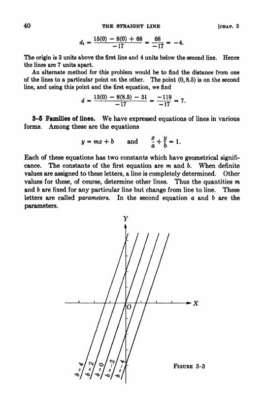
40 THE STRAIGHT LINE [CHAP. 3
, _ 15(0)-
8(0) + 68 68 _ Ad2TIT :=T7
~ ~ 4 *
The origin is 3 units above the first line and 4 units below the second line. Hence
the lines are 7 units apart.
An alternate method for this problem would be to find the distance from one
of the lines to a particular point on the other. The point (0, 8.5) is on the second
line, and using this point and the first equation, we find
, _ 15(0)-
8(8.5)- 51 -119 _ .
3-5 Families of lines. We have expressed equations of lines in various
forms. Among these are the equations
y = mx + 6 and M- 1 -
Each of these equations has two constants which have geometrical signifi-
cance. The constants of the first equation are m and b. When definite
values are assigned to these letters, a line is completely determined. Other
values for these, of course, determine other lines. Thus the quantities mand 6 are fixed for any particular line but change from line to line. These
letters are called parameters. In the second equation a and 6 are the
parameters.
FIGURE 3-3
3-6] FAMILY OF LINES THROUGH INTERSECTION OF TWO LINES 41
A linear equation with only one parameter is obtained if the other
parameter is replaced by a fixed value. The resulting equation repre-
sents all lines with a particular property if the remaining parameter is
allowed to vary. Each value assumed by the parameter yields an equa-tion which represents a definite line. The collection of lines defined by a
linear equation with one parameter is called a family, or system, of lines.
For example, if m =3, the point-slope equation becomes
y = 3z + b.
This equation represents the family of lines of slope 3, one line for each
value of b. There are, of course, infinitely many lines in the family. In
fact, a line of the family passes through each point of the coordinate plane.
Figure 3-3 shows a few lines of the family corresponding to the indicated
values of the parameter b.
EXAMPLE 1 . Write the equation of the system of lines defined by each of the
following conditions:
(a) parallel to 3x - 2y =5,
(b) passing through (5, 2),
(c) having the product of the intercepts equal to 4.
Solutions. The following equations are easily verified to be those required.
(a) 3x - 2y = D. (b) y + 2 = m(x - 5).
(c)-a+ j^= 1, or 4* + oty-4n.
EXAMPLE 2. Write the equation of the system of lines which are parallel to
5x + 12/y + 7 = 0. Find the members of the family which are 3 units distant
from the point (2,1).
Solution. Each member of the family 5x -f 12// 4- C = is parallel to the
given line. We wish to find values of C which will yield lines 3 units from the
point (2,1), one passing above and the other below the point. Using the formula
for the distance from a line to a point, we obtain the equations
5(2) + 12(1) + C _ 5(2) + 12(1) + C _13
3'
13~*
The roots are C = 17 and C = 61. Hence the required equations are
5* + \2y + 17 = and 5z + I2y- 61 - 0.
3-6 Family of lines through the intersection of two lines. The equation
of the family of lines passing through the intersection of two given lines
can be written readily. To illustrate, we consider the two intersecting
lines
From the left members of these equations we form the equation
(2*-
30 + 5) + fc(4x + y-
11) - 0, (1)

42 THE STRAIGHT LINE [CHAP. 3
where fc is a parameter. This equation is of the first degree in x and y
for any value of k. Hence it represents a system of lines. Furthermore,each line of the family goes through the intersection of the given lines.
We verify this statement by actual substitution. The given lines intersect
at (2,3). Then, using these values for x and t/, we get
(4-9 + 5) + fc(8 + 3- 11) =0,+ fc(0)
-0,
= 0.
This result demonstrates that equation (1) is satisfied by the coordinates
(2,3) regardless of the value of k. Hence the equation defines a family of
lines passing through the intersection of the given lines.
More generally, let the equations
C2=
define two intersecting lines. Then the equation
(A& + Biy + Ci) + k(A& + B*y + C2)=
represents a system of lines through the intersection of the given lines.
To verify this statement, we first observe that the equation is linear for
any value of A. Next we notice that the coordinates of the intersection
point reduce each of the parts in parentheses to zero, and hence satisfy the
equation for any value of k.
EXAMPLE. Write the equation of the system of lines through the intersection
of x - 7y + 3 = and 4z + 2y - 5 - 0. Find the member of the family which
has the slope 3.
Solution. The equation of the system of lines passing through the intersection
of the given lines is
(x- 7y + 3) + k(4x + 2y - 5) =
0,
or, collecting terms,
(1 + 4fc)z + (-7 + 2k)y + 3 - 5* = 0.
The slope of each member of this system, except for the vertical line, is ^Equating this fraction to the required slope gives
=
3, and k = 2.
The member of the system for k * 2 is 9x 3y 7 = 0.
EXERCISE 3-2
Find the distance from the line to the point in each problem 1-6.
1. 5x + I2y + 60 = 0; (3,2). 2. 4x - 3y = 15; (4,1).
3-6) FAMILY OF LINES THROUGH INTERSECTION OF TWO LINES 43
3. x + y- 3 - 0; (4,5). 4. 3* + y - 10; (-3,-!).
5. -2x + 5y + 7 = 0; (6,0). 6. y =7; (3, -8).
Determine the distance between the pair of parallel lines in each problem 7-10.
7. 4x - 3y - 9 =0, 4z - 3z/
- 24 0.
8. 12z + 5y =13, 12x + 5i/
= 104.
9. 15z - 8#- 34 =
0, 15x - 8y + 51 = 0.
10. x + y + 7 -0, z + y- 11 - 0.
Write the equation of the system of lines possessing the given property in each
problem 11-18. In each case assign three values to the parameter and draw the
corresponding lines.
11. Parallel to 7x - 4y = 3.
12. Passing through (-3,4).
13. Having the x-intercept twice the y-mtercept.
14. Perpendicular to 2z 5y + 3 = 0.
15. Having the y-intercept equal to 4.
16. Having the sum of the intercepts equal to 10.
17. Through the intersection of x - 2y + 7 = and 5x - ly - 3 = 0.
18. Forming with the coordinate axes a triangle of area 16.
Tell what geometric property is possessed by all the lines of each system in
problems 19-26.
19. y = mx + 4. 20. y = 2x + b.
21. 9x + 2y = k. 22. y + 4 - m(x - 3).
25. (4x - 7y - 7) + ky = 0. 26. (4* + y + 1) + fc(3x + ly) = 0.
27. In the preceding problems 19-26 determine the line of the system which
passes through (3,0).
28. Write the equation of the family of lines of slope 3, and find the two
members passing 5 units from the origin.
In each problem 29-34 find the equation of the line which passes through the
intersection of the pair of lines and satisfies the other given condition.
29. 3x + y- 2 -
0, x + by- 4 =
0; through (5,2).
30. 5z -f 3y + 2 = 0, x - y- 2 - 0; m = -3.
31. x - lit/=
0, 3s + y- 5 = 0; a vertical line.
32. 6s - 2y = 3, x - 5y = 4; m = 0.
33. 3x - 4y - 2 0, 3x + 4y + 1 =0; intercepts are equal.
34. 2ar-i/-5 =0, x + i/-4 = 0; passing through (0,0).
35. The sides of a triangle are on the lines defined by 2x 3y + 4 =0,
x + y + 3 =0, and 5x - 4y - 20 0. Without solving for the vertices, find
the equations of the altitudes.
44 THE STRAIGHT LINE [CHAP. 3
36. Find the equations of the bisectors of the angles formed by the lines
4x + 3#- 12 - and 5x - I2y
- 60 = 0. [Suggestion: Let P(x,y) be a point
on a bisector and use the fact that each point of a bisector is equally distant from
the sides.]
37. Find the equations of the bisectors of the angles formed by the lines
x + 2y + 3 * and 2x + y- 2 = 0.
38. Write the equation Ax + By + C = in normal form. Show that in
this form the coefficient of x is equal to cos w and the coefficient of y is equal to
sin w, where w is the inclination of the perpendicular segment drawn from the
origin to the line.
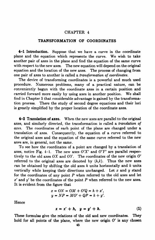
CHAPTER 4
TRANSFORMATION OF COORDINATES
4-1 Introduction. Suppose that we have a curve in the coordinate
plane and the equation which represents the curve. We wish to take
another pair of axes in the plane and find the equation of the same curve
with respect to the new axes. The new equation will depend on the original
equation and the location of the new axes. The process of changing from
one pair of axes to another is called a transformation of coordinates.
The device of transforming coordinates is a powerful and much used
procedure. Numerous problems, many of a practical nature, can be
conveniently begun with the coordinate axes in a certain position and
carried forward more easily by using axes in another position. We shall
find in Chapter 5 that considerable advantage is gained by the transforma-
tion process. There the study of second degree equations and their loci
is greatly simplified by the proper location of the coordinate axes.
4-2 Translation of axes. When the new axes are parallel to the original
axes, and similarly directed, the transformation is called a translation of
axes. The coordinates of each point of the plane are changed under a
translation of axes. Consequently, the equation of a curve referred to
the original axes and the equation of the same curve referred to the newaxes are, in general, not the same.
To see how the coordinates of a point are changed by a translation of
axes, notice Fig. 4-1. The new axes O'X' and O'Y' are parallel respec-
tively to the old axes OX and OF. The coordinates of the new origin 0'
referred to the original axes are denoted by (h,k). Thus the new axes
can be obtained by shifting the old axes h units horizontally and fc units
vertically while keeping their directions unchanged. Let x and y stand
for the coordinates of any point P when referred to the old axes and let
x 1 and y' be the coordinates of the point P when referred to the new axes.
It is evident from the figure that
x . ON - OM + O'Q - h + x',
y = NP = MO' + QP = k + y'.
Hence
* = *' + /,, y = y' + fc. (1)
These formulas give the relations of the old and new coordinates. Theyhold for all points of the plane, where the new origin 0' is any chosen
45

46 TRANSFORMATION OF COORDINATES
y
[CHAP. 4
X'
point of the plane. Holding for all points of the plane, the formulas
apply in particular to the points of a curve. Consequently, the substitu-
tions x f + h for x, and yf + k for y in the equation of a curve referred to
the original axes yield the equation of the same curve referred to the trans-
lated axes.
EXAMPLE 1. Find the transformed equation of
xy - 3x + 2y- 12 =
if the origin is translated to the point ( 2,3).
Solution. Here h = 2 and k = 3. Hence the translation equations (1) are
x = x' - 2 and y -y' + 3.
Making these substitutions in the given equation, we get
(xr -
2)Q/' + 3)-
3(x'-
2) + 2(y' + 3)- 12 -
0,
x'y' + 3z' - 2y'- 6 - 3*' + 6 + 2y' + 6 - 12 =
0,
x'y1 -6 = 0.
The transformed equation has no first degree terms. The graph is more easily
constructed by use of this equation and the new axes. The origin of the new axes
is 2 units to the left of the old origin and 3 units upward. Both sets of axes andthe graph are drawn in Fig. 4-2.
EXAMPLE 2. Translate the axes so that the equation
2z2 + 3#2 - 10* + ISy + 26 -
is transformed to a simpler form.
Solution. We do not know in advance what the translation should be. Hencewe use the translation formulas with h and k unknown. Thus we have
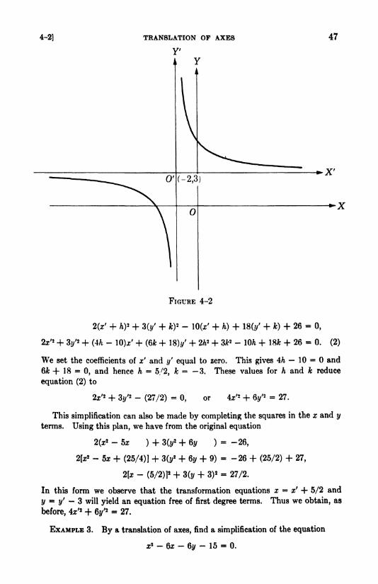
4-2] TRANSLATION OF AXES
Y'
47
0' (-2,3)
FIGURE 4-2
2(x' + h)* + 3(y' + k)*-
10(x' + fc) +W + ft) + 26 -0,
2x'2-f 3i/
2 + (4/i-
10)*' + (6* + 18)//' + 2fc2 + 3*2 - lOfc + 18* + 26 = 0. (2)
We set the coefficients of x' and y' equal to zero. This gives 4h 10 = and
6& + 18 =0, and hence h = 5/2, k = 3. These values for h and k reduce
equation (2) to
2x'2 + 3?/'2 -
(27/2) -0, or 4x'2
-h 6i//2 = 27.
This simplification can also be made by completing the squares in the x and y
terms. Using this plan, we have from the original equation
-fa ) + 3(#2 + 6y )
= -26,
2[x2 - 5x + (25/4)] + 3(y
2 + 6y + 9)= -26 + (25/2) + 27,
2[x-
(5/2)]' + 3(y + 3)'- 27/2.
In this form we observe that the transformation equations x = x' + 5/2 and
y =y' 3 will yield an equation free of first degree terms. Thus we obtain, as
before, 4z/2 + 6y'2 = 27.
EXAMPLE 3. By a translation of axes, find a simplification of the equation
x2 - 6x - 6y- 15 = 0.
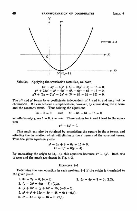
48 TRANSFORMATION OP COORDINATES
Y[CHAP. 4
FIGURE 4-3
-X'
Solution. Applying the translation formulas, we have
(x' + h)*-
6(z' + h)-
6(i/' + A;)- 15 = 0,
x'2 + 2Ax' + h2 Qxf
6/z> 6t/'' Qk 15 = 0,
x'* + (2h- 6X -
6y' + (h*- 6/1 - Qk - 15) = 0.
The a;'2 and i/' terms have coefficients independent of h and k, and may not be
eliminated. We can achieve a simplification, however, by eliminating the x' term
and the constant terms. Thus solving the equations
2^-6 = and A2 - 6h - 6A; - 15 =
simultaneously gives h =3, k = 4. These values for h and k lead to the equa-
tion
x'2 - 6i/'- 0.
This result can also be obtained by completing the square in the x terms, and
selecting the translation which will eliminate the x' term and the constant terms.
Thus the given equation yields
x2 - 6x + 9 - 60 + 15 + 9,
(x-
3)2 - 6(y + 4).
By translating the origin to (3, 4), this equation becomes x 12 =of axes and the graph are drawn in Fig. 4-3.
Both sets
EXERCISE 4-1
Determine the new equation in each problem 1-8 if the origin is translated to
the given point.
1. 3x + 2y =6; (4, -3). 2. 5x - 4y + 3 - 0; (1,2).
3. (2/-2)' = 6(*-3);(2,3).
4. (x + 3)2 + (y + 5)
2 - 25; (-3,-5).
5. x* + y* + I2x - Sy + 48 -0; (-6,4).
6. x2 - 4* - ly + 46 - 0; (2,6).

4-3] ROTATION OP AXES 49
7. xy - x - y- 10 = 0; (1,1).
8. x-8* + 3r- y + 3;(l,-2).
In each problem 9-14 give the point to which the origin must be translated in
order that the transformed equation shall have no first degree term. Find also
the new equation.
9. x2 + if- 2x - 4y - 4 = 0.
11. xy - 2x - 3// -8 = 0.
13. 2x2 + 4//2 + I2x + 8y + 4 = 0.
10. 2x2 + 2//2 - 8x + 5 = 0.
12. x2 -y*- Sx + Qy + 3 = 0.
14. 9x2 + 4y2 - 8y = 0.
In each problem 15-18 eliminate the constant term and one of the first degree
terms.
15. z/2 -
6</ + 4x + 5 = 0.
17. i/2 + lOx + 4y + 24 = 0.
16. x2 - 2x - 8i/- 15 = 0.
18. i/2 -
4t/- z + 1 = 0.
4-3 Rotation of axes. When the hew axes have the same origin but di-
rections different from the original axes, the transformation is called a
rotation of axes. That is, the new axes may be obtained by rotating the
original axes through an angle about the origin.
We shall derive transformation formulas, for a rotation through an
angle 0, which express the old coordinates in terms of the new coordinates.
In Fig. 4-4 the coordinates of the point P are (x,y) referred to the original
axes OX and OF, and are (*',?/') when referred to the new axes OX' and
OF'. We notice that x = OM and y = A/P, x' = OS and y'= SP. The
segment RS is drawn parallel to the x-axis and NS is parallel to the y-axis.
Hence we have
x
y
= O.V - MN = O.V - RS = x' cos -y' sin 0,
MP = MR + RP = NS + RP = x' sin + y' cos 0.
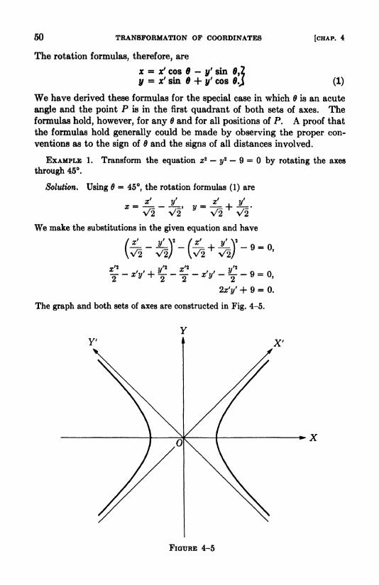
50 TRANSFORMATION OF COORDINATES [CHAP. 4
The rotation formulas, therefore, are
x = x' cos - yfsin 0,2
y = *' sin 9 + yfcos 9J (1)
We have derived these formulas for the special case in which 6 is an acute
angle and the point P is in the first quadrant of both sets of axes. Theformulas hold, however, for any and for all positions of P. A proof that
the formulas hold generally could be made by observing the proper con-
ventions as to the sign of and the signs of all distances involved.
EXAMPLE 1. Transform the equation x* y* 9 = by rotating the axes
through 45.
Solution. Using = 45, the rotation formulas (1) are
= JL. _ yL = JL_ ]LX ~~
V2 V2y ~
\/2 \/2*
We make the substitutions in the given equation and have
2x'y' + 9 = 0.
The graph and both sets of axes are constructed in Fig. 4-5.
FIGURE 4-5
4-4] SIMPLIFICATION OF SECOND DEGREE EQUATIONS 51
EXAMPLE 2. _Find the acute angle of rotation such that the transformed equa-tion of 2x2 + V3xy + y*
= 8 will have no x'y' term.
Solution. We employ the rotation formulas in order to find the required
angle 6. Substituting for x and ?/, we get
2(z' cos -y' sin 6)* + ^(x f
cos 6 - y' sin 6)(x' sin 6 + yfcos 6)
+ (x' sin 6 + y' cos BY = 8.
We perform the indicated multiplications, collect like terms, and obtain
(2 cos2 6 + V3 sin 6 cos + sin20)z'
2 + (-2 sin cos + \/3 cos2
- \/3 sin2B)x'y' + (2 sin2 6 - >/3 sin cos + cos2 0)y'
2 = 8. (2)
Since the x'y' term is to vanish, we set its coefficient equal to zero. Thus we have
-2 sin 6 cos 6 + V3(cos2 - sin26)= 0.
Using the identities sin 26 = 2 sin 6 cos and cos 28 = cos2 sin20, the equation
takes the form
-sin 20+ V3cos20 =0,
whence
tan 20 = \/3, 20 =60, = 30.
A rotation of 30 eliminates the x'y' term. This value of reduces equation (2) to
EXERCISE 4-2
Find the new equation in problems 1-8 when the axes are rotated through the
given angle.
1. V3x -y = 4;
= 60. 2. x + y = 6; = 45.
3. Xy = 4; = 45. 4. r> + if= a2
;
= 40.
5. x2 + TV + y2 = 1
;
= 45. 6. z2 - V3xy + 2*/2 = 2; = 30.
7. x2 -4xt/ + 4?/
2 - 8\/5x - 4v/5y = 0; = arc tan J.
8. z2 + V&ry + 2y2 = 3; = arc tan v/3.
Find the angle of rotation in each problem 9-12 such that the transformed
equation will have no x'y' term.
9. 3xy + y- 2 - 0. 10. x2 - xy + 5 - 0.
11. x2 - 3xy + 4y2 + 7 = 0. 12. j2 + 3xy - x + y = 0.
Simplification of second degree equations. In the two preceding
sections we used transformations which led to simpler forms of various first
and second degree equations. In the next chapter we shall study second
degree equations systematically. To facilitate this study, it will be desir-
able to have equations in their simplest forms. We now consider the sim-
plest forms of second degree equations.
52 TRANSFORMATION OP COORDINATES [CHAP. 4
The general second degree, or quadratic, equation in x and y is repre-
sented by
Ax* + Bxy + Cy* + Dx + Ey + F = 0. (1)
At least one of the constants A, B, and C must be different from zero in
order for the equation to be of the second degree. We assume, too, that
not all the coefficients of terms involving one of the variables is zero.
That is, both x and y appear in the equation.
If B =0, and A and C are both different from zero, we may complete
the squares in the x and y terms, as in Example 2, Section 4-2. Then it
is easy to find the translation which will reduce the equation to the form
AV2 + C'y'2 + F' = 0.
If B and one of the coefficients A and C is also zero, we may find the
translation, as in Example 3, Section 4-2, which will reduce the equation
(1) to one of the forms
By2 + D'x' = or AV2 + E'y' = 0.
If B ^ 0, an essential part of the simplification consists in obtaining a
transformed equation lacking the product term x'y'. We shall show howto determine immediately an angle of rotation which will serve for this
purpose. In equation (1) we substitute the right members of the rotation
formulas for x and y. This gives, after collecting like terms, the equation
AV2 + B'x'y' + C'y'* + D'x' + E'y' + F' -0,
where the new coefficients are
A' - A cos2 + B sin cos + C sin26,
B' - B cos 26- (A- C) sin 26,
C' = A sin2 6 - B sin 6 cos 6 + C cos26,
D' - D cos 6 + E sin 6,
E' = E cos 6 - D sin 6,
F' -F.
The x f
yf term will vanish only if its coefficient is zero. Hence 6 must
satisfy the equation
B' = B cos 26 - (A -C) sin 26 = 0.
If A 76 C, the solution is
Btan 26 * A-C
This formula yields the angle of rotation except when A = C. If A =C,
the coefficient of x'y' is B cos 26. Then the term vanishes by giving 6 the
value 45. Thus we see that an equation of the form (1) with an xy term
can be transformed into an equation free of the product term x'y'.

4-4] SIMPLIFICATION OF SECOND DEGREE EQUATIONS 53
We summarize the preceding results in the following theorem.
THEOREM. A second degree equation
in which B = can be transformed by a translation into one of the forms
A'x'* + C'y'* + F = 0,
A!*'* + E'y' = 0, (2)
cy2 + D'X' = o.
// B j& 0, one of these forms can be obtained by a rotation and a translation
(if necessary). The angle of rotation 6 (chosen acute) is obtained fromthe equation
tan2g = Br > if A * C,A C
= 46, if A = C.
By this theorem we see how to find the value of tan 26. The rotation
formulas, however, contain sin 6 and cos 6. These functions can be ob-
tained from the trigonometric identities
/I- cos 26 a ll
sin 6 = */^
cos 6 = A/+ cos 26
The positive sign is selected before each radical because we shall restrict 6
to an acute angle.
EXAMPLE. Reduce the equation
73jr2 - 72xy + 52//2 + lOOr - 200// + 100 =
to one of the forms (2).
Solution. We first transform the equation so that the product term x'y' will
be lacking. To find the angle of rotation, we have
.
ofl _ B__
-72 _ -24tan 20- J^Tc- 73^-52- 7
'
whence
-7cos2*-
T5
. . /A -cos20 4 , . /I + cos 26 3sin 6 HB A/ = - and cos 6 = '
Hence
2 5 \ 2 5
The rotation formulas are then
3z' 4t/' , 4x'x ^
^ anc| ^ =

54 TRANSFORMATION OP COORDINATES [CHAP. 4
FIGURE 4-6
By substituting for x and y in the given equation and simplifying, we get
z'2 + 4i/'2 - 4x' - Sy' + 4 = 0.
Completing the squares in the x' and yf
terms, this equation becomes
Cr'-2) 2 +4(2/'- 1)2 -4=0.
Finally, a translation to the point (2,1) yields the desired form
x"2 + 42/"2 -4 = 0.
It is much easier to draw the graph from this equation than by using the original
equation. The graph and the three sets of axes are constructed in Fig. 4-6.
EXERCISE 4-3
Translate the axes so that the constant term is eliminated. Draw both sets of
axes and the graph:
1. 3z - 4y = 6. 2. x = 6.
Rotate the axes through an acute angle such that the x' or the y' term is elimi-
nated:
3. 3x - 4t/= 6. 4. x + y = 0.
Reduce each of the equations 5-8 to one of the simplified forms (2).
5. x2 -2xy + y*
- 8V2t, -8 = 0.
6. 3x2 + 2V3xy + 2/2 - 2x - 2vHy - 16 = 0.
7. 73*2 - 72xy + My* + 380x - 1602/ + 400 = 0.
8. 7x2 + 4Sxy - 7y2 - 150z - 5Qy + 100 - 0.
4-4] SIMPLIFICATION OF SECOND DEGREE EQUATIONS 55
9. Show that the graph of the quadratic equation in one variable
Ax2 + Dx + F = is one line, two parallel lines, or that no real value of x satis-
fies the equation, according as the discriminant Z)2 4AF is zero, positive, or
negative.
Write the left members of the following equations as the product of two linear
factors. Draw the graphs corresponding to the real factors.
10. z2 - x - 6 = 0. 11. z2 + 6z + 9 = 0.
12. z2 + x - 1 = 0. 13. x2 + x + 1 = 0.
14. Work out all the steps of the rotation transformation which is applied to
equation (1), Section 4-4.
CHAPTER 5
THE SECOND DEGREE EQUATION
6-1 Introduction. In this chapter we shall study second degree, or
quadratic, equations in two variables. The general quadratic equation in
x and y may be expressed in the form
Ax2 + Bxy + <V + Dx + Ey + F = 0. (1)
The study of this kind of equation in some respects is less simple than the
case of the linear equation. Any linear equation in two variables has a
locus, and the locus is a straight line. In contrast, not all second degree
equations have loci, and those having loci represent different types of
curves. Our principal interest, however, will be in equations which have
loci.
The locus of a quadratic equation in two variables is called a conic
section or, more simply, a conic. This designation comes from the fact
that the locus or curve can be obtained as the intersection of a right cir-
cular cone and a plane.* Conic sections were investigated, particularly
by Greek mathematicians, long before analytic methods were introduced.
Various properties of conies were discovered and this phase of geometryreceived much emphasis. Today the interest in conic sections is enhanced
by numerous important theoretical and practical applications which have
been found.
Obviously, different kinds of conic sections are possible. A plane, not
passing through the vertex of a cone, may cut all the elements of one nappeand make a closed curve (Fig. 5-1). If the plane is parallel to an element,
the intersection extends indefinitely far along one nappe but does not cut
the other. The plane may cut both nappes and make a section of two
parts, with each extending indefinitely far along a nappe. In addition
to these sections the plane may pass through the vertex of the cone and
determine a point, a line, or two intersecting lines. An intersection of
this kind is sometimes called a degenerate conic. The section consisting
of two intersecting lines approaches two parallel lines if the cone is madeto approach a cylinder by letting the vertex recede indefinitely far. For
this reason, two parallel lines are classed with the degenerate conies.
* A right circular cone is the surface generated by a line which passes througha fixed point on a fixed line and moves so that it makes a constant angle with the
fixed line. The fixed point is the vertex and the generating line in any positionis called an element. The vertex separates the cone into two parts called nappes.
56

5-2] THE SIMPLIFIED EQUATIONS OF CONICS 57
FIGURE 5-1
5-2 The simplified equations of conies. Despite the interesting geo-
metric way in which conies first became known, we shall approach their
study as loci of second degree equations rather than as the intersections
of planes and cones. In our study we shall take advantage of the simpli-
fied equations
A* + Cy2 + F = 0, (2)
Cy2 + Dx = 0, (3)
Xx2 + Ey = 0,
'
(4)
which were obtained in Section 4-4.
Normally, equations (2)-(4) represent conies. There are exceptional
cases, however, depending on the values of the coefficients. The excep-
tional cases are not our main interest, but we do notice them. Equa-tion (2) has no locus if A, C, and F are all of the same sign, for then there
are no real values of x and y for which the terms of the left member add
to zero. If F =0, and A and C have the same sign, only the coordinates of
the origin satisfy the equation. Selections of values for the coefficients
may be variously made so that equation (2) represents two intersecting

58 THE SECOND DEGREE EQUATION [CHAP. 5
lines, two parallel lines, or one line. An equation of the form (3) or (4)
always has a locus, but the locus is a line if the coefficient of the first degree
term is zero. The point and line loci of second degree equations are called
degenerate conies, as was previously noted.
Aside from the exceptional cases, we shall discover that equations of
the form (2) represent different types of curves, depending on the relative
values of A and C. We shall consider the cases in which (a) A = C,
(b) A and C have the same sign but are unequal, and (c) A and C have
opposite signs. The equations (3) and (4) are not essentially different so
far as their loci are concerned. This statement may be justified by noting
that a rotation of 90 will transform either equation into one having the
form of the other.
6-3 The parabola. We shall consider first equations (3) and (4). Eachof these equations has only one second degree term, and in this respect
is simpler than equation (2). By division and transposition we reduce
the equations to the forms
(5)
(6)
which will be found more convenient. The locus of an equation of either
of these forms, or which -can be reduced to one of these forms, is called a
parabola. Restricting our attention for the moment to equation (5), weobserve at once certain characteristics of its locus. The graph passes
through the origin and is symmetric with respect to the x-axis. If a > 0,
x may have any positive value or zero, but may have no negative value.
As x increases, the values of y increase numerically. Hence the graph
FIGURE 5-2
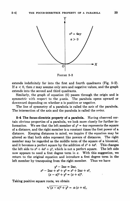
5-4] THE FOCUS-DIRECTRIX PROPERTY OF A PARABOLA
Y
59
O
FIGURE 5-3
extends indefinitely far into the first and fourth quadrants (Fig. 5-2).
If a < 0, then x may assume only zero and negative values, and the graph
extends into the second and third quadrants.
Similarly, the graph of equation (6) passes through the origin and is
symmetric with respect to the #-axis. The parabola opens upward or
downward depending on whether a is positive or negative.
The line of symmetry of a parabola is called the axis of the parabola.
The intersection of the axis and the parabola is called the vertex.
6-4 The focus-directrix property of a parabola. Having observed cer-
tain obvious properties of a parabola, we look more closely for further in-
formation. We see that the left member of y*= 4ax represents the square
of a distance, and the right member is a constant times the first power of a
distance. Keeping distances in mind, we inquire if the equation may be
altered so that both sides represent like powers of distances. The right
member may be regarded as the middle term of the square of a binomial,
and it becomes a perfect square by the addition of x2 + 4a2. This changes
the left side to x2 + 4a2 + ?/2
,which is not a perfect square. The left side
now appears to need a first degree term in x. With this suggestion, wereturn to the original equation and introduce a first degree term in the
left member by transposing from the right member. Thus \ve have
i/2 - 2ax
x2 - 2ax + a2 + y2
(x-
a)2 + ?/
Taking positive square roots, we obtain
: x2 + 2ax + a2,
(x + a)2
.
(x + a),
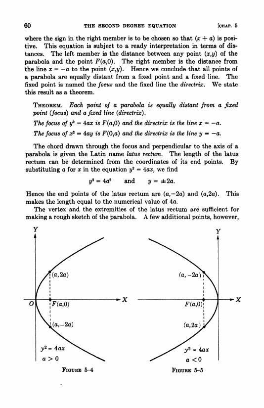
60 THE SECOND DEGREE EQUATION [CHAP. 5
where the sign in the right member is to be chosen so that (x + a) is posi-
tive. This equation is subject to a ready interpretation in terms of dis-
tances. The left member is the distance between any point (x,y) of the
parabola and the point F(a,0). The right member is the distance from
the line x - a to the point (x,y). Hence we conclude that all points of
a parabola are equally distant from a fixed point and a fixed line. Thefixed point is named the focus and the fixed line the directrix. We state
this result as a theorem.
THEOREM. Each point of a parabola is equally distant from a fixed
point (focus) and a fixed line (directrix).
The focus of y*= 4az is F(a,0) and the directrix is the line x = a.
The focus of x2 = 4ay is F(0,a) and the directrix is the line y = a.
The chord drawn through the focus and perpendicular to the axis of a
parabola is given the Latin name latus rectum. The length of the latus
rectum can be determined from the coordinates of its end points. Bysubstituting a for x in the equation y
2 = 4ox, we find
4a2 and y = 2a.
ThisHence the end points of the latus rectum are (a, 2a) and (a,2a).
makes the length equal to the numerical value of 4a.
The vertex and the extremities of the latus rectum are sufficient for
making a rough sketch of the parabola. A few additional points, however,
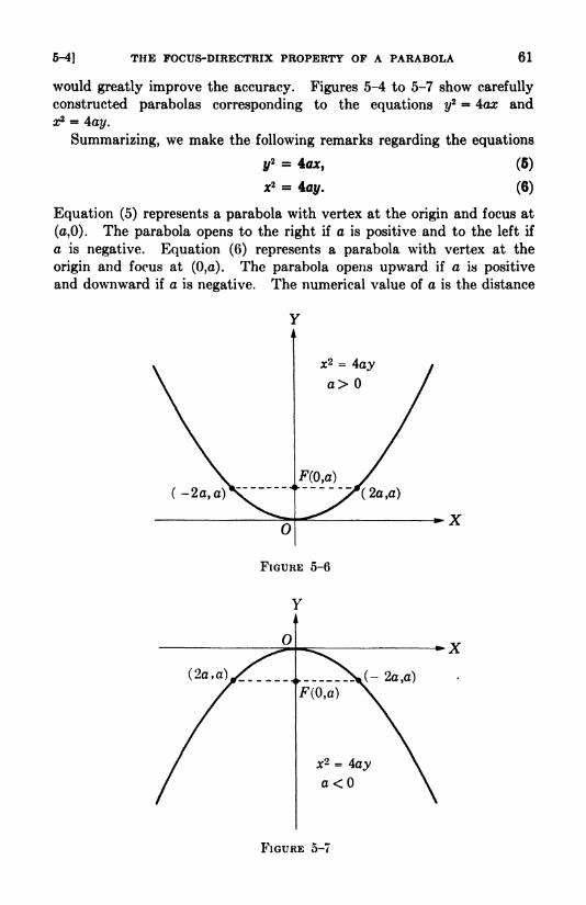
5-4] THE FOCUS-DIRECTRIX PROPERTY OF A PARABOLA 61
would greatly improve the accuracy. Figures 5-4 to 5-7 show carefully
constructed parabolas corresponding to the equations y2 = 4ax and
rr2 =
4ai/.
Summarizing, we make the following remarks regarding the equations
y2 = 4, (6)
x2 = 4ay. (6)
Equation (5) represents a parabola with vertex at the origin and focus at
(a,0). The parabola opens to the right if a is positive and to the left if
a is negative. Equation (6) represents a parabola with vertex at the
origin and focus at (0,a). The parabola opens upward if a is positive
and downward if a is negative. The numerical value of a is the distance
FIGURE 5-7
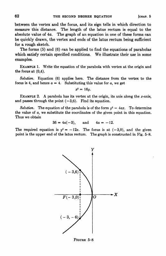
62 THE SECOND DEGREE EQUATION [CHAP. 5
between the vertex and the focus, and its sign tells in which direction to
measure this distance. The length of the latus rectum is equal to the
absolute value of 4a. The graph of an equation in one of these forms can
be quickly drawn, the vertex and ends of the latus rectum being sufficient
for a rough sketch.
The forms (5) and (6) can be applied to find the equations of parabolas
which satisfy certain specified conditions. We illustrate their use in some
examples.
EXAMPLE 1 . Write the equation of the parabola with vertex at the origin and
the focus at (0,4).
Solution. Equation (6) applies here. The distance from the vertex to the
focus is 4, and hence a = 4. Substituting this value for a, we get
x2 -16*/.
EXAMPLE 2. A parabola has its vertex at the origin, its axis along the x-axis,
and passes through the point (3,6). Find its equation.
Solution. The equation of the parabola is of the form */2 = 4ax. To determine
the value of a, we substitute the coordinates of the given point in this equation.
Thus we obtain
36 = 4o(-3), and 4a = -12.
The required equation is y2 = I2x. The focus is at (3,0), and the given
point is the upper end of the latus rectum. The graph is constructed in Fig. 5-8.
FIGURE 5-8

5-4) THE FOCUS-DIRECTRIX PROPERTY OF A PARABOLA
y
63
(-' I).
FIGURE 5-0
EXAMPLE 3. The equation of a parabola is j*2 = 6#. Find the coordinates
of the focus, the equation of the directrix, and the length of the latus rectum.
Solution. The equation is of the form (6), where a is negative. Hence the
focus is on the negative //-axis and the parabola opens downward. From the
equation 4a =6, we find a = 3/2. Therefore the coordinates of the focus
are (0, 3'2) and the directrix is y = 3 '2. The length of the latus rectum is
numerically equal to 4a, and in this case is 6. The latus rectum extends 3 units
to the left and 3 units to the right of the focus. The graph may be sketched by
drawing through the vertex and the ends of the latus rectum. For more accurate
graphing a few additional points could be plotted. (See Fig. 5-9.)
EXERCISE 5-1
Find the coordinates of the focus, the coordinates of the ends of the latus
rectum, and the equation of the directrix of each parabola in problems 1-6. Sketch
each curve.
1. //2 = 4x. 2. y
2 = -16*. 3. x* = -10#.
4. * = \2y. 5. y* + 3* = 0. 6. x2 - By = 0.
Write the equation of the parabola with vertex at the origin and which satisfies
the given conditions in each problem 7-16.
7. Focus at (3,0). 8. Focus at (-4,0).
9. Directrix is x + 6 = 0. 10. Directrix is y- 4 = 0.
11. Latus rectum 12, and opens downward.
12. Focus on the ?y-axis, and passes through (2,8).
13. Axis along the ?/-axis, and passes through (4, 3).
14. Ends of latus rectum are (3, 6) and (3,6).
15. Opens to the left, and passes through ( 1, 1).
16. Opens to the right, and the length of the latus rectum is 16.

64 THE SECOND DEGREE EQUATION [CHAP. 5
17. A cable suspended from supports which are at the same height and 400 feet
apart has a sag of 100 feet. If the cable hangs in the form of a parabola, find its
equation, taking the origin at the lowest point.
18. Find the width of the cable of problem 17 at a height 50 feet above the
lowest point.
6-5 The ellipse. We next consider the equation
Ax* + Cy* + F =0, (2)
where A and C have the same sign and F has the opposite sign. If A = C,
we may write the equation as x2 + y2 = F/A. The left member is the
square of the distance of any point (x,y) from the origin. Hence the locus
is a circle and the right member is the square of the radius. Indicating
the radius by r, we have the more suggestive form
x* + 3,2= r2. (7)
If A 9* C, the locus of equation (2), or an equation reducible to this
form, is defined as an ellipse. By setting x and y in turn equal to zero,
we find the squares of the intercepts on the axes to be F/A and F/C.
Using a2 = -F/A and 62 = -F/C, equation (2) becomes
b*(8)
The intercepts are thus brought into prominence, and for still other
reasons this form will be convenient. We shall regard a and b as positive,
and for definiteness take a > 6.
We notice first that the graph of equation (8) is symmetric with respect
to both coordinate axes. Solving for x and y in turn, we have
and
FIGURE 5-10

5-6] THE FOCI OF AN ELLIPSE 65
These equations show that y2 must not exceed 62
,and z2 must not exceed
a2. In other words, the permissible values of the variables are given by
-a < x < a and -6 < y < b. The graph (Fig. 5-10) cuts the z-axis at the
points V'(-a,0) and F(a,0), and cuts the y-axis at B'(0,-6) and B(0,6).
The segment F'7(= 2a) is called the major axis of the ellipse, and B'B(= 26)
is the minor axis. The ends of the major axis are called vertices. The
intersection of the major and minor axes is the center of the ellipse. (The
designation of the vertices by V and V comes from the first letter in
the word vertex.)
FIGURE 5-11
The graph of
(9)
is drawn in Fig. 5-11. The ellipses represented by equations (8) and (9)
are alike except for their positions relative to the coordinate axes.
6-6 The foci of an ellipse. An important property of the ellipse is the
fact that the sum of the distances from each point of the ellipse to two
fixed points is constant. The fixed points, called foci, are on the major
axis and equidistant from the center. We shall prove this property of
the ellipse.

THE SECOND DEGREE EQUATION [CHAP. 5
Figure 5-12 shows the graph of equation (8). The points F'(~c,0)
and F(c,0) denote the foci, where for the moment c is undetermined. For
the vertex V we have F'V + FV = F'V + V'F' = 2a. Thus the con-
stant 2a is the sum of the distances from the vertex to the foci. Hence
we need to show that the sum of the distances from any point on the
ellipse to the foci is equal to 2a. By considering next the special point B,
the value of c may be determined. In order that F'B + FB should be
equal to 2a, each of these segments must have a length equal to a. This
gives, from the right triangle OFfi, the relation c2 = a2 62. Using this
relation and the equation of the ellipse, we next show that F'P + FP is
equal to 2a, where P(x,y) is any point of the ellipse. Denoting this sum
by S, we have
S = V(x + c)2 + i/
2 + \/(x-
c)2 + y*.
Whence, squaring and collecting like terms,
(a)
S2 - 2z2 + 2if + 2c2 + 2Vx4 - 2cV + c4 + 2xV + 2c2//
2 + ?/4
. (b)
If we replace c2 by a2 - 62,the radicand becomes
a4 + 64 + x4 + ?/- 2a262 - 2aV + 2a2
?/2 + 26V -
2b*y* + 2x*if.
An examination of this expression reveals that it is equal to
(a2 + 62 - z2 -
?/)2
if the signs of each of the terms 2a262,2a2
?/
2,and 26V are reversed. The
equation of the ellipse, (8), yields 262x2 + 2a2#2 - 2a262 =
0, which shows
that the signs of the three terms may be reversed without changing the
value of the radicand. Hence we have
FIGURE 5-12

5-6]
and
THE FOCI OF AN ELLIPSE
2 + 2a2 - 2b2 + 2(a2 + b2 - rr
2 -?/2)= 4a2
67
We chose the positive square root of the radical of equation (b). This is
necessary because the radical is the product of the two positive radicals
of equation (a). That we chose the positive square root may be observed
from the figure. We notice that a2 + 62 > x2 + ?/2
,and hence a2 + b2
x27/2 > 0. It is necessary also to select the positive square root of
4a2,since S is the sum of two positive quantities. We state the result as
a theorem.
THEOREM. The sum of the distances from each point of an ellipse to two
fixed points (foci) of the major axis is constant and equal to the length of
the major axis.
The foci of -^ + |2= 1
c2 - a2 - b2.
the points ( r,0) and (r,0), where
The foci of-2-f ,
-2= 1 are the points (0, c) and (0,c), where
still c2 = a2 - b\
The chord through a focus and perpendicular to the major axis is called
a latus rectum. Substituting x = c in the equation of the ellipse (8) and
using the relation c2 = a2fo2
,the points (e, b2
a) and (r,62'a) are found
to be the ends of one latus rectum. Hence the length of the latus rectum
is 262/a. The ellipse and each latus rectum are drawn in Fig. 5-13.
Y
5-13

68 THE SECOND DEGREE EQUATION [CHAP. 5
6-7 The eccentricity of an ellipse. The ratio c/a is called the eccen-
tricity e of the ellipse. The shape of the ellipse depends on the value of
its eccentricity. For example, suppose that we visualize an ellipse in
which the major axis remains constant, while e starts at zero and ap-
proaches unity. If e = 0, the equations e = c/a and b2 = a2 c2 show that
c = and a = 6. The two foci are then coincident at the origin and the
ellipse is a circle. As e increases, the foci separate, each receding from
the origin, and 6 decreases. As e approaches 1, c approaches a, and 6
approaches 0. Thus the ellipse, starting as a circle, becomes narrow, with
all its points near the major axis.
EXAMPLE 1. Find the equation of the ellipse with foci at (0,4) and a vertex
(at 0,6.)
Solution. The location of the foci shows that the center of the ellipse is at the
origin, that the equation is of the form (9), antf that c = 4. The given vertex,
6 units from the center, makes a = 6. Using the relation b2 = a2 c2,we find
b2 = 20. Hence the required equation is
36+
20= L
EXAMPLE 2. Sketch the ellipse 9z2 + 25y2 = 225.
Solution. Dividing by 225 gives the form
25+
9= L
Since the denominator of x2is greater than the denominator of y
2,the major axis

5-7] THE ECCENTRICITY OF AN ELLIPSE 69
is along the z-axis. We see also that a2 = 25, b2 = 9, and c = Vo2 62 = 4.
Hence the vertices are at (5,0), the ends of the minor axis at (0,3), and the
foci at (4,0). The length of a latus rectum is 262/a = 18/5. The locations of
the ends of the axes and the ends of each latus rectum are sufficient for makinga sketch of the ellipse. Figure 5-14 shows the curve with several important
points indicated.
EXERCISE 5-2
Find the coordinates of the foci, the ends of the axes, and the ends of each
latus rectum in problems 1-10. From this information sketch the curves.
1?/ + x*
-1 2 4-^-1lm
25+ 9~~
} ' *'169
+ 25"lu
3*' + ?y
'-
1 4y*
+ J2 -1*' T69M44" IB 4>
25+
16~ l '
r2/v2 r2
?v2
R *i !/ i a *
i
"i5
-49+
25=L 8
-9-+ r *'
7. 25.r2 + 4//2 = 100. 8. x2 + 4*/
2 = 9.
9. 4.r2 + if
= 4. 10. 2J2 + 3?/2 = 12.
Write the equations of the ellipses whose axes coincide with the coordinate
axes, and which satisfy the conditions given in problems 11-18.
11. Vertex (4,0); end of minor axis (0,3).
12. Focus (2,0); vertex (5,0).
13. Focus (0, 4); minor axis 4.
14. Minor axis 12; vertex (9,0).
15. Focus (3,0); length of latus rectum 9.
16. End of minor axis (5,0); length of latus rectum f$.
17. Passing through (3,5) and (7,5/3).
18. Passing through (3,V2) and (v/6,2).
19. The perimeter of a triangle is 30, and the points (0, 5) and (0,5) are two
of the vertices. Find the locus of the third vertex.
20. A point moves so that the sum of its distances from (3,0) and (3,0) is 8.
Find the equation of its path.
21. Find the equation of the locus of the mid-points of the ordinates of the
circle a:2 + /y
2 = 36.
22. The ordinates of a curve are k times the ordinates of the circle x2 + ?/2 = a2
.
Show that the curve is an ellipse if A; is a positive number different from 1 .
23. A line segment of length 12 moves with its ends always touching the coor-
dinate axes. Find the equation of the locus of the point on the segment which
is 4 units from the end, in contact with the x-axis.
24. A rod of length a+ b moves with its ends in contact with the coordinate
axes. Show that the point at a distance a from the end in contact with the z-axis
describes an ellipse if a ^ 6.
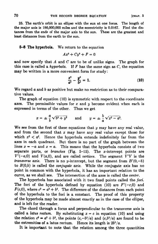
70 THE SECOND DEGREE EQUATION [CHAP. 5
25. The earth's orbit is an ellipse with the sun at one focus. The length of
the major axis is 186,000,000 miles and the eccentricity is 0.0167. Find the dis-
tances from the ends of the major axis to the sun. These are the greatest and
least distances from the earth to the sun.
6-8 The hyperbola. We return to the equation
Ax2 + Cy* + F =
and now specify that A and C are to be of unlike signs. The graph for
this case is called a hyperbola. If F has the same sign as C, the equation
may be written in a more convenient form for study :
We regard a and b as positive but make no restriction as to their compara-tive values.
The graph of equation (10) is symmetric with respect to the coordinate
axes. The permissible values for x and y become evident when each is
expressed in terms of the other. Thus we get
x =|Vb* + y
2 and y =^Vz2 - a2
.
We see from the first of these equations that y may have any real value,
and from the second that x may have any real value except those for
which x2 < a2. Hence the hyperbola extends indefinitely far from the
axes in each quadrant. But there is no part of the graph between the
lines x = a and x = a. This means that the hyperbola consists of two
separate parts, or branches (Fig. 5-15). The x-intercept points are
V'(-aff) and V(a,0), and are called vertices. The segment V'V is the
transverse axis. There is no ?/-mtercept, but the segment from B'(0,-b)to B(Q,b) is called the conjugate axis. While the conjugate axis has no
point in common with the hyperbola, it has an important relation to the
curve, as we shall see. The intersection of the axes is called the center.
The hyperbola has associated with it two fixed points called the foci.
The foci of the hyperbola defined by equation (10) are F'(-c,0) and
F(c,0), where c2 = a2 + 62. The difference of the distances from each point
of the hyperbola to the foci is a constant. The proof of this propertyof the hyperbola may be made almost exactly as in the case of the ellipse,
and is left for the reader.
The chord through a focus and perpendicular to the transverse axis is
called a latus rectum. By substituting x = c in equation (10) and usingthe relation c2 a2 + 62
,the points (c,-6
2/a) and (c,b
2/a) are found to be
the extremities of a latus rectum. Hence its length is 262/a.
It is important to note that the relation among the three quantities
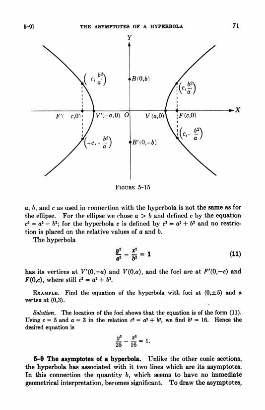
5-9] THE ASYMPTOTES OF A HYPERBOLA
Y
71
FIGURE 5-lf>
a, 6, and c as used in connection with the hyperbola is not the same as for
the ellipse. For the ellipse we chose a > b and defined c by the equation
c2 = a2 - 62;for the hyperbola c is defined by c2 = a2
4- b2 and no restric-
tion is placed on the relative values of a and b.
The hyperbola
b2 (11)
has its vertices at F'(0,-a) and F(0,a), and the foci are at F'(0,-c) and
F(0,c), where still c2 = a2 + 62.
EXAMPLE. Find the equation of the hyperbola with foci at (0,5) and a
vertex at (0,3).
Solution. The location of the foci shows that the equation is of the form (11).
Using c = 5 and a = 3 in the relation c2 = a2 + fr2
,we find 62 = 16. Hence the
desired equation is
._._ 1
25 16
6-9 The asymptotes of a hyperbola. Unlike the other conic sections,
the hyperbola has associated with it two lines which are its asymptotes.In this connection the quantity b, which seems to have no immediate
geometrical interpretation, becomes significant. To draw the asymptotes,
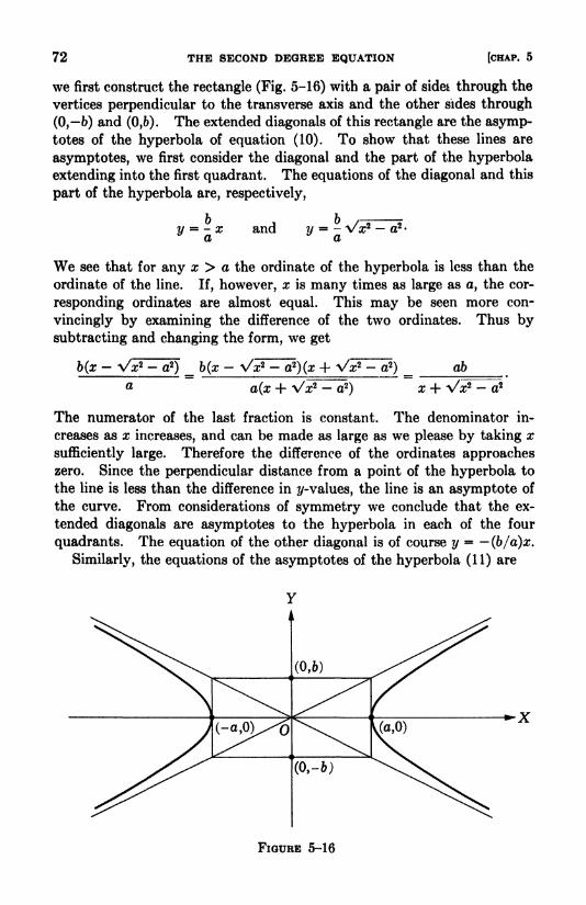
72 THE SECOND DEGREE EQUATION [CHAP. 5
we first construct the rectangle (Fig. 5-16) with a pair of sidei through the
vertices perpendicular to the transverse axis and the other sides through
(0, b) and (0,6). The extended diagonals of this rectangle are the asymp-totes of the hyperbola of equation (10). To show that these lines are
asymptotes, we first consider the diagonal and the part of the hyperbola
extending into the first quadrant. The equations of the diagonal and this
part of the hyperbola are, respectively,
y --x and
We see that for any x > a the ordinate of the hyperbola is less than the
ordinate of the line. If, however, x is many times as large as a, the cor-
responding ordinates are almost equal. This may be seen more con-
vincingly by examining the difference of the two ordinates. Thus bysubtracting and changing the form, we get
b(x- Vx* - a2
) = b(x- Vx* - a2
)(s + Vx* - a2)
a a(x + Vx2 - a2)
ab
x + Vrr2 - a2
The numerator of the last fraction is constant. The denominator in-
creases as x increases, and can be made as large as we please by taking x
sufficiently large. Therefore the difference of the ordinates approacheszero. Since the perpendicular distance from a point of the hyperbola to
the line is less than the difference in ^-values, the line is an asymptote of
the curve. From considerations of symmetry we conclude that the ex-
tended diagonals are asymptotes to the hyperbola in each of the four
quadrants. The equation of the other diagonal is of course y = -(b/d)x.
Similarly, the equations of the asymptotes of the hyperbola (11) are
FIGURE 5-16
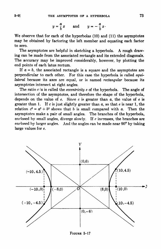
6-9] THE ASYMPTOTES OP A HYPERBOLA 73
anda
I'
We observe that for each of the hyperbolas (10) and (11) the asymptotes
may be obtained by factoring the left member and equating each factor
to zero.
The asymptotes are helpful in sketching a hyperbola. A rough draw-
ing can be made from the associated rectangle and its extended diagonals.
The accuracy may be improved considerably, however, by plotting the
end points of each latus rectum.
If a =6, the associated rectangle is a square and the asymptotes are
perpendicular to each other. For this case the hyperbola is called equi-
lateral because its axes are equal, or is named rectangular because its
asymptotes intersect at right angles.
The ratio c/a is called the eccentricity e of the hyperbola. The angle of
intersection of the asymptotes, and therefore the shape of the hyperbola,
depends on the value of e. Since c is greater than a, the value of e is
greater than 1. If c is just slightly greater than a, so that e is near 1, the
relation c2 = a2 + b2 shows that b is small compared with a. Then the
asymptotes make a pair of small angles. The branches of the hyperbola,enclosed by small angles, diverge slowly. If c increases, the branches are
enclosed by larger angles. And the angles can be made near 90 by taking
large values for e.
FIGURE 5-17
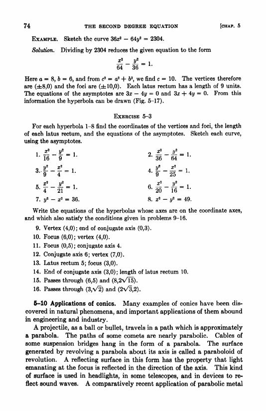
74 THE SECOND DEGREE EQUATION [CHAP. 5
EXAMPLE. Sketch the curve 36x2 -64i/
2 = 2304.
Solution. Dividing by 2304 reduces the given equation to the form
- _^! = 1
64 36
Here a = 8, b = 6, and from c2 = a2 + 62,we find c = 10. The vertices therefore
are (8,0) and the foci are (10,0). Each latus rectum has a length of 9 units.
The equations of the asymptotes are 3x 4y = and 3x + 4y = 0. From this
information the hyperbola can be drawn (Fig. 5-17).
EXERCISE 5-3
For each hyperbola 1-8 find the coordinates of the vertices and foci, the length
of each latus rectum, and the equations of the asymptotes. Sketch each curve,
using the asymptotes.
1 _?.! _ t = 1 9 - ^ = 1
16 9 36 64
3 f. - * - 1 4 V* _ xl - I6t9 4
~ L 4 '
9" 25~ IB
* 2f _ l! _ i 6* j -
i5<4 21
"20 16
" *'
7. ?/- x2 = 36. 8. z2 -
*/
2 = 49.
Write the equations of the hyperbolas whose axes are on the coordinate axes,
and which also satisfy the conditions given in problems 9-16.
9. Vertex (4,0); end of conjugate axis (0,3).
10. Focus (6,0); vertex (4,0).
11. Focus (0,5); conjugate axis 4.
12. Conjugate axis 6; vertex (7,0).
13. Latus rectum 5; focus (3,0).
14. End of conjugate axis (3,0); length of latus rectum 10.
15. Passes through (6,5) and (8,2Vl5).
16. Passes through (3,\/2) and (2^,2).
6-10 Applications of conies. Many examples of conies have been dis-
covered in natural phenomena, and important applications of them abound
in engineering and industry.
A projectile, as a ball or bullet, travels in a path which is approximatelya parabola. The paths of some comets are nearly parabolic. Cables of
some suspension bridges hang in the form of a parabola. The surface
generated by revolving a parabola about its axis is called a paraboloid of
revolution. A reflecting surface in this form has the property that light
emanating at the focus is reflected in the direction of the axis. This kind
of surface is used in headlights, in some telescopes, and in devices to re-
flect sound waves. A comparatively recent application of parabolic metal
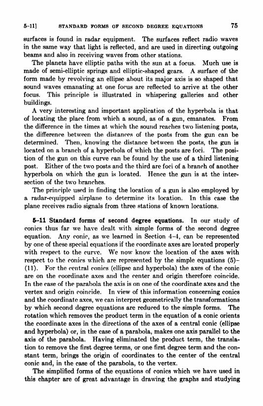
5-11) STANDARD FORMS OF SECOND DEGREE EQUATIONS 75
surfaces is found in radar equipment. The surfaces reflect radio waves
in the same way that light is reflected, and are used in directing outgoingbeams and also in receiving waves from other stations.
The planets have elliptic paths with the sun at a focus. Much use is
made of semi-elliptic springs and elliptic-shaped gears. A surface of the
form made by revolving an ellipse about its major axis is so shaped that
sound waves emanating at one focus are reflected to arrive at the other
focus. This principle is illustrated in whispering galleries and other
buildings.
A very interesting and important application of the hyperbola is that
of locating the place from which a sound, as of a gun, emanates. Fromthe difference in the times at which the sound reaches two listening posts,
the difference between the distances of the posts from the gun can be
determined. Then, knowing the distance between the posts, the gun is
located on a branch of a hyperbola of which the posts are foci. The posi-
tion of the gun on this curve can be found by the use of a third listening
post. Either of the two posts and the third are foci of a branch of another
hyperbola on which the gun is located. Hence the gun is at the inter-
section of the two branches.
The principle used in finding the location of a gun is also employed bya radar-equipped airplane to determine its location. In this case the
plane receives radio signals from three stations of known locations.
6-11 Standard forms of second degree equations. In our study of
conies thus far we have dealt with simple forms of the second degree
equation. Any conic, as we learned in Section 4-4, can be represented
by one of these special equations if the coordinate axes are located properlywith respect to the curve. We now know the location of the axes with
respect to the conies which are represented by the simple equations (5)-
(11). For the central conies (ellipse and hyperbola) the axes of the conic
are on the coordinate axes and the center and origin therefore coincide.
In the case of the parabola the axis is on one of the coordinate axes and the
vertex and origin coincide. In view of this information concerning conies
and the coordinate axes, we can interpret geometrically the transformations
by which second degree equations are reduced to the simple forms. Therotation which removes the product term in the equation of a conic orients
the coordinate axes in the directions of the axes of a central conic (ellipse
and hyperbola) or, in the case of a parabola, makes one axis parallel to the
axis of the parabola. Having eliminated the product term, the transla-
tion to remove the first degree terms, or one first degree term and the con-
stant term, brings the origin of coordinates to the center of the central
conic and, in the case of the parabola, to the vertex.
The simplified forms of the equations of conies which we have used in
this chapter are of great advantage in drawing the graphs and studying

76 THE SECOND DEGREE EQUATION [CHAP. 5
their properties. However, it is necessary in many situations to deal
with equations in more complicated forms. The known quantities in a
given problem may lead to a second degree equation which at first is not
obtainable in simplified form. For example, the original information con-
cerning a body moving along a parabola may not give the location of the
vertex or the direction of the axis. To start the investigation the coor-
dinate axes would need to be chosen to fit the known quantities. Also,
a single problem may involve two conies whose axes are not in the same
directions and whose centers do not coincide.
Since it is sometimes necessary to deal with equations of conies which
are not in the simplest forms, we next consider equations whose forms are
more general. We begin with equations which have no xy term. In this
case a translation of axes would reduce an equation to one of the simple
forms. Hence we consider equations which would be reduced to the
simple forms by a translation of the origin to a point (ft,fc). We obtain
these equations from the simple forms by replacing x by x h and y by
y- k.
(y-
ft)2 = 4a(x -
h), (12)
(x-
h)* = 4a(y -ft), (13)
(x-
ft)2 + (y
-ft)
2 = a2,
(16)
(16)
(* - W (v - ft)2 _ i (a)
^ P- * (il)
fl^ffi.fc^ffi.i. (!
These equations are said to be in standard forms. By translating the
origin to the point (fe,fc), each reduces to one of the simple forms. The
quantities a and b are unchanged in meaning. Constructing the graphof an equation in one of these standard forms presents no greater diffi-
culty than drawing the graph of the corresponding simple form.
Equation (14), for example, represents an ellipse with its center at the
point (A,fc). The major axis has a length of 2a and is parallel to the s-axis.
The distance from the center to a focus is c, where c = a2 - 62. If a = 6,
equation (14) reduces to the form (16), which represents a circle of radius a
with its center at (h,k).
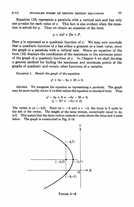
5-11] STANDARD FORMS OF SECOND DEGREE EQUATIONS 77
Equation (13) represents a parabola with a vertical axis and has onlyone i/-value for each value of x. This fact is also evident when the equa-tion is solved for y. Thus we obtain an equation of the form
y Ax* + Dx + F.
Here y is expressed as a quadratic function of x. We may now concludethat a quadratic function of x has either a greatest or a least value, since
the graph is a parabola with a vertical axis. Hence an equation of the
form (13) displays the coordinates of the maximum or the minimum pointof the graph of a quadratic function of x. In Chapter 6 we shall developa general method for finding the maximum and minimum points of the
graphs of quadratic and certain other functions of a variable.
EXAMPLE 1 . Sketch the graph of the equation
t/2 + Sx - 6</ + 25 = 0.
Solution. We recognize the equation as representing a parabola. The graph
may be more readily drawn if we first reduce the equation to standard form. Thus
2 - 60 + 9 = -8x - 25 + 9,
(y-
3)2 = -8(jr + 2).
The vertex is at (2,3). Since 4a = 8 and a = 2, the focus is 2 units to
the left of the vertex. The length of the latus rectum, numerically equal to 4a,
is 8. This means that the latus rectum extends 4 units above the focus and 4 units
below. The graph is constructed in Fig. 5-18.
FIGURE 5-18
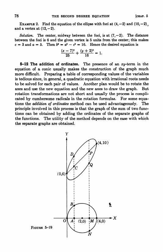
78 THE SECOND DEGREE EQUATION [CHAP. 5
EXAMPLE 2. Find the equation of the ellipse with foci at (4, 2) and (10, 2) f
and a vertex at (12, 2).
Solution. The center, midway between the foci, is at (7, 2). The distance
between the foci is 6 and the given vertex is 5 units from the center; this makes
c - 3 and a = 5. Then 62 = a2 c2 = 16. Hence the desired equation is
(x-
7)* (y + 2)*
25^
161.
6-12 The addition of ordinates. The presence of an zy-term in the
equation of a conic usually makes the construction of the graph muchmore difficult. Preparing a table of corresponding values of the variables
is tedious since, in general, a quadratic equation with irrational roots needs
to be solved for each pair of values. Another plan would be to rotate the
axes and use the new equation and the new axes to draw the graph. But
rotation transformations are not short and usually the process is compli-
cated by cumbersome radicals in the rotation formulas. For some equa-tions the addition of ordinates method can be used advantageously. The
principle involved in this process is that the graph of the sum of two func-
tions can be obtained by adding the ordinates of the separate graphs of
the functions. The utility of the method depends on the ease with which
the separate graphs are obtained.
FIGURE 5-19
D
(4,10)
5-13] IDENTIFICATION OF A CONIC 79
EXAMPLE. Draw the graph of the equation
2x* - 2xy + i/2 + 8z - I2y + 36 = 0.
Solution. To express y as the sum of two functions of x, we treat the equation
as a quadratic in y. Thus we have
/y2 + (-2* - 12)y + (2r> + 8* + 36) =
0,
and solving for y gives
2* + 12 db V(-2x -12)2- 4(2x* + 8s + 36) , Ay = _ = a; + 6
We now draw the graphs of the equations
y = x + 6 and y = V4x x2.
The locus of the first equation is a line. By squaring and then completing the
square in the z-terms, the second equation becomes (x 2)2 + j/
2 = 4. The
graph is a circle of radius 2 and center at (2,0). The line and circle are drawn in
Fig. 5-19. The point D on the graph of the given equation is obtained by adding
the ordinates AB and AC. That is, AC is extended by a length equal to AB.
The addition of ordinates for this purpose must be algebraic. Thus MN is nega-
tive and the point Q is found by measuring downward from P so that PQ = MN.By plotting a sufficient number of points in this manner the desired graph can be
drawn.
The graph, obtained from a second degree equation, is by definition a conic.
From the shape we conclude that the given equation represents an ellipse. In the
following section we show that this conclusion can be drawn immediately from
the equation itself.
6-13 Identification of a conic. The kind of conic represented by an
equation of the form
Ax* + Bxy + Cy* + Dx + Ey + F -
can be determined immediately from the coefficients of the second degree
terms. We already know how to identify the type of conic if B = 0. If
B 7* 0, we rotate the axes through an angle B (Section 4-4) and obtain
A'z'2 + B'x'ij' + C'y'* + D'x' + E'y' + F' -0,
where
A' - A cos2 B + B sin cos 6 + C sin2 6,
B' =$cos 26 - (A-
C) sin 26,
C' = A sin2 6 - B sin B cos + C cos2 0.
If B'2 - 4A /C" is computed, the result, when simplified, is
This relation among the coefficients of the original equation and the trans-
formed equation holds for any rotation. For this reason the expression

80 THE SECOND DEGREE EQUATION [CHAP. 5
B2 - 4AC is called an invariant. By selecting the particular rotation
for which B' = 0, we have
-44'C' = B2 - 1AC.
With B 1 - the kind of conic represented by the transformed equation,
and therefore the original equation, can be determined from the signs of
A' and C". The conic is an ellipse if A' and C" have like signs, and a
hyperbola if the signs are different. If either A' or C' is zero, the conic is
a parabola. These relations of A' and C", in the order named, would
make ~4A'C" negative, positive, or zero. Hence we have the following
important theorem.
THEOREM. The graph of Ax2 + Bxy + Cy* + Dx + Ey + F =0, when
it exists, is an ellipse, hyperbola, or a parabola according as B2 4AC is
negative, positive, or zero.
It must be remembered that in this theorem th.e degenerate conies
are included. These exceptional cases are indicated in the following
r6sum6:
B2 - 4AC < 0, ellipse or an isolated point,
B2 - 4AC > 0, hyperbola or two intersecting lines,
B2 - 44C =0, parabola, two parallel lines, or one line.
EXERCISE 5-4
In each problem 1-4 write the equation of the circle which satisfies the given
conditions.
1. Center (2,-6); radius 5. 2. Center (0,0); radius 3.
3. Center (0,4); radius 4. 4. Center (-2,0); radius 7.
5. The segment joining A(0,0) and B(8, 6) is a diameter.
6. The segment joining A( 5,1) and #(7,5) is a diameter.
Reduce the equations 7-10 to standard forms. Sketch the graph in each case
by the use of the vertex and the ends of the latus rectum.
7. y2 - I2x - 8y + 4 = 0. 8. z2 + I2x - 4.y + 36 = 0.
9. 4x2 + I2x - 16i/ + 41 = 0. 10. y*- Ix + 21 = 0.
Find the equations of the parabolas determined by the conditions given in
problems 11-14, Sketch each parabola.
11. Vertex (2,3); focus (5,3). 12. Vertex (-2,1); focus (-2,-!).
13. Vertex (0,2); axis vertical; length of latus rectum 16.
14. Vertex (-2,1); axis horizontal; passes through (0,-4).
Reduce equations 15-18 to standard forms. In each find the coordinates of
the center, the vertices, the foci, and the ends of the minor axis. Sketch each
curve.
6-13] IDENTIFICATION OF A CONIC 81
15. 16x2 + 25i/2 - 160z - 2(% + 400 = 0.
16. 9z2 + 25?/2 - 36z - 189 = 0.
17. 3*2 + 2i/2 - 24x + I2y + 60 = 0.
18. 4z2 + 8z/2 + 4x + 24y - 13 = 0.
Write the equation of the ellipse which satisfies the conditions in each prob-
lem 19-22. Sketch each ellipse.
19. Center (5,1); vertex (5,4); end of minor axis (3,1).
20. Vertex (6,3); foci (-4,3) and (4,3).
21. Ends of minor axis (-1,2) and (-l,-4); focus (-1,1).
22. Vertices (1,3) and (5,3); length of minor axis 4.
Reduce equations 23-26 to standard forms. In each find the coordinates of
the center, the vertices, and the foci. Describe the locus of each equation.
23. 9*2 -16*/
2 - 54x - 63 = 0.
24. 21x2 -4*/
2 + 84r - 32z/- 64 = 0.
25. 5?/2 - 4j2 -
30.y- 32z = 99.
26. 2//2 - 3x2 - 8y + fa - 1 = 0.
Write the equations of the hyperbolas which satisfy the conditions given in
problems 27-30.
27. Center (1,3); vertex (4,3); end of conjugate axis (1,1).
28. Vertex (-4,0); foci (-5,0) and (1,0).
29. Ends of conjugate axis (3, 1) and (3,5); focus (1,2).
30. Vertices (1,3) and (5,3); length of conjugate axis 6.
Sketch the graph of each equation 31-36 by the addition of ordinates method.
31. y = x Vj. 32. y = 6 - x V4 - z2.
33. y = 2x V5 + Qx - z2. 34. ?/
2 - 2xy + 2.r2 - 1 = 0.
35. *2 - 2xy + if- 4x - 12 = 0.
36. 2*2 + 2xy + if + Sx + 4y + 4 = 0.
Assuming that each equation 37-42 represents a nondegenerate conic, classify
each by computing I?2 4AC.
37. 2*2 - 4xy + 8y* + 7 = 0. 38. 3z2 + xy + x - 4 = 0.
39. 2jy-* + y-3 = 0. 40. z2 + 5xy + 15i/2 = 1.
41. x* - if + 4 = 0. 42. x2 -2xy + y* + 3x = 0.
43. 3x2 + Gxy + 3?/2 - x + y = 0. 44. 4z2 - toy + t/
2 + 13 = 0.
45. Determine whether the equation x2xy 2y* + x 2y = represents
a hyperbola or two intersecting lines by treating the equation as a quadratic in x
and solving for x in terms of y.
46. Solve the equation z2 + 2xy + ?/
2 2x 2y + 1 = for one variable in
terms of the other. Is the locus a parabola or a degenerate conic?
82 THE SECOND DEGREE EQUATION [CHAP. 5
47. Work out all the steps in showing that B" - 4A'C" * B2 - 4AC. Show
also that A' + C" = A + C.
Find the greatest or least value of each function 48 and 49. Draw the graph
and estimate the zeros of the function.
48. x2 - 7x + 4. 49. 5 - 2x - 2x\
50. Listening posts are at A, B, and C. Point A is 2000 feet north of point B,
and point C is 2000 feet east of B. The sound of a gun reaches A and B simul-
taneously one second after it reaches C. Show that the coordinates of the gun's
position are approximately (860,1000), where the z-axis passes through B and Cand the origin is midway between B and C. Assume that sound travels 1100 feet
per second.

CHAPTER 6
THE SLOPE OF A CURVE
6-1 An example. The graph of y = x* is shown in Fig. 6-1. Supposethat we draw a line through the point P(l,l) of the graph and a neigh-
boring point Q of the graph with abscissa 1 + h. The ordinate of Q, ob-
tained by replacing x by 1 + h in the equation, is (1 -I- h)*. Hence the
slope of the line is given by
m .
(14- h)-
\
The slope is thus expressed in terms of h. The quantity h may be assigned
any value except zero. This value is avoided because division by zero
is not permissible, and also because P and Q would then be the same point
and would not determine a line. Agreeing that h ^ 0, we substitute 1
for h/h in the expression for the slope, and have m = 2 4- h. While h must
not be zero, it may be as near zero as we please. A value of h near zero
makes the slope of the line through P and Q near 2. In fact, the slope
can be brought arbitrarily near 2 by taking h small enough. We see also
that when h is small Q is near P, and it can be made to take a position as
close to P as we please. Consider now the line through P with the slope 2
and denote the line by L. A line through P and Q can be obtained which
is arbitrarily near coincidence with L. This situation is described by say-
ing that as h approaches zero (or as Q approaches P) the line L is the limit-
FIGURE 6-1
83
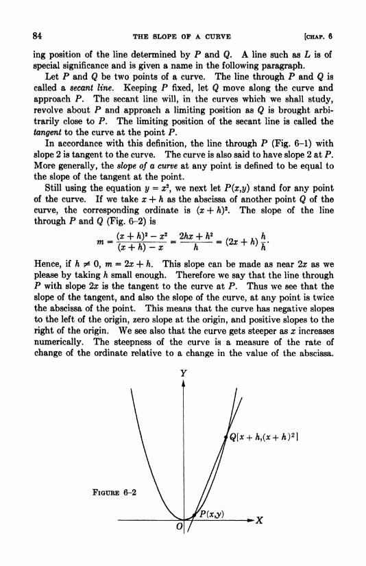
84 THE SLOPE OF A CURVE [CHAP. 6
ing position of the line determined by P and Q. A line such as L is of
special significance and is given a name in the following paragraph.Let P and Q be two points of a curve. The line through P and Q is
called a secant line. Keeping P fixed, let Q move along the curve and
approach P. The secant line will, in the curves which we shall study,
revolve about P and approach a limiting position as Q is brought arbi-
trarily close to P. The limiting position of the secant line is called the
tangent to the curve at the point P.
In accordance with this definition, the line through P (Fig. 6-1) with
slope 2 is tangent to the curve. The curve is also said to have slope 2 at P.
More generally, the slope of a curve at any point is defined to be equal to
the slope of the tangent at the point.
Still using the equation y = rr2
,we next let P(x,y) stand for any point
of the curve. If we take x + h as the abscissa of another point Q of the
curve, the corresponding ordinate is (x + h)2
. The slope of the line
through P and Q (Fig. 6-2) is
,A)
.
(x + K)- x h ' h
Hence, if h /* 0, m = 2x + h. This slope can be made as near 2x as we
please by taking h small enough. Therefore we say that the line throughP with slope 2x is the tangent to the curve at P. Thus we see that the
slope of the tangent, and also the slope of the curve, at any point is twice
the abscissa of the point. This means that the curve has negative slopes
to the left of the origin, zero slope at the origin, and positive slopes to the
right of the origin. We see also that the curve gets steeper as x increases
numerically. The steepness of the curve is a measure of the rate of
change of the ordinate relative to a change in the value of the abscissa.
FIGURE 6-2
6-3] THE DERIVATIVE 85
By means of the slope expression we gain considerable information about
the graph.
In this chapter we shall make use of the slope in studying the character-
istics of the graph of a function. This is a fundamental and powerful
concept of mathematics.
6-2 Limits. In the preceding example we observed that (2x + h)h/hcan be made arbitrarily close to 2x by taking h small. The expression 2x
is said to be the limit of the original expression as h approaches zero. Westate this fact symbolically as
lim (2x + h) \ = 2x.A-+O h
Although h approaches zero, we specify that it is not to be given the value
zero. This means that (2x + h)h/h is not equal to 2x, but can be madeas close as we please to 2x by choosing h small enough.
As a further illustration, we find the limit of
(x + h)*- x3
h
as h approaches zero. Here the result is not immediately evident. Thelimit can easily be found, however, if we first cube the binomial. Thus wehave
n
6-3 The derivative. Consider now the more general equation
-/(*>,
where the right member is some function of x. Let P and Q be two
points of the graph of the equation which have abscissas x and x + h.
The corresponding ordinates are f(x) and f(x + h). Hence the slope of the
line through P and Q (Fig. 6-3) is
f(x + h)-f(x) _f(x + h)-f(x)
(x + K)- x
The line through P with slope equal to

86 THE SLOPE OF A CURVE [CHAP. 6
FIGURE 6-3
is called the tangent to the curve at P. The slope of the curve at P is
defined to be the slope of the tangent.
The name derivative is given to the limit just mentioned, and Dxf(x) is
one notation for the limit or derivative. That is,
Other notations for the derivative of f(x) in y = f(x) are
dx' y', and -
dx
The derivative is a fundamental concept in calculus and has numerous
important applications. We shall make use of the derivative in the studyof a very restricted class of functions. A preliminary task in this con-
nection is the derivation of formulas by which the derivative of a func-
tion may be written at sight.
6-4 Derivative formulas. We first work out the derivative of axn,
where a is a constant and n is a positive integer. From the definition of
derivative,
~ ,. a(x + h)n axn
Dxaxn = lim -i--
To evaluate the limit, we expand (x + h)nby the binomial theorem, collect
like terms, and divide the numerator and denominator by h. Thus
a(x + h)n - axn a-- af
h \
x nx
= a
6-4] DERIVATIVE FORMULAS 87
The last expression has A as a factor in all terms except the first. Hencethe limit, as h approaches zero, of each term after the first is zero. Thelimit of the sum of these terms is also zero. Hence we have
Dxaxn = naxn~l. (1)
Notice that this formula permits us to write at once the derivative of a
constant times a positive integral power of x. We multiply by the expo-nent and decrease the power of x by one unit. In terms of slope, this
means that the graph of y = axn has at any point (x,y) the slope naxn~l.
If n =1, formula (1) becomes
Dxax = ar = a.
The derivative for this case is constant, as would be expected, since y = ax
is a straight line with the slope a.
Illustrations. D,5z3 = 15x2; D,(-2x4
)= -8z3
; D*z5 = 5x4
;Dx 3.
We next find the derivative of a constant. That is, we let
C.
where C is a constant. This means that f(x) has the same value for all
values of x, and therefore f(x + h) = C. Hence
h h h
Since h approaches zero but is not to assume the value zero, the quantity
0/ft is zero for all permissible values of h. We therefore conclude that
DXC = 0. (2)
This result is in agreement with what we would expect, because the
derivative is the slope of the graph of the function. The graph of f(x)= C
is a line parallel to the #-axis and the slope is zero at all its points.
An expression of the form
a<>xn + aix
n~ l + a2:rn-2
H-----h an-ix + an ,
where the a's are constants with a ^ 0, is a polynomial in x of the nth
degree. We now know how to write the derivative of each term of a
polynomial. The question then arises if the sum of the derivatives of the
separate terms is equal to the derivative of the sum of the terms. This
may be proved to be true. We shall make the assumption, omitting the
proof.
88 THE SLOPE OP A CURVE [CHAP. 6
We have established formula (1) for any positive integer n. In calculus
the formula is proved to hold for any real number n. We shall use the
formula for positive and negative integral exponents. The proof for a
negative integral exponent could be made by starting with the definition
of derivative and proceeding somewhat as in the case of a positive integral
exponent. We omit the proof, however.
EXAMPLE 1. Find the derivative of the polynomial
x* - 3^4 + 3.3_ 7a
. + 5.
Solution. To find the derivative, we apply formula (1) to each term containing
x and formula (2) to the constant term 5. Hence
3z4 + x3 - 7x + 5)= 20z4 - 12z3 + 3x2 - 7.
EXAMPLE 2. Write the derivative of 3or4 --H--- a: 3.or
1 x
Solution. We change the fractional terms to 5ar3 and x~ l and apply formu-
las (1) and (2). This gives
Dz(3ar4 - 5or3 + or 1 - x - 3) - -12*-' + l&r4 - x"2 - 1.
EXAMPLE 3. Find the slope of the curve
y = x3 - 3z2 + 4
at the point P(3,4). Write the equation of the tangent at this point.
Solution. We obtain the derivative (or slope expression) by using formulas (1)
and (2). ThusDxy = 3z2 - 6z.
The slope at the point P is obtained by substituting 3 for x in the derivative.
Hence the desired slope is 27 18 = 9. The equation of the line through (3,4)
with slope 9 is
9x - y- 23 = 0.
EXERCISE 6-1
Find the limits indicated in problems 1-6.
1. lim(z'-4). 2.. .--
x-*2 x->0 X + I
3. lim(2x-l). 4. Iim2(x +
+y-**. 6. Ii(-i-.-IH-h A-O \x + h xl h
Find/'(z) in each problem 7-20.
7. /(*) = 2x - 4. 8. /(x) - 5 - 6s.
9. /(*) = z3. 10. f(x) = 5*3
.
11. f(x) - 3x2 - 4*. 12. /(*) - z8 - 4x2 +13. /() = x-\ 14. /(x) - 5x- J + x.
15. /(x) - i-16.
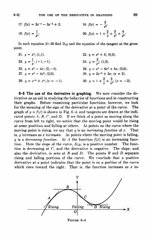
6-5)
17.
THE USE OF THE DERIVATIVE IN GRAPHING 89
= 3or4 - 5or2 + 2. 18. ~x
19. f(x) = ~
In each equation 21-30 find Dzy and the equation of the tangent at the given
point.
21.
23.
; (1,1). 22. t/= 3;(0,3).
25. y = x2 - 4x;(2,-4).
27. y = x4 - 4x2; (2,0).
29. ?/= x~4 + x4
; (x = -1).
24. y =; (1,3).
26. ?/= x3 - 6x2 + 8x; (0,0).
28. T/= 2x~2 + 3x; (x = 2).
30. y = 1 + ? +|;
(x = -2).
6-5 The use of the derivative in graphing. We now consider the de-
rivative as an aid in studying the behavior of functions and in constructing
their graphs. Before examining particular functions, however, we look
for the meaning of the sign of the derivative at a point of the curve. The
graph of //=
f(x) is shown in Fig. 0-4, and tangents are drawn at the indi-
cated points A , B, (\ and D. If we think of a point as moving along the
curve from left to right, we notice that the moving point would be rising
at some positions and falling at others. At points on the curve where the
moving point is rising, we say that y is an increasing Junction of x. That
is, y increases as x increases. At points where the moving point is falling,
y is a decreasing function. At .4 the function f(x) is an increasing func-
tion. Here the slope of the curve, Dxy, is a positive number. The func-
tion is decreasing at f, and the derivative is negative. The slope, and
also the derivative, is zero at B and D. The points B and D separate
rising and falling portions of the curve. We conclude that a positive
derivative at a point indicates that the point is on a portion of the curve
which rises toward the right. That is, the function increases as x in-

90 THE SLOPE OF A CURVE [CHAP. 6
creases. A negative derivative indicates a decreasing function; the curve
falls toward the right.
EXAMPLE 1. Find the values of x for which the graph of 5 + 4z x2 has
positive slopes, zero slope, or negative slopes.
Solution. We let y stand for the function and write
y = 5 + 4* - x\
For the derivative, we have
Dxy = 4 - 2x = 2(2-
z).
We note that the derivative is equal to zero when x = 2, is positive for x < 2,
and is negative for x > 2. That is,
Dxy > 0, when x < 2,
Dxy =0, when x =
2,
Dxy < 0, when x > 2.
Since the derivative expression gives the slope of the graph of the function,
we see that the graph has positive slopes to the left of x -2, zero slope at x =
2,
and negative slopes to the right of x = 2. This tells us that the curve is rising
at points to the left of x = 2 and falling at points to the right of x = 2. Hence
the graph has its greatest height at x 2. Substituting 2 for x in the given
function, we find the functional value, ?/, to be 9. Hence the point (2,9) is the
peak point of the graph, and 9 is the greatest value of the given function.
Noticing the derivative 2(2 x) further, we observe that at a point far to the
left of x = 2 the derivative is a large number, indicating that the curve is steep.
Similarly, the curve gets steeper and steeper as x increases beyond 2. The steep-
ness of the curve gives a measure of the rate of change in y relative to an increase
in x.
B(2,9)
FIGURE 6-5
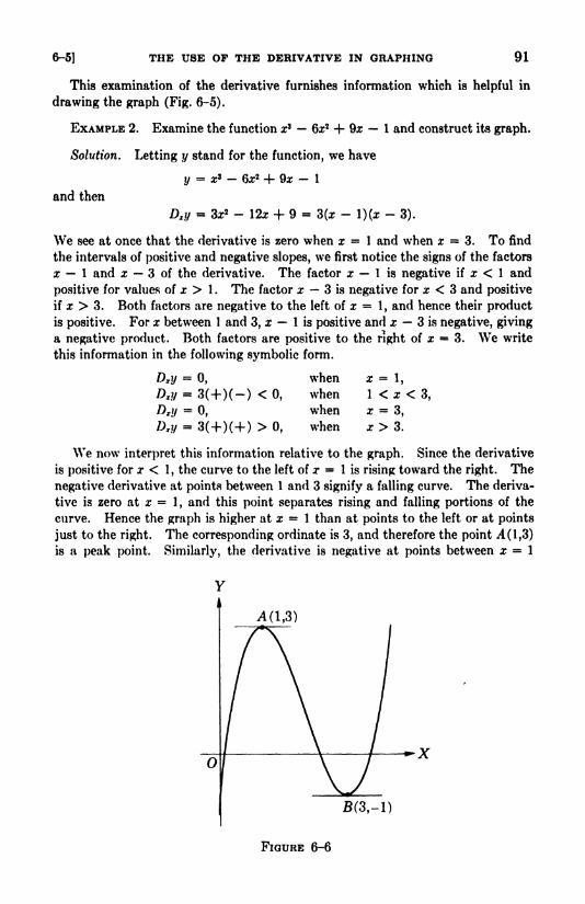
6-5] THE USE OP THE DERIVATIVE IN GRAPHING 91
This examination of the derivative furnishes information which is helpful in
drawing the graph (Fig. 6-5).
EXAMPLE 2. Examine the function x* 6x2 + 9z 1 and construct its graph.
Solution. Letting y stand for the function, we have
y = x9 6z2 + 9x 1
and then
Dxy- I2x + 9 -
3).
We see at once that the derivative is zero when x 1 and when x = 3. To find
the intervals of positive and negative slopes, we first notice the signs of the factors
x 1 and x 3 of the derivative. The factor x 1 is negative if x < I and
positive for values of x > 1 . The factor x 3 is negative for x < 3 and positive
if x > 3. Both factors are negative to the left of x =1, and hence their product
is positive. For x between 1 and 3, x 1 is positive and x 3 is negative, giving
a negative product. Both factors are positive to the right of x = 3. We write
this information in the following symbolic form.
Dxy =0, when x =
1,
Dxy = 3(+)(-) < 0, when 1 < x < 3,
Dxy =0, when x =
3,
Dxy = 3(+)(+ ) > 0, when x > 3.
We now interpret this information relative to the graph. Since the derivative
is positive for x < 1,the curve to the left of x = 1 is rising toward the right. The
negative derivative at points between 1 and 3 signify a falling curve. The deriva-
tive is zero at x = 1,and this point separates rising and falling portions of the
curve. Hence the graph is higher at x = 1 than at points to the left or at points
just to the right. The corresponding ordinate is 3, and therefore the point A (1,3)
is a peak point. Similarly, the derivative is negative at points between x = 1
FIGURE 6-6
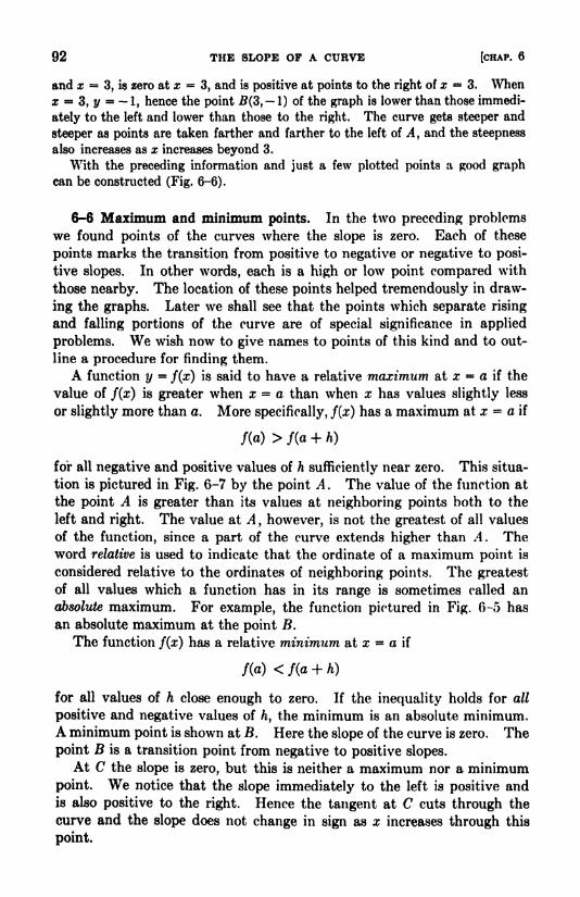
92 THE SLOPE OP A CURVE [CHAP. 6
and x = 3, is zero at x = 3, and is positive at points to the right of x = 3. Whenx =
3, y = 1, hence the point 5(3, 1) of the graph is lower than those immedi-
ately to the left and lower than those to the right. The curve gets steeper and
steeper as points are taken farther and farther to the left of A, and the steepness
also increases as x increases beyond 3.
With the preceding information and just a few plotted points a good graph
can be constructed (Fig. 6-6).
6-6 Maximum and minimum points. In the two preceding problemswe found points of the curves where the slope is zero. Each of these
points marks the transition from positive to negative or negative to posi-
tive slopes. In other words, each is a high or low point compared with
those nearby. The location of these points helped tremendously in draw-
ing the graphs. Later we shall see that the points which separate rising
and falling portions of the curve are of special significance in applied
problems. We wish now to give names to points of this kind and to out-
line a procedure for finding them.
A function y = f(x) is said to have a relative maximum at x = a if the
value of f(x) is greater when x = a than when x has values slightly less
or slightly more than a. More specifically, f(x) has a maximum at x = a if
f(a)>f(a + h)
for all negative and positive values of h sufficiently near zero. This situa-
tion is pictured in Fig. 6-7 by the point A . The value of the function at
the point A is greater than its values at neighboring points both to the
left and right. The value at A, however, is not the greatest of all values
of the function, since a part of the curve extends higher than A. Theword relative is used to indicate that the ordinate of a maximum point is
considered relative to the ordinates of neighboring points. The greatest
of all values which a function has in its range is sometimes called an
absolute maximum. For example, the function pictured in Fig. 6-5 has
an absolute maximum at the point B.
The function f(x) has a relative minimum at x = a if
/(a) <f(a + h)
for all values of h close enough to zero. If the inequality holds for all
positive and negative values of ft, the minimum is an absolute minimum.A minimum point is shown at JB. Here the slope of the curve is zero. The
point B is a transition point from negative to positive slopes.
At C the slope is zero, but this is neither a maximum nor a minimumpoint. We notice that the slope immediately to the left is positive andis also positive to the right. Hence the tangent at C cuts through the
curve and the slope does not change in sign as x increases through this
point.
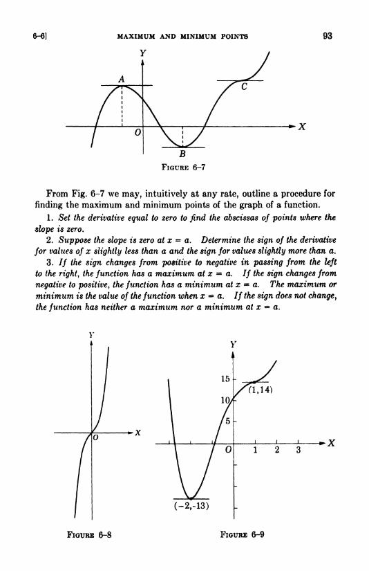
6-6] MAXIMUM AND MINIMUM POINTS
Y
93
\\L/
BFIGURE 6-7
From Fig. 6-7 we may, intuitively at any rate, outline a procedure for
finding the maximum and minimum points of the graph of a function.
1. Set the derivative equal to zero to find the abscissas of points where the
slope is zero.
2. Suppose the slope is zero atx-a. Determine the sign of the derivative
for values of x slightly less than a and the sign for values slightly more than a.
3. // the sign changes from positive to negative in passing from the left
to the right, the function has a maximum at x = a. If the sign changes from
negative to positive, the function has a minimum at x - a. The maximum or
minimum is the value of the function when x - a. If the sign does not change,
the function has neither a maximum nor a minimum at x - a.
FIGURE 6-8 FIGURE 6-9
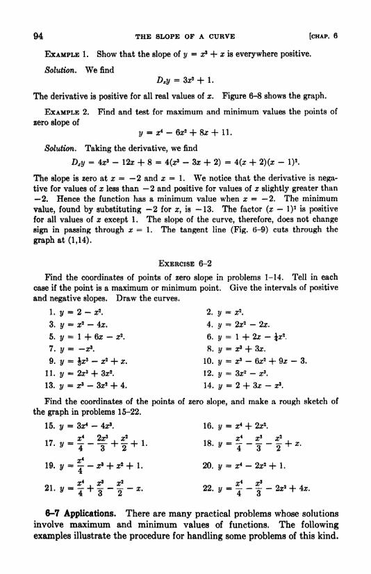
94 THE SLOPE OP A CURVE [CHAP. 6
EXAMPLE 1. Show that the slope of y = x3 + x is everywhere positive.
Solution. We find
Dxy - 3x2 + 1.
The derivative is positive for all real values of x. Figure 6-8 shows the graph.
EXAMPLE 2. Find and test for maximum and minimum values the points of
zero slope of
y = x4 -6x2 + 8x + 11.
Solution. Taking the derivative, we find
Dxy = 4x3 - 12x + 8 = 4(x3 - 3x + 2)
= 4(x + 2)(x-
I)2
.
The slope is zero at x = 2 and x = 1. We notice that the derivative is nega-
tive for values of x less than 2 and positive for values of x slightly greater than
2. Hence the function has a minimum value when x = 2. The minimum
value, found by substituting 2 for x, is 13. The factor (x I)2 is positive
for all values of x except 1. The slope of the curve, therefore, does not change
sign in passing through x = 1. The tangent line (Fig. 6-9) cuts through the
graph at (1,14).
EXERCISE 6-2
Find the coordinates of points of zero slope in problems 1-14. Tell in each
case if the point is a maximum or minimum point. Give the intervals of positive
and negative slopes. Draw the curves.
1. y = 2 - x2. 2. y = x2
.
3. y = x2 - 4x. 4. y = 2x2 - 2x.
5. y = 1 + 6x - x2. 6. y = 1 + 2x - ix
2.
7. y = -x3. 8. y = x3 + 3x.
9. y = Jx3 - x2 + x. 10. y = x3 - 6x2 + 9x - 3.
11. y = 2x3 + 3x2. 12. y = 3x2 - x3
.
13. y = x3 - 3x2 + 4. 14. y = 2 + 3x - x3.
Find the coordinates of the points of zero slope, and make a rough sketch of
the graph in problems 15-22.
15. y = 3x4 - 4x3. 16. y = x4 + 2x2
.
_ x4 2x3 x2, 1 10 x4 x3 x2
". y - T- T +
2+ 1. ^ y - T
"3-
2+ *
19. y = - x8 + x2 + 1. 20. y = x4 - 2x2 + 1.
6-7 Applications. There are many practical problems whose solutions
involve maximum and minimum values of functions. The following
examples illustrate the procedure for handling some problems of this kind.
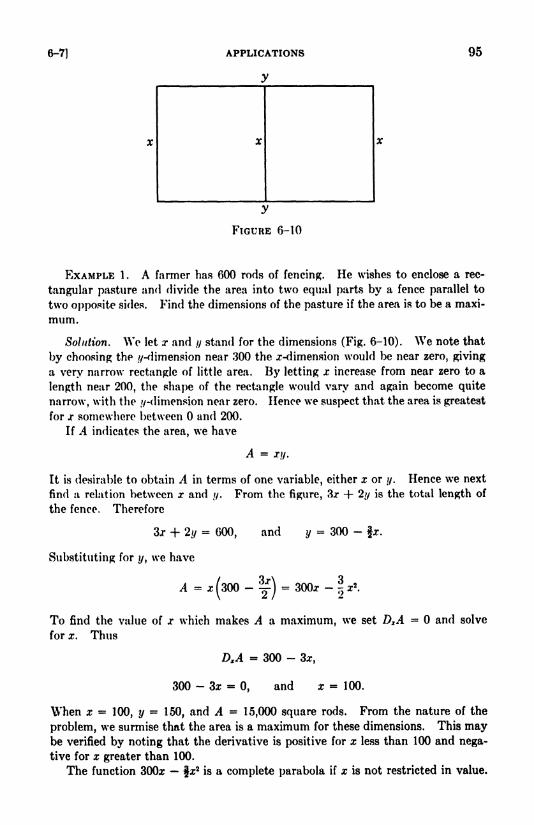
6-7] APPLICATIONS
y
95
FIGURE 6-10
EXAMPLE 1. A farmer has 600 rods of fencing. He wishes to enclose a rec-
tangular pasture and divide the area into two equal parts by a fence parallel to
two opposite sides. Find the dimensions of the pasture if the area is to be a maxi-
mum.
Solution. Wo let x and // stand for the dimensions (Fig. 6-10). We note that
by choosing the //-dimension near 300 the x-dimension would be near zero, giving
a very narrow rectangle of little area. By letting x increase from near zero to a
length near 200, the shape of the rectangle would vary and again become quite
narrow, with the //-dimension near zero. Hence we suspect that the area is greatest
for jc somewhere between and 200.
If .4 indicates the area, we have
A = xy.
It is desirable to obtain A in terms of one variable, either x or ?/. Hence we next
find a relation between x and //. From the figure, 3r 4- 2y is the total length of
the fence. Therefore
3x + 2//= 600, and y = 300 - $x.
Substituting for ?/, we have
A = x(300
-y)
= 300* - I x2.
To find the value of x which makes A a maximum, we set DZA = and solve
for x. Thus
DtA = 300 - 3*,
300 - 3x =0, and x = 100.
When x = 100, y = 150, and A = 15,000 square rods. From the nature of the
problem, we surmise that the area is a maximum for these dimensions. This maybe verified by noting that the derivative is positive for x less than 100 and nega-
tive for x greater than 100.
The function 300x - fx2
is a complete parabola if x is not restricted in value.
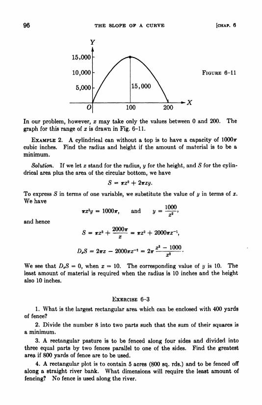
96 THE SLOPE OP A CURVE [CHAP. 6
FIGURE 6-11
100 200
In our problem, however, x may take only the values between and 200. The
graph for this range of x is drawn in Fig. 6-11.
EXAMPLE 2. A cylindrical can without a top is to have a capacity of lOOOir
cubic inches. Find the radius and height if the amount of material is to be a
minimum.
Solution. If we let x stand for the radius, y for the height, and S for the cylin-
drical area plus the area of the circular bottom, we have
S = Trz2 + 2*xy.
To express S in terms of one variable, we substitute the value of y in terms of x.
We have
wty =10007T, and y = ^,
and hence
20007T
DXS = 2wx -- 1000
We see that DZS 0, when x = 10. The corresponding value of \j is 10. The
least amount of material is required when the radius is 10 inches and the height
also 10 inches.
EXERCISE 6-3
1. What is the largest rectangular area which can be enclosed with 400 yardsof fence?
2. Divide the number 8 into two parts such that the sum of their squares is
a minimum.
3. A rectangular pasture is to be fenced along four sides and divided into
three equal parts by two fences parallel to one of the sides. Find the greatest
area if 800 yards of fence are to be used.
4. A rectangular plot is to contain 5 acres (800 sq. rds.) and to be fenced off
along a straight river bank. What dimensions will require the least amount of
fencing? No fence is used along the river.
6-7] APPLICATIONS 97
5. A rectangular box is to be made from a sheet of tin 8 inches by 12 inches
by cutting square pieces from each corner and then turning up the sides. For
what depth will the volume of the box be a maximum?
6. A box with a square base and open top is to be made from 27 square feet
of material. Find the dimensions if the volume is to be a maximum.
7. An uncovered rectangular water tank is to be lined with sheet copper. If
the tank is to hold 108 cubic feet of water and the base is a square, find the dimen-
sions for a minimum amount of sheet copper.
S. A closed cylindrical can is to be made from 24ir square inches of sheet tin.
Find the radius and height in order for the volume to be a maximum.
0. A closed cylindrical can is to be made to contain 16?r cubic inches. Whatshould bo the radius and height for the amount of tin to be a minimum?
10. A window is formed by a rectangle surmounted by a semicircle and has a
perimeter of 12 foot. Find the dimensions to admit the most light.
1 1 . The combined length and girth of a parcel post package must not exceed
100 inches. What is the volume of the largest box with a square base that can
be sent by parcel post?
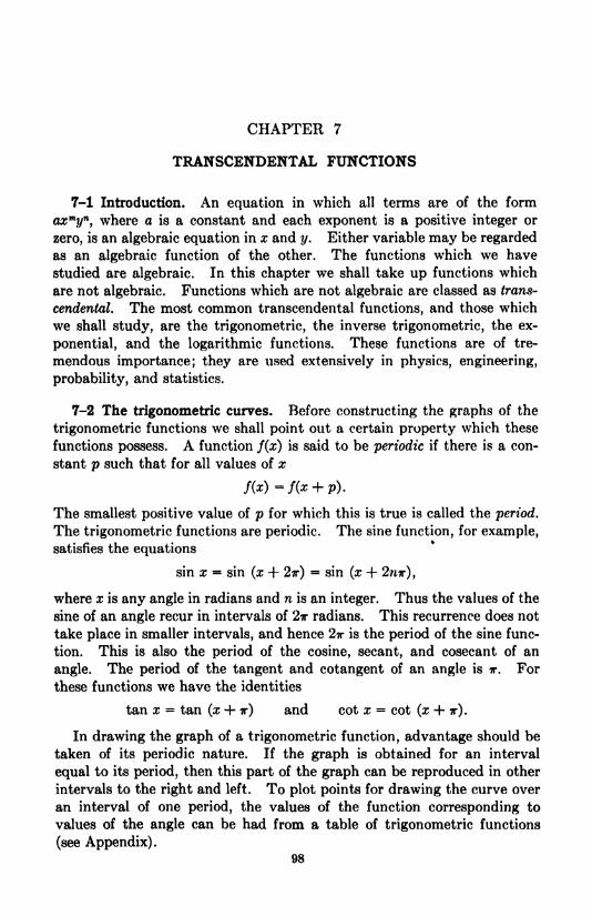
CHAPTER 7
TRANSCENDENTAL FUNCTIONS
7-1 Introduction. An equation in which all terms are of the form
axmyn
,where a is a constant and each exponent is a positive integer or
zero, is an algebraic equation in x and y. Either variable may be regarded
as an algebraic function of the other. The functions which we have
studied are algebraic. In this chapter we shall take up functions which
are not algebraic. Functions which are not algebraic are classed as trans-
cendental. The most common transcendental functions, and those which
we shall study, are the trigonometric, the inverse trigonometric, the ex-
ponential, and the logarithmic functions. These functions are of tre-
mendous importance; they are used extensively in physics, engineering,
probability, and statistics.
7-2 The trigonometric curves. Before constructing the graphs of the
trigonometric functions we shall point out a certain property which these
functions possess. A function f(x) is said to be periodic if there is a con-
stant p such that for all values of x
/(*)-/(* + ?).
The smallest positive value of p for which this is true is called the period.
The trigonometric functions are periodic. The sine function, for example,satisfies the equations
sin x = sin (x + 2-ir)= sin (x + 2n?r),
where x is any angle in radians and n is an integer. Thus the values of the
sine of an angle recur in intervals of 2w radians. This recurrence does not
take place in smaller intervals, and hence 2ir is the period of the sine func-
tion. This is also the period of the cosine, secant, and cosecant of an
angle. The period of the tangent and cotangent of an angle is TT. For
these functions we have the identities
tan x = tan (x + TT) and cot x = cot (x + IT).
In drawing the graph of a trigonometric function, advantage should be
taken of its periodic nature. If the graph is obtained for an interval
equal to its period, then this part of the graph can be reproduced in other
intervals to the right and left. To plot points for drawing the curve over
an interval of one period, the values of the function corresponding to
values of the angle can be had from a table of trigonometric functions
(see Appendix).98
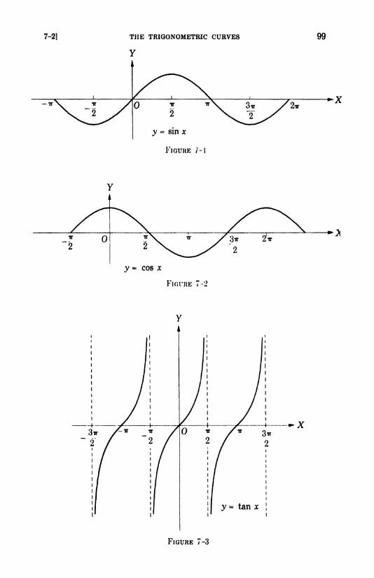
7-2] THE TRIGONOMETRIC CURVES
Y
IT
2
y = sin x
FIGURE 7-1
y = cos x
FIGURE 7-2
FIGURE 7-3

100 TRANSCENDENTAL FUNCTIONS [CHAP. 7
Figures 7-1 and 7-2 show the graphs of y = sin x and y = cos x. Each
of these curves crosses the x-axis after every IT radians of re-values. Theordinates of each vary from 1 to 1. These are called the extreme values,
and the constant 1 is called the amplitude.
The tangent curve (Fig. 7-3) crosses the avaxis at integral multiples of
v radians and has asymptotes at odd integral multiples of T radians.
Amplitude is not defined for the tangent.
The secant curve (Fig. 7-4) has no x-intercepts. The asymptotes occur
after every TT radians of z-values.
We next consider the function a sin bx, where a and b are constants.
Since the extreme values of sin bx are 1 and 1, the extreme values of
a sin bx are a and a. The amplitude is equal to the absolute value of a.
To find the period, we determine how much x changes in producing a
O
y = sec x
FIGURE 7-4
y = 3 sin 2x
FIGURE 7-5
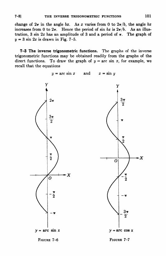
7-3] THE INVERSE TRIGONOMETRIC FUNCTIONS 101
change of 2v in the angle bx. As x varies from to 2ir/6, the angle bx
increases from to 2ir. Hence the period of sin bx is 2-ir/b. As an illus-
tration, 3 sin 2x has an amplitude of 3 and a period of TT. The graph of
y = 3 sin 2x is drawn in Fig. 7-5.
7-3 The inverse trigonometric functions. The graphs of the inverse
trigonometric functions may be obtained readily from the graphs of the
direct functions. To draw the graph of y = arc sin z, for example, werecall that the equations
y arc sin x and x = sin y
y - arc sin x
FIGURE 7-6
y arc cos x
FIGURE 7-7

102 TRANSCENDENTAL FUNCTIONS
Y
STT
[CHAP 7
FIGURE 7-8
express the same relation between x and y. Hence the graphs of these
two equations must coincide. The equations
x = sin y and y = sin x
have x and y interchanged. The graph of y = sin x (Fig. 7-1) winds
along the or-axis. We conclude, therefore, that the graph of x = sin y
is a curve of the same form winding along the ?/-axis. The graph of
x = sin T/, or y = arc sin x, is shown in Fig. 7-6.
The graphs of each of the other inverse functions can be found similarly
from the graph of the direct function by reversing the roles of x and y.
Figures 7-7 and 7-8 show the graphs of y = arc cos x and y = arc tan x.
EXERCISE 7-1
Find the period of each function 1-12. Give the amplitudes of the sine and
cosine functions.
1. cosSx.
4. 2 cos 4x.
7. secGx.
10. SCOSTTX.
2. sinjx.
5. tan 5x.
8. cos7x.
11.
3. sinjz.
6. cot is.
9. tanfz.
12. sec (is +

7-4] THE EXPONENTIAL CURVES 103
Sketch the graph of each equation 13-24.
13. //= 3 cos x. 14. y = 2 sin x.
16. u = cos2x. 17. y = tan 2x.
19. //= 3 sin x. 20. //
= 4 tan j.
22. //= tan Jx. 23. //
= esc x.
15. y = sin 3z.
IS. y = cot a:.
21. y + 4 sin fa;.
24. y = 5 sin 4z.
Draw the graphs of the inverse trigonometric equations 25-30.
25. //= 2 arc cos X. 26. y = 3 arc sin x.
27. //= 2 arc tan x. 28. ?/
= J arc cos ^x.
29. //= 3 arc sin %x. 30. y = arc tan 2x.
7-4 The exponential curves. An equation in which a variable or a
function of a variable is an exponent is called an exponential equation. The
corresponding graph is known as an exponential curve. The equations
and = 10'
are simple exponential equations. Each could be made more general byreplacing the exponent by a less simple function of x.
The letter c in the second equation stands for an irrational number
approximately equal to 2.71828. This number is of great importance in
FIGURE 7-9
104 TRANSCENDENTAL FUNCTIONS [CHAP. 7
advanced mathematics, and exponential functions involving e as a base
have wide applications in both theory and practice.
The graph of y = e* can be drawn by using the table (see Appendix) to
find values of y for assigned values of or. Corresponding values of y in
the equations y = 2J and y = 10X are simply obtained when x is an integer.
To determine other pairs of values a table of logarithms can be used.
Figure 7-9 has the graph of the three equations drawn in the same coordi-
nate system for purposes of comparison.
7-5 Logarithmic curves. If a is a positive number different from 1 and
y is any real number in the equation av = z, then y is called the logarithm
of x to the base a. This relation may be written symbolically as y = loga x.
Thus the two equations
and y = loga xa* = x
express the same relation among the numbers a, ,and y. The first is in
exponential form and the second in logarithmic form. Since the base a is
positive, av also has a positive value. Hence we shall consider the loga-
rithms of positive numbers only.
Since a logarithmic equation can be changed to an exponential equa-
tion, it appears that logarithmic and exponential curves must be closely
related. To see the relation, we note that the logarithmic equation
y = logfl x is equivalent to, and therefore has the same graph as, x = av.
Now the equations
x = av and y = a*
are alike except that x and y play reverse roles. Hence their graphs must
have the same form but different positions relative to the coordinate axes.
/7\ 2345678
FIGURE 7-10

7-6] THE GRAPH OF THE SUM OF TWO FUNCTIONS 105
The most frequently used bases for logarithms are the numbers 10 and e.
A table of logarithms can be used for drawing the curve corresponding to a
logarithmic equation employing either of these bases. Corresponding
values of x and y for the equations y = log x and y = log,, x are here tabu-
lated with the logarithmic values rounded off to one decimal place. These
should be verified by referring to the tables in the Appendix. The graphsare drawn in Fig. 7-10.
EXERCISE 7-2
Sketch the graphs of the following equations:
1. y = 4'.
4. y = e2*.
7. //= 22*-'.
10. //= 3 logm x.
12. //= Iog 10 (-.r).
14. //=
log, 4.r.
16. //= logo j.
2. y = 4-'. 3. y = 2e*.
5. //= c
r'. 6. y = (>'**.
8. y = 2*2~*. 9. y = are*.
11. //= 2 log,*.
13. y = logc (-j).
15. y =log,, a-
2.
17. //= Iog10 (:r
-3).
18. Show that the graph of //= loga bx is the graph of //
= loga x shifted verti-
cally a distance of log,, b.
19. Show that the graph of //=
log,, x2 can be obtained by doubling each ordi-
nate of ?/= loga j.
20. If S100 is invested at 2% per year compounded continuously, the accumu-
lated amount // at the end of x years is given by the equation
y = lOOe002*.
Sketch the graph of this equation and from the graph estimate the accumulated
amount at the end of (a) 3 years, (b) 6 years, (c) 9 years. Estimate also the
time required for the original investment to double.
7-6 The graph of the sum of two functions. The addition of ordinates
method can sometimes be efficiently applied to draw the graph of the sumof two functions in which one or both are transcendental. The process is
exactly that used in Section 5-12 and is illustrated by the following example
involving a transcendental function,
EXAMPLE 1. Sketch the graph of the equation
y = Vx + sin x.
Solution. We first draw the graphs of
y Vx, and y = sin x.
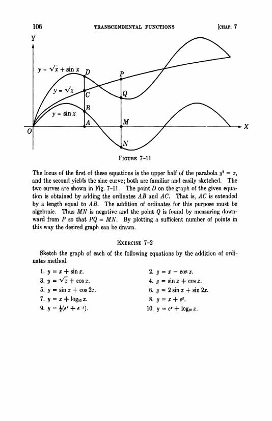
TRANSCENDENTAL FUNCTIONS [CHAP. 7
FIGURE 7-11
The locus of the first of these equations is the upper half of the parabola ?/
2 =x,
and the second yields the sine curve; both are familiar and easily sketched. The
two curves are shown in Fig. 7-11. The point D on the graph of the given equa-
tion is obtained by adding the ordinates AB and AC. That is, AC is extended
by a length equal to AB. The addition of ordinates for this purpose must be
algebraic. Thus MN is negative and the point Q is found by measuring down-
ward from P so that PQ = MN. By plotting a sufficient number of points in
this way the desired graph can be drawn.
EXERCISE 7-2
Sketch the graph of each of the following equations by the addition of ordi-
nates method.
1. y = x + sin a-.
3. y = Vx + cos x.
5. y = sin x + cos 2ar.
7. y = x + logic x.
9. y =i(e* + e~x).
2. y= x cos x.
4. y= sin x + cos x.
6. y= 2 sin x + sin 2x.
8. y = x + e*.
10. y = e' + logio x.

CHAPTER 8
EQUATIONS OF CURVES AND CURVE FITTING
8-1 Equation of a given curve. Having obtained curves as the graphsof equations, it is natural to surmise that a curve in a plane has a corre-
sponding equation. We shall first consider the problem of writing the
equation of a curve all of whose points are definitely fixed by certain given
geometric conditions. The graph of the resulting equation should be
in exact agreement with the given curve. In other words, the equationof a curve is a relation between x and y which is satisfied by the coordi-
nates of all points, and only those points, which belong to the given curve.
In the latter part of this chapter we shall consider the problem of find-
ing the equation when the original information locates certain points
(usually a few) but does not establish any particular curve.
EXAMPLE 1. A point moves so that its distance from the fixed point F(2,Q)divided by its distance from the //-axis is always equal to J. Find the equationof the locus of the moving point.
Solution. We select a typical point P of the path (Fig. 8-1). Then 2FI> = DPexpresses the required relation between the distances. In terms of the coordinates
jc and // of the variable point P, this relation is
or, by simplification,
2\ (x-
2)* -f //'
4y/'- Iftr + 16 = 0.
This is the equation of an ellipse, since .r2 and //- have unequal coefficients of the
same sign.
Y
D
O F(2,0)
FIGURE 8-1
107

108 EQUATIONS OF CURVES AND CURVE FITTING [cHAP. 8
EXAMPLE 2. Find the equation of the circle which passes through the points
(-2,-2), (5,-3),and(2,l).
Solution. The equation of the circle can be written in the form
s* + y* + Dx + Ey + F = 0.
Our problem is to find values for D, E, and F so that this equation is satisfied bythe coordinates of the given points. Hence we substitute for x and y the coordi-
nates of these points. This gives the system
4 + 4 _ 2D - 2E + F =0,
25 + 9 + 5D - 3E + F =0,
4+l + 2D + + P = 0.
The solution of these equations is D =3, E =
5, and F = 4. Therefore the
required equation is
x* + y*- 3x + 5y - 4 = 0.
EXERCISE 8-1
In each problem 1-14 find the equation of the locus of P(x,y) which satisfies
the given condition.
1. P is 5 units from the fixed point (2, 3).
2. P is equidistant from (2, -4) and (-1,5).
3. The abscissa of P is equal to its distance from the point (3,2).
4. P is on the circle with center at (3, 2) and which passes through (6,2).
5. P is the vertex of a right triangle whose hypotenuse is the segment joining
(-5,0) and (5,0).
6. The sum of the squares of the distances between P and the points (4,2)
and (-3,1) is 50.
7. P is twice as far from (0,3) as from (3,0).
8. P is three times as far from (1,1) as from (3,4).
9. P is equidistant from (8,1) and the ly-axis.
10. P is twice as far from the x-axis as from (0,3).
11. P is twice as far from (5,0) as from the y-axis.
12. The sum of the distances from P to (0,-3) and to (0,3) is 10.
13. The difference of the distances from P to ( 5,0) and to (5,0) is numerically
equal to 8.
14. The angle APB = 45, where A and B are the points (-1,0) and (1,0).
15. A point moves so that its distance from a fixed point divided by its dis-
tance from a fixed line is always equal to a constant e. Find the equation of the
path of the moving point. Suggestion: Take the y-axis along the fixed line andthe z-axis through the fixed point, say (fc,0). From the resulting equation observe
that the path is a parabola if e = 1, ati ellipse if e is between zero and 1, and a
hyperbola if e is greater than 1. Show that for e * 1 the z-intercepts (vertices)
are k/(\ + e) and k/(l-
e). Where is the center of the conic? Divide the dis-
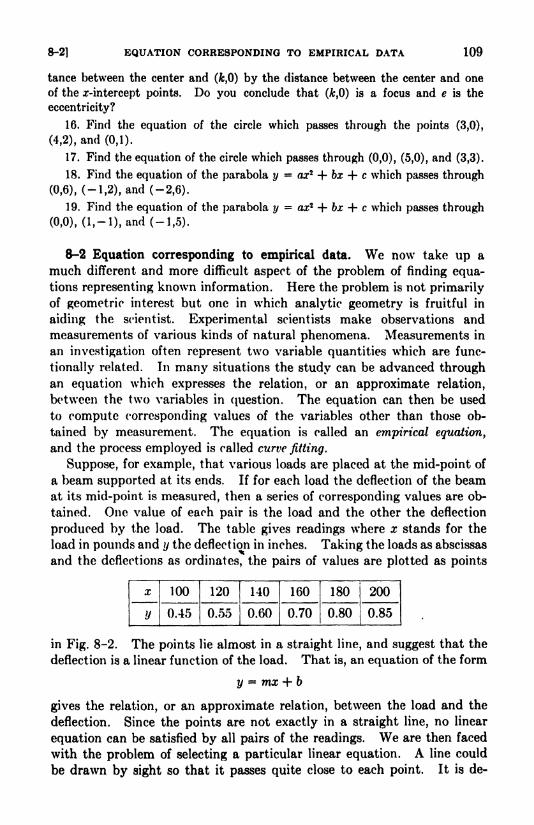
8-2] EQUATION CORRESPONDING TO EMPIRICAL DATA 109
tance between the center and (fc,0) by the distance between the center and one
of the z-intercept points. Do you conclude that (A;,0) is a focus and e is the
eccentricity?
16. Find the equation of the circle which passes through the points (3,0),
(4,2), and (0,1).
17. Find the equation of the circle which passes through (0,0), (5,0), and (3,3).
18. Find the equation of the parabola y = ax2 + bx + c which passes through
(0,6), (-1,2), and (-2,6).
19. Find the equation of the parabola y- ax2 + bx + c which passes through
(0,0), (l,-l),and(-l,5).
8-2 Equation corresponding to empirical data. We now take up a
much different and more difficult aspect of the problem of finding equa-tions representing known information. Here the problem is not primarily
of geometric interest but one in which analytic geometry is fruitful in
aiding the scientist. Experimental scientists make observations and
measurements of various kinds of natural phenomena. Measurements in
an investigation often represent two variable quantities which are func-
tionally related. In many situations the study can be advanced throughan equation which expresses the relation, or an approximate relation,
between the two variables in question. The equation can then be used
to compute corresponding values of the variables other than those ob-
tained by measurement. The equation is called an empirical equation,
and the process employed is called curve fitting.
Suppose, for example, that various loads are placed at the mid-point of
a beam supported at its ends. If for each load the deflection of the beamat its mid-point is measured, then a series of corresponding values are ob-
tained. One value of each pair is the load and the other the deflection
produced by the load. The table gives readings where x stands for the
load in pounds and y the deflection in inches. Taking the loads as abscissas
and the deflections as ordinates, the pairs of values are plotted as points
in Fig. 8-2. The points lie almost in a straight line, and suggest that the
deflection is a linear function of the load. That is, an equation of the form
y = mx + b
gives the relation, or an approximate relation, between the load and the
deflection. Since the points are not exactly in a straight line, no linear
equation can be satisfied by all pairs of the readings. We are then faced
with the problem of selecting a particular linear equation. A line could
be drawn by sight so that it passes quite close to each point. It is de-
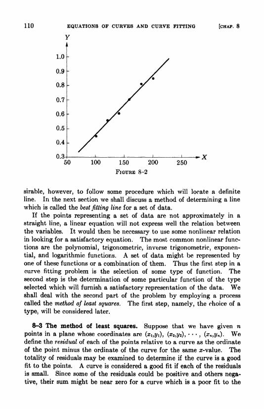
110 EQUATIONS OP CURVES AND CURVE FITTING
Y
[CHAP. 8
100 150 200
FIGURE 8-2
250
sirable, however, to follow some procedure which will locate a definite
line. In the next section we shall discuss a method of determining a line
which is called the best fitting line for a set of data.
If the points representing a set of data are not approximately in a
straight line, a linear equation will not express well the relation between
the variables. It would then be necessary to use some nonlinear relation
in looking for a satisfactory equation. The most common nonlinear func-
tions are the polynomial, trigonometric, inverse trigonometric, exponen-
tial, and logarithmic functions. A set of data might be represented byone of these functions or a combination of them. Thus the first step in a
curve fitting problem is the selection of some type of function. Thesecond step is the determination of some particular function of the typeselected which will furnish a satisfactory representation of the data. Weshall deal with the second part of the problem by employing a processcalled the method of least squares. The first step, namely, the choice of a
type, will be considered later.
8-3 The method of least squares. Suppose that we have given n
points in a plane whose coordinates are (zi,2/i), (#2,2/2), , (#n,2/n). Wedefine the residual of each of the points relative to a curve as the ordinate
of the point minus the ordinate of the curve for the same z-value. The
totality of residuals may be examined to determine if the curve is a goodfit to the points. A curve is considered a good fit if each of the residuals
is small. Since some of the residuals could be positive and others nega-
tive, their sum might be near zero for a curve which is a poor fit to the

8-3] THE METHOD OF LEAST SQUARES 111
points. Hence the sum of the residuals would not furnish a reliable
measure of the accuracy of fit. For this reason we shall deal with the
squares of the residuals, thus avoiding negative quantities. If the sumof the squares of the residuals is small, we would know that the curve
passes close to each of the n points. The better fitting of two curves
of the same type is the one for which the sum of the squares of the residuals
is smaller. The best fitting curve of a given type is the one for which the
sum of the squares of the residuals is a minimum.
Starting with the simplest situation, we shall show how to determine
the best fitting line to the n given points. We write the linear equation
?/= mx + 6,
where values are to be found for m and b so that the sum of the squares
of the residuals of the n points is a minimum. The residual of the point
(ri,.Vi) is //i (mx\ + fo). The quantity y\ is the ordinate of the point,
and (mx\ + b) is the ordinate of the line when x = XL Hence the residuals
of the points are
+ 6), ?/2-
(tt?:r2 + 6), , ?/- (mxn + 6),
and their squares are
/i2 -
//22 -
2/WJ2//2-
2//2& + w?W + 2m.r26 + 62,
//n2 - 2mxn ijn
-2//n6 + m 2xn
2 + 2mxnfc + b2.
To express the sum of these expressions in a convenient form, we use
the following notation.
J2//2 H-----H XnUn-
Denoting the sum of the squares of the residuals by /?, we have
R = iy - 2m2xy - 2b2y + m*2x2 + 2mb2x + n62.
We notice that all quantities in /? are fixed except m and b. For example,
2/y2is not a variable; it stands for the sum of the squares of the ordinates
of the n fixed points.
Our problem now is to determine values for m and b which make R a
minimum. The expression for R contains the first and second powers of
both m and b. If 6 is assigned any value whatever, then R is a quadratic
function of m. Hence the graph of the function is a parabola. Choosing
the m-axis as horizontal and treating b as an unspecified constant, the
parabola has a vertical axis and extends upward. The parabola opens
upward because /?, being the sum of squared expressions, is not negative.
112 EQUATIONS OF CURVES AND CURVE FITTING [CHAP. 8
Consequently the least value of R is the ordinate of the vertex. If weset ra equal to its value at the vertex, a relation is obtained which must be
satisfied in order that R shall be a minimum. This equation, as we shall
see, involves both m and b. In a similar way, considering R a quadratic
function of 6, a second relation between m and 6 may be obtained. Thesimultaneous solution of these equations yields formulas for m and b.
In Section 5-11 we learned how to find the coordinates of the vertex
of a parabola. We also learned, in Chapter 6, that differentiation maybe applied to find maximum and minimum points of a graph. The differ-
entiation process is employed below. As an exercise, the reader mightwork through the alternative method.
First, treating 6 as constant, we find DmR. Next, we differentiate to
obtain DbR, where m is considered constant. These derivatives, by the
procedure of Section 6-6, are to be equated to zero. Thus we have
DmR = -22xy + 2m2z2 + 262x =0,
DbR = -227/ + 2m2z + 2nb = 0.
Solving these equations simultaneously for m and 6, we have
-- (2x)
2'
n2x2 - (2x)2
These formulas enable us to compute m and b for the line of best fit to
a set of given points. We illustrate their use in an example.
EXAMPLE. Find the line of best fit to the data plotted in Fig. 8-2.
Solution. For these data n 6, and computing the required sums appear-
ing in formulas (1), we obtain
2z = 100 + 120 + 140 + 160 + 180 + 200 = 900,
Zy = 0.45 + 0.55 + 0.60 + 0.70 + 0.80 + 0.85 =3.95,
2z2 = 1002 + 1202 + 1402 + 1602 + 1802 + 2002 = 142,000,
100(.45) + 120(.55) + 140(.60) + 160(.70) + 180(.80) + 200(.85) = 621.
These results, substituted in formulas (1) for m and fc, yield
6(621)-
900(3.95) 171
6(142,000)- 9002
42,000u u
'
. _ 142,000(3.95)-
900(621) _"42,000
~ U 'U48<
Using these values for m and 6, the equation of the line of best fit to the data is
y = 0.0041s + 0.048.
This equation gives approximately the relation between the load and deflection
and holds for loads which do not bend the beam beyond its elastic limits. Thedeflection produced by a load of 400 pounds, for example, is y = 0.0041(400) +0.048 = 1.69 inches. The data and the line are shown graphically in Fig. 8-2.

8-4) NONLINEAR PITS 113
EXERCISE 8-2
Find the equation of the line of best fit to the sets of points in problem 1 and
in problem 2. Plot the points and draw the line.
1. (1,8), (4,8), (5,5), (8,3), (9,2), (11,1).
2. (-2,-10), (0,-5),(1,0), (2,5), (4,8).
3. The lengths // (inches) of a coiled spring under various loads x (Ib) are recorded
in the table. Find the line of best fit, y = mx + 6, for these measurements. Use
the resulting equation to find the length of the spring when the load is 17 pounds.
x 10 20 30 40 50
"j iTo 12J iix) 13^9 15.1
4. A business showed net profits at the end of each year for 4 years as follows:
Year 1234Profit $10,000 $12 T
000 $13,000 $15,000
Determine the best linear fit and predict the profit for the 5th year.
5. The population .V of a city at the end of each decade t for 5 decades is shown
in the table. Find the line of best fit, X = mt + 6, for these data. Predict the
population at the end of the 6th decade.
t 1 2345X 8,000 9,000 10,100 11,400 13,700
6. The relation between the total amount of heat // in a pound of saturated
steam at T degrees centigrade is // = mT + b. Determine m and b for the best
linear fit to these data.
T 50 70 90 110
~U 623 627 632 636
8-4 Nonlinear fits. A best linear fit may be obtained for any set of
points Or,!/). However, if the points depart considerably from a straight
line, the fit would be crude and perhaps far from satisfactory. For a
situation of this kind the scientist needs to decide on some nonlinear rela-
tion. There are, of course, many nonlinear functional forms. We shall
deal only with the forms
y = ax\
y = a 106*,
y = a log x + b.
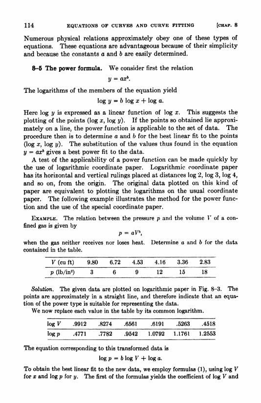
114 EQUATIONS OF CURVES AND CURVE FITTING [CHAP. 8
Numerous physical relations approximately obey one of these types of
equations. These equations are advantageous because of their simplicity
and because the constants a and b are easily determined.
8-5 The power formula. We consider first the relation
y = axb.
The logarithms of the members of the equation yield
log y = b log x + log a.
Here log y is expressed as a linear function of log x. This suggests the
plotting of the points (log #, log y). If the points so obtained lie approxi-
mately on a line, the power function is applicable to the set of data. The
procedure then is to determine a and b for the best linear fit to the points
(log x, log T/). The substitution of the values thus found in the equation
y = axbgives a best power fit to the data.
A test of the applicability of a power function can be made quickly bythe use of logarithmic coordinate paper. Logarithmic coordinate paper
has its horizontal and vertical rulings placed at distances log 2, log 3, log 4,
and so on, from the origin. The original data plotted on this kind of
paper are equivalent to plotting the logarithms on the usual coordinate
paper. The following example illustrates the method for the power func-
tion and the use of the special coordinate paper.
EXAMPLE. The relation between the pressure p and the volume V of a con-
fined gas is given by
p = aV\
when the gas neither receives nor loses heat. Determine a and b for the data
contained in the table.
T(cuft) 9.80 6.72 4.53 4.16 3.36 2.83
p (lb/in2) 3 6 9 12 15 18
Solution. The given data are plotted on logarithmic paper in Fig. 8-3. The
points are approximately in a straight line, and therefore indicate that an equa-
tion of the power type is suitable for representing the data.
We now replace each value in the table by its common logarithm.
logF .9912 .8274 .6561 .6191 .5263 .4518
logp .4771 .7782 .9542 1.0792 1.1761 1.2553
The equation corresponding to this transformed data is
log p b log V + log a.
To obtain the best linear fit to the new data, we employ formulas (1), using log Vfor x and log p for y. The first of the formulas yields the coefficient of log V and

8-5] THE POWER FORMULA 115
the second the constant term lop; a. We have the following sums:
2 log V = 4.0719, 2 (log I')5 = 2.9610,
2 log />= 5.7201, 2(log r)(log />)
= 3.5971.
Substituting these values and n =6, we get
6(3.5971)- 4.0719(5.7201)
"6(2.9619) -(4.0719)*
2.9620(5.7201) - 4.0719(3.5961)-- - -a = 84.6.
Making these substitutions for a and 6, we have
p = 84.6 V- 1 - 43
The graph of this equation and the points representing the original data are shown
in Fig. 8-4.
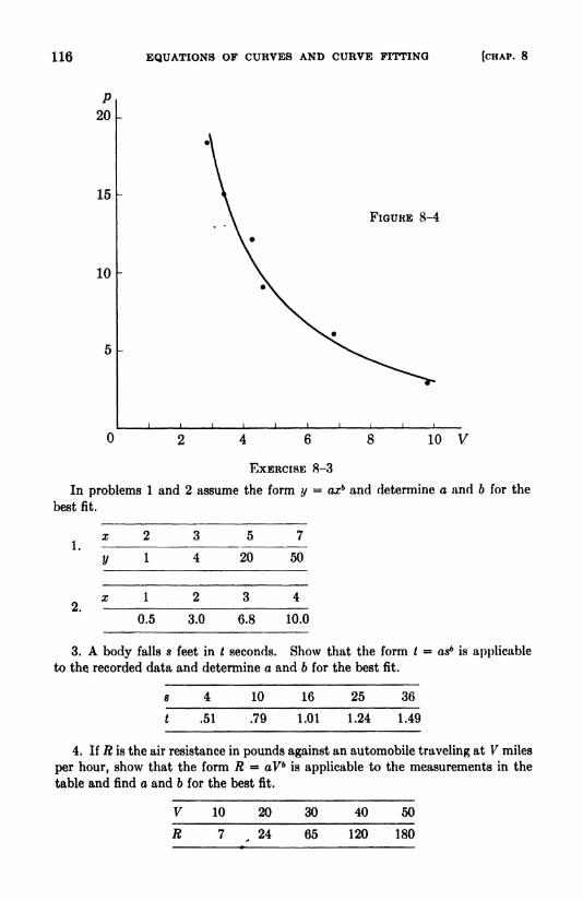
116 EQUATIONS OF CURVES AND CURVE FITTING [CHAP. 8
P20
15
10
FIGURE 8-4
8 10 V
EXERCISE 8-3
In problems 1 and 2 assume the form y = axb and determine a and b for the
best fit.
1.
2.
3. A body falls s feet in t seconds. Show that the form t asbis applicable
to the. recorded data and determine a and 6 for the best fit.
10 16 25 36
t .51 .79 1.01 1.24 1.49
4. If R is the air resistance in pounds against an automobile traveling at V miles
per hour, show that the form R = aVb is applicable to the measurements in the
table and find a and b for the best fit.
10 20 30 40 50
R 24 65 120 180
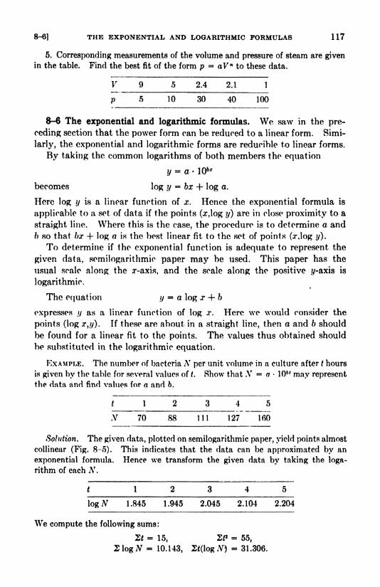
8-6] THE EXPONENTIAL AND LOGARITHMIC FORMULAS 117
5. Corresponding measurements of the volume and pressure of steam are givenin the table. Find the best fit of the form p = aV n to these data.
V 9 5 2.4 2.1 1
p 5 10 30 40 100
8-6 The exponential and logarithmic formulas. We saw in the pre-
ceding section that the power form can be reduced to a linear form. Simi-
larly, the exponential and logarithmic forms are reducible to linear forms.
By taking the common logarithms of both members the equation
y = a 106*
becomes log y bx + log a.
Here log y is a linear function of J. Hence the exponential formula is
applicable to a set of data if the points (x,log y) are in close proximity to a
straight line. Where this is the case, the procedure is to determine a and
b so that bx + log a is the best linear fit to the set of points (:r,log y).
To determine if the exponential function is adequate to represent the
given data, somilogarithmic paper may be used. This paper has the
usual scale along the x-axis, and the scale along the positive z/-axis is
logarithmic.
The equation y = a log x + b
expresses // as a linear function of log x. Here we would consider the
points (log x,y). If these are about in a straight line, then a and b should
be found for a linear fit to the points. The values thus obtained should
be substituted in the logarithmic equation.
EXAMPLE. The number of bacteria AT
per unit volume in a culture after t hours
is given by the table for several values of t. Show that A" = a 106/ may represent
the data and find values for a and 6.
t 1
.V 70 88 111 127 160
Solution. The given data, plotted on semilogarithmic paper, yield points almost
collinear (Fig. 8-5). This indicates that the data can be approximated by an
exponential formula. Hence we transform the given data by taking the loga-
rithm of each Ar.
t 1
log AT 1.845 1.945 2.045 2.104 2.204
We compute the following sums:
2t = 15, 2*2 = 55,
2 log N = 10.143, 2*(logW) = 31.306.

118 EQUATIONS OF CURVES AND CURVE FITTING [CHAP. 8
150
100
502 3
FIGURE 8-6
5 t
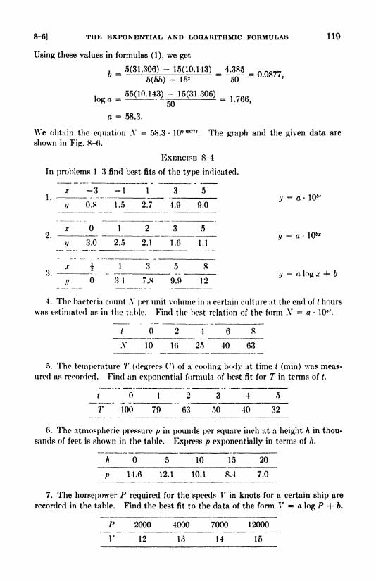
8~6] THE EXPONENTIAL AND LOGARITHMIC FORMULAS 119
Using these values in formulas (1), we get
5(31.306) - 15(10.143) 4.385nft?76 =
5(65)- 15*
="50"
='0877
'
. 55(10.143)-
15(31.306) , ^log a = ^
'--^^ L =
1.766,
a = 58.3.
We obtain the equation Ar = 58.3 1000877 '. The graph and the given data are
shown in Fig. 8-0.
EXERCISE 8-4
In problems 1 3 find best fits of the type indicated.
-3-1 1 3
0.8 1.5 2.7 4.9 9.0
2. y = a - 106*
y = a log x + b
4. The bacteria count .V per unit volume in a certain culture at the end of t hours
was estimated as in the table. Find the best relation of the form AT = a 10*'.
f 02468.V 10 16 25 40 63
5. The temperature T (degrees C) of a cooling body at time t (min) was meas-
ured as recorded. Find an exponential formula of best fit for T in terms of t.
t 012345T 100 79 63 50 40 32
6. The atmospheric pressure /) in pounds per square inch at a height h in thou-
sands of feet is shown in the table. Express p exponentially in terms of h.
h 5 10 15 20
~~P iTe 12! un &A 7.0
7. The horsepower P required for the speeds V in knots for a certain ship are
recorded in the table. Find the best fit to the data of the form V = a log P + b.
P 2000 4000 7000 12000
~V 12 13 14 15

CHAPTER 9
POLAR COORDINATES
9-1 Introduction. There are various types of coordinate systems. The
rectangular system with which we have been dealing is probably the most
important. In it a point is located by its distances from two perpendicularlines. We shall introduce in this chapter a coordinate system in which
the coordinates of a point in a plane are its distance from a fixed point andits direction from a fixed line. The coordinates given in this way are
called polar coordinates. The proper choice of a coordinate system de-
pends on the nature of the problem at hand. For some problems either
the rectangular or the polar system may be satisfactory; usually, however,one of the two is preferable. And in some situations it is advantageousto use both systems, shifting from one to the other.
9-2 The polar coordinate system. The reference frame in the polarcoordinate system is a half-line drawn from some point in the plane. In
Fig. 9-1 a half-line is represented by OA. The point is called the originor pole and OA is the polar axis. The position of any point P in the planeis definitely determined by the distance OP and the angle AOP. Thesegment OP, denoted by p, is referred to as the radius vector; the angleAOP, denoted by 0, is called the vectorial angle. The coordinates of P are
then written as (p,0).
It is customary to regard polar coordinates as signed quantities. Thevectorial angle, as in trigonometry, is defined as positive or negative ac-
cording as it is measured counterclockwise or clockwise from the polaraxis. The p-coordinate is defined as positive if measured from the pole
along the terminal side 'of 6 and negative if measured along the terminal
side extended through the pole.
A given pair of polar coordinates definitely locates a point. For
example, the coordinates (2,30) determine one particular point. To plotthe point, we first draw the terminal side of a 30 angle measured counter-
clockwise from OA (Fig. 9-2) and then lay off two units along the terminal
side. While this pair of coordinates defines a particular point, there are
other coordinate values which define this same point. This is evident,since the vectorial angle may have 360 added or subtracted repeatedlywithout changing the point represented. Additional coordinates of the
point may be had also by using a negative value for the distance coordi-
nate. Restricting the vectorial angles to values numerically less than120
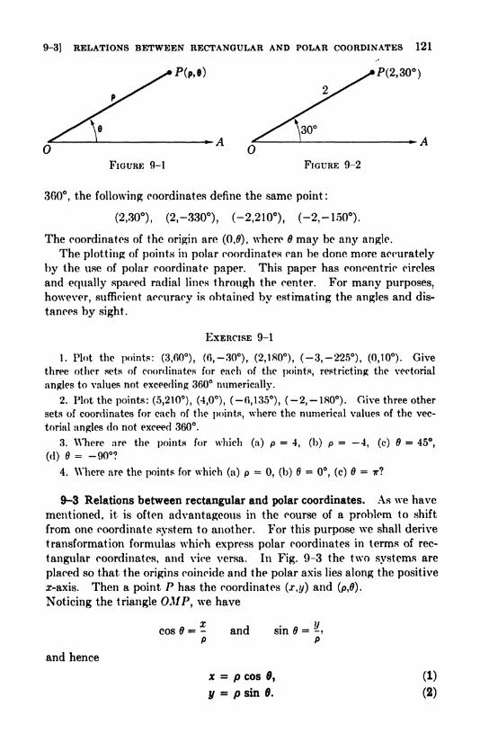
9-3] RELATIONS BETWEEN RECTANGULAR AND POLAR COORDINATES 121
'P(M)
V A
FIGURE 9-1 FIGURE 9-2
300, the following coordinates define the same point :
(2,30), (2,-330), (-2,210), (-2,-150).
The coordinates of the origin are (0,0), where 6 may be any angle.
The plotting of points in polar coordinates can be done more accurately
by the use of polar coordinate paper. This paper has concentric circles
and equally spaced radial lines through the center. For many purposes,
however, sufficient accuracy is obtained by estimating the angles and dis-
tances by sight.
EXERCISE 9-1
1. Plot the points: (3,60), (6, -30), (2,180), (-3, -225), (0,10). Give
three other sets of coordinates for each of the points, restricting the vectoriai
angles to values not exceeding 360 numerically.
2. Plot the points: (5,210), (4,0), (-0,135), (-2, -180). Give three other
sets of coordinates for each of the points, where the numerical values of the vec-
toriai angles do not exceed 360.
3. Where are the points for which (a) p =4, (b) p =
4, (c) 6 = 45,
(<1)= -90?
4. Where are the points for which (a) p =0, (b) 8 = 0, (c) 6 = TT?
9-3 Relations between rectangular and polar coordinates. As we have
mentioned, it is often advantageous in the course of a problem to shift
from one coordinate system to another. For this purpose we shall derive
transformation formulas which express polar coordinates in terms of rec-
tangular coordinates, and vice versa. In Fig. 9-3 the two systems are
placed so that the origins coincide and the polar axis lies along the positive
x-axis. Then a point P has the coordinates (x,y) and (p,0).
Noticing the triangle OAfP, we have
x ?/
cos 6 = - and sin B = ->
p P
and hence
x = p cos 0, (1)
y = p sin 0. (2)

122
y
POLAR COORDINATES [CHAP. 9
(p,e)
M -X
FIGURE 9-3
To obtain p and 6 in terms of x and y, we write
p2 = x2 + y* and
Whence, solving for p and 8,
tan 6 = .
x
= arc tan -
(3)
(4)
These four formulas enable us to transform the coordinates of a point,
and therefore the equation of a locus, from one system to the other. The^-coordinate as given by formula (4) is not single-valued. Hence it is
necessary to select a proper value for 6 when applying the formula to find
this coordinate of a point. This is illustrated in Example 2.
EXAMPLE 1. Find the rectangular coordinates of the point defined by the
polar coordinates (6,120). (See Fig. 9-4.)
Solution. Using the formulas (1) and (2), we have
x = p cos0 = 6 cos 120 = -3,
y = p sin 6 = 6 sin 120 = 3\/3.
The required coordinates are ( 3,3Vs).
EXAMPLE 2. Express the rectangular coordinates (2, 2) in terms of polar
coordinates.
Solution. Here the formulae (3) and (4) give
p = Vx2 + y*= 2\/2 and 8 = arc tan - = arc tan 1.
x
Since the point is in the third quadrant, we select 6 = 225. Hence the pair of
coordinates (2V2,225) is a polar representation of the given point.
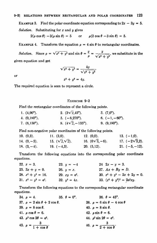
9-3] RELATIONS BETWEEN RECTANGULAR AND POLAR COORDINATES 123
EXAMPLE 3. Find the polar coordinate equation corresponding to 2x 3y = 5.
Solution. Substituting for x and y gives
2(p cos 6) -3(p sin 6)= 5 or p(2 cos 6 -3 sin 6)
= 5.
EXAMPLE 4. Transform the equation p = 4 sin 6 to rectangular coordinates.
Solution. Since p = Vz2 + ?/2 and sin 6 = - = ====., we substitute in the
given equation and get
V*2 + v*v/z2 + y
2
or
*2 + */2 = 40.
The required equation is seen to represent a circle.
EXERCISE 9-2
Find the rectangular coordinates of the following points.
1. (4,90). 2. (3x^2,45). 3. (7,0).
4. (0,1 SO ). 5. (-8,270). 6. (-1,-60).
7. (6,150). 8. (4V2,-135). 9. (9,180).
Find non-negative polar coordinates of the following points.
10. (0,3). 11. (3,0). 12. (0,0). 13. (-1,0).
14. (0,-5). 15. (\/2,\/2). 16. (ev^-e). 17. (-2\/3,2).
18. (3,-4). 19. (-4,3). 20. (5,12). 21. (-5,-12).
Transform the following equations into the corresponding polar coordinate
equations.
22. x = 3. 23. y = -4 24 2x - y = 3.
25. 3x + y = 0. 26. y = x. 27. Ax + By = D.
28. a-2 + if
= 16. 29. j?/= a2
. 30. x2 + i/
2 - 2x + 2y = 0.
31. J2 -y2 = a2
. 32. .v
2 = 4j. 33. Or2 + ?/
2)2
Transform the following equations to the corresponding rectangular coordinate
equations.
34. p = 4. 35. 6 = 0. 36. 6 = 45.
37. p 2 sin + 2 cos 0. 38. p = 6 sin 4 cos
39. p = 8 cos 6. 40. p = 8 sin 0.
41. p cos = 6. 42. p sin 6 = 6.
43. p2 cos 26 = a2
. 44. p2 sin 26 = a2
.
3
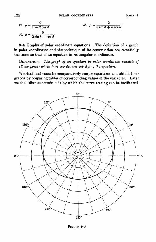
124
47. p-
49. p =
1 - 2 cos 6
5
2 sin cos 6
POLAR COORDINATES
48. p =
[CHAP. 9
3 sin + 4 cos 6
9-4 Graphs of polar coordinate equations. The definition of a graphin polar coordinates and the technique of its construction are essentially
the same as that of an equation in rectangular coordinates.
DEFINITION. The graph of an equation in polar coordinates consists of
all the points which have coordinates satisfying the equation.
We shall first consider comparatively simple equations and obtain their
graphs by preparing tables of corresponding values of the variables. Later
we shall discuss certain aids by which the curve tracing can be facilitated.
120' 60
ISO / 30
210'

9-4] GRAPHS OF POLAR COORDINATE EQUATIONS 125
EXAMPLE 1. Draw the graph of p 3 + sin 0.
Solution. We assign certain values to in the interval to 360 and prepare
the following table.
By plotting these points and drawing a curve through them the graph of Fig, 9-5
is obtained.
FIGURE 9-6
EXAMPLE 2. Draw the graph of p = 4 cos 6.
Solution. We first prepare a table of corresponding values of p and 6.
B 30 45 60 75 90 120 135 150 180
~~p 4 3J5 2^8 2X) To" -2.0 -2.8 -3.5 -4
This table yields the graph in Fig. 9-6. We did not extend the table to include
values of 6 in the interval 180 to 360, since values of in this range would merely
repeat the graph already obtained. For example, the point (3.5,210) is on the
graph, but this point is also defined by the coordinates (3.5,30).
The graph appears to be a circle. This surmise is verified by transforming the
equation to rectangular coordinates. The transformed equation is (j 2)2-f if
= 4.
EXERCISE 9-3
Draw the graphs of the following equations. In the equations involving trigo-
nometric functions, points plotted at 30 intervals will suffice, with a few exceptions.
1. p = 5. 2. p = -5. 3. 6 = 120.
4. B - 180. 5. p = 1 - cos 0. 6. p = 1 - sin 6.

126 POLAR COORDINATES [CHAP. 9
7. p = 2 + cos 0.
10. p = 2a cos 0.
13 p =sin0'
19. p = 10 sin2 0.
22. p = 4 sin - 4 cos 6. 23. p = 8 sin 6 + 6 cos 6.
9-5 Equations of lines and conies in polar coordinate forms. The
equations of lines and conies can be obtained in polar coordinates bytransforming the rectangular coordinate equations of these loci. The
equations can also be derived directly. We shall derive the polar coor-
dinate equation of a line in general position and the equations of the conic
sections in special positions.
In Fig. 9-7 the segment OR is drawn perpendicular to the line L. Wedenote the length of this segment by p and the angle which it makes with
the polar axis by w. The coordinates of a variable point on the line are
(p,0). From the right triangle ORP, we have
- = cos (6-
w)p
or
p cos (9-
o>)= p. (6)
This equation holds for all points of the line. If P is chosen below OA,then the angle ROP is equal to (w + 2w - 0). Although this angle is not
equal to (0 w), we do have cos (co + 2w 0)= cos (w 0)
= cos (0 w).
In a similar way, the equation could be derived for the line L in any other
position and not passing through the origin.
VFIGURE 9-7
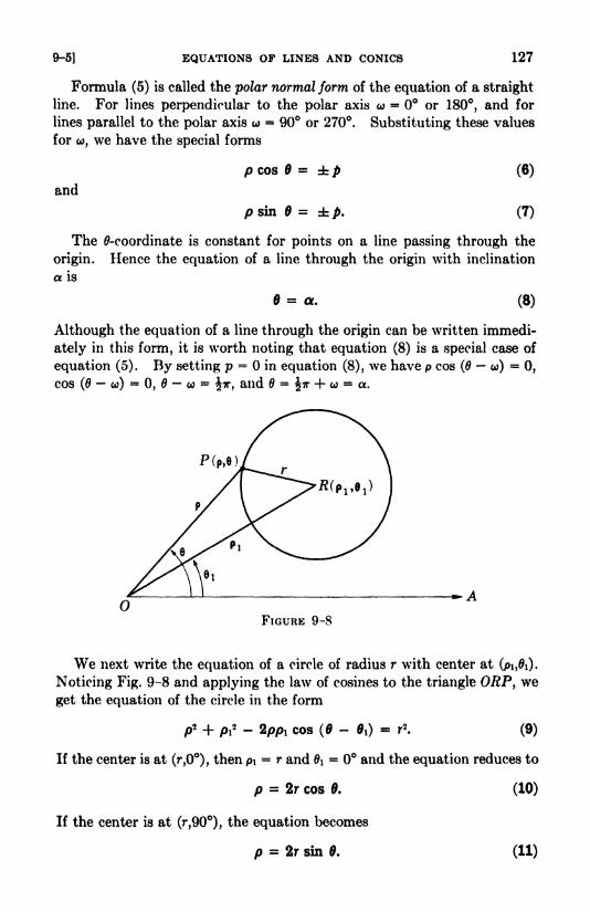
9-5] EQUATIONS OF LINES AND CONICS 127
Formula (5) is called the polar normal form of the equation of a straight
line. For lines perpendicular to the polar axis co = or 180, and for
lines parallel to the polar axis = 90 or 270. Substituting these values
for co, we have the special forms
P COS s= p (6)
and
psin = p. (7)
The ^-coordinate is constant for points on a line passing through the
origin. Hence the equation of a line through the origin with inclination
a is
= a. (8)
Although the equation of a line through the origin can be written immedi-
ately in this form, it is worth noting that equation (8) is a special case of
equation (5). By setting p = in equation (8), we have p cos (6 co)=
0,
cos (0 co)=
0, 6 co = i?r, and =JTT + co = a.
P(p,8)
FIGURE 9-8
We next write the equation of a circle of radius r with center at (pi,0i).
Noticing Fig. 9-8 and applying the law of cosines to the triangle ORP, we
get the equation of the circle in the form
p2 + p!
2 - 2pp! cos ($-
tfi)= r2 . (9)
If the center is at (r,0), then pi= r and 0i = and the equation reduces to
p = 2r cos fl. (10)
If the center is at (r,90), the equation becomes
p = 2r sin 9. (11)

128 POLAR COORDINATES [CHAP. 9
E
D
P(p,e)
P
FIGURE 9-9
R
We use the focus-directrix property of conies (Exercise 8-1, problem 15)
to derive their equations in polar coordinates. The equations can be ob-
tained in simple forms if the focus and origin coincide and the directrix
is parallel or perpendicular to the polar axis. In Fig. 9-9 the directrix DEis perpendicular to the polar axis and to the left of O. If we indicate the
eccentricity by e, and the length of DO by p, we have for any point P(p,0)
of the conic
OPEP e.
But the numerator OP =p, and the denominator EP = DR = DO + OR
= p + p cos 6. Hence p/(p + p cos 6)=
e, and solving for p, we get
epP =
1 - e cos (12)
When the focus is at the pole and the directrix is p units to the right of
the pole, the equation is
.
1 -f e cos 9(13)
If the focus is at the pole and the directrix is parallel to the polar axis,
the equation is
or
P ~1 + sin B
__,1 e sin 9
P =
(14)
(15)
depending on whether the directrix is p units above or below the pole.
An equation in any of the forms (12) -(15) represents a parabola if
e = 1, an ellipse if e is between and 1, and a hyperbola if e is greaterthan 1. The graph in any case can be sketched immediately. Havingobserved the type of conic from the value of e, the next step is to find the
points where the curve cuts the polar axis, the extension of the axis through
0, and the line through the pole perpendicular to the polar axis. These

9-5] EQUATIONS OF LINES AND CONICS 129
are called the intercept points, and may be obtained by using the values 0,90, 180, and 270 for 6. Only three of these values can be used for a
parabola, since one of them would make a denominator zero. The inter-
cept points are sufficient for a rough graph. For increased accuracy a
few additional points should be plotted.
(3,180;
FIGURE 9-10
EXAMPLE. Sketch the graph of p = 15/(3 2 cos 6).
Solution. The equation takes the form (12) when the numerator and denomi-
nator of the right member are divided by 3. This gives
P =1-
(2/3) cos 6
In this form we observe that e 2/3, and hence the graph is an ellipse. Substi-
tuting 0, 90, 180, and 270 in succession for in the original equation, the inter-
cept points are found to be
(15,0), (5,90), (3,180), and (5,270).
These points are plotted in Fig. 9-10. The points (15,0) and (3, 180) 'are vertices
and the other intercept points are the ends of a latus rectum. The center, mid-
way between the vertices, is at (6,0). The length of the major axis 2a =18,
and a = 9. The distance between the center and the focus at is c = 6. Hence
52 = fl2_ C2 = 81 _ 36 =
45> an(j b = 3v/5.
EXERCISE 9-4
1. By use of a figure find the equation of the line perpendicular to the polar
axis and (a) 3 units to the right of the pole, (b) 3 units to the left of the pole.
Compare your results with formula (6).
130 POLAR COORDINATES [CHAP. 9
2. By use of a figure find the equation of the line parallel to the polar axis
and (a) 3 units below the axis, (b) 3 unite above the axis. Check your results
with formula (7).
3. Show that formula (5) can be reduced to the form
= Cp Acosd + BsmB'
Plot two points and draw the line represented by each equation 4-6.
6. p =
+ 2 sin' H
2 cos B - sin 6
-32 cos + 5 sin
Give the coordinates of the center and the radius of each circle defined by
equations 7-10.
7. p = 8 cos 0. 8. p = 6 sin 0.
9 p = -10 sin 0. 10. p= -4cos0.
1 1 . Use formula (9) and write the equation of the circle of radius 2 and (a) with
center at (4,0), (b) with center at (4,90), (c) with center at (2,0).
Sketch the conies defined by equations 12-23.
13 -
+sin0
1,19 1C 10
14 ' P - o.o a' 15 '
2cos0 H3 -3sin0
12 _ 12
2 - cos0 ^2 + sin0
0121. p =
5 -4sin010
wt "1 -2cos0
~' "2 + 3cos0
oo ft = 1590 A = 18
P3 + 5sin0
' p 3-4sin0'
9-6 Aids in graphing polar coordinate equations. We have seen that
an examination of an equation in rectangular coordinates may reveal
short-cuts to the construction of its graph. In the same way, certain
features of a graph in polar coordinates are often discovered by an analysis
of its equation. It is better, for economy of time, to wrest useful informa-
tion from an equation and thus keep at a minimum the tedious point-by-
point plotting in sketching a graph. We shall discuss and illustrate cer-
tain simple devices in polar curve tracing.
Variation of p with 0. Many equations are sufficiently simple so that
the way in which p varies as increases is evident. Usually a range of
0-values from to 360\yields the complete graph. However, we shall
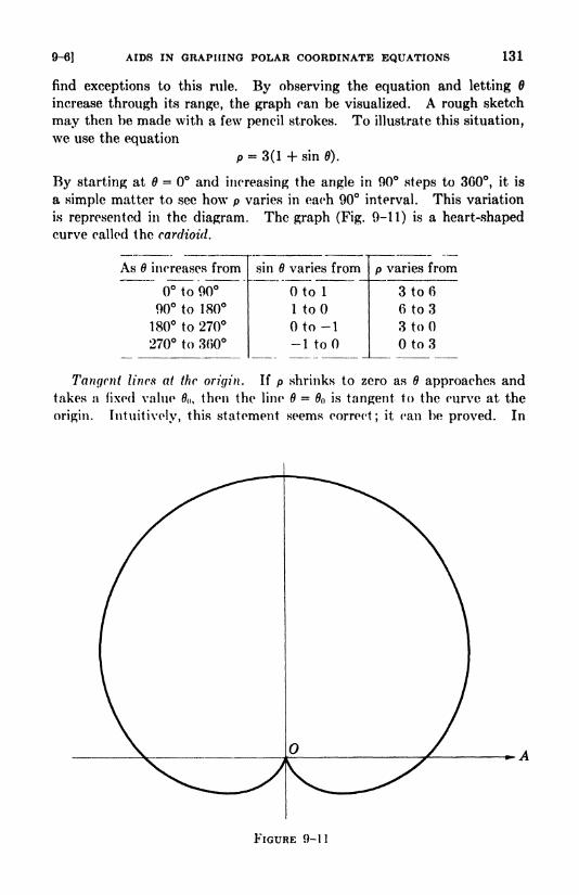
9-6] AIDS IN GRAPHING POLAR COORDINATE EQUATIONS 131
find exceptions to this rule. By observing the equation and letting
increase through its range, the graph ran be visualized. A rough sketch
may then be made with a few pencil strokes. To illustrate this situation,
we use the equation
p = 3(1 + sin 0).
By starting at 6 = and increasing the angle in 90 steps to 360, it is
a simple matter to see how p varies in each 90 interval. This variation
is represented in the diagram. The graph (Fig. 9-11) is a heart-shapedcurve called the cardioid.
Tangent lines at the origin. If p shrinks to zero as 6 approaches and
takes a fixed value 0<, then the lino 6 n is tangent to the curve at the
origin. Intuitively, this statement seems correct; it can be proved. In
FIGURE 9-11
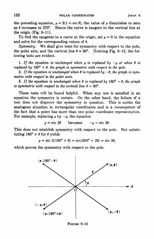
132 POLAR COORDINATES [CHAP. 9
the preceding equation, p = 3(1 + sin 0), the value of p diminishes to zero
as increases to 270. Hence the curve is tangent to the vertical line at
the origin (Fig. 9-11).
To find the tangents to a curve at the origin, set p = in the equationand solve for the corresponding values of 6.
Symmetry. We shall give tests for symmetry with respect to the pole,
the polar axis, and the vertical line 8 = 90. Noticing Fig. 9-12, the fol-
lowing tests are evident.
1. // the equation is unchanged when p is replaced by p or when 6 is
replaced by 180 4- 6, the graph is symmetric with respect to the pole.
2. // the equation is unchanged when is replaced by 0, the graph is sym-metric with respect to the polar axis.
3. // the equation is unchanged when 6 is replaced by 180 0, the graphis symmetric with respect to the vertical line 6 = 90.
These tests will be found helpful. When any one is satisfied in an
equation the symmetry is certain. On the other hand, the failure of a
test does not disprove the symmetry in question. This is unlike the
analogous situation in rectangular coordinates and is a consequence of
the fact that a point has more than one polar coordinate representation.
For example, replacing p by p, the equation
p = sin 26 becomes p = sin 26.
This does not establish symmetry with respect to the pole. But substi-
tuting 180 + $ for 6 yields
p = sin 2(180 + 0)= sin(360 + 26)
= sin 26,
which proves the symmetry with respect to the pole.
(P,180-6)(P,O)
(-P,
(p,i80+e)
FIGURE 9-12

9-7] SPECIAL TYPES OP EQUATIONS 133
Continuing with the equation
p = sin 20,
we see that it does not satisfy tests 2 and 3. But it is sufficient to obtain
the graph for from to 180, and then to complete the drawing by the
known symmetry with respect to the pole. Since we have a trigonometricfunction of 20, it is convenient to consider the variation of p as 6 increases
in steps of 45. The diagram indicates this variation. From it we see
FIGURE 9-13
the values of corresponding to the zero value of p, and therefore conclude
that the graph is tangent to the polar axis and the vertical line at the
origin. Having completed the graph (Fig. 9-13), it is seen that it has
all three types of symmetry. Because of its shape, the graph is called a
four-leaved rose. The barbs and numbers indicate how a point would
move in tracing the curve as increases from to 300.
Excluded values. Frequently equations are met in which certain values
of the variables are excluded. For example, p2 = a2 sin places restrictions
on both p and 0. The values of p are in the range a to a, and cannot
have a value between 180 and 300, since p is imaginary for these values.
The curve extends into the third and fourth quadrants, however, since
the graph is symmetric with respect to the origin.
9-7 Special types of equations. There are several types of polar co-
ordinate equations whose graphs have been given special names. Weconsider a few of these equations.
The graphs of equations of the forms
p = a sin n0 and p = a cos n0,
where n is a positive integer, are called rose curves. The graph of a rose
curve consists of equally spaced closed loops extending from the origin.
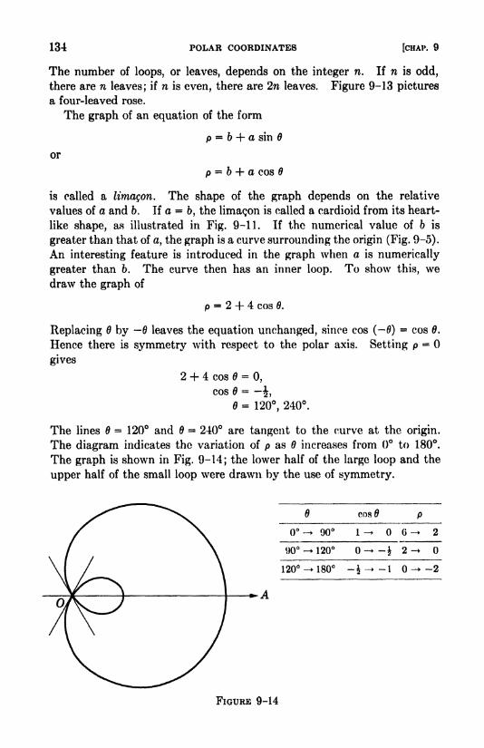
134 POLAR COORDINATES [CHAP. 9
The number of loops, or leaves, depends on the integer n. If n is odd,
there are n leaves; if n is even, there are 2n leaves. Figure 9-13 pictures
a four-leaved rose.
The graph of an equation of the form
or
p = 6 + a sin
p = b + a cos
is called a limagon. The shape of the graph depends on the relative
values of a and b. If a = 6, the limagon is called a cardioid from its heart-
like shape, as illustrated in Fig. 9-11. If the numerical value of b is
greater than that of a, the graph is a curve surrounding the origin (Fig. 9-5).
An interesting feature is introduced in the graph when a is numerically
greater than b. The curve then has an inner loop. To show this, we
draw the graph of
p = 2 + 4 cos e.
Replacing by leaves the equation unchanged, since cos (0) = cos 0.
Hence there is symmetry with respect to the polar axis. Setting p =
gives
2 + 4 cos =0,
cos =J,
= 120, 240.
The lines = 120 and = 240 are tangent to the curve at the origin.
The diagram indicates the variation of p as increases from to 180.
The graph is shown in Fig. 9-14; the lower half of the large loop and the
upper half of the small loop were drawn by the use of symmetry.
cos0
90 6
90 -* 120 -i 2
120 180 - -l 0-+-2
FIGURE 9-14
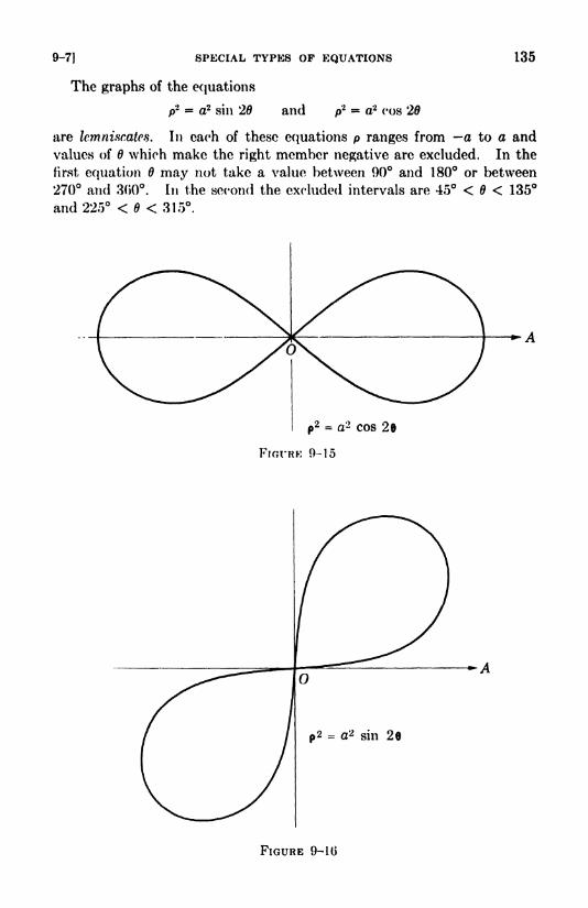
9-7] SPECIAL TYPES OP EQUATIONS
The graphs of the equations
p2 = a2 sin 28
135
and a2 cos 20
are Icmniscates. In each of these equations p ranges from a to a and
values of 6 which make the right member negative are excluded. In the
first equation may not take a value between 90 and 180 or between
270 and 300. In the second the excluded intervals are 45 < 6 < 135
and 225 < 9 < 315.
p2 = a2 cos 28
FIGURK 9-15
FIGURE 9-10
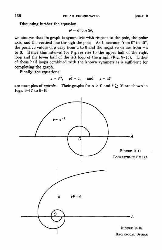
136 POLAR COORDINATES [CHAP. 9
Discussing further the equation
p2 = a2 cos 20,
we observe that its graph is symmetric with respect to the pole, the polar
axis, and the vertical line through the pole. As increases from to 45,the positive values of p vary from a to and the negative values from a
to 0. Hence this interval for gives rise to the upper half of the right
loop and the lower half of the left loop of the graph (Fig. 9-15). Either
of these half loops combined with the known symmetries is sufficient for
completing the graph.
Finally, the equations
p = e *, p6 = a, and p = aO,
are examples of spirals.
Figs. 9-17 to 9-19.
Their graphs for a > and > are shown in
FIGURE 9-17
LOGARITHMIC SPIRAL
FIGURE 9-18
RECIPROCAL SPIRAL
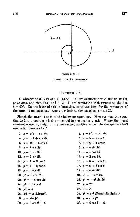
9-7] SPECIAL TYPES OF EQUATIONS 137
FIGURE 9-19
SPIRAL OF ARCHIMEDES
EXERCISE 9-5
1. Observe that (p,0) and ( p,180 6) are symmetric with respect to the
polar axis, and that (p,0) and ( p, 0) are symmetric with respect to the line
= 90. On the basis of this information, state two tests for the symmetry of
the graph of an equation. Apply the tests to the equation p= sin 26.
Sketch the graph of each of the following equations. First examine the equa-
tion to find properties which are helpful in tracing the graph. Where the literal
constant a occurs, assign to it a convenient positive value. In the spirals 25-29
use radian measure for 0.
2. p = 4(1-
cos0).
4. p = a(l -f cos0).
6. p = 10 - 5 cos 0.
8. p = 8 cos 20.
10. p = 6 sin 30.
12. p = 2 sin 50.
14. p = 4 8 cos 0.
16. p = 4 + 8 cos 0.
18. p = a cos 40.
20. p2 = 9 cos 20.
22. p2 = -a2 cos 20.
24. p2 = a2 cos 0.
26. p0 = 4.
28. p2 = a (Lituus).
30. p = sin 0.
32. p - 3 sec -f 4.
3. p = 6(1- sin 0).
5. p = 5 - 2 sin 0.
7. p = 8 -f 4 cos 0.
9. p = a sin 20.
11. p = 4 cos 30.
13. p = 2 cos 50.
15. p = 6 3sin0.
17. p = 6 4- 3 sin 0.
19. p = a sin 40.
21. p2 = 16 sin 20.
23. p2 = -a2 sin 20.
25. p = 20.
27. p = e*.
29. p2 - a2
(Parabolic Spiral).
31. p = cos0.
33. p = 6 sec - 6,
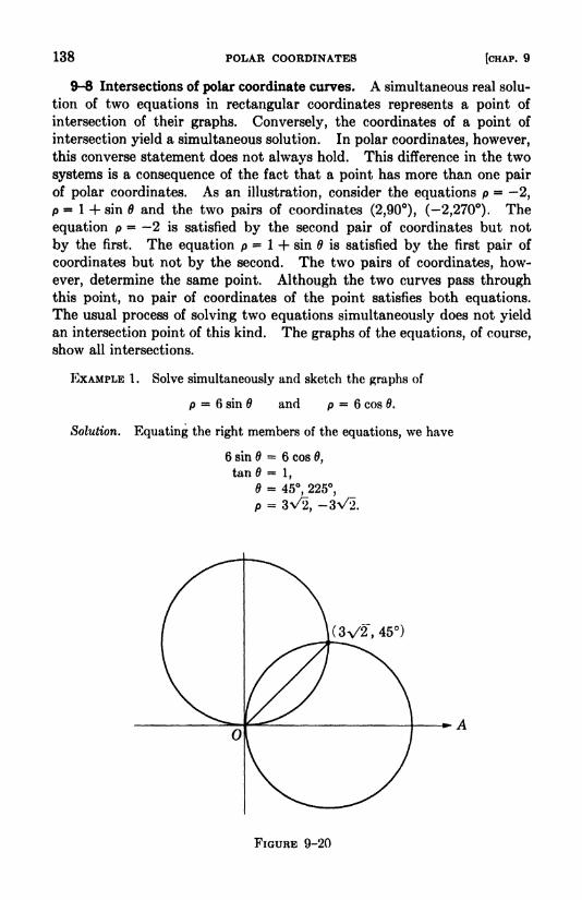
138 POLAR COORDINATES [CHAP. 9
9-8 Intersections of polar coordinate curves. A simultaneous real solu-
tion of two equations in rectangular coordinates represents a point of
intersection of their graphs. Conversely, the coordinates of a point of
intersection yield a simultaneous solution. In polar coordinates, however,this converse statement does not always hold. This difference in the two
systems is a consequence of the fact that a point has more than one pair
of polar coordinates. As an illustration, consider the equations p = -2,
p - 1 + sin 6 and the two pairs of coordinates (2,90), (-2,270). The
equation p = 2 is satisfied by the second pair of coordinates but not
by the first. The equation p = 1 + sin is satisfied by the first pair of
coordinates but not by the second. The two pairs of coordinates, how-
ever, determine the same point. Although the two curves pass throughthis point, no pair of coordinates of the point satisfies both equations.
The usual process of solving two equations simultaneously does not yield
an intersection point of this kind. The graphs of the equations, of course,
show all intersections.
EXAMPLE 1 . Solve simultaneously and sketch the graphs of
p = 6 sin 6 and p = 6 cos 0.
Solution. Equating the right members of the equations, we have
6 sin = 6 cos 0,
tan0 =1,
6 =45,_225,
p =
(3v/2, 45)
FIGURE 9-20
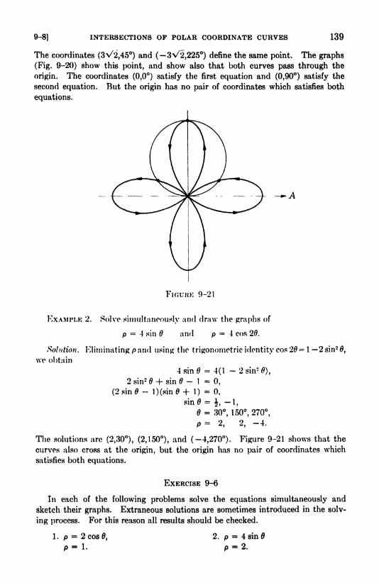
9-8] INTERSECTIONS OF POLAR COORDINATE CURVES 139
The coordinates (3V2,45) and (-3V2,225) define the same point. The graphs
(Fig. 9-20) show this point, and show also that both curves pass through the
origin. The coordinates (0,0) satisfy the first equation and (0,90) satisfy the
second equation. But the origin has no pair of coordinates which satisfies both
equations.
FIGURE 0-21
EXAMPLE 2. Solve simultaneously and draw the graphs of
p = 4 sin 6 and p = 4 cos 20.
Solution. Eliminating p and using the trigonometric identity cos2012 sin20,
we obtain
4sin0 = 4(1- 2sin2
0),
2 sin24- sin -
1 =0,
(2 smB -I)(sin0 + 1)
= 0,
sin0 =i, -1,
= 30, 150, 270,
P= 2, 2, -4.
The solutions are (2,30), (2,150), and (-4,270). Figure 9-21 shows that the
curves also cross at the origin, but the origin has no pair of coordinates which
satisfies both equations.
EXERCISE 9-6
In each of the following problems solve the equations simultaneously and
sketch their graphs. Extraneous solutions are sometimes introduced in the solv-
ing process. For this reason all results should be checked.
1. p = 2cos0,
P- 1-
2. p = 4 sin
p-2.
140 POLAR COORDINATES [CHAP. 9
3. p = 6 cos 0,
p cos 6 = 3.
5. p = a(l + cos 0),
p o(l cos0).
7. p2 4 cos 0,
9 ' p " T3p cos = 2.
11. p = 2sin0 + 1,
p = cos 0.
13. p = 2 sin 0,
= 60.
15. p = 2 sin J0,
p=l.17. p = 4 + cos 0,
pcos0 = 3.
19. p = 2cos0 + 1,
pcos = 1.
4. p = a(l + sin 0),
p = 2a sin 0,
6. pcos0 =1,
p = 2.
8. p 1 + sin 0,
p - 1 + cos 0.
g10 - p = 4-3COS0'
p = 3 cos 0.
12. p2 = a2
sjn 20,
p - aV2 cos 0.
14. p = sin2 0,
p - cos20.
16. p = 1 - sin 0,
p = cos 20.
18. p = 4 - sin 0,
p sin = 3.
220. p
sin + cos 0*
2:
1 - cos0'
CHAPTER 10
PARAMETRIC EQUATIONS
10-1 Introduction. Relations between x and y up to this point have
been expressed by equations involving these variables. Another way of
defining a relation between x and y is through the use of two equationsin which each variable is expressed separately in terms of a third variable.
The third variable is called a parameter and the equations are called
parametric equations. Equations of this kind are of considerable im-
portance; the mathematical treatment of many problems is facilitated bytheir use. The equations
x = 2t and y = t 4,
for example, are parametric equations and t is the parameter. The equa-tions define a locus. If a value is assigned to t, corresponding values are
determined for x and ?/, which are the coordinates of a point of the locus.
The complete locus consists of the points determined in this way as t
varies through all its values. The relation between x and y is expressed
directly by eliminating t between the two equations. Thus solving either
of these equations for t and substituting in the other, we get
x - 2y = 8.
Often the parameter can be eliminated, as we have here done, to ob-
tain a direct relation. Sometimes, however, this process is not easy or
possible because the parameter is involved in a complicated way. The
equations
x = t* + log t and y = ^ 4- tan t
illustrate this statement.
It is sometimes helpful in the course of a problem to change an equation
in x and y to parametric form. Consider, for example, the parabola
defined byx2 + 2x + y - 4.
If we substitute 2t for x and solve the resulting equation for y, we get
y = 4 4J 4*2. Hence the parametric equations
x = 2t and y = 4 - 4* - 4?
represent the parabola. It is evident that other representations could be
obtained, since x may be equated to any function of t. This procedure is
141

142 PARAMETRIC EQUATIONS [CHAP. 10
inconvenient or perhaps impossible in equations which contain both
variables in an involved way.The parameter as here used plays a different role from the parameter
which we discussed in Section 3-5. Here the parameter is a variable, and
a curve is determined by letting the parameter vary through its range. In
contrast, the parameter in a linear equation in x and y gives rise to a family
of curves (lines). A line is determined by each value assigned to the
parameter.
10-2 Parametric equations of the circle and ellipse. To find a para-
metric representation of the circle of radius a and center at the origin, weselect for the parameter the angle 8 indicated in Fig. 10-1. We have at
once
x - a cos 6 and y = a sin 6.
If we let increase from to 360, the point (x,y), defined by these equa-
tions, starts at (a,0) and moves counterclockwise around the circle. Byletting change directly with the time / so that =
kt, the equations become
x = a cos kt and y = a sin kt.
TheThese equations give the location of the moving point at any time.
speed of the point is constant.
The equations x = a cos 6 and y = b sin 6 represent an ellipse. This
statement can be verified by eliminating the parameter 0. Writing the
equations as
- = cos 6a
and = sin 6,
FIGURE 10-1

10-3] THE GRAPH OF PARAMETRIC EQUATIONS 143
squaring both members of each equation, and adding, we get
From this result we see that the parametric equations represent an ellipse,
and we are able to interpret the quantities a and b. The geometric
significance of 6 can be seen in Fig. 10-2. The concentric circles are of
radii a and b. The terminal side of cuts the circles at A and B. Theintersection of the vertical line through A and the horizontal line throughB gives a point of the ellipse. For this point P, we have
x = OM = OA cos B = a cos 6,
y = MP = NB = OB sin 6 = b sin 0.
Hence as 6 varies, P moves along an ellipse. The ellipse is traced byletting 6 vary through 360. If starts at and increases to 360, the
point P starts at (a,0) and traces the ellipse in a counterclockwise direction.
FIGURE 10-2
10-3 The graph of parametric equations. To obtain the graph of two
parametric equations, we first assign to the parameter a set of values and
compute the corresponding values of x and y. We then use the plotted
points (x,y) for drawing the graph. An alternate procedure is to eliminate

144 PARAMETRIC EQUATIONS [CHAP. 10
the parameter and construct the graph of the resulting equation. In
some cases, however, the graph of the parametric equations is only a part
of the graph of the rectangular equation. Example 2 illustrates this case.
EXAMPLE 1. Sketch the graph of
x = 5t - P and y - 4* - P.
Solution. The table is the result of assigning to t the indicated values and
finding the corresponding values of x and y. The graph (Fig. 10-3) is the curve
drawn through the points (x,y) as determined by the table.
To eliminate the parameter between the preceding equations we subtract the
second equation from the first, which gives
x y =* t.
Then substituting x y for t in either of the given equations and simplifying, weobtain
x* 2xy + y*- 4x + 5y = 0.
By the test of Section 5-13 the graph is a parabola. The graph is probably more
easily obtained from the parametric equations than from the rectangular equation.
FIGURE 10-3
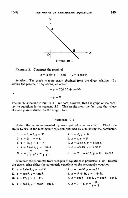
10-3] THE GRAPH OP PARAMETRIC EQUATIONS
Y
145
\
O \FIGURE 10-4
EXAMPLE 2. Construct the graph of
x = 2 sin 2 6 and y = 2 cos2 6.
Solution. The graph is more easily obtained from the direct relation. Byadding the parametric equations, we obtain
or
x + y = 2(sin2 6 + cos2
0)
r + y = 2.
The graph is the line in Fig. 10-4. We note, however, that the graph of the para-
metric equations is the segment AB. This results from the fact that the values
of x and y are restricted to the range to 2.
EXERCISE 10-1
Sketch the curve represented by each pair of equations 1-10. Check the
graph by use of the rectangular equation obtained by eliminating the parameter.
1. x = 2 -/,?/ = St.
3. x = er 1
, y = *.
5. x =3<, /y=l~ /
2.
7. x = 4 cos 0, y = 3 sin 0.
o 2 _ 2*J. X ^ ; T; W r
; ^'
2. a: = f2
, */= 4f
4. x =*, ?/
= e3
.
6. x = 5 sin 0, y
8. x = cos 20, y
5 cos 8.
2 sin 0.
10. x = 2 + 5 sin 0, y = 2 - 3 cos 0.
Eliminate the parameter from each pair of equations in problems 1 1-20. Sketch
the curve, using either the parametric equations or the rectangular equation.
11. x = 2 sin 0, y = cos2 0. 12. x = tan20, ^ = sec2
0.
13. x = sec 0,= tan 0. 14. x = J
2 + 4*, y = J2 + 3*.
15. x = r 1
, y = J- r 1
. 16. x = sin - cos 0, t/= sin + cos 0.
4*17. x = cos 0, y = cos 8 + sin 0. 18. x = *
-
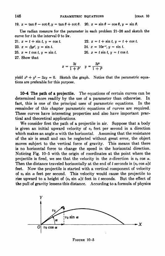
146 PARAMETRIC EQUATIONS [CHAP. 10
19. x = tan cot 0, y = tan 6 + cot 0. 20. x = sin cos 0, y = sin 0.
Use radian measure for the parameter in each problem 21-26 and sketch the
curve for t in the interval to 2ir.
21 . x t + sin ty y = cos t.
23. x = Ae* v = sin J.
25. z = t cos, ?/
= sin t.
27. Show that
22. x
24. x <
26. a:
J + sin t, y = t + cos t.
lOe*1
, ?/= sin t.
t sin t, y = t cos .
3*y
1
yield z3 + y3
3z</= 0. Sketch the graph. Notice that the parametric equa-
tions are preferable for this purpose.
10-4 The path of a projectile. The equations of certain curves can be
determined more readily by the use of a parameter than otherwise. In
fact, this is one of the principal uses of parametric equations. In the
remainder of this chapter parametric equations of curves are required.
These curves have interesting properties and also have important prac-
tical and theoretical applications.
We consider first the path of a projectile in air. Suppose that a bodyis given an initial upward velocity of VQ feet per second in a direction
which makes an angle a with the horizontal. Assuming that the resistance
of the air is small and can be neglected without great error, the object
moves subject to the vertical force of gravity. This means that there
is no horizontal force to change the speed in the horizontal direction.
Noticing Fig. 10-5 with the origin of coordinates at the point where the
projectile is fired, we see that the velocity in the re-direction is VQ cos a.
Then the distance traveled horizontally at the end of t seconds is (v cos a)t
feet. Now the projectile is started with a vertical component of velocity
of VQ sin a feet per second. This velocity would cause the projectile to
rise upward to a height of (t; sin a)t feet in t seconds. But the effect of
the pull of gravity lessens this distance. According to a formula of physics
FIGURE 10-5

10-5] THE CYCLOID 147
the amount to be subtracted is \gP, where g is a constant and approxi-
mately equal to 32. Hence the parametric equations of the path are
x =(i/o cos OL)t> y = (VQ sin oc)t
-%g(*. (1)
If we solve the first equation for t and substitute the result in the second,we get the equation of the path in the rectangular form
y = (tan a)x - /** , (2)y v ' 2vQ2 cos2 a v '
This equation, which is of the second degroe in x and the first degree in?/,
represents a parabola.
KXAMPLK. A stone is thrown upward with a velocity of 100 feet per second
at an angle of -If) with the horizontal. Write the equations of the path in para-
metric and rectangular forms.
Solution. We substitute r = 100, a = 45, and g = 32 in equations (1) and (2).
This gives the parametric equations
j = S0\ :
j/, //= SO\ /:
J/ - 16f2,
and the rectangular equation
.r2
IJ~ x ~"
sTxT
This last equation, reduced to standard form, becomes
(j - 100)- = -S00(// - 200).
The vertex, at (400.200), is the highest point reached by the stone. Setting
//=
0, we find j = SOO. Hence the stone strikes the ground at the point (S00,0).
10-5 The cycloid. The path traced by a given point on the circum-
ference of a circle which rolls along a lino is called a cycloid. In order to
derive the equation of the cycloid, we select the line as the .r-axis and take
the origin at a position where the tracing point is in contact with the
.r-axis.
In Fig. 10-0 the radius of the rolling circle is a, and P is the tracing
point. In the position drawn, the circle has rolled so that CP makes an
angle (radians) with the vertical. Having rolled without slipping, the
segment OB and the arc PR are of equal length. Hence
OB = arc PB = aB.
Noticing the right triangle PDC, we may write
.r = 0.4 =OB-PD = ae-a sin 0,
y = AP = BC - DC = a - a cos 6.
The equations of the cycloid in parametric form are
x = a(0 - sin 9), y = a(l - cos 0).

148 PARAMETRIC EQUATIONS [CHAP. 10
FIGURE 10-6
The result of eliminating from these equations is the complicated equation
x = a arc cos =fc V2 ay-
y*.
EXERCISE 10-2
1. A ball is thrown upward with an initial velocity of 80 feet per second at
an angle of 45 with the horizontal. Write the parametric equations of its path,
using g - 32. Find also the rectangular equation of the path. How high does
the ball ascend and how far away, assuming the ground level, does it strike the
ground?
2. A projectile is fired upward with a velocity of 160 feet per second at an
angle of 30 with the horizontal. Find the coordinates of its position at the end
of (a) 1 second, (b) 3 seconds, (c) 5 seconds. At what times is the projectile
64 feet above the starting point?
3. Write the equations, both in parametric and rectangular forms, of the
path of a projectile which is fired horizontally with a velocity of t; feet per second.
If the projectile is fired horizontally from a building 64 feet high, find how far
downward and how far horizontally it travels in 2 seconds.
4. A circle of radius a roils along a line. A point on a radius, 6 units from
the center, describes a path. Paralleling the derivation in Section 10-5, show
that the path is represented by the equations
x = ad 6 sin 0, y = a b cos 6
The curve is called a curtate cycloid if 6 < a and a prolate cycloid if 6 > a.
5. Sketch the curve of the equations in problem 4, taking a = 4 and 6 = 3.
Sketch the curve if a = 4 and 6 = 6.
6. A circle of radius 4 rolls along a line and makes a revolution in 2 seconds.
A point, starting downward on a vertical radius, moves from the center to the cir-
cumference along the radius at a rate of 2 feet per second. Find the equations
of the path of the point.
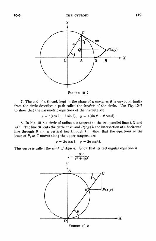
10-5] 149
FIGURE 10-7
7. The end of a thread, kept in the plane of a circle, as it is unwound tautly
from the circle describes a path called the involute of the circle. Use Fig. 10-7
to show that the parametric equations of the involute are
x = a(cos + Q sin 6), y = a(sin 6 6 cos 0).
8. In Fig. 10- -8 a circle of radius a is tangent to the two parallel lines OX and
AC. The line OC cuts the circle at B, and P(x,y) is the intersection of a horizontal
line through B and a vertical line through C. Show that the equations of the
locus of Ptas C moves along the upper tangent, are
x = 2a tan 0, y = 2a cos2 0.
This curve is called the witch of Agncsi. Show that its rectangular equation is
OFIGURE 10-8

150 PARAMETRIC EQUATIONS [CHAP. 10
FIGURE 10-9
9. In Fig. 10-9, OP = AB. Show that the equations of the path traced by P,
as A moves around the circle, are
x = 2o sin26, y = 2a sin2 tan 0.
The curve is called the dssoid of Diodes. The rectangular equation is
10. The path traced by a given point on the circumference of a circle of radius
Jtt as it rolls inside and along a circle of radius a is called a hypocydoid of four
cusps. Use Fig. 10-10 to obtain the parametric equations
x - a cos30, y - a sin3
6.
Y
FIGURE 10-10
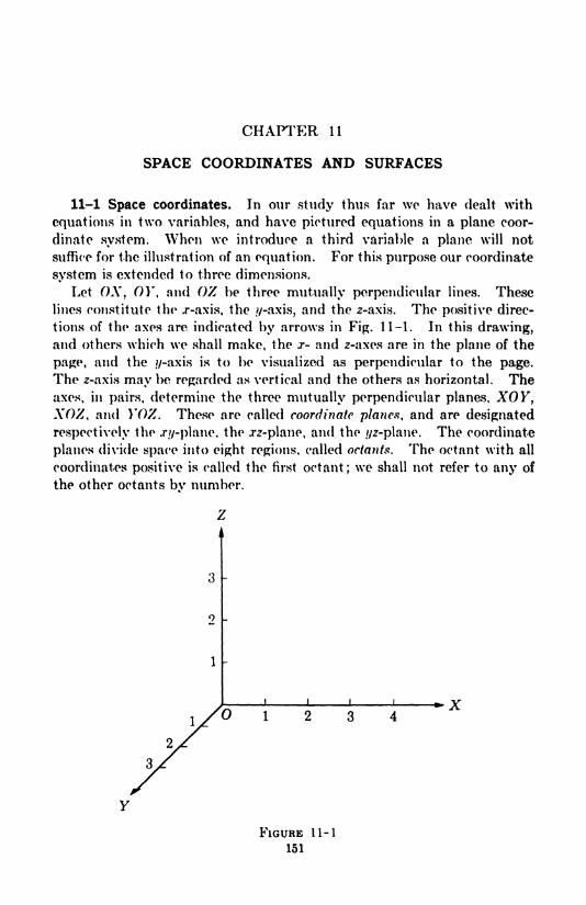
CHAPTER 11
SPACE COORDINATES AND SURFACES
11-1 Space coordinates. In our study thus far wo have dealt with
equations in two variables, and have pictured equations in a plane coor-
dinate system. When we introduce a third variable a plane will not
suffice for the illustration of an equation. For this purpose our coordinate
system is extended to three dimensions.
Let OA", 01", and OZ be three mutually perpendicular lines. These
lines constitute the .r-axis, the //-axis, and the 2-axis. The positive direc-
tions of the axes are indicated by arrows in Fig. 11-1. In this drawing,and others which we shall make, the j- and 2-axes are in the plane of the
page, and the //-axis is to be visualized as perpendicular to the page.
The 2-axis may be regarded as vertical and the others as horizontal. The
axes, in pairs, determine the three mutually perpendicular planes, XOY,XOZ, and YOZ. These are called coordinate planes, and are designated
respectively the .r//-plane. the .rz-plane, and the //z-plane. The coordinate
planes divide space into eight regions, called octants. The octant with all
coordinates positive is called the first octant; we shall not refer to any of
the other octants bv number.
'O I
X
FIGURE 11-1
151
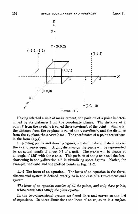
152 SPACE COORDINATES AND SURFACES
z
[CHAP. 11
(-1.5.-1,]
-(0,0,2)
(3,1,2)
f(0,2,0)
*(2,0,-2)
FIGURE 11-2
Having selected a unit of measurement, the position of a point is deter-
mined by its distances from the coordinate planes. The distance of a
point P from the f/z-plane is called the x-coordinatc of the point. Similarly,
the distance from the zz-plane is called the y-coordinate, and the distance
from the rr?/-plane the z-coordinate. The coordinates of a point are written
in the form (x,y,z).
In plotting points and drawing figures, we shall make unit distances on
the x- and z-axes equal. A unit distance on the */-axis will be represented
by an actual length of about 0.7 of a unit. The y-axis will be drawn at
an angle of 135 with the z-axis. This position of the //-axis and the fore-
shortening in the ^-direction aid in visualizing space figures. Notice, for
example, the cube and the plotted points in Fig. 11-2.
11-2 The locus of an equation. The locus of an equation in the three-
dimensional system is defined exactly as in the case of a two-dimensional
system.
The locus of an equation consists of all the points, and only those points,
whose coordinates satisfy the given equation.
In the two-dimensional system we found lines and curves as the loci
of equations. In three dimensions the locus of an equation is a surface.
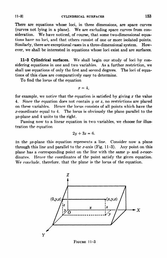
11-3] CYLINDRICAL SURFACES 153
There are equations whose loci, in three dimensions, are space curves
(curves not lying in a plane). We are excluding space curves from con-
sideration. We have noticed, of course, that some two-dimensional equa-tions have no loci, and that others consist of one or more isolated points.
Similarly, there are exceptional cases in a three-dimensional system. How-
ever, we shall be interested in equations whose loci exist and are surfaces.
11-3 Cylindrical surfaces. We shall begin our study of loci by con-
sidering equations in one and two variables. As a further restriction, weshall use equations of only the first and second degrees. The loci of equa-tions of this class are comparatively easy to determine.
To find the locus of the equation
for example, we notice that the equation is satisfied by giving x the value
4. Since the equation does not contain ?/ or z, no restrictions are placed
on these variables. Hence the locus consists of all points which have the
^-coordinate equal to 4. The locus is obviously the plane parallel to the
?/2-plane and 4 units to the right.
Passing now to a linear equation in two variables, we choose for illus-
tration the equation
2y + 3z = 6.
In the ^-plane this equation represents a line. Consider now a plane
through this line and parallel to the x-axis (Fig. 11-3). Any point on this
plane has a corresponding point on the line with the same //- and ^-coor-
dinates. Hence the coordinates of the point satisfy the given equation.
We conclude, therefore, that the plane is the locus of the equation.
FIGURE 11-3
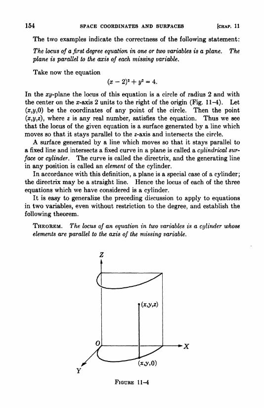
154 SPACE COORDINATES AND SURFACES [CHAP. 11
The two examples indicate the correctness of the following statement:
The locus of a first degree equation in one or two variables is a plane. The
plane is parallel to the axis of each missing variable.
Take now the equation
(x-
2)2 + y*
- 4.
In the xy-plane the locus of this equation is a circle of radius 2 and with
the center on the ar-axis 2 units to the right of the origin (Fig. 11-4). Let
(z,2/,0) be the coordinates of any point of the circle. Then the point
(x,y,z), where z is any real number, satisfies the equation. Thus we see
that the locus of the given equation is a surface generated by a line which
moves so that it stays parallel to the z-axis and intersects the circle.
A surface generated by a line which moves so that it stays parallel to
a fixed line and intersects a fixed curve in a plane is called a cylindrical sur-
face or cylinder. The curve is called the directrix, and the generating line
in any position is called an element of the cylinder.
In accordance with this definition, a plane is a special case of a cylinder;
the directrix may be a straight line. Hence the locus of each of the three
equations which we have considered is a cylinder.
It is easy to generalize the preceding discussion to apply to equationsin two variables, even without restriction to the degree, and establish the
following theorem.
THEOREM. The locus of an equation in two variables is a cylinder whose
elements are parallel to the axis of the missing variable.

11-4] THE GENERAL LINEAR EQUATION 155
EXERCISE 11-1
1. Draw the coordinate axes and plot the points: 4(0,0,2), 5(0,2,0), C(2,0,0),
D(2,3,0), (3,2,4), ^(-2,0,4), <?(-!,-!, -1), //(2,l,-2).
2. Draw a cube which has the origin and the point (4,4,4) as opposite corners.
Write the coordinates of the other corners.
3. Draw the edges of a box which has four of its vertices located at the points
(0,0,0), (3,0,0), (0,2,0), and (0,0,2). Write the coordinates of the other vertices.
4. Draw the rectangular parallelepiped which has three of its faces in the
coordinate planes and the points (0,0,0) and (4,5,3) as the ends of a diagonal.
Write the coordinates of the vertices.
Describe the surface corresponding to each equation 5-24 and make a sketch
of the surface.
5. x = 0. f>. //= 0. 7. 2 = 0.
S. 2 = 5. 9. 2 = -5. 10. i + //= 4.
11. 3-r + \z = 12. 12. 2// + 2 = 0. 13. x -+ 2 = 0.
14. 2x -//= 0. 15. 3// -2 = 6. If), z - 4x = S.
17. j.2 + V2 = 4. IS. (//
-2)
2 + 22 = 1. 19. r2 = 92.
20. ir= 42. 21. (.r
-2)
2 = %. 22. 4x* + 9//2 = 36.
23. J2 + 22 - 4j -6// + 9 = 0. 24. j- + 4//
2 - 4* -32y/
= 64.
11-4 The general linear equation. In rectangular coordinates of two
dimensions we found that a linear equation, in either one or two variables,
represents a line. In our three-dimensional system we might, by analogy,
surmise that linear equations, in one, two, or three variables, represent
surfaces of the same type. The surmise is correct. At this point, how-
ever, we merely state the fact as a theorem, and reserve the proof for the
next chapter.
THKORKM. The locus, in three dimensions, of the equation
Ax + BI/ + CZ + D = 0,
where A, 7?, and C are not all zero, is a plane.
The location of a plane represented by a linear equation can be deter-
mined by finding the lines in which the plane intersects the coordinate
planes. These intersections, as well as the intersections which any sur-
face makes with the coordinate planes, are called traces.
Consider the equation
4x + 3y + 6z = 12.
The trace of the locus on the arc-plane has the ^-coordinate equal to zero.
Hence we set y = in the given equation and have
4jr + 6* - 12

156 SPACE COORDINATES AND SURFACES [CHAP. 11
z
C(0,0,2)
3y + 62 = 12
FIGURE 11-5
as the equation of the trace on the zz-plane. The equations of the traces
on the xy- and i/z-planes are
4z + 3y = 12 and 3y + 62 = 12.
Figure 11-5 shows segments of the traces. These segments form a triangle
which may be used to picture the plane.
11-6 Second degree equations. The locus of a second degree equation
is called a quadric surface. In general it is not easy to determine the
characteristics and location of a quadric surface corresponding to an
equation. We shall use equations of simple type, however, whose loci are
more easily studied.
The main device in examining the locus of an equation consists in ob-
serving the intersections of the surface by the coordinate planes and planes
parallel to them. The idea of symmetry, as in a two-dimensional system,
can be used to advantage. If x can be replaced by x without changing
the equation, there is symmetry with respect to the $/2-plane. Similar
statements apply for the other variables and coordinate planes.
To illustrate the method, we examine the equation
X2 + 7/2 = Z.
The surface is symmetric with respect to the yz- and rrz-planes. Negativevalues must not be assigned to z. This tells us that no part of the surface
is below the zt/-plane. When z =0, x = and y = 0. Sections made by
planes parallel to the xy-plane are circles. This is evident if we substitute
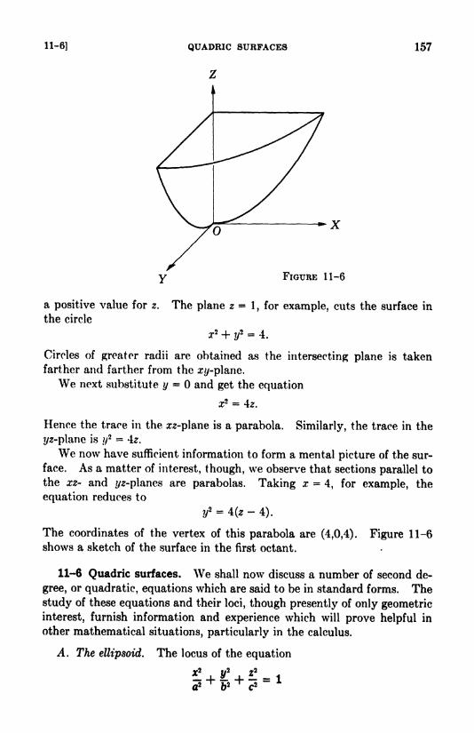
11-6] QUADRIC SURFACES 157
FIGURE 11-6
a positive value for z. The plane z = 1, for example, cuts the surface in
the circle
r2 + ?/= 4.
Circles of greater radii are obtained as the intersecting plane is taken
farther and farther from the zt/-plane.
We next substitute y = and get the equation
a:2 = 4z.
Hence the trace in the zz-plane is a parabola. Similarly, the trace in the
t/z-plane is //2 = 4z.
We now have sufficient information to form a mental picture of the sur-
face. As a matter of interest, though, we observe that sections parallel to
the xz- and #z-planes are parabolas. Taking x =4, for example, the
equation reduces to
?/= 4(
-4).
The coordinates of the vertex of this parabola are (4,0,4). Figure 11-6
shows a sketch of the surface in the first octant.
11-6 Quadric surfaces. We shall now discuss a number of second de-
gree, or quadratic, equations which are said to be in standard forms. The
study of these equations and their loci, though presently of only geometric
interest, furnish information and experience which will prove helpful in
other mathematical situations, particularly in the calculus.
A. The ellipsoid. The locus of the equation
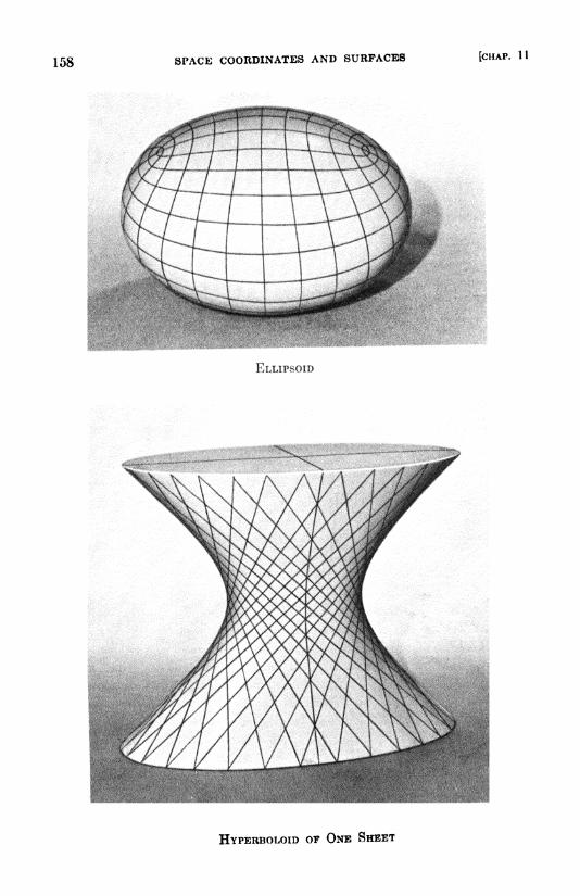
158 SPACE COORDINATES AND SURFACES [CHAP. 11
ELLIPSOID
HYPERBOLOID OF ONE SHEET
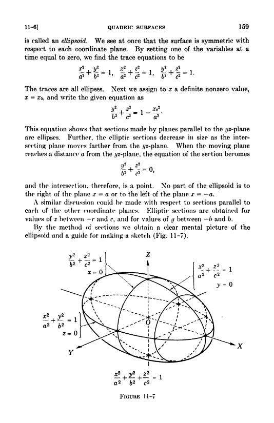
11-6] QUADRIC SURFACES 159
is called an ellipsoid. We see at once that the surface is symmetric with
respect to each coordinate plane. By setting one of the variables at a
time equal to zero, we find the trace equations to be
The traces are all ellipses. Next we assign to x a definite nonzero value,
x =0*0, and write the given equation as
b2'
c2
This equation shows that sections made by planes parallel to the ?/-plane
are ellipses. Further, the elliptic sections decrease in size as the inter-
secting plane moves farther from the /ye-plane. When the moving planereaches a distance a from the //z-plane, the equation of the section becomes
and the intersection, therefore, is a point. No part of the ellipsoid is to
the right of the plane jc = a or to the left of the plane -r = a.
A similar discussion could be made with respect to sections parallel to
each of the other coordinate planes. Elliptic sections are obtained for
values of z between r and r, and for values of y between b and 6.
By the method of sections we obtain a clear mental picture of the
ellipsoid and a guide for making a sketch (Fig. 11-7).
2 52 C2
FIGURE 1 1-7
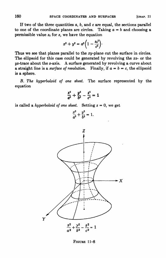
160 SPACE COORDINATES AND SURFACES [CHAP. 11
If two of the three quantities a, 6, and c are equal, the sections parallel
to one of the coordinate planes are circles. Taking a = b and choosing a
permissible value ZQ for 2, we have the equation
Thus we see that planes parallel to the zy-plane cut the surface in circles.
The ellipsoid for this case could be generated by revolving the xz- or the
i/2-trace about the z-axis. A surface generated by revolving a curve about
a straight line is a surface of revolution. Finally, if a = b = c, the ellipsoid
is a sphere.
B. The hyperboloid of one sheet. The surface represented by the
equation
*! + l!.
2
_*! = i
a2""
&2 c2
is called a hyperboloid of one sheet. Setting z = 0, we get
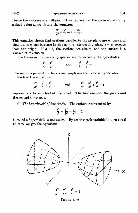
11-6] QUADRIC SURFACES 161
Hence the xy-trace is an ellipse. If we replace z in the given equation bya fixed value z
,we obtain the equation
This equation shows that sections parallel to the zt/-plane are ellipses and
that the sections increase in size as the intersecting plane z - zo recedes
from the origin. If a = 6, the sections are circles, and the surface is a
surface of revolution.
The traces in the xz- and i/z-planes are respectively the hyperbolas
*2 *2i j 2/
2 *i-i- -5
= 1 and =--^= 1.
a2 c2 o2 c2
The sections parallel to the xz- and 7/z-planes are likewise hyperbolas.
Each of the equations
?'_?/! + 5? =]a2 62 c2
and
represents a hyperboloid of one sheet. The first encloses the #-axis and
the second the r-axis.
C. The hypcrholoid of two sheets. The surface represented by
_ !_ !- i
a2 b2 c2
is called a hyperboloid of (wo sheets. By setting each variable in turn equal
to zero, we get the equations
a2 62 C2
FIGURE 11-9
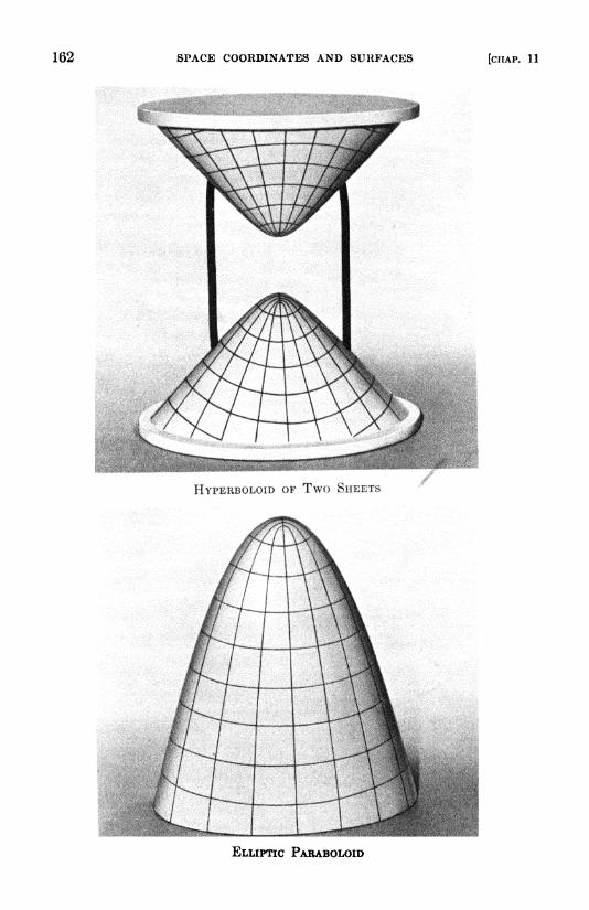
162 SPACE COORDINATES AND SURFACES [CHAP. 11
HYPERBOLOID OF Two SHEETS
ELLIPTIC PARABOLOID

11-6]
xla2
QUADRIC SURFACES
.,1 ?!-!=! -^
163
The first two equations show that the xy- and zz-traces are hyperbolas.
The third tells us there is no trace in the 7/z-plane. The sections made
by the plane x = XQ is given by the equation
This equation represents a point or an ellipse according as the numerical
value of J is equal to or greater than a. Sections parallel to the xz- and
r/y-planes are hyperbolas. From this information the surface (Fig. 11-9)
is readily visualized.
If b =r, the hyperboloid of two sheets is a surface of revolution.
Hyporboloids of two sheets are also represented by the equations
a- 0- cz a2 62 c
D. T/jf elliptic paraboloid. The locus of the equation
FIGURE 11-10
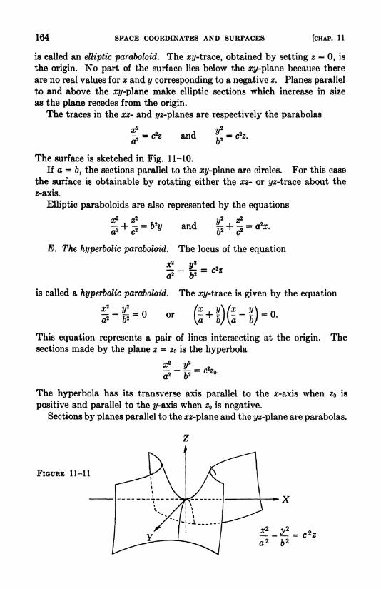
164 SPACE COORDINATES AND SURFACES [CHAP. 11
is called an elliptic paraboloid. The zy-trace, obtained by setting z = 0, is
the origin. No part of the surface lies below the z,y-plane because there
are no real values for x and y corresponding to a negative z. Planes parallel
to and above the :rt/-plane make elliptic sections which increase in size
as the plane recedes from the origin.
The traces in the xz- and i/z-planes are respectively the parabolas
~~7j*" c z and ~7~n
~ c z.a2 o2
The surface is sketched in Fig. 11-10.
If a = bj the sections parallel to the zz/-plane are circles. For this case
the surface is obtainable by rotating either the xz- or i/z-trace about the
z-axis.
Elliptic paraboloids are also represented by the equations
E. The hyperbolic paraboloid. The locus of the equation
^-^
= C2z
is called a hyperbolic paraboloid. The xy-tr&cQ is given by the equation
~~o~~"
jTiz
= " Or I r |" 1 1 va o \a o/ \a u
This equation represents a pair of lines intersecting at the origin. Thesections made by the plane z = z is the hyperbola
2 -,,2
The hyperbola has its transverse axis parallel to the x-axis when z is
positive and parallel to the i/-axis when z is negative.
Sections by planes parallel to the zz-plane and the t/z-plane are parabolas.
FIGURE 11-11
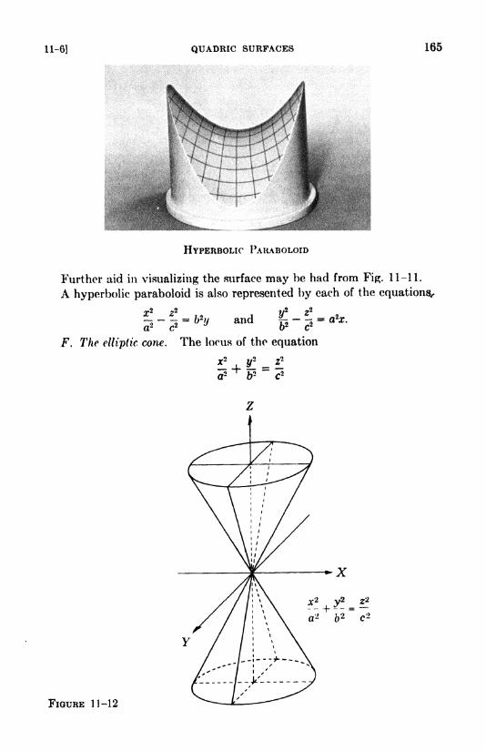
11-6] QUADRIC SURFACES 165
HYPERBOLIC PARABOLOID
Further aid in visualizing the surface may be had from Fig. 11-11.
A hyperbolic paraboloid is also represented by each of the equations^
/2 ~2 7/2 yl
F. The elliptic cone. The locus of the equation
FIGURE 11-12
166 SPACE COORDINATES AND SURFACES [CHAP. 11
is an elliptic cone. Setting z, ?/, and z in turn equal to zero, we have the
trace equations
a? 3/2 ?!-?! ^^5!a2
"i
~62~ U
' a2 c2'
62 c2'
These equations reveal that the x?/-trace is the origin, and that each of the
other traces is a pair of lines intersecting at the origin.
Sections parallel to the #z/-plane are ellipses, and those parallel to the
other coordinate planes are hyperbolas.
For the case in which a = 6, the cone is a right circular cone.
Elliptic cones are also represented by the equations
EXERCISE 11-2
Draw the traces on the coordinate planes:
1. 2x + 3y + 4z = 12. 2. 2x + y + 2z = 4.
3. x - 4?/ + z = 4. 4. 2x + 3f/- z = 6.
5. x + t/ 2 = 0. 6. x ?/= 0.
Identify and sketch each quadric surface. If preferred, make the sketch in
the first octant only and state the symmetry with respect to the coordinate planes:
9. x2 + z/2 + 22 = 16. 10.
13. a;2 + y
- zz = 16. 14. z2 -y2 - z2 = 16.
15 El _ t - * - 1 i ^ _ f _ L2
_ 11S<16 9 4
~ L 16 '
4 9 9~ L
19. y* + z* = 4x. 20. a;2 -
y*= 4z.
9 16~
4''
4~
4
23 5l + ^ = l2
. 24 ^ + ?-2
'
16^
9 4^'
4+
4
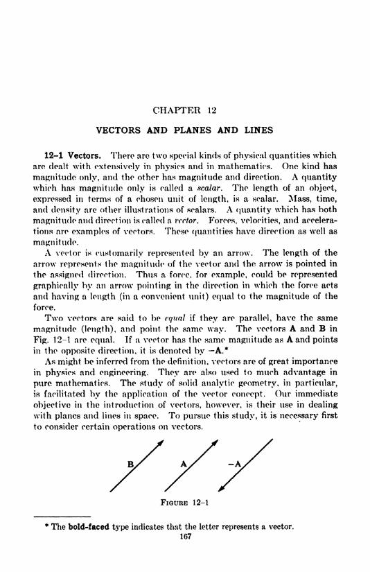
CHAPTER 12
VECTORS AND PLANES AND LINES
12-1 Vectors. There are two special kinds of physical quantities which
are dealt with extensively in physics and in mathematics. One kind has
magnitude only, and the other has magnitude and direction. A quantitywhich has magnitude only is called a scalar. The length of an object,
expressed in terms of a chosen unit of length, is a scalar. Mass, time,
and density are other illustrations of scalars. A quantity which has both
magnitude and direction is called a rector. Forces, velocities, and accelera-
tions are examples of vectors. These quantities have direction as well as
magnitude.A vector is customarily represented by an arrow. The length of the
arrow represents the magnitude of the vector and the arrow is pointed in
the assigned direction. Thus a force, for example, could be represented
graphically by an arrow pointing in the direction in which the force acts
and having a length (in a convenient unit) equal to the magnitude of the
force.
Two vectors are said to be equal if they are parallel, have the same
magnitude (length), and point the same way. The vectors A and B in
Fig. 12-1 are equal. If a vector has the same magnitude as A and points
in the opposite direction, it is denoted by A.*
As might be inferred from the definition, vectors are of great importancein physics and engineering. They are also used to much advantage in
pure mathematics. The study of solid analytic geometry, in particular,
is facilitated by the application of the vector concept. Our immediate
objective in the introduction of vectors, however, is their use in dealing
with planes and lines in space. To pursue this study, it is necessary first
to consider certain operations on vectors.
FIGURE 12-1
* The bold-faced type indicates that the letter represents a vector.
167
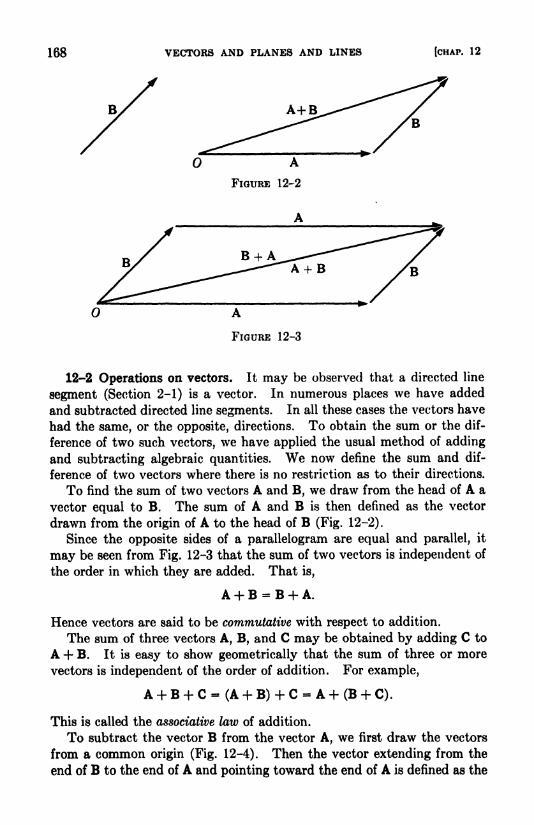
168 VECTORS AND PLANES AND LINES
A+B
[CHAP. 12
12-2 Operations on vectors. It may be observed that a directed line
segment (Section 2-1) is a vector. In numerous places we have added
and subtracted directed line segments. In all these cases the vectors have
had the same, or the opposite, directions. To obtain the sum or the dif-
ference of two such vectors, we have applied the usual method of adding
and subtracting algebraic quantities. We now define the sum and dif-
ference of two vectors where there is no restriction as to their directions.
To find the sum of two vectors A and B, we draw from the head of A a
vector equal to B. The sum of A and B is then defined as the vector
drawn from the origin of A to the head of B (Fig. 12-2).
Since the opposite sides of a parallelogram are equal and parallel, it
may be seen from Fig. 12-3 that the sum of two vectors is independent of
the order in which they are added. That is,
A + B = B + A.
Hence vectors are said to be commutative with respect to addition.
The sum of three vectors A, B, and C may be obtained by adding C to
A + B. It is easy to show geometrically that the sum of three or more
vectors is independent of the order of addition. For example,
A + B + C = (A + B) + C - A + (B + C).
This is called the associative law of addition.
To subtract the vector B from the vector A, we first draw the vectors
from a common origin (Fig. 12-4). Then the vector extending from the
end of B to the end of A and pointing toward the end of A is defined as the

12-3] VECTORS IN A RECTANGULAR COORDINATE PLANE 169
A-B
FIGURE 12-5
difference A B. The triangle formed by the vectors B, A B, and Ashows that
B + (A-
B) - A.
That is, A B is the vector which added to B gives A.
The product of a scalar m and a vector A, expressed by ??iA, is a vector
m times as long as A, and has the direction of A if m is positive, and the
opposite direction if m is negative. If m = 0, the product is a zero vector.
If m = -1, the product is -A. (See Fig. 12-5.)
If m and n are scalars, the sum of wA and wA is a vector m + n times
as long as A. This is expressed by
nA = (m + n)A. (1)
The vectors A and B and A + B form the sides of a triangle (Fig. 12-2).
If each of these vectors is multiplied by a scalar m, then wA, ?wB, and
m(A + B) form a similar triangle, and hence
w(A + B) = wA + wB. (2)
Equations (1) and (2) show that vectors and scalars obey the distributive
law of multiplication.
12-3 Vectors in a rectangular coordinate plane. Vectors are con-
veniently dealt with when they are expressed as the sum of vectors parallel
to the coordinate axes. The letters i and j are usually employed to repre-
sent vectors of unit length from the origin to the points (1,0) and (0,1)
respectively. Any vector in the plane can be expressed as the sum of a
scalar times i and a scalar times j. Thus the vector V (Fig. 12-0) may be
written as
V = ai + 6j.
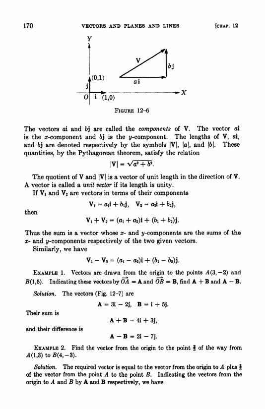
170 VECTORS AND PLANES AND LINES [CHAP. 12
yi,
1(0,1)
* (1,0)
FIGURE 12-6
The vectors ai and bj are called the components of V. The vector ai
is the z-component and bj is the ^/-component. The lengths of V, ai,
and bj are denoted respectively by the symbols |V|, |a|, and |6|. These
quantities, by the Pythagorean theorem, satisfy the relation
The quotient of V and |V| is a vector of unit length in the direction of V.
A vector is called a unit vector if its length is unity.
If Vi and V2 are vectors in terms of their components
i- aii + a2i +
then
Vt + V2-
(01 + ai)i + (61 + 6i)j.
Thus the sum is a vector whose x- and ^/-components are the sums of the
x- and ^-components respectively of the two given vectors.
Similarly, we have
V1 -V2 =(a1 -o2)i+(& 1 -62)j.
EXAMPLE 1. Vectors are drawn from the origin to the points A (3, 2) and
5(1,5). Indicating these vectors by OA = A and OB = B, find A + B and A - B.
Solution. The vectors (Fig. 12-7) are
A = 3i - 2j, B * i + 5j.
Their sum is
A + B = 4i + 3j,
and their difference is
A - B = 2i - 7j.
EXAMPLE 2. Find the vector from the origin to the point of the way from
A(l f3)toB<4,-3).
Solution. The required vector is equal to the vector from the origin to A plus $
of the vector from the point A to the point B. Indicating the vectors from the
origin to A and B by A and B respectively, we have

12-3] VECTORS IN A RECTANGULAR COORDINATE PLANE
Y
171
(4,3)
FIGURE 12-7
A = i + 3j,
B = 4i - 3j,
B - A = 3i - 6j.
Hence the required vector V is
V = i + 3j + (3i-
6j)= 3i - j.
EXERCISE 12-1
In problems 1-4 find the sum of the vectors from the origin to the given points.
Also subtract the second vector from the first. Draw all vectors.
1. .4(2,3), #(-4,5).3. 4 (3, -2), B(-i,-4).
2. 4(5,0), 5(0,4).
4. 4(6,7), B(-5,-5).
Determine a unit vector having the direction of the vector in each problem 5-8.
5. 3i + 4j. 6. 3i - 12j. 7. 12i - 5j.
8. 2i - 3j. 9. i + 2j. 10. 4i + 3j.
Find the length of each vector 9-12 and the cosine of the angle which the
vector makes with the positive z-axis.
11. i + j. 12. -i + 3j. 13. i+Oj.
14. Oi + 3j. 15. -3i + 2j. 16. 5i + 12j.
17. Find the vector from the origin to the mid-point of the vector PiP2 join-
ing P,(3,8) and P2(5,- 8).

172 VECTORS AND PLANES AND LINES [CHAP. 12
18. Find the vectors from the origin to the trisection points of the vector PiP 2
joining the points Pi(-3,4) and P2(12,-5).
12-4 Vectors in space. In the three-dimensional rectangular coordinate
system the unit vectors from the origin to the points (1,0,0), (0,1,0), and
(0,0,1) are denoted respectively by i, j, and k. Any vector in space can
be expressed in terms of these unit vectors. Thus the vector from the
origin to the point A (a,b,c) is
OA = A - ai + 6j + ck.
The vectors ai, bj, and ck are the x-, t/-, and z-components of the vector A.
The length of the vector A may be obtained by using the lengths of the
sides of the right triangles OCA and ODC (Fig. 12-8). From the Pythag-orean relation, we have
(OAY - (OC)2 + (CAY
-(OZ>)
2 + (DC)2 + (CAY
= a2 + fc2 + c2 .
Hence the length of A is
62 + c2 .
The vector from Pi(xi,y i9zi) to P^x^y^z^ in Fig. 12-9 has the compo-nents (x<t Xi)i, (7/2
~2/1)j, (22 2i)k. Hence it is expressed by
P\Pt = (*,-
xi)i + (yt-
i/OJ + (*-
zi)k.
The length of the vector PiP2 ,or the distance d between the points Pi and
P2 ,is
FIGURE 12-8

12-4] VECTORS IN SPACE 173
FIGURE 12-0
EXAMPLE. The points .4(1, -2,3), #(-4,5,6), and 0(5,7,0) are vertices of a
triangle. Express the sides as vectors and find the length of each side.
Solution. The vectors from the origin to the given points are
OA = A = i-
2j + 3k,
OB = B = -4i + 5j -f 6k,
OC = C = 5i + 7j.
The sides, expressed as vectors, are
AB = B - A = -5i -f 7j 4- 3k,
BC = C - B = 9i + 2j-
6k,
CA = A - C - -4i -9j -f 3k.
The lengths of the vectors are
\AB\ = V(-5yr+~72~+l? = v'S3,
\Bc\ =
\CA\ =
22 + (-6) 2 =11,
)*+ (-9>-h3 2 = Vl06.
EXERCISE 12-2
Find the distance between the points A and B in each problem 1-4.
1. A(-3,2,0), #(6,-4,2). 2. .4(3,1,4), B(l f-l
f -2).
3. A(5,7,l), 5(6,-3,2). 4. .4(4,4,0), 5(-2,l,-2).
In each problem 5-8 the given points are the vertices of a triangle. Determine
the vectors AB, BC, and CA and the lengths of these vectors.
5. A(6,8,l),(0,2,l),C(0,-4,-5).

174 VECTORS AND PLANES AND LINES [CHAP. 12
6.
7. A(3,3,3), 8(4,5,5), C(l,2,5).
8. .1(2,4,5), B(6,8,-l), C(-2,-2,l).
Determine a unit vector having the direction of the vector in each problem 9-12.
9. 6i + 3J- 6k. 10. 2i - 4j + 4k.
11. 2i - j- 3k. 12. i + j + k.
13. Find the vectors from the origin to the mid-point and the trisection points
of the line segment (1, 3,7), (7,3, 2). What are the coordinates of the terminal
points of these vectors?
14. Find the equation of a sphere of radius 5 and center at (1, 2,3).
15. Find the center and radius of the sphere x* + ?/2 + z2 + 4x 2y + fa = 0.
16. Find the coordinates of the points which divide the line segment (4,5,7),
(2,3,5) into four equal parts.
17. Find the vector from the origin to the intersection of the medians of the
triangle whose vertices are 4(4,2,1), J5( 5,7,0), and C(4, 3,5).
18. The line segment (3,4,6), ( 1,1,0) is produced by its own length througheach end. Find the coordinates of the new ends.
12-5 The scalar product of two vectors. So far we have not defined a
product of two vectors. Actually there are two kinds of products of two
vectors which have arisen in physics and are extensively used. We shall
define one of these products and make some applications to geometry.The scalar product of two vectors A and B, denoted by A B, is defined
by the equation
A-B= |A||B|cos0,
where 6 is the angle between the vectors when drawn from a commonorigin (Fig. 12-10). It makes no difference whether 6 is taken as positive
or negative, since cos 6 = cos (-6). However, we shall restrict B to the
range from to 180. The angle 6 is if A and B point in the same
direction, and is equal to 180 if they point oppositely. The name scalar
is used because the product is a scalar quantity. This product is also
called the dot product, since the product is indicated by placing a dot
between the two vectors.
MFIGURE 12-10

12-51 THE SCALAR PRODUCT OF TWO VECTORS 175
In the figure the point M is the foot of the perpendicular to the vector Adrawn from the point of B. The vector from to M is called the vector
projection of B on A. The vector projection and A point in the same
direction, since is an acute angle. If 9 exceeds 90, then A and the vector
from to M point oppositely. The scalar projection of B on A is defined
as |B |cos B. The sign of the scalar projection depends on cos 0. Using
the idea of scalar projection of one vector on another, the dot product maybe interpreted geometrically as
A-B =|A| |B|cos0
= (length of A) times (the scalar projection of B on A).
We could also say that the dot product of A and B is the length of B times
the scalar projection of A on B.
It follows immediately from the definition of scalar product that
A-B = B-A. (1)
Hence the dot product of two vectors is said to be commutative.
We next establish the distributive law from the scalar multiplication of
vectors. If we let /> and c stand for the scalar projections of B and C on A,
we see (Fig. 12-1 1) that the sum of the scalar projections of B and C on Ais the same as the scalar projection of (B -4- C) on A. Hence
|A|(6 + c)=
|A|b + |A|c,
and
A (B + C) * A B + A C. (2)
Equation (2) expresses the distributive law for the multiplication of vec-
tors. Since the dot product is commutative [equation (1)], we have also
(B + C) - A = B - A + C - A. (3)
From equations (2) and (3) it maybe seen that the scalar product of two
sums of vectors may be carried out as in multiplying two algebraic ex-
pressions, each of which consists of more than one term. Thus, for
example,
B
Ob c
FIGURE 12-11

176 VECTORS AND PLANES AND LINES [CHAP. 12
If two vectors are expressed in terms of i, j, and k, the scalar productcan be found in a simple way. Let the vectors A and B be expressed as
A = aii + a2j + a3k,
B = M + 62j + 63k.
To obtain the dot product of A and B, we first determine the dot products
of the unit vectors i, j, and k. We have
l-i-J-J-k-k-i,i-j-j-k-k-i-O.
Hence we obtain
A B = aibi + 02&2 + a363 . (4)
Equation (4) shows that the dot product is obtained by the simple process
of adding the products of the corresponding coefficients of i, j, and k.
Since cos 90 = and cos =1, it is evident that the scalar product of
two perpendicular vectors is zero, and the scalar product of two vectors
in the same direction is the product of their lengths. The dot product of a
vector on itself is the square of the length of the vector. That is,
A A =|A|
2.
EXAMPLE 1. Determine whether the vectors
A = 3i + 4j-
8k,
B = 4i - 7j- 2k
are perpendicular.
Solution. The scalar product is
A - B = 12 - 28 + 16 = 0.
Since this product is zero, the vectors are perpendicular.
EXAMPLE 2. Vectors are drawn from the origin to the points 4(6, 3,2) and
B(- 2, 1 ,2) . Find the angle AOB.
Solution. Indicating OA by A and OB by B, we write
A = 6i - 3j + 2k,
B = -2i + j + 2k.
To find the angle, we substitute in both members of the equation
A - B =|A| |B| cos 6.
The product in the left member is A B = -12 - 3 + 4 = -11. The lengths
of A and B are |A|= \/36 + 9 + 4 -
7, |B|= \/4 + 1 + 4 = 3. Hence
--jfrfi-T-
6 = cos-1 = 122 (nearest degree).
12-5] THE SCALAR PRODUCT OP TWO VECTORS 177
EXAMPLE 3. Find the scalar projection and the vector projection of
B = 2i - 3j- k on A = 3i - 6j + 2k.
Solution. The scalar projection of B on A is |B| cos 0, where is the angle
between the vectors. Using the equation
A B = |A||B|cos0,we have
Since A B = 6 + 18 - 2 = 22 and ]A|= V9 + 36 + 4 = 7, it follows that
The scalar projection of B on A is 22 fl'. Since the scalar projection is positive, the
vector projection is in the direction of A. The vector projection is therefore the
product of the scalar projection and a unit vector in the direction of A. This
unit vector is A divided by its length. Hence the vector projection of B on A is
EXERCISE 12-3
Find the dot product of the vectors in each problem 1-4. Find also the cosine
of the angle between the vectors.
1. A = 4i - j + cSk, 2. A = 5i - 3j + 2k,
B = 2i + 2j- k. B = -i + 7j + 13k.
3. A = lOi + 2j + 1 Ik, 4. A = i + j + 2k,
B = 4i - 8j- k. B = Si + 4j + k.
In each problem 5 and G find the scalar projection and the vector projection
of B on A.
5. A = i-
j-
k, 6. A = 3i + 3j + k,
B = lOi - llj + 2k. B = i-
2j- 2k.
7. Find the angle which a diagonal of a cube makes with one of its edges.
8. From a vertex of a cube, a diagonal of a face and a diagonal of, the cube
are drawn. Find the angle thus formed.
The points in problems 9 and 10 are vertices of a triangle. In each determine
the vector from A to B and the vector from A to C. Find the angle between
these vectors. Similarly, find the other interior angles of the triangle.
9. 4(3,4,2), 5(1,7,1), C(-2,3,-5).
10. A(-2,-l,l), (l,0,-2), C(0,-3,l).
11. Let a, /?, and y denote the angles which the vector A = oi + 6j + ck
makes with the positive a>, y-, and z-axes respectively. Using A i, A j, and
A k, find cos a, cos #, and cos 7. The cosines of a, #, and y are called the direc-
tion cosines of the vector A. Show that cos2a. + cos2
ft + cos2 y = 1.
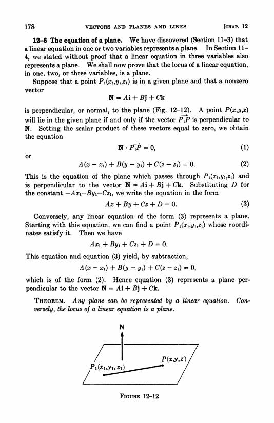
178 VECTORS AND PLANES AND LINES [CHAP. 12
12-6 The equation of a plane. We have discovered (Section 11-3) that
a linear equation in one or two variables represents a plane. In Section 11-
4, we stated without proof that a linear equation in three variables also
represents a plane. We shall now prove that the locus of a linear equation,
in one, two, or three variables, is a plane.
Suppose that a point PI(XI,T/I,I) is in a given plane and that a nonzero
vector
N = Ai + Bj + Ck
is perpendicular, or normal, to the plane (Fig. 12-12). A point P(x,y,z)
will lie in the given plane if and only if the vector P tP is perpendicular to
N. Setting the scalar product of these vectors equal to zero, we obtain
the equation
N PJ> =0, (1)
or
A(x- x,) + B(y - yO + C(z- *) = 0. (2)
This is the equation of the plane which passes through Pi(x\,y\,z\) and
is perpendicular to the vector N = Ai + B] + Ck. Substituting D for
the constant Ax\_ By\ Czi, we write the equation in the form
Ax + By + Cz + D = 0. (3)
Conversely, any linear equation of the form (3) represents a plane.
Starting with this equation, we can find a point Pi(ari,2/i,i) whose coordi-
nates satisfy it. Then we have
Axi + Byi + Czi + D = 0.
This equation and equation (3) yield, by subtraction,
A(x xi) + B(y 1/1) + C(z 21)=
0,
which is of the form (2). Hence equation (3) represents a plane per-
pendicular to the vector N = Ai + Bj + Ck.
THEOREM. Any plane can be represented by a linear equation. Con-
versely, the locus of a linear equation is a plane.
FIGURE 12-12
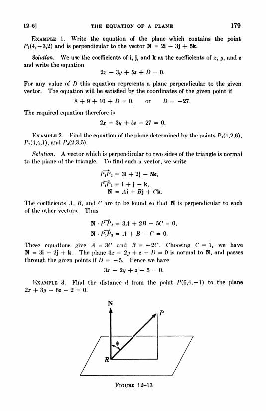
12-6] THE EQUATION OF A PLANE 179
EXAMPLE I. Write the equation of the plane which contains the point
Pi (4, -3,2) and is perpendicular to the vector N = 2i - 3j + 5k.
Solution. We use the coefficients of i, j, and k as the coefficients of x, ?/, and z
and write the equation
2x - 3// + 5* + D = 0.
For any value of D this equation represents a plane perpendicular to the given
vector. The equation will be satisfied by the coordinates of the given point if
8 + 9 + 10 + D =0, or D = -27.
The required equation therefore is
2x - 3// + 62 - 27 = 0.
EXAMPLE 2. Find the equation of the plane determined by the points Pi(l,2,6),
P,(4,4,l),and/>3(2,3,f>).
Solution. A vector which is perpendicular to two sides of the triangle is normal
to the plane of the triangle. To find such a vector, we write
PJ\ = 3i + 2j-
5k,
/VJ3= i + j
-k,
N = Ai + B) + Ok.
The coefficients .1, B, and (T
are to be found so that N is perpendicular to each
of the other vectors. Thus
N 7V> 2= 3.1 + 2B - 50 = 0,
N - /V'a = -1 + B - T = 0.
These equations give A = %C and B = 2C. Choosing 0=1, we have
N = 3i 2j 4- k. The plane 3* 2// -f z + /> = is normal to N, and passes
through the given points if 1) 5. Hence we have
3.r - 2// + z - 5 = 0.
EXAMPLE 3. Find the distance d from the point 7^(6,4, 1) to the plane
2x -f 3/y- 6* - 2 = 0.
FIGURE 12-13
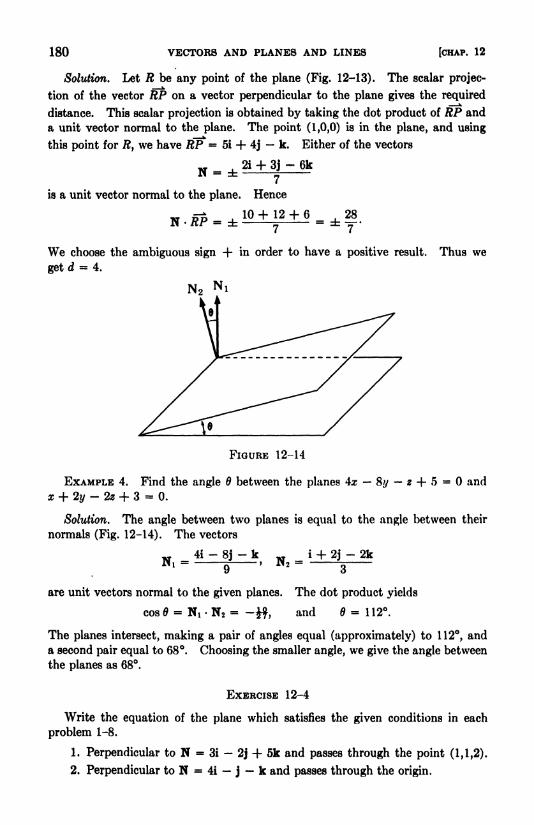
180 VECTORS AND PLANES AND LINES [CHAP. 12
Solution. Let R be any point of the plane (Fig. 12-13). The scalar projec-
tion of the vector HP on a vector perpendicular to the plane gives the required
distance. This scalar projection is obtained by taking the dot product of RP and
a unit vector normal to the plane. The point (1,0,0) is in the plane, and using
this point for R, we have RP = 5i + 4j k. Either of the vectors
N 2i + 3j- 6k- =t
?
is a unit vector normal to the plane. Hence
We choose the ambiguous sign + in order to have a positive result. Thus we
get d = 4.
N 2
FIGURE 12-14
EXAMPLE 4. Find the angle 6 between the planes 4x % 2 + 5 = and
x + 2y- 2z + 3 = 0.
Solution. The angle between two planes is equal to the angle between their
normals (Fig. 12-14). The vectors
w 4i - 8j- k w i + 2j
- 2kN!- J
1 N2= -
are unit vectors normal to the given planes. The dot product yields
cos = N! - N 2= -tf, and = 112.
The planes intersect, making a pair of angles equal (approximately) to 112, and
a second pair equal to 68. Choosing the smaller angle, we give the angle between
the planes as 68.
EXERCISE 12-4
Write the equation of the plane which satisfies the given conditions in each
problem 1-8.
1. Perpendicular to N = 3i - 2j + 5k and passes through the point (1,1,2).
2. Perpendicular to N = 4i - j- k and passes through the origin.

12-7] THE EQUATIONS OF A LINE 181
3. Parallel to the plane 2x 3y 4z = 5 and passes through (1,2, 3).
4. Perpendicular to the line segment (4,0,6), (0, 8,2) at its mid-point.
5. Passes through the origin and is perpendicular to the line through (2, 3,4)
and (5,6,0).
6. Passes through the points (0,1,2), (2,0,3), (4,3,0).
7. Passes through the points (2,-2,-l), (-3,4,1), (4,2,3).
8. Passes through (0,0,0), (3,0,0), (1,1,1).
Find the distance from the given point to the given plane in each problem 9-12.
9. 2z- y + 2z + 3 = 0; (0,1,3).
10. 6x + 2y- 3z + 2 = 0; (2, -4,3).
11. 4x- 2y + 2-2 = 0; (-1,1,2).
12. 3x- 4y- 5z = 0; (5, -1,3).
Find the cosine of the acute angle between each pair of planes in problems 13-16.
13. 2jr + y + * + 3 =0, 2x - 2y + z - 7 = 0.
14. 2x + // + 2z - 5 =0, 2x - 3y + Qz + 5 = 0.
15. 3j - 2y + z - 9 =0, x - 3y
- $z + 4 = 0.
16. j - 8// + 4 - 3 =0, 4j + 2y - 4z + 3 = 0.
17. Show that the planes
A }* + B,?/ + dz + D, =
.4 2:t + 2/y + r2* + D, =
are perpendicular if and only if
jMj + BA + fA = 0.
IS. Determine the value of C so that the planes 2x 6i/ -f Cz = 5 and
x 3v + 2z = 4 are perpendicular.
19. Use vectors to show that the distance d from Pi(opi,yi,*i) to the plane
Ax + /?// -f Tz + D = is
12-7 The equations of a line. Let L be a line which passes through a
given point Pi(xi,y^z\) and is parallel to a given nonzero vector
If P(x,y,z) is a point on the line, then the vector PiP is parallel to V
(Fig. 12-15). Conversely, if P\P is parallel to V, the point P is on the line
L. Hence P is on L if and only if there is a scalar t such that
or
(x-
xi)i +(y- 2/i)j + (*~
zi)k- AA + Btj + CQn. (1)
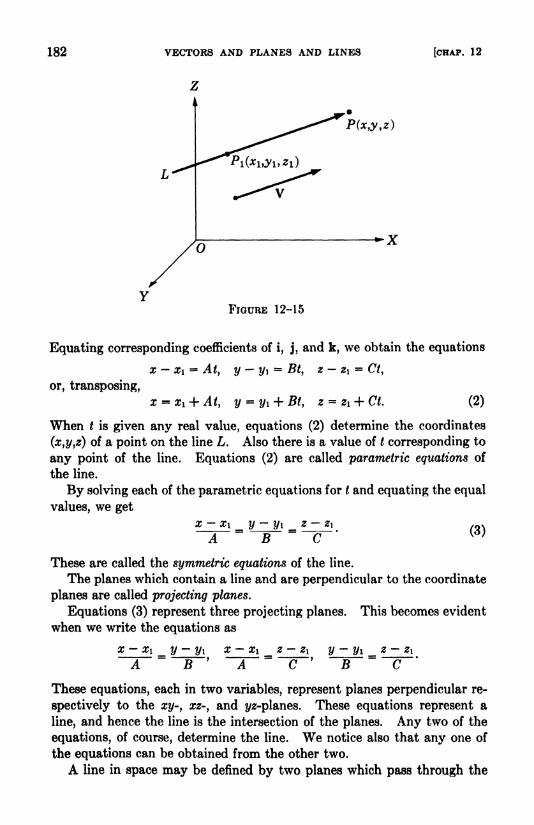
182 VECTORS AND PLANES AND LINES [CHAP. 12
FIGURE 12-15
Equating corresponding coefficients of i, j, and k, we obtain the equations
x - Xi = At, y - y^= Bt, z- z\ = Ct,
or, transposing,
At, (2)
When is given any real value, equations (2) determine the coordinates
(x,y,z) of a point on the line L. Also there is a value of / corresponding to
any point of the line. Equations (2) are called parametric equations of
the line.
By solving each of the parametric equations for t and equating the equal
values, we get
x - xi y-
t/i z-z\B a (3)
These are called the symmetric equations of the line.
The planes which contain a line and are perpendicular to the coordinate
planes are called projecting planes.
Equations (3) represent three projecting planes. This becomes evident
when we write the equations as
x-xi^y-y^ x-xi z-z\ y-yi_z-z\B B
These equations, each in two variables, represent planes perpendicular re-
spectively to the xy-, xz-, and i/2-planes. These equations represent a
line, and hence the line is the intersection of the planes. Any two of the
equations, of course, determine the line. We notice also that any one of
the equations can be obtained from the other two.
A line in space may be defined by two planes which pass through the
12-7) THE EQUATIONS OF A LINE 183
line. Hence there are infinitely many ways of defining a line, since in-
finitely many planes pass through a line. However, it is usually con-
venient to deal with the projecting planes.
If a line is parallel to a coordinate plane, one of the quantities A, B, and
C in equations (3) is zero, and conversely. In this case, one member of
the equation would have zero in the denominator and could not be used.
If, for example, A = and B and C are not zero, then the line passing
through Pi(xi,i/i,2i) is parallel to the vector V = Bj + Ck. Hence the line
is parallel to the xy-plane and consequently the plane x = Xi contains
the line. If two of X, B, and are zero, say A = B =0, then the line is
parallel to the z-axis. Hence the line is the intersection of the planes
x = x\ and y =y\. Thus we see that when a denominator of a member of
equations (3) is zero, the corresponding numerator equated to zero repre-
sents a plane through the line in question.
EXAMPLE 1 . Write the equations of the line through (2, 1,3) which is parallel
to the vector V = -2i + 4j + f)k.
Solution. The equations of the line in the symmetric form (3) are
JT- 2 ?/ +J = z - 3
-2 4"
6
These equations in the parametric form (2) are
x = 2 - 2/, ?/= -
1 + 4<, 2 = 3 + 6f.
EXAMPLE 2. A line passes through the points Pi(2, 4,5), P2(~ 1,3,1). Write
its equations.
Solution. The vector from P2 to P lt
/V>, = 3i - 7j + 4k,
is parallel to the line. Hence we get
x - 2 y + 4 = z - 5
3 -7 4
Had we used the vector PiP instead of P2Pi, the signs would be reversed in all
the denominators.
EXAMPLE 3. Find a symmetric form of the equations
x + y- * - 7 -
0, x + 5/y + 5a + 5 = 0.
Solution. We multiply the first equation by 5 and add to the second equation
to eliminate z. We subtract the first equation from the second to eliminate x.
This gives the equations
6z + 10y- 30 ^= and 4y + fa + 12 = 0.
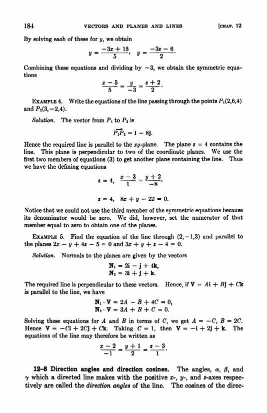
184 VECTORS AND PLANES AND LINES [CHAP. 12
By solving each of these for y, we obtain
-3z + 15 -32 - 6If--j
-> y- 2
--
Combining these equations and dividing by 3, we obtain the symmetric equa-
tions
x - 5_j/_
2 + 2
5 -32'EXAMPLE 4. Write the equations of the line passing through the points PI(2,6,4)
andP2(3,-2,4).
Solution. The vector from PI to P2 is
Hence the required line is parallel to the o#-plane. The plane 2 = 4 contains the
line. This plane is perpendicular to two of the coordinate planes. We use the
first two members of equations (3) to get another plane containing the line. Thus
we have the defining equations
,
-__2 = 4, Sx + y
- 22 = 0.
Notice that we could not use the third member of the symmetric equations because
its denominator would be zero. We did, however, set the numerator of that
member equal to zero to obtain one of the planes.
EXAMPLE 5. Find the equation of the line through (2, 1,3) and parallel to
the planes 2j y + 42 5 = and 3x + y + z 4 = 0.
Solution. Normals to the planes are given by the vectors
Hi = 2i - j + 4k,
N2= 3i + j + k.
The required line is perpendicular to these vectors. Hence, if V = Ai + Bj + Ckis parallel to the line, we have
Ni V = 2A - B + 4C =0,
N2 V = 3A + B + C = 0.
Solving these equations for A and B in terms of C, we get A = C, B = 2C.
Hence V = -Ci + 2Cj + Ck. Taking C =1, then V = -i + 2j + k. The
equations of the line may therefore be written as
x- 2_^ y + 1 2-3
-1 2 1
12-8 Direction angles and direction cosines. The angles, a, 0, and
7 which a directed line makes with the positive x-, y-, and 2-axes respec-
tively are called the direction angles of the line. The cosines of the direc-
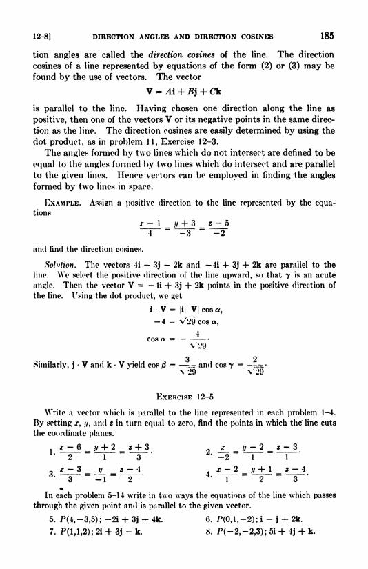
12-8] DIRECTION ANGLES AND DIRECTION COSINES 185
tion angles are called the direction cosines of the line. The direction
cosines of a line represented by equations of the form (2) or (3) may be
found by the use of vectors. The vector
V = A\ + Bj + Ck
is parallel to the line. Having chosen one direction along the line as
positive, then one of the vectors V or its negative points in the same direc-
tion as the line. The direction cosines are easily determined by using the
dot product, as in problem 11, Exercise 12-3.
The angles formed by two lines which do not intersect are defined to be
equal to the angles formed by two lines which do intersect and are parallel
to the given lines. Hence vectors can be employed in finding the angles
formed by two lines in space.
EXAMPLE. Assign a positive direction to the line represented by the equa-
tions
j - 1 // + 3 _ z - 5
4~
-3~
-2
and find the direction cosines.
Solution. The vectors 4i 3j 2k and 4i + 3j + 2k are parallel to the
line. We select the positive direction of the line upward, so that y is an acute
angle. Then the vector V = 4i -f 3j + 2k points in the positive direction of
the line. Using the dot product, we get
i. V =|i| |V|cosa,
4 = VlQcosa,4
COS Of = =V29
3 2Similarlv, j V and k V vield cos 3 = and cos y = -^=-
\ 29 \ 29
EXERCISE 12-5
Write a vector which is parallel to the line represented in each problem 1-4.
By setting j, //, and z in turn equal to zero, find the points in which the' line cuts
the coordinate planes.
. x - 6 i/ + 2 z + 3 i y -2 _ z - 3*
-** ~~ ~
3* ** y * ** A & 2r\
s=*~
*** *3-12 123
In each problem 5-14 write in two ways the equations of the line which passes
through the given point anil is parallel to the given vector.
5. P(4,-3,5); -2i + 3j + 4k. 6. P(0,l f -2); i-
J + 2k.
7. P(l,l,2); 2i + 3j- k. 8. P(-2,-2,3); 5i + 4j + k.
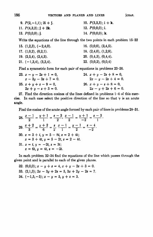
186 VECTORS AND PLANES AND LINES [CHAP.
9. P(2,-l,l); 2i + j. 10. P(3,3,3); i + k.
11. P(4,3,2);j + 2k. 12. P(0,0,0);i.
13. P(0,0,0);j. 14. P(0,0,0);k.
Write the equations of the line through the two points in each problem 15-22
15. (1,2,3), (-2,4,0). 16. (0,0,0), (3,4,5).
17. (1,0,2), (0,2,1). 18. (2,4,0), (1,2,8).
19. (2,5,4), (2,4,3). 20. (0,4,3), (0,4,4).
21. (-1,3,4), (3,3,4). 22. (0,0,2), (0,0,4)
Find a symmetric form for each pair of equations in problems 23-26.
23. x - y- 2* + 1 =
0, 24. x + y- 2* + 8 =
0,
x - Sy- 3* + 7 = 0. 2x - y
- 2z + 4 = 0.
25. x + y + z - 9 =0, 26. x + y
- z + 8 =0,
2x + y- i + 3 = 0. 2x - y + 2z + 6 = 0.
27. Find the direction cosines of the lines defined in problems 1-4 of this exer-
cise. In each case select the positive direction of the line so that y is an acute
angle.
Find the cosine of the acute angle formed by each pair of lines in problems 28-31 .
x ~ 1 V + * g -3 x - 1 y+ 1 z -39ft
1 2'
2 -2 1
+ 2 _ z x- 1 _ y-
1 _ z - 4
6~~
2' "1 ~T~"
-2'
30. x = 3 + *, y = 5 - 8*, z = 2 + 4J;
2 3 + 4t, y = 5 - 2*f* = 2 - 4*.
31. x =J, y = -2J, 2 = 3J;
x =6*, i/
=4*, 2 = -2t.
In each problem 32-34 find the equations of the line which pusses through the
given point and is parallel to each of the given planes.
32. (0,0,0); * -y + z = 4,x + y-2z + 3 = Q.
33. (2,1,3); 2x - 3y + 2z - 5, 3* + 2y- 2* = 7.
34. (-l,5,-5);z-</ =5,2/ + 2 = 3.
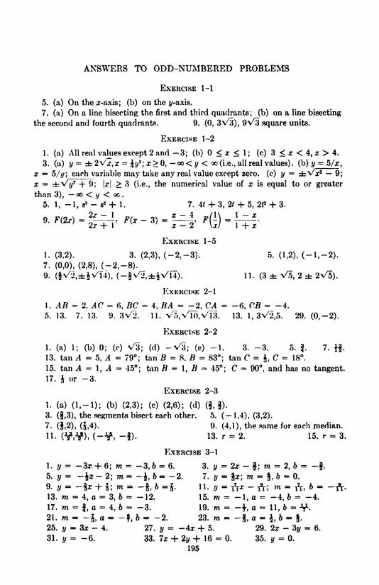
ANSWERS TO ODD-NUMBERED PROBLEMS
EXERCISE 1-1
5. (a) On the x-axis; (b) on the z/-axis.
7. (a) On a line bisecting the first and third quadrants; (b) on a line bisecting
the second and fourth quadrants. 9. (0, 3\/3), 9^3 square units.
EXERCISE 1-2
1 . (a) All real values except 2 and -3; (b) < x < 1; (c) 3 < x < 4, x > 4.
3. (a) y = 2\/j, z = J*/2
;z > 0,
- oo < ?/ < oo (i.e., all real values), (b) y = 5/x,
x =5///; each variable may take any real value except zero, (c) y dbVs2
9;
x = rtVj/2-f 9; |x| > 3 (i.e., the numerical value of x is equal to or greater
than 3), oo < jy < oc.
5. 1, -1," - s2 + 1. 7. 4< + 3, 2* + 5, 2t2 + 3.
EXERCISE 1-5
1. (3,2). 3. (2,3), (-2,-3). 5. (1,2), (-1.-2).7. (0,0), (2,8), (-2,-8)._9. (fv^iiv'H), (-f\/2,dbiVi4). 11. (3 V5, 2
EXERCISE 2-1
1. AB = 2,AC =fi, #C = 4, BA = -2, CA = -6, C = -4.
5. 13. 7. 13. 9. 3v/2. 11. VrtXlO.VlS. 13. 1, 3%/2,5. 29. (0,~2).
EXERCISE 2-2
1. (a) 1; (b) 0; (c) v/3; (d) -V3; (e) -1. 3. -3. 5. J. 7. .
13. tan ^1 = 5, A = 79; tan B = 8. # = 83; tan C =J, C = 18.
15. tan ^ =1, A = 45; tan B =
1, B = 45; C - 90, and has no tangent.
17. i or -3.
EXERCISE 2-3
1. (a) (1,-1); (b) (2,3); (c) (2,6); (d) (if).3. (f,3), the segments bisect each other. 5. (-1,4), (3,2).
7. (,2), (J,4). 9. (4,1), the same for each median.
H. (,), (-, -I). 13. r = 2. 15. r = 3.
EXERCISE 3-1
1. y = -3s -f 6; m = -3, 6 = 6. 3. y = 2x - f ;m =
2, 6 = -f .
5. ?/= -i* - 2; m = -i, 6 = -2. 7. y = Jx; m -
$, 6 - 0.
9. y - -fx + J; m = -f, 6 =J. 11. y = T\x - A; m --ft, 6 = -ft-
13. m =4, a = 3, 6 = -12. 15. m - -1, a = -4, 6 = -4.
17. m -f, a = 4, 6 - -3. 19. m = -|, a = 11, 6 = Y.
21. m - -J, a = -f 6 = -2. 23. m - -f, a =4, 6 = .
25. T/= 3x - 4. 27. y = -4x -f 5. 29. 2* - 3y = 6.
31. ?/= -6. 33. 7x + 2y + 16 = 0. 35. y = 0.
195

196 ANSWERS TO ODD-NUMBERED PROBLEMS
EXERCISE 3-1 cont'd.
37. 2x + 30 = 6. 39. 3z - 40 = 12. 41. x + y + 2 = 0.
43. 3z + 40 = 2. 45. 21z + 220 = 77. 47. 33* + 40 + 22 = 0.
49. 2s - y - 5. 51. 2z - 30 + 4 = 0. 53. z + 20 + 15 = 0.
55. y = 3. 57. Sx + 30 0. 59. 6x + + 37 = 0.
61. 6z + 70 = 11. 63. 2z + y- 2 = 0. 65. x = 3.
67. 8* - 270 = 58. 69. x = 0. 71. 2x - y + 1 - 0.
75. 2x - 30 =5, 3z + 20 = 14. 77. Ix + 50
- 41 =0, 5z - 70 + 13 = 0.
79. Sx - y- 19 = 0, x + Sy + 22 = 0. 81. y = 1, x = - 1.
83. 9z + y - 63 =0, x - 90
- 7 = 0.
85. (a) x - 4y - 1 = 0, 3z - y = 3, 2x + Zy = 24.
(b) 4* - 5y = 4, x + 7y = 23, 5x + 2y = 27; (tf , f).
(c) 3x - 2t/-
3, x + 3y = 15, 4x + y - 18; (ff , ).
(d) 4* + y-21,* + 3y- 11, 3x - 2y - 10; (ff, )
EXERCISE 3-2
1. . 3. 3\/2. 5. -^^- 7. 3.
9. 5. 11. 7x - 4?/= D. 13. a + 2y = 2fe. 15. 4x - ay = 4a.
17. x - 20 + 7 + k(bx - 7y-
3) = 0. 19. All pass through (0,4).
21. All have the slope-
. 23. All pass through (0,3).
25. All pass through the point of intersection of 4x 7y 7 = and y = 0.
27. The equations in order, omitting problems 22 and 25, are: 4x + 3// 12 = 0,
y = 2x - 6, 9s + 2y = 27, x -f y = 3, 7x + 3z/= 21, 3x + 820 - 9 = 0. No
line of the family of problem 22 or of problem 25 passes through (3,0). Why?29. 9x - 320 + 19 = 0. 31. 34x - 55 = 0. 33. 24x -f 240 -f 5 = 0.
35. 20x + 250 + 62 0, 7* - 70- 16 =
0, 27x + 180 -f 46 = 0.
37. x - =5, 3x + 30 + 1 = 0.
EXERCISE 4-1
1. 3z' + 20' - 0. 3. /2 - 6*'.
5. z/2 + 0'2 = 4. 7. z'0'
= 11.
9. (1,2), x/2 + 0" - 9. 11. (3,2), z'0'= 14.
13. (-3, -1), z" + 20/2 - 9. 15. (1,3), 0'
2 + 4z' - 0.
17. (-2, -2), 0'
2 + 10z' - 0.
EXERCISE 4-2
1. 0' + 2 = 0. 3. z'2 - 0'2 = 8. 5. 3z'2 + 0'
2 = 2.
7. /2 -4z' = 0. 9.45. 11. 22i.
EXERCISE 4-3
I. 3z' - 40' = 0. 3. S = arc tan J, 50' + 6 - 0.
5. 6 = 45, 0'2 -
40'- 4z' - 4 = 0. Then a translation yields 0"
2 - 4z" 0.
7. 6 = arc tan f, z/a + 40'2 + 4z' - 160' + 16 = 0. Then a translation gives
z"2 + 40"2 = 4.
II. (x + 3)2 =
0, two coincident lines.
13. (z + i-
iV3t)(z + \ + 4\/3i*)=
0, no graph.

ANSWERS TO ODD-NUMBERED PROBLEMS 197
EXERCISE 5-1
1. F(l,0); ends of latus rectum (l,-2), (1,2); directrix x = -1.
3. F(0,-f); ends of latus rectum (-5,-f), (5,-f); directrix y =f.
5. F(~f,0); ends of latus rectum ( f, f), ( i,f); directrix 4z = 3.
7. t/2 = 12*. 9. z/
2 = 24x. 11. x* = -I2y.
13. 3*2 + 16z/- 0. 15. y = -a:. 17. **
EXERCISE 5-2
1. F(0,4);3. F(d=5,0); r(13,0); B(0,12); (-5,
5. F(2V6,0); V(7,0); B(0,5);7. F(0,V2l); r(O f 5);B(2,0);9. F(0,
- = -7'54
+30
ly '
100^75' Z1
'3fl^9
23- ?7 + T? = ' 25 - 91 -4 an(i 94 -6 million miles.M 16
F^XERCISE 5-3
1. r(4,0); F(5,0); ?;
_|. 0,
|+
|0.
3. F(0,3); F(0. Vl3);|; |
-\=
0,|+
\= 0.
5. r(2,0); F(5.0); 21; |+ -^=
= 0,? -
-|=- 0.
7. r(0.6); FCO.i 6v7i2); 12; j + i/= 0, x - ;/
= 0.
** ?/'- i 11 tf T'
- 1 11x*
-(/t -1 l"i
*' - -v*-
19. jjj-9-1. "-21-4- 1 ' "'T'T- 1 - 15'T6 20
~ L
EXERCISE 5-4
1. (x-
2)1 + (y + 6)' - 25. 3. x> + (//
-4)' = 16.
5. (x-
4)s +(y + 3)'
= 25. 7. (y-
4)' = 12(j + 1).
9. (x + f)*=
4(t/-
2). 11. (y-3)5 = 12(z-
2). 13. x* =16(j/
-2).
15 '
(J~
5)'
+ (j/ 4)'
= L Center (5|4); F '
( '4) ' F(10 '4); F'
(2 '4) ' F(8 '4);
B'(5,0), B(5,8).
17.(yt 3)t + (g
"^4)
'
= L Center (4, -3); F'(4,-3-V3), F(4 >
O ^
F'(4,-4), F(4,-2); B'(4- V2.-3), B(4 + V2.-3).
19(?/-
1)' + (x-
5)' m j 21(x + 1)' + (y + 1)' = L
9 4 io y
23.(z~
3)> -f= I- <?(3,0); V'(-l,0), V(7,0); F'(-2,0), F(8,0).

198 ANSWERS TO ODD-NUMBERED PROBLEMS
EXERCISE 5-4 cont'd.
(y-
3)2_ (s
-3)
2
_ (y 2)2_
|-- 1. 29.
? g- 1.
37. Ellipse. 39. Hyperbola. 41. Hyperbola. 43. Parabola.
45. x =t/ 1, x = 2y. Hence the graph is two intersecting lines.
49. The greatest value is Vk
EXERCISE 6-1
1.0. 3. -5. 5. 4x3. 7. 2.
9. 3s2. 11. 6* -4. 13. -tor1
. 15. -I/a;2
.
17. -12ar8 + lOar3. 19. -4/x6
.
21. A# = 2z; 2x - y = 1. 23. Dty = -1/z2;x + y + 2 - 0.
25. Dxy = 2x - 4; y = -4. 27. A,i/ = 4s3 -8z; 16* - y = 32.
29. Dxy = -4x-6 + 4x'; y = 2.
EXERCISE 6-2
I. (0,2), maximum point. The slope is positive when x < and negative when
x > 0.
3. (2, -4) minimum point. The slope is negative when x < 2 and positive
when x > 2.
5. (3,10), maximum point. The slope is positive when x < 3 and negative
when x > 3.
7. (0,0), neither a maximum nor a minimum point. The slope is negative at
all points except the origin.
9. The slope is zero at (1,J) and is positive at all other points.
II. ( 1,1), maximum point; (0,0), minimum point. The slope is positive when
x < 1 and when x > 0. The slope is negative when 1 < x < 0.
13. (0,4), maximum point; (2,0), minimum point. The slope is positive when
x < and when x > 2. The slope is negative when < x < 2.
15. (0,0), (1,-1). 17. (0,1), (1,-B).
19. (0,1), (I,*), (2,1). 21. (-1.A), (!,-).
EXERCISE 6-3
1. A square 100 yds. on a side. 3. 2000 sq. yd.
5 10 - 2V7 = l 57.
n^ approximatelyt 7> 6
/
by 6'
by 3'.o
250 0009. Radius 2 in., height 4 in. 11. <~ cu. in.
EXERCISE 7-1
1. Period ir, amplitude 1. 3. Period 6^r, amplitude 1.
5. Period ITT. 7. Period TT. 9. Period JTT. il. Period 4, amplitude 2.
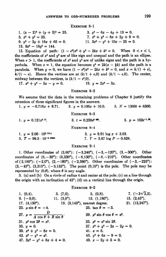
ANSWERS TO ODD-NUMBERED PROBLEMS 199
EXERCISE 8-1
1. (x-
2)2 + (y + 3)
2 = 25. 3. y2 - 6x - 4y + 13 = 0.
5. x2 + i/2 = 25. 7. x2 + i/'
- 8x + 2?/ + 9 = 0.
9. i/2 - 2y + 16x + 65 = 0. 11. 3x2 -
y2 + lOx - 25 = 0.
13. 9*' - 16y2 = 144.
15. Equation of path: (1- e2)x
2 + t/2 - 2kx + A;
2 = 0. When < e < 1,
the coefficients of x2 and y1 are of like sign and unequal and the path is an ellipse.
When e > 1, the coefficients of x1 and y1 are of unlike signs and the path is a hy-
perbola. When e = 1, the equation becomes y1 = 2k(x Jfc) and the path is a
parabola. When y =0, we have (1
- e2)x2 - 2kx + fc
2 =0, and x = Jb/(l + e),
k/ (1 e). Hence the vertices are at (fc/1 + e,0) and (&/1 e,0). The center,
midway between the vertices, is (k/\ e2,0).
17. x2 + i/2 - 5x - t/
= 0. 19. t/= 2x2 - 3x.
EXERCISE 8-2
We assume that the data in the remaining problems of Chapter 8 justify the
retention of three significant figures in the answers.
1. y = -0.718x + 8.71. 3. y = O.lOOx + 10.0. 5. AT = 1380* + 6300.
EXERCISE 8-3
1. y = 0.121x3 3. t = 0.259s0488 . 5. p = lOSir 1-*.
EXERCISE 8-4
1. y = 2.00 10 - l 3. y = 9.91 log x + 3.03.
5. T = 99.5 - 10- o98" 7. V = 3.87 log P - 0.828.
EXERCISE 9-1
1. Other coordinates of (3,60): (-3,240), (-3, -120), (3, -300). Other
coordinates of (6, -30): (6,330), (-6,150), (-6, -210). Other coordinates
of (2,180): (-2,0), (2, -180), (-2,360). Other coordinates of (-3, -225):
(3, -45), (3,315), (-3,135). The point (0,10) is the pole. The pole may be
represented by (0,0), where B is any angle.
3. (a) and (b) On a circle of radius 4 and center at the pole; (c) on a line through
the origin with an inclination of 45; (d) on a vertical line through the origin.
EXERCISE 9-2
1. (0,4). 3. (7,0). 5. (0,8). 7. (-3^3,3).9. C-9,0). 11. (3,0). 13. (1,180). 15. (2,45).
17. (4,150). 19. (5,143), nearest degree. 21. (13,247).
23. p sin B = -4. 25. tan B = -3.
27. p -: Q , p . v 29. p2 sin B cos B = a2
.* A cos B + B sin B*
31. p2 cos 26 = a2
. 33. p2 = a2 sin 26.
35. y = 0. 37. x2 + ?/
2 - 2x - 2y = 0.
39. x2 + if- 8x = 0. 41. x = 6.
43. x2 -y2 - a2
. 45. y2 + 6x - 9 - 0.
47. 3x2 -2/2 + 8x + 4 = 0. 49. x - 2y + 5 = 0.

200 ANSWERS TO ODD-NUMBERED PROBLEMS
EXERCISE 9-4
7. Center (4,0), radius 4. 9. Center (5,270), radius 5.
11. (a) p2 - 8p cos e + 12 - 0; (b) p
2 - 8p sin + 12 = 0;
(c) p - 4 cos - 0.
EXERCISE 9-6
I. (1,60), (1,300). 3. (3^2,45), (3^2,315).
5. (a,90), (a,270). 7. (2,0). 9. (f,60), (|,300).
II. (1,0), (-$,233). Arc sin (-f) 233, to the nearest degree.
13. (1,60). 15. (1,60), (1,300).
17. (3,180). 19. (2,60), (2,300), (-1,180).
EXERCISE 10-1
1. 3x + y = 6. 3. xy = 6. 5. *2 + 9^ = 9.
7. 9*' + 16z/2 - 144. 9. x2 + y
2 - 2x. 11. x* + 4</= 4.
13. x2 -i/2 = 1. 15 z2 + zt/
- 1 - 0.
17. 2x2 -2xy + y*
= 1. 19. ?/2 - *2 - 4.
EXERCISE 10-2
1. x = 40 V2<, y = 40 \/2/ - 16J2;x* - 200x + 200z/ = 0, The greatest height
is 50 feet, and the ball strikes the ground 100 feet away.ax1
3. x = Vot, y = J0/2
; y = %r-2- In 2 seconds the projectile falls 60 feet and
travels 2v* feet horizontally.
EXERCISE 12-1
1. 11. 3. V102.
5. AB - -6i - 6j, BC = -6j - 6k, CA = 6i + 12j + 6k. The lengths are
6\/2, 6\/2, 6\/6.
7. AB - i + 2j + 2k, 5C - -3i - 3j, (M - 2i + j- 2k, The lengths are
3, 3V2, 3.
6i + 3j- 6k 2i j
- 3kW. ~ -
- -1JL. =
9 VT413. 4i + fj, to the mid-point; 3i - j + 4k and 5i + j + k, to the trisection
points.
15. Center (-2,1, -3), radius Vl4. 17. i + 2j + 2k.
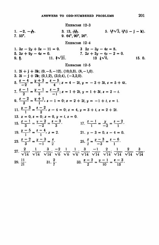
ANSWERS TO ODD-NUMBERED PROBLEMS 201
EXERCISE 12-3
1. -2, -*. 3. 13, tft. 5. tfV5, V(i - J-
k).
7. 55. 9. 64, 90, 26.
EXERCISE 12-4
1. 3x - 2y + 5 - 11 = 0. 3 2x - 3y - 4* = 8.
5. 3* + 9y- 40 - 0. 7. 2x + 3y
- 4* - 2 - 0.
9. f. 11. f\/2l. 13 *\/6. 15. 0.
EXERCISE 12-5
1. 2i + j + 3k; (O f -5,-12), (10,0,3), (8, -1,0).
3. 81 - J + 2k; (0,1,2), (3,0,4), (-3,2,0).
INDEX
Abscissa, 1
Addition of ordinates, 75, 105
Aids in graphing, 6, 130
Amplitude, 100
Analytic proofs, 28
Anglebetween two lines, 24
between two planes, 180
between two vectors, 176
vectorial, 120
Angles, direction, 184
Applications of conies, 74
Asymptotes, 13, 71
Axes
coordinate, 1, 151
of ellipse, 65
of hyperbola, 70
rotation of, 49
translation of, 45
x, y, and z in space, 151
Axis
of parabola, 59
polar, 120
Best-fitting line, 110
Cardioid, 131
Center, 65, 70
Circle
equations of, 64, 76, 127, 142
through three points, 108
involute of, 149
Cissoid of Diocles, 150
Components of a vector, 1 70
Cone
right circular, 56
elliptic, 165
Conies, 56
applications of, 75
degenerate, 56, 58
identification of, 79
in polar coordinates, 128
simplified equations of, 53, 57
standard forms of equations of, 75,
Conic section, 56
Conjugate axis, 70
Constant, 3
Constant e} the, 103
Coordinates
polar, 120
polar to rectangular, 122
rectangular, 1
rectangular to polar, 121
space, 151
Cosines, direction, 184
Curve fitting, 109
Curves
exponential, 103
inverse trigonometric, 101
logarithmic, 104
trigonometric, 98
Cycloid, 147
curtate, 148
prolate, 148
Cylinder, 153
Cylindrical surface, 1 53
Decreasing function, 89
Degenerate conic, 56, 58
Dependent variable, 4
Derivatives, 85
formulas for, 86
used in graphing, 89
Descartes, 1
Directed line, 17
Directed line segment, 17
Direction angles, 184
Direction cosines, 184
Directrix of a parabola, 60
Distance
between two points, 18, 19
from a line to a point, 37, 38
from a plane to a point, 179, 181
Double-valued, 4
Dot product, 174
Eccentricity, 68, 73
76 Element of a cylinder, 154
202
INDEX 203
Ellipse, 64-68
in polar coordinates, 128
parametric equations of, 142
Ellipsoid, 159
Elliptic cone, 165
Elliptic paraboloid, 163
Empirical equation, 109
Equation
empirical, 109
of a given curve, 107
graph of, 5, 124
locus of, 5, 152
Equation of the first degree
general form of, 31
intercept form of, 33
normal form of, 39
point-slope form of, 33
slope-intercept form of, 32
in three variables, 155
two-point form of, 33
Equation of second degree
general form of, 52, 56
simplified forms of, 53, 57
standard forms of, 75, 76
in three variables, 156
Equations of a line, 181
in polar coordinates. 126, 127
Equilateral hyperbola, 73
Excluded values, 133
Exponential curve, 103
Exponential equation, 103
Exponential formula, 117
Extent of graph, 8
Extreme value, 100
Family of lines, 40
through intersection of two lines, 41
Foci
of ellipse, 65
of hyperbola, 70
Focus of a parabola, 60
Focus-directrix property, 59, 128
Four-leaved rose, 133
Function, 3
decreasing, 89
increasing, 89
periodic, 98
transcendental, 98
General linear equation, 31, 155
Graph, 5
extent of, 8
of equation in factored form, 10
of parametric equations, 143
of polar coordinate equations, 124
of sum of two functions, 75, 105
Graphing, aids in, 6, 130
Graphs, intersections of, 11, 138
Horizontal segment, 18
Hyperbola, 70-73
in polar coordinates, 128
Hyperbolic paraboloid, 164
Hyperboloidof one sheet, 160
of two sheets, 161
Hypocycloid of four cusps, 150
Identification of a conic, 79
Inclination of a line, 21
Increasing function, 89
Independent variable, 4
Intercept form of equation, 33
Intercepts, 6
Intersections of graphs, 11, 138
Invariant, 80
Inverse trigonometric functions, 101
Involute of a circle, 149
Latus rectum, 60, 67, 70
Least squares, method of, 110
Lemniscate, 135
Limagon, 134
Line
best-fitting, 110
directed, 17
inclination of, 21
slope of, 21
Linear equation, 11, 155
Line segmentformula for length, 18, 19
formulas for division of, 28
formulas for mid-point, 27
Locus of an equation, 5, 31, 152
Logarithm, definition of, 104
Logarithmic curve, 104
Logarithmic formula, 117

204 INDEX
Logarithmic paper, 114
Logarithmic spiral, 136
Major axis, 65
Maximum of a function, 92
Maximum point, 92
Method of least squares, 1 10
Mid-point formulas, 27
Minimum of a function, 92
Minimum point, 92
Minor axis, 65
Nonlinear fits, 113
Octant, 151
Ordinate, 1
Ordinates, addition of, 78, 105
Origin, 1, 120
Parabola, 58-63
in polar coordinates, 128
Parameter, 40, 141
Parametric equations, 141
of a circle, 142
of a cycloid, 147
of an ellipse, 142
of a line, 182
of p?th of a projectile, 146
Path of a projectile, 146
Period of a function, 98
Periodic function, 98
Plane, equation of, 178
Point-slope form, 33
Polar axis, 120
Polar coordinates, 120
of conies, 128
of lines, 126, 127
to rectangular coordinates, 122
Pole, 120
Power formula, 114
Projectile, path of, 146
Projecting plane, 180
Prolate cycloid, 148
Proofs, analytic, 28
Quadrant, 1
Quadric surface, 156, 157
Radius vector, 120
Range, 4
Reciprocal spiral, 136
Rectangular coordinates, 1
to polar coordinates, 121
Rectangular hyperbola, 73
Residual of a point, 110
Rose curves, 133
Rotation of axes, 49
Scalar, 167
product, 174
projection, 175
Second degree equation, 52, 156
Semilogarithmic paper, 117
Simplified equations of conies, 51, 53,
57
Single-valued, 4
Slant segment, 18
Slope
of a curve, 84
of a line, 21
formula for, 23
Slope-intercept form, 32
Space coordinates, 151
Spirals, 136
Standard forms of equations, 75, 76
Surface
cylindrical, 154
quadric, 156
of revolution, 160
Symmetric equations of a line, 182
Symmetry, 7
tests for, 8, 132
System of lines, 41
Tangent to a curve, 84
Tangent lines at the origin, 131
Traces, 155
Transcendental functions, 98
Transformation of coordinates, 45
Translation of axes, 45
Transverse axis, 70
Trigonometric curves, 98
Two-point form, 33
Unit vector, 170
INDEX 205
Variable, 3 Vectors (cont'd)
dependent, 4 in space, 172
independent, 4 projection of, 175
Vectorial angle, 121 scalar product of two, 174
Vectors, 167 sum of, 168
components of, 170, 172 Vertex, 59, 65, 70
difference of, 168 Vertical segment, 18
direction of, 167
magnitude of, 167 Witch of Agnesi, 149
in a plane, 169


