
Amol Deshpande, University of Maryland
Zachary G. Ives, University of Pennsylvania
Vijayshankar Raman, IBM Almaden Research Center
Thanks to Joseph M. Hellerstein, University of California, Berkeley
Adaptive Query Processing
Query Processing: Adapting to the World
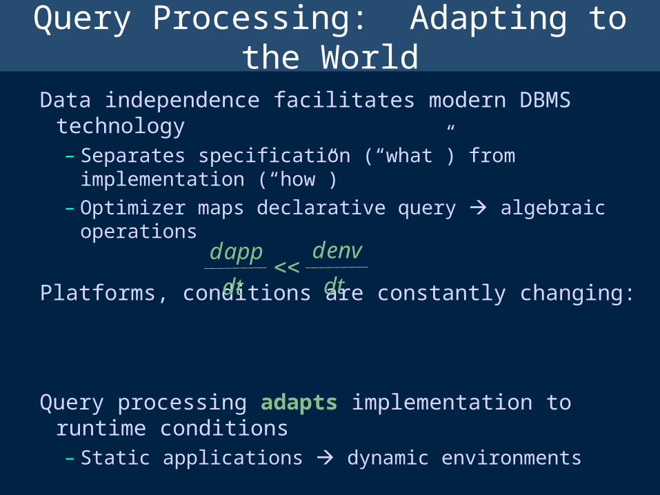
Data independence facilitates modern DBMS technology– Separates specification (“what”) from implementation (“how”)
– Optimizer maps declarative query algebraic operations
Platforms, conditions are constantly changing:
Query processing adapts implementation to runtime conditions– Static applications dynamic environments
d app
dt
d env
dt

Dynamic Programming + Pruning Heuristics
Query Optimization and Processing(As Established in System R [SAC+’79])
> UPDATE STATISTICS ❚
cardinalitiesindex lo/hi key
> SELECT * FROM Professor P, Course C, Student S WHERE P.pid = C.pid AND S.sid = C.sid❚
Professor Course Student

Traditional Optimization Is Breaking
In traditional settings:– Queries over many tables
– Unreliability of traditional cost estimation
– Success & maturity make problems more apparent, critical
In new environments:– e.g. data integration, web services, streams, P2P, sensor nets, hosting
– Unknown and dynamic characteristics for data and runtime
– Increasingly aggressive sharing of resources and computation
– Interactivity in query processing
Note two distinct themes lead to the same conclusion:– Unknowns: even static properties often unknown in new environments
and often unknowable a priori
– Dynamics: can be very high
Motivates intra-query adaptivity
denvdt

A Call for Greater Adaptivity
System R adapted query processing as stats were updated– Measurement/analysis: periodic
– Planning/actuation: once per query
– Improved thru the late 90s (see [Graefe ’93] [Chaudhuri ’98])
Better measurement, models, search strategies
INGRES adapted execution many times per query– Each tuple could join with relations in a different order
– Different plan space, overheads, frequency of adaptivity
Didn’t match applications & performance at that time
Recent work considers adaptivity in new contexts

Observations on 20thC Systems
Both INGRES & System R used adaptive query processing– To achieve data independence
They “adapt” at different timescales– Ingres goes ‘round the whole loop many times per query
– System R decouples parts of loop, and is coarser-grained
• measurement/modeling: periodic
• planning/actuation: once per query
Query Post-Mortem reveals different relational plan spaces– System R is direct: each query mapped to a single relational algebra stmt
– Ingres’ decision space generates a union of plans over horizontal partitions
• this “super-plan” not materialized -- recomputed via FindMin
Both have zero-overhead actuation– Never waste query processing work

Tangentially Related Work
An incomplete list!!!
Competitive Optimization [Antoshenkov93]
– Choose multiple plans, run in parallel for a time, let the most promising finish
• 1x feedback: execution doesn’t affect planning after the competition Parametric Query Optimization [INSS92, CG94, etc.]
– Given partial stats in advance. Do some planning and prune the space. At runtime, given the rest of statistics, quickly finish planning.
• Changes interaction of Measure/Model and Planning
• No feedback whatsoever, so nothing to adapt to! “Self-Tuning”/“Autonomic” Optimizers [CR94, CN97, BC02, etc.]
– Measure query execution (e.g. cardinalities, etc.)
• Enhances measurement, on its own doesn’t change the loop
– Consider building non-existent physical access paths (e.g. indexes, partitions)
• In some senses a separate loop – adaptive database design
• Longer timescales

Tangentially Related Work II
Robust Query Optimization [CHG02, MRS+04, BC05, etc.]
– Goals: • Pick plans that remain predictable across wide ranges of scenarios• Pick least expected cost plan
– Changes cost function for planning, not necessarily the loop.• If such functions are used in adaptive schemes, less fluctuation [MRS+04]
– Hence fewer adaptations, less adaptation overhead
Adaptive query operators [NKT88, KNT89, PCL93a, PCL93b]
– E.g. memory-adaptive sort and hash-join– Doesn’t address whole-query optimization problems– However, if used with AQP, can result in complex feedback loops
• Especially if their actions affect each other’s models!

Extended Topics in Adaptive QP
An incomplete list!!
Parallelism & Distribution– River [A-D03]
– FLuX [SHCF03, SHB04]
– Distributed eddies [TD03]
Data Streams– Adaptive load shedding
– Shared query processing
Tutorial Focus
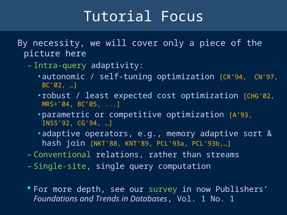
By necessity, we will cover only a piece of the picture here– Intra-query adaptivity:
• autonomic / self-tuning optimization [CR’94, CN’97, BC’02, …]
• robust / least expected cost optimization [CHG’02, MRS+’04, BC’05, ...]
• parametric or competitive optimization [A’93, INSS’92, CG’94, …]
• adaptive operators, e.g., memory adaptive sort & hash join [NKT’88, KNT’89, PCL’93a, PCL’93b,…]
– Conventional relations, rather than streams
– Single-site, single query computation
For more depth, see our survey in now Publishers’ Foundations and Trends in Databases, Vol. 1 No. 1

Tutorial Outline
Motivation
Non-pipelined execution
Pipelined execution
– Selection ordering
– Multi-way join queries
Putting it all in context
Recap/open problems

Low-Overhead Adaptivity: Non-pipelined Execution

Late Binding; Staged Execution
Materialization points make natural decision points where the next stage can be changed with little cost:
– Re-run optimizer at each point to get the next stage– Choose among precomputed set of plans – parametric query
optimization [INSS’92, CG’94, …]
AR
NLJ
sort
C
B
MJ
MJ
sort
Normal execution: pipelines separated by materialization points
e.g., at a sort, GROUP BY, etc.
materialization point

Mid-query Reoptimization[KD’98,MRS+04]
Choose checkpoints at which to monitor cardinalitiesBalance overhead and opportunities for switching plans
If actual cardinality is too different from estimated,Avoid unnecessary plan re-optimization (where the plan doesn’t change)
Re-optimize to switch to a new planTry to maintain previous computation during plan switching
Most widely studied technique:-- Federated systems (InterViso 90, MOOD 96), Red Brick,
Query scrambling (96), Mid-query re-optimization (98), Progressive Optimization (04), Proactive Reoptimization (05), …
Where?
How?
When?
AR
NLJ
B
C
HJ
MJ
sort
C
B
MJ
MJ
sort
Challenges

Where to Place Checkpoints?
Lazy checkpoints: placed above materialization points – No work need be wasted if we switch plans here
Eager checkpoints: can be placed anywhere– May have to discard some partially computed results
– Useful where optimizer estimates have high uncertainty
A
C
B
R
MJ
NLJ
MJ
sort
More checkpoints more opportunities for switching plans
Overhead of (simple) monitoring is small [SLMK’01]
Consideration: it is easier to switch plans at some checkpoints than others
sort
Lazy
Eager
When to Re-optimize?
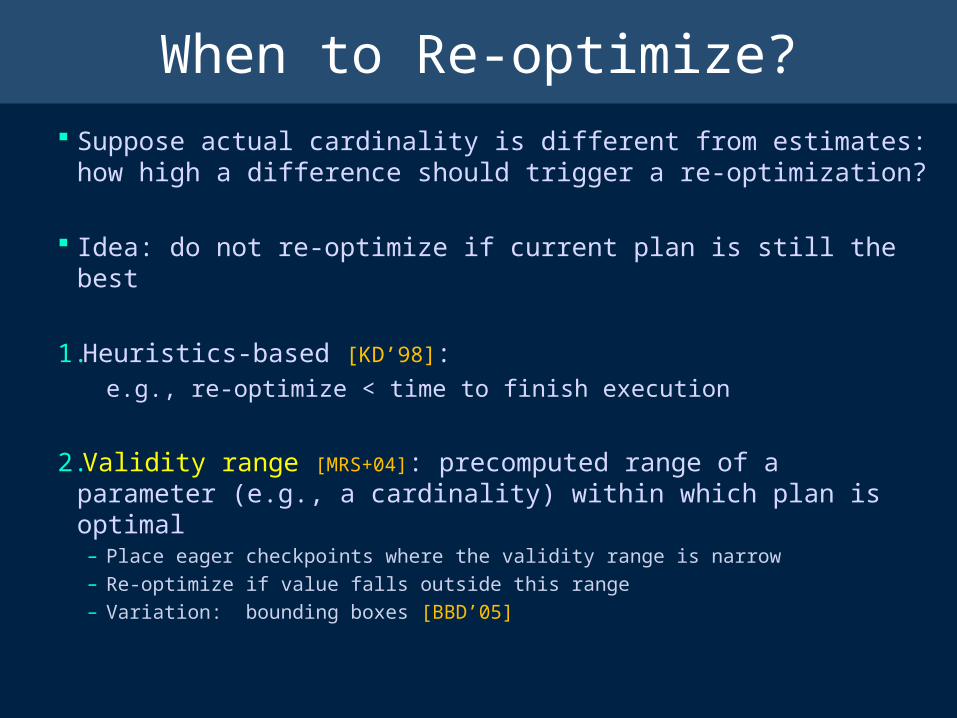
Suppose actual cardinality is different from estimates:how high a difference should trigger a re-optimization?
Idea: do not re-optimize if current plan is still the best
1.Heuristics-based [KD’98]:e.g., re-optimize < time to finish execution
2.Validity range [MRS+04]: precomputed range of a parameter (e.g., a cardinality) within which plan is optimal – Place eager checkpoints where the validity range is narrow
– Re-optimize if value falls outside this range
– Variation: bounding boxes [BBD’05]

How to Reoptimize
Getting a better plan:– Plug in actual cardinality information acquired during this
query (as possibly histograms), and re-run the optimizer
Reusing work when switching to the better plan:– Treat fully computed intermediate results as materialized
views• Everything that is under a materialization point
– Note: It is optional for the optimizer to use these in the new plan
Other approaches are possible (e.g., query scrambling [UFA’98])

Pipelined Execution

Adapting Pipelined Queries
Adapting pipelined execution is often necessary:– Too few materializations in today’s systems
– Long-running queries
– Wide-area data sources
– Potentially endless data streams
The tricky issues:– Some results may have been delivered to the user
• Ensuring correctness non-trivial
– Database operators build up state• Must reason about it during adaptation• May need to manipulate state
Adapting Pipelined Queries
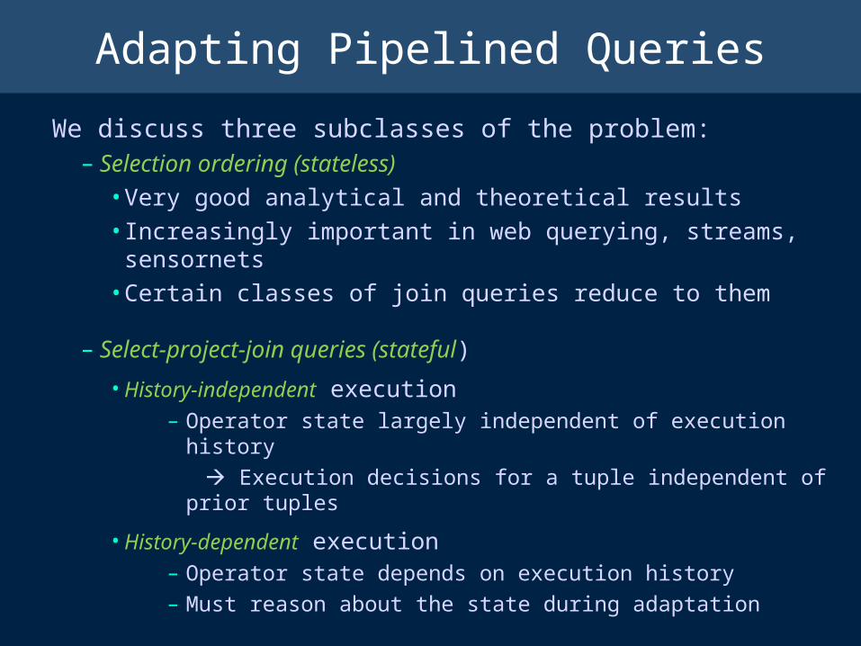
We discuss three subclasses of the problem:– Selection ordering (stateless)
• Very good analytical and theoretical results
• Increasingly important in web querying, streams, sensornets
• Certain classes of join queries reduce to them
– Select-project-join queries (stateful)
• History-independent execution– Operator state largely independent of execution history
Execution decisions for a tuple independent of prior tuples
• History-dependent execution– Operator state depends on execution history– Must reason about the state during adaptation

Pipelined Execution Part I:Adaptive Selection Ordering

Adaptive Selection Ordering
Complex predicates on single relations common– e.g., on an employee relation:
((salary > 120000) AND (status = 2)) OR
((salary between 90000 and 120000) AND (age < 30) AND (status = 1)) OR …
Selection ordering problem:
Decide the order in which to evaluate the individual predicates against the tuples
We focus on conjunctive predicates (containing only AND’s) Example Query
select * from Rwhere R.a = 10 and R.b < 20 and R.c like ‘%name%’;
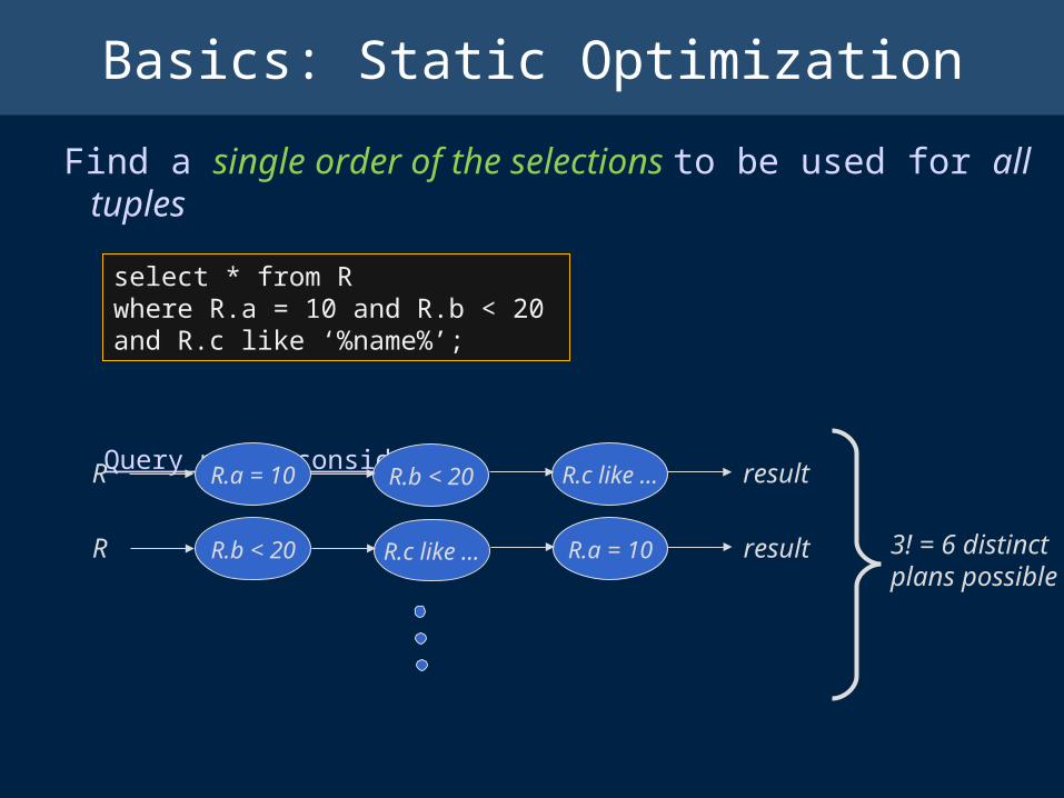
Basics: Static Optimization
Find a single order of the selections to be used for all tuples
Query
Query plans considered
R.a = 10 R.b < 20R resultR.c like …
R.b < 20 R.c like …R resultR.a = 10 3! = 6 distinctplans possible
select * from Rwhere R.a = 10 and R.b < 20 and R.c like ‘%name%’;

Static Optimization
Cost metric: CPU instructions
Computing the cost of a plan– Need to know the costs and the selectivities of the predicates
R.a = 10 R.b < 20R resultR.c like …
cost(plan) = |R| * (c1 + s1 * c2 + s1 * s2 * c3)
R1 R2 R3
costs c1 c2 c3selectivities s1 s2 s3
cost per c1 + s1 c2 + s1 s2 c3tuple
Independence assumption

Static Optimization
Rank ordering algorithm for independent selections [IK’84]– Apply the predicates in the decreasing order of rank:
(1 – s) / c
where s = selectivity, c = cost
For correlated selections:– NP-hard under several different formulations
• e.g. when given a random sample of the relation
– Greedy algorithm, shown to be 4-approximate [BMMNW’04]:
• Apply the selection with the highest (1 - s)/c
• Compute the selectivities of remaining selections over the result
– Conditional selectivities
• Repeat
Conditional Plans ? [DGHM’05]

Adaptive Greedy [BMMNW’04]
Context: Pipelined query plans over streaming data
Example:
R.a = 10 R.b < 20 R.c like …
Initial estimated selectivities
0.05 0.1 0.2
Costs 1 unit 1 unit 1 unit
Three independent predicates
R.a = 10 R.b < 20R resultR.c like …R1 R2 R3
Optimal execution plan orders by selectivities (because costs are identical)

Adaptive Greedy [BMMNW’04]
1. Monitor the selectivities over recent past (sliding window)
2. Re-optimize if the predicates not ordered by selectivities
R.a = 10 R.b < 20R resultR.c like …R1 R2 R3
Rsample
Randomly sample R.a = 10
R.b < 20
R.c like …
estimate selectivities of the predicatesover the tuples of the profile
ReoptimizerIF the current plan not optimal w.r.t. these new selectivitiesTHEN reoptimize using the Profile
Profile

Adaptive Greedy [BMMNW’04]
Correlated Selections– Must monitor conditional selectivities
monitor selectivities sel(R.a = 10), sel(R.b < 20), sel(R.c …)
monitor conditional selectivities sel(R.b < 20 | R.a = 10) sel(R.c like … | R.a = 10) sel(R.c like … | R.a = 10 and R.b < 20)
R.a = 10 R.b < 20R resultR.c like …R1 R2 R3
Rsample
Randomly sample R.a = 10
R.b < 20
R.c like …
(Profile)
ReoptimizerUses conditional selectivities to detect violationsUses the profile to reoptimize
O(n2) selectivities need to be monitored

Adaptive Greedy [BMMNW’04]
Advantages: – Can adapt very rapidly– Handles correlations– Theoretical guarantees on performance [MBMW’05]
Not known for any other AQP algorithms
Disadvantages:– May have high runtime overheads
• Profile maintenance– Must evaluate a (random) fraction of tuples against all
operators
• Detecting optimality violations• Reoptimization cost
– Can require multiple passes over the profile

Eddies [AH’00]
Query processing as routing of tuples through operators
Pipelined query execution using an eddy
An eddy operator• Intercepts tuples from sources and output tuples from operators• Executes query by routing source tuples through operators
A traditional pipelined query plan
R.a = 10 R.b < 20R resultR.c like …R1 R2 R3
EddyR
result
R.a = 10
R.c like …
R.b < 20
Encapsulates all aspects of adaptivity in a “standard”
dataflow operator: measure, model, plan and
actuate.

Eddies [AH’00]
a b c …
15 10 AnameA …
An R Tuple: r1
r1
r1
EddyR
result
R.a = 10
R.c like …
R.b < 20

ready bit i : 1 operator i can be applied 0 operator i can’t be applied
Eddies [AH’00]
a b c … ready done
15 10 AnameA … 111 000
An R Tuple: r1
r1
Operator 1
Operator 2
Operator 3
EddyR
result
R.a = 10
R.c like …
R.b < 20

done bit i : 1 operator i has been applied 0 operator i hasn’t been applied
Eddies [AH’00]
a b c … ready done
15 10 AnameA … 111 000
An R Tuple: r1
r1
Operator 1
Operator 2
Operator 3
EddyR
result
R.a = 10
R.c like …
R.b < 20

Eddies [AH’00]
a b c … ready done
15 10 AnameA … 111 000
An R Tuple: r1
r1
Operator 1
Operator 2
Operator 3
Used to decide validity and need of applying operators
EddyR
result
R.a = 10
R.c like …
R.b < 20

Eddies [AH’00]
a b c … ready done
15 10 AnameA … 111 000
An R Tuple: r1
r1
Operator 1
Operator 2
Operator 3
satisfiedr1
r1
a b c … ready done
15 10 AnameA … 101 010
r1
not satisfied
eddy looks at the next tuple
For a query with only selections, ready = complement(done)
EddyR
result
R.a = 10
R.c like …
R.b < 20

Eddies [AH’00]
a b c …
10 15 AnameA …
An R Tuple: r2
Operator 1
Operator 2
Operator 3
r2EddyR
result
R.a = 10
R.c like …
R.b < 20
satisfied
satisfied
satisfied

Eddies [AH’00]
a b c … ready done
10 15 AnameA … 000 111
An R Tuple: r2
Operator 1
Operator 2
Operator 3
r2
if done = 111, send to output
r2
EddyR
result
R.a = 10
R.c like …
R.b < 20
satisfied
satisfied
satisfied

Eddies [AH’00]
Adapting order is easy– Just change the operators to which tuples are sent
– Can be done on a per-tuple basis
– Can be done in the middle of tuple’s “pipeline”
How are the routing decisions made?
Using a routing policy
Operator 1
Operator 2
Operator 3
EddyR
result
R.a = 10
R.c like …
R.b < 20

Routing Policy 1: Non-adaptive
Simulating a single static order– E.g. operator 1, then operator 2, then operator 3
Routing policy: if done = 000 route to 1 100 route to 2 110 route to 3
table lookups very efficient
Operator 1
Operator 2
Operator 3
EddyR
result
R.a = 10
R.c like …
R.b < 20

Overhead of Routing
PostgreSQL implementation of eddies using bitset lookups [Telegraph Project] Queries with 3 selections, of varying cost
– Routing policy uses a single static order, i.e., no adaptation
0
0.2
0.4
0.6
0.8
1
1.2
1.4
0 μsec 10 μsec 100 μsec
Selection cost
No
rmali
zed
Co
st
No-eddies
Eddies
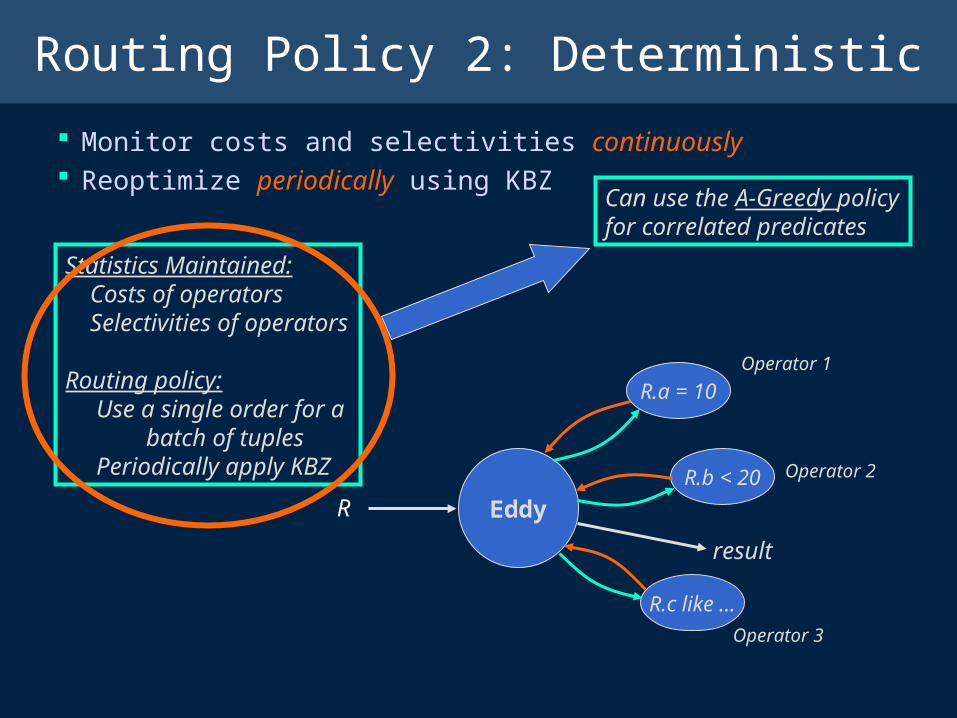
Routing Policy 2: Deterministic
Monitor costs and selectivities continuously Reoptimize periodically using KBZ
Statistics Maintained: Costs of operators Selectivities of operators
Routing policy: Use a single order for a batch of tuples Periodically apply KBZ
Operator 1
Operator 2
Operator 3
EddyR
result
R.a = 10
R.c like …
R.b < 20
Can use the A-Greedy policy for correlated predicates

Overhead of Routing and Reoptimization
Adaptation using batching– Reoptimized every X tuples using monitored selectivities
– Identical selectivities throughout experiment measures only the overhead
0
1
2
3
4
5
6
0 μsec 10 μsec 100 μsec
Selection Cost
No
rmal
ized
Co
st No-eddies
Eddies - No reoptimization
Eddies - Batch Size = 100 tuples
Eddies - Batch Size = 1 tuple
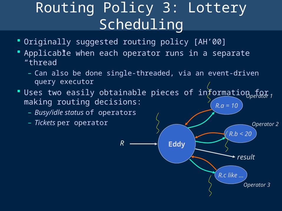
Routing Policy 3: Lottery Scheduling
Originally suggested routing policy [AH’00] Applicable when each operator runs in a separate “thread”
– Can also be done single-threaded, via an event-driven query executor
Uses two easily obtainable pieces of information for making routing decisions:– Busy/idle status of operators
– Tickets per operatorOperator 1
Operator 2
Operator 3
EddyR
result
R.a = 10
R.c like …
R.b < 20

Routing Policy 3: Lottery Scheduling
Routing decisions based on busy/idle status of operators
Rule: IF operator busy, THEN do not route more tuples to it
Rationale: Every thread gets equal time SO IF an operator is busy, THEN its cost is perhaps very high
Operator 1
Operator 2
Operator 3
EddyR
result
R.a = 10
R.c like …
R.b < 20
BUSY
IDLE
IDLE
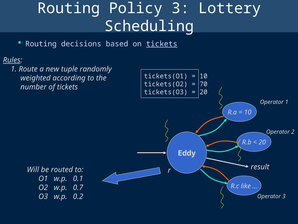
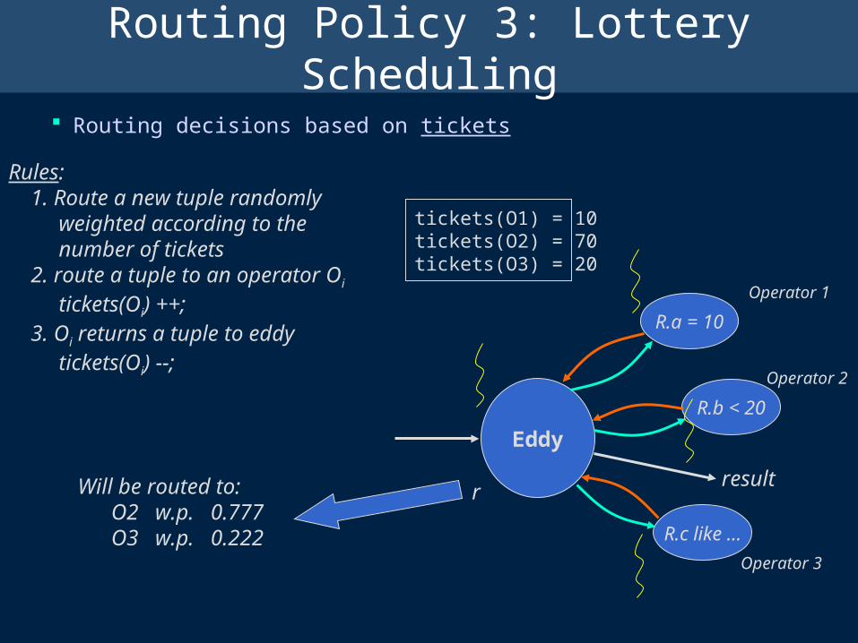
Routing Policy 3: Lottery Scheduling
Routing decisions based on tickets
Rules: 1. Route a new tuple randomly weighted according to the number of tickets
tickets(O1) = 10tickets(O2) = 70tickets(O3) = 20
Will be routed to: O1 w.p. 0.1 O2 w.p. 0.7 O3 w.p. 0.2
Operator 1
Operator 2
Operator 3
Eddy
result
R.a = 10
R.c like …
R.b < 20
r

Routing Policy 3: Lottery Scheduling
Routing decisions based on tickets
Rules: 1. Route a new tuple randomly weighted according to the number of tickets
tickets(O1) = 10tickets(O2) = 70tickets(O3) = 20
r
Operator 1
Operator 2
Operator 3
Eddy
result
R.a = 10
R.c like …
R.b < 20

Routing Policy 3: Lottery Scheduling
Routing decisions based on tickets
Rules: 1. Route a new tuple randomly weighted according to the number of tickets 2. route a tuple to an operator Oi
tickets(Oi) ++;Operator 1
Operator 2
Operator 3
Eddy
result
R.a = 10
R.c like …
R.b < 20
tickets(O1) = 11tickets(O2) = 70tickets(O3) = 20

Routing Policy 3: Lottery Scheduling
Routing decisions based on tickets
r
Rules: 1. Route a new tuple randomly weighted according to the number of tickets 2. route a tuple to an operator Oi
tickets(Oi) ++; 3. Oi returns a tuple to eddy tickets(Oi) --;
Operator 1
Operator 2
Operator 3
Eddy
result
R.a = 10
R.c like …
R.b < 20
tickets(O1) = 11tickets(O2) = 70tickets(O3) = 20
Routing Policy 3: Lottery Scheduling
Routing decisions based on tickets
r
Rules: 1. Route a new tuple randomly weighted according to the number of tickets 2. route a tuple to an operator Oi
tickets(Oi) ++; 3. Oi returns a tuple to eddy tickets(Oi) --;
Operator 1
Operator 2
Operator 3
Eddy
result
R.a = 10
R.c like …
R.b < 20
tickets(O1) = 10tickets(O2) = 70tickets(O3) = 20
Will be routed to: O2 w.p. 0.777 O3 w.p. 0.222

Routing Policy 3: Lottery Scheduling
Routing decisions based on tickets
Rationale: Tickets(Oi) roughly corresponds to (1 - selectivity(Oi)) So more tuples are routed to the more selective operators
Rules: 1. Route a new tuple randomly weighted according to the number of tickets 2. route a tuple to an operator Oi
tickets(Oi) ++; 3. Oi returns a tuple to eddy tickets(Oi) --;
Operator 1
Operator 2
Operator 3
Eddy
result
R.a = 10
R.c like …
R.b < 20
tickets(O1) = 10tickets(O2) = 70tickets(O3) = 20

Routing Policy 3: Lottery Scheduling
Effect of the combined lottery scheduling policy:– Low cost operators get more tuples– Highly selective operators get more tuples– Some tuples are randomly, knowingly routed according to sub-optimal
orders• To explore• Necessary to detect selectivity changes over time

Routing Policy 4: Content-based Routing
Routing decisions made based on the values of the attributes [BBDW’05] Also called “conditional planning” in a static setting [DGHM’05] Less useful unless the predicates are expensive
– At the least, more expensive than r.d > 100
Example Eddy notices: R.d > 100 sel(op1) > sel(op2) & R.d < 100 sel(op1) < sel(op2)
Routing decisions for new tuple “r”: IF (r.d > 100): Route to op1 first w.h.p ELSE Route to op2 first w.h.p
Operator 1
Operator 2
Eddy result
Expensive predicates
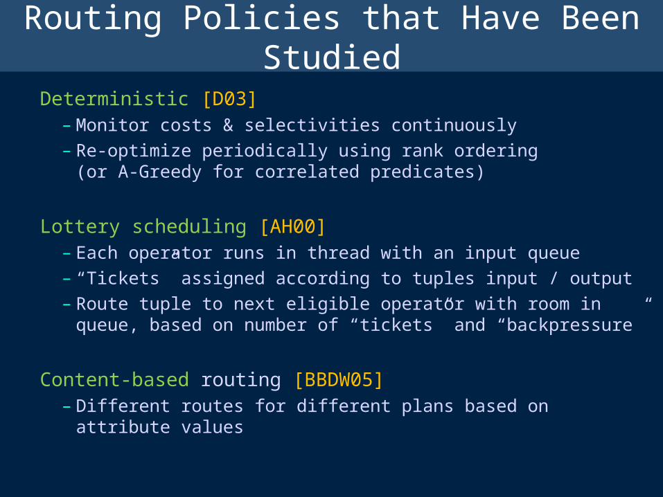
Routing Policies that Have Been Studied
Deterministic [D03]– Monitor costs & selectivities continuously
– Re-optimize periodically using rank ordering(or A-Greedy for correlated predicates)
Lottery scheduling [AH00]– Each operator runs in thread with an input queue
– “Tickets” assigned according to tuples input / output
– Route tuple to next eligible operator with room in queue, based on number of “tickets” and “backpressure”
Content-based routing [BBDW05]– Different routes for different plans based on attribute values

Pipelined Execution Part II:Adaptive Join Processing

Adaptive Join Processing: Outline
Single streaming relation– Left-deep pipelined plans
Multiple streaming relations– Execution strategies for multi-way joins– History-independent execution– History-dependent execution

Left-Deep Pipelined Plans
Simplest method of joining tables– Pick a driver table (R). Call the rest driven tables– Pick access methods (AMs) on the driven tables (scan, hash, or
index)– Order the driven tables– Flow R tuples through the driven tables
For each r R do:look for matches for r in A;for each match a do:
look for matches for <r,a> in B;…
RB
NLJ
C
NLJ
A
NLJ

Adapting a Left-deep Pipelined Plan
Simplest method of joining tables– Pick a driver table (R). Call the rest driven tables– Pick access methods (AMs) on the driven tables– Order the driven tables– Flow R tuples through the driven tables
For each r R do:look for matches for r in A;for each match a do:
look for matches for <r,a> in B;…
Almost identical to selection
ordering
RB
NLJ
C
NLJ
A
NLJ

Adapting the Join Order
Let ci = cost/lookup into i’th driven table,
si = fanout of the lookup
As with selection, cost = |R| x (c1 + s1c2 + s1s2c3)
Caveats:
– Fanouts s1,s2,… can be > 1
– Precedence constraints
– Caching issues
Can use rank ordering, A-greedy for adaptation (subject to the caveats)
RB
NLJ
C
NLJ
A
NLJ
RC
NLJ
B
NLJ
A
NLJ
(c1, s1) (c2, s2) (c3, s3)

Adapting a Left-deep Pipelined Plan
Simplest method of joining tables– Pick a driver table (R). Call the rest driven tables– Pick access methods (AMs) on the driven tables– Order the driven tables– Flow R tuples through the driven tables
For each r R do:look for matches for r in A;for each match a do:
look for matches for <r,a> in B;…
RB
NLJ
C
NLJ
A
NLJ
?

Adapting a Left-deep Pipelined Plan
Key issue: Duplicates
Adapting the choice of driver table
[L+07] Carefully use indexes to achieve this
Adapting the choice of access methods
– Static optimization: explore all possibilities and pick best
– Adaptive: Run multiple plans in parallel for a while, and then pick one and discard the rest [Antoshenkov’ 96]
• Cannot easily explore combinatorial options
SteMs [RDH’03] handle both as well
RB
NLJ
C
NLJ
A
NLJ

Adaptive Join Processing: Outline
Single streaming relation– Left-deep pipelined plans
Multiple streaming relations – Execution strategies for multi-way joins– History-independent execution
• MJoins • SteMs
– History-dependent execution• Eddies with joins• Corrective query processing

Example Join Query & Database
Name Level
Joe Junior
Jen Senior
Name Course
Joe CS1
Jen CS2
Course Instructor
CS2 Smith
select *from students, enrolled, courseswhere students.name = enrolled.name and enrolled.course = courses.course
Students Enrolled
Name Level Course
Joe Junior CS1
Jen Senior CS2
Enrolled Courses
Students Enrolled
Courses
Name Level Course Instructor
Jen Senior CS2 Smith

Symmetric/Pipelined Hash Join [RS86, WA91]
Name Level
Jen Senior
Joe Junior
Name Course
Joe CS1
Jen CS2
Joe CS2
select * from students, enrolled where students.name = enrolled.name
Name Level Course
Jen Senior CS2
Joe Junior CS1
Joe Senior CS2
StudentsEnrolled
Simultaneously builds and probes hash tables on both sides
Widely used: – adaptive query processing
– stream joins
– online aggregation
– …
Naïve version degrades to NLJ once memory runs out– Quadratic time complexity
– memory needed = sum of inputs
Improved by XJoins [UF 00], Tukwila DPJ [IFFLW 99]

Multi-way Pipelined Joins over Streaming Relations
Three alternatives– Using binary join operators
– Using a single n-ary join operator (MJoin) [VNB’03]
– Using unary operators [RDH’03]

Name Level
Jen Senior
Joe Junior
Name Course
Joe CS1
Jen CS2
Enrolled
HashTableE.Name
HashTableS.Name
Students
Course Instructor
CS2 Smith
HashTableE.Course
HashTableC.course
Courses
Name Level Course
Jen Senior CS2
Joe Junior CS1
Name Level Course Instructor
Jen Senior CS2 SmithMaterialized state that depends on the query plan used
History-dependent !
Jen Senior CS2

Multi-way Pipelined Joins over Streaming Relations
Three alternatives
– Using binary join operatorsHistory-dependent execution
Hard to reason about the impact of adaptation
May need to migrate the state when changing plans
– Using a single n-ary join operator (MJoin) [VNB’03]
– Using unary operators [RDH’03]

Name Course
Joe CS1
Jen CS2
Name Level
Joe Junior
Jen Senior
Students
HashTableS.Name
HashTableE.Name
Enrolled
Name Level Course Instructor
Jen Senior CS2 Smith
Name Course
Joe CS1
Jen CS2
HashTableE.Course
HashTableC.course
Courses
Probing Sequences Students tuple: Enrolled, then Courses Enrolled tuple: Students, then Courses Courses tuple: Enrolled, then Students
ProbeProbe
Probe
Hash tables contain all tuples that arrived so far Irrespective of the probing sequences usedHistory-independent execution !
Course Instructor
CS2 Smith
Jen CS2 SmithJen CS2 Senior

Multi-way Pipelined Joins over Streaming Relations
Three alternatives
– Using binary join operatorsHistory-dependent execution
– Using a single n-ary join operator (MJoin) [VNB’03]History-independent execution
Well-defined state easy to reason about
– Especially in data stream processing
Performance may be suboptimal [DH’04]
– No intermediate tuples stored need to recompute
– Using unary operators [RDH’03]
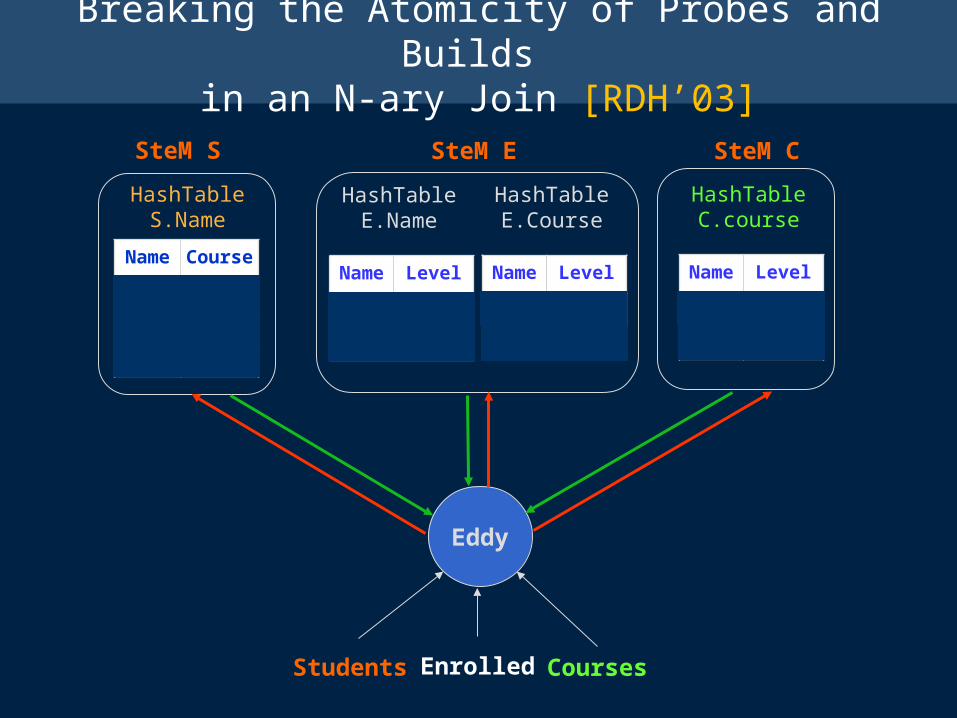
Breaking the Atomicity of Probes and Builds in an N-ary Join [RDH’03]
Name Level
Jen Senior
Joe Junior
Name Course
Joe CS1
Jen CS2
Joe CS2
Students
HashTableS.Name
HashTableE.Name
Enrolled
Name Level
Jen Senior
Joe Junior
HashTableE.Course
Name Level
Jen Senior
Joe Junior
HashTableC.course
Courses
Eddy
SteM S SteM E SteM C

Multi-way Pipelined Joins over Streaming Relations
Three alternatives
– Using binary join operatorsHistory-dependent execution
– Using a single n-ary join operator (MJoin) [VNB’03]History-independent execution
Well-defined state easy to reason about
– Especially in data stream processing
Performance may be suboptimal [DH’04]
– No intermediate tuples stored need to recompute
– Using unary operators [RDH’03]Similar to MJoins, but enables additional adaptation

Adaptive Join Processing: Outline
Single streaming relation– Left-deep pipelined plans
Multiple streaming relations – Execution strategies for multi-way joins– History-independent execution
• MJoins • SteMs
– History-dependent execution• Eddies with joins• Corrective query processing
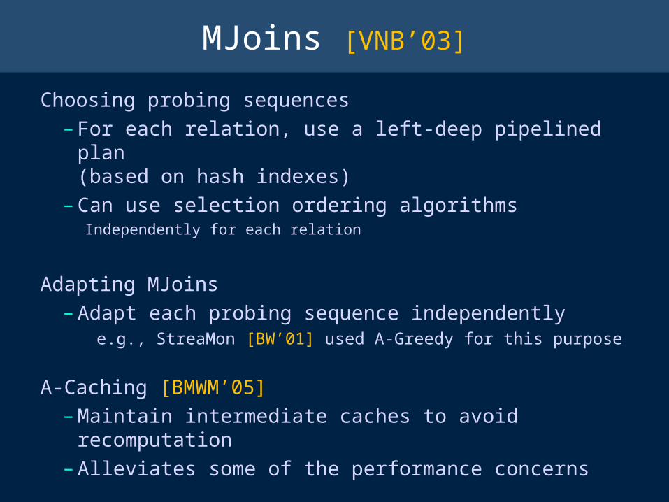
MJoins [VNB’03]
Choosing probing sequences– For each relation, use a left-deep pipelined plan
(based on hash indexes)– Can use selection ordering algorithms
Independently for each relation
Adapting MJoins– Adapt each probing sequence independently
e.g., StreaMon [BW’01] used A-Greedy for this purpose
A-Caching [BMWM’05]– Maintain intermediate caches to avoid recomputation– Alleviates some of the performance concerns

State Modules (SteMs) [RDH’03]
SteM is an abstraction of a unary operator– Encapsulates the state, access methods and the operations on a
single relation
By adapting the routing between SteMs, we can – Adapt the join ordering (as before)– Adapt access method choices– Adapt join algorithms
• Hybridized join algorithms – e.g. on memory overflow, switch from hash join index join
• Much larger space of join algorithms– Adapt join spanning trees
Also useful for sharing state across joins– Advantageous for continuous queries [MSHR’02, CF’03]

Adaptive Join Processing: Outline
Single streaming relation– Left-deep pipelined plans
Multiple streaming relations– Execution strategies for multi-way joins– History-independent execution
• MJoins • SteMs
– History-dependent execution• Eddies with binary joins
– State management using STAIRs• Corrective query processing

Eddies with Binary Joins [AH’00]
Students Enrolled
Output
Courses
E C
S E EddySEC
S E
E C
Output
S.Name like “..”s1
For correctness, must obey routing constraints !!

Eddies with Binary Joins [AH’00]
Students Enrolled
Output
Courses
E C
S E EddySEC
S E
E C
Output
S.Name like “..”e1
For correctness, must obey routing constraints !!
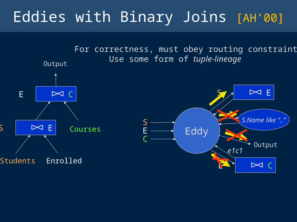
Eddies with Binary Joins [AH’00]
Students Enrolled
Output
Courses
E C
S E EddySEC
S E
E C
Output
S.Name like “..”
e1c1
For correctness, must obey routing constraints !! Use some form of tuple-lineage

Eddies with Binary Joins [AH’00]
Students Enrolled
Output
Courses
E C
S E EddySEC
S E
E C
Output
S.Name like “..”
Can use any join algorithmsBut, pipelined operators preferred Provide quick feedback

Eddies with Symmetric Hash Joins
Eddy
SE
COutput
S E
HashTableS.Name
HashTableE.Name
E C
HashTableE.Course
HashTableC.Course
Joe Jr
Jen Sr
CS2 Smith
Joe CS1
Joe Jr CS1
Jen CS2
Jen CS2 Smith

Burden of Routing History [DH’04]
Eddy
SE
COutput
S E
HashTableS.Name
HashTableE.Name
E C
HashTableE.Course
HashTableC.Course
Joe Jr
Jen Sr
CS2 Smith
Joe CS1
Joe Jr CS1
Jen CS2
Jen CS2 Smith
As a result of routing decisions,state gets embedded inside the operators
History-dependent execution !!

Modifying State: STAIRs [DH’04]
Observation:– Changing the operator ordering not sufficient– Must allow manipulation of state
New operator: STAIR– Expose join state to the eddy
• By splitting a join into two halves– Provide state management primitives
• That guarantee correctness of execution• Able to lift the burden of history
– Enable many other adaptation opportunities• e.g. adapting spanning trees, selective caching, pre-
computation

Recap: Eddies with Binary Joins
Routing constraints enforced using tuple-level lineage
Must choose access methods, join spanning tree beforehand– SteMs relax this restriction [RDH’03]
The operator state makes the behavior unpredictable– Unless only one streaming relation
Routing policies explored are same as for selections– Can tune policy for interactivity metric [RH’02]

Adaptive Join Processing: Outline
Single streaming relation– Left-deep pipelined plans
Multiple streaming relations – Execution strategies for multi-way joins– History-independent execution
• MJoins • SteMs
– History-dependent execution• Eddies with binary joins
– State management using STAIRs• Corrective query processing
F(fid,from,to,when)
F0T(ssn,flight)
T0C(parent,num)
C0
F1T1 C1
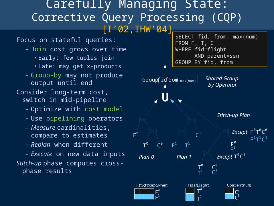
Carefully Managing State:Corrective Query Processing (CQP) [I’02,IHW’04]
Focus on stateful queries:– Join cost grows over time
• Early: few tuples join
• Late: may get x-products
– Group-by may not produce output until end
Consider long-term cost, switch in mid-pipeline– Optimize with cost model– Use pipelining operators– Measure cardinalities,
compare to estimates– Replan when different– Execute on new data inputs
Stitch-up phase computes cross-phase results
Group[fid,from] max(num)
F0
T0 C0
Plan 0
1C
T1F1
Plan 1
Shared Group-by Operator
U
T0 C0
T1 C1
F0
F1
T0C0Except
T0C0Except F0
T1C1F1
Stitch-up Plan
SELECT fid, from, max(num)FROM F, T, CWHERE fid=flight AND parent=ssnGROUP BY fid, from

CQP Discussion
Each plan operates on a horizontal partition: Clean algebraic interpretation!
Easy to extend to more complex queries– Aggregation, grouping, subqueries, etc.
Separates two factors, conservatively creates state:– Scheduling is handled by pipelined operators
– CQP chooses plans using long-term cost estimation
– Postpones cross-phase results to final phaseAssumes settings where computation cost, state are the bottlenecks
– Contrast with STAIRS, which move state around once it’s created!

Putting it all in Context
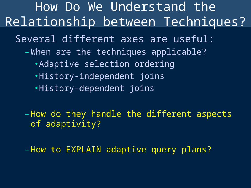
How Do We Understand theRelationship between Techniques?
Several different axes are useful:– When are the techniques applicable?
• Adaptive selection ordering• History-independent joins• History-dependent joins
– How do they handle the different aspects of adaptivity?
– How to EXPLAIN adaptive query plans?

Adaptivity Loop
Measure what ? Cardinalities/selectivities, operator costs, resource utilization
Measure when ? Continuously (eddies); using a random sample (A-greedy); at materialization points (mid-query reoptimization)
Measurement overhead ? Simple counter increments (mid-query) to very high
ActuateActuate
PlanPlanAnalyzeAnalyze
MeasureMeasure

Adaptivity Loop
Analyze/replan what decisions ? (Analyze actual vs. estimated selectivities) Evaluate costs of alternatives and switching (keep state in mind)Analyze / replan when ? Periodically; at materializations (mid-query); at conditions (A-greedy)
Plan how far ahead ?
Next tuple; batch; next stage (staged); possible remainder of plan (CQP)Planning overhead ? Switch stmt (parametric) to dynamic programming (CQP, mid-query)
ActuateActuateMeasureMeasure
PlanPlanAnalyzeAnalyze

Adaptivity Loop
Actuation: How do they switch to the new plan/new routing strategy ?
Actuation overhead ?
At the end of pipelines free (mid-query)
During pipelines:
History-independent Essentially free (selections, MJoins)
History-dependent May need to migrate state (STAIRs, CAPE)
MeasureMeasure
PlanPlanAnalyzeAnalyze
ActuateActuate
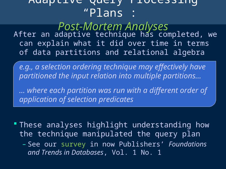
Adaptive Query Processing “Plans”: Post-Mortem Analyses
After an adaptive technique has completed, we can explain what it did over time in terms of data partitions and relational algebra
e.g., a selection ordering technique may effectively have partitioned the input relation into multiple partitions…
… where each partition was run with a different order of application of selection predicates
These analyses highlight understanding how the technique manipulated the query plan– See our survey in now Publishers’ Foundations and Trends in
Databases, Vol. 1 No. 1

Research Roundup

Measurement & Models
Combining static and runtime measurement
Finding the right model granularity / measurement timescale– How often, how heavyweight? Active probing?
Dealing with correlation in a tractable way
There are clear connections here to:– Online algorithms
– Machine learning and control theory
• Bandit problems
• Reinforcement learning
– Operations research scheduling

Understanding Execution Space
Identify the “complete” space of post-mortem executions:– Partitioning
– Caching
– State migration
– Competition & redundant work
– Sideways information passing
– Distribution / parallelism!
What aspects of this space are important? When?– A buried lesson of AQP work: “non-Selingerian” plans can win big!
– Can we identify robust plans or strategies?
Given this (much!) larger plan space, navigate it efficiently– Especially on-the-fly

Wrap-up
Adaptivity is the future (and past!) of query processing
Lessons and structure emerging– The adaptivity “loop” and its separable components
Relationship between measurement, modeling / planning, actuation
– Horizontal partitioning “post-mortems” as a logical framework for understanding/explaining adaptive execution in a post-mortem sense
– Selection ordering as a clean “kernel”, and its limitations
– The critical and tricky role of state in join processing
A lot of science and engineering remain!!!

References
[A-D03] R. Arpaci-Dusseau. Runtime Adaptation in River. ACM TOCS 2003. [AH’00] R. Avnur, J. M. Hellerstein: Eddies: Continuously Adaptive Query Processing SIGMOD
Conference 2000: 261-272 [Antoshenkov93] G. Antoshenkov: Dynamic Query Optimization in Rdb/VMS. ICDE 1993: 538-547. [BBD’05] S. Babu, P. Bizarro, D. J. DeWitt. Proactive Reoptimization. VLDB 2005: 107-118 [BBDW’05] P. Bizarro, S. Babu, D. J. DeWitt, J. Widom: Content-Based Routing: Different Plans for
Different Data. VLDB 2005: 757-768 [BC02] N. Bruno, S. Chaudhuri: Exploiting statistics on query expressions for optimization. SIGMOD
Conference 2002: 263-274 [BC05] B. Babcock, S. Chaudhuri: Towards a Robust Query Optimizer: A Principled and Practical
Approach. SIGMOD Conference 2005: 119-130 [BMMNW’04] S. Babu, et al: Adaptive Ordering of Pipelined Stream Filters. SIGMOD Conference 2004:
407-418 [CDHW06] Flow Algorithms for Two Pipelined Filter Ordering Problems; Anne Condon, Amol Deshpande,
Lisa Hellerstein, and Ning Wu. PODS 2006. [CDY’95] S. Chaudhuri, U. Dayal, T. W. Yan: Join Queries with External Text Sources: Execution and
Optimization Techniques. SIGMOD Conference 1995: 410-422 [CG94] R. L. Cole, G. Graefe: Optimization of Dynamic Query Evaluation Plans. SIGMOD Conference
1994: 150-160. [CF03] S. Chandrasekaran, M. Franklin. Streaming Queries over Streaming Data; VLDB 2003 [CHG02] F. C. Chu, J. Y. Halpern, J. Gehrke: Least Expected Cost Query Optimization: What Can We
Expect? PODS 2002: 293-302 [CN97] S. Chaudhuri, V. R. Narasayya: An Efficient Cost-Driven Index Selection Tool for Microsoft SQL
Server. VLDB 1997: 146-155

References (2)
[CR94] C-M Chen, N. Roussopoulos: Adaptive Selectivity Estimation Using Query Feedback. SIGMOD Conference 1994: 161-172
[DGHM’05] A. Deshpande, C. Guestrin, W. Hong, S. Madden: Exploiting Correlated Attributes in Acquisitional Query Processing. ICDE 2005: 143-154
[DGMH’05] A. Deshpande, et al.: Model-based Approximate Querying in Sensor Networks. In VLDB Journal, 2005
[DH’04] A. Deshpande, J. Hellerstein: Lifting the Burden of History from Adaptive Query Processing. VLDB 2004.
[EHJKMW’96] O. Etzioni, et al: Efficient Information Gathering on the Internet. FOCS 1996: 234-243 [GW’00] R. Goldman, J. Widom: WSQ/DSQ: A Practical Approach for Combined Querying of
Databases and the Web. SIGMOD Conference 2000: 285-296 [INSS92] Y. E. Ioannidis, R. T. Ng, K. Shim, T. K. Sellis: Parametric Query Optimization. VLDB 1992. [IHW04] Z. G. Ives, A. Y. Halevy, D. S. Weld: Adapting to Source Properties in Data Integration
Queries. SIGMOD 2004. [K’01] M.S. Kodialam. The throughput of sequential testing. In Integer Programming and
Combinatorial Optimization (IPCO) 2001. [KBZ’86] R. Krishnamurthy, H. Boral, C. Zaniolo: Optimization of Nonrecursive Queries. VLDB 1986. [KD’98] N. Kabra, D. J. DeWitt: Efficient Mid-Query Re-Optimization of Sub-Optimal Query Execution
Plans. SIGMOD Conference 1998: 106-117 [KKM’05] H. Kaplan, E. Kushilevitz, and Y. Mansour. Learning with attribute costs. In ACM STOC,
2005. [KNT89] Masaru Kitsuregawa, Masaya Nakayama and Mikio Takagi, "The Effect of Bucket Size
Tuning in the Dynamic Hybrid GRACE Hash Join Method”. VLDB 1989.

References (3) [LEO 01] M. Stillger, G. M. Lohman, V. Markl, M. Kandil: LEO - DB2's LEarning Optimizer. VLDB 2001. [L+07] Quanzhong Li et al. Adaptively Reordering Joins during Query Execution; ICDE 2007. [MRS+04] Volker Markl, et al.: Robust Query Processing through Progressive Optimization. SIGMOD
Conference 2004: 659-670 [MSHR’02] S. Madden, M. A. Shah, J. M. Hellerstein, V. Raman: Continuously adaptive continuous
queries over streams. SIGMOD Conference 2002: 49-60 [NKT88] M. Nakayama, M. Kitsuregawa, and M. Takagi. Hash partitioned join method using dynamic
destaging strategy. In VLDB 1988. [PCL93a] H. Pang, M. J. Carey, M. Livny: Memory-Adaptive External Sorting. VLDB 1993: 618-629 [PCL93b] H. Pang, M. J. Carey, M. Livny: Partially Preemptive Hash Joins. SIGMOD Conference
1993. [RH’05] N. Reddy, J. Haritsa: Analyzing Plan Daigrams of Database Query Optimizers; VLDB 2005. [SF’01] M.A. Shayman and E. Fernandez-Gaucherand: Risk-sensitive decision-theoretic diagnosis.
IEEE Trans. Automatic Control, 2001. [SHB04] M. A. Shah, J. M. Hellerstein, E. Brewer. Highly-Available, Fault-Tolerant, Parallel Dataflows ,
SIGMOD, June 2004. [SHCF03] M. A. Shah, J. M. Hellerstein, S. Chandrasekaran and M. J. Franklin. Flux: An Adaptive
Partitioning Operator for Continuous Query Systems, ICDE, March 2003. [SMWM’06] U. Srivastava, K. Munagala, J. Widom, R. Motwani: Query Optimization over Web
Services; VLDB 2006. [TD03] F. Tian, D. J. Dewitt. Tuple Routing Strategies for Distributed Eddies. VLDB 2003. [UFA’98] T. Urhan, M. J. Franklin, L. Amsaleg: Cost Based Query Scrambling for Initial Delays.
SIGMOD Conference 1998: 130-141 [UF 00] T. Urhan, M. J. Franklin: XJoin: A Reactively-Scheduled Pipelined Join Operator. IEEE Data
Eng. Bull. 23(2): 27-33 (2000) [VNB’03] S. Viglas, J. F. Naughton, J. Burger: Maximizing the Output Rate of Multi-Way Join Queries
over Streaming Information Sources. VLDB 2003: 285-296 [WA’91] A. N. Wilschut, P. M. G. Apers: Dataflow Query Execution in a Parallel Main-Memory
Environment. PDIS 1991: 68-77


