
AMERICAN JOURNAL OF EPIDEMIOLOGYCopyright © 1988 by The Johns Hopkins University School of Hygiene and Public HealthAll rights reserved
Vol. 127, No. 5Printed in U.S.A.
THE ECOLOGICAL FALLACY
STEVEN PIANTADOSI,12 DAVID P. BYAR,1 AND SYLVAN B. GREEN1
The purpose of this paper is to emphasizefor epidemiologists the possibility of seriouserrors resulting from inferences based onecological analyses. Variables that describegroups of individuals, rather than the in-dividuals themselves, are termed "ecologi-cal" and are often used when the analysisof individuals' data is not possible (1). Eco-logical analyses may be preferred when 1)variables are more conveniently defined ormeasured on groups because the analysison individuals would require excessive timeor extensive data gathering; 2) ecologicalanalyses permit study of a wider range ofvalues for the independent variable, as ininternational studies of diet; 3) the preci-sion of aggregate measures like alcohol con-sumption is likely to be higher for groupsthan for individuals; and 4) population re-sponses such as smoking quit rates may beof primary interest. Frequently, more thanone reason applies. For example, some ofthe evidence favoring environmental anddietary causes of cancer comes from thecomparison of incidence or mortality rateswith average levels of risk factors measuredon culturally or geographically definedgroups of individuals. The first three rea-sons are relevant to this type of study.
We assume in this paper that measure-ments on individuals are not available, asin the diet and cancer example, since whenthis information is known, it might be usedin place of, or to correct for biases in, the
1 Biometry Branch, Division of Cancer Preventionand Control, NCI, NIH, Bethesda, MD.
2 Current address: The Johns Hopkins University,Department of Oncology/Biostatistics, 550 N. Broad-way, Suite 1103, Baltimore, MD 21205. (Reprint re-quests to Dr. Steven Piantadosi at this address.)
The authors thank Dr. Sholom Wacholder, Dr.Charles Brown, and Dr. Peter Greenwald for helpfulcomments and Jennifer Gaegler for manuscript assist-
ecological analysis. Serious errors can re-sult when an investigator makes the seem-ingly natural assumption that the infer-ences from an ecological analysis must per-tain either to the individuals within thegroups or to individuals across groups. Afrequently cited early example of an ecolog-ical inference was Durkheim's study of thecorrelation between suicide rates and reli-gious denominations in Prussia (2) inwhich the suicide rate was observed to becorrelated with the number of Protestants.However, it could as well have been theCatholics who were committing suicide inlargely Protestant provinces. The potentialfalsity of ecological inferences, at least inthe case of simple correlations, was pointedout by Robinson (3), who gave it the name"ecological fallacy" and provided the math-ematical relation, without proof, betweenthe ecological correlation and the individ-ual correlation across all groups. Duncan etal. (4) have extended the equations to in-clude simple linear regression coefficients.The dangers of inferences about individualsfrom ecological studies have been empha-sized by some investigators (5-7), whileothers (8-11) have sought to minimize theconcern over the possible biases in ecolog-ical analyses, proposing alternatives or de-lineating circumstances in which ecologicalinferences are justified (e.g., certain linearregression models when data on individualsare available). Firebaugh (11) gives a par-ticularly thorough discussion and list ofreferences related to this aspect of the prob-lem.
Although there has been a persistent in-terest in the problems associated with eco-logical analyses in the social science liter-ature, the impression seems to remain, evenamong seasoned epidemiologists, that eco-logical analyses may not have large biases,
893
at University of C
alifornia, Los Angeles on A
ugust 3, 2011aje.oxfordjournals.org
Dow
nloaded from
894 PIANTADOSI ET AL.
at least in certain cases. Such impressionsresult, in part, from the nonintuitive soundof serious disparity between group level andindividual level statistics. Our goal is toprovide convincing evidence, intuitively,mathematically, and empirically, of thepossibility of important bias in ecologicalanalyses and to clarify some recent workon this topic. We present a hypotheticalexample of the ecological fallacy and a sim-ple derivation of the relation between theindividual correlation and the ecologicalcorrelation. We extend this derivation tooutline the relation between the individualregression slope and the ecological regres-sion slope. In addition, theoretical obser-vations are supported by an ecologicalanalysis of correlations and regression coef-ficients for a set of real data, using variablesoften encountered in epidemiologic prac-tice.
HYPOTHETICAL EXAMPLE
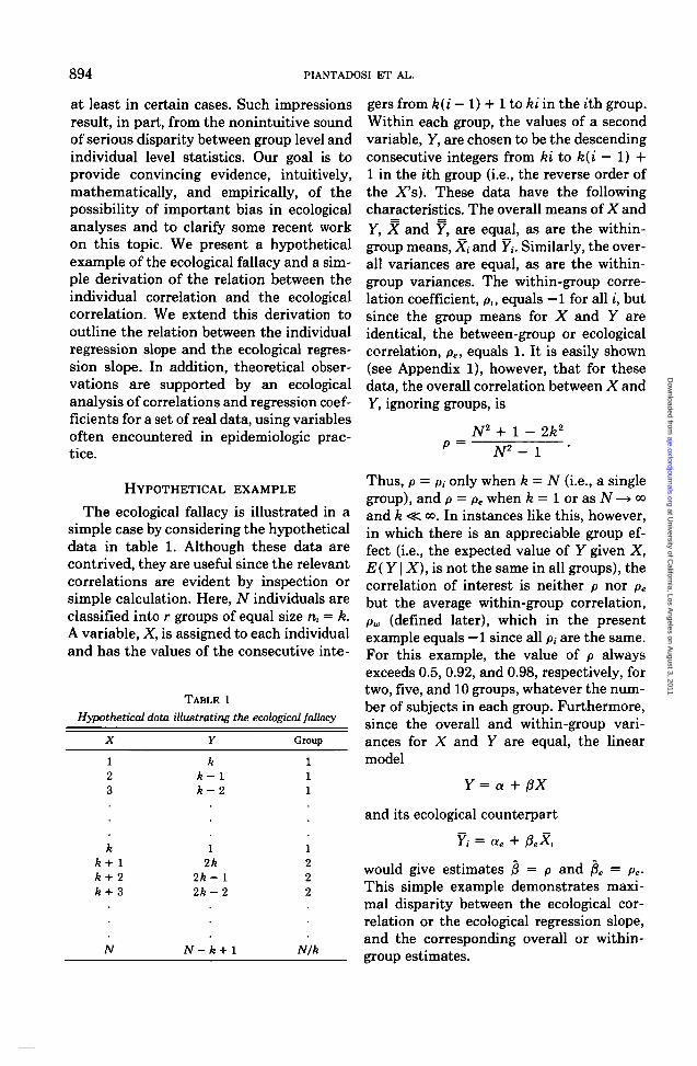
The ecological fallacy is illustrated in asimple case by considering the hypotheticaldata in table 1. Although these data arecontrived, they are useful since the relevantcorrelations are evident by inspection orsimple calculation. Here, N individuals areclassified into r groups of equal size n, = k.A variable, X, is assigned to each individualand has the values of the consecutive inte-
TABLE l
Hypothetical data illustrating the ecological fallacy
X Y Group
123
kk + 1k + 2k + 3
kk-k-
12k
2k-2k-
12
12
111
1222
gers from k(i — 1) + 1 to ki in the ith group.Within each group, the values of a secondvariable, Y, are chosen to be the descendingconsecutive integers from ki to k{i — 1) +1 in the ith group (i.e., the reverse order ofthe X's). These data have the followingcharacteristics. The overall means of X andY, X and Y, are equal, as are the within-group means, X, and Y,. Similarly, the over-all variances are equal, as are the within-group variances. The within-group corre-lation coefficient, p,, equals —1 for all i, butsince the group means for X and Y areidentical, the between-group or ecologicalcorrelation, pe, equals 1. It is easily shown(see Appendix 1), however, that for thesedata, the overall correlation between X andY, ignoring groups, is
P =AT2 + 1 - 2k2
N2 - 1
N N-k+1 N/k
Thus, p = pc only when k = N (i.e., a singlegroup), and p = pe when k = 1 or as N —* ooand k <K oo. In instances like this, however,in which there is an appreciable group ef-fect (i.e., the expected value of Y given X,E( Y | X), is not the same in all groups), thecorrelation of interest is neither p nor pe
but the average within-group correlation,pw (defined later), which in the presentexample equals —1 since all p, are the same.For this example, the value of p alwaysexceeds 0.5, 0.92, and 0.98, respectively, fortwo, five, and 10 groups, whatever the num-ber of subjects in each group. Furthermore,since the overall and within-group vari-ances for X and Y are equal, the linearmodel
Y= a + 0X
and its ecological counterpart
Y, = ae + (3eX
would give estimates /J = p and (3e = Pe-
This simple example demonstrates maxi-mal disparity between the ecological cor-relation or the ecological regression slope,and the corresponding overall or within-group estimates.
at University of C
alifornia, Los Angeles on A
ugust 3, 2011aje.oxfordjournals.org
Dow
nloaded from
THE ECOLOGICAL FALLACY 895
DERIVATION OF GENERAL RELATIONS
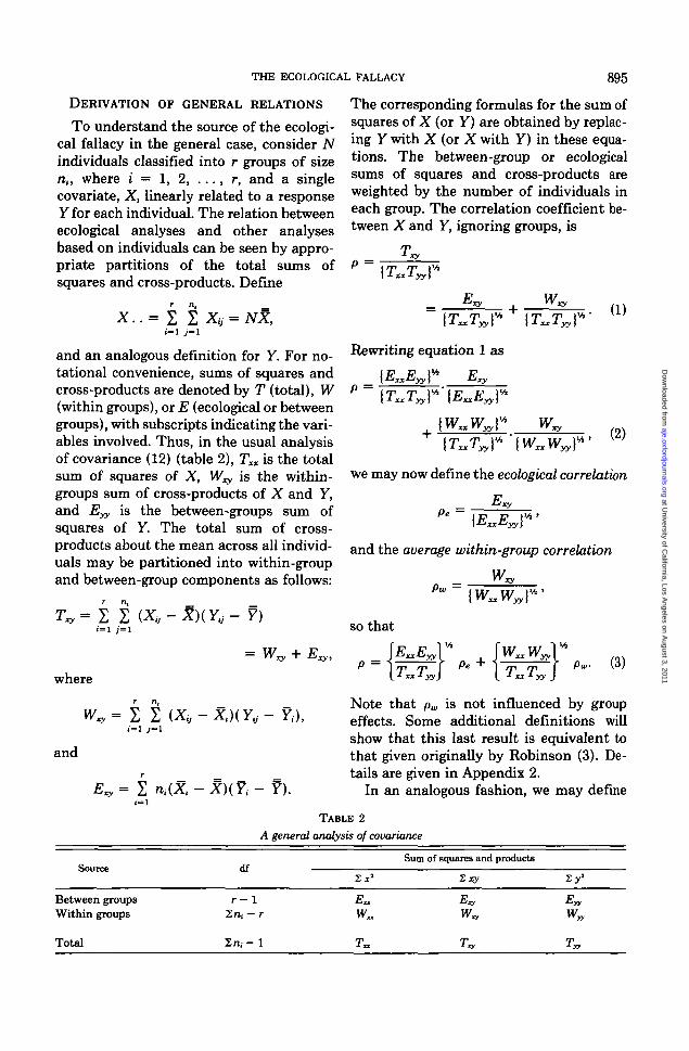
To understand the source of the ecologi-cal fallacy in the general case, consider Nindividuals classified into r groups of sizen,, where i = 1, 2, . . . , r, and a singlecovariate, X, linearly related to a responseY for each individual. The relation betweenecological analyses and other analysesbased on individuals can be seen by appro-priate partitions of the total sums ofsquares and cross-products. Define
X..=
and an analogous definition for Y. For no-tational convenience, sums of squares andcross-products are denoted by T (total), W(within groups), or E (ecological or betweengroups), with subscripts indicating the vari-ables involved. Thus, in the usual analysisof covariance (12) (table 2), Txx is the totalsum of squares of X, W^ is the within-groups sum of cross-products of X and Y,and Eyy is the between-groups sum ofsquares of Y. The total sum of cross-products about the mean across all individ-uals may be partitioned into within-groupand between-group components as follows:
=1 ; = 1.j- Y)
= WZy+ EXy,
where
and
i = l 7=1
r v \l V V \
I - Y).
The corresponding formulas for the sum ofsquares of X (or Y) are obtained by replac-ing Y with X (or X with Y) in these equa-tions. The between-group or ecologicalsums of squares and cross-products areweighted by the number of individuals ineach group. The correlation coefficient be-tween X and Y, ignoring groups, is
P = j rp rp >V41 i- xxlyyS
irp rp »ViI J- xxJ-yy)
Rewriting equation 1 as
irp rp jVb •t J- xx-lyyf
(1)
P =
IW W I*
,„ wj" (2)
we may now define the ecological correlation
Pe =
and the average within-group correlation
WxyPw —
so that
P _ j&&}\+tor L •* xxlyy) \_ ixx^yy )
(3)
Note that pw is not influenced by groupeffects. Some additional definitions willshow that this last result is equivalent tothat given originally by Robinson (3). De-tails are given in Appendix 2.
In an analogous fashion, we may define
TABLE 2
A general analysis of covariance
Source
Between groupsWithin groups
Total
df
r - 12ra, — r
Sra,- 1
2 I2
Sum of squares and products
2 x y
Wyy
Tyy
at University of C
alifornia, Los Angeles on A
ugust 3, 2011aje.oxfordjournals.org
Dow
nloaded from
896 PIANTADOSI ET AL.
the regression coefficients
TP - TfT >
1 xx
and
and show that
WPw w ,
WP = 7f Pe + -zr Pw, (4)
-*• xx •* xx
where ft ft, and ft, are the overall regres-sion slope, ecological regression slope, andthe average within-group regression slope,respectively. This can be written
ft = f= 0 - & - ll ft,
T= ft, + — (|8 - ft,), (5)
with the first equality being the relationgiven by Duncan et al. (4).
ANALYSIS OF GENERAL RELATIONS
In the absence of group effects, theregression coefficient of interest is 0,whereas when group effects are present, p*w
is a more appropriate description of thedata. In fact, when group effects are absent,P = ft,, so that ft, is always the regressioncoefficient of interest. The ecological fal-lacy consists of incorrectly assuming that,when group effects are present, ft = ft.
We can see immediately from equation 4that the coefficients of ft and ft sum to 1,so that /3 is always a weighted average ofthe ecological and within-group regressionslopes. The consequence of this is that peither lies between ft and ft, (although theorder of ft and ft, cannot be predicted) or,when there are no group effects, /3 = jSe =ft,. More generally, however, there aregroup effects so that P and ftj are unequal,and thus ft and ft, are also unequal. Forregression coefficients, the notion of sepa-
rating "cross-level" bias into aggregationbias (the difference between p and pe) andspecification bias (the difference between Pand pw) (1) is not meaningful since bothbiases either occur together or not at all, asimplied by Firebaugh (11). In fact, it mayeasily be shown that
WPe-P = -=?(P- PJ,
hixx
further emphasizing that aggregation biasand specification bias do not occur sepa-rately.
The results for correlation coefficientsare similar. The multipliers of pe and pw inequation 3 do not, however, sum to 1, sothat p is not always constrained as P was.For correlations, the ecological fallacy con-sists of incorrectly assuming that pe esti-mates either p or pw.
The point has been correctly made (1,10, 11) that ecological correlations arelikely to be poorer estimates of their indi-vidual counterparts than ecological regres-sion slopes. This is because correlationsdepend on the relative dispersions of X andY and thus are determined by the design ofthe experiment. Note that
WxxPw = Pw\ -7771 pe =
Ex
Selecting groups specifically because theydiffer in X, will tend to increase the vari-ance of Xi compared with the variance ofy,, and therefore increase the ecologicalcorrelation. In the absence of group effectsin regression (P = pe = Pw), the correlationscan nevertheless differ, and the relation ofpe and pw will depend on how the groupsare chosen. Although demonstrating thatPe^O can be useful, its actual value seemsquite arbitrary. If the goal is to make state-ments about Y on the basis of X, then inthis situation, ft is a more useful quantitythan pe.
It has been stated by some writers (seefor example Stavraky (13) and Kleinbaumet al. (14)) that ecological associations arefrequently an overestimate of the magni-
at University of C
alifornia, Los Angeles on A
ugust 3, 2011aje.oxfordjournals.org
Dow
nloaded from
THE ECOLOGICAL FALLACY 897
tude of the underlying individual effects.While this is always possible, we can findno justification for assuming that it is morelikely than the alternative. As noted above,in the absence of group effects, the selectionof groups will affect pw (and may well tendto increase correlations). When group ef-fects do, however, exist (which is quitelikely in epidemiologic studies), the biascan be in either direction.
The concept of group effects in regres-sion can be expressed in other ways. Asstated above, by group effects we mean thatE(Y\X) is not the same in all groups or,equivalently, that j8 # ft, 5 fiw (i.e., there iscross-level bias). Thus, group membershipis related to some confounding factor(s)which affects the observed relation betweenX and Y. Firebaugh (11) addresses thissituation by considering a regression of theform Y = a + ftX + yXi; the presence ofgroup effects implies that 7 5 0. Withoutdata on individuals, this situation cannotbe detected, yet it is quite likely to exist inepidemiologic studies. Of course, if an in-vestigator is aware of potential confoundingvariables measured on the groups, these canbe included in the ecological regression todecrease the bias (10). The issue to consideris how likely are the groups to differ byother (unmeasured) variables.
A confounder can exist on two levels. Avariable could be confounding only on thegroup level, and thus affect both 0 (theoverall slope for X) and ft, (the ecologicalslope for X), but not ft,,. For example, thevariable could be a characteristic of thewhole group rather than the individual(e.g., geographic latitude) or the variablecould be independent of X within groups,but correlated with X across groups. If sucha variable were known, it could be properlyincorporated in an ecological regression.The problem is that variables such as thiscould well exist but not be identified. Ifindividual level data on X and Y were avail-able, individual level regression adjusted forgroup effect would permit unbiased esti-mation of the desired effect of X on Y.
Alternatively, a variable could be con-
founding on both the individual and grouplevels (e.g., age confounding the effect ofdiet). In this situation, information on theconfounder would have to be incorporatedinto the regression whether at the individ-ual level or the ecological level.
In theory, there is a third alternative inwhich a variable is confounding on the in-dividual level but is not confounding inlinear regression at the group level (becausethe variable is uncorrelated with groupmembership). For example, in an investi-gation of the relation of diet to the risk ofcolon cancer, sex is a possible confoundingfactor, but it is conceivable that all groupshave essentially the same sex ratio. In thissituation, ecological regression might bepreferable to unadjusted individual levelregression.
EMPIRICAL STUDY OF ECOLOGICAL
CORRELATIONS
We now consider an ecological analysisof data from the Second National Healthand Nutrition Examination Survey(NHANES II) in which we can compareindividual level and grouped estimates.This study, conducted by the National Cen-ter for Health Statistics between 1976 and1980, was intended to assess the health andnutritional status of the general civiliannoninstitutionalized population of theUnited States (15). Initially, a nationwideprobability sample of approximately 28,000persons was taken with oversampling inthose groups thought to be at high risk ofmalnutrition (low income, preschool chil-dren, and the elderly). A 24-hour dietaryrecall questionnaire was given to a subsetof 13,820 adults. From these records, weselected 11 variables for analysis describingor derived from health history, food fre-quency, and anthropometry (16). Measure-ments were on continuous scales for dietarymeasures, height, weight, age, and bodymass index (weight in kilograms divided bythe square of height in meters), orderedcategories for income and education, andbinary categories for sex and race (table 3).These variables were selected not because
at University of C
alifornia, Los Angeles on A
ugust 3, 2011aje.oxfordjournals.org
Dow
nloaded from
898 PIANTADOSI ET AL.
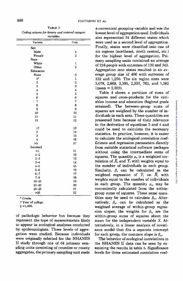
TABLE 3
Coding scheme for binary and ordered categoryvariables
Variable
SexMaleFemale
RaceWhiteOther
EducationNone
1*23456789
101112
I t234
>5Income^
< 11-22-33-44-55-66-77-9
10-1515-2020-25>25
Code
12
12
0123456789
101112
1314151617
111213141516171819202122
* Grade.t Year of college.$ XI,000.
of pathologic behavior but because theyrepresent the type of measurements likelyto appear in ecological analyses conductedby epidemiologists. Three levels of aggre-gation were studied. Because individualswere originally selected for the NHANESII study through one of 64 primary sam-pling units consisting of counties or countyaggregates, the primary sampling unit made
a convenient grouping variable and was thelowest level of aggregation used. Individualsalso represented 34 different states whichwere used as a second level of aggregation.Finally, states were classified into one ofsix regions (northeast, north central, etc.)for the highest level of aggregation. Pri-mary sampling units contained an averageof 216 people with extremes of 130 and 343.Aggregation into states resulted in an av-erage group size of 406 with extremes of132 and 1,250. The six region sizes were3,078, 2,869, 3,395, 2,333, 763, and 1,382(mean = 2,303).
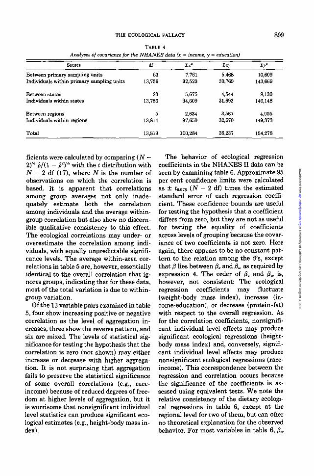
Table 4 shows a partition of sums ofsquares and cross-products for the vari-ables income and education (highest gradeattained). The between-group sums ofsquares are weighted by the number of in-dividuals in each area. These quantities arepresented here because of their relevanceto the derivation of equations 3 and 4 andcould be used to calculate the necessarystatistics. In practice, however, it is easierto calculate the ecological correlation coef-ficients and regression parameters directlyfrom suitable statistical software packageswithout using the intermediate sums ofsquares. The quantity pe is a weighted cor-relation of Xi and Y, with weights equal tothe number of individuals in each group.Similarly, /3e can be calculated as theweighted regression of Y; on X, withweights equal to the number of individualsin each group. The quantity pw may beconveniently calculated from the within-group sums of squares. These same quan-tities may be used to calculate /3M. Alter-natively, f3w can be calculated as theweighted average of within-group regres-sion slopes; the weights for pw are thewithin-group sums of squares about themean for the independent variable X. Al-ternatively, in a linear analysis of covari-ance model that fits a separate interceptfor each group, the common slope is /3W.
The behavior of ecological correlations inthe NHANES II data can be seen by ex-amining the results in table 5. Significancelevels for these estimated correlation coef-
at University of C
alifornia, Los Angeles on A
ugust 3, 2011aje.oxfordjournals.org
Dow
nloaded from
THE ECOLOGICAL FALLACY 899
TABLE 4
Analyses of covariance for the NHANES data (x = income, y = education)
Source df
Between primary sampling unitsIndividuals within primary sampling units
Between statesIndividuals within states
Between regionsIndividuals within regions
Total
6313,756
3313,786
513,814
7,76192,523
5,67594,609
2,63497,650
5,46830,769
4,54431,693
3,56732,670
10,609143,669
8,130146,148
4,905149,373
13,819 100,284 36,237 154,278
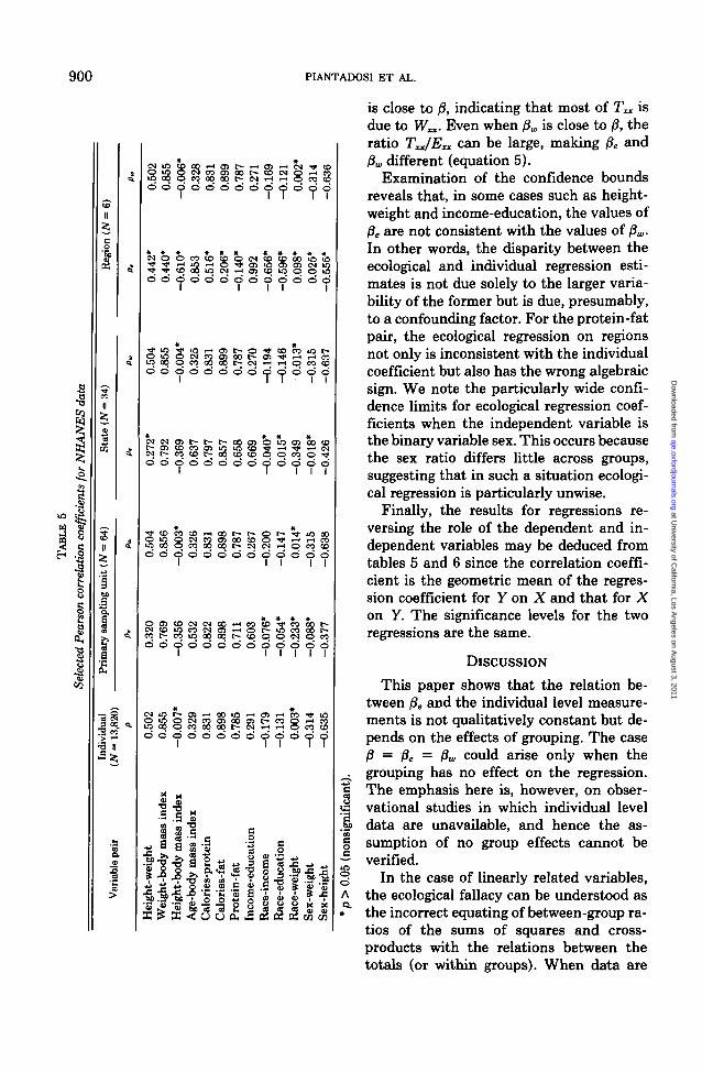
ficients were calculated by comparing {N —2)* p/(l - p2)* with the t distribution withN — 2 df (17), where N is the number ofobservations on which the correlation isbased. It is apparent that correlationsamong group averages not only inade-quately estimate both the correlationamong individuals and the average within-group correlation but also show no discern-ible qualitative consistency to this effect.The ecological correlations may under- oroverestimate the correlation among indi-viduals, with equally unpredictable signifi-cance levels. The average within-area cor-relations in table 5 are, however, essentiallyidentical to the overall correlation that ig-nores groups, indicating that for these data,most of the total variation is due to within-group variation.
Of the 13 variable pairs examined in table5, four show increasing positive or negativecorrelation as the level of aggregation in-creases, three show the reverse pattern, andsix are mixed. The levels of statistical sig-nificance for testing the hypothesis that thecorrelation is zero (not shown) may eitherincrease or decrease with higher aggrega-tion. It is not surprising that aggregationfails to preserve the statistical significanceof some overall correlations (e.g., race-income) because of reduced degrees of free-dom at higher levels of aggregation, but itis worrisome that nonsignificant individuallevel statistics can produce significant eco-logical estimates (e.g., height-body mass in-dex).
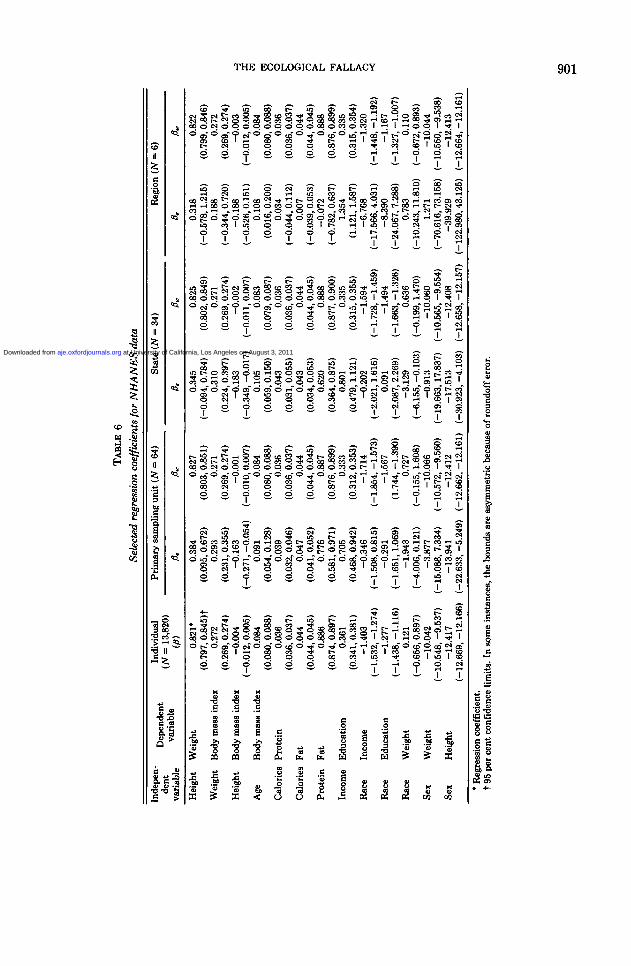
The behavior of ecological regressioncoefficients in the NHANES II data can beseen by examining table 6. Approximate 95per cent confidence limits were calculatedas ± to.975 (N - 2 df) times the estimatedstandard error of each regression coeffi-cient. These confidence bounds are usefulfor testing the hypothesis that a coefficientdiffers from zero, but they are not as usefulfor testing the equality of coefficientsacross levels of grouping because the covar-iance of two coefficients is not zero. Hereagain, there appears to be no constant pat-tern to the relation among the fl's, exceptthat P lies between ft, and ft,, as required byexpression 4. The order of ft, and (lw is,however, not consistent: The ecologicalregression coefficients may fluctuate(weight-body mass index), increase (in-come-education), or decrease (protein-fat)with respect to the overall regression. Asfor the correlation coefficients, nonsignifi-cant individual level effects may producesignificant ecological regressions (height-body mass index) and, conversely, signifi-cant individual level effects may producenonsignificant ecological regressions (race-income). This correspondence between theregression and correlation occurs becausethe significance of the coefficients is as-sessed using equivalent tests. We note therelative consistency of the dietary ecologi-cal regressions in table 6, except at theregional level for two of them, but can offerno theoretical explanation for the observedbehavior. For most variables in table 6, f3w
at University of C
alifornia, Los Angeles on A
ugust 3, 2011aje.oxfordjournals.org
Dow
nloaded from
900 PIANTADOSI ET AL.
a
1I
U_>CO
I18
II
I
I
SII
.S"a
•C
a.
il
O w Do o o o o d o o o o o o o
NOOM^tOCKNtoioOifllo
o o c i o o o o o o o o o d
Oq
d o d o d d o o o o oI I I
o o o o o o o o o o o o dI I I I !
COCDON
qcoq q
d o c J o o o o d d o o d ©I I I I I
d©I I
C l ^ ? ^ y 00 ^ 1 ^ ^ ^^ C ^ ^ ^ t ^ C J 00 ^ *C O t > C O l C O O O O t * - C D O © C ^ O C Oo o p o o o o o o p o o o
I I
S 8 CO
d o o d dCO CD
£ a
•r? hfi *fe
"§•§'§ I
is close to j8, indicating that most of T^ isdue to Wn- Even when f)w is close to (8, theratio T^/Exx can be large, making ft. and(3a, different (equation 5).
Examination of the confidence boundsreveals that, in some cases such as height-weight and income-education, the values ofPe are not consistent with the values of flw.In other words, the disparity between theecological and individual regression esti-mates is not due solely to the larger varia-bility of the former but is due, presumably,to a confounding factor. For the protein-fatpair, the ecological regression on regionsnot only is inconsistent with the individualcoefficient but also has the wrong algebraicsign. We note the particularly wide confi-dence limits for ecological regression coef-ficients when the independent variable isthe binary variable sex. This occurs becausethe sex ratio differs little across groups,suggesting that in such a situation ecologi-cal regression is particularly unwise.
Finally, the results for regressions re-versing the role of the dependent and in-dependent variables may be deduced fromtables 5 and 6 since the correlation coeffi-cient is the geometric mean of the regres-sion coefficient for Y on X and that for Xon Y. The significance levels for the tworegressions are the same.
DISCUSSION
This paper shows that the relation be-tween /8e and the individual level measure-ments is not qualitatively constant but de-pends on the effects of grouping. The case/8 = )9e = fiw could arise only when thegrouping has no effect on the regression.The emphasis here is, however, on obser-vational studies in which individual leveldata are unavailable, and hence the as-sumption of no group effects cannot beverified.
In the case of linearly related variables,the ecological fallacy can be understood asthe incorrect equating of between-group ra-tios of the sums of squares and cross-products with the relations between thetotals (or within groups). When data are
at University of C
alifornia, Los Angeles on A
ugust 3, 2011aje.oxfordjournals.org
Dow
nloaded from
TA
BL
E
6
Sele
cted
reg
ress
ion
coef
fici
ents
for
NH
AN
ES
data
Inde
pen-
den
tva
riab
leH
eigh
t
Wei
ght
Hei
ght
Age
Cal
orie
s
Cal
orie
s
Pro
tein
Inco
me
Rac
e
Rac
e
Rac
e
Sex Sex
Dep
end
ent
vari
able
Wei
ght
Bod
y m
ass
inde
x
Bod
y m
ass
inde
x
Bod
y m
ass
inde
x
Pro
tein
Fat
Fat
Edu
cati
on
Inco
me
Edu
cati
on
Wei
ght
Wei
ght
Hei
ght
Indi
vidu
al(
M
1 O
QO
(U
(0)
0.82
1*(0
.797
,0.8
45)t
0.27
2(0
.269
, 0.
274)
-0.0
04(-
0.01
2, 0
.005
)0.
084
(0.0
80,
0.08
8)0.
036
(0.0
36,
0.03
7)0.
044
(0.0
44,
0.04
5)0.
886
(0.8
74,
0.89
7)0.
361
(0.3
41,
0.38
1)-1
.403
(-1.
532,
-1.
274)
-1.2
77(-
1.43
8, -
1.11
6)0.
121
(-0.
656,
0.8
97)
-10.
042
(-10
.548
, -9
.537
)-1
2.41
7(-
12.6
69,
-12.
166)
Pri
mar
y sa
mpl
ing
un
it (
N —
64)
0. 0.38
4(0
.095
, 0.
672)
0.29
3(0
.231
, 0.
355)
-0.1
63(-
0.27
1, -
0.05
4)0.
091
(0.0
54,
0.12
8)0.
039
(0.0
32,
0.04
6)0.
047
(0.0
41,
0.05
2)0.
776
(0.5
81,
0.97
1)0.
705
(0.4
68,
0.94
2)-0
.346
(-1.
508,
0.8
15)
-0.2
91(-
1.65
1, 1
.069
)-1
.943
(-4.
006,
0.1
21)
-3.8
77(-
15.0
88,
7.33
4)-1
3.94
1(-
22.6
33,
-5.2
49)
0u,
0.82
7(0
.803
, 0.8
51)
0.27
1(0
.269
, 0.2
74)
-0.0
01(-
0.01
0, 0
.007
)0.
084
(0.0
80,
0.08
8)0.
036
(0.0
36, 0
.037
)0.
044
(0.0
44,
0.04
5)0.
887
(0.8
76, 0
.899
)0.
333
(0.3
12, 0
.353
)-1
.714
(-1.
854,
-1.
573)
-1.5
67(1
.744
, -1
.390
)0.
727
(-0.
155,
1.60
8)-1
0.06
6(-
10.5
72,
-9.5
60)
-12.
412
(-12
.662
, -1
2.16
1)
Sta
te
0. 0.34
5(-
0.09
4, 0
.784
)0.
310
(0.2
24,
0.39
7)-0
.183
(-0.
349,
-0.
017)
0.10
5(0
.059
, 0.1
50)
0.04
3(0
.031
, 0.
055)
0.04
3(0
.034
, 0.0
53)
0.62
0(0
.364
, 0.8
75)
0.80
1(0
.479
,1.1
21)
-0.2
02(-
2.02
1,1.
616)
0.09
1(-
2.08
7, 2
.269
)-3
.129
(-6.
155,
-0.
103)
-0.9
13(-
19.6
63,1
7.83
7)-1
7.51
3(-
30.9
23,
-4.1
03)(N
= 3
4)
0.82
5(0
.802
,0.8
49)
0.27
1(0
.269
, 0.2
74)
-0.0
02(-
0.01
1,0.
007)
0.08
3(0
.079
, 0.0
87)
0.03
6(0
.036
, 0.0
37)
0.04
4(0
.044
, 0.0
45)
0.88
8(0
.877
, 0.9
00)
0.33
5(0
.315
, 0.3
55)
-1.5
94(-
1.72
8, -
1.45
9)-1
.494
(-1.
663,
-1.
326)
0.63
6(-
0.19
9,1.
470)
-10.
060
(-10
.565
, -9
.554
)-1
2.40
8(-
12.6
58,
-12.
157)
Reg
ion
0. 0.31
8(-
0.57
8,1.
215)
0.18
8(-
0.34
4, 0
.720
)-0
.188
(-0.
526,
0.1
51)
0.10
8(0
.016
, 0.2
00)
0.03
4(-
0.04
4, 0
.112
)0.
007
(-0.
039,
0.0
53)
-0.0
72(-
0.78
2, 0
.637
)1.
354
(1.1
21,1
.587
)-6
.768
(-17
.566
, 4.
031)
-8.3
90(-
24.0
67,
7.28
8)0.
783
(-10
.243
,11.
810)
1.27
1(-
70.6
16,
73.1
58)
-39.
929
(-12
2.98
0, 4
3.12
5)
(N =
6)
ft.
0.82
2(0
.799
, 0.8
46)
0.27
2(0
.269
,0.2
74)
-0.0
03(-
0.01
2, 0
.005
)0.
084
(0.0
80, 0
.088
)0.
036
(0.0
36, 0
.037
)0.
044
(0.0
44,
0.04
5)0.
888
(0.8
76,
0.89
9)0.
335
(0.3
15,0
.354
)-1
.320
(-1.
448,
-1.
192)
-1.1
67(-
1.32
7, -
1.00
7)0.
110
(-0.
672,
0.89
3)-1
0.04
4(-
10.5
50,
-9.5
38)
-12.
413
(-12
.664
, -1
2.16
1)
o o s oCAL 1? > O •<
* R
egre
ssio
n c
oeff
icie
nt.
195
per
cen
t co
nfid
ence
lim
its.
In
som
e in
stan
ces,
th
e bo
unds
are
asy
mm
etri
c be
caus
e of
rou
ndof
f er
ror.
at University of California, Los Angeles on August 3, 2011aje.oxfordjournals.orgDownloaded from
902 PIANTADOSI ET AL.
available on individuals and the groups towhich they were assigned, the ecologicalanalysis is seen to be a part of the usualanalysis of covariance. Ecological analysesare, however, incomplete analyses of covar-iance since, if the information on individ-uals were available, it could be used to avoidthese problems, although covariance ad-justment on unplanned experimental datahas its own difficulties (18). We believe thatthe investigator is never justified in inter-preting the results of ecological analyses interms of the individuals who give rise tothe data. This may seem to many readersto be an overstatement; however, our the-oretical and empirical analyses offer noconsistent guidelines for the interpretationof ecological correlations or regressionswhen data on individuals are unavailable.
We note that the literature on ecologicalanalysis, as well as our derivation above,generally neglects the possibility of inter-actions. If, after adjustment for confound-ing, the regression coefficient for X is foundto differ significantly according to someother variable, that variable and X are saidto have an interaction (on the scale ofmeasurement being used). In such a situa-tion, one may well be interested in morethan the overall slope (whether individuallevel or ecological) or the average within-group slope. For example, if the effect of Xon Y were significantly different for malescompared with females, then in addition tothe coefficient for X, the interaction termwould also be important. This could onlybe determined if sex were included in theregression. While in theory this could bedone for both individual level and ecologicalregression, in the latter situation the groupswould have to have different sex ratios aswell as different values of X in order to fitthe full regression.
Ecological analyses become flawed in ex-actly the same circumstances that individ-ual level analyses do, i.e., in the presenceof confounding. The consequences of con-founding bias in the ecological analysis aremore severe, however. With respect to in-ferences about individuals, the proper role
of ecological analyses is to generate newhypotheses which must then be tested usingmore appropriate experimental or obser-vational methods. To interpret ecologicalanalyses sensibly, the investigator shoulduse outside information to judge the likeli-hood of serious errors. Additionally, infer-ences should be confined to the level ofobservation (or experimentation). Theseconclusions apply both to simple correla-tion coefficients and to linear regressionslopes. While we are unaware of theory fornonlinear response models, it seems likelythat similar problems might arise, and thesame caution should be used.
REFERENCES
1. Morgenstern H. Uses of ecologic analysis in epi-demiologic research. Am J Public Health1982;72:1336-44.
2. Durkheim E. Suicide: a study in sociology. NewYork: The Free Press, 1951:153.
3. Robinson WS. Ecological correlations and the be-havior of individuals. Am Sociol Rev 1950;15:351-7.
4. Duncan OD, Cuzzort RP, Duncan B. Statisticalgeography. New York: The Free Press, 1961.
5. Connor MJ, Gillings D. An empiric study of eco-logical inference. Am J Public Health1974;74:555-9.
6. Kalimo E, Bice TW. Causal analysis and ecologi-cal fallacy in cross-national epidemiologic re-search. Scand J Soc Med I 1973;l:17-24.
7. Thind IS. Diet and cancer—an internationalstudy. Int J Epidemiol 1986;15:160-3.
8. Goodman LA. Ecological regression and the be-havior of individuals. Am Soc Rev 1953; 13:663-4.
9. Goodman LA. Some alternatives to ecological cor-relation. Am J Sociol 1959,64:610-25.
10. Langbein LI, Lichtman AJ. Ecological inference.Beverly Hills, CA: Sage Publications, 1978.
11. Firebaugh G. A rule for inferring individual levelrelationships from aggregate data. Am Sociol Rev1978;43:557-72.
12. Ostie B, Mensing RW. Statistics in research. Chap13. Ames, IA: The Iowa State University Press,1975.
13. Stavraky PM. The role of ecologic analysis instudies of the etiology of disease: a discussion withreference to large bowel cancer. J Chronic Dis1976;29:435-44.
14. Kleinbaum DG, Kupper LL, Morgenstern H. Ep-idemiologic research: principles and quantitativemethods. Belmont, CA: Lifetime Learning Publi-cations, 1982:81.
15. National Center for Health Statistics. Plan andoperation of the Second National Health and Nu-trition Examination Survey 1976-1980. Washing-ton, DC: US GPO, 1981. (DHHS publication no.(PHS)81-1317).
at University of C
alifornia, Los Angeles on A
ugust 3, 2011aje.oxfordjournals.org
Dow
nloaded from
THE ECOLOGICAL FALLACY 903
16. National Center for Health Statistics. Public use 17. Brownlee KA. Statistical theory and methodology,data tape documentation: Health History Tape New York: John Wiley, 1965:413-14.no. 5305, Food Frequency Tape no. 5701, Anthro- 18. Snedecor GW, Cochran WG. Statistical methods,pometry Tape no. 5301. Washington, DC: US Chap 18. Ames, IA: The Iowa State UniversityGPO, 1984. Press, 1980.
APPENDIX 1
Theorem: For the data in table 1,
N2 + 1 - 2k'P = N*-i • ( A 1 )
Proof: By definition, the overall correlation coefficient is
2 2 XvY.j - NX?
1(2 2 xi - NX2) (2 S yj -
Since 2 2 XI = 2 2 yj and X = 7,
We begin by calculating
2 2 X»YV ~ NX2
p = = — . (A.2)2 2 XI - NX*
N/k k
2 2 xv Y,, = 2 2 ((» - Dfe + ;)(«* + 1 - i)-
Expanding the product and using the relations
™ . _ ro(m + 1)
and
+ l)(2m + 1)
,V = - 6 'yields
S V V V — (A ^D
Similarly,
NX2 = N* + 2N' + N t (A.4)
4
and
2 - y ~ ^ • IA.OJ
Substituting expressions A.3-A.5 into A.2 yields equation A.I.
APPENDIX 2
To show that equation 3 is Robinson's result (3), define
2 _ Eyy
' yy
and
at University of C
alifornia, Los Angeles on A
ugust 3, 2011aje.oxfordjournals.org
Dow
nloaded from
904 PIANTADOSI RT AL.
These quantities, termed the correlation ratios, measure the degree of clustering in X and Y among areas (3, p.355). We can write equation 3 in terms of rjl and IJ2, by noting
and
Therefore, equation 3 becomes
p = r,, Vy p€ + (1 - , ,»)" ( l - >,/)* PU, • (B. l )
Solving equation B.I for p, yields
which is the relation given by Robinson (3) without proof.
f Pw,V, Vy J
at University of C
alifornia, Los Angeles on A
ugust 3, 2011aje.oxfordjournals.org
Dow
nloaded from


