
Algorithms for Nucleic Acid Sequence Design
Thesis by
Joseph N. Zadeh
In Partial Fulfillment of the Requirements
for the Degree of
Doctor of Philosophy
California Institute of Technology
Pasadena, California
2010
(Defended December 8, 2009)

ii
© 2010
Joseph N. Zadeh
All Rights Reserved

iii
Acknowledgements
First and foremost, I thank Professor Niles Pierce for his mentorship and dedication to this work. He always
goes to great lengths to make time for each member of his research group and ensures we have the best
resources available. Professor Pierce has fostered a creative environment of learning, discussion, and curiosity
with a particular emphasis on quality. I am grateful for the tremendously positive influence he has had on my
life.
I am fortunate to have had access to Professor Erik Winfree and his group. They have been very helpful
in pushing the limits of our software and providing fun test cases. I am also honored to have two other
distinguished researchers on my thesis committee: Stephen Mayo and Paul Rothemund.
All of the work presented in this thesis is the result of collaboration with extremely talented individuals.
Brian Wolfe and I codeveloped the multiobjective design algorithm (Chapter 3). Brian has also been instru-
mental in finessing details of the single-complex algorithm (Chapter 2) and contributing to the parallelization
of NUPACK’s core routines. I would also like to thank Conrad Steenberg, the NUPACK software engineer
(Chapter 4), who has significantly improved the performance of the site and developed robust secondary
structure drawing code. Another codeveloper on NUPACK, Justin Bois, has been a good friend, mentor, and
reliable coding partner. Besides creating many of NUPACK’s back-end compute programs and graphics, he
is also responsible for developing the analysis algorithms with Robert Dirks. Robert, who is also a formidable
speed-chess opponent, laid the groundwork for NUPACK’s compute engine.
I would like to thank Marshall Pierce for helping launch NUPACK. I also owe much gratitude to Asif
Khan, who was instrumental in parallelizing NUPACK, and Miles O’Connell, who provided helpful front-end
programming support. Our talented system administrators also deserve special mention: Chad Schmutzer,
Will Yardley, and Naveed Near-Ansari who have constantly honored our endless lists of esoteric requests.
All of the members of the Pierce Lab have been especially helpful in beta testing NUPACK and providing
useful feedback and discussion. I would also like to recognize Melinda Kirk, who helps keep the lab running
extremely smoothly.
Special thanks are in order to my friends who have provided support and endless laughs along the way:
Elijah Sansom, Neil King, Kevin McHale, Steven Rozenski, Graham Ruby, Victor Beck, Joseph Schramm,
Jane Khudyakov, Jonathan Sternberg, Suvir Venkataraman, Harry Choi, Jennifer Padilla, the Jones family,
and many others.

iv
I would especially like to thank my entire family. My aunts Lisa and Faye Majlessi are always encour-
aging. My sister Neda Zadeh, and my brother-in-law Jason Knudson, have provided an endless amount of
moral support. My extremely dedicated and loving parents have cheered me on every step of the way. My
mother, Touran, is always an inspirational figure to me. My father, Khalil, taught me how to program when I
was eight years old, for which I am eternally grateful.
My wonderfully supportive girlfriend, Becca Jones, is a creative inspiration and a bright source of energy
in my life. Her sense of humor makes each day an adventure.
Finally, I would like to dedicate this thesis to my grandfather, the late Mehdi Majlessipour, in memory of
his long life devoted to educating others.

v
Abstract
Motivated by a growing field of research focused on programming function into biomolecules, we seek to de-
crease the cost of high-quality rational nucleic acid sequence design while increasing its versatility and avail-
ability. We begin by describing an algorithm for designing the sequence of one or more interacting nucleic
acid strands intended to adopt a target secondary structure at equilibrium. Using ensemble defect optimiza-
tion, we seek to minimize the average number of incorrectly paired nucleotides at equilibrium, calculated over
the entire ensemble of unpseudoknotted secondary structures. Empirically, the algorithm exhibits asymptotic
optimality and costs 4/3 the time of a single objective function evaluation for large structures. We then extend
this algorithm to design multi-state systems with an arbitrary number of linked targets and demonstrate its
efficacy on systems invented by molecular engineers. To improve the ease of use and availability of nucleic
acid analysis and design tools, we present NUPACK, a web application already in wide use that allows the
international research community to share a high-performance compute cluster for the analysis and design of
systems of interacting nucleic acids.

vi
Contents
Acknowledgements iii
Abstract v
List of Figures ix
List of Tables xi
List of Algorithms xii
1 Introduction 1
1.1 Thermodynamic analysis of interacting nucleic acids . . . . . . . . . . . . . . . . . . . . . 2
1.1.1 Secondary structure model . . . . . . . . . . . . . . . . . . . . . . . . . . . . . . . 2
1.1.2 Characterizing equilibrium secondary structure . . . . . . . . . . . . . . . . . . . . 2
1.2 Thermodynamic sequence design . . . . . . . . . . . . . . . . . . . . . . . . . . . . . . . . 4
1.2.1 Objective functions . . . . . . . . . . . . . . . . . . . . . . . . . . . . . . . . . . . 4
1.2.2 Prior optimization algorithms . . . . . . . . . . . . . . . . . . . . . . . . . . . . . 6
1.3 Thesis outline . . . . . . . . . . . . . . . . . . . . . . . . . . . . . . . . . . . . . . . . . . 6
2 Nucleic acid sequence design via efficient ensemble defect optimization 8
2.1 Introduction . . . . . . . . . . . . . . . . . . . . . . . . . . . . . . . . . . . . . . . . . . . 8
2.2 Algorithm description . . . . . . . . . . . . . . . . . . . . . . . . . . . . . . . . . . . . . . 8
2.2.1 Hierarchical structure decomposition . . . . . . . . . . . . . . . . . . . . . . . . . 8
2.2.2 Leaf optimization with weighted mutation sampling . . . . . . . . . . . . . . . . . 10
2.2.3 Subsequence merging and reoptimization . . . . . . . . . . . . . . . . . . . . . . . 10
2.2.4 Optimality bound and time complexity . . . . . . . . . . . . . . . . . . . . . . . . 11
2.3 Methods . . . . . . . . . . . . . . . . . . . . . . . . . . . . . . . . . . . . . . . . . . . . . 11
2.3.1 Structure test sets . . . . . . . . . . . . . . . . . . . . . . . . . . . . . . . . . . . . 11
2.3.2 Other algorithms . . . . . . . . . . . . . . . . . . . . . . . . . . . . . . . . . . . . 13
2.3.3 Implementation . . . . . . . . . . . . . . . . . . . . . . . . . . . . . . . . . . . . . 14

vii
2.4 Computational design studies . . . . . . . . . . . . . . . . . . . . . . . . . . . . . . . . . . 14
2.4.1 Algorithm performance and asymptotic optimality . . . . . . . . . . . . . . . . . . 14
2.4.2 Leaf independence and emergent defects . . . . . . . . . . . . . . . . . . . . . . . 15
2.4.3 Contributions of algorithmic ingredients . . . . . . . . . . . . . . . . . . . . . . . . 17
2.4.4 Sequence initialization . . . . . . . . . . . . . . . . . . . . . . . . . . . . . . . . . 17
2.4.5 Stop condition stringency . . . . . . . . . . . . . . . . . . . . . . . . . . . . . . . 17
2.4.6 Multi-stranded target structures . . . . . . . . . . . . . . . . . . . . . . . . . . . . 20
2.4.7 Design material . . . . . . . . . . . . . . . . . . . . . . . . . . . . . . . . . . . . . 20
2.4.8 Sequence constraints and pattern prevention . . . . . . . . . . . . . . . . . . . . . . 23
2.4.9 Parallel efficiency and speedup . . . . . . . . . . . . . . . . . . . . . . . . . . . . . 23
2.4.10 Comparison to previous methods . . . . . . . . . . . . . . . . . . . . . . . . . . . . 24
2.5 Discussion . . . . . . . . . . . . . . . . . . . . . . . . . . . . . . . . . . . . . . . . . . . . 27
3 Sequence design for multi-state nucleic acid systems 29
3.1 Objective function . . . . . . . . . . . . . . . . . . . . . . . . . . . . . . . . . . . . . . . . 29
3.2 Sequence linkages . . . . . . . . . . . . . . . . . . . . . . . . . . . . . . . . . . . . . . . . 30
3.3 Optimality bound and time complexity . . . . . . . . . . . . . . . . . . . . . . . . . . . . . 30
3.4 Multiobjective ensemble defect optimization algorithm . . . . . . . . . . . . . . . . . . . . 30
3.4.1 Synchronizing linkages . . . . . . . . . . . . . . . . . . . . . . . . . . . . . . . . . 30
3.4.2 Multi-state hierarchical decomposition . . . . . . . . . . . . . . . . . . . . . . . . . 30
3.4.3 Multi-leaf optimization with weighted mutation sampling . . . . . . . . . . . . . . 31
3.4.4 Subsequence merging and reoptimization . . . . . . . . . . . . . . . . . . . . . . . 32
3.4.5 Language . . . . . . . . . . . . . . . . . . . . . . . . . . . . . . . . . . . . . . . . 32
3.4.6 Implementation and comparison to single-complex design . . . . . . . . . . . . . . 34
3.5 Computational studies . . . . . . . . . . . . . . . . . . . . . . . . . . . . . . . . . . . . . 35
3.6 Discussion . . . . . . . . . . . . . . . . . . . . . . . . . . . . . . . . . . . . . . . . . . . . 41
4 The NUPACK web server: analysis and design of nucleic acid systems 42
4.1 Introduction . . . . . . . . . . . . . . . . . . . . . . . . . . . . . . . . . . . . . . . . . . . 42
4.2 Application organization . . . . . . . . . . . . . . . . . . . . . . . . . . . . . . . . . . . . 43
4.3 Publication-quality graphics . . . . . . . . . . . . . . . . . . . . . . . . . . . . . . . . . . 45
4.4 Module details . . . . . . . . . . . . . . . . . . . . . . . . . . . . . . . . . . . . . . . . . 47
4.4.1 Thermodynamic analysis . . . . . . . . . . . . . . . . . . . . . . . . . . . . . . . . 47
4.4.2 Thermodynamic design . . . . . . . . . . . . . . . . . . . . . . . . . . . . . . . . . 49
4.4.3 Utilities . . . . . . . . . . . . . . . . . . . . . . . . . . . . . . . . . . . . . . . . . 51
4.5 Example of single-complex design calculation . . . . . . . . . . . . . . . . . . . . . . . . . 51
4.6 Example of multiobjective design calculation . . . . . . . . . . . . . . . . . . . . . . . . . 54

viii
4.7 Infrastructure and implementation . . . . . . . . . . . . . . . . . . . . . . . . . . . . . . . 54
5 Summary and outlook 61
5.1 Computational cost . . . . . . . . . . . . . . . . . . . . . . . . . . . . . . . . . . . . . . . 61
5.2 Design versatility . . . . . . . . . . . . . . . . . . . . . . . . . . . . . . . . . . . . . . . . 62
5.3 Availability . . . . . . . . . . . . . . . . . . . . . . . . . . . . . . . . . . . . . . . . . . . 62
5.4 A compiler for biomolecular function . . . . . . . . . . . . . . . . . . . . . . . . . . . . . 63
Bibliography 64
A Computing resources, languages, and software dependencies 69
A.1 Cluster hardware resources . . . . . . . . . . . . . . . . . . . . . . . . . . . . . . . . . . . 69
A.2 Languages . . . . . . . . . . . . . . . . . . . . . . . . . . . . . . . . . . . . . . . . . . . . 70
A.3 Software dependencies . . . . . . . . . . . . . . . . . . . . . . . . . . . . . . . . . . . . . 70
B Design test sets 73
B.1 Single-complex design test sets . . . . . . . . . . . . . . . . . . . . . . . . . . . . . . . . . 73
B.2 Multiobjective design test suite . . . . . . . . . . . . . . . . . . . . . . . . . . . . . . . . . 74
C Pseudocode for other single-complex design algorithms 79
D Notation for specifying nucleic acid secondary structures 84
E NUPACK usage statistics 85

ix
List of Figures
1.1 Secondary structure model and loop classification for a single nucleic acid strand . . . . . . . 3
2.1 Comparison of test set structural features . . . . . . . . . . . . . . . . . . . . . . . . . . . . 13
2.2 Algorithm performance and asymptotic optimality . . . . . . . . . . . . . . . . . . . . . . . 15
2.3 Computational cost of a single ensemble defect evaluation. . . . . . . . . . . . . . . . . . . . 16
2.4 Leaf independence and emergent defects . . . . . . . . . . . . . . . . . . . . . . . . . . . . 16
2.5 Contributions of hierarchical structure decomposition and defect-weighted sampling to algo-
rithm performance. . . . . . . . . . . . . . . . . . . . . . . . . . . . . . . . . . . . . . . . . 18
2.6 Effect of sequence initialization on algorithm performance. . . . . . . . . . . . . . . . . . . . 19
2.7 Effect of stop condition stringency on algorithm performance . . . . . . . . . . . . . . . . . . 20
2.8 Algorithm performance on single-stranded and multi-stranded target structures . . . . . . . . 21
2.9 Effect of design material on algorithm performance . . . . . . . . . . . . . . . . . . . . . . . 22
2.10 Effect of pattern prevention on algorithm performance . . . . . . . . . . . . . . . . . . . . . 23
2.11 Parallel algorithm performance. . . . . . . . . . . . . . . . . . . . . . . . . . . . . . . . . . 24
2.12 Comparison to algorithms inspired by previous publications for the engineered test set . . . . 25
2.13 Comparison to algorithms inspired by previous publications for the random test set . . . . . . 26
3.1 Example of multiobjective decomposition trees . . . . . . . . . . . . . . . . . . . . . . . . . 33
3.2 Code for programmable in situ amplification . . . . . . . . . . . . . . . . . . . . . . . . . . 35
3.3 Multiobjective algorithm run on engineered single-complex input . . . . . . . . . . . . . . . 37
3.4 Multiobjective algorithm run on random single-complex input . . . . . . . . . . . . . . . . . 38
3.5 Multiobjective performance on systems specified by molecular engineers . . . . . . . . . . . 39
3.6 Multiobjective design results for a programmable in situ amplification system . . . . . . . . . 40
4.1 Organizational structure of NUPACK . . . . . . . . . . . . . . . . . . . . . . . . . . . . . . 44
4.2 NUPACK navigation bar . . . . . . . . . . . . . . . . . . . . . . . . . . . . . . . . . . . . . 45
4.3 NUPACK help popups . . . . . . . . . . . . . . . . . . . . . . . . . . . . . . . . . . . . . . 45
4.4 Using the NUPACK secondary structure drawing editor to fix overlapping structures . . . . . 46
4.5 NUPACK secondary structure drawing variations . . . . . . . . . . . . . . . . . . . . . . . . 47
4.6 Depiction of secondary structures with ideal helical geometry . . . . . . . . . . . . . . . . . 48

x
4.7 NUPACK design input page for single-complex design . . . . . . . . . . . . . . . . . . . . . 52
4.8 NUPACK design execution graph . . . . . . . . . . . . . . . . . . . . . . . . . . . . . . . . 53
4.9 NUPACK design progress page . . . . . . . . . . . . . . . . . . . . . . . . . . . . . . . . . 54
4.10 NUPACK single-complex design results page . . . . . . . . . . . . . . . . . . . . . . . . . . 55
4.11 NUPACK single-complex design results detail page . . . . . . . . . . . . . . . . . . . . . . . 56
4.12 NUPACK multiobjective design input page . . . . . . . . . . . . . . . . . . . . . . . . . . . 57
4.13 NUPACK multiobjective design results page . . . . . . . . . . . . . . . . . . . . . . . . . . 58
4.14 NUPACK design results detail page for multiobjective design . . . . . . . . . . . . . . . . . 59
B.1 Structural features of the engineered and random test sets . . . . . . . . . . . . . . . . . . . . 73
B.2 Code for hybridization chain reaction . . . . . . . . . . . . . . . . . . . . . . . . . . . . . . 74
B.3 Code for synthetic molecular motor . . . . . . . . . . . . . . . . . . . . . . . . . . . . . . . 75
B.4 Code for And logic gate . . . . . . . . . . . . . . . . . . . . . . . . . . . . . . . . . . . . . 75
B.5 Code for Or logic gate . . . . . . . . . . . . . . . . . . . . . . . . . . . . . . . . . . . . . . 76
B.6 Code for logic gate single displacement reaction . . . . . . . . . . . . . . . . . . . . . . . . 76
B.7 Code for pair displacement reaction . . . . . . . . . . . . . . . . . . . . . . . . . . . . . . . 77
B.8 Code for test tube Dicer system . . . . . . . . . . . . . . . . . . . . . . . . . . . . . . . . . 78
D.1 Example of secondary structure drawing for HU+ notation . . . . . . . . . . . . . . . . . . . 84
E.1 NUPACK visits trend . . . . . . . . . . . . . . . . . . . . . . . . . . . . . . . . . . . . . . . 85
E.2 NUPACK views trend . . . . . . . . . . . . . . . . . . . . . . . . . . . . . . . . . . . . . . 85
xi
List of Tables
2.1 Default parameter values used in evaluating algorithm performance for RNA design. . . . . . 13
A.1 CPU details . . . . . . . . . . . . . . . . . . . . . . . . . . . . . . . . . . . . . . . . . . . . 69
A.2 Summary of compute cluster resources . . . . . . . . . . . . . . . . . . . . . . . . . . . . . 69

xii
List of Algorithms
2.1 Pseudocode for hierarchical ensemble defect optimization with defect-weighted sampling. . . 12
3.1 Pseudocode for multiobjective, hierarchical ensemble optimization with weighted mutation
sampling. . . . . . . . . . . . . . . . . . . . . . . . . . . . . . . . . . . . . . . . . . . . . . 36
C.1 Single-scale ensemble defect optimization with uniform mutation sampling. . . . . . . . . . . 79
C.2 Single-scale ensemble defect optimization with defect-weighted mutation sampling. . . . . . 80
C.3 Hierarchical ensemble defect optimization with uniform sampling. . . . . . . . . . . . . . . . 81
C.4 Single-scale probability defect optimization with uniform mutation sampling. . . . . . . . . . 82
C.5 Hierarchical MFE defect optimization with defect-weighted sampling. . . . . . . . . . . . . . 83

1
Chapter 1
Introduction
Nucleic acids are essential to the survival and proliferation of every living organism. In addition to encoding
genetic information, they have roles in regulation, catalysis, and synthesis [1]. Nucleic acids are also an
attractive nanoscale construction material: besides being intrinsically biocompatible, their synthesis can be
automated [2] and they can be manipulated by a large repertoire of molecular biology techniques developed
over the past half century.
Nucleic acids are linear polymers whose structural unit, the nucleotide, consists of a negatively charged
phosphate group, a sugar, and one of four bases. Each base is capable of pairing with other bases to form
a base pair. This base-pairing mechanism gives nucleic acids a programmable quality and serves as the
foundation for the growing field of nucleic acid nanotechnology.
By exploiting pairing specificity, one can rationally design sequences of strands such that hybridization
energies will drive programmed self-assembly of prescribed molecular structures [3]. This has produced a
wide array of engineered nucleic acid systems [4–7] including self-assembling two- and three-dimensional
structures, triggered self-assembly mechanisms, computational devices, machines, scaffolds, and catalysts.
Despite the different approaches and applications of all these nucleic acid systems, they have an important
commonality: they all require the selection of specific sequences that encode the desired structure and func-
tion into the system. We refer to this selection process as sequence design.
This thesis focuses on algorithms that encode equilibrium secondary structure into nucleic acid primary
sequences. Our goals are to achieve high-quality, low cost sequence design for both single structures (possibly
multi-stranded) and systems of multiple linked structures. In order to improve the ease of use and accessibility
of these algorithms, we aim to develop a web application for both the design and analysis of nucleic acid
systems.

2
1.1 Thermodynamic analysis of interacting nucleic acids
1.1.1 Secondary structure model
For an RNA strand with N nucleotides, the sequence, φ, is specified by base identities φi ∈ A, C, G, U for
i = 1, . . . , N (T replaces U for DNA). The secondary structure of one or more interacting RNA strands [8]
is defined by a set of base pairs (each a Watson Crick pair [A − U or C − G] or wobble pair [G − U]). By
convention, i ·j denotes that base i is paired to base j. Strands have directionality (the beginning of the strand
denoted by 5′ and the end by 3′), with base-pairing occurring in an antiparallel fashion (e.g., 5′− GCUCA− 3′
is fully complementary to 5′ − UGAGC− 3′).
A polymer graph for a secondary structure is constructed by ordering the strands around a circle, drawing
the backbones in succession from 5′ to 3′ around the circumference with a nick between each strand, and
drawing straight lines connecting paired bases. A secondary structure is pseudoknotted if every strand order-
ing corresponds to a polymer graph with crossing lines. A secondary structure is connected if no subset of the
strands is free of the others. An ordered complex corresponds to the unpseudoknotted structural ensemble, Γ,
comprising all connected polymer graphs with no crossing lines for a particular ordering of a set of strands.1
For a secondary structure, s ∈ Γ, the free energy,
∆G(φ, s) = (L− 1)Gassoc +∑
loop∈s
∆G(φ, loop),
is calculated using nearest-neighbor empirical parameters for RNA in 1M Na+ [9, 10] or for DNA in user-
specified Na+ and Mg++ concentrations [11–13], of all loops in that structure. Here, L is the number
of strands in the complex, Gassoc is the penalty for strand association [14], and secondary structure loop
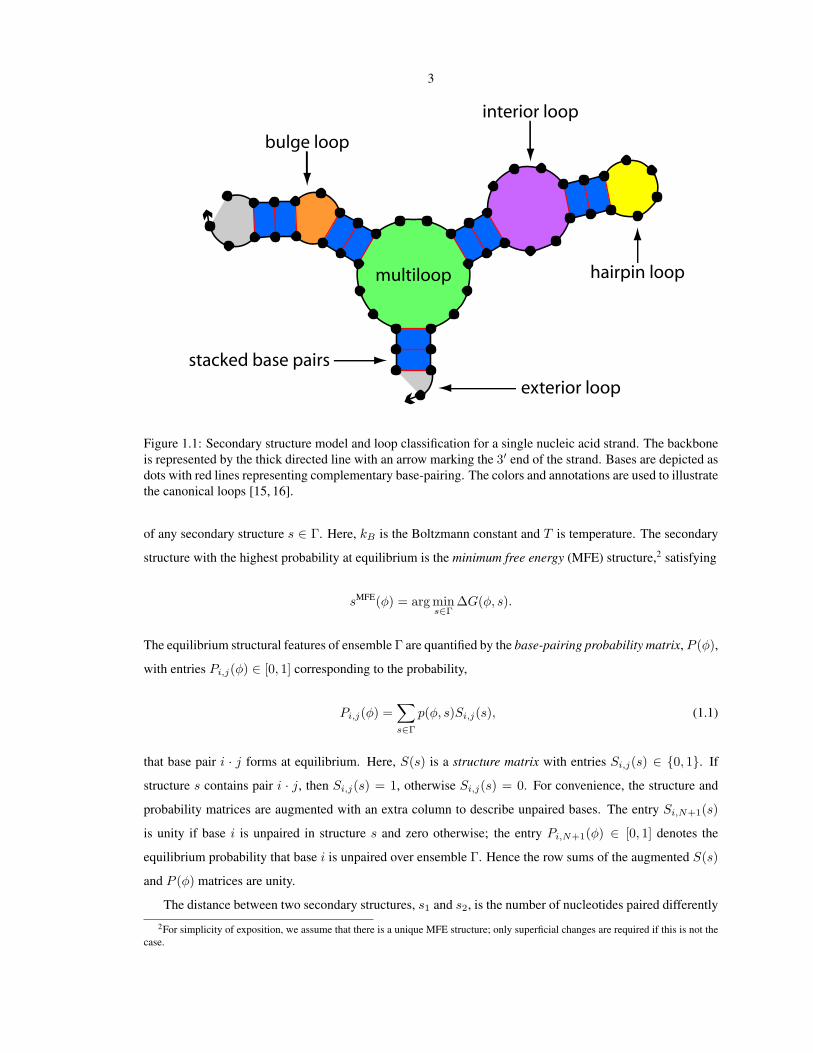
classification is depicted in Figure 1.1. This physical model provides the basis for rigorous analysis and
design of equilibrium base-pairing in the context of the free energy landscape defined over ensemble Γ.
1.1.2 Characterizing equilibrium secondary structure
By calculating the partition function [17],
Q(φ) =∑s∈Γ
e−∆G(φ,s)/kBT ,
over Γ, it is possible to evaluate the equilibrium probability,
p(φ, s) =1
Q(φ)e−∆G(φ,s)/kBT ,
1Pseudoknotted structures are excluded from the ensemble Γ for computational expediency.
3
hairpin loop
interior loop
bulge loop
stacked base pairs
exterior loop
multiloop
Figure 1.1: Secondary structure model and loop classification for a single nucleic acid strand. The backboneis represented by the thick directed line with an arrow marking the 3′ end of the strand. Bases are depicted asdots with red lines representing complementary base-pairing. The colors and annotations are used to illustratethe canonical loops [15, 16].
of any secondary structure s ∈ Γ. Here, kB is the Boltzmann constant and T is temperature. The secondary
structure with the highest probability at equilibrium is the minimum free energy (MFE) structure,2 satisfying
sMFE(φ) = arg mins∈Γ
∆G(φ, s).
The equilibrium structural features of ensemble Γ are quantified by the base-pairing probability matrix, P (φ),
with entries Pi,j(φ) ∈ [0, 1] corresponding to the probability,
Pi,j(φ) =∑s∈Γ
p(φ, s)Si,j(s), (1.1)
that base pair i · j forms at equilibrium. Here, S(s) is a structure matrix with entries Si,j(s) ∈ 0, 1. If
structure s contains pair i · j, then Si,j(s) = 1, otherwise Si,j(s) = 0. For convenience, the structure and
probability matrices are augmented with an extra column to describe unpaired bases. The entry Si,N+1(s)
is unity if base i is unpaired in structure s and zero otherwise; the entry Pi,N+1(φ) ∈ [0, 1] denotes the
equilibrium probability that base i is unpaired over ensemble Γ. Hence the row sums of the augmented S(s)
and P (φ) matrices are unity.
The distance between two secondary structures, s1 and s2, is the number of nucleotides paired differently
2For simplicity of exposition, we assume that there is a unique MFE structure; only superficial changes are required if this is not thecase.

4
in the two structures:
d(s1, s2) = N −∑
1 ≤ i ≤ N
1 ≤ j ≤ N+1
Si,j(s1)Si,j(s2).
We also define the discrete delta function
δs1,s2 =
1, if d(s1, s2) = 0,
0, otherwise,
with respect to secondary structure.
Although the size of the ensemble, Γ, grows exponentially with the number of nucleotides N [18], the
MFE structure, the partition function, and the equilibrium base-pairing probabilities can all be calculated via
Θ(N3) dynamic programs [8, 18–25].These dynamic programming algorithms can also be parallelized with
their efficiency to run on multiple computational cores [20, 26].
1.2 Thermodynamic sequence design
For a given target structure, s, we formulate sequence design as an optimization problem, minimizing an
objective function with respect to sequence, φ. Rather than seeking a global optimum, we terminate opti-
mization if the objective function is reduced below a prescribed stop condition.
1.2.1 Objective functions
MFE defect optimization
One strategy is to minimize the MFE defect [20, 27–30]:
µ(φ, s) = d(sMFE, s)
= N −∑
1 ≤ i ≤ N
1 ≤ j ≤ N+1
Si,j(sMFE(φ))Si,j(s),
corresponding to the distance between the MFE structure sMFE(φ) and the target structure s. The util-
ity of this approach hinges on whether or not the equilibrium structural features of ensemble Γ are well-
characterized by the single structure sMFE(φ), which in turn depends on the specific sequence φ [31]. If
µ(φ, s) = 0, the target structure s is the most probable secondary structure at equilibrium; p(φ, s) can
nonetheless be arbitrarily small due to competition from other secondary structures in Γ.

5
Probability defect optimization
To address this concern, an alternative strategy is to minimize the probability defect [20, 31, 32]:
π(φ, s) = 1− p(φ, s),
corresponding to the sum of the probabilities of all non-target structures in the ensemble Γ. If π(φ, s) ≈
0, the sequence design is essentially ideal because the equilibrium structural properties of the ensemble
are dominated by the target structure s. However, as π(φ, s) deviates from zero, it increasingly fails to
characterize the quality of the sequence because the probability defect treats all non-target structures as being
equally defective. This property is a concern for challenging designs where it may be infeasible to achieve
π(φ, s) ≈ 0.
Ensemble defect optimization
To address these shortcomings, a third strategy minimizes the ensemble defect [31]:
n(φ, s) =∑σ∈Γ
p(φ, σ)d(σ, s) (1.2)
= N −∑
1 ≤ i ≤ N
1 ≤ j ≤ N+1
Pi,j(φ)Si,j(s), (1.3)
corresponding to the average number of incorrectly paired nucleotides at equilibrium calculated over ensem-
ble Γ.
Comparing formulations
We cast these three objective functions into a unified formulation to highlight their differences:
n(φ, s) =∑σ∈Γ
p(φ, σ)d(σ, s),
µ(φ, s) =∑σ∈Γ
δσ,sMFEd(σ, s),
π(φ, s) =∑σ∈Γ
p(φ, σ)(1− δσ,s).
Using n(φ, s) to perform ensemble optimization, the average number of incorrectly paired nucleotides at
equilibrium is evaluated over ensemble Γ using p(φ, σ), the Boltzmann-weighted probability of each sec-
ondary structure σ ∈ Γ, and d(σ, s), the distance between each secondary structure σ ∈ Γ and the target
structure s. By comparison, using µ(φ, s) to perform MFE defect optimization, p(φ, σ) is replaced by the

6
discrete delta function δσ,sMFE , which is unity for sMFE and zero for all other structures σ ∈ Γ. Alternatively,
using π(φ, s) to perform probability defect optimization, d(σ, s) is replaced by the binary distance function
(1− δσ,s) that is zero for s and 1 for all other structures σ ∈ Γ. Hence, the MFE defect makes the optimistic
assumption that sMFE will dominate Γ at equilibrium, while the probability defect makes the pessimistic
assumption that all structures σ ∈ Γ with d(σ, s) 6= 0 are equally distant from the target structure s. The
objective function n(φ, s) quantifies the equilibrium structural defects of sequence φ even when µ(φ, s) and
π(φ, s) do not.
1.2.2 Prior optimization algorithms
The computational challenge of rational sequence design stems from sequence space growing exponentially
with the linear size of the desired target structure. One approach is to employ a local search strategy inspired
by biological evolution to optimize a thermodynamic objective function. These randomized algorithms ex-
plore local neighbors by mutating the identity of a base or base pair followed by an objective function eval-
uation. If the mutation lowered the value of the objective function, the mutation is saved, otherwise it is
accepted with a probability less than one [20, 27, 28, 31–34].
Previous implementations of probability defect optimization [20, 31–33] and ensemble optimization [31]
employed single-scale mutation procedures in which each candidate mutation was evaluated on the full se-
quence using Θ(N3) dynamic programs to calculate Q(φ) or P (φ), respectively. By comparison, more effi-
cient hierarchical mutation procedures have been developed for MFE defect optimization [20, 27, 28]. These
methods perform a hierarchical decomposition of the target structure, optimizing subsequences on a series
of growing substructures to reduce the number of times that sMFE(φ) is calculated on the full sequence using
a Θ(N3) dynamic program. Furthermore, to reduce the total number of mutations that must be evaluated,
these methods guide the selection of candidate mutation positions based on defects in the MFE substructure
[20, 27, 28].
1.3 Thesis outline
Here, we develop an ensemble defect optimization algorithm that employs hierarchical decomposition and
weighted mutation sampling to simultaneously achieve high design quality and low design cost. We then
expand this algorithm to achieve high-quality, low cost ensemble defect optimization for linked multi-state
nucleic acid systems, thus increasing the versatility of nucleic acid design. In order to improve the accessibil-
ity and ease of use of these algorithms, we describe a web application for the design and analysis of nucleic
acid systems.
In Chapter 2 we describe the single-complex design algorithm and perform computational studies that
characterize the algorithmic ingredients and compare performance to previous design approaches. We also
make empirical observations about the algorithm’s running time with respect to the theoretical lower bound.

7
Motivated by these results and previous invented multi-state nucleic acid systems, in Chapter 3 we improve
the versatility of this algorithm to achieve high-quality designs of multiple linked targets at a reduced cost.
Finally, in Chapter 4, we describe the NUPACK web server for the analysis and design of nucleic acid
systems, as a means for researchers to design, analyze, and visualize nucleic acids.

8
Chapter 2
Nucleic acid sequence design via efficientensemble defect optimization
The work in this chapter is based on the following submitted manuscript: J. N. Zadeh, B. R. Wolfe, and N.
A. Pierce. Nucleic acid sequence design via efficient ensemble defect optimization.
2.1 Introduction
Here, we describe a sequence design algorithm that achieves high design quality via ensemble defect opti-
mization, and low design cost via hierarchical structure decomposition and defect-weighted sampling. For
a given target secondary structure, s, with N nucleotides, we seek to design a sequence, φ, with ensemble
defect, n(φ, s), satisfying the stop condition:
n(φ, s) ≤ fstopN,
for a user-specified value of fstop ∈ (0, 1). Candidate mutations are evaluated at the leaves of a binary tree
decomposition of the target structure. During leaf optimization, defect-weighted mutation sampling is used
to select each candidate mutation position with probability proportional to its contribution to the ensemble
defect of the leaf. If emergent structural defects are encountered when merging subsequences moving up the
tree, they are eliminated via defect-weighted child sampling and reoptimization. This design algorithm is
outlined below and detailed in the pseudocode of Algorithm 2.1.
2.2 Algorithm description
2.2.1 Hierarchical structure decomposition
Prior to sequence design, the target structure s is decomposed into a (possibly unbalanced) binary tree of
substructures, with each node of the tree indexed by a unique integer k. For each parent node, k, there is a left
9
child node, kl, and a right child node, kr. Each nucleotide in parent structure sk is partitioned to either the
left or right child substructure (sk = skl ∪ skr and skl ∩ skr = ∅). Child node kl inherits from parent node k the
augmented substructure, skl+, comprising native nucleotides, skl
native ≡ skl , and additional dummy nucleotides
that approximate the influence of its sibling in the context of their parent (skl ≡ skl
native ∪ skl
dummy ≡ skl+).
In contrast to earlier hierarchical methods that decompose parent structures at multiloops [20, 27], our
algorithm decomposes parent structures within duplex stems. This approach is more generally applicable
to the design of duplex-rich engineered structures that often contain no multiloops. Eligible split-points are
those locations within a duplex stem with at least Hsplit consecutive base-pairs to either side, such that both
children would have at least Nsplit nucleotides. If there are no eligible split-points, a structure becomes a leaf
node in the decomposition tree. Otherwise, an eligible split-point is selected so as to minimize the difference
in the size of the children, ||skl | − |skr ||. Dummy nucleotides are defined by extending the newly-split duplex
stem across the split-point by Hsplit base pairs (|skl
dummy| = 2Hsplit).
For a parent node k, the sequence φk follows the same partitioning as the structure sk (φk = φkl ∪ φkrand φkl ∩ φkr = ∅). Likewise, for a child node kl, the sequence contains both native and dummy nucleotides
(φkl ≡ φkl
native ∪ φkl
dummy ≡ φkl+).
For any node k with sequence φk and structure sk, the ensemble defect, nk ≡ n(φk, sk), may be ex-
pressed as
nk =∑
1≤i≤|sk|
nki ,
where
nki = 1−∑
1≤j≤|sk|+1
P ki,jSki,j .
is the contribution of nucleotide i to the ensemble defect of the node. For a parent node k, the ensemble defect
can be expressed as a sum of contributions from bases partitioned to the left and right children (nk = nkl +nkr ).
For a child node kl, the ensemble defect can be expressed as a sum of contributions from native and dummy
nucleotides (nkl = nkl
native +nkl
dummy). Conceptually, nkl
native, the contribution of the native nucleotides to the
ensemble defect of child kl (calculated on child node kl at cost Θ(|skl |3), approximates nkl , the contribution
of the left-child nucleotides to the ensemble defect of parent k (calculated on parent node k at higher cost
Θ(|sk|3)). In general, nkl
native 6= nkl , because the dummy nucleotides in child node kl only approximate the
influence of its sibling (which is fully accounted for only in the more expensive calculation on parent node
k).
The utility of hierarchical structure decomposition hinges on the assumption that sequence space is suf-
ficiently rich that two subsequences optimized for sibling substructures will often not exhibit crosstalk when
merged by a parent node. Our hierarchical mutation procedure is designed to benefit from this property when
it holds true, and to eliminate emergent defects when they do arise.

10
2.2.2 Leaf optimization with weighted mutation sampling
The sequence design process is initialized by randomly specifying the identities of all nucleotides in the
leaf structures, subject to the constraint that bases intended to be paired are chosen to be Watson-Crick
complements. At leaf node k, sequence optimization is performed by mutating either one base at a time (if
Ski,|sk|+1 = 1) or one base pair at a time (if Ski,j = 1 for some 1 ≤ j ≤ |sk|, in which case φki and φkj are
mutated simultaneously so as to remain Watson-Crick complements).
We perform defect-weighted mutation sampling by selecting nucleotide i as a candidate for mutation with
probability nki /nk. A candidate sequence φk is evaluated via calculation of nk if the candidate mutation, ξ, is
not in the set of previously rejected mutations, γunfavorable (position and sequence). A candidate mutation is
retained if nk < nk and rejected otherwise. The set, γunfavorable, is updated after each unsuccessful mutation
and cleared after each successful mutation.
Optimization of leaf k terminates successfully if the leaf stop condition:
nk ≤ fstop|sk|
is satisfied, or restarts ifMunfavorable|sk| consecutive unfavorable candidate mutations are either in γunfavorable
or are evaluated and added to γunfavorable. Leaf optimization is attempted from new random initial conditions
up toMleafopt times before terminating unsuccessfully. The outcome of leaf optimization is the leaf sequence
φk corresponding to the lowest encountered value of the leaf ensemble defect nk.
2.2.3 Subsequence merging and reoptimization
After sibling nodes kl and kr have been optimized, parent node k merges their native subsequences (setting
φkl = φkl
native and φkr = φkr
native) and evaluates nk to check the parental stop condition:
nk ≤ max(fstop|skl |, nkl
native) + max(fstop|skr |, nkr
native).
If this stop condition is satisfied, subsequence merging continues up the tree. Otherwise, failure to satisfy
the stop condition implies the existence of emergent defects resulting from crosstalk between the two child
sequences. In this case, parent node k initiates defect-weighted child sampling and reoptimization within its
subtree. Left child kl is selected for reoptimization with probability nkl /nk and right child kr is selected
for reoptimization with probability nkr/nk. This defect-weighted child sampling procedure is performed
recursively until a leaf is encountered (each time using partitioned defect information inherited from the
parent k that initiated the reoptimization). The standard leaf optimization procedure is then performed starting
from a new random initial sequence. The use of random initial conditions during leaf reoptimization is based
on the assumption that sequence space is sufficiently rich that emergent defects can typically be eliminated
simply by designing a different leaf sequence. Following leaf reoptimization, merging begins again starting
11
with the reoptimized leaf and its sibling. The elimination of emergent defects in parent k by defect-weighted
child sampling and reoptimization is attempted up to Mreopt times.
2.2.4 Optimality bound and time complexity
This hierarchical sequence design approach implies an asymptotic optimality bound on the cost of designing
the full sequence relative to the cost of evaluating a single candidate mutation on the full sequence. For
a target structure with N nucleotides, evaluation of a candidate sequence requires calculation of n(φ, s) at
cost ceval(N) = Θ(N3). Performing sequence design using hierarchical structure decomposition, mutations
are evaluated at the leaf nodes and merged subsequences are evaluated at all other nodes. For node k, the
evaluation cost is ceval(|sk|). If at least one mutation is required in each leaf, the design cost is minimized by
maximizing the depth of the binary tree. Furthermore, at each depth in the tree, the design cost is minimized
by balancing the tree. Hence, a lower bound on the cost of designing the full sequence is given by
cdes(N) ≥ ceval(N)[1 + 2
(12
)3 + 4(
14
)3 + 8(
18
)3 + . . .]
or
cdes(N) ≥ 43ceval(N).
Hence, if the sequence design algorithm performs optimally for large N , we would expect the cost of full
sequence design to be 4/3 the cost of evaluating a single mutation on the full sequence. In practice, many
factors might be expected to undermine optimality: imperfect balancing of the tree, the addition of dummy
nucleotides in each non-root node, the use of finite tree depth, leaf optimizations requiring evaluation of mul-
tiple candidate mutations, and reoptimization to eliminate emergent defects. This optimality bound implies
time complexity Ω(N3) for the sequence design algorithm.
2.3 Methods
Computational sequence design studies were performed using the default algorithm parameters of Table 2.1.
Design trials were run on a cluster of 2.53 GHz Intel E5540 Xeon dual-processor/quad-core nodes with 24
GB of memory per node.
2.3.1 Structure test sets
Algorithm performance was evaluated on structure test sets containing 30 target structures for each of N ∈
100, 200, 400, 800, 1600, 3200. An engineered test set was generated by randomly selecting structural
components and dimensions from ranges intended to reflect current practice in engineering nucleic acid
secondary structures. A multi-stranded version was produced by introducing nicks into the structures in

12
DESIGNSEQ(φ, s, n, k)a← DEPTH(k)if HASCHILDREN(k)
mreopt ← 0if n = ∅
φl ← DESIGNSEQ(∅, sl+, ∅, kl)φr ← DESIGNSEQ(∅, sr+, ∅, kr)
elseUPDATECHILDREN(k, a, a− 1)child, φ← WEIGHTEDCHILDSAMPLING(φ, s, nl, nr)φchild ← DESIGNSEQ(φchild+, schild+, nchild+, kchild)
nk,a ← ENSEMBLEDEFECT(φ, s)UPDATECHILDREN(k, a, a+ 1)
while nk,a > max(fstop|sl|, nkl,a
native) + max(fstop|sr|, nkr,anative)
andmreopt < Mreopt
child, φ← WEIGHTEDCHILDSAMPLING(φ, s, nk,al , nk,a
r )
φchild ← DESIGNSEQ(φchild+, schild+, nk,achild+, kchild)
n← ENSEMBLEDEFECT(φ, s)
if n < nk,a
φ, nk,a ← φ, nUPDATECHILDREN(k, a, a+ 1)
mreopt ← mreopt + 1else
mleafopt ← 0
φ, nk,a ← OPTIMIZELEAF(s)
while nk,a > fstop|s| andmleafopt < Mleafopt
φ, n← OPTIMIZELEAF(s)
if n < nk,a
φ, nk,a ← φ, nmleafopt ← mleafopt + 1
return φnative
UPDATECHILDREN(k, a, b)
if HASCHILDREN(k)
nkl,a ← nkl,b
nkr,a ← nkr,b
UPDATECHILDREN(kl, a, b)UPDATECHILDREN(kr, a, b)
OPTIMIZELEAF(s)
munfavorable ← 0γunfavorable ← ∅φ← INITSEQ(s)n← ENSEMBLEDEFECT(φ, s)while n > fstop|s| andmunfavorable < Munfavorable|s|
ξ, φ← WEIGHTEDMUTATIONSAMPLING(φ, s, n1, . . . , n|s|)if ξ ∈ γunfavorable
munfavorable ← munfavorable + 1else
n← ENSEMBLEDEFECT(φ, s)if n < n
φ, n← φ, nmunfavorable ← 0γunfavorable ← ∅
elsemunfavorable ← munfavorable + 1γunfavorable ← γunfavorable∪ ξ
return φ, n
Algorithm 2.1: Pseudocode for hierarchical ensemble defect optimization with defect-weighted sampling.For a given target structure s, a designed sequence φ is returned by the function call DESIGNSEQ(∅, s, ∅, 1).During the recursive design procedure, φ, s, and n are local variables that are used to push sequence, structure,and defect information between nodes in the tree. By contrast, nk,a provides global storage for the ensembledefect of each node k. For a given k, the index, a = 1, . . . ,DEPTH(k), enables storage of the ensemble defectcorresponding to the sequence for node k that has been accepted up to depth a in the tree. Storage of thesehistorical values eliminates unnecessary recalculation of ensemble defects during subtree reoptimization.

13
the engineered test set. Each structure in a random test set was obtained by calculating an MFE structure of
a different random RNA sequence at 37C. Figure 2.1 compares the structural features of the engineered and
random test sets. In general, the random test set has target structures with a lower fraction of bases paired,
more duplex stems, and shorter duplex stems (as short as one base pair). Additional structural features of
the engineered and random test sets are summarized in Appendix B, Figure B.1. For the design studies that
follow, new target structure test sets were generated from scratch. The design algorithm was not tested on
these structures prior to generating the depicted results.
EngineeredRandom
40Base pairs per stem
0 8 16 24 32
Num
ber o
f ste
ms
0
2000
3000c
1000
300Stems per structure
0 60 120 180 240
Num
ber o
f stru
cture
s
0
5
10
15b
Num
ber o
f stru
cture
s
0.0 0.2 0.4 0.6 0.8 1.00
40
80
120
Fraction of bases paired
a
Figure 2.1: Comparison of the structural features of the engineered and random test sets.
2.3.2 Other algorithms
To illustrate the roles of hierarchical structure decomposition and weighted mutation sampling in the context
of ensemble optimization, we compare our algorithm to three alternative algorithms lacking either or both of
these features:
• Single-scale ensemble defect optimization with uniform mutation sampling [31]. The leaf optimization
algorithm is applied directly on the full sequence using uniform mutation sampling in which each can-
didate mutation position is selected with equal probability (pseudocode in Appendix C, Algorithm C.1).
• Single-scale ensemble defect optimization with defect-weighted mutation sampling. The leaf optimiza-
tion algorithm is applied directly on the full sequence (pseudocode in Appendix C, Algorithm C.2).
• Hierarchical ensemble defect optimization with uniform mutation sampling. The hierarchical algorithm
is applied using uniform mutation sampling during leaf optimization and uniform child sampling during
Parameter ValueHsplit 2Nsplit 20fstop 0.01Mreopt 10Mleafopt 3Munfavorable 4
Table 2.1: Default parameter values used in evaluating algorithm performance for RNA design. For DNAdesign, Hsplit = 3.
14
subsequence merging and reoptimization (pseudocode in Appendix C, Algorithm C.3).
We also modified our algorithm to compare performance to algorithms inspired by previous work:
• Single-scale probability defect optimization with uniform mutation sampling [20, 31–33]. This method
seeks to design a sequence such that the probability defect satisfies the stop condition π(φ, s) ≤ fstop.
Satisfaction of this stop condition is sufficient to ensure that stop conditions n(φ, s) ≤ fstopN and
µ(φ, s) ≤ fstopN are also satisfied for fstop ∈ (0, 0.5]. Optimization is performed using a modified
version of the leaf optimization algorithm (with π(φ, s) taking the role of n(φ, s)) applied directly on
the full sequence using uniform mutation sampling (pseudocode in Appendix C, Algorithm C.4).
• Hierarchical MFE defect optimization with weighted mutation sampling [20, 27, 28]. This method
seeks to design a sequence such that the MFE defect satisfies the stop condition µ(φ, s) ≤ fstopN .
Optimization is performed using a modified version of our algorithm with µk taking the role of nk
(pseudocode in Appendix C Algorithm C.5).
2.3.3 Implementation
The sequence design algorithm is coded in the C programming language. By parallelizing the dynamic
program for evaluating P (φ) using MPI [26], the sequence design algorithm can also reduce run time using
multiple cores. For a design job allocated M computational cores, each evaluation of P k for node k with
structure sk is performed using m cores for some m ∈ 1, ...,M selected to approximately minimize run time
based on |sk| [35]). More implementation and infrastructure details are given in Appendix A.
2.4 Computational design studies
Our primary test scenario is RNA sequence design at 37C for target structures in the engineered test set.
For each target structure in a test set, 10 independent design trials were performed. Each plotted data point
represents a median over 300 design trials (10 trials for each of 30 structures for a given size N ).
2.4.1 Algorithm performance and asymptotic optimality
Figure 2.2 demonstrates the typical performance of our algorithm across a range of values of N using the
engineered and random test sets. Typical designs surpass the desired design quality (n(φ, s) ≤ N/100) as a
result of overshooting stop conditions lower in the decomposition tree (panel a). For the engineered test set,
typical design cost ranges from a fraction of a second for N = 100 to roughly three hours for N = 3200
(panel b). For small N , the design cost for the random test set is higher than for the engineered test set,
becoming comparable as N increases. Typical GC content is less than 60% (starting from random initial
sequences with ≈50% GC content; panel c). Remarkably, as the depth of the decomposition tree increases

15
102 103
0.005
0.01
Design Quality
Target structure size N (nt)
Norm
alize
d en
sem
ble d
efec
tn(!,s
)/N
stop condition
102 10310!1
100
101
102
103
104
Design Cost
Target structure size N (nt)
Wall
cloc
k tim
e (s
)
102 1030.4
0.5
0.6
0.7
0.8
Target structure size N (nt)
GC co
nten
t
Sequence Composition
initial condition
102 10315
1015202530
c des(N
) / c ev
al(N)
Target structure size N (nt)
Relative Design Cost
Engineered test setRandom test set
optimality bound
a b
dc
Figure 2.2: Algorithm performance and asymptotic optimality. a) Design quality. The stop condition isdepicted as a dashed line. b) Design cost. c) Sequence composition. The initial GC content is depictedas a dashed line. d) Cost of sequence design relative to a single evaluation of the objective function. Theoptimality bound is depicted as a dashed line. RNA design at 37C on the engineered and random test sets.
with N , the relative cost of design, cdes(N)/ceval(N), decreases asymptotically to the optimal bound of 4/3
(panel d). Hence, for sufficiently large N , the typical cost of sequence design is only 4/3 the cost of a single
mutation evaluation on the root node. Mutation evaluation has time complexity Θ(N3) and is empirically
observed to be approximately in the asymptotic regime (Figure 2.3). Hence, for our design algorithm, the
empirical observation of asymptotic optimality implies that the exponent in the Ω(N3) time complexity
bound is sharp.
2.4.2 Leaf independence and emergent defects
Figure 2.4 compares the ensemble defect evaluated at the root node, to the sum of the ensemble defects
evaluated at the leaf nodes.1 If the assumption of leaf independence is valid (i.e., if dummy nucleotides do a
good job of mimicking parental environments and there is minimal crosstalk between merged subsequences),
we would expect the data to fall near the diagonal.
For the engineered test set (panel a), we observe three striking properties. First, for random initial se-
quences, the assumption of leaf independence is well-justified despite the fact that the ensemble defect is
large. Second, leaf optimization followed by merging without reoptimization (i.e., Mreopt = 0) typically
1To avoid overcounting defects at the leaves, nki is counted in leaf k only if nucleotide i is native throughout its ancestry.

16
102 103
10!1100101102103104105
Wall
cloc
k tim
e (s
)Target structure size N (nt)
Evaluation Cost
Figure 2.3: Computational cost, ceval(N) = Θ(N3), of a single evaluation of the ensemble defect, n(φ, s),for the full sequence and target structure. Each data point represents the median over all sequences for aparticular value of N . The line depicts a slope of three, suggesting empirically that the dynamic programis operating approximately within the asymptotic regime for this range of N . RNA design at 37C on theengineered test set.
10!3 10!2 10!1 10010!3
10!2
10!1
100
[Sum of leaf n(!,s)]/N
Root
n(!
,s)/N
Random sequencesLeaf!optimized sequencesFinal sequence designs
10!3 10!2 10!1 10010!3
10!2
10!1
100
[Sum of leaf n(!,s)]/N
Root
n(!
,s)/N
a b
Figure 2.4: Leaf independence and emergent defects. Comparison of the ensemble defect evaluated atthe root node to the sum of the ensemble defects evaluated at the leaf nodes. a) Engineered test set.b) Random test set. Dots represent independent designs. Symbols denote medians for each value ofN ∈ 100, 200, 400, 800, 1600, 3200 (symbol size increases with N ). RNA design at 37C.
17
yields full sequence designs that achieve the desired design quality (n(φ, s) ≤ N/100 on the root), with
emergent defects arising only in a minority of cases. Third, these emergent defects are successfully elimi-
nated by defect-weighted child sampling and reoptimization starting from new random initial subsequences.
The resulting full sequence designs exhibit leaf independence and satisfy the stop condition.
By comparison, for the random test set, merging of leaf-optimized sequences typically does lead to emer-
gent defects in the root node. Even in this case, our algorithm successfully eliminates emergent defects using
defect-weighted child sampling and reoptimization starting from new random initial subsequences.
2.4.3 Contributions of algorithmic ingredients
Figure 2.5 isolates the contributions of hierarchical structure decomposition and defect-weighted sampling to
our ensemble defect optimization algorithm by comparing performance to three modified algorithms lacking
one or both ingredients. All four methods typically achieve the desired design quality, with hierarchical
methods surpassing the quality requirement for the root node as a result of overshooting stop conditions
lower in the decomposition tree. Hierarchical methods dramatically reduce design cost relative to their single-
scale counterparts (which are not tested for N = 800 due to high cost). Defect-weighted sampling reduces
design cost and GC content by focusing mutation effort on the most defective subsequences. For the single-
scale methods, the relative cost of design, cdes(N)/ceval(N), increases with N . For hierarchical methods,
cdes(N)/ceval(N) decreases asymptotically to the optimal bound of 4/3 as N increases. Our algorithm thus
combines the design quality of ensemble defect optimization, the reduced cost and asymptotic optimality of
hierarchical decomposition, and the reduced cost and reduced GC content of defect-weighted sampling.
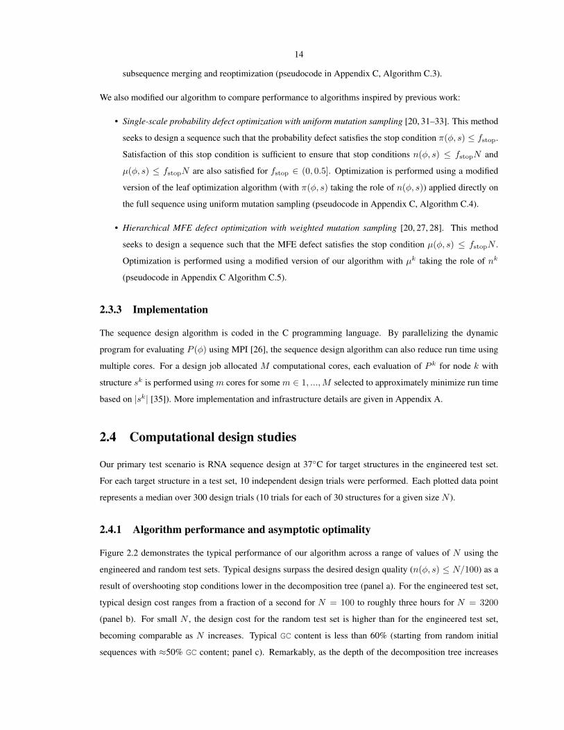
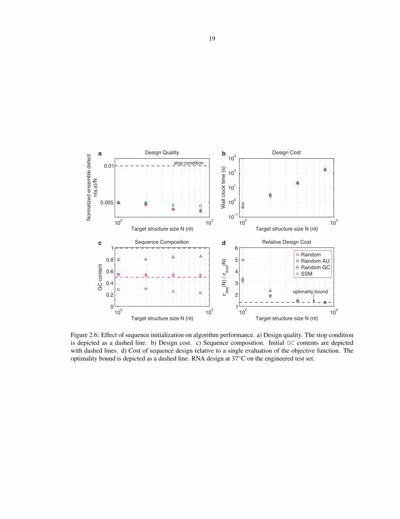
2.4.4 Sequence initialization
To explore the effect of sequence initialization on typical design quality and cost, we tested four types of initial
conditions (Figure 2.6): random sequences (default), random sequences using only A and T bases, random
sequences using only G and C bases, and sequences satisfying sequence symmetry minimization (SSM) [3].2
The desired design quality is achieved independent of the initial conditions (panel a), which have little effect
on design cost (panels b and d). Designs initiated with random AT sequences or with random GC sequences
illustrate that the ensemble defect stop condition can be satisfied over a broad range of GC contents (panel c).
2.4.5 Stop condition stringency
Figure 2.7 depicts typical algorithm performance for five different levels of stringency in the stop condition:
fstop ∈ 0.001, 0.005, 0.01(default), 0.05, 0.10. For each stop condition, the observed design quality is
better than required (resulting from overshooting stop conditions lower in the decomposition tree). Consistent
2SSM is a heuristic that promotes specificity for the target structure by prohibiting repeated subsequences of a specified word length(taken to be six for our tests). For bases in single-stranded or branched regions of the target structure, the complementary word is alsoprohibited[3].

18
102 103
0.005
0.01
Design Quality
Target structure size N (nt)
Norm
alize
d en
sem
ble d
efec
tn(!,s
)/N
stop condition
102 10310!1100101102103104105 Design Cost
Target structure size N (nt)
Wall
cloc
k tim
e (s
)
102 1030.4
0.5
0.6
0.7
0.8
Target structure size N (nt)
GC co
nten
t
Sequence Composition
initial condition
102 103100
101
102
103c de
s(N) /
c eval(N
)
Target structure size N (nt)
Relative Design Cost
Uniform samplingDefect-weighted sampling
Uniform samplingDefect-weighted sampling
optimality bound
Single-scale optimization Hierarchical optimization
a b
dc
Figure 2.5: Contributions of hierarchical structure decomposition and defect-weighted sampling to algorithmperformance. a) Design quality. The stop condition is depicted as a dashed line. b) Design cost. c) Sequencecomposition. The initial GC content is depicted as a dashed line. d) Cost of sequence design relative to asingle evaluation of the objective function. The optimality bound is depicted as a dashed line. RNA design at37C on the engineered test set.
19
102 103
0.005
0.01
Design Quality
Target structure size N (nt)
Norm
alize
d en
sem
ble d
efec
tn(!,s
)/N
stop condition
102 10310!1
100
101
102
103 Design Cost
Target structure size N (nt)W
all cl
ock t
ime
(s)
102 1030
0.2
0.4
0.6
0.8
1
Target structure size N (nt)
GC co
nten
t
Sequence Composition
102 1031
2
3
4
5
6
c des(N
) / c ev
al(N)
Target structure size N (nt)
Relative Design Cost
RandomRandom AURandom GCSSM
optimality bound
a b
dc
Figure 2.6: Effect of sequence initialization on algorithm performance. a) Design quality. The stop conditionis depicted as a dashed line. b) Design cost. c) Sequence composition. Initial GC contents are depictedwith dashed lines. d) Cost of sequence design relative to a single evaluation of the objective function. Theoptimality bound is depicted as a dashed line. RNA design at 37C on the engineered test set.

20
102 10310!4
Design Quality
Target structure size N (nt)
Norm
alize
d en
sem
ble d
efec
tn(!,s
)/N
102 10310!1
100
101
102
103 Design Cost
Target structure size N (nt)
Wall
cloc
k tim
e (s
)102 1030.4
0.5
0.6
0.7
0.8
Target structure size N (nt)
GC co
nten
t
Sequence Composition
initial condition
102 1031
10
20
30
c des(N
) / c ev
al(N)
Target structure size N (nt)
Relative Design Cost
fstop = 0.001fstop = 0.005fstop = 0.01fstop = 0.05fstop = 0.1
optimality bound
10!3
10!1
10!2
a b
dc
Figure 2.7: Effect of stop condition stringency on algorithm performance. a) Design quality. Stop conditionsare depicted by dashed lines. b) Design cost. c) Sequence composition. The initial GC content is depictedas a dashed line. d) Cost of sequence design relative to a single evaluation of the objective function. Theoptimality bound is depicted as a dashed line. RNA design at 37C on the engineered test set.
with empirical asymptotic optimality, the design cost is independent of fstop for sufficiently large N (for the
tested stringency levels). It is noteworthy that the algorithm is capable of routinely and efficiently designing
sequences with ensemble defect less than N/1000.
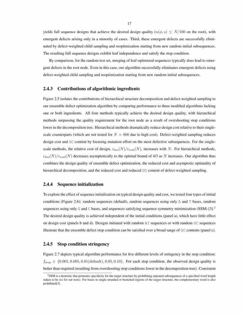
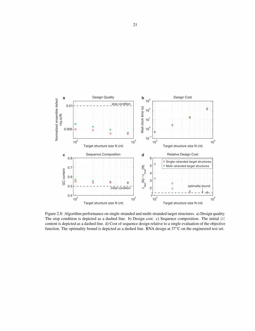
2.4.6 Multi-stranded target structures
Multi-stranded target structures arise frequently in engineering practice [4, 5, 7]. Figure 2.8 demonstrates that
our algorithm performs similarly on single-stranded and multi-stranded target structures.
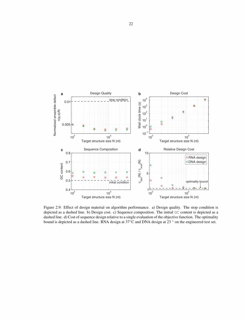
2.4.7 Design material
Figure 2.9 compares RNA and DNA design. DNA designs are performed in 1 M Na+ at 23 C to reflect that
DNA systems are typically engineered for room temperature studies. In comparison to RNA design, DNA
design leads to similar design quality (panel a), higher design cost (panel b), and somewhat higher GC content
(panel c), while continuing to exhibit asymptotic optimality (panel d).
21
102 103
0.005
0.01
Design Quality
Target structure size N (nt)
Norm
alize
d en
sem
ble d
efec
tn(!,s
)/N
stop condition
102 10310!1
100
101
102
103 Design Cost
Target structure size N (nt)W
all cl
ock t
ime
(s)
102 1030.4
0.5
0.6
0.7
0.8
Target structure size N (nt)
GC co
nten
t
Sequence Composition
initial condition
102 1031
2
3
4
5
6
c des(N
) / c ev
al(N)
Target structure size N (nt)
Relative Design Cost
Single!stranded target structuresMulti!stranded target structures
optimality bound
a b
dc
Figure 2.8: Algorithm performance on single-stranded and multi-stranded target structures. a) Design quality.The stop condition is depicted as a dashed line. b) Design cost. c) Sequence composition. The initial GCcontent is depicted as a dashed line. d) Cost of sequence design relative to a single evaluation of the objectivefunction. The optimality bound is depicted as a dashed line. RNA design at 37C on the engineered test set.
22
102 103
0.005
0.01
Design Quality
Target structure size N (nt)
Norm
alize
d en
sem
ble d
efec
tn(!,s
)/N
stop condition
102 10310!1
100
101
102
103
104
Design Cost
Target structure size N (nt)W
all cl
ock t
ime
(s)
102 1030.4
0.5
0.6
0.7
0.8
Target structure size N (nt)
GC co
nten
t
Sequence Composition
initial condition
102 1031
5
10
c des(N
) / c ev
al(N)
Target structure size N (nt)
Relative Design Cost
RNA designDNA design
optimality bound
a b
dc
Figure 2.9: Effect of design material on algorithm performance. a) Design quality. The stop condition isdepicted as a dashed line. b) Design cost. c) Sequence composition. The initial GC content is depicted as adashed line. d) Cost of sequence design relative to a single evaluation of the objective function. The optimalitybound is depicted as a dashed line. RNA design at 37C and DNA design at 23 on the engineered test set.
23
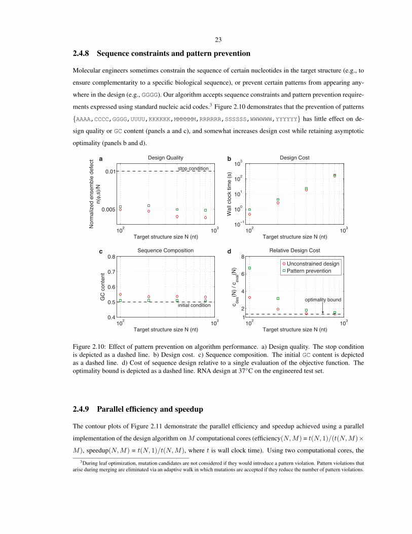
2.4.8 Sequence constraints and pattern prevention
Molecular engineers sometimes constrain the sequence of certain nucleotides in the target structure (e.g., to
ensure complementarity to a specific biological sequence), or prevent certain patterns from appearing any-
where in the design (e.g., GGGG). Our algorithm accepts sequence constraints and pattern prevention require-
ments expressed using standard nucleic acid codes.3 Figure 2.10 demonstrates that the prevention of patterns
AAAA,CCCC,GGGG,UUUU,KKKKKK,MMMMMM,RRRRRR,SSSSSS,WWWWWW,YYYYYY has little effect on de-
sign quality or GC content (panels a and c), and somewhat increases design cost while retaining asymptotic
optimality (panels b and d).
102 103
0.005
0.01
Design Quality
Target structure size N (nt)
Norm
alize
d en
sem
ble d
efec
tn(!,s
)/N
stop condition
102 10310!1
100
101
102
103 Design Cost
Target structure size N (nt)W
all cl
ock t
ime
(s)
102 1030.4
0.5
0.6
0.7
0.8
Target structure size N (nt)
GC co
nten
t
Sequence Composition
initial condition
102 10312
4
6
8
c des(N
) / c ev
al(N)
Target structure size N (nt)
Relative Design Cost
Unconstrained designPattern prevention
optimality bound
a b
dc
Figure 2.10: Effect of pattern prevention on algorithm performance. a) Design quality. The stop conditionis depicted as a dashed line. b) Design cost. c) Sequence composition. The initial GC content is depictedas a dashed line. d) Cost of sequence design relative to a single evaluation of the objective function. Theoptimality bound is depicted as a dashed line. RNA design at 37C on the engineered test set.
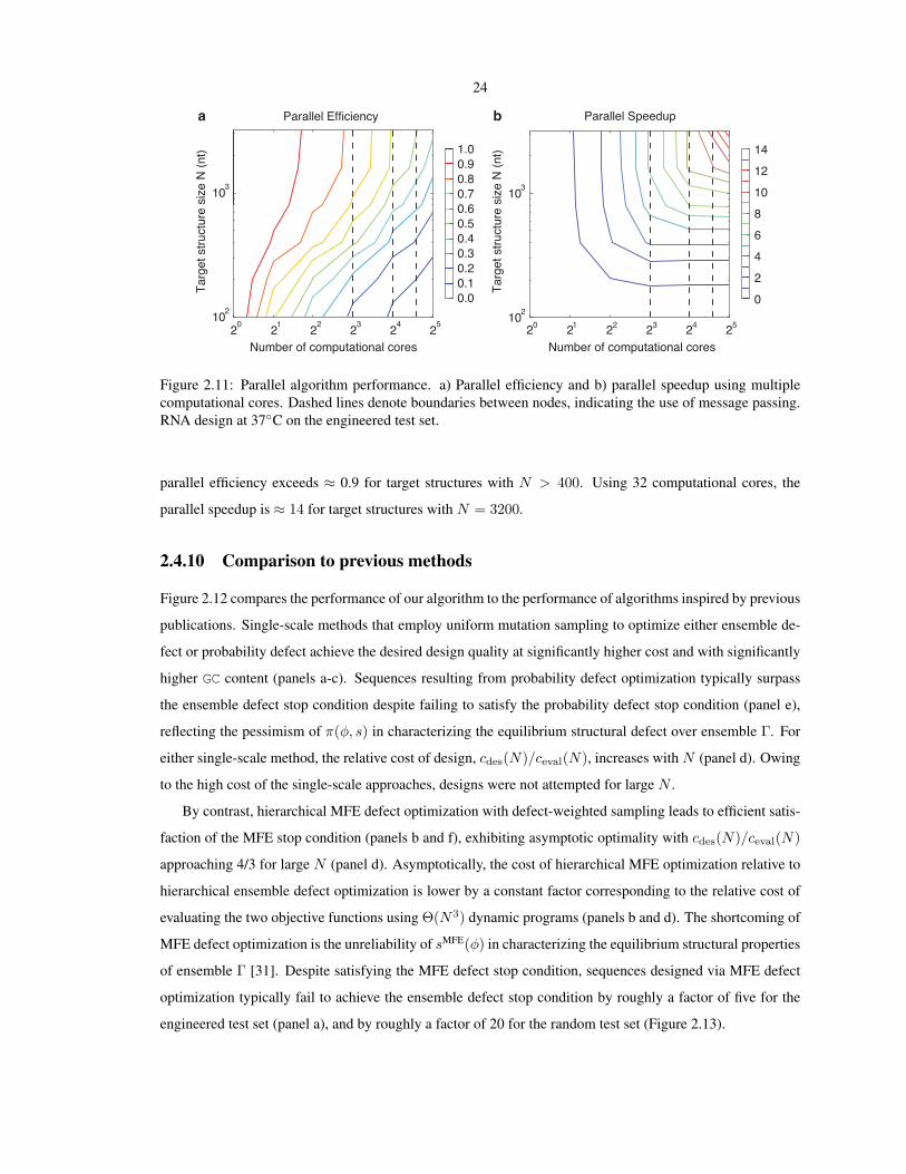
2.4.9 Parallel efficiency and speedup
The contour plots of Figure 2.11 demonstrate the parallel efficiency and speedup achieved using a parallel
implementation of the design algorithm onM computational cores (efficiency(N,M) = t(N, 1)/(t(N,M)×
M), speedup(N,M) = t(N, 1)/t(N,M), where t is wall clock time). Using two computational cores, the
3During leaf optimization, mutation candidates are not considered if they would introduce a pattern violation. Pattern violations thatarise during merging are eliminated via an adaptive walk in which mutations are accepted if they reduce the number of pattern violations.
24
0.00.10.20.3
0.50.4
0.60.70.80.91.0
Number of computational cores20 21 22 23 24 25
Targ
et st
ructu
re si
ze N
(nt)
102
103
Number of computational cores20 21 22 23 24 25
Targ
et st
ructu
re si
ze N
(nt)
102
103
0246810
1412
a bParallel Efficiency Parallel Speedup
Figure 2.11: Parallel algorithm performance. a) Parallel efficiency and b) parallel speedup using multiplecomputational cores. Dashed lines denote boundaries between nodes, indicating the use of message passing.RNA design at 37C on the engineered test set.
parallel efficiency exceeds ≈ 0.9 for target structures with N > 400. Using 32 computational cores, the
parallel speedup is ≈ 14 for target structures with N = 3200.
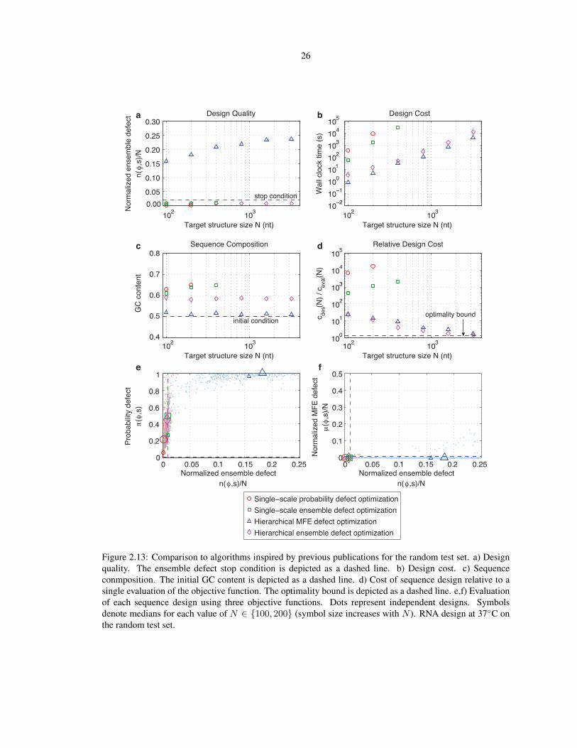
2.4.10 Comparison to previous methods
Figure 2.12 compares the performance of our algorithm to the performance of algorithms inspired by previous
publications. Single-scale methods that employ uniform mutation sampling to optimize either ensemble de-
fect or probability defect achieve the desired design quality at significantly higher cost and with significantly
higher GC content (panels a-c). Sequences resulting from probability defect optimization typically surpass
the ensemble defect stop condition despite failing to satisfy the probability defect stop condition (panel e),
reflecting the pessimism of π(φ, s) in characterizing the equilibrium structural defect over ensemble Γ. For
either single-scale method, the relative cost of design, cdes(N)/ceval(N), increases with N (panel d). Owing
to the high cost of the single-scale approaches, designs were not attempted for large N .
By contrast, hierarchical MFE defect optimization with defect-weighted sampling leads to efficient satis-
faction of the MFE stop condition (panels b and f), exhibiting asymptotic optimality with cdes(N)/ceval(N)
approaching 4/3 for large N (panel d). Asymptotically, the cost of hierarchical MFE optimization relative to
hierarchical ensemble defect optimization is lower by a constant factor corresponding to the relative cost of
evaluating the two objective functions using Θ(N3) dynamic programs (panels b and d). The shortcoming of
MFE defect optimization is the unreliability of sMFE(φ) in characterizing the equilibrium structural properties
of ensemble Γ [31]. Despite satisfying the MFE defect stop condition, sequences designed via MFE defect
optimization typically fail to achieve the ensemble defect stop condition by roughly a factor of five for the
engineered test set (panel a), and by roughly a factor of 20 for the random test set (Figure 2.13).

25
!2!1012345
0
1
2
3
4
5
0.0
0.02
0.04
0.06
0.08
0.1 No
rmali
zed
ense
mble
def
ect
n(!
,s)/N
1010101010101010
Wall
cloc
k tim
e (s
)0.4
0.5
0.6
0.7
0.8
GC co
nten
t
10
10
10
10
10
10
des
eval
c(N
) / c
(N)
0
0.005
0.010
Norm
alize
d M
FE d
efec
t"
(!,s)
/N
0
0.2
0.4
0.6
0.8
Prob
abilit
y def
ect
#(!
,s)
a b
dc
fe1
2 3 2 3
2 3 2 3
10 10
Design Quality
Target structure size N (nt)10 10
Design Cost
Target structure size N (nt)
10 10Target structure size N (nt)
Sequence Composition
10 10Target structure size N (nt)
Relative Design Cost
0 0.05 0.1Normalized ensemble defect
n(!,s)/N
0 0.05 0.1Normalized ensemble defect
n(!,s)/N
optimality boundinitial condition
stop condition
Single!scale probability defect optimizationSingle!scale ensemble defect optimizationHierarchical MFE defect optimizationHierarchical ensemble defect optimization
Figure 2.12: Comparison to algorithms inspired by previous publications for the engineered test set. a) Designquality. The stop condition for ensemble defect optimization is depicted as a dashed line. b) Design cost.c) Sequence composition. The initial GC content is depicted as a dashed line. d) Cost of sequence designrelative to a single evaluation of the objective function. The optimality bound is depicted as a dashed line. e,f)Evaluation of each sequence design using three objective functions. Stop conditions are depicted as dashedlines. Dots represent independent designs. Symbols denote medians for each value of N ∈ 100, 200(symbol size increases with N ). RNA design at 37C on the engineered test set.
26
102 1030.00 0.050.10 0.150.20 0.250.30
Design Quality
Target structure size N (nt)
Norm
alize
d en
sem
ble d
efec
tn(!,
s)/N
102 10310!210!1100101102103104105 Design Cost
Target structure size N (nt)
Wall
cloc
k tim
e (s
)
102 1030.4
0.5
0.6
0.7
0.8
Target structure size N (nt)
GC co
nten
t
Sequence Composition
102 103100
101
102
103
104
105
c des(N
) / c ev
al(N)
Target structure size N (nt)
Relative Design Cost
0 0.05 0.1 0.15 0.2 0.25
0.1
0.2
0.3
0.4
0.5
Normalized ensemble defectn(!,s)/N
Norm
alize
d M
FE d
efec
t"
(!,s)
/N
0 0.05 0.1 0.15 0.2 0.250
0.2
0.4
0.6
0.8
1
Normalized ensemble defectn(!,s)/N
Prob
abilit
y def
ect
#(!
,s)
a b
dc
fe
0
Single!scale probability defect optimizationSingle!scale ensemble defect optimizationHierarchical MFE defect optimizationHierarchical ensemble defect optimization
stop condition
initial conditionoptimality bound
Figure 2.13: Comparison to algorithms inspired by previous publications for the random test set. a) Designquality. The ensemble defect stop condition is depicted as a dashed line. b) Design cost. c) Sequenceconmposition. The initial GC content is depicted as a dashed line. d) Cost of sequence design relative to asingle evaluation of the objective function. The optimality bound is depicted as a dashed line. e,f) Evaluationof each sequence design using three objective functions. Dots represent independent designs. Symbolsdenote medians for each value of N ∈ 100, 200 (symbol size increases with N ). RNA design at 37C onthe random test set.
27
2.5 Discussion
Our algorithm combines four major ingredients to design the sequence φ of one or more strands intended to
adopt target secondary structure s at equilibrium:
• Ensemble defect optimization: The design objective function is the ensemble defect, n(φ, s), represent-
ing the average number of incorrectly paired nucleotides at equilibrium calculated over the ensemble of
unpseudoknotted secondary structures Γ. For a target structure with N nucleotides, we seek to satisfy
the stop condition: n(φ, s) ≤ fstopN .
• Hierarchical structure decomposition: We perform a binary tree decomposition of the target secondary
structure, decomposing each parent structure within a duplex stem, and introducing dummy nucleotides
to extend the truncated duplex in each child structure to mimic the parental environment.
• Leaf optimization with defect-weighted mutation sampling: Starting from a random initial sequence, se-
quence optimization is performed in the leaf nodes using defect-weighted mutation sampling in which
each candidate mutation position is selected with probability proportional to its contribution to the
ensemble defect of the leaf.
• Subsequence merging and reoptimization: As subsequences are merged moving up the tree, a parent
node initiates defect-weighted child sampling and reoptimization within its subtree only if there are
emergent defects resulting from crosstalk between child subsequences. Leaf reoptimization starts from
a new random initial sequence.
Using a Θ(N3) dynamic program to evaluate the design objective function, we derive an asymptotic opti-
mality bound on design time: for large N , the minimum cost to design a sequence with N nucleotides is 4/3
the cost of evaluating the objective function once on N nucleotides. Hence, our design algorithm has time
complexity Ω(N3).
We studied the performance of our algorithm in the context of empirical secondary structure free en-
ergy models [10, 11] that have practical utility for the analysis [36–40] and design [41–46] of functional
nucleic acid systems. In particular, we examined RNA design at 37C on target structures containing
N ∈ 100, 200, 400, 800, 1600, 3200 nucleotides and duplex stems ranging from 1 to 30 base pairs. Empir-
ically, we observe several striking properties:
• Emergent defects are sufficiently infrequent that they can typically be eliminated by leaf reoptimization
starting from new random initial sequences.
• It is routine to design sequences with ensemble defect n(φ, s) < N/100 over a wide range of GC
contents.

28
• Our algorithm exhibits asymptotic optimality for large N , with full sequence design costing roughly
4/3 the cost of a single evaluation of the objective function. Hence, the algorithm is efficient in the
sense that the exponent in the Ω(N3) time complexity bound is sharp.
We modified our algorithm to compare performance to algorithms inspired by previous work [20, 27–29,
31, 32]. In line with conceptual expectations, we observe empirically that our algorithm achieves lower design
cost relative to single-scale probability or ensemble defect optimization with uniform mutation sampling, and
higher design quality relative to hierarchical MFE defect optimization with defect-weighted sampling.
To enhance the utility of our algorithm for molecular engineers, our algorithm addresses several practi-
cal considerations, including: sequence constraints, pattern prevention, multi-stranded target structures, and
parallel execution.

29
Chapter 3
Sequence design for multi-state nucleicacid systems
Motivated by the design of multi-state nucleic acid systems [41, 44–47], we wish to extend the quality and
efficiency of the single-complex algorithm to the design of multiple strands that interact conditionally to form
multiple different target structures. Most of these dynamic systems involve pathways of interactions between
complexes. For instance, a disassembly reaction involving one complex might release a strand that engages
in a self-assembly reaction with another complex. For these types of interactions to occur, the identities of
certain bases across the multiple ordered complexes may be linked.
Our early approaches to using ensemble defect optimization for the design of multi-state systems em-
ployed single-scale algorithms. These algorithms successfully designed systems that exhibited the desired
behavior [41, 44, 45], but were costly, as one would expect from our single-scale computational studies pre-
sented in Chapter 2. Here we extend the scope of our single-complex design algorithm to include the design
of multiple ordered complexes with related sequences.
3.1 Objective function
The design of multiple ordered complexes can be formulated as a multiobjective optimization problem, min-
imizing the ensemble defect of each sequence in Φ = φ1, ..., φR relative to a set of target structures
Ψ = s1, ..., sR simultaneously,
n(φt, st) < fstopNt ∀st ∈ Ψ.
Thus, we wish to achieve the same single-objective stop condition on each ordered complex in Ψ. In order to
maintain the efficiency and quality, our approach preserves the same algorithmic ingredients from the single-
objective problem: each structure in Ψ undergoes hierarchical structure decomposition, leaf optimization with
weighted mutation sampling, and subsequence merging with weighted leaf sampling and reoptimization.

30
3.2 Sequence linkages
In addition to providing a set of ordered complexes Ψ, the algorithm also requires a set of linkages Ξ =
η1, ..., ηz where each linkage η is a quintuple 〈sa, i, sb, j, ρ〉 representing the base-pairing relationship
ρ ∈ complementary, identical between the base at position i in complex sa and the base at position j
in complex sb. Thus, in Φ, base i in sequence φa must be either complementary or identical to base j in
sequence φb. Furthermore, linkages can exist within the same structure (i.e., sa = sb) and each base can
participate in multiple linkages.
3.3 Optimality bound and time complexity
Since the multiobjective algorithm is attempting to design multiple decomposition trees simultaneously, the
asymptotic optimality bound is the sum over the bounds of designing those trees independently and is given
by
cdes(Ψ) ≥ 43
∑s∈Ψ
ceval(s).
3.4 Multiobjective ensemble defect optimization algorithm
3.4.1 Synchronizing linkages
The existence of a set of linkages Ξ implies that a mutation at one base could potentially affect multiple other
bases elsewhere in the system. To keep bases in sync, the algorithm employs a global sequence table, GST,
with each entry corresponding to a base identity. The quintuples in Ξ are used to assign a global index in this
table to each base position in each structure st ∈ Ψ. Thus, in the quintuple 〈sa, i, sb, j, ρ〉, position i in sa
and position j in sb will be assigned the same global index as will all other linked related bases. In addition
to each base being assigned an index in the GST, each base will also be assigned a relationship ρ to that entry
in the GST.
Each mutation requires an update to the global sequence table. It also follows that prior to objective
function evaluation, all bases will be synchronized with the the global sequence table.
3.4.2 Multi-state hierarchical decomposition
Each structure in Ψ is decomposed with the same single-complex technique outlined in Section 2.2.1. The
decomposition process also ensures that each base in the decomposition tree also has the appropriate GST
index.
We will refer to the set of all nodes in all decomposition trees as ΨD and the leaves as ΨL ⊆ ΨD.
Individual nodes, skt , are uniquely identified by their tree t and node index k.

31
3.4.3 Multi-leaf optimization with weighted mutation sampling
The algorithm makes mutations to nodes in ΨL with the goal of satisfying the stop condition
n(φkt , skt ) ≤ fstop|skt | ∀skt ∈ ΨL.
To determine which leaves are not satisfied and thus eligible for mutation, we define an ensemble defect
threshold function,
nthreshold(φkt , skt ) =
n(φkt , skt ) : n(φkt , s
kt ) > fstop|skt |
0 : n(φkt , skt ) ≤ fstop|skt |
,
that is used to weigh which leaf should be optimized next. The probability of a selecting a leaf sk∗
t∗ for
mutation is nthreshold(φk∗
t∗ , sk∗
t∗ )/∑sk
t∈ΨL nthreshold(φkt , skt ). Once a leaf is selected, mutations are weighted
according to the same defect sampling scheme of the single-complex algorithm, described in Section 2.2.2.
After a mutation is made, the other leaves must be synchronized with the GST. To determine if the
mutation brought the multiple objectives closer to the stop condition, we calculate n(φkt , skt ) for each leaf
and sum the thresholding functions. The mutation is retained if
∑sk
t∈ΨL
nthreshold(φkt , skt ) <
∑sk
t∈ΨL
nthreshold(φkt , skt ).
Thus, when ∑sk
t∈ΨL
nthreshold(φkt , skt ) = 0,
the stop condition has been reached.
As in single-complex design, we keep a list of previously rejected mutations, γkt , for each leaf1. Thus, a
mutation that propagates to several other leaves must be retained in each leaf’s γkt list. If leaf skt accepts a
mutation, even if that mutation originated elsewhere, it must clear its γkt list. Likewise, any failed mutation
must be stored locally in each affected leaf’s γkt .
Optimization of leaves terminates successfully if the stop condition is satisfied or unsuccessfully if
Munfavorable|skt | consecutive unfavorable candidate mutations are either in γkt or are evaluated and added
to γkt for all leaves skt ∈ ΨL.
This leaf optimization procedure is reinitialized and reoptimized up to Mleafopt times. With each at-
tempt, leaves that did not satisfy the stop condition are reinitialized. Note that reinitialization may propagate
mutations to leaves that were previously satisfied.
1In the single-complex algorithm, we maintained only one γunfavorable since only one leaf was optimized at a time. However, inthe multiobjective case we must maintain separate lists γk
t , hence the need for indexing notation.

32
3.4.4 Subsequence merging and reoptimization
Once the leaves have been optimized, the algorithm can begin checking merged substructures and moving up
the tree. Just as leaf optimization occurred on set ΨL ⊆ ΨD, we generate a new set of nodes for evaluation
ΨK ⊆ ΨD where K is an integer representing a level in the tree starting with K = max(depth(k)). This set
is defined as
ΨK = skt ∈ ΨD : depth(k) = K ∪ skt ∈ ΨL : depth(k) < K.
This set represents all nodes at the same level K and any leaves that have a shallower tree depth than K (i.e.,
depth(k) < K). When K = 1, the algorithm has reached the global objective function. Therefore, Ψ1 = Ψ
and Ψmax(depth(k)) = ΨL. Figure 3.1 illustrates leaf, parent, and root node sets.
Reoptimization decisions are made in the same manner as single-complex design. All nodes in ΨK where
K < max(depth(k)) that are unsatisfied will select a reopt child in ΨK+1 using defect weighted sampling.
This will continue down the tree, bringing inherited information, until ΨL is encountered. The reopt leaves
of ΨL are reinitialized (perhaps affecting other previously satisfied leaves) and redesigned from new random
initial sequences.
Upon subsequent mergings, the algorithm determines which nodes improved and updates their sequences
in the GST without overwriting other nodes that were previously satisfied. This requires looking at sets of
linked nodes to see if the overall behavior of an entire linked-node-set improved.
3.4.5 Language
Since it would be cumbersome for a molecular engineer to manually specify each linkage for even a modest
sized system, we have developed a scripting language that aids in describing linked, multi-state systems.
A user begins by defining target structures and sequence blocks. Sequence blocks are regions of contiguous
bases that might be linked to other regions elsewhere in the system. With sequence blocks, instead of defining
linkages on a base-by-base basis, a user can define linkages on a region-by-region basis. After structures and
sequence blocks are defined, the user must indicate how the blocks are arranged on the target structure from
the 5′ end to the 3′ end. Finally, the user must indicate which structures are to be included the objective
function and the desired fstop of each objective.
Defining structures
Structures are defined using the following statement:
structure struc name = s
where s is a secondary structure in Ψ that can be specified in either dot-parens-plus notation or HU+ notation
(see Appendix D).

33
a) Leaf optimization
b) Parent node evaluation
c) Root node evaluation
Figure 3.1: Example of multiobjective decomposition trees. a) Leaf optimization is performed on the set ofleaves ΨL in the tree, shaded in green. b) After leaf optimization, the algorithm proceeds up the tree to Ψ2
which includes the leaves shaded in red and pink. The leaves shaded in pink were already satisfied so theyneed not be considered again. c) The set Ψ1 = Ψ contains the roots of all trees, shaded in red and pink. Thered nodes must be evaluated.

34
Defining sequences
A sequence block is defined using the following statement:
sequence seq name = constraints
where constraints is an array of strings, each of the form X1C1, delimited by spaces, where Xi is the number
of bases of type Ci.
The complement sequence block seq name* is generated automatically and represents the reverse comple-
ment of seq name; it must also adhere to the complement constraints (i.e., the complement of 5W is 5S).
Linking structures and sequence blocks
The linkages between structures are defined by specifying the sequence blocks of a structure. Two structures
with the same sequence block will have an identical sequence at the block’s respective position.
struc name : sequence array
where sequence array is a comma delimited array of sequence block identifiers. For example,
I : c d c*
is interpreted to mean that the structure I is made up of the sequence blocks c, d, and c* when read from 5′
to 3′. The sum of the lengths of the sequence blocks must be identical to the length of the structure.
Defining stop conditions
The stop condition of each objective function is set by using the following line:
struc name < fstop
Allowing for varying fstop by objectives allows the molecular engineer to enforce varying degrees of
quality for different structures in the system.
Example script
A complete example script for a programmable in situ amplification system [46] is shown in Algorithm 3.2.
3.4.6 Implementation and comparison to single-complex design
Pseudocode for the multiobjective algorithm is provided in Algorithm 3.1. Unlike the single-complex algo-
rithm, the implementation of this multiobjective algorithm is not recursive. Even though there are multiple
structural decomposition trees, the nodes of these trees are partitioned into sets that are designed together.
While the algorithm designs leaves and evaluates parent nodes in a different order compared to the single-
complex algorithm, it is performing tasks with all of the same algorithmic ingredients. We thus expect a
correct implementation of the multiobjective algorithm to perform similarly for single-complex input.
The multiobjective algorithm is implemented with object oriented programming in C++.

35
structure H1 = U10 H16 (U10)structure H2 = H16 (U10) U10structure I1 = U26structure I2 = U26structure I1H1 = H26 (+) U26structure I2H2 = U26 H26 (+)structure R1 = U10structure R2 = U10sequence a = 10Nsequence b = 16Nsequence c = 10NH1 : a b c* b*H2 : b* a* b cI1 : b* a*I2 : c* b*I1H1 : b* a* a b c* b*I2H2 : b* a* b c c* b*R1 : aR2 : cH1 < 1.0H2 < 1.0I1 < 1.0I2 < 1.0I1H1 < 1.0I2H2 < 1.0
Figure 3.2: Code for programmable in situ amplification for multiplexed bioimaging [46]. This system isdesigned with RNA energy parameters at 45 C.
3.5 Computational studies
For comparison with the single-complex algorithm, we ran our algorithm on the engineered and random sets
used in Chapter 2. As shown in Figures 3.3 and 3.4 our multiobjective algorithm performs similarly to the
single-complex algorithm although with greater cost.
To demonstrate the multiobjective algorithm’s efficacy in designing nucleic acid systems invented by
molecular engineers, we created a test suite of 8 systems with code for each given in Appendix B. We evalu-
ated the design of these systems for quality and cost compared to an single-scale unweighted ensemble defect
optimization approach. The results, shown in Figure 3.5, demonstrate that our hierarchical multiobjective
algorithm achieves similar quality as the single-scale approach. For larger systems the hierarchical algorithm
has a significantly lower cost since it can create larger decomposition trees. For the larger systems we achieve
more than an order of magnitude cost improvement without loss in quality.
In Figure 3.6 we present results of an imperfect design for a system that allows for programmable in situ
amplification for multiplexed bioimaging [46]. As demonstrated, the majority of the sequences have achieved
low ensemble defect for their target structures. There are linked bases, however, that exist in multiple contexts,
and do not form desired base-pairs with high probability.

36
DESIGNOBJECTIVES(ΨD,GST)
for s ∈ ΨL
s.reseed← TRUE
for s ∈ ΨD −ΨL
s.mreopt ←Mreopt
satisfied← FALSEwhile not satisfied
DESIGNLEAVES(ΨL,GST)satisfied←
MERGELOOP(ΨD,GST)return ΨD,GST
DESIGNLEAVES(ΨL,GST)
for s ∈ ΨL
s.munfavorable ←Munfavorable · s.NPQ.CLEAR()ΨL.RESETBEST()satisfied← FALSEmredesign ← 0while not satisfied and
mredesign < Mredesign + 1res← GETRESEEDEDSTRUCTS()INITRANDOM(res)
ΨL,mut← OPTIMIZELEAVES()satisfied← NODESSATISFIED()mredesign ← mredesign + 1if mredesign < Mredesign + 1
u← GETUNSATISFIED(mut)for s ∈ u
s.reseed← TRUE
ΨL.UPDATEBEST(ΨL)ΨL.REVERTTOBEST(GST)
MERGELOOP(ΨD,GST)
satisfied← TRUEk ← LEAFDEPTH − 1while satisfied and k ≥ 0
UPDATELEVEL(Ψk)while PQ.SIZE > 0
UPDATEDEFECT(PQ.TOP)PQ.POP()
Ψk.UPDATEBEST()Ψk.REVERTTOBEST(GST)for s ∈ Ψk
if s.n > f · s.N andnot s ∈ ΨL
satisfied← FALSE
REDESIGN(s,ΨD)k ← k − 1
return satisfied
REDESIGN(s,ΨD)
s.mreopt ← s.mreopt − 1s← swhile not s ∈ ΨL
nleft, nright ← s.MAPCHILDREN()r ← RANDOM(0, nleft + nright)if r < nleft
s← s.GETLEFTCHILD()else
s← s.GETRIGHTCHILD()s.mreopt ←Mreopt
ΨD.RESETLEVEL(s.DEPTH)s.mreopt ←Mredesign
s.reseed← TRUE
OPTIMIZELEAVES(ΨL,GST)
mut← ∅UPDATELEVEL(ΨL)while PQ.SIZE > 0
ψ ← PQ.TOPif not PQ.TOP in mut
mut.INSERT(PQ.TOP)UPDATEDEFECT(s,GST)
ΨL ← ΨL
ΨL.RESETBEST()leaves satisfied← FALSEwhile not leaves satisfied
s← PICKGUIDEDSTRUCTURE(ΨL,mut)ξ ← WEIGHTEDMUTATION(s)if ξ ∈ s.γunfavorable
s.munfavorable ← s.munfavorable − 1else if CAUSESCONFLICT(ξ)
s.munfavorable ← s.munfavorable − 1s.γunfavorable ← s.γunfavorable ∪ ξ
elseΨL ← APPLYMUTATION(ξ, ΨL)
UPDATELEVEL(ΨL)modified← ∅while PQ.SIZE > 0
modified.APPEND(PQ.TOP)if not PQ.TOP in mut
mut.INSERT(PQ.TOP)UPDATEDEFECT(PQ.TOP,GST)PQ.POP()
success← ΨL.UPDATEBEST(ΨL)if success
for s ∈ modifieds.munfavorable ← 4 · s.Ns.γunfavorable ← ∅
elsefor s ∈ modified
s.munfavorable ← s.munfavorable − 1s.γunfavorable ← s.γunfavorable ∪ ξ
ΨL.REVERTTOBEST(GST)leaves satisfied← LEAVESSATISFIED(mut)
return ΨL,mut
Algorithm 3.1: Pseudocode for multiobjective, hierarchical ensemble optimization with weighted mutationsampling.
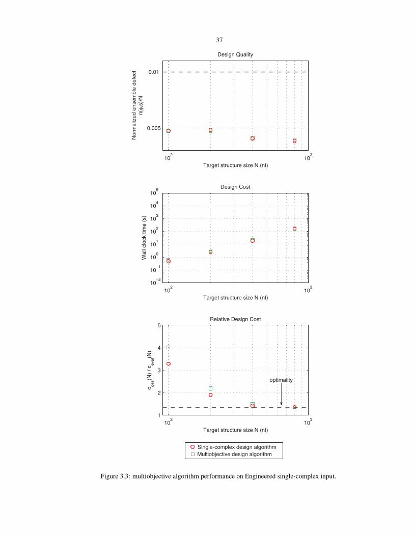
37
102 103
0.005
0.01
Design Quality
Target structure size N (nt)
Nor
mal
ized
ens
embl
e de
fect
n(φ,
s)/N
102 10310−210−1100
101
102
103
104
105 Design Cost
Target structure size N (nt)
Wal
l clo
ck ti
me
(s)
102 1031
2
3
4
5
c des(N
) / c
eval(N
)
Target structure size N (nt)
Relative Design Cost
Single-complex design algorithm
optimality
Multiobjective design algorithm
Figure 3.3: multiobjective algorithm performance on Engineered single-complex input.

38
102 103
0.005
0.01
Design Quality
Target structure size N (nt)
Nor
mal
ized
ens
embl
e de
fect
n(φ,
s)/N
102 10310−210−1100
101
102
103
104
105 Design Cost
Target structure size N (nt)
Wal
l clo
ck ti
me
(s)
102 1031
10
20
30
40
50
c des(N
) / c
eval(N
)
Target structure size N (nt)
Relative Design Cost
optimality
Single-complex design algorithmMultiobjective design algorithm
Figure 3.4: multiobjective algorithm performance on Random single-complex input.
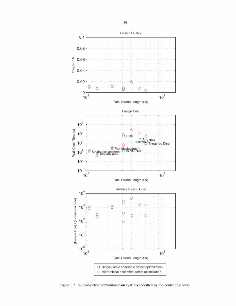
39
102 1030
0.02
0.04
0.06
0.08
0.1Design Quality
Σn(φ,
s) / Σ
N
Total Strand Length (ΣN)
102 10310−1
100
101
102
103
104
Total Strand Length (ΣN)
Design Cost
Wal
l Clo
ck T
ime
(s)
Seesaw gate Pair displacement
Triggered Dicer And gate
Single displacement
HCR
in situ HCR
Rickettsia
102 103100
101
102
103
104
Total Strand Length (ΣN)
(Des
ign
time)
/ (E
valu
atio
n tim
e)
Relative Design Cost
Single−scale ensemble defect optimizationHierarchical ensemble defect optimization
Figure 3.5: multiobjective performance on systems specified by molecular engineers.

40
Equilibrium probability
H1 H2
I1
I2
I2H2
I1H1
Figure 3.6: multiobjective design results for an imperfect programmable in situ amplification system. Thebases with the largest defect are a base-pair at the end of helix in the structure I2H2. The purple and brownarrows demonstrate the other locations in the system where these bases are linked, which exhibit low defectfor these bases.

41
3.6 Discussion
Our algorithm designs a set of sequences Φ for the set of linked structures Ψ by utilizing the four major in-
gredients from single-complex design: ensemble defect optimization, hierarchical structure decomposition,
leaf optimization with weighted sampling, and subsequence merging with weighted leaf sampling and reop-
timization. To ensure that linkages are preserved, leaf optimization, merging, and reoptimization all occur
at each depth in the tree simultaneously. The bound on running time is 4/3 the summed cost of a single
evaluation of each objective in Ψ. To aid molecular engineers in specifying systems, we have also developed
a scripting language for expressing target structures and the linkages between them.
We studied the performance of our algorithm on invented nucleic acid systems. Our results demonstrate
that this algorithm achieves high-quality design but with a cost significantly higher than the optimum. Cost
is improved, relative to single-scale methods, as the input systems grow larger. We also ran this algorithm on
single-complex input and achieved similar results to our previous single-complex studies.
Linkages provide an inherent challenge for designing multi-state systems. Although linked bases may
have the same identity (or be complementary) they must be designed to perform well in a variety of contexts.
For example in systems similar to the programmable in situ amplification system [46], some linked bases are
unpaired in some structures and paired in others. Base identities that stabilize the unpaired regions may not
be ideal for stabilizing helix regions.
Furthermore, the development of a multiobjective algorithm is strongly motivated by the inventions of
molecular engineers. Although the invented systems studied in this chapter have multiple objectives, the
individual objectives of some of the systems are small and thus do not benefit from the efficiency provided
by hierarchical decomposition. Furthermore, the heterogeneity of the invented design objectives provide a
challenge in observing how the algorithm performs relative to the optimum. Further computational studies
are needed in order to characterize the performance of this algorithm. By creating test sets that allow us to
vary objective size, the size of Ψ, the number of linkages, and the nature of those linkages, we may be able
to improve the performance of algorithm and fully describe why the cost of designing our set of invented
structures is relatively high.

42
Chapter 4
The NUPACK web server: analysis anddesign of nucleic acid systems
The work in this chapter is based on the following submitted manuscript: J. N. Zadeh, C. Steenberg, J. S.
Bois, B. R. Wolfe, M. B. Pierce, A. Khan, R. Dirks, and N. A. Pierce. NUPACK: Analysis and design of
nucleic acid systems.
4.1 Introduction
In the two previous chapters we described methods for achieving high-quality sequence design for systems
of interacting nucleic acid strands with improved computational cost. In order to increase the ease of use
and accessibility of these and other related algorithms, we have developed NUPACK, an online server for the
analysis and design of nucleic acid systems, available at http://nupack.org.1
A web application is an attractive platform as a front-end for computational tools. Not only does this
lower the technological barrier for users since the only requirement is that their system have a compatible
web browser, it allows us to develop for a single platform and continuously release new features without
requiring global redistribution. Furthermore, a centralized web application like NUPACK allows the research
community to share a single high-performance compute cluster, a resource which might otherwise be un-
available, over commodity Internet.
The are currently two other independent software packages for analyzing the structure of nucleic acids:
UNAFold (previously mfold) [48, 49] and RNAFold [20, 50]. Both packages and accompanying web
servers can perform partition function and minimum free energy calculations on sequences for single strands
or dimers. 2 An additional resource, the RNASoft web server can also perform MFE calculations on
dimers [52].3 The RNAFold, RNAsoft [27], and INFO-RNA [28, 53] design servers perform MFE defect
1Note that at the time of this writing, not all of the features described here are publicly available. Those features are available as aprivate beta feature for a select group of users.
2The DINAMelt package [51] extends UNAFold’s capabilities of predicting dimer structures.3 RNASoft also offers source code download for MultiRNAFold package for MFE prediction of an arbitrary number of interacting
nucleic acids [24].

43
optimization using the RNAFold engine for computing their objective function. The RNAFold design server
also offers a single-scale probability optimization design algorithm.
NUPACK is focused on the analysis and design of systems involving an arbitrary number of interacting
strands. Notable features include:
• calculation of the partition function and minimum free energy (MFE) secondary structure for unpseu-
doknotted complexes of arbitrary numbers of interacting RNA or DNA strands4 including rigorous
treatment of distinguishability issues that arise in the multi-stranded setting [8].
• calculation of the equilibrium concentrations for arbitrary species of complexes in a dilute solution
(e.g., for a test tube of interacting RNA or DNA strand species) [8].
• use of partition function and concentration information to calculate equilibrium base-pairing observ-
ables for dilute solutions of interacting strand species [8].
• partition function analysis of non-interacting RNA strands including the possibility of a class of pseu-
doknots [22, 33].
• sequence design for one or more strands intended to adopt an unpseudoknotted target secondary struc-
ture at equilibrium (see Chapter 2).
• sequence design for multiple, linked, unpseudoknotted target secondary structures at equilibrium (see
Chapter 3).
The NUPACK web server also offers utilities for the customization of figures for talks and papers, providing
• publication-quality vector graphics that can be downloaded and edited in standard vector graphics
programs.
• automatic layout and rendering of secondary structures depicted with or without ideal helical geometry.
• dynamic graphical editing of secondary structure layout within the web interface.
4.2 Application organization
NUPACK’s web application is organized into three interconnected modules: Analysis, Design, and Utilities.
Each of these modules can export results to the other two modules for further computation. The functionality
and relationships between the modules are summarized Figure 4.1.
The modules can be accessed via the orange navigation bar at the top of each page, as shown in Figure 4.2.
The green navigational bar provides a submenu of items relevant to the current module. Located in this
4The web server currently limits the maximum complex size to ten strands and displays a single MFE structure. Larger complexesand degenerate MFE structures can be analyzed by downloading and compiling the NUPACK source code.
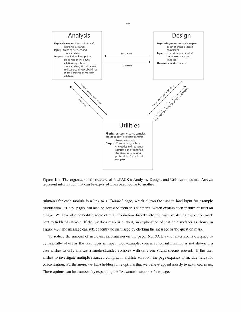
44
structure
sequence
UtilitiesPhysical system: ordered complexInput: strand sequencesOutput: Customized graphics, energetics and sequence
structure, base-pairing probabilities for ordered complex
DesignPhysical system: ordered complex or set of linked ordered complexesInput: target structure or set of target structures and linkagesOutput: strand sequences
AnalysisPhysical system: dilute solution of interacting strandsInput: strand sequences and concentrationsOutput: equilibrium base-pairing properties of the dilute solution; equilibrium concentration, MFE structure, and base-pairing probabilities of each ordered complex in solution.
target s
tructu
re, sequence
MFE structure, sequence
sequence
Figure 4.1: The organizational structure of NUPACK’s Analysis, Design, and Utilities modules. Arrowsrepresent information that can be exported from one module to another.
submenu for each module is a link to a “Demos” page, which allows the user to load input for example
calculations. “Help” pages can also be accessed from this submenu, which explain each feature or field on
a page. We have also embedded some of this information directly into the page by placing a question mark
next to fields of interest. If the question mark is clicked, an explanation of that field surfaces as shown in
Figure 4.3. The message can subsequently be dismissed by clicking the message or the question mark.
To reduce the amount of irrelevant information on the page, NUPACK’s user interface is designed to
dynamically adjust as the user types in input. For example, concentration information is not shown if a
user wishes to only analyze a single-stranded complex with only one strand species present. If the user
wishes to investigate multiple stranded complex in a dilute solution, the page expands to include fields for
concentration. Furthermore, we have hidden some options that we believe appeal mostly to advanced users.
These options can be accessed by expanding the “Advanced” section of the page.
45
Figure 4.2: The NUPACK web application navigational bar with links to the Analysis, Design, and Utilitiesmodules highlighted in orange. Submenu items that are related to the current module, such as “Demos” and“Help”, are highlighted in green.
Figure 4.3: When a user clicks the orange-highlighted question mark, a help popup appears, providing infor-mation relevant to the feature or field.
4.3 Publication-quality graphics
The standard convention for drawing two-dimensional nucleic acid secondary structures is to depict helix
regions as rectangles and loop regions as circles. Base pairs are also connected by line segments. Using
this convention it is not possible to draw all secondary structures without distorting distances between bases
or allowing structural elements to overlap.5 The first published drawing algorithms attempted to prevent
overlapping substructures by allowing the user to interactively “untangle” the illustration [48, 50, 54, 55].
Subsequent drawing algorithms attempt to automatically deform structural elements to prevent overlaps [56,
57]. As a consequence, users do not have precise control over the layout and aesthetics of the drawing.
Recent nucleic acid drawing software enables the user to interactively modify or untangle canonical struc-
tures [58, 59]. NUPACK also utilizes this approach of drawing structures without deformation and allowing
the user to edit the structure in a manner they find pleasing. To this end, we have developed an in-browser
nucleic acid drawing editor that runs natively in the browser. With this integrated editor, shown in Figure 4.4,
the user can shrink or grow unpaired loop regions, stretch helices, or change the angle of stems relative to
adjacent loops.
NUPACK offers several options for drawing two-dimensional secondary structures. Bases can be repre-
sented by ticks or circles that can be shaded according to their identity (i.e., A, G, C, or T/U) or the probability
they are paired at equilibirum. Bases can also be annotated with their numerical position in the structure
and with their base identity. Figure 4.5 demonstrates some examples of different shading options. Two-
dimensional structures can also be rendered with their backbones and bases displaying ideal helical geome-
try, shown in Figure 4.6. These can also be edited within the NUPACK interface. NUPACK also provides
5An example of a structure impossible to draw without overlaps or distance distortion is shown in Figure 4.4 a. In this case, four-branch multiloops will inevitably overlap each other.

46
a)
e)
b)
c)
d)
Figure 4.4: NUPACK offers an in-browser secondary structure editor that does not require the installation ofthird-party software. One method of untangling the structure depicted in a) is to activate the editor, shown inb). The angle of a branch in a multiloop can be changed, shown in c). A helix can also be stretched, shown ind). Once the “Update” button is selected, the NUPACK server will re-render the images with new orientation,depicted in e).
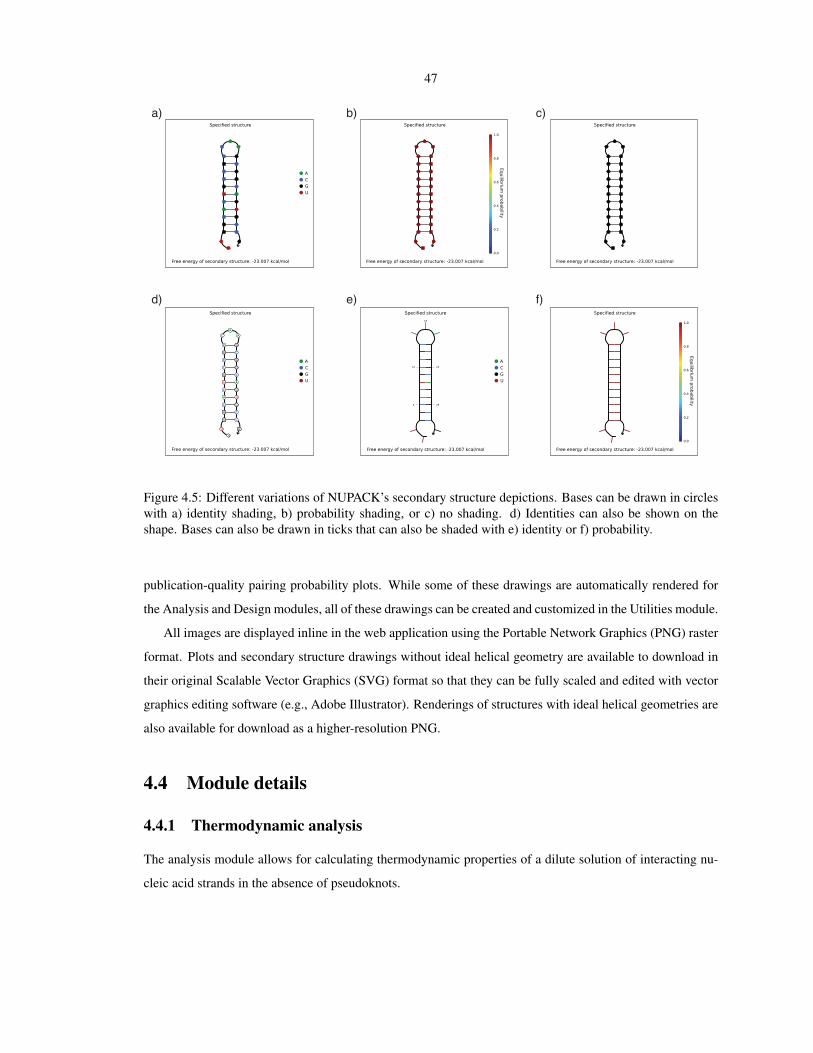
47
a) b) c)
d) e) f)
Figure 4.5: Different variations of NUPACK’s secondary structure depictions. Bases can be drawn in circleswith a) identity shading, b) probability shading, or c) no shading. d) Identities can also be shown on theshape. Bases can also be drawn in ticks that can also be shaded with e) identity or f) probability.
publication-quality pairing probability plots. While some of these drawings are automatically rendered for
the Analysis and Design modules, all of these drawings can be created and customized in the Utilities module.
All images are displayed inline in the web application using the Portable Network Graphics (PNG) raster
format. Plots and secondary structure drawings without ideal helical geometry are available to download in
their original Scalable Vector Graphics (SVG) format so that they can be fully scaled and edited with vector
graphics editing software (e.g., Adobe Illustrator). Renderings of structures with ideal helical geometries are
also available for download as a higher-resolution PNG.
4.4 Module details
4.4.1 Thermodynamic analysis
The analysis module allows for calculating thermodynamic properties of a dilute solution of interacting nu-
cleic acid strands in the absence of pseudoknots.

48
Figure 4.6: Depiction of secondary structures with ideal helical geometry for stacked base pairs, as for thiscomplex of three DNA strands with B-form helices (left) or three RNA strands with A-form helices (bottom).
Input
The Analysis input page allows the user to specify the components and conditions of the solution of interest:
• RNA or DNA.
• Temperature (or range of temperatures for melts).
• Number of strand species.
• Maximum complex size (all ordered complexes with up to this number of strands will be included in
the analysis).
• Strand sequences.
• Strand concentrations (for calculations with maximum complex size greater than one).
Under an expandable Advanced Options panel, users may select among available energy models, specify
salt concentrations, allow a class of pseudoknots (non-interacting RNA strands only), and specify additional
ordered complexes to include in the calculation (larger than the specified maximum complex size). The
estimated computation time is displayed as the user provides input. If this estimate is on the order of hours,
an email address is required to notify the user of job completion; jobs estimated to exceed a threshold are not
accepted.
Computation
The partition function, equilibrium base-pairing probabilities, and MFE structure are calculated for each
ordered complex using dynamic programs [8, 22, 33]. For calculations in which the maximum complex size
is greater than one, the calculated partition functions and user-provided strand concentrations are used to
calculate the equilibrium concentration of each ordered complex by solving a convex optimization problem
[8]. If the user wishes to change the strand concentrations after examining the results, it is not necessary
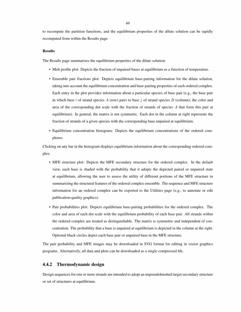
49
to recompute the partition functions, and the equilibrium properties of the dilute solution can be rapidly
recomputed from within the Results page.
Results
The Results page summarizes the equilibrium properties of the dilute solution:
• Melt profile plot: Depicts the fraction of unpaired bases at equilibrium as a function of temperature.
• Ensemble pair fractions plot: Depicts equilibrium base-pairing information for the dilute solution,
taking into account the equilibrium concentration and base-pairing properties of each ordered complex.
Each entry in the plot provides information about a particular species of base pair (e.g., the base pair
in which base i of strand species A (row) pairs to base j of strand species B (column); the color and
area of the corresponding dot scale with the fraction of strands of species A that form this pair at
equilibrium). In general, the matrix is not symmetric. Each dot in the column at right represents the
fraction of strands of a given species with the corresponding base unpaired at equilibrium.
• Equilibrium concentration histogram: Depicts the equilibrium concentrations of the ordered com-
plexes.
Clicking on any bar in the histogram displays equilibrium information about the corresponding ordered com-
plex:
• MFE structure plot: Depicts the MFE secondary structure for the ordered complex. In the default
view, each base is shaded with the probability that it adopts the depicted paired or unpaired state
at equilibrium, allowing the user to assess the utility of different portions of the MFE structure in
summarizing the structural features of the ordered complex ensemble. The sequence and MFE structure
information for an ordered complex can be exported to the Utilities page (e.g., to annotate or edit
publication-quality graphics).
• Pair probabilities plot: Depicts equilibrium base-pairing probabilities for the ordered complex. The
color and area of each dot scale with the equilibrium probability of each base pair. All strands within
the ordered complex are treated as distinguishable. The matrix is symmetric and independent of con-
centration. The probability that a base is unpaired at equilibrium is depicted in the column at the right.
Optional black circles depict each base pair or unpaired base in the MFE structure.
The pair probability and MFE images may be downloaded in SVG format for editing in vector graphics
programs. Alternatively, all data and plots can be downloaded as a single compressed file.
4.4.2 Thermodynamic design
Design sequences for one or more strands are intended to adopt an unpseudoknotted target secondary structure
or set of structures at equilibrium.

50
Input
The design input page allows the user to specify design requirements:
• RNA or DNA.
• Temperature.
• Number of independent sequence designs.
• Target secondary structure in dot-parens-plus notation (each unpaired base is represented by a dot, each
base pair by matching parentheses, and each nick between strands by a plus). A user can also specify
multiobjective designs by using the language described in Appendix D.
Target secondary structures for single-complex design that are multi-stranded must be connected. Valid target
structures are depicted during data entry to provide visual feedback to the user. Under an expandable Ad-
vanced Options panel, users may select among available energy models, specify salt concentrations, specify
sequence constraints, and define pattern prevention requirements.
Computation
The design algorithm performs efficient ensemble defect optimization to reduce the ensemble defect [31].
For a target secondary structure withN nucleotides, the algorithm seeks to achieve an ensemble defect below
N/100 (see Chapter 2). For a set of target secondary structures, the algorithm seeks to achieve the same
condition for each objective.
Results
The Results page summarizes the properties of the designed sequences:
• Designability summary: Depicts each base in the target secondary structure shaded by the probability
that it adopts the depicted paired or unpaired state at equilibrium, averaged across the independent
sequence designs. This plot can expose conceptual design flaws in the target structure: if a particular
base pair has a low probability of forming over several independent sequence designs, adjustments to
the target structure may be warranted.
• Sequence designs table: Displays the ensemble defect, normalized ensemble defect, GC content of
each design, and sequences for each design.
Any set of designed sequences can be exported to the Analysis page (e.g., to check for the formation of
unintended ordered complexes in the context of a dilute solution) or to the Utilities page (e.g., to customize
publication-quality graphics). Alternatively, clicking on a sequence design displays equilibrium information
about the ordered complex to which the target secondary structure belongs:

51
• Target structure plot: Depicts the target secondary structure with each base shaded by the probability
that it adopts the depicted state at equilibrium.
• Pair probabilities plot: Depicts the equilibrium base-pairing probabilities for the ordered complex.
Optional black circles depict each base pair or unpaired base in the target secondary structure.
4.4.3 Utilities
The Utilities page accepts as input either sequence information, structure information, or both, performing
diverse functions based on the information provided, including
• Evaluation and display of equilibrium information for an arbitrary secondary structure in the context
of the ordered complex to which it belongs (analogous to the treatment of the MFE structure in the
Analysis page, and the target structure in the Design page).
• Redimensioning duplex and loop lengths in a secondary structure while retaining the original sequence
information as design constraints for a subsequent redesign.
• Automatic layout and rendering of secondary structures specified in dot-parens-plus notation with or
without ideal helical geometry. In either case, the structure layout can be edited dynamically within
the web application (allowing users to eliminate overlaps that sometimes arise using automated layout
procedures with default geometric parameters).
Sequences can be exported to the Analysis page for further examination in the context of a dilute solution.
Alternatively, structures can be exported to the Design page, carrying any specified sequence information as
design constraints.
4.5 Example of single-complex design calculation
To illustrate how the design algorithm presented in Chapter 2 can be used via NUPACK, we present an
example calculation. For this example, we will use the demo provided under the Design tab.
The target structure is entered into the input page, shown in Figure 4.7, using dot-parens-plus notation.
A graphic demonstrating this structure is automatically rendered. If the structure is modified, this graphic
updates in real time. If an invalid structure is encountered, the input text will be annotated with color to help
inform the user of the error. In this example, we have also elected to perform two independent sequence
designs. When ready, the user clicks the “Design” button to submit the calculation.
Once submitted to the server a job is decomposed into smaller subjobs, some of which can be run inde-
pendently of each other on multiple cores. Figure 4.8 depicts an example execution graph. While this digraph
is executing, the user is presented with a progress bar and feedback of how many compute cores are in use

52
Figure 4.7: NUPACK’s input page for single-complex design.

53
Prepare input
Design trial 1 Design trial 2
Parse results Parse results
Render secondary structure Render pair probabilities
Update database
Render secondary structure Render pair probabilities
Update database
Calculate designability
Render designability summary
Update database
Figure 4.8: Backend execution graph for NUPACK’s single-complex design. Design trials can be run inde-pendently on different cores. The visual results of a single design trial can also span multiple cores. Whenall trials are completed a designability summary is computed.
(Figure 4.9). Since design trials are independent, results relating to a particular trial can be displayed before
the full job is complete.
Upon completion, the designability summary and final sequences are displayed, sorted by descending
quality as shown in Figure 4.10. Inspection of the designability summary can inform the user which bases
are significantly contributing to ensemble defect, averaged over all trials, which might possibly indicate that
a target structure is inherently difficult to design. From this page a sequence can be imported into Analysis
module or a sequence/structure combo can be imported into the Utilities module, by clicking the appropriate
button.
The user can then click on a sequence and investigate the secondary structure drawings and probability
matrices for a specific designed sequence, as shown in Figure 4.11.

54
Figure 4.9: NUPACK’s design progress page. The number of compute cores currently in use by the cluster islisted.
4.6 Example of multiobjective design calculation
As a demonstration of multiobjective design capabilities with NUPACK we will demonstrate the design of
the programmable in situ amplification system [46]. The input is given on the same page as single-complex
design, with the target structure field allowing input using the language described in Appendix D. and the
structure code specified in Appendix B. All of the objectives are immediately displayed graphically to give
the user feedback, shown in Figure 4.12.
After submitting the design, a similar progress page is displayed as single-complex design, and trials are
also presented before the job has fully completed. The completed results show the results per trial, sorted by
the sum over each objective’s ensemble defect shown in Figure 4.13. The unique strands that make up the
system are displayed with a check-box that allow the user to import them into the Analysis module.
Clicking on a design trial result will provide details of the final objectives, as shown in Figure 4.14. By
using the slider at the top of the page, the user can view the results for any particular objective.
4.7 Infrastructure and implementation
The NUPACK web server is a highly visual interface for using a high-powered compute cluster that currently
has over 200 compute cores. The hardware details of this cluster are detailed in Appendix A. The essential
components are a web server, head node, and a collection of compute nodes. This infrastructure is also

55
Figure 4.10: NUPACK’s design results page for single-complex design.
56
Figure 4.11: NUPACK’s design results detail page for single-complex design.
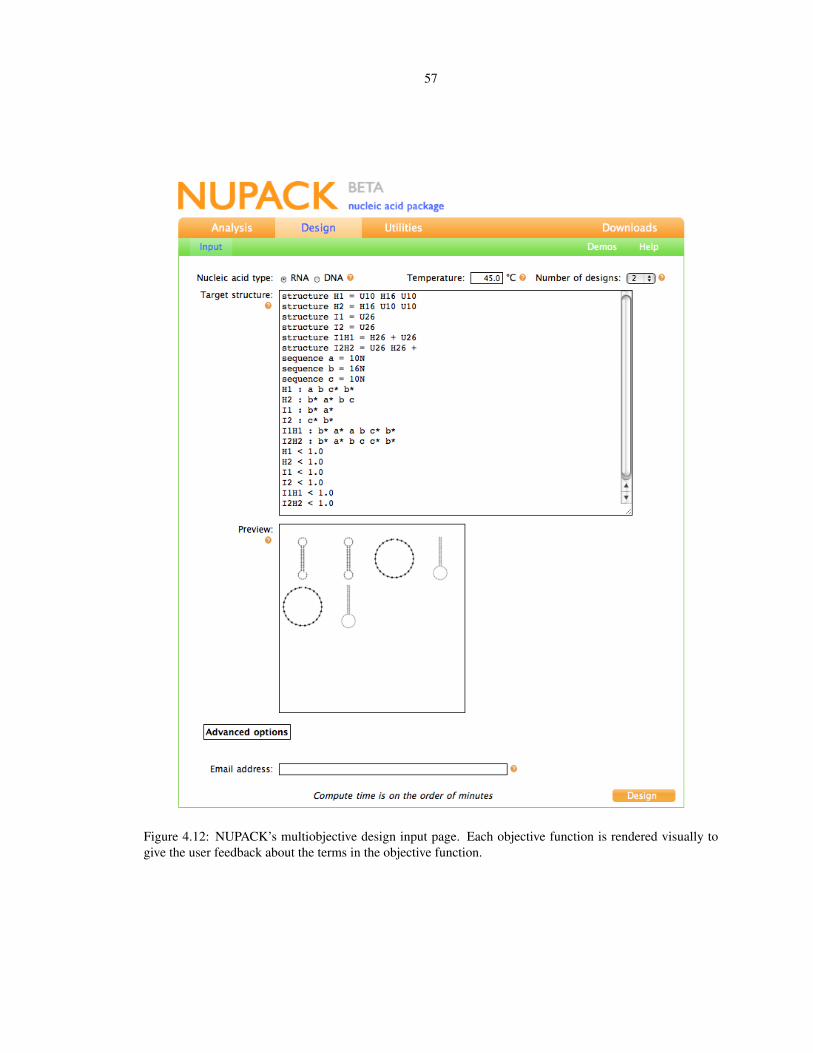
57
Figure 4.12: NUPACK’s multiobjective design input page. Each objective function is rendered visually togive the user feedback about the terms in the objective function.

58
Figure 4.13: NUPACK’s design results detail page for multiobjective design, listing unique strands thatcomprise the system.

59
Figure 4.14: NUPACK’s design results detail page for multiobjective design.

60
cloned, in a scaled-down verison, into a test cluster. This allows us to test new features without disturbing the
live, public version of the site.
The web server handles all user requests. If a calculation or drawing predicted to take less than a second
is requested, the computation will execute directly on the cluster head node. Longer computation is broken
down into a directed acyclic graph of component subjobs. The head node will then submit these subjobs
to the cluster in the appropriate order. If a subjob is predicted to take less than a minute and use a single
processor, it will run on the cluster nodes designated for fast jobs. If it is predicted to take more than a minute
or use multiple processors, the job will run on the nodes designated for long jobs. Queues are used to provide
efficient utilization of resources.
The compute cluster, head node, and web server all have access to the same file system. This allows
the web server to easily send rendered image files to the user upon request. The web server and head node
also have access to a relational database, which stores important numeric and sequence results that can be
displayed to the user or exported into other modules.
The NUPACK web application is programmed within the Ruby on Rails framework, employing AJAX
and the Dojo Toolkit to implement dynamic features and interactive graphics. The NUPACK library of
analysis and design algorithms is written in the C and C++ programming language. Dynamic programs are
parallelized using MPI [26]. The Ruby and Python languages are also used for plot drawing and back-end
data aggregation. Further implementation details including software are given in Appendix A.
NUPACK’s front end is designed to be compatible with the current versions of three popular, freely
available browsers: Firefox, Safari, and Chrome. Other compatible browsers must support XHTML,
CSS, SVG, Javascript, and the use of cookies. All vector images are stored in the SVG format. All raster
images are stored in the PNG format.
NUPACK officially launched its beta version of the Analysis module on Feburary 1, 2007. A beta version
of single-complex design was launched on March 1, 2007. All three modules were officially released on
January 10, 2010. At this same time, the multiobjective design capability was released as private beta to
members of the Molecular Programming Project at Caltech and University of Washington. Usage statistics
are provided in Appendix E.

61
Chapter 5
Summary and outlook
This thesis focuses on making thermodynamic nucleic acid design a high-quality, versatile, and low-cost
technology that is easy to use and easily accessible. We demonstrated how to achieve high-quality sequences
via ensemble defect optimization for only 4/3 the cost of the objective function for large structures. We have
further increased design versatility by developing an algorithm for the design of multi-state systems of nucleic
acids that also achieves high-quality sequence for low cost with ensemble defect optimization. Finally, we
have presented a web server that makes parallel implementations of these and other algorithms easy to use
and accessible with the use of a specialized front-end to a high-performance compute cluster. The highly
interactive features and visualization tools of NUPACK allow for users to explore and communicate their
results with greater understanding and further reach than was previously possible. Nevertheless, improving
cost, scope, and availability remains an open area of research.
5.1 Computational cost
Even though our single-complex design algorithm is performing near the optimum, improvements in how our
objective function implementations interact with underlying hardware architecture could potentially lower
computational cost. The current implementations of the Θ(N3) algorithms interact with memory in such
a way that they prevent concurrent processes from efficiently sharing. Implementing the objective function
algorithms to utilize improved memory access synchronization methods would allow for better concurrent
performance. Furthermore, vectorizing the partition function and probability matrix calculations such that
they could run efficiently on a SIMD processor would allow for the utilization of newer and cheaper architec-
tures such as GPUs. Some areas of scientific research such as molecular dynamics have experienced speed
gains of over two order of magnitude by utilizing these architectures [60]. Furthermore, NUPACK currently
stores floating point values with 128 bits on a 64-bit system in order to capture the dynamic range of the par-
tition function. Modifying the algorithms to perform calculations with values stored in double precision (i.e.,
64 bits) would not only improve performance but would also open doors to other specialized architectures.
Improved resource management could also allow for more efficient designs. The algorithms presented in

62
this thesis may benefit from designing multiple unlinked leaves of a decomposition tree simultaneously. The
challenge lies in that subproblem complexities are heterogeneous, making it difficult to preallocate resources
such that processors are efficiently used. More sophisticated resource management would allow many differ-
ent designs by different users to be computed simultaneously, such that they use and release processors from
a pool as necessary. The multi-state algorithm presented in Chapter 3 was implemented with grid comput-
ing architectures in mind (i.e., the global sequence table can be stored in a master lightweight process that
synchronizes multiple independent design processes).
5.2 Design versatility
In Chapter 3 we demonstrated that certain systems from literature are difficult to design, often a result of re-
duced sequence space or specified structures incompatible with the parameters for the energy model. While
this could be addressed by the engineer studying resulting pair probability matrices and manually redimen-
sioning some structural elements [45], it would be advantageous to have the tools to perform this specification
optimization automatically. Shrinking a structure while maintaining function could improve fabrication costs,
while adding more stability to some structural elements could improve experimental performance.
Our current multi-state algorithm does not take into account the concentration of each individual strand
in the system. Designing strands to form a complex with high affinity and specificity does not guarantee that
they will form with desired concentration in a dilute solution. The ability to design strands to form with the
correct concentrations at equilibrium will also be useful to prevent certain species from interacting with each
other (i.e., certain complexes are assigned a zero target concentration).
We have studied the performance of our algorithms in the context of empirical secondary structure free
energy models [10, 11] that have practical utility for the analysis [36–40] and design [41–46] of functional
nucleic acid systems. It would also be beneficial to develop a set of experiments that study the accuracy of
NUPACK’s predictions. Furthermore, work in the area of kinetic analysis and rational kinetic design will be
of great utility for designing and analyzing nucleic acid systems.
5.3 Availability
In addition to providing tools to the research community, making our work available over the web has pro-
vided very valuable insight through continuous feedback from our users. This feedback helps inform us
of desired features and tools. Continuously improving the site’s performance will inevitably lead to better
technological development.

63
5.4 A compiler for biomolecular function
The advancement of computer science has led to the construction of highly complex electronic systems
with billions of interacting components. To reach this state, researchers developed tools and languages for
obscuring this complexity into higher levels of abstraction. Since the field of nucleic acid nanotechnology is
built on the notion that nucleic acids are fundamentally programmable, it follows that we should be able to
build similar tools for molecular programming.
Traditional compilers translate programs from one language into another, usually from high- to low-level
languages [61]. A compiler for biomolecular function would similarly allow users to specify abstract func-
tions and concepts without concerning themselves with the underlying molecular representations. While there
remains much work to be done before a molecular compiler functions with the reliability of its silicon analog,
the work presented in this thesis has attempted to address issues related to the lower layers of compilation:
programming equilibrium secondary structure into primary sequence. This thesis also demonstrates that the
web will be a very compelling platform for distributing molecular programming tools.
64
Bibliography
[1] B. Alberts, et al., Molecular Biology of the Cell (Garland Science, New York, 2002), 4th ed.
[2] M. H. Caruthers, Gene synthesis machines: DNA chemistry and its uses, Science 230, 281-285 (1985).
[3] N. Seeman, Nucleic acid junctions and lattices, J. Theor. Biol. 99, 237-247 (1982).
[4] F. Simmel, W. Dittmer, DNA nanodevices, Small 1, 284-299 (2005).
[5] U. Feldkamp, C. Niemeyer, Rational design of DNA nanoarchitectures, Angewandte Chemie Interna-
tional Edition 45, 1856-1876 (2006).
[6] U. Feldkamp, C. M. Niemeyer, Rational engineering of dynamic DNA systems, Angewandte Chemie-
International Edition 47, 3871-3873 (2008).
[7] J. Bath, A. Turberfield, DNA nanomachines, Nature Nanotechnology 2, 275-284 (2007).
[8] R. Dirks, J. Bois, J. Schaeffer, E. Winfree, N. Pierce, Thermodynamic analysis of interacting nucleic
acid strands, SIAM Review 49, 65-88 (2007).
[9] M. Serra, D. Turner, Predicting thermodynamic properties of RNA, Methods Enzymol 259, 242-261
(1995).
[10] D. Mathews, J. Sabina, M. Zuker, D. Turner, Expanded sequence dependence of thermodynamic pa-
rameters improves prediction of RNA secondary structure, Journal of Molecular Biology 288, 911-940
(1999).
[11] J. SantaLucia, Jr., A unified view of polymer, dumbbell, and oligonucleotide DNA nearest-neighbor
thermodynamics, Proceedings of the National Academy of Sciences of the United States of America 95,
1460-1465 (1998).
[12] J. SantaLucia, D. Hicks, The thermodynamics of DNA structural motifs, Annu Rev Bioph Biom 33,
415-440 (2004).
[13] R. Koehler, N. Peyret, Thermodynamic properties of DNA sequences: characteristic values for the
human genome, Bioinformatics 21, 3333-3339 (2005).
65
[14] V. Bloomfield, D. Crothers, I. Tinoco, Jr., Nucleic Acids: Structures, Properties, and Functions (Uni-
versity Science Books, Sausalito, CA, 2000).
[15] I. Tinoco, Jr., O. Uhlenbeck, M. Levine, Estimation of secondary structure in ribonucleic acids, Nature
230, 362-367 (1971).
[16] M. Zuker, P. Stiegler, Optimal computer folding of large RNA sequences using thermodynamics and
auxiliary information, Nucleic Acids Res 9, 133-147 (1981).
[17] L. Landau, E. Lifshitz, Statistical Physics Part 1 (Butterworth-Heinemann, New York, 1980), 3rd ed.
[18] M. Zuker, D. Sankoff, RNA secondary structures and their prediction, Bulletin of Mathematical Biology
46, 591-621 (1984).
[19] J. McCaskill, The equilibrium partition function and base pair binding probabilities for RNA secondary
structure, Biopolymers 29, 1105-1119 (1990).
[20] I. Hofacker, et al., Fast folding and comparison of RNA secondary structures, Chemical Monthly 125,
167-188 (1994).
[21] R. Lyngsø, M. Zuker, C. Pedersen, Fast evaluation of internal loops in RNA secondary structure predic-
tion, Bioinformatics 15, 440-445 (1999).
[22] R. Dirks, N. Pierce, An algorithm for computing nucleic acid base-pairing probabilities including pseu-
doknots, Journal of Computational Chemistry 25, 1295-1304 (2004).
[23] R. Dimitrov, M. Zuker, Prediction of hybridization and melting for double-stranded nucleic acids, Bio-
physical Journal 87, 215-226 (2004).
[24] M. Andronescu, Z. Zhang, A. Condon, Secondary structure prediction of interacting RNA molecules,
Journal of Molecular Biology 345, 987-1001 (2005).
[25] S. Bernhart, et al., Partition function and base pairing probabilities of RNA heterodimers, Algorithms
for Molecular Biology 1, 3 (2006).
[26] M. Fekete, I. Hofacker, P. Stadler, Prediction of RNA base pairing probabilities on massively parallel
computers, Journal of Computational Biology 7, 171-182 (2000).
[27] M. Andronescu, A. Fejes, F. Hutter, H. Hoos, A. Condon, A new algorithm for rna secondary structure
design, Journal of Molecular Biology 336, 607-624 (2004).
[28] A. Busch, R. Backofen, INFO-RNA–a fast approach to inverse RNA folding, Bioinformatics 22, 1823-
1831 (2006).
66
[29] R. Aguirre-Hernandez, H. Hoos, A. Condon, Computational RNA secondary structure design: Ehoosm-
pirical complexity and improved methods, BMC Bioinformatics 8, Article 34 (2007).
[30] B. Burghardt, A. Hartmann, RNA secondary structure design, Physical Review E 75, 021920 (2007).
[31] R. Dirks, M. Lin, E. Winfree, N. Pierce, Paradigms for computational nucleic acid design, Nucleic Acids
Res 32, 1392-1403 (2004).
[32] C. Flamm, I. Hofacker, S. Maurer-Stroh, P. Stadler, M. Zehl, Design of multistable RNA molecules,
RNA 7, 254-265 (2001).
[33] R. Dirks, N. Pierce, A partition function algorithm for nucleic acid secondary structure including pseu-
doknots, Journal of Computational Chemistry 24, 1664-1677 (2003).
[34] H. Hoos, T. Stutzle, Stochastic Local Search: Foundations and Applications (Morgan Kaufmann, 2005).
[35] B. R. Wolfe, Personal communication (2009).
[36] Y. Ding, C. Lawrence, A statistical sampling algorithm for RNA secondary structure prediction, Nucleic
Acids Res 31, 7280-7301 (2003).
[37] D. Mathews, Using an RNA secondary structure partition function to determine confidence in base pairs
predicted by free energy minimization, RNA 10, 1178-1190 (2004).
[38] Y. Ding, C. Chan, C. Lawrence, RNA secondary structure prediction by centroids in a Boltzmann
weighted ensemble, RNA 11, 1157-1166 (2005).
[39] S. Rogic, et al., Correlation between the secondary structure of pre-mRNA introns and the efficiency of
splicing in saccharomyces cerevisiae, BMC Genomics 9, 355 (2008).
[40] J. Zhi, J. Gloor, D. Mathews, Improved RNA secondary structure prediction by maximizing expected
pair accuracy, RNA 15, 1805-1813 (2009).
[41] R. Dirks, N. Pierce, Triggered amplification by hybridization chain reaction, Proceedings of the Na-
tional Academy of Sciences of the United States of America 101, 15275-15278 (2004).
[42] V. Patzel, et al., Design of siRNAs producing unstructured guide-RNAs results in improved RNA inter-
ference efficiency, Nature Biotechnology 23, 1440-1444 (2005).
[43] R. Penchovsky, R. Breaker, Computational design and experimental validation of oligonucleotide-
sensing allosteric ribozymes, Nature Biotechnology 23, 1424-1433 (2005).
[44] S. Venkataraman, R. Dirks, P. Rothemund, E. Winfree, N. Pierce, An autonomous polymerization motor
powered by dna hybridization, Nature Nanotechnology 2, 490-494 (2007).

67
[45] P. Yin, H. Choi, C. Calvert, N. Pierce, Programming biomolecular self-assembly pathways, Nature 451,
318-322 (2008).
[46] H. Choi, et al., Programmable in situ amplification for multiplexed bioimaging. in review .
[47] G. Seelig, D. Soloveichik, D. Zhang, E. Winfree, Enzyme-free nucleic acid logic circuits, Science 314,
1585-1588 (2006).
[48] M. Zuker, Mfold web server for nucleic acid folding and hybridization prediction, Nucleic Acids Res
31, 3406-3415 (2003).
[49] N. Markham, M. Zuker, UNAFold: Software for nucleic acid folding and hybridization., Methods in
molecular biology (Clifton, NJ) 453, 3 (2008).
[50] A. Gruber, R. Lorenz, S. Bernhart, R. Neubock, I. Hofacker, The vienna RNA websuite, Nucleic acids
research 36, W70 (2008).
[51] N. Markham, M. Zuker, DINAMelt web server for nucleic acid melting prediction, Nucleic Acids Res
33, W577 (2005).
[52] M. Andronescu, R. Aguirre-Hernandez, A. Condon, H. H. Hoos, Rnasoft: A suite of rna secondary
structure prediction and design software tools, Nucleic Acids Res 31, 3416–22 (2003).
[53] A. Busch, R. Backofen, INFO-RNA - a server for fast inverse RNA folding satisfying sequence con-
straints, Nucleic Acids Res 35, W310–W313 (2007).
[54] G. Lapalme, R. Cedergren, D. Sankoff, An algorithm for the display of nucleic acid secondary structure.,
Nucleic Acids Res 10, 8351 (1982).
[55] B. Shapiro, L. Lipkin, J. Maizel, An interactive technique for the display of nucleic acid secondary
structure, Nucleic Acids Res 10, 7041 (1982).
[56] B. Shapiro, J. Maizel, L. Lipkin, K. Currey, C. Whitney, Generating non-overlapping displays of nucleic
acid secondary structure, Nucleic acids research 12, 75–88 (1984).
[57] R. Bruccoleri, G. Heinrich, An improved algorithm for nucleic acid secondary structure display, Bioin-
formatics 4, 167 (1988).
[58] P. De Rijk, J. Wuyts, R. De Wachter, RnaViz 2: an improved representation of RNA secondary structure,
Bioinformatics 19, 299 (2003).
[59] K. Darty, A. Denise, Y. Ponty, VARNA: Interactive drawing and editing of the RNA secondary structure,
Bioinformatics 25, 1974 (2009).

68
[60] M. Friedrichs, et al., Accelerating molecular dynamic simulation on graphics processing units, Journal
of Computational Chemistry 30, 864–872 (2009).
[61] A. Aho, R. Sethi, J. Ullman, Compilers, Principles, Techniques, and Tools (Addison Wesley Publishing
Company, 1986).
[62] L. Qian, E. Winfree, A simple DNA gate motif for synthesizing large-scale circuits, DNA Computing
pp. 70–89 (2009).
[63] S. Ligocki, C. Berlind, Personal communication (2009).
[64] M. Schwarzkopf, Personal communication (2009).

69
Appendix A
Computing resources, languages, andsoftware dependencies
A.1 Cluster hardware resources
Model Cores Clock Speed (GHz) Cache Size (MB)A Intel® Xeon® E5540 4 2.53 8B Intel® Xeon® E5530 4 2.40 8C Intel® Xeon® E5345 2 2.33 8
Table A.1: CPU details
Cluster Node Type Node Count Node RAM (GB) CPUs Total Cores
NUPACKWebserver 1 24 A×2 8
Head 1 24 B×2 8Compute 30 24 A×2 240
TestWebserver 1 24 A×2 8
Head 1 24 A×2 8Compute 1 24 A×2 8
Development Head 1 48 B×2 8Compute 16 4 C×2 64
Table A.2: Summary of compute cluster resources. The CPU types are crossreferenced with Table A.1
All computing, development, and production run on 64-bit Intel® Xeon® processors with attributes de-
scribed in Table A.1. Resources are divided into the following three clusters, all with TCP/IP networking
over Gigabit Ethernet:
NUPACK Cluster : This is the hardware that runs the live version of NUPACK.org. It is also the cluster
used for final timing results.
Test Cluster : The NUPACK web application is developed on this cluster with production quality algorithms
running on the worker node. New features are tested in a production environment before deploying to

70
the live server.
Development Cluster : Algorithms are developed and tested on this cluster.
The properties of each cluster are defined in Table A.2.
A.2 Languages
C : all NUPACK energy calculations, concentration solver, single-complex designer, single-complex test-
suite generator, test-suite structure analyzer
C++ : multiobjective designer
Ruby 1.8 : all webserver code
Python 2.4 : secondary structure drawing, pair probability plotting, multiobjective input parsing
JavaScript : used for interactive web features
SVG : all vector images generated by NUPACK are in this open format
XHTML : the format of all web pages served by NUPACK
A.3 Software dependencies
Cluster and resource management
Rocks 5.2 Chimichanga (http://www.rocksclusters.org): Linux distribution designed for
scientific clusters.
Open MPI (http://www.open-mpi.org/): implementation of the MPI-2 message passing standard
for parallel computing.
Torque Resource Manager (http://www.clusterresources.com/products/torque-resource-manager.
php): software responsible for allocating computational resources.
Maui (http://www.clusterresources.com/products/maui-cluster-scheduler.php/):
software used in conjunction with Torque to schedule computational jobs.
Compilers and development tools
GNU Compiler Collection (http://gcc.gnu.org): Collection of compilers and debugging tools.
71
Intel® Compiler Suite (http://software.intel.com/en-us/intel-compilers/): A
compiler with special optimizations for Intel® processors.
Subversion (http://subversion.tigris.org/): Revision control system.
Valgrind (http://valgrind.org/): tools for debugging and profiling executable code.
Libraries
JsonCpp (http://jsoncpp.sourceforge.net/): A C++ library for reading and writing data in
the JavaScript Object Notation (JSON format).
Mersenne Twister (http://www.math.sci.hiroshima-u.ac.jp/˜m-mat/MT/emt.html):
Platform-independent, high-quality random number generator.
Drawing
LAPACK (http://www.netlib.org/lapack/): Linear Algebra PACKage.
BLAS (http://www.netlib.org/blas/): Basic Linear Algebra Subprograms.
matplotlib (http://matplotlib.sourceforge.net/): Python plotting library designed to re-
semble MATLAB.
NumPy (http://numpy.scipy.org/): Python extension for handling numerical operations on large
arrays and matrices
SciPy (http://www.scipy.org): Python library of algorithms and mathematical tools
librsvg (http://librsvg.sourceforge.net/): SVG rendering library
ImageMagick (http://www.imagemagick.org): Software suite for converting images from one
format to another.
GLE (http://glx.sourceforge.net/): A scripting language for creating graphs and plots.
OpenGL (http://www.opengl.org/): API for producing 2D and 3D graphics.
Web development
Ruby on Rails (http://rubyonrails.org/): web application framework for Ruby
PostgreSQL (http://www.postgresql.org/): object-relational database management system
Apache Qpid (http://qpid.apache.org/): messaging system that implements the Advanced Mes-
sage Queueing Protocol.

72
Dojo Toolkit (http://www.dojotoolkit.org/): JavaScript library for developing rich web ap-
plications.
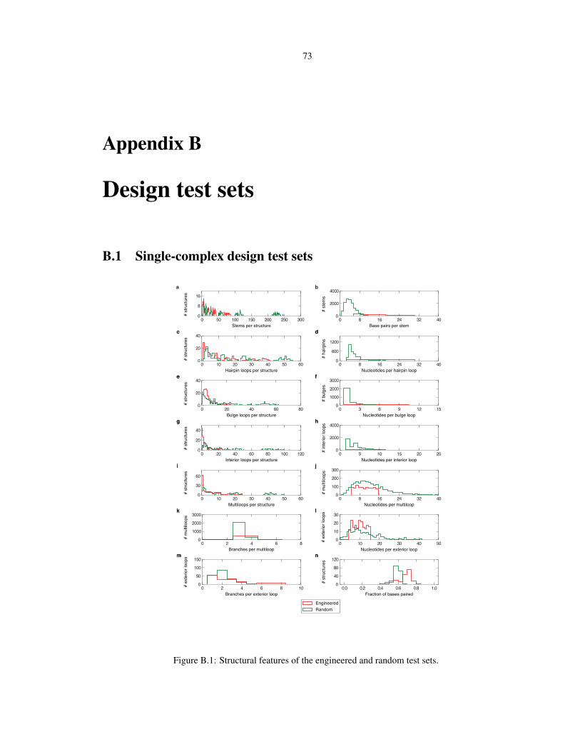
73
Appendix B
Design test sets
B.1 Single-complex design test sets
0 50 100 150 200 250 300Stems per structure
0
8
16
# str
uctu
res
0 8 16 24 32 40Base pairs per stem
0
2000
4000
# ste
ms
0 10 20 30 40 50 60Hairpin loops per structure
0
20
40
# str
uctu
res
0 8 16 24 32 40Nucleotides per hairpin loop
0
600
1200
# ha
irpins
0 20 40 60 80Bulge loops per structure
0
20
40
# str
uctu
res
0 3 6 9 12 15Nucleotides per bulge loop
0100020003000
# bu
lges
0 20 40 60 80 100 120Interior loops per structure
0
20
40
# str
uctu
res
0 5 10 15 20 25Nucleotides per interior loop
0
2000
4000
# int
erior
loop
s
0 10 20 30 40 50 60Multiloops per structure
0
30
60
# str
uctu
res
0 8 16 24 32 40Nucleotides per multiloop
0100200300
# m
ultilo
ops
0 2 4 6 8Branches per multiloop
0100020003000
# m
ultilo
ops
0 2 4 6 8 10Branches per exterior loop
050
100150
# ex
terio
r loo
ps
0 10 20 30 40 50Nucleotides per exterior loop
0102030
# ex
terio
r loo
ps
0.0 0.2 0.4 0.6 0.8 1.0Fraction of bases paired
04080
120
# str
uctu
res
EngineeredRandom
a b
mm nn
kk ll
ii jj
gg hh
ee ff
cc dd
Figure B.1: Structural features of the engineered and random test sets.

74
B.2 Multiobjective design test suite
structure H1 = U6 H18 (U6)structure H2 = H18 (U6) U6structure I = U24structure I H1 = H24 (U24 +)structure I H1 H2 = H24 (H24 (+ U24) +)sequence a = 6Nsequence b = 18Nsequence c = 6NH1 : a b c b*H2 : b* a* b c*I : b* a*I H1 : a b c b* b* a*I H1 H2 : a b c b* b* a* b c* b* a*H1 < 1.0H2 < 1.0I < 1.0I H1 < 1.0I H1 H2 < 1.0
Figure B.2: Code for hybridization chain reaction [41]. This system is designed with DNA energy parametersat 23 C.

75
structure H1 = U6 H18 (U6) U3structure H2 = U3 H18 (U6) U6structure AR = H18 (U6 + U3) U3structure State2 = H24 (U6 H21 (+) U3 +)structure State4 = H24 (H24 (H3 (+) H21 (+) U6) +)sequence a = 6Nsequence b = 18Nsequence c = 6Nsequence x = 3Nsequence y = 3NH1 : a b c b* x*H2 : y* b* a* b c*AR : b* a* x b yState2 : a b c b* x* x b y b* a*State4 : a b c b* x* x b y y* b* a* b c* b* a*H1 < 1.0H2 < 1.0AR < 1.0State2 < 1.0State4 < 1.0
Figure B.3: Synthetic molecular motor inspired by Rickettsia rickettsii [44]. This system is designed withDNA energy parameters at 23 C.
structure G-Eout-F = H15(U27 H15(H30(U6 +)))structure Gin = U36structure Fin = U36structure G-Gin = H36 (+)structure Eout-F = H15(U27 H15(+ U30))structure Eout = U57structure Fin-F = H36(+ U24)sequence Gtoe = 6Nsequence Ftoe = 6Nsequence G = 24Nsequence F1 = 15Nsequence F2 = 15Nsequence E = 27NG-Eout-F : F1 E F2 Ftoe* G Gtoe G* Ftoe F2* F1*Gin : Gtoe* G* FtoeFin : F2 F1 Ftoe*G-Gin : Ftoe* G Gtoe Gtoe* G* FtoeEout-F : F1 E F2 G* Ftoe F2* F1*Eout : F2 E F1Fin-F : F2 F1 Ftoe* G* Ftoe F2* F1*G-Eout-F < 1.0Gin < 1.0Fin < 1.0G-Gin < 1.0Eout-F < 1.0Fin-F < 1.0
Figure B.4: Code for 2-input And logic gate [47]. This system is designed with DNA energy parameters at23 C.
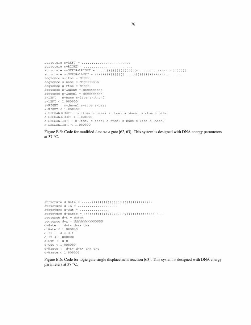
76
structure s-LEFT = .........................structure s-RIGHT = .........................structure s-SEESAW RIGHT = .....(((((((((((((((+..........)))))))))))))))structure s-SEESAW LEFT = (((((((((((((((.....+)))))))))))))))..........sequence s-ltoe = NNNNNsequence s-base = NNNNNNNNNNsequence s-rtoe = NNNNNsequence s- Anon0 = NNNNNNNNNNsequence s- Anon1 = NNNNNNNNNNs-LEFT : s-base s-ltoe s- Anon0s-LEFT < 1.000000s-RIGHT : s- Anon1 s-rtoe s-bases-RIGHT < 1.000000s-SEESAW RIGHT : s-ltoe* s-base* s-rtoe* s- Anon1 s-rtoe s-bases-SEESAW RIGHT < 1.000000s-SEESAW LEFT : s-ltoe* s-base* s-rtoe* s-base s-ltoe s- Anon0s-SEESAW LEFT < 1.000000
Figure B.5: Code for modified Seesaw gate [62, 63]. This system is designed with DNA energy parametersat 37 C.
structure d-Gate = .....(((((((((((((((+)))))))))))))))structure d-In = ....................structure d-Out = ...............structure d-Waste = ((((((((((((((((((((+))))))))))))))))))))sequence d-t = NNNNNsequence d-x = NNNNNNNNNNNNNNNd-Gate : d-t* d-x* d-xd-Gate < 1.000000d-In : d-x d-td-In < 1.000000d-Out : d-xd-Out < 1.000000d-Waste : d-t* d-x* d-x d-td-Waste < 1.000000
Figure B.6: Code for logic gate single displacement reaction [63]. This system is designed with DNA energyparameters at 37 C.
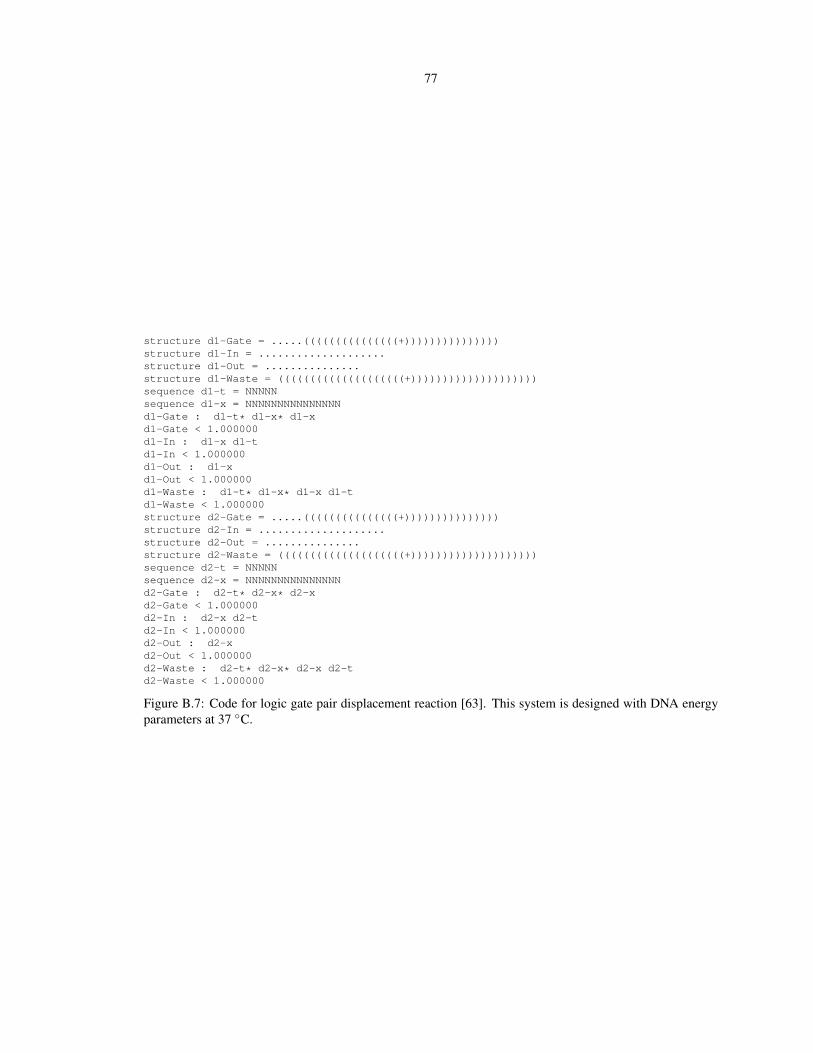
77
structure d1-Gate = .....(((((((((((((((+)))))))))))))))structure d1-In = ....................structure d1-Out = ...............structure d1-Waste = ((((((((((((((((((((+))))))))))))))))))))sequence d1-t = NNNNNsequence d1-x = NNNNNNNNNNNNNNNd1-Gate : d1-t* d1-x* d1-xd1-Gate < 1.000000d1-In : d1-x d1-td1-In < 1.000000d1-Out : d1-xd1-Out < 1.000000d1-Waste : d1-t* d1-x* d1-x d1-td1-Waste < 1.000000structure d2-Gate = .....(((((((((((((((+)))))))))))))))structure d2-In = ....................structure d2-Out = ...............structure d2-Waste = ((((((((((((((((((((+))))))))))))))))))))sequence d2-t = NNNNNsequence d2-x = NNNNNNNNNNNNNNNd2-Gate : d2-t* d2-x* d2-xd2-Gate < 1.000000d2-In : d2-x d2-td2-In < 1.000000d2-Out : d2-xd2-Out < 1.000000d2-Waste : d2-t* d2-x* d2-x d2-td2-Waste < 1.000000
Figure B.7: Code for logic gate pair displacement reaction [63]. This system is designed with DNA energyparameters at 37 C.

78
structure A = U4 H14 U18structure B = U4 H16 U14structure C = U4 H24 U14structure T = U20structure TA = H20 (U30+)structure SA B = H22 (U28+)structure BC = H48 (U2 +) U18structure SA = U22structure SB = U28structure SC = U18structure toeA = U4structure toeB = U4structure toeC = U4structure loopA = U18structure loopB = U14structure loopC = U14structure overx = U2structure openC = U38sequence a = 4Nsequence c = 4Nsequence x = 2Nsequence y = 10Nsequence d = 8Nsequence m = 8Nsequence s = 2Nsequence t = 4NA: t m a x s x y* c* x* a* m*B: a x c y x* a* d* y* c* x*C: c y d a x y* c* x* a* d* y*T: s* x* a* m* t*TA: t m a x s x y* c* x* a* m* s* x* a* m* t*SA B: a x c y x* a* d* y* c* x* x y* c* x* a*BC: a x c y x* a* d* y* c* x* c y d a x y* c* x* a* d* y*SA: x y* c* x* a*SB: a* d* y* c* x*SC: d* y*toeA: ttoeB: atoeC: cloopA: s x y* c*loopB: x* a* d*loopC: y* c*overx: x*openC: y* c* x* a* d* y*A<1.0B<1.0C<1.0T<1.0TA<1.0SA B<1.0BC<1.0SA<1.0SB<1.0SC<1.0toeA<1.0toeB<1.0toeC<1.0loopA<1.0loopB<1.0loopC<1.0openC<1.0overx<1.0
Figure B.8: Code for test tube Dicer system [64]. This system is designed with RNA energy parameters at 37C.

79
Appendix C
Pseudocode for other single-complexdesign algorithms
DESIGNSEQ(s)
mleafopt ← 0φ, n← OPTIMIZELEAF(s)while n > fstop|s| and mleafopt < Mleafopt
φ, n← OPTIMIZELEAF(s)if n < n
φ, n← φ, nmleafopt ← mleafopt + 1
return φ
OPTIMIZELEAF(s)
munfavorable ← 0γunfavorable ← ∅φ← INITSEQ(s)n← ENSEMBLEDEFECT(φ, s)while n > fstop|s| and munfavorable < Munfavorable|s|
ξ, φ← UNIFORMMUTATIONSAMPLING(φ, s)if ξ ∈ γunfavorable
munfavorable ← munfavorable + 1else
n← ENSEMBLEDEFECT(φ, s)if n < n
φ, n← φ, nmunfavorable ← 0γunfavorable ← ∅
elsemunfavorable ← munfavorable + 1γunfavorable ← γunfavorable ∪ ξ
return φ, n
Algorithm C.1: Single-scale ensemble defect optimization with uniform mutation sampling.

80
DESIGNSEQ(s)
mleafopt ← 0φ, n← OPTIMIZELEAF(s)while n > fstop|s| and mleafopt < Mleafopt
φ, n← OPTIMIZELEAF(φ, s)if n < n
φ, n← φ, nmleafopt ← mleafopt + 1
return φ
OPTIMIZELEAF(s)
munfavorable ← 0γunfavorable ← ∅φ← INITSEQ(s)n← ENSEMBLEDEFECT(φ, s)while n > fstop|s| and munfavorable < Munfavorable|s|
ξ, φ← WEIGHTEDMUTATIONSAMPLING(φ, s, n1, . . . , n|s|)if ξ ∈ γunfavorable
munfavorable ← munfavorable + 1else
n← ENSEMBLEDEFECT(φ, s)if n < n
φ, n← φ, nmunfavorable ← 0γunfavorable ← ∅
elsemunfavorable ← munfavorable + 1γunfavorable ← γunfavorable ∪ ξ
return φ, n
Algorithm C.2: Single-scale ensemble defect optimization with defect-weighted mutation sampling.
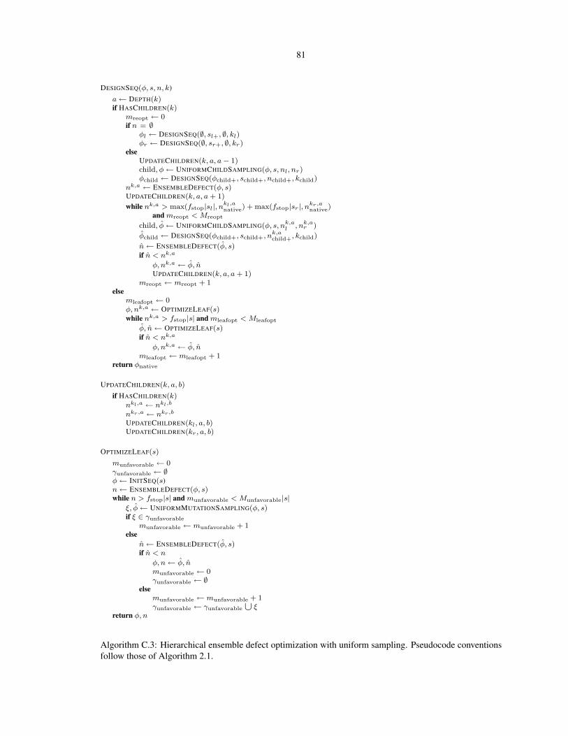
81
DESIGNSEQ(φ, s, n, k)
a← DEPTH(k)if HASCHILDREN(k)
mreopt ← 0if n = ∅
φl ← DESIGNSEQ(∅, sl+, ∅, kl)φr ← DESIGNSEQ(∅, sr+, ∅, kr)
elseUPDATECHILDREN(k, a, a− 1)child, φ← UNIFORMCHILDSAMPLING(φ, s, nl, nr)φchild ← DESIGNSEQ(φchild+, schild+, nchild+, kchild)
nk,a ← ENSEMBLEDEFECT(φ, s)UPDATECHILDREN(k, a, a+ 1)
while nk,a > max(fstop|sl|, nkl,anative) + max(fstop|sr|, nkr,a
native)and mreopt < Mreopt
child, φ← UNIFORMCHILDSAMPLING(φ, s, nk,al , nk,a
r )
φchild ← DESIGNSEQ(φchild+, schild+, nk,achild+, kchild)
n← ENSEMBLEDEFECT(φ, s)if n < nk,a
φ, nk,a ← φ, nUPDATECHILDREN(k, a, a+ 1)
mreopt ← mreopt + 1else
mleafopt ← 0φ, nk,a ← OPTIMIZELEAF(s)while nk,a > fstop|s| and mleafopt < Mleafopt
φ, n← OPTIMIZELEAF(s)if n < nk,a
φ, nk,a ← φ, nmleafopt ← mleafopt + 1
return φnative
UPDATECHILDREN(k, a, b)
if HASCHILDREN(k)nkl,a ← nkl,b
nkr,a ← nkr,b
UPDATECHILDREN(kl, a, b)UPDATECHILDREN(kr, a, b)
OPTIMIZELEAF(s)
munfavorable ← 0γunfavorable ← ∅φ← INITSEQ(s)n← ENSEMBLEDEFECT(φ, s)while n > fstop|s| and munfavorable < Munfavorable|s|
ξ, φ← UNIFORMMUTATIONSAMPLING(φ, s)if ξ ∈ γunfavorable
munfavorable ← munfavorable + 1else
n← ENSEMBLEDEFECT(φ, s)if n < n
φ, n← φ, nmunfavorable ← 0γunfavorable ← ∅
elsemunfavorable ← munfavorable + 1γunfavorable ← γunfavorable ∪ ξ
return φ, n
Algorithm C.3: Hierarchical ensemble defect optimization with uniform sampling. Pseudocode conventionsfollow those of Algorithm 2.1.

82
DESIGNSEQ(s)
mleafopt ← 0φ, π ← OPTIMIZELEAF(s)while π > fstop and mleafopt < Mleafopt
φ, π ← OPTIMIZELEAF(s)if π < π
φ, π ← φ, πmleafopt ← mleafopt + 1
return φ
OPTIMIZELEAF(s)
munfavorable ← 0γunfavorable ← ∅φ← INITSEQ(s)π ←PROBABILITYDEFECT(φ, s)while π > fstop and munfavorable < Munfavorable|s|
ξ, φ← UNIFORMMUTATIONSAMPLING(φ, s)if ξ ∈ γunfavorable
munfavorable ← munfavorable + 1else
π ←PROBABILITYDEFECT(φ, s)if π < π
φ, π ← φ, πmunfavorable ← 0γunfavorable ← ∅
elsemunfavorable ← munfavorable + 1γunfavorable ← γunfavorable ∪ ξ
return φ, π
Algorithm C.4: Single-scale probability defect optimization with uniform mutation sampling.

83
DESIGNSEQ(φ, s, µ, k)a← DEPTH(k)if HASCHILDREN(k)
mreopt ← 0if µ = ∅
φl ← DESIGNSEQ(∅, sl+, ∅, kl)φr ← DESIGNSEQ(∅, sr+, ∅, kr)
elseUPDATECHILDREN(k, a, a− 1)child, φ← WEIGHTEDCHILDSAMPLING(φ, s, µl, µr)φchild ← DESIGNSEQ(φchild+, schild+, µchild+, kchild)
µk,a ← MFEDEFECT(φ, s)UPDATECHILDREN(k, a, a+ 1)
while µk,a > max(fstop|sl|, µkl,a
native) + max(fstop|sr|, µkr,anative)
andmreopt < Mreopt
µi ← µk,ai + ε ∀i ∈ 1, . . . , |s|
child, φ← WEIGHTEDCHILDSAMPLING(φ, s, µl, µr)
φchild ← DESIGNSEQ(φchild+, schild+, µchild+, kchild)
µ← MFEDEFECT(φ, s)
if µ < µk,a
φ, µk,a ← φ, µUPDATECHILDREN(k, a, a+ 1)
mreopt ← mreopt + 1else
mleafopt ← 0
φ, µk,a ← OPTIMIZELEAF(s)
while µk,a > fstop|s| andmleafopt < Mleafopt
φ, µ← OPTIMIZELEAF(s)
if µ < µk,a
φ, µk,a ← φ, µmleafopt ← mleafopt + 1
return φnative
UPDATECHILDREN(k, a, b)
if HASCHILDREN(k)
µkl,a ← µkl,b
µkr,a ← µkr,b
UPDATECHILDREN(kl, a, b)UPDATECHILDREN(kr, a, b)
OPTIMIZELEAF(s)
mtry ← 0munfavorable ← 0γunfavorable ← ∅φ← INITSEQ(s)µ← MFEDEFECT(φ, s)while µ > fstop|s| andmunfavorable < Munfavorable|s|
andmtry < Mtryµi ← µi + ε ∀ i ∈ 1, . . . , |s|ξ, φ← WEIGHTEDMUTATIONSAMPLING(φ, s, µ1, . . . , µ|s|)if ξ 6∈ γunfavorable
µ← MFEDEFECT(φ, s)if µ < µ or ACCEPTUNFAVORABLE(faccept)
φ, µ← φ, µmunfavorable ← 0γunfavorable ← ∅
elsemunfavorable ← munfavorable + 1γunfavorable ← γunfavorable∪ ξ
mtry ← mtry + 1return φ, µ
Algorithm C.5: Hierarchical MFE defect optimization with defect-weighted sampling. During leaf optimiza-tion, we employ defect-weighted mutation sampling, selecting nucleotide i as a mutation candidate with prob-ability (µk,ai + ε)/(µk,a + ε|s|). Adding ε to each defect contribution ensures that all bases (even those withµk,ai = 0) are subject to mutation with a non-zero probability. During leaf optimization, fraction faccept ofunfavorable candidate mutations are accepted to assist in escaping from local minima. The leaf stop conditionis µk,a < fstop|s|; the parental stop condition is µk,a < max(fstop|sl|, µkl,a
native) + max(fstop|sr|, µkr,anative).
Because some unfavorable mutations are accepted, the total number of mutation attempts during a leaf op-timization is limited to Mtry. Calculations are performed with defaults values: ε = 0.1, faccept = 0.2,Mtry = 5000. Pseudocode conventions follow those of Algorithm 2.1.

84
Appendix D
Notation for specifying nucleic acidsecondary structures
HU+ is a novel notation for specifying secondary structures. It allows a user to quickly specify structures by
specifying sizes of structural elements instead of individual base pairs. In this notation helices are represented
by Hx and unpaired regions by Ux, where x represents the size of a helix or unpaired region. Each helix is
followed by a substructure, specified in HU+ notation, that is ”enclosed” by the helix. Like dot-parens-plus
notation, strand breaks are specified by +.
Three example structures specified in HU+ and dot-parens-plus notation:
H12 U10: ((((((((((((..........))))))))))))
H12 + U10: ((((((((((((+))))))))))))..........
H12 (+ U10): ((((((((((((+..........))))))))))))
As an additional example, the structure in Figure D.1 can be represented by the following notation:
U2 H3 (U3 H6 (U2 + U1) U1 H4 (U4))
Figure D.1: Example secondary structure drawing for HU+ notation: U2 H3 (U3 H6 (U2 + U1) U1H4 (U4))
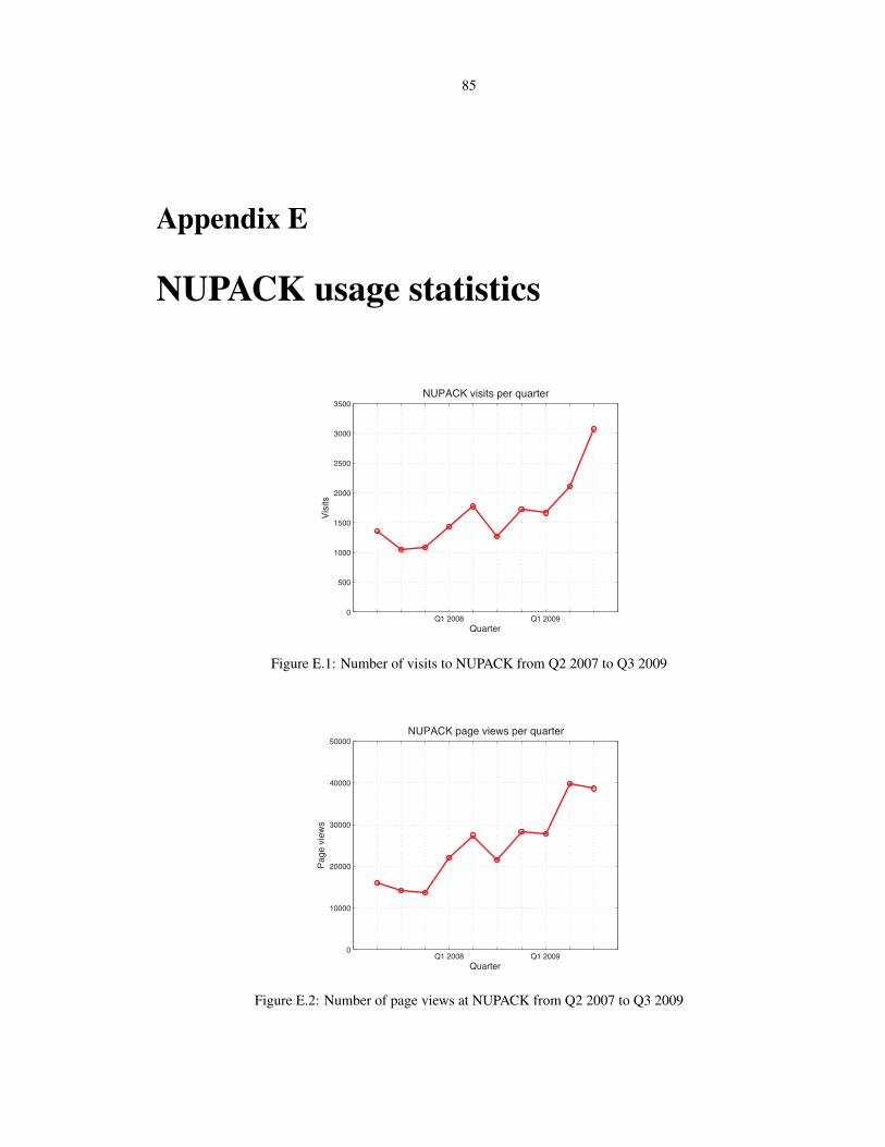
85
Appendix E
NUPACK usage statistics
Q1 2008 Q1 2009 0
500
1000
1500
2000
2500
3000
3500
Visi
ts
Quarter
NUPACK visits per quarter
Figure E.1: Number of visits to NUPACK from Q2 2007 to Q3 2009
Q1 2008 Q1 2009 0
10000
20000
30000
40000
50000
Page
vie
ws
Quarter
NUPACK page views per quarter
Figure E.2: Number of page views at NUPACK from Q2 2007 to Q3 2009


